Nonlinear Optimization: Introduction

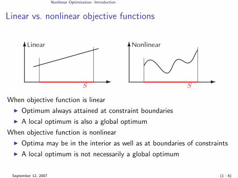
Linear vs. nonlinear objective functions

S

Linear

S

Nonlinear

When objective function is linear

I Optimum always attained at constraint boundaries

I A local optimum is also a global optimum

When objective function is nonlinear

I Optima may be in the interior as well as at boundaries of constraints

I A local optimum is not necessarily a global optimum

September 12, 2007 (1 : 6)

Nonlinear Optimization: Introduction

Convexity and optimality

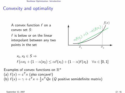
A convex function f on aconvex set S :

f is below or on the linearinterpolant between any twopoints in the set x

1x2

®f(x 1

) +(1 ¡®

)f(x 2)

f(x)

x1, x2 ∈ S ⇒f(αx1 + (1− α)x2

)≤ αf (x1) + (1− α)f (x2) ∀α ∈ [0, 1]

Examples of convex functions on Rn

(a) f (x) = cTx (also concave!)(b) f (x) = γ + cTx + 1

2xTQx (Q positive semidefinite matrix)

September 12, 2007 (2 : 6)

Nonlinear Optimization: Introduction

S ⊂ Rn

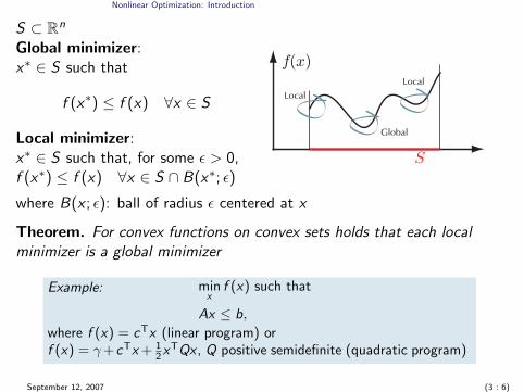
Global minimizer:x∗ ∈ S such that

f (x∗) ≤ f (x) ∀x ∈ S

Local minimizer:x∗ ∈ S such that, for some ε > 0,f (x∗) ≤ f (x) ∀x ∈ S ∩ B(x∗; ε)

S

Global

LocalLocal

f(x)

where B(x ; ε): ball of radius ε centered at x

Theorem. For convex functions on convex sets holds that each localminimizer is a global minimizer

Example: minx

f (x) such that

Ax ≤ b,

where f (x) = cTx (linear program) orf (x) = γ+cTx + 1

2xTQx , Q positive semidefinite (quadratic program)

September 12, 2007 (3 : 6)

Nonlinear Optimization: Introduction

Proof. Let x∗ be a local minimizer. Then ∃ε > 0 s. t.f (x∗) ≤ f (x) ∀x ∈ S ∩ B(x∗; ε).

Let x ∈ S arbitrarily. Will show f (x∗) ≤ f (x).

S convex ⇒ αx + (1− α)x∗ = xα ∈ S ∀α ∈ [0, 1]

Choose α > 0 such that xα ∈ S ∩ B(x∗; ε)

x∗ local min ⇒

f (x∗) ≤ f (xα) = f(αx + (1− α)x∗

)≤ [f convex]

≤ αf (x) + (1− α)f (x∗),

that is,

αf (x∗) ≤ αf (x) α > 0 ⇒f (x∗) ≤ f (x)

�

September 12, 2007 (4 : 6)

Nonlinear Optimization: Introduction

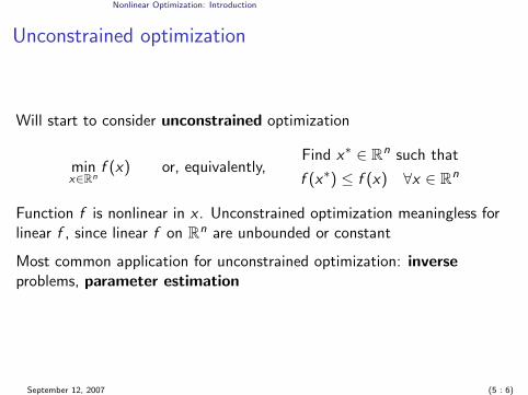
Unconstrained optimization

Will start to consider unconstrained optimization

minx∈Rn

f (x) or, equivalently,Find x∗ ∈ Rn such that

f (x∗) ≤ f (x) ∀x ∈ Rn

Function f is nonlinear in x . Unconstrained optimization meaningless forlinear f , since linear f on Rn are unbounded or constant

Most common application for unconstrained optimization: inverseproblems, parameter estimation

September 12, 2007 (5 : 6)

Nonlinear Optimization: Introduction

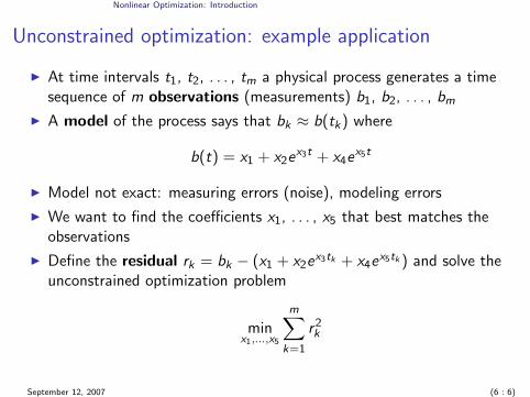
Unconstrained optimization: example application

I At time intervals t1, t2, . . . , tm a physical process generates a timesequence of m observations (measurements) b1, b2, . . . , bm

I A model of the process says that bk ≈ b(tk) where

b(t) = x1 + x2ex3t + x4e

x5t

I Model not exact: measuring errors (noise), modeling errors

I We want to find the coefficients x1, . . . , x5 that best matches theobservations

I Define the residual rk = bk − (x1 + x2ex3tk + x4e

x5tk ) and solve theunconstrained optimization problem

minx1,...,x5

m∑k=1

r2k

September 12, 2007 (6 : 6)