Nonlinear Analysis: Real World Applications 50 (2019) 342–364

Contents lists available at ScienceDirect

Nonlinear Analysis: Real World Applications

www.elsevier.com/locate/nonrwa

Vibrations of a Gao beam subjected to a moving mass

B. Dyniewicz a, C.I. Bajer a, K.L. Kuttler b, M. Shillor c,∗

a Institute of Fundamental Technological Research, Polish Academy of Sciences, Pawińskiego5b, 02-106 Warszawa, Polandb Retiredc Department of Mathematics and Statistics, Oakland University, Rochester, MI 48309, USA

a r t i c l e i n f o

Article history:Received 14 December 2018Received in revised form 14 May 2019Accepted 15 May 2019Available online xxxx

Keywords:Dynamic vibrationsBuckling of a Gao beamMoving point-load

a b s t r a c t

This paper models, analyzes and simulates the vibrations of a nonlinear Gao beamthat is subjected to a moving mass or a massless point-force. Such problems arisenaturally in transportation systems such as trains or trams. The dynamics of thesystem as the mass or the force move on the beam are investigated numericallyin the cases when the vibrations are about a buckled state, and in the cases whenthe mass is positive or vanishes. The simulations are compared to those of theEuler–Bernoulli linear beam and the differences are highlighted. It is seen that thelinear beam may be used only when the loads are small, while the Gao beam allowsfor moderate loads. The simulations are based on a time-marching finite elementsalgorithm for the model that has been developed and implemented. The results ofrepresentative and interesting computer simulations are depicted. The existence ofweak solutions of the model is established using a variational formulation of theproblem and results about variational set-inclusions.©2019 The Authors. Published by Elsevier Ltd. This is an open access article under the

CC BY-NC-ND license (http://creativecommons.org/licenses/by-nc-nd/4.0/).

1. Introduction

The motion of a point load on a metallic beam is of considerable importance in many applications,especially in railway systems, but also in construction (e.g., cranes) and many others. This explains therich and extensive scientific literature on the subject, see, e.g., [1,2] or [3]. Their fundamental importance inrailway transportation lies in the fact that the dynamic vibrations of the rail systems, when trains or tramstravel them, may cause unwanted damage to the supports and cause unwanted noise [4] and dynamic wear.Indeed, there is a need for accurate prediction of such vibrations and their effects on the reliability of thesystem it is important to understand and possibly control the noise generated by such processes.

This work is a contribution to the field and deals with accurate predictions of the system vibrations. It isa continuation of the study of the dynamic of systems that include the so-called ‘Gao beam,’ the equation

∗ Corresponding author.E-mail addresses: bdynie@ippt.gov.pl (B. Dyniewicz), cbajer@ippt.gov.pl (C.I. Bajer), klkuttler@gmath.com

(K.L. Kuttler), shillor@oakland.edu (M. Shillor).

https://doi.org/10.1016/j.nonrwa.2019.05.0071468-1218/© 2019 The Authors. Published by Elsevier Ltd. This is an open access article under the CC BY-NC-ND license(http://creativecommons.org/licenses/by-nc-nd/4.0/).

B. Dyniewicz, C.I. Bajer, K.L. Kuttler et al. / Nonlinear Analysis: Real World Applications 50 (2019) 342–364 343

of motion of which allows for vibrations about buckled states, [5–7]. We model, analyze and investigatecomputationally the horizontal motion of a vertical point-load that has either mass (inertial) or is massless,on a metallic rail and the resulting oscillations of the system. Our study is motivated, in part, by the previousworks on railway systems, see, e.g., [8,9] and the references therein. This subject has been extensively treatedin many publications, however, the assumptions and mechanical models used by various researchers wereincomplete and sometimes too simplistic. First, the track was subjected to a set of massless forces appliedwith more or less complex oscillators. Moreover, the dynamic properties and responses were not affected bythe additional inertia of the wheel-sets, which are invariably present in transportation applications. Indeed,their mass is about 750 kg per wheel and, hence, cannot be neglected, see e.g., [10,11]. Second, the axialforces in the rails were too simplistic. Third, the temperature variations in the rails can be more than 40 Cduring a day and more than 70 C during a year. Such variations in the temperature cause significant changesin the stresses in the system and the mathematical models for the structures must take these processes intoaccount. This work addresses the first and second issues, while the inclusion of thermal effects will be studiedin the future.

Models for a Gao beam were derived and simulated in [5,12–14] (see also the references therein). Theywere investigated mathematically and computationally in [6,7,15–19]. Basic mathematical analysis of themodel can be found in [6] where the solutions existence was established and problems that involve contactstudied. The dynamic contact of a Gao beam with a reactive or rigid foundation was described in [19]. Thecase of vibrations of a Gao beam whose end is restricted to move between two rigid or reactive stops wasstudied in [15], and the analysis of the problem of two coupled Gao beams connected via a joint with a gapcan be found in [18]. Vibration characteristic of contacting one-dimensional structures with a Gao beam wereconducted in [17], where the model, existence of weak solutions, and computer simulations can be found.Finally, an interesting problem was studied in [7] where the growth of a crack in a Gao beam was analyzedand simulated. Concerning models for contact, we refer to [20] and the many references therein.

The model we construct for the dynamics of a force that acts on a point-mass or massless that is movingon a straight rail, assumed to be of the Gao type, results in an unusual coupled system of a nonlinear beamequation and an ordinary differential equation for the motion of the mass. The system is given in (2.1) and(2.6). For the sake of generality, we assume that the horizontal motion of the point-mass and the load actingon it are time dependent, possibly periodic. We use our basic result in [21] to prove that the system, whichhas an unusual form, has a weak solution.

Next, we develop a 2D space–time FEM numerical algorithm for the model. However, in the simulations,for the sake of simplicity, we assume that the point-mass is moving with a constant velocity and the load onit is constant. Even this slightly simpler setting still contains most of the interest in the problem. Allowingfor periodic oscillations of the mass and variable loads are of interest, and will be studied in the sequel. In thesimulations algorithm, the FEM method allows us to derive characteristic matrices that deal well with thenonlinear terms in the differential equation. The numerical examples show the efficiency of the computationalmethod. In particular, they clearly exhibit the difference between the classical linear Euler–Bernoulli beamand the Gao beam model. The nonlinear terms significantly change the dynamic response and affect theinterplay between the stiffness of the beam and the frequency of the vibrations. The computer simulationsstudy the influence of the compressive force on the dynamic response of the Gao beam to a massless orinertial load. The system’s sensitivity to the horizontal traction force, load component and to its velocityare presented. Moreover, we use repeating crossing of the load over the whole span of the beam to exhibitthe difference in displacements as a function of time. We also investigate the advantages of the Gao modelas compared with the commonly used Euler–Bernoulli model.

We now describe the remaining sections of this paper. The ‘classical formulation’ of the model is presentedin Section 2. We choose the material constitutive law to be viscoelastic of the Gao type. To model the movingpoint-mass we use the Dirac distribution and the associated Renaudot condition. This leads to a coupled

344 B. Dyniewicz, C.I. Bajer, K.L. Kuttler et al. / Nonlinear Analysis: Real World Applications 50 (2019) 342–364

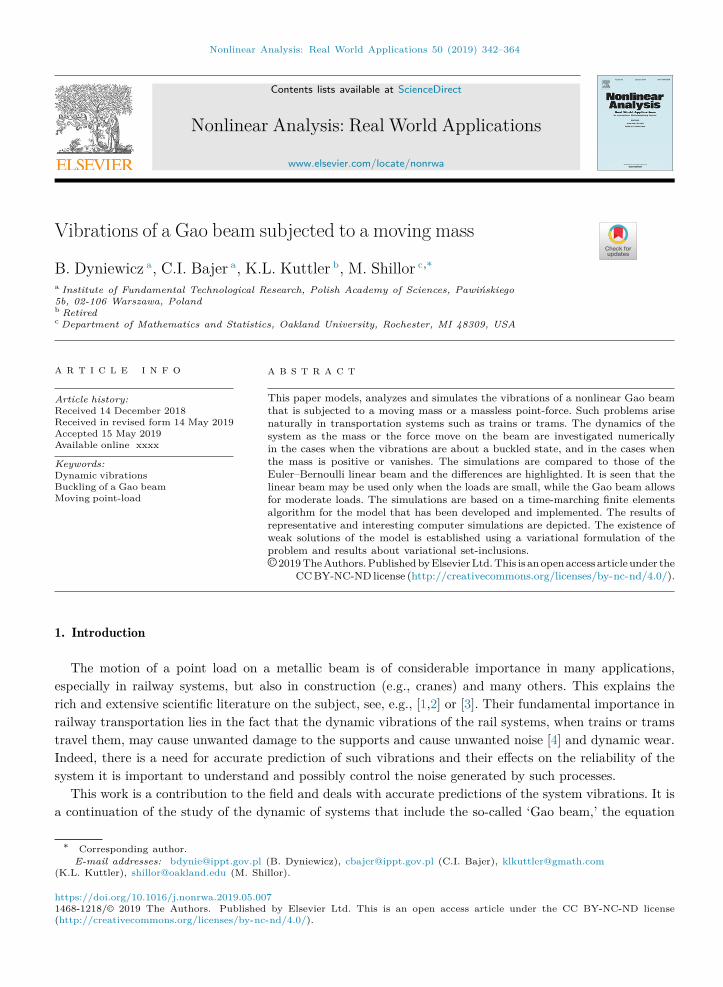
Fig. 1. The Gao beam without a moving load; w(x, t) denotes the displacement of the central axis. The lengths are scaled so thatL = 1.

system that consists of the dynamic Gao beam equation with the point-mass added, and the Renaudotcondition at the position of the mass. For the sake of generality, we allow the force that acts on the massand the velocity of the mass to be time-dependent. The existence of a weak or variational solution to themodel is presented in Section 3, based on an interesting version of a theorem in [21]. A numerical space–timeFEM scheme for the problem is constructed in Section 4. The convergence of the algorithm remains an openquestion. Moreover, as was noted above, we assume in the simulations that the point-load and the velocityof the mass are time-independent, and the beam is elastic. The implementation of the algorithm and sixnumerical simulations of the problem are depicted in Section 5. The paper concludes in Section 6 with someopen questions.

2. The model

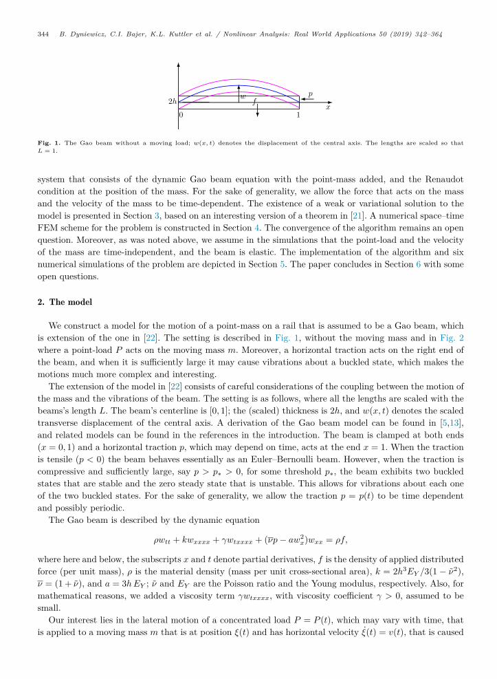
We construct a model for the motion of a point-mass on a rail that is assumed to be a Gao beam, whichis extension of the one in [22]. The setting is described in Fig. 1, without the moving mass and in Fig. 2where a point-load P acts on the moving mass m. Moreover, a horizontal traction acts on the right end ofthe beam, and when it is sufficiently large it may cause vibrations about a buckled state, which makes themotions much more complex and interesting.

The extension of the model in [22] consists of careful considerations of the coupling between the motion ofthe mass and the vibrations of the beam. The setting is as follows, where all the lengths are scaled with thebeams’s length L. The beam’s centerline is [0, 1]; the (scaled) thickness is 2h, and w(x, t) denotes the scaledtransverse displacement of the central axis. A derivation of the Gao beam model can be found in [5,13],and related models can be found in the references in the introduction. The beam is clamped at both ends(x = 0, 1) and a horizontal traction p, which may depend on time, acts at the end x = 1. When the tractionis tensile (p < 0) the beam behaves essentially as an Euler–Bernoulli beam. However, when the traction iscompressive and sufficiently large, say p > p∗ > 0, for some threshold p∗, the beam exhibits two buckledstates that are stable and the zero steady state that is unstable. This allows for vibrations about each oneof the two buckled states. For the sake of generality, we allow the traction p = p(t) to be time dependentand possibly periodic.

The Gao beam is described by the dynamic equation

ρwtt + kwxxxx + γwtxxxx + (νp− aw2x)wxx = ρf,

where here and below, the subscripts x and t denote partial derivatives, f is the density of applied distributedforce (per unit mass), ρ is the material density (mass per unit cross-sectional area), k = 2h3EY /3(1 − ν2),ν = (1 + ν), and a = 3hEY ; ν and EY are the Poisson ratio and the Young modulus, respectively. Also, formathematical reasons, we added a viscosity term γwtxxxx, with viscosity coefficient γ > 0, assumed to besmall.

Our interest lies in the lateral motion of a concentrated load P = P (t), which may vary with time, thatis applied to a moving mass m that is at position ξ(t) and has horizontal velocity ξ(t) = v(t), that is caused

B. Dyniewicz, C.I. Bajer, K.L. Kuttler et al. / Nonlinear Analysis: Real World Applications 50 (2019) 342–364 345

Fig. 2. The Gao beam with a moving load P (t) that acts on m at x = ξ(t).

by a horizontal applied force f∗(t). Here and below, a dot above a symbol represents the time derivative.Moreover, unlike our previous work [22], here the traction at x = 1 does not vanish, p > 0, and is largeenough to cause buckling.

To obtain the modifications of the model caused by the moving mass, which leads to non-constant density,we use Newton’s law of motion in its general form, i.e.,

ddt (MV ) = F,

where F is the total force, M is a variable mass and V is its velocity, so that MV is the system momentum.A careful examination of the forces and the rate of change of the momentum shows that the term ρwtt

has to be replaced byρwtt +mδ(x− ξ(t))wtt +mδ′(x− ξ(t))v(t)wt.

Here, δ(x) is the Dirac function (actually a distribution centered at the origin) and δ′(x) is its distributionalderivative. Next, we represent the load on the mass by δ(x − ξ(t))P (t). Finally, the equation of horizontalmotion of the mass, in absence of friction, is just

mξ = f∗.

The ‘classical formulation’ of the dynamic model for a viscoelastic beam with finite deformations and amoving point-load is as follows.

Problem 2.1. Given the external force f = f(x, t), the horizontal force f∗(t), the traction p = p(t), andthe point load P = P (t); find the displacement field w = w(x, t), for x ∈ (0, 1) and the position of the massξ(t), t ∈ [0, T ], such that

ρwtt +mδ(x− ξ)wtt(ξ, t) +mδ′(x− ξ(t))v(t)wt + kwxxxx + γwtxxxx

−(aw2x − νp)wxx = ρf + δ(x− ξ)P, (2.1)mξ = f∗, (2.2)

w(0, t) = wx(0, t) = 0, (2.3)w(L, t) = wx(L, t) = 0, (2.4)

w(x, 0) = w0(x), wt(x, 0) = v0(x), ξ(0) = ξ0, v(0) = ξ00. (2.5)

The initial data w0(x), v0(t), ξ0 and ξ00 are given and have the appropriate smoothness. We note herethat

ξ(t) = ξ0 +∫ t

0ξ(τ) dτ.

This, in particular, implies that the model ceases to make sense beyond the time T ∗ when either ξ(T ∗) = 0or ξ(T ∗) = 1, when the load completes a transit over the beam. Thus, below, T is assumed to satisfy T ≤ T ∗.

346 B. Dyniewicz, C.I. Bajer, K.L. Kuttler et al. / Nonlinear Analysis: Real World Applications 50 (2019) 342–364

The vertical acceleration of the mass particle is given by the Renaudot formula [10], which is the totaltime derivative of w(ξ, t),

d2w(ξ, t)dt2 =

[wtt + 2ξwxt + ξwx + ξ2wxx

]x=ξ(t) . (2.6)

The derivatives on the right-hand side are evaluated at the position of the mass ξ(t). The horizontalacceleration is v(t) = ξ = f∗/m.

Remark 2.2. We note here that there is an inaccuracy in formula (2.6) in [22], and the correct expressionis (2.6). However, the mistake there did not affect the results since, all that was used was formula (2.7) there(when v = const.), which is exactly the same as (2.7) here.

When v = ξ is constant, then ξ(t) = vt, ξ = 0 and (2.6) reads

d2w(vt, t)dt2 =

[wtt + 2vwxt + v2wxx

]x=vt

. (2.7)

Remark 2.3. In later stages of this work we plan to take into account friction into the horizontal motion ofthe mass. This may be done by using a beam-rod system. This, however, introduces considerable additionalcomplexity which is not warranted at this stage.

The system is nonlinear and of unusual form and so it is natural to consider a weak or variationalformulation, especially since the Dirac ‘delta function’, and its derivative, which are distributions, appear in(2.1), and so we expect the velocity wt to be discontinuous at x = ξ(t).

3. Existence

In this section we construct a variational formulation of the model, provide the assumptions on the inputdata, then state the existence result and provide its proof. First, we rewrite the system,

ρwtt + ddt (mδ(x− ξ)wt(ξ, t)) + kwxxxx + γwtxxxx

−(aw2x − νp)wxx = ρf + δ(x− ξ)P, (3.1)

mξ = f∗, (3.2)w(0, t) = wx(0, t) = 0, (3.3)w(1, t) = wx(1, t) = 0, (3.4)w(x, 0) = w0(x), wt(x, 0) = v0(x). (3.5)

Next, we derive a variational formulation for the model. Let V be the Hilbert space

V =u ∈ H2 (0, 1) : u (0) = ux (0) = u (1) = ux (1) = 0

,

and letH = L2 (0, 1) , W = closure of V in H1 (0, 1) .

These spaces contain the boundary conditions, since the beam is clamped at both ends. The problem isformulated in terms of mappings from V to its dual space V ′, where

V ≡ L2 (0, T ;V ) , W ≡ L2 (0, T ;W ) .

B. Dyniewicz, C.I. Bajer, K.L. Kuttler et al. / Nonlinear Analysis: Real World Applications 50 (2019) 342–364 347

We begin with the inertial term and let ψ (x) ∈ V and ϕ (t) ∈ C∞c (0, T ) and use ψ(x)ϕ(t) as a test

function. We multiply the equation and integrate over space and time, thus,∫ 1

0

∫ T

0

ddt (mδ(x− ξ)wt(ξ, t))ϕ (t)ψ (x) dtdx

=∫ 1

0

([(mδ(x− ξ)wt(ξ, t))ϕ (t)ψ (x) |T0

−∫ T

0(mδ(x− ξ)wt(ξ, t))ϕ′ (t)ψ (x)] dt) dx

= −∫ T

0

∫ 1

0(mδ(x− ξ)wt(ξ, t))ϕ′ (t)ψ (x) dxdt

= −∫ T

0mwt (ξ, t)ϕ′ (t)ψ (ξ) dt. (3.6)

Here, we used the boundary conditions and the fact that ϕ vanishes at t = 0, T . Next, we define the operatorB (t) : V → V ′ as

⟨B (t)u, y⟩ = mu (ξ (t)) y (ξ (t)) .

It follows that B (t) is symmetric and bounded because pointwise evaluation is continuous on V . Next, theusual arguments from calculus yield

⟨B′ (t)u, y⟩ = (mux (ξ (t)) y (ξ (t)) +mu (ξ (t)) yx (ξ (t))) ξ (t) . (3.7)

We assume that f∗ is continuous and bounded, hence it follows from (3.2) that ξ is bounded and continuous.Therefore, continuity of pointwise evaluation on H1 (0, L) guarantees that there exists a constant C,dependent on m and the bound for ξ, such that

⟨B′ (t)u, y⟩ ≥ −C (∥u∥V ∥y∥W + ∥u∥W ∥y∥V ) . (3.8)

Furthermore, we let ε > 0 be given, then we have the inequality

∥z∥H1 ≤ ε ∥z∥V + Cε |z|H

Applying it to (3.8) and adjusting the constants, we obtain,

⟨B′ (t)u, u⟩ ≥ −C (||u||V (ε ∥u∥V + Cε |u|H))≥ −ε ||u||2V − Cε |u|2H . (3.9)

While Cε may be quite large ε can be made as small as desired. Also, (3.7) shows that B′ is continuous asa map from V to V ′.

For the sake of simplicity, we assume that the density ρ = 1, although the method below may be appliedto a density that is inhomogeneous and possibly time dependent, ρ = ρ(x, t). Using the boundary conditions,we find ∫ T

0

∫ 1

0(kwxxxx + γwtxxxx)ψ (t)ϕ (x) dxdt

=∫ T

0

∫ 1

0(kwxx + γwtxx)ψ (t)ϕxx (x) dxdt.

Let L : V → V ′ be the operator

⟨Lu,w⟩ = ⟨Lu,w⟩V ′,V ≡∫ 1

0uxxwxxdx.

348 B. Dyniewicz, C.I. Bajer, K.L. Kuttler et al. / Nonlinear Analysis: Real World Applications 50 (2019) 342–364

Now, we consider the nonlinear term, and define N : V → V ′ by

⟨Nw, u⟩ ≡ −∫ 1

0(aw2

x − νp)wxxudx.

We also need an approximate operator which comes from truncating. To that end, let

Qr (x) ≡x2 if |x| < r,r2 if |x| ≥ r.

Next, we consider the truncated operator

⟨Nrw, u⟩ ≡ −∫ 1

0(aQr (wx) − νp)wxxudx.

Let Φ′r (x) = Qr (x) ,Φr (0) = 0. Then, using the boundary conditions we obtain

⟨Nrw,w⟩ = −∫ 1

0(aQr (wx) − νp)wxxwdx

= −∫ 1

0(aΦ′

r (wx)wxxw − νpwxxw) dx

= −∫ 1

0ad

dx (Φr (wx))w dx+∫ 1

0νpwxxwdx

=∫ 1

0aΦr (wx)wx dx+

∫ 1

0νpwxxw dx.

Note that the first term is nonnegative. Below we derive an estimate for w in V that is independent of r andthen by choosing r large enough we obtain a solution to the non-truncated problem. But first, we consider∥Nrw −Nrw∥V ′ .

|⟨Nrw −Nrw, v⟩| ≤∫ 1

0νp (wxx − wxx) vdx

+ |a|∫ 1

0|Φr (wx) − Φr (wx)| |vx| dx

=∫ 1

0νp (wx − wx) vxdx

+ |a|∫ 1

0|Φr (wx) − Φr (wx)| |vx| dx

≤∫ 1

0νp (wx − wx) vxdx

+ |a|Kr

∫ 1

0|wx − wx| |vx| dx

≤ Cr ∥w − w∥W ∥v∥W .

Here, Kr = 2r is the Lipschitz constant of Φr, and Cr is a positive constant that depends on r. Thus, sinceV is dense in W ,

∥Nrw −Nrw∥V ′ ≤ Cr ∥w − w∥W . (3.10)

To simplify slightly the presentation, we let w (t) = w0 +∫ t

0 u (s) ds and write the problem in terms of thebeams velocity u.

We first consider the problem in which N is replaced with Nr. Our abstract formulation of the truncatedproblem becomes

((I +B (t))u)′ + kLw + γLu+Nrw = f + δ (· − ξ)P, (3.11)

w (t) = w0 +∫ t

0u (s) ds, (3.12)

u (0) = v0, (3.13)

where⟨δ (· − ξ)P, u⟩ ≡

∫ T

0P (t)u (t, ξ (t)) dt. (3.14)

B. Dyniewicz, C.I. Bajer, K.L. Kuttler et al. / Nonlinear Analysis: Real World Applications 50 (2019) 342–364 349

We now assume that w ∈ C ([0, T ] ;V ) is given. Then, it follows from the usual considerations (see,e.g., [21,23–25] and the many references therein) that there exists a solution u to (3.11)–(3.13) such thatu ∈ V, u′ ∈ V ′. However, we do not know if (3.12) holds. It follows from (3.9) that

γ ⟨Lu, u⟩ + 12

∫ T

0⟨(I +B′)u, u⟩ dt ≥ δ (ω)

∫ T

0∥u∥2

V ds− C |u|2H ,

which is sufficient to allow us to use the main result of [21] along with an exponential shift argument. Then,the monotonicity of L and the estimates for B′ show that the solution u is unique. Next, assume that w andw are given and let (w, u) and (w, u) be the corresponding solutions, hence,

((I +B (t))u)′ + kLw + γL (u) +Nrw = f + δ (· − ξ)P,((I +B (t)) u)′ + kLw + γL (u) +Nrw = f + δ (· − ξ)P.

Then, we let((I +B (t)) (u− u))′ + kL (w − w) + γL (u− u) +Nrw −Nrw = 0

act on u− u and use the integration by parts theorems developed in [21] to obtain, for B (t) ≡ I+B (t), theinequality

12

⟨B (u− u) , u− u

⟩(t) + 1

2

∫ t

0⟨B′ (u− u) , u− u⟩ ds

+ k ||w (t) − w (t)||2V + γ

∫ t

0||u− u||2V ds ≤ Cr ||w (t) − w (t)||2.

W

It follows from the compactness of the embedding of V into W that

12 |u− u|2H (t) +

∫ t

0⟨B′ (u− u) , u− u⟩ ds+ k ||w (t) − w (t)||2V + γ

∫ t

0||u− u||2V ds

≤ ε ∥w (t) − w (t)∥2V + Cε.r |w (t) − w (t)|2H .

Now, we use the estimates in (3.9) for B′ and obtain

12 |u− u|2H (t) −

∫ t

0ε ∥u− u∥2

V ds− Cε

∫ t

0|u− u|2H ds+ k ||w (t) − w (t)||2V

+γ∫ t

0||u− u||2V ds ≤ ε ∥w (t) − w (t)∥2

V + Cε.r |w (t) − w (t)|2H , (3.15)

where ε can be chosen as small as desired.We wish to use a fixed point argument. To that end for a given w let u be the solution of (3.11)–(3.13)

that corresponds to w and we let

Fw (t) ≡ w0 +∫ t

0u (s) ds.

It follows from the estimates above that,

|Fw (t) − Fw (t)|H ≤∫ t

0|u (s) − u (s)| ds.

Choosing ε sufficiently small in (3.15), we find that there is a constant Ck,γ,r > 0, depending on k, r, γ suchthat

|u− u|H (t) ≤ Ck,γ,r |w − w|H (t) ,

and so, there is another constant C that depends on k, γ, r such that

|Fw (t) − Fw (t)|H ≤ C

∫ t

0|w − w|H (s) ds.

350 B. Dyniewicz, C.I. Bajer, K.L. Kuttler et al. / Nonlinear Analysis: Real World Applications 50 (2019) 342–364

It follows from iteration of the inequality that a high enough power of F is a contraction map on C ([0, T ] ;H)and so there exists a unique fixed point w of F , hence

w (t) = Fw (t) = w0 +∫ t

0u (s) ds,

which is the unique solution of (3.11)–(3.13). This has proved the following theorem.

Theorem 3.1. For each r > 0 there exists a unique solution w to the approximate problem (3.11)–(3.13)and it satisfies w ∈ V and ((I +B (·))w)′ ∈ V ′.

Actually, when r is sufficiently large, this estimate shows the existence of a unique solution for the originalproblem without the truncation. To see this, it suffices to obtain an estimate on wx that is independent ofr. To that end, we let (3.11) act on u. Then, using the estimate for B′ in (3.9), we obtain

12 |u (t)|2H − ε

∫ t

0||u (s)||2V ds− Cε

∫ t

0|u (s)|2H ds+ k ||w (t)||2V − k ||w0||2 + γ

∫ t

0||u||2V ds

−∫ t

0

∫ 1

0(aQr (wx) − νp)wxxudxds ≤ Cε + ε

∫ t

0||u (s)||2V ds, (3.16)

where Cε depends on f and P . We now consider the nonlinear term and using the boundary conditions, wefind

−∫ t

0

∫ 1

0(aQr (wx) − νp)wxxudxds = −

∫ t

0

∫ 1

0aΦr (wx)x udxds+

∫ t

0

∫ 1

0νpwxxudxds

≥∫ t

0

∫ 1

0aΦr (wx)uxdxds− C

(∫ t

0||w||2V ds+

∫ t

0|u|2H ds

).

Letting Ψr (x) =∫ x

0 Φr (y) dy, it follows that Ψr (x) ≥ 0 and then,

=∫ 1

0aΨr (wx) dx−

∫ 1

0aΨr (w0x) dx−

(∫ t

0ε ||w||2V ds+ Cε

∫ t

0|u|2H ds

)≥ −

∫ 1

0aΨr (w0x) dx−

(∫ t

0ε ||w||2V ds+ Cε

∫ t

0|u|2H ds

)≥ −C − C

(∫ t

0||w||2V ds+

∫ t

0|u|2H ds

),

for a constant C that is independent of r, for all r sufficiently large. Here, we used the fact that w0x isbounded since w0 ∈ V . Thus, (3.16) implies

12 |u (t)|2H − ε

∫ t

0||u (s)||2V ds− Cε

∫ t

0|u (s)|2H ds+ k ||w (t)||2V − k ||w0||2V + γ

∫ t

0||u||2V ds

−(C + C

(∫ t

0||w||2V ds+

∫ t

0|u|2H ds

))≤ Cε + ε

∫ t

0||u (s)||2V ds.

Choosing ε small enough, depending on γ, we obtain

|u (t)|2H + γ

2

∫ t

0||u||2V ds+ k ||w (t)||2V ≤ Cε + k ||w0||2V + C

∫ t

0||w||2 ds+

∫ t

0|u|2H ds.

Then, Gronwall’s inequality establishes a bound for ||w (t)||V that is independent of r. This yields thefollowing corollary, which is the main theoretical result in this work.

B. Dyniewicz, C.I. Bajer, K.L. Kuttler et al. / Nonlinear Analysis: Real World Applications 50 (2019) 342–364 351

Theorem 3.2. There exists a unique solution u to the problem

((I +B (t))u)′ + kLw + γLu+Nw = f + δ (· − ξ)P, (3.17)

w (t) = w0 +∫ t

0u (s) ds, (3.18)

u (0) = v0, (3.19)

u ∈ V and ((I +B (·))u)′ ∈ V ′. Moreover, when r is chosen large enough this is the unique weak solution ofthe original problem, (3.1)–(3.5), without the truncation.

We conclude that there exists a unique weak solution of the model. We note that although γ > 0, it maybe as small as we wish, however, the limit γ → 0 cannot be obtained from these considerations.

4. Numerical algorithm

We develop a numerical scheme for the model, and the results of its implementation are presented in thefollowing section.

There are numerous methods to obtain numerical approximations for initial–boundary problems. In someproblems, and ours is of such a type, the standard methods either fail or cannot be directly applied to thedifferential equations. In this problem the governing equation is nonlinear and has varying coefficients. In theclassical finite element method, FEM, such problems are simplified and the nonlinear terms are linearized,which may cause the results to diverge from the exact ones. In our model, this occurs when the inertialpoint crosses the element’s boundary or passes to a successive time layer in the process of time integrationof the equation of motion. Such a traveling point carries the momentum perpendicular to the beam’s axis,along the beam. In such a case, the numerical algorithms based on routine approach of FEM do not providecorrect results.

To address this problem, we used the space–time finite element approach. Continuous approximationswere applied to both the spatial and temporal variables at the same time [26–28]. This allows for a weakformulation of the problem that cannot be simply formulated while separating time from space. There existbroad literature devoted to space–time finite element method, STFEM, for various problems, see, e.g., [29–31]and the references therein.

The main difference between the classical FEM and the STFEM lies in the interpolation functions:

q(x, t) = N(x) · T(t) qe (FEM), q(x, t) = N(x, t) qe (STFEM).

In FEM the interpolation in space N(x) and time T(t) are done separately while in STFEM the interpolationis carried on jointly N(x, t). Thus, FEM can be considered as a particular case of STFEM.

We discretize the equation of motion (2.1) using space–time rectangular finite elements, depicted in Fig. 3,where the element subdomain is

Ωbh = (x, t) : 0 ≤ x ≤ b, 0 ≤ t ≤ h.

Here, h = t is the time step, so that if T is the final time, we have nT = T/h time steps and nS = 1/bspacial elements (recall that L = 1).

We take into account the pure bending process described by the 4th order x-derivative (see, (2.1)). Inthis beam model, the influence of the shear forces on the potential energy, and therefore on the deflection,are neglected. Then, the angle of rotation of the cross section is directly joined with the deflected neutralaxis of the beam. We use both deflections and rotations at nodal points of each element. Thus, there are

352 B. Dyniewicz, C.I. Bajer, K.L. Kuttler et al. / Nonlinear Analysis: Real World Applications 50 (2019) 342–364

Fig. 3. A space–time finite element domain Ωbh.

four degrees of freedom at each time layer of the element that allow to determine a third order polynomialin space. We use a velocity variant of the space–time discretization, therefore, the velocity in the beam finiteelement is represented by the nodal velocity parameters in two successive time steps. We denote the currentstate, which just has been obtained, by vt and the unknown state at the next time step by vt+h. Thus, wehave

v(x, t) =(

1 − t

h

)Nvt + t

hNvt+h , (4.1)

where [vt

vt+h

]=

[v1 ψ1 v2 ψ2 v3 ψ3 v4 ψ4

]T, (4.2)

is the nodal velocity vector and the shape functions N are given by

N = [N1, N2, N3, N4] , (4.3)

are chosen asN1 = 1 − 3x

2

b2 + 2x3

b3 , N2 = x− 2x2

b+ x3

b2 ,

N3 = 3x2

b2 − 2x3

b3 , N4 = −x2

b+ x3

b2 .

We see that the velocity vector v in (4.1) is interpolated from eight nodal values: four that are known froma previous time t and four unknown at time t + h. Now, we use (4.1) to calculate the displacements in theelement,

w(x, t) = w0(x) +∫ t

0v(x, t)dt

= Nwt +(t− t2

2h

)Nvt + t2

2hNvt+h, (4.4)

where the nodal displacement vector wt is known and composed of the deflections w and rotations ψ given attwo nodes of the space–time element at time t. The differential equation (2.1) allows us to write the virtualwork in the finite element as follows

Π =∫Ω

v∗ ρwtt + kwxxxx − aw2

xwxx + νpwxx

+ δ(x− vt)mwtt(vt, t) − δ(x− vt)P dxdt, (4.5)

where the virtual velocity v∗ with the parameter α is given by

v∗(x, t) = δ(t− αh) (Nv∗)T.

B. Dyniewicz, C.I. Bajer, K.L. Kuttler et al. / Nonlinear Analysis: Real World Applications 50 (2019) 342–364 353

We use this form, chosen from the various possible functions of virtual velocity distributions, because ofthe simplicity of the time integration of the energy functional Π and simple stability control. Here, α ∈ [0, 1]is a parameter that defines the equilibrium point in the time layer (similarly to β in the Newmark timeintegration scheme). It affects the accuracy and stability of the resulting time integrating scheme (for detailssee [32]). Integrating, formally, by parts the virtual work expression (4.5) leads to the following expression

Π =k∫Ω

v∗xxwxx dxdt+

∫Ω

v∗ ρvt − aw2

xwxx + νpwxx

+ δ(x− vt)m(vt + 2vvx + v2wxx)x=vt

− δ(x− vt)P

dxdt. (4.6)

To proceed with the numerical scheme, we need the following matrices: the element mass and stiffnesscharacteristic matrices are given by

M = ρ

⎡⎢⎢⎢⎢⎢⎢⎢⎢⎢⎢⎢⎢⎣

13b35

11b2

2109b70

−13b420

11b2

210b3

10513b2

420−b3

1409b70

13b2

42013b35

−11b2

210−13b2

420−b3

140−11b2

210b3

105

⎤⎥⎥⎥⎥⎥⎥⎥⎥⎥⎥⎥⎥⎦,

and

K = k

⎡⎢⎢⎢⎢⎢⎢⎢⎢⎢⎢⎢⎢⎣

12b3

6b2

−12b3

6b2

6b2

4b

−6b2

2b

−12b3

−6b2

12b3

−6b2

6b2

2b

−6b2

4b

⎤⎥⎥⎥⎥⎥⎥⎥⎥⎥⎥⎥⎥⎦+ νp

⎡⎢⎢⎢⎢⎢⎢⎢⎢⎢⎢⎢⎢⎣

65b

1110

−65b

110

110

2b15

−110

−b30

−65b

−110

65b

−1110

110

−b30

−110

2b15

⎤⎥⎥⎥⎥⎥⎥⎥⎥⎥⎥⎥⎥⎦.

To deal with the nonlinearity, we use a term in which the nonlinearity is frozen at the time t so that wt andvt are known,

Kn = a

∫ b

0NT [

Nxwt + (α− 0.5α2)hNxvt + 0.5α2hNxvt+h]2 Nxx dx. (4.7)

The explicit matrix form of Kn is provided in the Appendix.The general matrices representing the moving mass were derived by using linear shape functions as

described in [33],

Mm = m

⎡⎢⎢⎣(1 − κ)2 0 κ(1 − κ) 0

0 0 0 0κ(1 − κ) 0 κ2 0

0 0 0 0

⎤⎥⎥⎦ ,

Cm = 2mvb

⎡⎢⎢⎣κ− 1 0 1 − κ 0

0 0 0 0−κ 0 κ 00 0 0 0

⎤⎥⎥⎦ ,

etm = mv

bh

⎡⎢⎢⎣(1 − κ)(wi+1

2 − wi2 − wi+1

1 + wi1)

0κ(wi+1

2 − wi2 − wi+1

1 + wi1)

0

⎤⎥⎥⎦ .

354 B. Dyniewicz, C.I. Bajer, K.L. Kuttler et al. / Nonlinear Analysis: Real World Applications 50 (2019) 342–364

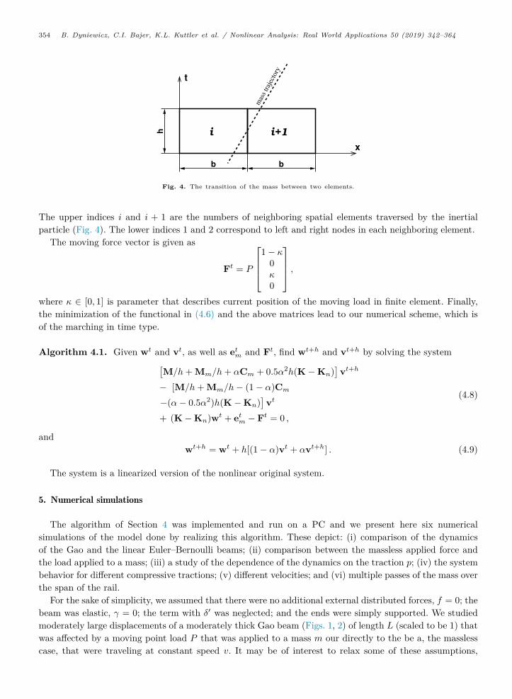
Fig. 4. The transition of the mass between two elements.

The upper indices i and i + 1 are the numbers of neighboring spatial elements traversed by the inertialparticle (Fig. 4). The lower indices 1 and 2 correspond to left and right nodes in each neighboring element.

The moving force vector is given as

Ft = P

⎡⎢⎢⎣1 − κ

0κ0

⎤⎥⎥⎦ ,where κ ∈ [0, 1] is parameter that describes current position of the moving load in finite element. Finally,the minimization of the functional in (4.6) and the above matrices lead to our numerical scheme, which isof the marching in time type.

Algorithm 4.1. Given wt and vt, as well as etm and Ft, find wt+h and vt+h by solving the system[

M/h+ Mm/h+ αCm + 0.5α2h(K − Kn)]

vt+h

− [M/h+ Mm/h− (1 − α)Cm

−(α− 0.5α2)h(K − Kn)]

vt

+ (K − Kn)wt + etm − Ft = 0 ,

(4.8)

andwt+h = wt + h[(1 − α)vt + αvt+h] . (4.9)

The system is a linearized version of the nonlinear original system.

5. Numerical simulations

The algorithm of Section 4 was implemented and run on a PC and we present here six numericalsimulations of the model done by realizing this algorithm. These depict: (i) comparison of the dynamicsof the Gao and the linear Euler–Bernoulli beams; (ii) comparison between the massless applied force andthe load applied to a mass; (iii) a study of the dependence of the dynamics on the traction p; (iv) the systembehavior for different compressive tractions; (v) different velocities; and (vi) multiple passes of the mass overthe span of the rail.

For the sake of simplicity, we assumed that there were no additional external distributed forces, f = 0; thebeam was elastic, γ = 0; the term with δ′ was neglected; and the ends were simply supported. We studiedmoderately large displacements of a moderately thick Gao beam (Figs. 1, 2) of length L (scaled to be 1) thatwas affected by a moving point load P that was applied to a mass m our directly to the be a, the masslesscase, that were traveling at constant speed v. It may be of interest to relax some of these assumptions,

B. Dyniewicz, C.I. Bajer, K.L. Kuttler et al. / Nonlinear Analysis: Real World Applications 50 (2019) 342–364 355

especially that v = const. The assumption that v = const. makes Eq. (2.2) unnecessary. We note that whilein [22] the traction at x = 1 was assumed to vanish and so there was no possibility for the beam to buckle,here we let p > 0 (compressive) and so the system may buckle when p > p∗, where p∗ is the critical value(see, e.g., [5–7]). We return to this point below and study this in more details.

The time integration of the algorithm for the data listed below was 10 µs. The beam was divided into 100finite elements with 202 degrees of freedom. The nonlinear terms were computed iteratively, hence each timestep took relatively longer time. The time it took for each simulation was about 48 s during 20,000 time stepsfor αv = 0.3 and p = 0.01, which was the time it took the load to travel the entire span. Most of computingtime was spent on recalculating the matrices related to the nonlinear effects. It was noticed, however, thatby increasing the time step and allowing for a larger error, the task could be performed in 10–20 s on a singleprocessor core. As was noted in [22, Section 4], to avoid the appearance numerical oscillations because ofthe nonlinear terms in the equations, we used an analytical evaluation of the coefficients, eliminating thisproblem.

The data set for a steel beam used in the simulations was:L = 100 [cm],β = 0.015,ν = 0.3, ρ = 7.7 β2L2

π = 5.5175 [g/cm]k = 0.57 β4L4

4π3 = 0.0233 [g cm3/µs2],a = 3.105 β2L2

π = 2.2249 [g cm/µs2],v = π

√k/ρ

L αv = 0.002 αv [cm/µs],m = 100ρL = 55175 [g]P = mg = 5.4071 ∗ 10−5 [g cm/µs2],p∗ = 0.71 [g cm/µs2],g = 9.8·10−10 [cm/µs2].

We used a nonstandard unit system [cm, g, µs] that allowed us to have all the values in the same range,which improved the conditioning of the system of algebraic equations and reduced the truncation errors.

We turn to describe the simulation results, which provide considerable insight into the system’s dynamics.The first set of computer experiments compares the vibrations of the Gao beam with those of the linearEuler–Bernoulli beam, when p = 0, so that the comparison is valid. The simulations exhibit the basicdifference in the dynamics of the two beam models and, as expected, the Gao beam behaves well for largeroscillations while the linear beam’s oscillations become unphysical, implying that the Euler–Bernoulli beammay be used only with small loads and small amplitudes. The comparison between the two beams, when theload is massless is depicted in Fig. 5, and when the load acts on a mass, in Fig. 6.

In the massless case, although the trajectories’ shapes have similar forms, the scales and the amplitudesof the vibrations are very different. Indeed, the amplitudes of the Euler–Bernoulli beam are very large andexceed any reasonable use of a linearized system. Thus, as was noted above, the linear model can be usefulonly when the loads are small. The Gao beam, on the other hand, behaves much better and the amplitudesare very reasonable. It exhibited stiffening with the amplitude and in the example the amplitudes were ten-fold smaller. We note that multiple passages of the point force without inertia have similar trajectories, bothat successive periods and in both beam models, but not equal in value. However, the lack of a mass leads tospurious oscillations created by the numerics that can clearly be seen. This comparison is very instructiveconcerning the applicability of the two models.

Different responses were exhibited in the case of the inertial load (m > 0), Fig. 6, were the differencesbetween the two models were even more pronounced. Whereas the Gao beam exhibited smooth regular os-cillations, the Euler–Bernoulli beam oscillated wildly with unreasonable form and amplitude. The advantageof using the Gao beam to obtain meaningful simulations was evident. Moreover, we notice that the inertia ofthe mass leads to the smoothing of the oscillations with good accuracy and no visible spurious oscillations. As

356 B. Dyniewicz, C.I. Bajer, K.L. Kuttler et al. / Nonlinear Analysis: Real World Applications 50 (2019) 342–364

Fig. 5. Comparison of the load trajectory and the vibrations of a linear Euler–Bernoulli and the Gao beam models, for m = 0 andp = 0. Notice the different vertical scales.

Fig. 6. Comparison of the load trajectory and the vibrations between a linear Euler–Bernoulli beam model and the Gao one, form > 0 and p = 0. Notice the different scales.

we discuss below, multiple passages of the point force without inertia produced similar shapes of trajectoriesat successive periods and in both beam models.

To gain deeper insight into the system dynamics, we compared the behavior of the Gao model when theload acted on a mass m (the inertial case), or acted directly on the beam, (the massless or non-inertial case),for six different values of the horizontal compressive traction p. In all the cases, we chose the values of thecompressive horizontal traction p to be above the critical value p∗ so that the beam exhibited buckling.

Numerical estimate of p∗, depicted in Fig. 7, showed it to be about p∗ = 0.71. Below this value thebeam vibrated about the zero equilibrium point, while above it about a buckled state. A study of thevibrations of the mid-point of the Gao beam, without the moving load, near the critical value p∗ in thecases p = 0.600, 0.708, 0.710 and 0.750 is depicted in Fig. 8. We note that there is no effective analytic wayto determine p∗.

The six numerical experiments are depicted in Fig. 9. It is clearly seen that the frequency of the oscillationsincreases with p. The difference between the inertial and massless cases was substantial and the heavymass changed the frequency considerably, although the amplitudes remained comparable. The importance

B. Dyniewicz, C.I. Bajer, K.L. Kuttler et al. / Nonlinear Analysis: Real World Applications 50 (2019) 342–364 357

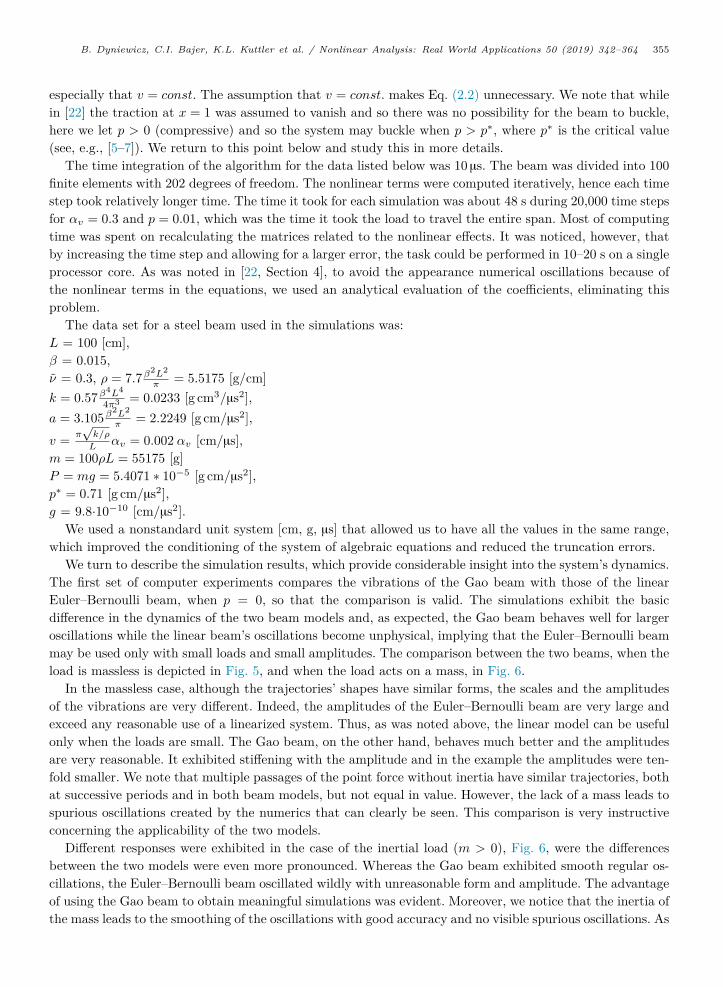
Fig. 7. The relative amplitude of the midpoint of the beam related to the amplitude of the initial deflection u0 for various values ofp. The value p∗ = 0.71 divides the buckled from the non-buckled states.

Fig. 8. The system oscillations at four values of p near the critical value p∗ = 0.71. The vibrations with p = 0.750 are about abuckled state.

of adding the mass in railway applications was mentioned in the introduction, and these results show itsimportance. We also note that the contact point of P or the mass, was above the neutral axis (i.e., w = 0),in the cases of p = 4.5 and p = 6.0, while for p was below p = 4.5 or p = 7.5 the contact point was beloww = 0. The behavior is well visible in Fig. 10, which depicts the deformed axes of the beam in time.

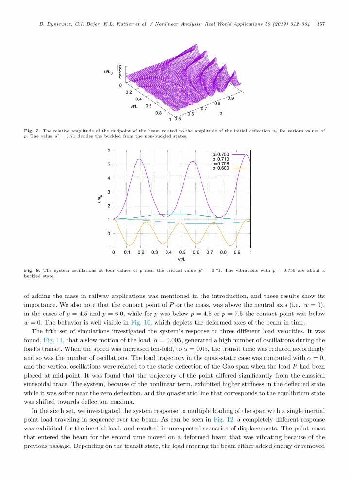
The fifth set of simulations investigated the system’s response to three different load velocities. It wasfound, Fig. 11, that a slow motion of the load, α = 0.005, generated a high number of oscillations during theload’s transit. When the speed was increased ten-fold, to α = 0.05, the transit time was reduced accordinglyand so was the number of oscillations. The load trajectory in the quasi-static case was computed with α = 0,and the vertical oscillations were related to the static deflection of the Gao span when the load P had beenplaced at mid-point. It was found that the trajectory of the point differed significantly from the classicalsinusoidal trace. The system, because of the nonlinear term, exhibited higher stiffness in the deflected statewhile it was softer near the zero deflection, and the quasistatic line that corresponds to the equilibrium statewas shifted towards deflection maxima.

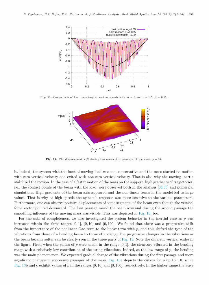
In the sixth set, we investigated the system response to multiple loading of the span with a single inertialpoint load traveling in sequence over the beam. As can be seen in Fig. 12, a completely different responsewas exhibited for the inertial load, and resulted in unexpected scenarios of displacements. The point massthat entered the beam for the second time moved on a deformed beam that was vibrating because of theprevious passage. Depending on the transit state, the load entering the beam either added energy or removed

358 B. Dyniewicz, C.I. Bajer, K.L. Kuttler et al. / Nonlinear Analysis: Real World Applications 50 (2019) 342–364

Fig. 9. Comparison between the system vibrations with inertial (m > 0) and non-inertial (m = 0) loads for six values of the horizontalcompressive traction p, where p > p∗, and the beam is buckled. The inertia reduces the frequency of the oscillations, which seem tobe much more regular.

Fig. 10. Displacements in time for αv = 0.05, β = 0.15 for: (a) massless load with p = 1.5 and (b) inertial load with p = 4.5.

B. Dyniewicz, C.I. Bajer, K.L. Kuttler et al. / Nonlinear Analysis: Real World Applications 50 (2019) 342–364 359

Fig. 11. Comparison of load trajectory at various speeds with m = 0 and p = 1.5, β = 0.15.

Fig. 12. The displacement w(t) during two consecutive passages of the mass, p = 85.

it. Indeed, the system with the inertial moving load was non-conservative and the mass started its motionwith zero vertical velocity and exited with non-zero vertical velocity. That is also why the moving inertiastabilized the motion. In the case of a faster motion of the mass on the support, high gradients of trajectories,i.e., the contact points of the beam with the load, were observed both in the analysis [34,35] and numericalsimulations. High gradients of the beam axis appeared and the non-linear terms in the model led to largevalues. That is why at high speeds the system’s response was more sensitive to the various parameters.Furthermore, one can observe positive displacements of some segments of the beam even though the verticalforce vector pointed downward. The first passage raised the beam axis and during the second passage thesmoothing influence of the moving mass was visible. This was depicted in Fig. 13, too.

For the sake of completeness, we also investigated the system behavior in the inertial case as p wasincreased within the three ranges [0, 1], [0, 10] and [0, 100]. We found that there was a progressive shiftfrom the importance of the nonlinear Gao term to the linear term with p, and this shifted the type of thevibrations from those of a bending beam to those of a string. The progressive changes in the vibrations asthe beam became softer can be clearly seen in the three parts of Fig. 13. Note the different vertical scales inthe figure. First, when the values of p were small, in the range [0, 1], the structure vibrated in the bendingrange with a relatively low contribution of the string vibrations. Indeed, at the low range of p, the bendingwas the main phenomenon. We expected gradual change of the vibrations during the first passage and moresignificant changes in successive passages of the mass. Fig. 13a depicts the curves for p up to 1.0, whileFig. 13b and c exhibit values of p in the ranges [0, 10] and [0, 100], respectively. In the higher range the wave

360 B. Dyniewicz, C.I. Bajer, K.L. Kuttler et al. / Nonlinear Analysis: Real World Applications 50 (2019) 342–364

Fig. 13. Load trajectories for three ranges of p. The range [0, 1] is top-left, [0, 10] is top-right, [0, 100] is bottom.

phenomenon that was dominant was of the string or axially loaded bar. At moderate p (Fig. 13 top-right)the process starts to elevate the follower point. This fact is visualized better in Fig. 12. The second passageled to flatter surface in the figure.

To see this transition from a bending beam mode to a string mode, we performed a numerical experimentwith p = 100, and ∆t = 0.1. Fig. 14 depicts the displacements in time of the moving mass. The high valueof the traction p makes the bending stiffness practically negligible and the displacements caused by the loadbecome large and non-physical. Moreover, we observed two waves: one that had a longer wave-length andwas caused by reflections of the waves from the supports, while the second one had high frequency. In theinitial stage (up to vt/L = 0.1) the solution was unstable and switched between two trajectories: downwardsand upwards. Then, the motion of the loaded follower point took place along the straight segments thatdepended on the load velocity, however, not in the way known from the theory of waves in a string. Generally,the numerical solution in this case was sensitive to all of the problem parameters, together with the timestep of numerical integration.

The increased axial force p resulted in another feature of the solution. The early stage of the motion of thetraveling load influenced the character of the subsequent vibrations. The subjected part of the beam bentdown in the direction of the load, but then the remote part of the beam was lifted up due to the rotationaround the center of the inertia of the neighboring part of the beam. The axial compression intensified andconsolidated this process.

Finally, we note that:

• The vibrations during the first passage that started with zero initial vertical velocity was similar for thevarious velocities and compressive tractions p.

B. Dyniewicz, C.I. Bajer, K.L. Kuttler et al. / Nonlinear Analysis: Real World Applications 50 (2019) 342–364 361

Fig. 14. String-like vibration in the case of a high axial compression p = 100 for four different speeds.

• Computationally, increasing p required a decrease in the time step. The same was found when the spatialmesh was refined.

• In order to not to dominate the bending effect, p should be small to moderate. When p was relativelylarge, the Gao beam started to vibrate as a highly tensioned string and hyperbolic wave effects wereobserved.

6. Conclusions and comments

This work studies the motion of a load that may be massless or with mass, on a rail modeled by the Gaononlinear beam. It extends the research in [22] to the case of dynamic vibrations when the traction p atx = L(= 1) is positive and sufficiently large to cause buckling. The differences between the results here andthose in [22] are substantial, indicating that this line of research is worth pursuing further.

The model, (2.1)–(2.6), is in the form of a nonlinear dynamic equation for the vibrations of the beamcoupled with an ordinary differential equation for the motion of the point-mass. The interest in such problemsarises in transportation, especially in trains and trams traveling on rails, where the point-mass represents themotion of a wheel on the rail. Moreover, it may also represent a wheel traveling on a bridge or a crane with amoving load. The problem is of considerable interest, both theoretically and in applications. Theoretically, weestablished the existence of a weak solution to the problem using various tools from the theory of differentialset-inclusions. Then, we studied the model computationally.

An improved algorithm for the problem was constructed in Section 4, and the results of its implementationpresented in Section 5. Six different aspects of the problem were investigated numerically: (i) comparison ofthe dynamics of the Gao and the linear Euler–Bernoulli beams; (ii) the massless applied force and the loadapplied to a mass; (iii) a study of the dependence on p; (iv) the system behavior for different compressivetractions; (v) different velocities; and (vi) multiple passes of the mass over the span of the rail.

The comparison of the vibrations of the Gao beam and the linear Euler–Bernoulli beam shows theadvantages of using the nonlinear Gao beam when the forces and the oscillations are not small. Thecomparison can be found in Fig. 5, in the massless case and in Fig. 6, in the inertial case (m > 0). Inparticular, the Euler–Bernoulli beam exhibited unreasonable and non-physical behavior, while the Gao beamproduced reasonable vibrations. A study of the value of the critical compressive traction p∗ above which theGao beam buckles was conducted next, and the results depicted in Figs. 7 and 8.

The next set of simulations constituted one of the main results in this work. It studied the behavior ofthe system in six different scenarios with different values of the compressive horizontal traction, which was

362 B. Dyniewicz, C.I. Bajer, K.L. Kuttler et al. / Nonlinear Analysis: Real World Applications 50 (2019) 342–364

the main novelty in the Gao beam model. The comparison among the results and also between the masslessand the inertial cases can be found in Fig. 9. The results show clearly the increase in the frequency of theoscillations with increasing p, especially in the massless case. Moreover, the addition of a heavy mass wasfound to stabilize the system and to produce very well behaved vibrations. The vibrations of the systemwere found to be both interesting and important, in that in real wheel–rail systems the wheels may haveconsiderable mass. Therefore, publication in the literature that do not include the case with mass may haveled to incorrect conclusions.

A study of the reaction of the system to changes in the load velocity can be found in Figs. 10 and 11.It was seen that by increasing the load speed the oscillations decreased. We next investigated the systemdynamics in successive transits of a single load, Fig. 12. The system’s vibrations in the second pass wheredifferent since then the load started the pass on a vibrating beam, thus interacted with the vibrations createdby its first pass. These results are of considered importance in applications when the second set of wheels ofa tram or train passes on a rail that had been excited by the first set.

The final set of computer experiments dealt with the relationship between the system vibrations andthe relative importance of the nonlinear Gao term in the equations of motion and the linear term with thecompressive traction. It was found, Figs. 13 and 14, that when the traction at x = 1 was high, this termdominated and the system vibrations resembled more those of a string than those of the bending of a beam.

The numerical simulations indicated that describing the rail as a Gao beam seemed to be a betterdescription if one is interested in the rail oscillations. One may notice that the influence of the Gao termsin the mathematical model is significant both mathematically and computationally. First, for beams witha low bending stiffness the Gao beam is much more rigid than the Euler–Bernoulli beam. Second, a softEuler–Bernoulli beam is characteristic of lower eigenfrequency than a rigid one. In the case of the Gaobeam this relation is reversed. Third, the higher external load increases the Gao beam features and stronglyinfluences the frequency of the dynamic response. Still the range of parameters in real applications, forexample in robotics, should be determined to evaluate the real difference between the Euler–Bernoulli andGao models. The issue will have to be decided experimentally. We also note here that the vibrations of thesystem about a buckled states are novel, and cannot be studied by using any linear beam models.

Additional comments about the performance of the algorithm and the computations can be found at theend of Section 5.

Since the setting here is ‘simple’, we plan to continue this line of research and extend it in a number ofdirections. In this work we took into account the mass and its motion when the beam is buckled, while theissue of inclusion of thermal effects, which may be considerable if we allow for sliding and frictional heatgeneration, will be studied in the future. In such cases one must expand the system to allow for a horizontalfriction traction and to add an equation for the thermal effects.

Acknowledgments

We thank the reviewer for the comments that considerably improved the presentation. This research hasbeen supported within the projects UMO-2015/17/B/ST8/03244 and UMO-2017/26/E/ST8/00532 fundedby the Polish National Science Centre, Poland, which is gratefully acknowledged by the authors.

Appendix

Kn =

⎡⎢⎢⎢⎢⎣−2(b2(8q2 − 3qs+ s2) + 3b(p− r)(3s− 4q) + 12(p2 − 2pr + r2))/(35b3)−(b2(3q2 − 2qs+ s2) + 12b(p− r)(s− q) + 12(p2 − 2pr + r2))/(140b2)2(b2(q2 − 3qs+ 8s2) + 3b(p− r)(3q − 4s) + 12(p2 − 2pr + r2))/(35b3)−(b2(q2 − 2qs+ 3s2) + 12b(p− r)(q − s) + 12(p2 − 2pr + r2))/(140b2)

B. Dyniewicz, C.I. Bajer, K.L. Kuttler et al. / Nonlinear Analysis: Real World Applications 50 (2019) 342–364 363

− (b2(139q2 − 50qs+ 25s2) + 12b(p− r)(17s− 13q) + 396(p2 − 2pr + r2))/(420b2)(b2(2q2 − qs+ s2) + 3b(p− r)(3s− q) + 18(p2 − 2pr + r2))/(105b)− (b2(q2 + 22qs− 53s2) + 12b(p− r)(11s− q) + 108(p2 − 2pr + r2))/(420b2)(b2(q2 + 2qs− s2) + 24bs(p− r) + 36(p2 − 2pr + r2))/(420b)

2(b2(8q2 − 3qs+ s2) + 3b(p− r)(3s− 4q) + 12(p2 − 2pr + r2))/(35b3)(b2(3q2 − 2qs+ s2) + 12b(p− r)(s− q) + 12(p2 − 2pr + r2))/(140b2)− 2(b2(q2 − 3qs+ 8s2) + 3b(p− r)(3q − 4s) + 12(p2 − 2pr + r2))/(35b3)(b2(q2 − 2qs+ 3s2) + 12b(p− r)(q − s) + 12(p2 − 2pr + r2))/(140b2)

(b2(53q2 − 22qs− s2) + 12b(p− r)(s− 11q) − 108(p2 − 2pr + r2))/(420b2)− (b2(q2 − 2qs− s2) + 24bq(r − p) − 36(p2 − 2pr + r2))/(420b)(b2(25q2 − 50qs+ 139s2) + 12b(p− r)(17q − 13s) + 396(p2 − 2pr + r2))/(420b2)− (b2(q2 − qs+ 2s2) + 3b(p− r)(3q − s) + 18(p2 − 2pr + r2))/(105b)

⎤⎥⎥⎥⎥⎦ ,

where

p = w1 + (α− 0.5α2)hv1 + 0.5α2hv3 ,

q = ψ1 + (α− 0.5α2)hψ1 + 0.5α2hψ3 ,

r = w2 + (α− 0.5α2)hv2 + 0.5α2hv4 ,

s = ψ2 + (α− 0.5α2)hψ2 + 0.5α2hψ4 .

References

[1] A.V. Metrikine, H.A. Dieterman, Instability of vibrations of a mass moving uniformly along an axially compressed beamon a viscoelastic foundation, J. Sound Vib. 201 (5) (1997) 567–576.

[2] Vladimir Stojanovic, Predrag Kozic, Marko D. Petkovic, Dynamic instability and critical velocity of a mass movinguniformly along a stabilized infinity beam, Int. J. Solids Struct. 108 (2017) 164–174.

[3] Ping Xiang, H.P. Wang, L.Z. Jiang, Simulation and sensitivity analysis of microtubule-based biomechanical massdetector, J. Nanosci. Nanotechnol. 19 (2) (2019) 1018–1025.

[4] B. Dyniewicz, R. Konowrocki, C.I. Bajer, Intelligent adaptive control of the vehicle-span/track system, Mech. Syst.Signal Process. 53 (1) (2015) 1–14.

[5] D.Y. Gao, Nonlinear elastic beam theory with application in contact problems and variational approaches, Mech. Res.Commun. 23 (1) (1996) 11–17.

[6] M.F. M’Bengue, Analysis of a Nonlinear Dynamic Beam with Material Damage or Contact (Ph.D. thesis), OaklandUniversity, 2008.

[7] K.L. Kuttler, J. Purcell, M. Shillor, Analysis and simulations of a contact problem for a nonlinear dynamic beam witha crack, Q. J. Mech. Appl. Math. (2011) http://dx.doi.org/10.1093/qjmam/hbr018.

[8] T. Dahlberg, Track issues, in: Simon Iwnicki (Ed.), Handbook of Railway Vehicle Dynamics, CRC Press, 2006,pp. 143–180.

[9] C.I. Bajer, R. Bogacz, Propagation of perturbances generated in classic track, and track with Y-type sleepers, Arch.Appl. Mech. 74 (2005) 754–761.

[10] C.I. Bajer, B. Dyniewicz, Numerical modelling of structure vibrations under inertial moving load, Arch. Appl. Mech. 79(6–7) (2009) 499–508.

[11] J. Matej, A new mathematical model of the behaviour of a four-axle freight wagon with UIC single-link suspension,Proc. IMechE F: J. Rail Rapid Transit. 225 (6) (2011) 637–647.

[12] D.Y. Gao, D.L. Russell, An extended beam theory for smart materials applications: II. static formation problems, Appl.Math. Optim. 38 (1) (1998) 69–94.

[13] D.Y. Gao, Finite deformation beam models and triality theory in dynamical post-buckling analysis, Intl. J. Non-LinearMech. 35 (2000) 103–131.

[14] D.L. Russell, L.W. White, A nonlinear elastic beam system with inelastic contact constraints, Appl. Math. Optim. 46(2002) 291–312.

[15] K.T. Andrews, M.F. M’Bengue, M. Shillor, Vibrations of a nonlinear dynamic beam between two stops, Discrete Contin.Dyn. Syst. (DCDS-B) 12 (1) (2009) 23–38.

[16] M.F. M’Bengue, M. Shillor, Regularity result for the problem of vibrations of a nonlinear beam, Electron. J. DifferentialEquations 27 (2008) 1–12.

364 B. Dyniewicz, C.I. Bajer, K.L. Kuttler et al. / Nonlinear Analysis: Real World Applications 50 (2019) 342–364

[17] K.T. Andrews, Y. Dumont, M.F. M’Bemgue, J. Purcell, M. Shillor, Analysis and simulations of a nonlinear dynamicbeam, Appl. Math. Phys. (ZAMP) 63 (6) (2012) 1005–1019.

[18] J. Ahn, K.L. Kuttler, M. Shillor, Dynamic contact of two Gao beams, Electron. J. Differential Equations 194 (2012)1–42.

[19] K.T. Andrews, K.L. Kuttler, M. Shillor, Dynamic Gao Beam in Contact with a Reactive or Rigid Foundation, Vol. 33,2015, pp. 225–248.

[20] M. Shillor, M. Sofonea, J.J. Telega, Models and Analysis of Quasistatic Contact, in: Lecture Notes in Physics, 2004.[21] K.L. Kuttler, M. Shillor, Set-valued pseudomonotone maps and degenerate evolution inclusions, Commun. Contemp.

Math. 1 (1) (1999) 87–123.[22] C.I. Bajer, B. Dyniewicz, M. Shillor, A Gao beam subjected to a moving inertial point load, Math. Mech. Solids 23 (3)

(2018) 461–472, http://dx.doi.org/10.1177/1081286517718229.[23] K.L. Kuttler, J. Li, M. Shillor, Existence for dynamic contact of a stochastic viscoelastic Gao beam, Nonlinear Anal.

RWA 22 (4) (2015) 568–580.[24] S. Migorski, A. Ochal, M. Sofonea, Nonlinear inclusions and hemivariational inequalities, in: Models and Analysis of

Contact Problems, in: Advances in Mechanics and Mathematics, vol. 26, Springer, 2013.[25] P. Wriggers, U. Nackenhorst (Eds.), Analysis and Simulation of Contact Problems, in: Lecture Notes in Applied and

Computational Mechanics, vol. 27, Springer, 2006.[26] M.E. Gurtin, Variational principles for linear initial–value problems, Quart. Appl. Math. 22 (1964) 252–256.[27] I. Herrera, J. Bielak, A simplified version of Gurtin’s variational principles, Arch. Ration. Mech. Anal. 53 (1974) 131–149.[28] J.T. Oden, A generalized theory of finite elements. II. Applications, Internat. J. Numer. Methods Engrg. 1 (1969)

247–259.[29] J.H. Argyris, A.S.L. Chan, Application of the finite elements in space and time, Ing. Archiv. 41 (1972) 235–257.[30] C.I. Bajer, C. Bohatier, The soft way method and the velocity formulation, Comput. Struct. 55 (6) (1995) 1015–1025.[31] B. Dyniewicz, D. Pisarski, C. Bajer, Vibrations of a Mindlin plate subjected to a pair of inertial loads moving in opposite

directions, J. Sound Vib. 386 (2017) 265–282.[32] C.I. Bajer, B. Dyniewicz, Virtual functions of the space–time finite element method in moving mass problems, Comput.

Struct. 87 (2009) 444–455.[33] B. Dyniewicz, Space–time finite element approach to general description of a moving inertial load, Finite Elem. Anal.

Des. 62 (2012) 8–17.[34] B. Dyniewicz, C.I. Bajer, Paradox of the particle’s trajectory moving on a string, Arch. Appl. Mech. 79 (3) (2009)

213–223.[35] B. Dyniewicz, C.I. Bajer, New feature of the solution of a Timoshenko beam carrying the moving mass particle, Arch.

Mech. 62 (5) (2010) 327–341.