Nonlinear Modal Substructuring of Geometrically Nonlinear Finite

Element Models

by

Robert John Kuether

A dissertation submitted in partial fulfillment of the requirements for the degree of

DOCTOR OF PHILOSOPHY

(Engineering Mechanics)

at the

UNIVERSITY OF WISCONSIN-MADISON

2014

Date of final oral examination: 12/11/2014 The dissertation is approved by the following members of the Final Oral Committee:

Matthew S. Allen, Associate Professor, Engineering Physics

Daniel C. Kammer, Professor, Engineering Physics

Melih Eriten, Assistant Professor, Mechanical Engineering

Krishnan Suresh, Associate Professor, Mechanical Engineering

Joseph J. Hollkamp, Senior Aerospace Engineer, Air Force Research Laboratory

© Copyright by Robert J. Kuether 2015

All Rights Reserved

i

Abstract

In the past few decades reduced order modeling (ROM) strategies have been developed

to create low order modal models of geometrically nonlinear structures from detailed finite

element models built in commercial software packages. These models are capable of accurately

predicting responses at a dramatically reduced computational cost, but it is often not

straightforward to determine which modes must be included in the reduction basis. Furthermore,

much of the upfront cost associated with these reduced models comes from the static load cases

applied to the full order model that are used to estimate the nonlinear stiffness coefficients, and

this cost grows in proportion to the number of component modes used to capture the kinematics.

Hence, there is strong motivation to include only those modes that are absolutely necessary to

predict the response. The accuracy of the ROMs and their identified nonlinear stiffness

coefficients are also sensitive to the amplitude of these static loads. Typically, these issues are

addressed by directly integrating the full model subject to a small number of representative

loading scenarios and its response is then compared with that computed by the candidate ROMs

to evaluate their accuracy. These strategies have been successfully used for many engineering

applications, but the truth data can be prohibitively expensive to compute and it is difficult to

ascertain whether the model would work in different loading scenarios. This dissertation

proposes contributions to the existing ROM strategies in two ways.

The first contribution is the use of the nonlinear normal mode (NNM) as a metric to

gauge the convergence of candidate ROMs and to observe similarities and differences between

them. These may be compared with the NNMs computed from the full order model if it is

computationally feasible, although these are not necessary. The undamped NNM is defined as a

ii

not necessarily synchronous periodic response to the undamped nonlinear equations of motion.

Since geometric nonlinearities depend only on displacements, the undamped NNM framework

serves as an ideal metric for comparison since they are load independent properties of the system

and capture a wide range of response amplitudes experienced by the structure. While

superposition and orthogonality do not hold for NNMs, many existing works have shown that the

NNMs are intimately connected to the damped, forced response of the system. If the NNMs of

the ROMs converge and coincide with the true NNMs of the full order model over a range of

frequency and energy, then the model is at least guaranteed to represent the full order model in a

number of important conditions. This validation framework provides the tools and guidelines to

create a reduced order model that is orders of magnitude less expensive to integrate for response

prediction.

The second contribution of this work is the development of a modal substructuring

framework that utilizes the existing ROM approaches for geometrically nonlinear finite element

models. Using the proposed approach, one creates a reduced order model of a large, complicated

structure by first dividing it into smaller subcomponents. The efficiency of a modal

substructuring procedure strongly depends on the type of subcomponent modes used to create

each ROM, and this dissertation explores the use of linear free-interface modes, fixed-interface

plus constraint modes, and fixed-interface plus characteristic constraint modes. The Implicit

Condensation and Expansion method is used to fit each subcomponent model by applying a

series of static forces in the shapes of the subcomponent modes and computing the response

using the built-in nonlinear static solver in the finite element code. These forces and responses

are used to estimate the nonlinear stiffness coefficients in the subcomponent modal model. Then

the geometrically nonlinear, reduced modal equations for each subcomponent are coupled by

iii

satisfying compatibility and force equilibrium. Creating a reduced order model with

substructuring allows one to build ROMs of simpler subcomponent models that may require

fewer modes, and hence fewer static load cases needed to fit the nonlinear stiffness terms. This

procedure is readily applied to geometrically nonlinear models built directly within commercial

finite element packages, and the nonlinear normal modes of the assembled ROMs serve as a

convergence metric to evaluate the sufficiency of the basis used to create them.

iv

Acknowledgements

First off, I would like to give thanks to my advisor, Prof. Matt Allen, for his guidance and

patience during my time as his Ph.D student. He has taught me many valuable lessons in

engineering and structural dynamics, and he has been a great example of an honest, hardworking

and kind person.

Thank you to my Ph.D committee for taking the time to review the material in this

document and for providing feedback. I'd like to extend a special thanks to Dr. Joe Hollkamp for

his helpful insight into reduced order modeling and for sharing his computer codes. His guidance

was instrumental in the development of this work, and it was a great pleasure to work with him

during my time as a student. I would also like to thank Dr. Matt Brake and Dr. Gaëtan Kerschen

for arranging for me to work in their laboratories while I pursued my doctorate.

I am grateful for receiving support from an Air Force Office of Scientific Research grant

under grant number FA9550-11-1-0035. I am also thankful for the funding I received from the

National Physical Science Consortium (NPSC) Fellowship, as well as the J. Gordon Baker

Fellowship.

I have had the great pleasure of meeting so many great and talented colleagues

throughout the years. These people have helped make my time as a student much more

enjoyable, so thanks to all for our informative conversations about research, and the great

memories.

Finally I would like to thank my family and loved ones for all their love and support

during my time as a student. I am grateful for the countless times we've shared together and I

will keep these memories with me for the rest of my life. This work was made possible because

of the support from those close to me so I dedicate this dissertation to them with love.

v

Abbreviations and Nomenclature

Abbreviations

AMF Applied Modal Force

CB Craig-Bampton

CB-NLROM Craig-Bampton Nonlinear Reduced Order Model

CC Characteristic Constraint

CC-NLROM Characteristic Constraint Nonlinear Reduced Order Model

CPU Central Processing Unit

DOF Degree-of-freedom

ED Enforced Displacement

EMD Enforced Modal Displacement

EOM Equation of Motion

FEA Finite Element Analysis

FEP Frequency-Energy Plot

ICE Implicit Condensation and Expansion

MC Milman-Chu

MIF Mode Indicator Function

NNM Nonlinear Normal Mode

NLROM Nonlinear Reduced Order Model

ROM Reduced Order Model

Nomenclature

rA , rB quadratic and cubic nonlinear stiffness coefficient, respectively

B modal transformation matrix

rCD constant modal displacement scaling factor (ED)

rCLD constant linear displacement scaling factor (ICE)

rCS constant modal scaling factor (ED)

tf vector of external forces

vi

cF , staticF vector of static forces

xf NL vector of nonlinear restoring forces

rf̂ scaling for the rth mode using (ICE)

tg half-sine pulse

H shooting function

I identity matrix

K linear stiffness matrix

K̂ reduced stiffness matrix

L connectivity matrix

M linear mass matrix

M̂ reduced mass matrix

qN1 quadratic nonlinear modal stiffness matrix

qN 2 cubic nonlinear modal stiffness matrix

P tangent prediction vector

p vector of generalized membrane coordinates

q vector of modal coordinates

uq vector of unconstrained coordinates

rq̂ scaling for the rth mode using (ED)

tr vector of reaction forces

s step size controller

T substructure transformation matrix

mT matrix of membrane basis vectors

T integration period

rwmax, maximum linear displacement for rth mode

NLrw ,max, maximum nonlinear displacement for rth mode

staticX , staticx matrix/vector of static displacements, respectively

vii

x , x , x displacement, velocity and acceleration

cX , cx vector of static displacements

z , z state space vectors

α , β cubic and quadratic nonlinear modal force vectors, respectively

tolerance of shooting function

Φ mass normalized mode shape matrix

ikΦ fixed-interface mode shape matrix

φ mass normalized mode shape vector

r ratio of the nonlinear to linear maximum displacement

Λ diagonal matrix of fixed-interface modal frequencies

qθ nonlinear modal restoring force

qr rth nonlinear modal restoring force

r rth linear natural frequency

Ψ constraint mode shape matrix

Ψ̂ characteristic constraint mode shape matrix

CCΨ boundary mode shape matrix

T transpose operator

viii

Contents

Abstract........................................................................................................................................... i

Acknowledgements ...................................................................................................................... iv

Abbreviations and Nomenclature................................................................................................ v

Contents ...................................................................................................................................... viii

1 Introduction........................................................................................................................... 1

1.1 Motivation ......................................................................................................................... 1

1.2 Nonlinear Normal Modes .................................................................................................. 4

1.3 Nonlinear Reduced Order Models..................................................................................... 9

1.4 Review of Substructuring Methods ................................................................................. 13

1.5 Scope of the Dissertation................................................................................................. 16

2 Indirect Computation of Nonlinear Normal Modes ........................................................ 21

2.1 Introduction ..................................................................................................................... 21

2.2 Nonlinear Normal Modes of Large Order Systems......................................................... 23

2.2.1 Enforced Modal Displacements (EMD)............................................................. 24

2.2.2 Applied Modal Force Method (AMF)................................................................ 26

2.3 Shooting and Pseudo-Arclength Continuation Algorithm............................................... 27

2.3.1 Shooting Technique............................................................................................ 28

2.3.2 Pseudo-Arclength Continuation: Prediction Step .............................................. 30

2.3.3 Pseudo-Arclength Continuation: Correction Step.............................................. 31

2.3.4 Add Linear Modal Coordinate ........................................................................... 32

2.3.5 FEA-Interface with NNM Algorithm................................................................. 33

2.4 Application to Clamped-Clamped Beam with Geometric Nonlinearity ......................... 35

ix

2.5 Application to Exhaust Cover Panel with Geometric Nonlinearity ................................ 43

2.6 Summary.......................................................................................................................... 48

3 Geometrically Nonlinear Reduced Order Models ........................................................... 50

3.1 Introduction ..................................................................................................................... 50

3.2 Reduced Order Model Equations of Motion ................................................................... 51

3.3 Identification of Nonlinear Stiffness Coefficients........................................................... 54

3.3.1 Enforced Displacements Procedure ................................................................... 54

3.3.2 Applied Loads Procedure or Implicit Condensation and Expansion ................. 55

3.4 Mode Selection ................................................................................................................ 56

3.5 Scaling Factors for Multi-Mode Models ......................................................................... 59

3.5.1 Enforced Displacement Scaling Factors ............................................................ 59

3.5.2 Applied Load Scaling Factors ............................................................................ 61

3.6 Nonlinear Normal Modes of Reduced Order Models ..................................................... 62

3.7 Expansion of In-Plane Displacements for Applied Loads............................................... 64

4 Convergence Evaluation of Monolithic Nonlinear Reduced Order Models.................. 67

4.1 Introduction ..................................................................................................................... 67

4.2 Application to Clamped-Clamped Beam with Geometric Nonlinearity ......................... 68

4.2.1 One-Mode NLROMs.......................................................................................... 69

4.2.2 Multi-Mode NLROMs ....................................................................................... 76

4.3 Application to Exhaust Cover Panel with Geometric Nonlinearity ................................ 82

4.4 Simply Supported Beam with Contacting Nonlinearity .................................................. 87

4.4.1 Impulse Loading Validation............................................................................... 96

4.4.2 Random Loading Validation ............................................................................ 101

x

4.5 Summary........................................................................................................................ 103

5 Nonlinear Modal Substructuring .................................................................................... 106

5.1 Introduction ................................................................................................................... 106

5.2 Component Mode Basis Selection................................................................................. 107

5.2.1 Free-interface Modes........................................................................................ 107

5.2.2 Craig-Bampton Modes ..................................................................................... 108

5.2.3 Craig-Bampton Modes with Interface Reduction ............................................ 109

5.3 Reduced Subcomponent Models with Geometric Nonlinearity .................................... 111

5.4 Coupling Nonlinear Subcomponent Models ................................................................. 115

6 Applications of Nonlinear Modal Substructuring ......................................................... 117

6.1 Coupling Two Beams with Geometric Nonlinearity..................................................... 117

6.1.1 Linear Substructuring....................................................................................... 118

6.1.2 Nonlinear Substructuring ................................................................................. 121

6.2 Coupling Geometrically Nonlinear Beam to Axial Spring Element ............................. 130

6.3 Coupling Two Plates with Geometric Nonlinearity ...................................................... 135

6.3.1 Linear Substructuring....................................................................................... 136

6.3.2 Nonlinear Substructuring ................................................................................. 141

6.4 Summary........................................................................................................................ 150

7 Conclusions........................................................................................................................ 153

8 Future Work...................................................................................................................... 157

8.1 Substructuring of Thermal-Structural Models............................................................... 157

8.2 Model Updating............................................................................................................. 157

8.3 Connection Between NNMs and Response Prediction ................................................. 158

xi

Appendix – Publications of PhD work.................................................................................... 159

References.................................................................................................................................. 161

1

1 Introduction

1.1 Motivation

Linear models are often good approximations of realistic engineering structures, however

certain cases may require models with nonlinear physics to represent the structure of interest. In

certain load environments a system may operate in its “nonlinear” range, so the analytical and

numerical models must include the correct physical models in order to make accurate response

predictions. A variety of forms of nonlinearity are common in engineering structures, such as

geometric nonlinearity [1-4], nonlinear material constitutive laws [5-7], contact [8-11], frictional

damping in joints [12, 13], and buckling [14-16], to name a few. This dissertation focuses on

structural models with geometric nonlinearities, caused by large deformations, which are

frequently encountered in many thin-walled members while the materials remain linear elastic.

These types of systems are commonly found in aerospace and aeronautical applications, for

example in the design and analysis of reusable hypersonic aircraft [17, 18]. The external skin

panels of these high performance vehicles are expected to vibrate nonlinearly with large

amplitudes in response to extreme pressure fluctuations caused by air flow and engine noise

during flight [19-22]. These panels can also vibrate about a buckled equilibrium state due to

aerothermal loads, leading to highly nonlinear behavior.

The finite element method is one analysis technique commonly used in practice to

simulate the time response of these geometrically nonlinear panels, and is able to capture

detailed geometric features in the model such as stiffeners or curved surfaces. However,

modeling the entire nonlinear vehicle structure as a whole would be prohibitively expensive.

This is especially true during the engineering design stage where iterations on various

2

components of the vehicle may be necessary, requiring the responses to be recomputed many

times; even design iterations and analysis on a single component are too expensive to be

practical. In order to circumvent these CPU costs, often a reduced order model (ROM) is created

from the finite element model of interest. The external loads or forces (e.g. from a computational

fluid dynamics simulation or flight test data) can be used as inputs to the ROMs, structural

damping can be added, and the response to these forces can then be computed at a significantly

lower cost than directly integrating the full order model.

A number of methods have been developed over the last few decades to create ROMs of

geometrically nonlinear finite element models built directly within a commercial finite element

analysis (FEA) software, as reviewed in [19, 23, 24]. These are known as indirect methods

because they do not require access to the internals of the FEA code. While these modeling

approaches have been successful for many applications, this dissertation expands on these

existing strategies in two ways. First, this work proposes to validate the ROM of a geometrically

nonlinear FEA model based on the convergence of its nonlinear normal modes (NNMs). Second,

a nonlinear modal substructuring approach is developed which allows one to divide a large,

complicated finite element model into smaller subcomponents, each of which is far simpler and

easier to create a ROM from.

The NNMs are essentially defined as periodic solutions of the undamped, unforced

nonlinear equations of motion [25-27], and are conceptually similar to the undamped, linear

vibration modes used in linear modal analysis. These solutions span a range of response

amplitudes experienced by the structure and are independent of any external loads applied to the

system. This idea of validating a ROM using NNMs is a significant departure from the standard

practice, where the time integrated responses to a given load are used to compare the results

3

between the ROM and the full order model. The time histories are complex solutions to the

nonlinear equations of motion and are difficult to compare with models that have many degrees-

of-freedom (DOF). These solutions tend to evaluate the models at only one (or maybe a few)

load levels or response amplitudes, and do not provide insight into how the system may respond

in different load environments. The NNMs provide insight into the dynamics of the system and

offer a convergence metric that can give guidance as to whether or not an accurate ROM has

been obtained. This is similar in spirit to the way in which mesh refinement is performed on a

linear finite element model, where the natural frequencies are tracked as the mesh is fined and

used to assess the convergence of the discretized model [28].

A novel model reduction strategy is developed by taking a substructuring approach to

reduce a set of smaller substructure models from a larger finite element model (such as the

aircraft assembly in Fig. 1). The subcomponent models are reduced using an indirect approach

and then assembled by satisfying force equilibrium and compatibility to generate a global ROM

of the assembly that accounts for the effects of geometric nonlinearity. Often the effects of

adjacent components are modeled with simple elements at the boundary (e.g. springs with a

tuned stiffness), which ignore the possibility of interactions between two or more structures. A

substructuring approach has proven to be an effective tool for linear finite element models, but

most existing methods do not accommodate systems with geometric nonlinearities distributed

throughout the model. To the best of the author's knowledge, this new approach is the first that

can address these types of systems. As suggested earlier, the NNMs can then be used to gauge

the convergence of these assembled models created with a substructuring approach without the

need to run expensive time simulations on the full order model of the assembly; this becomes

important as the order of the finite element model of interest increases.

4

Figure 1. Computer model of the Hypersonic Cruise Vehicle studied in [18].

Since nonlinear normal modes will be used extensively in this dissertation to assess the

convergence of candidate reduced order models, the NNM definition used in this work and their

properties are reviewed in detail in Section 1.2. The nonlinear reduced order models used

throughout are then reviewed in Section 1.3.

1.2 Nonlinear Normal Modes

The earliest definition of a nonlinear mode was presented by Rosenberg in 1960 in [29].

He defined the nonlinear mode of a conservative nonlinear system with a symmetric potential

function as a periodic motion such that each degree-of-freedom (DOF) of the system passes

through the equilibrium position at the same instant in time. This definition was further extended

to account for modal interactions, termed internal resonances, by Vakakis, Kerschen, and others

[25-27], and is the one used throughout this dissertation. Consider the undamped, N-DOF

equations of motion of the discretized system in Eq. (1). They defined an undamped, nonlinear

normal mode of these equations as a not necessarily synchronous periodic response. There exist

at least N nonlinear normal modes for this N-DOF system that capture a branch of solutions that

5

are extensions of the linearized modes (i.e. by solving rr φMK 2 ) at low energy. Many

features emerge with this definition of a vibration mode that cannot be described with linear

modal analysis, such as frequency-energy dependence, bifurcations, localization, and modal

interactions. It should be noted that other definitions of nonlinear modes exist for damped and

undamped systems [30-33], but these are not considered in this work.

0xfKxxM NL

(1)

Modal superposition and orthogonality, two key properties of linear modal analysis, are

not applicable to nonlinear modes, however these solutions still provide insight into the physical

behavior of a nonlinear system. Take for example the damped, forced, nonlinear equations of

motion in Eq. (2). One fundamental property of the undamped NNM is that they can be realized

when a harmonic forcing function cancels the damping force in the damped system [34, 35], or

when xCf t in Eq. (2). As a result, the NNM forms the backbone of the nonlinear forced

response curves [25, 36-39], as shown later in Fig. 3. The NNMs are also intimately connected,

qualitatively at least, to the response to transient [40] and random excitation [41], and act as an

attractor to the lightly damped free response [25, 26, 42].

tNL fxfKxxCxM

(2)

A variety of analytical techniques exist to compute nonlinear normal modes, namely the

method of multiple scales [25, 27, 43, 44] and the harmonic balance method [45, 46]. These

analytical methods may be restricting in practice since the formulation is mathematically

intensive, and requires the equations of motion to be known in closed form. The finite element

method allows engineers to model realistic structures within commercial software packages,

6

where the equations of motion may not be known in closed form. For this reason, a numerical

approach to compute the nonlinear normal mode is considered in this work. Slater [47]

developed a numerical algorithm that uses time integration, optimization and sequential

continuation to track the periodic solutions of the undamped nonlinear system. The initial

conditions and period of integration are optimized with a cost function that satisfies the

periodicity condition. Another numerical techniques developed by Arquier et al. [48] finds the

periodic solutions of a conservative nonlinear system using a global solution technique, rather

than shooting, and an asymptotic method as a continuation procedure to predict the next solution

along the branch.

Peeters et al. developed an algorithm based on pseudo-arclength continuation and the

shooting technique [49], which is capable of capturing modal interactions (or fold bifurcations)

along the NNM. This algorithm analytically computes the Jacobian matrix while simultaneously

integrating the equations of motion using the approach in [50], and hence it has been successful

with structural models having hundreds of DOF [51]. This pseudo-arclength continuation

algorithm is used extensively in this work to compute the NNMs of geometrically nonlinear

reduced order models whose equations of motion are explicitly known. An extension of this

algorithm has been developed by Kuether et al. [52, 53] to compute the NNMs directly from the

full finite element model within the native code at a significantly reduced cost. This is a non-

intrusive approach because it operates on the input and output of the FEA code and hence it can

be used with virtually any code. This algorithm is discussed in detail in Chapter 2, and provides

the true NNM of the full order FEA model that will be used later for comparison with the NNMs

computed with a set of candidate reduced order models.

7

In order to demonstrate the concept of the NNM and their connection to the resonance of

the harmonically forced response of the damped system, consider the linear cantilever beam

model in Fig. 2 with a cubic nonlinear spring attached at the beam tip. This model was studied in

detail in [38] to investigate the existence of an isolated resonance curve of the damped system in

the neighborhood of one of its nonlinear normal mode interactions. Mass and stiffness

proportional damping model [54] was used, defining the damping matrix as KMC with

= -0.0391 and = 1.47·10-4. These parameters were chosen such that the damping ratios of

the first and second linear modes were 1% and 5%, respectively. A lumped mass of 0.5 kg was

added a = 0.31 m from the fixed end, and the cubic nonlinear spring had a nonlinear stiffness

coefficient of KNL = 6·109 N/m3.

KNL

m

a

tf0.21 m

KNL

m

a

tf0.21 m

Figure 2. Schematic of a cantilever beam with a cubic nonlinear spring attached to the beam tip

and a modifying lumped mass.

Figure 3 shows a frequency-energy plot (FEP) for the system near NNM 1, which was

computed using the pseudo-arclength continuation algorithm in [49]. The first NNM (black)

increases in frequency as the conserved energy of the response increases, characteristic for

hardening type nonlinearities with cubic springs having Knl>0. Each point along the NNM

branch represents a periodic solution to the undamped, nonlinear equations of motion. The

damped, forced response was computed using a similar continuation algorithm when a single-

point force was applied 0.21 m from the fixed end in the transverse direction, as shown in Fig. 2.

8

The FEPs of the forced response at four different forcing amplitudes (A = 0.445 N, 0.890 N, 2.22

N and 4.45 N) are also shown in Fig. 3. The NNM was superposed on the plot to show how the

forced response wraps around the NNM, acting as the backbone to the damped, forced response.

10-6

10-4

10-2

20

22

24

26

28

30

32

34

36

38

40

Energy, N-m

Fre

que

ncy,

Hz

Figure 3. Nonlinear forced response curves at frequencies near the first NNM (black solid)

where (colored solid) are stable and (colored dash dot) unstable periodic motions. The force amplitudes for each curve are (red) 0.45 N, (green) 0.89 N, (blue) 2.2 N, and (magenta) 4.5 N.

The backbone of the NNM (black solid) traces the resonant peaks of the forced response

(colored) at various forcing amplitudes, even when the curve bends due to the stiffening

nonlinearity. The NNM crosses through the turning point (or fold bifurcation) of the forced

response, at which point the phase between the force and the displacement is nearly 90 degrees.

When resonance occurs for the damped, forced system, the applied force cancels out the

damping forces in Eq. (2), so the steady-state response is well approximated by the NNM motion

(i.e. the periodic solutions to Eq. (1)). Other works have shown that if the NNM is known, along

with the damping matrix, then an energy balancing approach can be used to compute the force

amplitude required to excite resonance of the damped system with a single-point harmonic

9

forcing function [38, 55, 56]. These connections suggest that if a model can accurately predict

the NNM backbones of the structure, then the damped forced response near resonance, which is

when the structure is at its greatest risk of failure, will also be accurate.

1.3 Nonlinear Reduced Order Models

Over the past few decades, a number of non-intrusive strategies have been developed to

create a nonlinear reduced order model (NLROM) from a geometrically nonlinear FEA model,

as reviewed in [23, 24]. These reduction methods use a Galerkin approach to project the full

order equations onto a subset of Ritz vectors, or component modes, to create a set of low order

system of (modal) equations of motion. These indirect methods assume the FEA model is built

directly within a commercial software and the equations of motion are not explicitly known in

closed form. Using the linearized component modes as a reduction basis, a low order set of

nonlinear modal equations of motion are formulated. For linear elastic finite element models

with quadratic strain-displacement relations [1, 4], the nonlinear modal restoring force

accounting for geometric nonlinearity is a quadratic and cubic polynomial function of all the

modal displacements. These modal equations retain the linear modal mass and stiffness matrices,

each of which depend on the component modes used in the transformation. For example, the

two-mode model in Eq. (3) shows the form of the ROM reduced with two linear, mass

normalized modes 1φ and 2φ . The unknown A and B terms are the nonlinear quadratic and

cubic stiffness coefficients, respectively.

t

t

qAqqAqqAqA

qAqqAqqAqA

qBqqBqB

qBqqBqB

q

q

q

q

fφ

fφT2

T1

322

22122

212

312

321

22112

211

311

222212

212

221211

211

2

1

22

21

2

1

2,2,22,2,12,1,11,1,1

2,2,22,2,12,1,11,1,1

2,22,11,1

2,22,11,1

0

0

10

01

(3)

10

Direct evaluation methods determine these nonlinear stiffness coefficients by

manipulating the full order, nonlinear stiffness matrix in the finite element code [57-59]. These

approaches are not considered throughout this work since the nonlinear stiffness matrices within

most commercial finite element packages are not readily available. Indirect evaluation methods

use a series of nonlinear static solutions to estimate the nonlinear stiffness coefficients. Segalman

et al. [60, 61] were one of the first to use such an approach by applying a series of static forces to

a nonlinear FEA model to identify the terms in a Taylor series expansion of the nonlinear force-

displacement relationship. Two indirect evaluation methods that rely on static analyses to fit the

modal models exist in the literature, and those are used within this dissertation.

The first indirect method, referred to as the enforced displacement (ED) procedure, was

first developed by Muravyov and Rizzi [62]. The geometrically nonlinear FEA model is

displaced into the shape of a scaled linear mode shape or a combination of scaled linear mode

shapes, and the reaction forces required to hold the displacements are computed by the FEA

code. Using a set of displacement fields and reaction forces, the nonlinear stiffness coefficients

in the nonlinear modal equations are determined using the procedure outlined in [62]. For thin-

walled structures with geometric nonlinearity, the bending-membrane coupling must be

accounted for explicitly when selecting a modal basis in order to obtain accurate results. Many

works have used axial vibration modes to capture the in-plane kinematics [63-66], but experience

has shown that many axial modes are typically needed, and it may be difficult to determine

which to include. Mignolet et al. [67] addressed this issue by introducing the dual mode, which

captures the quasi-static membrane deformation caused by a bending mode, for the in-plane

kinematics in the ROM. A similar companion mode was developed by Holkamp et al. in [23,

68].

11

The second indirect approach is the applied loads procedure, which originated with

McEwan [69] and is referred to as Implicit Condensation in [19]. As the name suggests, one

begins by applying a static force to the nonlinear FEA model which is proportional to the shape,

or a combination of shapes, of the linear modes in the basis set, and the resulting displacement

fields are computed with the FEA code. A set of statically applied forces and resulting

displacements are then used to fit the nonlinear stiffness coefficients in the reduced order model

equations using a least squares approach. Since forces are applied to the structure, the bending-

membrane coupling is implicitly captured in the computed response and nonlinear stiffness

coefficients, hence requiring that only the bending modes be included in the reduced basis set. If

the axial displacements or the corresponding stresses and strains are of interest, then Hollkamp

and Gordon’s Implicit Condensation and Expansion (ICE) method can be used to recover the

membrane motions [70]. Using this approach, an orthogonal set of membrane modes is identified

that are quadratic functions of the bending coordinates and they are used to reconstruct the

membrane motions that correspond to a given bending displacement. The membrane motions are

found in a post processing step and hence their DOF are not included in the nonlinear modal

equations of motion.

Each of these parameter estimation methods (ED and ICE) have been shown to produce

accurate low order equations of geometrically nonlinear FEA models. They can be used to

compute NNMs, transient response or steady-state forced response at a significantly lower cost

than compared to the direct integration of the full order model. However, these indirect NLROM

strategies have been found to be sensitive to several factors such as the amplitudes of the loads

used to fit the nonlinear stiffness coefficients, or the type and number of modes included in the

basis [40, 64, 71]. The inaccuracies of the resulting fit may only be visible at certain response

12

levels due to the amplitude dependence of the NLROM. Relatively few works to date discuss the

difficulties that are sometimes encountered when seeking to create an accurate NLROM, and

these are exploited with the nonlinear normal modes. Furthermore, this work proposes to create a

candidate set of ROMs as modes are added to the basis set, and then compute and track the

convergence of the NNMs to determine whether the ROMs are converging or not. These NNMs

are relatively inexpensive to compute using the continuation algorithm in [49], so this allows for

convergence studies to be performed quickly without the need to run expensive time simulations

on the full order model.

Most developments of indirect model reduction have sought to generate a ROM of a

structure using its monolithic FEA model of the assembly. While this approach has been very

effective for many studies, it becomes exceedingly expensive if the system requires many modal

DOF, in turn requiring a prohibitively large number of static load cases to fit the nonlinear

stiffness coefficients. For example, to fit the coefficients of a 20-mode model using ICE, one

must apply 9,920 permutations of static loads, whereas a 50-mode and a 100-mode model would

require 161,800 and 1,313,600, respectively [19]. This cost has been addressed to some extent

using the enforced displacement procedure in [72], which uses the tangent stiffness matrix to

more efficiently compute the polynomial coefficients reducing the number of static loads on the

order of N2 compared to N3 with ICE (where N is the number of modes in the basis). They

demonstrated the procedure by reducing a 96,000 DOF model of a 9-bay panel down to an 85-

mode model [72], but even then it was challenging to determine which modes to include and

what displacement amplitudes to apply to determine the nonlinear coefficients. The modal

substructuring approach proposed in this work divides a large, complicated model into smaller

subcomponents, making it presumably easier to create a validated model from these

13

substructures assuming that each could require fewer mode shapes to capture the kinematics. The

subcomponent models can then be assembled to generate a global ROM of the assembly that

takes into account the effects of geometric nonlinearity. One advantage to the substructuring

approach is that during the design stage the subcomponents are typically redesigned by different

teams and independently of the global structure, and so it is more convenient to modify and

recompute the models for smaller, simpler subcomponents rather than a larger, global model.

1.4 Review of Substructuring Methods

Dynamic substructuring has been used to create reduced order models from large,

complicated linear finite element models for several decades, as reviewed in [73, 74]. These

methods are classified by the domains in which the subcomponent models are defined: either

physical, frequency, or modal. The finite element method is an example of substructuring in the

physical domain, where simple geometric elements (e.g. beams, plates, etc..) are coupled

together to predict the behavior of an assembly of elements [28]. In the literature, modal

substructuring, or component mode synthesis (CMS), approaches typically differ by the types of

component modes, or Ritz vectors, used to represent the kinematics of the FEA subcomponent

models. The first modal substructuring method developed for linear systems was presented by

Hurty in [75] using fixed-interface vibration modes, which Craig and Bampton later simplified in

[76]; other methods based on free-interface vibration modes were developed later in [77-80].

The Craig-Bampton (CB) substructuring approach [76] reduces each subcomponent model

with fixed-interface modes and static constraint modes to account for deformation at the

interface. For FEA models with many connecting degrees-of-freedom, the reduced order model

may still be prohibitively large since one constraint mode is computed for every interface DOF.

14

Furthermore, this basis may become ineffective with a high density of closely spaced nodes on

the interface [81]. Castanier et al. [82] developed the concept of the characteristic constraint

(CC) modes, where a secondary modal analysis is performed on the interface DOF in order to

reduce the number of static constraint modes, resulting in a more efficient basis. Others works

regarding interface reduction can be found in [83, 84].

A few nonlinear substructuring methods have been developed to predict the dynamics of

an assembly based on the dynamics of its subcomponents. In the linear realm, frequency based

substructuring is commonly used to predict the frequency response functions of an assembled

system. A few works have extended this to nonlinear substructuring using the harmonic balance

approach [85-90]. Harmonic balance employs averaging to create a nonlinear system of

equations that approximate the frequency and amplitude of the fundamental harmonic (and in

some cases higher harmonics [88]) of the steady-state response. These harmonic balance models

for each subcomponent are then assembled using an iterative procedure to account for the

frequency-amplitude dependence of each part.

A few works have explored the use of nonlinear normal modes computed from each

subcomponent as an amplitude dependent basis for substructuring [91-94] but a unified

methodology has not yet emerged. In the works to date [91-94], each subcomponent was reduced

to a small modal basis (although each work used a different definition) and the subcomponents

were assembled to predict the nonlinear dynamics of the overall structure. Other modal

substructuring methods exist in which a linear basis is projected onto the subcomponent

equations of motion via a Galerkin approach, which are then assembled to give the equations of

motion of an assembly. For example, many works [51, 95-99] have subdivided an FEA model

into linear subcomponents, reduced them using an appropriate method, then assembled them

15

with discrete nonlinear elements between the connections (e.g. springs with nonlinear stiffness,

or contact elements).

The nonlinear modal substructuring method presented in this dissertation deals with

geometric nonlinearities that are distributed throughout all the elements in the subcomponent

FEA model. Wenneker and Tiso [100, 101] developed a method for these types of models using

component modes defined by the Craig-Bampton [76] and Rubin [78] approach and augmenting

these with modal derivative vectors to account for the effects of geometric nonlinearity. The

number of modal derivatives required scales quadratically with the number of component modes

used, resulting in a rather large order reduced system. Perez [102] was the first to suggest the use

of Craig-Bampton modes and a reduced set of constraint modes in conjunction with the enforced

displacement reduced order modeling approach reviewed in Section 1.3. He presented a thorough

linear analysis of a complicated multi-bay frame reducing the linear model from 96,000 to 232

DOF that were a combination of fixed-interface modes and constraint modes reduced using

proper orthogonal decomposition. Unfortunately, this model was still 2.6 times larger than an 89

mode NLROM that he had created for the monolithic system, so the nonlinear modal

substructuring was not actually pursued [102].

In this dissertation, a modal substructuring approach for geometrically nonlinear FEA

models is proposed by generating subcomponent ROMs using the ICE [19, 103] indirect

modeling approach and assembling them by satisfying force equilibrium and compatibility, just

as done with linear systems [54, 74]. Three separate subcomponent basis vectors are used to

generate the subcomponent modal models, namely free-interface modes [93], fixed-interface plus

constraint modes (i.e. Craig-Bampton modes) [104, 105], and fixed-interface plus characteristic

constraint modes [106, 107]. The latter basis with characteristic constraint modes was developed

16

for realistic models with a continuous interface having more than a few DOF, as the number of

constraint modes would prohibit the use of the ICE approach and result in a larger ROM of the

assembly. The scope of the research in this dissertation is presented next in Section 1.5.

1.5 Scope of the Dissertation

Figure 4 shows an overview of the research presented in this dissertation to generate

accurate and efficient reduced order models of geometrically nonlinear FEA models. This work

considers only an indirect approach, where the structures of interest are modeled in a commercial

software.

Figure 4. Overview of research presented in dissertation.

17

Starting with Chapter 2, a pseudo-arclength continuation algorithm is developed that is

capable of computing the nonlinear normal modes directly from the full order FEA model. The

algorithm is a variant of the one developed by Peeters et al. in [49], which numerically integrates

the free response of the nonlinear system to a prescribed set of initial conditions and period of

integration in order to evaluate a shooting function that determines whether the response is

periodic or not. The algorithm in Chapter 2 wraps around existing FEA packages and non-

intrusively calculates the NNMs using the built in time integration and static solvers. The main

difference between the method developed by Peeters et al. and the new approach in Chapter 2 is

that the initial conditions are determined as a linear combination of a subset of linear vibration

mode shapes computed from the linear FEA model, providing a reduction to the continuation

variables needed to iterate on during shooting and continuation. This step is essential, otherwise

numerical continuation is not feasible for even smaller FEA models with hundreds of DOF. The

new continuation algorithm computes NNMs that exactly satisfy the full order equations of

motion with no reduction, and is used throughout this work for comparison with the NNMs

predicted by the reduced order models.

Chapter 3 reviews the two existing indirect reduced order modeling strategies to extract

low order modal models directly from a geometrically nonlinear FEA model. The enforced

displacements and applied loads procedures rely on static analyses of a prescribed set of loads to

fit the nonlinear portion of the modal equations of motion. There are many modeling decisions

that affect the generation of the ROMs such as mode selection, parameter estimation procedures,

and amplitude of the static load cases. The geometric nonlinearity causes an amplitude dependent

coupling between the bending and membrane type motions, so these effects must be accounted

for when selecting an appropriate basis. Furthermore, the scaling levels on the static load cases

18

dictate the level of geometric nonlinearity excited in the computed responses and ultimately

influence the accuracy of the nonlinear stiffness coefficients. These modeling decisions have a

very significant effect on the resulting modal equations and the comparison of NNMs from the

NLROMs help suggest the best practices that result in the most accurate models.

Chapter 4 presents three case studies where candidate ROMs of nonlinear FEA models

are created and the NNMs are computed from these to evaluate convergence/accuracy as more

modes are added to the basis, and/or as the scaling of the static load cases change. A detailed

study on a geometrically nonlinear beam with clamped-clamped boundary conditions is

presented to demonstrate the best practices when creating an NLROM. A larger, more realistic

FEA model of an exhaust cover plate with geometric nonlinearity is also presented to

demonstrate the approach on a system where the model reduction strategy becomes even more

appealing since the model has a large number of DOF (>10,000). For both of these case studies,

the true NNMs from the full order model are computed using the algorithm in Chapter 2 for

comparison. A third and final case study is presented in Chapter 4 involving a linear beam with

simple supports having a contacting nonlinearity at its midpoint. There was no reference NNM

for this model due to the excessive number of modal interactions, so the accuracy of the ROM is

evaluated based on the convergence of the NNM backbones and internal resonances. In order to

confirm that the ROM is indeed most accurate when the NNMs converge, the response from an

impulse load and random input is compared to the response predicted by the full order model.

Chapter 5 presents an extension to the indirect reduced order modeling strategies by

developing of a novel modal substructuring approach that first divides the full order FEA model

of interest into smaller subcomponent models. These geometrically nonlinear subcomponent

models are reduced using the Implicit Condensation and Expansion procedure, as reviewed in

19

Chapter 3. Chapter 5 presents the theory used to generate the subcomponent models using either

its free-interface modes, fixed-interface plus constraint modes, or fixed-interface plus

characteristic constraint modes. Once the ROMs are generated, they are coupled at the interface

by enforcing compatibility and force equilibrium, ultimately producing a set of nonlinear

differential equations of the global assembly. These reduced order models are used to compute

nonlinear normal modes for validation of the assembled equations. Upon validation, these modal

models can be used for accurate time integration to external forces with far less CPU cost

compared to the direct integration of the subcomponent models assembled in the physical

domain (i.e. the full order FEA model of the global assembly).

Chapter 6 presents three case studies using the nonlinear modal substructuring approach

to couple subcomponent FEA models with geometric nonlinearity. The NNMs are computed as

an increasing number of modes are included in each subcomponent basis, and reference NNMs

are computed from the full order model of the total assembly. The first case study couples two

geometrically nonlinear beams at a shared rotational DOF. The NLROMs are generated with

free-interface modes, and fixed-interface plus constraint modes, and are used to evaluate the

nonlinear modal convergence with its NNMs. A second example demonstrates this approach on a

nonlinear beam with an axial spring element added to an axial DOF. This example is motivated

by the need to accurately model of in-plane forces as they become especially important during

the analysis of coupled fluid-thermal-structural interactions [22] (the in-plane resistance to

thermal expansions strongly affects the onset of buckling). The final case study demonstrates the

use of fixed-interface modes and characteristic constraint modes on the assembly of two

nonlinear plates.

20

Chapter 7 makes concluding remarks regarding the work presented here and Chapter 8

presents a three ideas for future work that could help strengthen the research presented

throughout this dissertation.

21

2 Indirect Computation of Nonlinear Normal Modes

2.1 Introduction

A variant on the pseudo-arclength continuation algorithm by Peeters et al. [49] is

developed in this chapter to compute the nonlinear normal modes of a geometrically nonlinear

finite element model within its native code, meaning that any commercial package can be used to

model the system. The structural model is numerically integrated, using the available integration

schemes within the FEA package, to a prescribed initial condition and period of integration in

order to check whether a periodic response is obtained. Shooting is used to minimize an

objective function called the shooting function, which is defined as the difference between the

states at two discrete times, giving a mathematical condition of periodicity. The Jacobian of the

shooting function is used within a Newton-Raphson scheme to find each periodic solution of the

conservative equations of motion, otherwise known as the nonlinear normal mode.

Since the finite element model exists within the native code, the equations of motions are

not available in closed form. For this reason, the method used in the code developed by Peeters

et al. for efficiently computing the Jacobian [50] cannot be used since it requires the first

derivative of the nonlinear equations of motion. Therefore, the first derivative must be computed

using finite differences (e.g. by perturbing each DOF). This tends to excite high frequency

modes so that a very small time step must be used to accurately integrate the free response. Also,

using each state in a large DOF model as a continuation variable would require far too many

finite difference computations to generate a Jacobian matrix. These two issues will result in

excessive computational cost for computing NNMs of finite element models of even modest size.

To circumvent this cost, this chapter proposes an alternative NNM algorithm where the initial

22

conditions are defined from a subset of modal coordinates based on the linear modes of the

underlying linear equations of motion. This significantly reduces the number of variables that

must be iterated on by the shooting and continuation algorithm.

In order to uniquely define a nonlinear normal mode branch (or set of periodic solutions),

the initial states (displacement and velocity) and period of integration must be determined. In this

work, a more practical strategy for finding periodic solutions is used, in which all of the initial

velocities are set to zero, eliminating half of the unknown variables for each prediction and

correction step, as was done in [49]. Two methods are proposed here to define the initial

displacements, which are based on a subset of the linear modal coordinates. The first method,

termed enforced modal displacements (EMD), defines the initial conditions by enforcing the

displacement of the structure into a deformation that is a linear combination of linear mode

shapes. The second approach, termed applied modal force (AMF), sets the initial conditions

based on the static equilibrium that results from a linear combination of applied forces that excite

only a single linear mode. Regardless of the method to define the initial conditions, the

continuation of each NNM branch initiates at a single linear mode solution at low energy, so the

continuation algorithm requires only one modal coordinate at first. This greatly reduces the cost

of the Jacobian since a single finite difference calculation is needed for the first prediction step.

As the algorithm follows the NNM branch to higher response amplitudes, or energies, the

participation of other modes is monitored in the time response, and modes are added once they

begin to contribute significantly to the shooting function. This reduction of variables that define

the shooting function greatly reduces the computational burden, making this approach feasible

for finite element models of moderate size (10,000's of DOF).

23

2.2 Nonlinear Normal Modes of Large Order Systems

Consider an autonomous, conservative nonlinear system of equations, discretized by the

finite element method. The equations of motion with N degrees-of-freedom can be written as

0xfKxxM )(NL

(4)

where M and K are the respective NN linear mass and stiffness matrices, and xf NL is the

1N nonlinear restoring force vector. The nonlinear equations can be recast into the state space

form

)(1 xfKxM

x

x

xz

NL

(5)

where z is the 12 N time dependent state vector, such that TTT xxz is comprised of N

physical displacements in x and N velocities in x , and T represents the transpose operation.

The approach developed by Peeters et al. in [49], which is based on the shooting technique and

pseudo-arclength continuation, computes the undamped NNMs of the conservative system in Eq.

(5). An NNM, which is a periodic orbit, is uniquely defined by the period T and initial conditions

0z which produce a periodic response such that ),0(),( 00 zzzz pp T , although there is no loss of

generality if the system is time invariant. The shooting technique determines the initial condition

vector 0z and period T that satisfy the periodicity condition, and iterates on the 12 N unknown

variables.

The algorithm presented in this chapter determines the initial conditions of a nonlinear

system with N-DOF using a modal coordinate transformation based on the underlying linear

normal modes in order to reduce the number of variables required for continuation. The linear

24

modes are computed from the undamped, linear(ized) equation of motion, e.g. by solving

rr φMK 2 if the equilibrium of interest is at 0z . A coordinate transformation is then used to

represent the physical displacements in terms of the linear modal coordinates as

Φqx

(6)

where Φ is the NN linear mode shape matrix, and each column represents a mass normalized

mode shape vector. (For large scale finite element models where it is impractical to extract all

the modes, only a subset of modes will be contained in this matrix.) Since the nonlinear normal

modes initiate at a single, linear mode at low amplitude, the initial solution required for the

continuation algorithm in that regime is simply 0nq for the mode of interest, which is a

dramatic reduction compared to all the displacements and velocities in 0z . Two methods are

proposed to define the initial conditions based on the modal coordinate transformation, namely

the enforced modal displacement and applied modal force methods.

2.2.1 Enforced Modal Displacements (EMD)

The enforced modal displacements method uses only the modal displacement amplitudes

as the free parameters in the continuation algorithm. All initial velocities are set to zero in order

to reduce the number of continuation variables by a factor of two, and fix the phase of each

periodic motion. The initial state with the EMD method is defined as

0

q

Φ0

0Φz 0

0 (7)

25

where the modal amplitudes 0q are all zero, except for the modes included in the continuation

variables. A periodic solution for a conservative, nonlinear system depends on the initial modal

displacements 0q and period of oscillation T, and must satisfy the periodicity condition

),0(),( 00 qzqz pp T (8)

An NNM initiates at a linear mode at low energy, so when computing the branch

corresponding to the rth NNM, the initial modal displacement vector is

rn

rnqnr

0,00 qq (9)

such that the modal amplitude of the rth mode, rnq , is small enough to assure that the nonlinear

system’s response is well in its linear range. The integration period T for the initial solution is

determined from the linear natural frequency. Note that no iteration is required within

continuation for the linear modal coordinates that are set to zero. As the NNM is continued to

higher energy, additional linear modes may become active in the nonlinear response. Hence, the

modal amplitudes of all the modes of the system are monitored in the computed free response as

the shooting algorithm drives the system towards convergence. Additional modes are added to

the coordinate set when their response is needed to satisfy shooting function. For example, if the

ith mode needs to be added to the basis set, a new vector is defined as

in

inqni

0,0q (10)

which contains only a coordinate value for the ith mode. The modal coordinates for continuation

then become

26

i,000 qqq (11)

Hence, the number of linear modes, denoted m, in the truncated modal coordinate set may

increase with increasing energy.

2.2.2 Applied Modal Force Method (AMF)

While the previous approach is conceptually simple, it has sometimes been found to

require far more modes than one would hope to obtain a converged NNM. It was discovered that

many of the modes that were included had only a static effect on the response (e.g. membrane

displacements caused by bending motions for models with geometric nonlinearity), and hence

the following approach is developed to implicitly include those effects in the initial conditions.

First, a static force is applied to the nonlinear FEA model, such that the force is a linear

combination of the forces that would each excite a single linear mode. The static response to this

force is computed and used to define the initial conditions within continuation. Specifically, the

static load is defined as

MΦF static 0q

(12)

In the AMF approach, the vector 0q now represents modal force amplitudes instead of initial

modal displacement amplitudes. Premultiplying the force by the mass matrix guarantees that a

single mode force (e.g. one entry in 0q ) would exactly excite the corresponding linear mode in

the linear system. The deformation in response to the force in Eq. (12) is found using the built in

nonlinear static solver such that the following nonlinear equation is satisfied

MΦxfKx )( ,0,0 staticNLstatic 0q

(13)

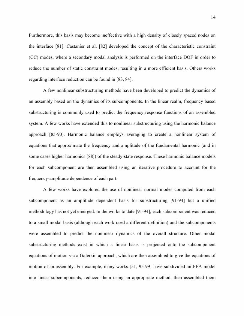
27

The initial conditions based on this static equilibrium become,

0

xz static,0

0 (14)

again assuming the initial velocities are set to zero. If static,0x were projected onto the linear

modes of the system, every modal amplitude may be nonzero. Similar to the EMD approach, the

rth NNM is initiated with only the rth modal coordinate in 0q set to a small value, as done with

Eq. (9). At low energy, the static deformation in Eq. (13) to an initial force profile defined by Eq.

(12) will result in a displacement field exactly in the rth linear mode shape. As the NNM branch

increases in energy, additional modes are added to the coordinate set as they are needed for

convergence of the shooting function, as explained later in Section 2.3.4.

2.3 Shooting and Pseudo-Arclength Continuation Algorithm

The pseudo-arclength continuation algorithm used here is essentially the same as that in

[49], but instead uses the EMD or AMF methods to reduce the number of variables to define the

initial displacements. These initial conditions greatly reduce the number of finite difference

computations required to estimate the Jacobian matrix used in the prediction and correction

steps. The mode augmenting scheme described in 2.3.4 is also novel to the pseudo-arclength

continuation algorithm presented in this chapter. The flow chart in Fig. 5 highlights the general

steps of the algorithm, and the details of the algorithm are presented in the following subsections.

28

Provide an initial guess for a periodic solution.

Extract linear normal modes from underlying linear equations.

Prediction Step: Tangent vector with step size

controller.

Correction Step: Newton-Raphson correction to update

initial conditions and period.

Mode Addition Criterion:Observe modal coordinates in time

history, add modes to coordinate set if needed for convergence.

Check Convergence:Integrate over one period.

)1()1(,0 , Tq

)1()1(,0 , jj Tq

)()1(

)()1(,0 , k

jk

j T q

Check Convergence:Integrate over one period.

Correction Step: Newton-Raphson correction to update

initial conditions and period. )(

)1()(

)1(,0 , kk Tq

YES NO

YES

NO

Provide an initial guess for a periodic solution.

Extract linear normal modes from underlying linear equations.

Prediction Step: Tangent vector with step size

controller.

Correction Step: Newton-Raphson correction to update

initial conditions and period.

Mode Addition Criterion:Observe modal coordinates in time

history, add modes to coordinate set if needed for convergence.

Check Convergence:Integrate over one period.

)1()1(,0 , Tq

)1()1(,0 , jj Tq

)()1(

)()1(,0 , k

jk

j T q

Check Convergence:Integrate over one period.

Correction Step: Newton-Raphson correction to update

initial conditions and period. )(

)1()(

)1(,0 , kk Tq

YES NO

YES

NO

Figure 5. Schematic of the AMF and EMD continuation algorithms to compute nonlinear normal modes.

2.3.1 Shooting Technique

The Newton-Raphson algorithm searches for solutions that satisfy the shooting function,

solving the two-point boundary value problem [45] of Eq. (5), and is defined as

0qzqzqH ),0(),(),( 0000 TT T (15)

29

The 12 N shooting function, ),( 0qH T , is converged with tolerance, , if the following

condition is satisfied.

),0(

),(

00

0

qz

qH T (16)

A Taylor series expansion of Eq. (15) is used to make corrections to the continuation

variables 0q and T in the event that Eq. (16) is not satisfied, just as done in [49]. The corrections

to the initial modal amplitudes and period ( 0q , T ) of the system generally satisfy the

algebraic equation,

),( 00

,,0 00

qHqH

q

H

qq

TTT TT

(17)

where the Jacobian is the )1(2 mN matrix on the left hand side of the equation. For the AMF

and EMD algorithms, the number of modal amplitudes is drastically smaller than the number of

physical DOF (i.e. mN ). The Jacobian is generated using a forward finite difference scheme,

requiring a total of m numerical integrations over a period T. The Jacobian is then transformed

into modal coordinates, reducing the size of the matrix in Eq. (17) from )1(2 mN to

)1(2 mm . This is accomplished by premultiplying both sides of Eq. (17) by the Nm 22

transformation matrix,

MΦ0

0MΦB

T

T

m

m (18)

where TmΦ contains the mass normalized mode shapes of the active modes as its rows. If the

mass matrix M is not available, a Moore-Penrose pseudo inverse can be used to invert the non-

30

square mode matrix. Premultiplying Eq. (17) by the transformation matrix B in Eq. (18)

eliminates any portion of the shooting function that is orthogonal to the m modes in the active

coordinate set, producing the following algebraic relation,

),( 00

,,000

qHqH

q

H

qq

TTT q

T

q

T

q

(19)

qH represents the shooting function in terms of the m modal coordinates active in 0q . The new

initial states and periods are updated using ( 0q , T ), providing the corrected initial modal

amplitudes and period as

)(

0)(

0)1(

0kkk qqq

(20)

)()()1( kkk TTT

(21)

The Jacobian matrix used in Eq. (19) is used throughout the prediction and correction steps that

follow.

2.3.2 Pseudo-Arclength Continuation: Prediction Step

The prediction step uses the last computed solution ( )(,0 jq , )( jT ) to estimate a prediction

vector TT)(,

T)(, jTjq PP tangent to the NNM branch, and is computed by solving the linear system

of equations defined as

0)(,

)(,

,,0)()(,0)()(,0

0PH

q

H

qq jT

jq

T

q

T

q

PTjjjj

(22)

31

where the Jacobian is the same as the one in Eq. (19). This requires m additional integrations of

the equations of motion over the period T about the last solution ( )(,0 jq , )( jT ). The normalized

prediction vector then uses the same step size control algorithm described by Peeters et al. to

obtain a prediction of the next solution as

)(,)()(,0)1(,0 jqjjj s Pqq (23)

)(,)()()1( jTjjj PsTT (24)

The step size controller, )( js , is determined by user defined inputs, such as the minimum and

maximum step size, as well as the ideal and maximum number of correction iterations as

described in [49].

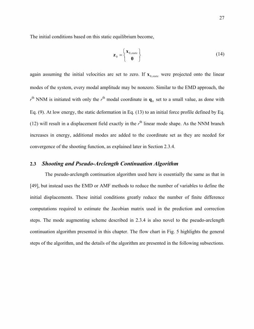
2.3.3 Pseudo-Arclength Continuation: Correction Step

The predicted solution )1(,0 jq is evaluated for periodicity over the period

)1( jT using the

shooting function in Eq. (15). If the periodicity condition is satisfied, then the solution is stored

and a new prediction is made from this new solution. If the shooting function is not satisfied,

then a corrector step is initiated using the Newton-Raphson approach to compute an update to the

modal amplitudes, )()1(,0

kjq , and period )(

)1(kjT , where k denotes the kth correction iteration. The

updates are computed using the Jacobian matrix in Eq. (19), with the added constraint that the

correction must be perpendicular to the prediction vector. This is accomplished by solving the

linear system of equations

0

),( )()1(,0

)()1(

)()1(

)()1(,0

)(,T

)(,

,,0 )()1(

)()1(,0

)()1(

)()1(,0

kj

kj

kj

kj

jTjq

T

q

T

qT

TP

T kj

kj

kj

kj

qHq

P

H

q

H

qq

(25)

32

The updated period and initial conditions are then computed using Eqs. (20) and (21). The

shooting function in Eq. (15) is evaluated for each correction step until convergence is met, at

which point the solution )1(,0 jq and )1( jT is stored and used to predict the next solution.

Because the nonlinearity essentially couples the underlying linear modes, additional modes

may begin to contribute to the response as the energy (or response amplitude) increases. These

modes, if not accounted for, may prevent the convergence of the shooting function within the

correction step of the algorithm. Therefore, an additional procedure is needed to detect modes

that may be important to obtain a periodic response, and add them when appropriate. Since the

size of the Jacobian in Eqs. (22) and (25) is governed by the number of active modal coordinates

m, it is preferable to include the smallest number of modes possible.

2.3.4 Add Linear Modal Coordinate

Within the correction step of the algorithm, the modes not included in 0q are monitored

with respect to their contribution to the shooting function in Eq. (15). The shooting function is

premultiplied by the transformation matrix B in Eq. (18) to filter modes only within the active

coordinate set, and then transformed back to physical coordinates, as follows

),(ˆ )()1(,0

)()1(

kj

kj

m

m T

qBH

Φ0

0ΦH (26)

The new shooting function, NR 2ˆ H , is used to determine whether the neglected modes prevent

convergence by evaluating the condition

),0(

),(ˆ

)()1(,00

)()1(,0

)()1(

kj

kj

kjT

qz

qH (27)

33

If Eq. (27) has converged to the desired numerical tolerance , but the full shooting function in

Eq. (15) has not, then a new mode is augmented to the modal variables as described in Eqs. (10)

and (11). To determine which mode to add, the shooting function is transformed into modal

displacements as

),( )(

)1(,0)(

)1(k

jkjq T qBH0IH

(28)

The maximum value of each modal coordinate in the shooting function is found and the most

dominant mode not currently in the variable set is added to the continuation variables. The

correction procedure is then resumed with m augmented by one. While this augmenting scheme

will allow the algorithm to converge to a periodic solution, experience has shown that modes

may be unnecessarily added. This tends to occur when the prediction step is somewhat far from

the NNM branch, or when finding an internal resonance that emanates from the backbone. Even

when this happens, the number of free variables is still greatly reduced relative to the original

algorithm, so this is not a large concern. One could add a condition to discard modes that are not

required for convergence, but this has not been pursued in this work.

2.3.5 FEA-Interface with NNM Algorithm

The AMF and EMD algorithms have been implemented in MATLAB®, and can interface

with many existing nonlinear finite element packages, which serve as a "black box" integrator for

the nonlinear system of interest. A schematic of the interface between the continuation algorithm

and the finite element software package is shown in Fig. 6. In this dissertation, only geometric

nonlinearities are considered, but other nonlinearities, such as contact and material nonlinearity,

could be accommodated as long as the equations of motion are conservative. The initial

conditions, 0z , are input to the finite element model from the continuation algorithm and

34

integrated by finite element code over a desired period T. The time histories of the response are

exported back into MATLAB for further evaluation (e.g. determining whether 0q and T satisfy

the shooting function). The time history data is written to a text file from the finite element

package, which is then read into MATLAB for evaluation. A more intrusive approach could be

used without reading/writing text files, and would likely improve the efficiency of the NNM

algorithm. This was not implemented for the results throughout this work, so the computational

times presented reflect a conservative number.

AMF or EMD Continuation Algorithm

Requirements:

-Read/Write to finite element package.

-Linear modes, time histories of free response, static deformations.

Compute linear(ized) mode shapes and

natural frequencies.

Write time history of free response to

computing environment.

Load model and specify initial

conditions and period of integration.

Integrate free response of finite element model.

Computing Environment Commercial FEA Package

Nonlinear static deformation to force profile (AMF only).

T,0z

tz,

Figure 6. Schematic of interface between computing environment and commercial finite element

package.

The nonlinear normal modes of two geometrically nonlinear finite element models were

computed using the proposed EMD and AMF strategies. The nonlinear modes are presented on a

two dimensional frequency-energy plane, where each point along the curve represents a free

35

periodic response exactly satisfying the full order finite element model. The fundamental

frequency of the response is plotted along the vertical axis, while the total conserved energy

(kinetic plus potential) of the response is on the horizontal axis. The results from a geometrically

nonlinear clamped-clamped beam are presented first, followed by a more realistic model of an

exhaust cover plate.

2.4 Application to Clamped-Clamped Beam with Geometric Nonlinearity

The EMD and AMF algorithms were applied to a finite element model in Abaqus® of a

clamped-clamped beam with geometric nonlinearity. The model was constructed using forty B31

beam elements, resulting in a total of 117 DOF. The B31 element is a 2-noded 3-D Euler-

Bernoulli beam that uses linear interpolation between each node. The out of plane z

displacement, and x and y rotations were fixed to model the beam as planar. The beam was 9

inches (229 mm) long, 0.5 inches (12.7 mm) wide and 0.031 inches (0.787 mm) thick. It was

constructed of structural steel with a Young's modulus of 29,700 ksi (204.8 GPa), shear modulus

of 11,600 ksi (80.0 GPa) and mass density of 7.36·10-4 lb-s2/in4 (7,870 kg/m3). The model

geometry was adopted from [19, 23, 108], where the beam served as a benchmark to validate a

variety of nonlinear model reduction strategies. The full, mass normalized mode matrix was

extracted using Abaqus’ Lanczos eigensolver. Abaqus directly integrated the free response to a

prescribed initial condition determined by 0q using its implicit Newmark-Beta scheme. The

average acceleration method was used with integration parameters γ=0.5 and β=0.25 [28], such

that algorithmic damping was not introduced into the time response. A suitable time step was

required to accurately capture the higher order harmonics of the response introduced by the

geometric nonlinearity. For the results shown this was accomplished by using 500 equidistant

time steps over one period of integration.

36

The first nonlinear normal mode of the beam was computed using the EMD and AMF

approaches with a shooting tolerance set to =10-4, and is shown in Fig. 7. Since the backbones

were of primary interest, a large maximum step size was used in the continuation algorithm in

hopes of "skipping" over any internal resonances that emanate from the backbone (a more

detailed NNM is presented later in Fig. 8). These results were used to evaluate the mode

augmenting scheme. At low energy, each branch was initiated with only the first linear bending

modal coordinate in the variable set. As the amplitude of the periodic response increased, more

modes were added to the modal set in order to satisfy the shooting function to the given tolerance

(these are marked with a star or triangle for the AMF and EMD methods, respectively).

10-6

10-5

10-4

10-3

10-2

10-1

80

100

120

140

Fre

que

ncy,

Hz

Applied Modal Force

10-6

10-5

10-4

10-3

10-2

10-1

80

100

120

140

Energy, in-lbf

Fre

que

ncy,

Hz

Enforced Modal Displacement

Figure 7. Frequency-energy plot of the first nonlinear normal mode of a geometrically nonlinear

beam. (Star) and (triangle) represents an added mode for the AMF and EMD method, respectively. (Note that 1 in-lbf = 0.113 N-m.)

37

The frequency-energy plots (FEPs) produced by the EMD and AMF methods were

indistinguishable, which was evident when the two branches were overlaid on the same plot (not

shown here for brevity). This is expected since the only difference was the method used to

determine the initial conditions; the solutions found by both algorithms satisfy the same shooting

function to the same tolerance when integrated with the same finite element model. There was a

significant difference in computational cost between the two approaches, however. For the

branches in Fig. 7, the AMF algorithm took a little over two hours to compute, while the EMD

approach took about 8 hours on a desktop computer with 8 GB of RAM and an Intel® Core i7

CPU. Tables 1 and 2 show the resulting modes that were added to the modal coordinate set as the

energy in the NNM 1 branch increased. For a frequency shift of ~77%, the AMF only required a

total of 4 modes, while the EMD method needed 18 modes. For either algorithm this represents a

significant reduction in the number of variables required to define the initial conditions for the

continuation algorithm, compared to the 117 DOF that define each physical displacement and

rotation of the model. The significance of this reduction comes through the cost required to

compute the Jacobian matrix, which requires a finite difference calculation (one period of

integration of the full finite element model) for each variable at every prediction/correction step.

Table 1. Modes added to NNM 1 using Applied Modal Force.

Frequency, Hz 79.4 95.9 121.9 Mode Added 3 5 7

Table 2. Modes added to NNM 1 using Enforced Modal Displacement.

Frequency, Hz 79.1 79.4 79.9 80.8 87.9 Mode Added 3 5, 39 7, 26 9, 45 11

Frequency, Hz 99.3 108.8 115.4 120.9 136.3

Mode Added 17, 47 20 49 22 24, 27, 51,

53

38

It is important to note that AMF adds extra computational cost compared to EMD since a

nonlinear static solution is required each time the model is integrated. For the beam studied here,

each static solution took about 10 seconds, while the numerical time integration over one period

took approximately 30 seconds. This 10 second increase from the nonlinear static solution was

far outweighed by the fact that AMF only had to iterate on 4 modes compared to 18 for the EMD

algorithm. For models with geometric nonlinearity, the quasi-static bending-axial coupling for

flat structures caused a stiffening effect as bending motions increased in amplitude. This was

implicitly captured by the preliminary static equilibrium solution of the AMF method. For

example, when a force was applied to the structure in the shape of only the first bending mode

using Eq. (12), other modes would be "statically" coupled to the response. When projecting this

static response onto the linear modes, the first mode would dominate the displacement, but other

modes would be implicitly present as well. The 26th and 39th axial vibration modes (along with

other bending modes) showed up in the response, as these were needed to relax the axial

deformation caused by the first bending mode shape. As a result, no axial modes were needed

within the AMF basis during the computation of the first NNM. The EMD method added seven

axial modes (26, 39, 45, 47, 49, 51, 53) to define the initial axial deformation for the first NNM.

The AMF needed fewer bending modes than EMD (4 compared to 11) as well, implying that

coupling between bending modes was also implicitly accounted for through the preliminary

static equilibrium.

The first three NNMs were computed with the AMF approach using a smaller maximum

step size in order to more completely resolve the branches. (The same computation would have

been much more expensive with the EMD approach so it was not pursued here.) A smaller

maximum step size improved the ability of the continuation algorithm to capture the internal

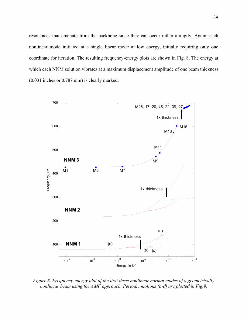
39

resonances that emanate from the backbone since they can occur rather abruptly. Again, each

nonlinear mode initiated at a single linear mode at low energy, initially requiring only one

coordinate for iteration. The resulting frequency-energy plots are shown in Fig. 8. The energy at

which each NNM solution vibrates at a maximum displacement amplitude of one beam thickness

(0.031 inches or 0.787 mm) is clearly marked.

10-5

10-4

10-3

10-2

10-1

100

100

200

300

400

500

600

700

Fre

quen

cy, H

z

Energy, in-lbf

1x thickness

1x thickness

(a)

(d)

(b) (c)

M1 M5 M7

M9

M11

M13M15

1x thickness

M26, 17, 20, 45, 22, 39, 27

NNM 3

NNM 2

NNM 1

Figure 8. Frequency-energy plot of the first three nonlinear normal modes of a geometrically

nonlinear beam using the AMF approach. Periodic motions (a-d) are plotted in Fig.9.

40

Each color section of the FEPs in Fig. 8 represent a portion of the NNM that was

continued from a new initial guess )1(,0)1(,0 ,Tq . Each new portion of the branch required either

an adjustment of the maximum prediction step size in order to more efficiently continue along an

internal resonance, or a change in the direction of the prediction step. For example, the black

curve of the NNM 2 branch started at low energy with a single mode, continued along the

backbone and followed the first internal resonance. The algorithm was then manually terminated

since the prediction step size was being reduced dramatically, and many modes were being

added to satisfy convergence. A new solution was then initiated on the backbone, right before the

tongue, with a large prediction step in order to find a new solution on the backbone beyond the

first internal resonance. From that new point, the prediction step was reversed with a smaller step

size, and the red curve was computed to resolve the internal resonance from the other direction.

It would have been ideal to capture the entire NNM branch in one computation, but it seemed

that when using Abaqus as the integrator (rather than MATLAB as done in [49]) it was not

possible to integrate with high enough accuracy to capture the ‘turn’ (fold bifurcation) at the end

of the tongue. This strategy was relatively manual, and required that the user adjust the

continuation settings (such as step size controller, etc.). In some cases it was observed that the

pseudo-arclength continuation algorithm jumped from one branch to another. For example, the

red curve representing an internal resonance along NNM 1 in Fig. 8 eventually would jump to a

period multiple of the third NNM, where the response was integrated over 5 times the minimum

period. When this occurred, the algorithm would be manually terminated and initiated at a

different starting point.

The frequencies/energies where a mode was added for the computation of NNM 3 are

marked in Fig. 8 where, for example, the M1 marker implies that the first linear mode was added

41

to the continuation variable set. The third NNM required a total of 15 modes with AMF to

compute the branch up to 690 Hz, where continuation had followed a 5:1 internal resonance with

NNM 9 until the algorithm was manually terminated. Along the backbone, the AMF algorithm

automatically added only symmetric bending modes (1, 5, 7, 9, 11, 13, 15) to the basis, similar to

the result of NNM 1 in Fig. 7. At the internal resonance, a few axial modes were added to the

basis (such as modes 26, 45, 39). Due to the excessive number of modes added along the tongue,

it was expected that these axial modes were mistakenly augmented to the continuation variable

set when the algorithm was iterating to find a converged solution. While the add mode condition

did not seem to be robust around the internal resonances, there was still a significant reduction in

continuation variables to iterate on (15 variables compared to 117 with all physical DOF). This

same behavior was also observed for other internal resonances in the first and second NNM. It is

important to mention that for these NNMs, the excessive number of modes added along the

internal resonance were not needed to satisfy shooting when the branch returned to the backbone.

42

Figure 9. (Left column) Initial displacement shapes of clamped-clamped beam with increasing energy of discrete solutions along the NNM 1 branch marked with (*) in Fig. 8. The color bar

gives the ratio of in-plane displacement to transverse displacement at each point along the beam. (Right column) The time histories show the nonlinear response projected onto the first 5

symmetric bending modes.

A few of the solutions on the first nonlinear normal mode at the points marked with an

asterisk (*) in Fig. 8 are plotted in Fig. 9, showing the nature of the periodic response at these

43

points along the branch. At low energy, the time history and initial deformation of solution (a)

was dominated by the first bending mode, and other modes had little contribution to the

response. At a higher energy along the backbone, solution (d) shows a large shift in frequency,

and higher order modes (mode 3 in particular) were clearly active in the time response, although

the initial deformation mode shape has not changed dramatically. The initial deformation shapes

reveal that the beam was deforming axially (the colorbar represents the ratio of axial to

transverse displacement for each node) in order to obtain a free response that satisfied the

shooting function at higher energy. The two solutions representing an internal resonance

(solutions (b) and (c)) show the interaction between higher order modes that can only be

explained with nonlinear normal mode theory. The time histories reveal that solution (b) is a 5:1

resonance with the third nonlinear mode, while solution (c) is a 12:1 internal resonance with the

fifth nonlinear mode.

2.5 Application to Exhaust Cover Panel with Geometric Nonlinearity

The applied modal force algorithm was also used to compute the NNMs of a

geometrically nonlinear finite element model of an exhaust cover plate, as a first step in

diagnosing unexplained failures that had occurred in operation. Swept sine tests on a large shaker

revealed that the frequencies of several of the resonances shifted significantly at the force levels

of interest, and this was likely caused by geometric nonlinearities. The plate has a diameter of

12.5 inches (317.5 mm), with a uniform thickness of 0.06 inches (1.5 mm), and was modeled in

Abaqus® with 899 S8R shell elements. The S8R element is an 8-noded thick shell element with

reduced integration and shear flexibility. The mesh for this model is shown in Fig. 10 where

there were a total of 15,708 DOF. Each element had the material property of structural steel with

a mass density of 7.29·10-4 lb-s2/in4 (7,800 kg/m3) and a Young's modulus of 30,200 ksi (208

44

GPa). The entire bottom ring of the plate was fully constrained (i.e. all 6 DOF fixed), as if the

plate were rigidly welded to an adjacent structure.

Figure 10. Finite element model of a geometrically nonlinear exhaust cover plate.

The FEP of the first NNM is plotted in Fig. 11, showing a frequency shift of 41% over

the computed branch. The value for the shooting function tolerance was set to =10-4, with the

same integration scheme and time steps used with the clamped-clamped beam in the previous

section. A total of 500 modes were extracted from Abaqus, which could be added to the

continuation variable set to define the initial conditions with the AMF approach. Each time

integration (over one period) with this model took about 700 seconds, and every static solution

took approximately 20 seconds. The total computational time for the FEP in Fig. 11 was

approximately 4 days on the desktop computer mentioned earlier. As discussed in Section 2.3.5,

this computational cost is conservative since the time histories were imported into MATLAB by

reading/writing text files, which added some cost to the algorithm.

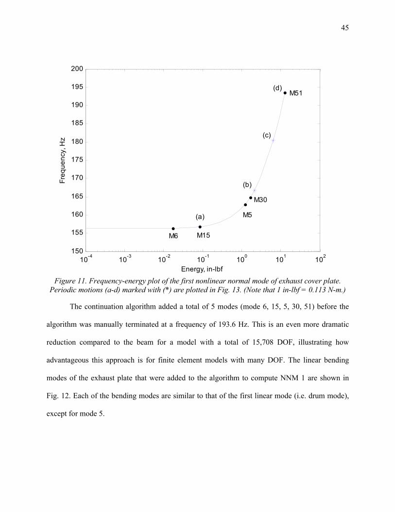
45

10-4

10-3

10-2

10-1

100

101

102

150

155

160

165

170

175

180

185

190

195

200

Energy, in-lbf

Fre

qu

en

cy, H

z

(b)

(c)

(d)

(a)

M6 M15

M5

M30

M51

Figure 11. Frequency-energy plot of the first nonlinear normal mode of exhaust cover plate.

Periodic motions (a-d) marked with (*) are plotted in Fig. 13. (Note that 1 in-lbf = 0.113 N-m.)

The continuation algorithm added a total of 5 modes (mode 6, 15, 5, 30, 51) before the

algorithm was manually terminated at a frequency of 193.6 Hz. This is an even more dramatic

reduction compared to the beam for a model with a total of 15,708 DOF, illustrating how

advantageous this approach is for finite element models with many DOF. The linear bending

modes of the exhaust plate that were added to the algorithm to compute NNM 1 are shown in

Fig. 12. Each of the bending modes are similar to that of the first linear mode (i.e. drum mode),

except for mode 5.

46

Figure 12. Linear (a) mode 1, (b) mode 5, (c) mode 6, (d) mode 15, (e) mode 30, and (f) mode 51

of exhaust cover plate that was added by the continuation algorithm to compute NNM 1. The color bar gives the amplitude of the out of plane displacement at each node.

The solutions marked with a (*) in Fig. 11 represent four discrete periodic solutions,

whose initial deformations are plotted in Fig. 13. The color bar in Fig. 13 represents the ratio of

the axial deformation at each node relative to the transverse displacement along the top of the

plate. The deformation shapes highlight the importance of the axial deformation in the initial

conditions of the NNM as energy increased. At low energy, the plate bends with little

accompanying axial stretch (Fig. 13a), about as much that is included in the first linear bending

mode. Experience with the EMD algorithm revealed that axial deformation must be considered

to compute the NNM out to a point where the natural frequency has shifted by less than 1%.

More stretching was observed as energy increased, with the largest tension towards the outer

edge of the plate. It is interesting to note how the deformations in Fig. 13(c) and (d) show the

presence of the 6th linear bending mode in initial displacement. The other modes (15, 5, 30, 51)

47

are needed to satisfy the shooting function but their effect is not pronounced in the initial

deformation shape. All of the modes required by the AMF algorithm were bending modes, as the

membrane effects of the nonlinearity were implicitly included by first solving the static

equilibrium problem. Based on the shape of the 5th bending mode, it is likely that this was

unnecessarily added, but this was not a concern since the algorithm still provided a drastic

reduction.

Figure 13. Initial displacement shapes of exhaust cover plate with increasing energy of discrete solutions along the frequency-energy plot in Fig. 11. The color bar gives the ratio of in-plane

displacement to transverse displacement at each point along the plate.

The EMD approach would have required more modes, likely both axial and bending as

seen with the clamped-clamped beam, in order to capture the deformations in Fig. 13. On the

desktop computer mentioned earlier, one Jacobian of the exhaust plate model would take about

48

135 days with the approach in [49] (with all 15,708 DOF), whereas the Jacobian with the AMF

approach (using 6 modes) took only 72 minutes. Each solution needed on average of 2-3

iterations within the correction step, and 1 prediction step (resulting in 3 to 4 Jacobian

computations per solution). The AMF algorithm has a clear advantage for the computation of

NNMs from finite element models with many DOF.

2.6 Summary

This chapter presented two numerical continuation approaches that can be used to

compute the nonlinear normal modes of structures modeled in commercial, geometrically

nonlinear finite element codes. These algorithms are an extension of the pseudo-arclength

continuation algorithm developed by Peeters et al. [49] with two major differences. First, two

approaches are used (AMF and EMD) to define the initial conditions based on a small subset of

the underlying linear modal coordinates, resulting in a dramatic reduction in the number of

variables that were varied within the continuation algorithm. Second, an add mode condition is

included to automatically add modal coordinates to the reduced coordinate set as they are needed

to satisfy convergence of the shooting function to a given numerical tolerance. The clamped-

clamped beam example in Section 2.4 showed a reduction from 117 DOF down to 4 DOF, and

18 DOF, respectively, for the AMF and EMD approaches. Furthermore, for the higher fidelity

model of the exhaust plate in Section 2.5, only 6 modal coordinates were required with AMF

compared to the 15,708 DOF that define the full order model, corresponding to almost a 3,000

fold decrease in the number of times that the response had to be integrated over one period at

each iteration.

One interesting discovery with the two algorithms is that only a few linear modal

coordinates were required to compute the nonlinear normal modes of these geometrically

49

nonlinear systems out to a significant shift in frequency. (In both cases, the NNMs were

computed out to a frequency shift similar to the amount observed experimentally [35, 109, 110].)

Even though the nonlinearity essentially couples all the underlying linear modal coordinates,

only a few of these are important to compute the nonlinear normal modes. These solutions

provide insight into which modes would be important to include in the kinematics of a reduced

order model. The NNMs of the full order model are used throughout this dissertation to validate

reduced models, providing a metric for comparison that is a unique signature of the nonlinear

system.

50

3 Geometrically Nonlinear Reduced Order Models

3.1 Introduction

This chapter reviews two indirect methods in the literature that generate reduced order

models of geometrically nonlinear finite element models built directly within commercial FEA

packages, as reviewed in [23, 24]. These methods project a set of Ritz vectors, or component

modes, onto the nonlinear FEA equations of motion to obtain a set of low order, nonlinear modal

equations. In commercially available FEA software, the linear mass and stiffness matrices can be

readily exported, however the nonlinear stiffness terms due to geometric nonlinearity cannot.

Therefore, an indirect approach is needed to estimate the nonlinear portion of the modal model

(i.e. a quadratic and cubic polynomial function of modal coordinates) using a series of static load

cases with either the applied loads procedure [19, 69, 103] or enforced displacements procedure

[62, 72]. The resulting modal model offers significant computational savings for time response

prediction compared to the direct integration of the full order model. Several existing works to

date have reduced the monolithic FEA model with its linear vibrations modes [23, 62, 64, 65, 67,

69, 72], although with enforced displacements procedure, sometimes this basis can be augmented

with a set of dual [67] or companion [23, 63] modes to capture in-plane kinematics.

These indirect nonlinear reduced order modeling (NLROM) strategies have been found to

be sensitive to several factors such as the amplitudes of the loads used to fit the nonlinear

stiffness coefficients, or the type and number of modes included in the basis. The inaccuracies of

the resulting fit may only be visible at certain response levels due to the amplitude dependence of

the NLROM. Relatively few works discuss the difficulties that can be encountered when seeking

an accurate modal model, so this chapter comprehensively reviews all of the decisions that go

51

into the ROM, and how these models are used in the NNM framework. Past works have

validated NLROMs experimentally or numerically by comparing time responses or the power

spectrum of the response to a random input [19, 66, 108, 111]. Throughout this dissertation, the

NNMs computed from candidate NLROMs generated with either the ED or ICE method are

compared to the NNMs of the full order FEA model, which are computed using the applied

modal force (AMF) algorithm in Chapter 2. The NNM offers a powerful metric to compare full

and reduced order models since these solutions span a range of response amplitudes and are

independent of any external forces.

3.2 Reduced Order Model Equations of Motion

The discretized system of equations for an N degree-of-freedom linear elastic,

geometrically nonlinear finite element model can be written as

tNL fxfKxxM

(29)

where M is the NN mass matrix, K is the NN linear stiffness matrix, xf NL is the 1N

nonlinear restoring force vector, and tf is the 1N external force vector. The 1N vectors x

and x are the displacement and acceleration, respectively. The NLROM procedures seek to

reduce these undamped, nonlinear equations using the linear vibration modes as the reduction

basis, which are found by solving the eigenvalue problem rr φMK 2 . A small set of mass

normalized mode shapes approximate the kinematics of the EOM as,

tt mqΦx

(30)

52

Each column in the mN mode shape matrix, mΦ , is a mass normalized mode shape vector, φ ,

and q is an 1m vector of time-dependent modal displacements. The vectors in mΦ are

truncated to a small number of mode shapes (depending on the NLROM strategy used) such that

the reduced coordinate space q is significantly smaller that the physical coordinate space x (i.e.

m << N).

In order to reduce the full order equations of motion (EOM), the transformation in Eq.

(30) is substituted into the full order EOM in Eq. (29) and premultiplied by TmΦ to assure that the

residual error is orthogonal to the reduction basis (note that ( )T is the transpose operator). The

reduced, nonlinear modal form of the rth equation becomes

tqqqqq rmrrrr fφT

212 ,,,

(31)

where r is the linear natural frequency, and rq is the rth modal displacement. The rth nonlinear

modal restoring force is given as

qΦfφq mNLrr

T (32)

The nonlinear restoring forces are a nonlinear function, qr , of the modal

displacements. Prior works [23, 24] have shown that if the finite element model is linear elastic

with geometric nonlinearities derived using quadratic strain-displacement relationships, the

function qr has the form of a quadratic and cubic polynomial given as

m

i

m

i

m

ijkji

m

jkrji

m

ijrmr qqqkjiAqqjiBqqq

1 121 ),,(),(),,,( (33)

53

The coefficients rB and rA are the quadratic and cubic nonlinear stiffness coefficients,

respectively, for the rth nonlinear modal equation. If the full order EOM in Eq. (29) is known in

closed form, then the nonlinear coefficients in Eq. (33) can be directly computed (referred as

direct evaluation in [23]). However, this work is interested in models where the closed form

equations are not explicitly available (e.g. within commercial finite element packages), and an

indirect approach must be used. The coefficients are estimated using either the enforced

displacements or Implicit Condensation and Expansion methods (otherwise known as the applied

loads method) using a series of nonlinear static solutions of the full order model. Once these

nonlinear stiffness terms are identified, the NLROM equations are completely given by Eqs. (31)

and (33), which can be used for time response prediction at a significantly lower cost than

compared to direct time integration of the full order model.

For the two NLROM methods discussed in this chapter, the linear term was set to 2r and

treated as a known value during the identification of rB and rA . Originally, McEwan used a

regression analysis to solve for the nonlinear stiffness coefficients using a set of applied load

cases [69]. Further development of the Implicit Condensation method led Gordon and Hollkamp

[19] to develop a constrained method where the nonlinear stiffness coefficients are directly

solved with a least squares approach while enforcing certain relations between some of the rB

and rA terms in order to preserve symmetry in the nonlinear stiffness matrices. This constrained

approach is used in the results in Chapter 4 to determine the nonlinear coefficients for the ICE

procedure, whereas the approach developed by Muravyov and Rizzi in [62] is used with the ED

method.

54

3.3 Identification of Nonlinear Stiffness Coefficients

3.3.1 Enforced Displacements Procedure

The enforced displacements procedure uses a set of prescribed displacements that are in a

permutation of the sums and differences of either one, two or three of the mode shapes in the

basis in Eq. (30). In general, the cth multi-modal displacement combination of the rth, sth, and pth

modes can be written as

ppssrrc qqq ˆˆˆ φφφX (34)

The 1N displacement vector cX is an enforced displacement field applied to the full order

model, and the q̂ 's are the prescribed scaling factors for each mode. In order to accurately

estimate the ROM, the scaling factors should scale the deformation shape of each mode to a level

that exercises the geometric nonlinearity in the structure. Using the static solver in the finite

element package, the resulting reaction force, cF , is computed in response to the cth displacement

field, cX . The estimation procedure in [62] uses a series of these enforced displacement fields

that are in various combinations of one, two or three modes in the basis set. These displacements

and the resulting reaction forces are used to identify the nonlinear stiffness coefficients from the

quasi-static representation of the NLROM, where the rth modal equation is given as

m

icr

m

i

m

ijkji

m

jkrji

m

ijrrr qqqkjiAqqjiBq

1 1

2 ˆˆˆ),,(ˆˆ),(ˆ FφT (35)

The number of nonlinear static solutions, for m > 3, required by the ED method [24] is

)!3(6

!

)!2(2

!32

m

m

m

mm (36)

55

3.3.2 Applied Loads Procedure or Implicit Condensation and Expansion

The applied loads procedure is conceptually similar to the ED approach, but instead uses

a set of static forces that are in a permutation of the sums and differences of either one, two or

three of the mode shapes in the basis in Eq. (30). A multi-mode static force for the cth load case

can be written as a combination of the rth, sth, and pth modes as

ppssrrc fff ˆˆˆ φφφMF

(37)

where cF is the 1N vector of static forces applied to the FEA model, and the f̂ 's are the force

scaling factors for each mode. Note that existing works on the applied loads method do not

mention the use of the mass matrix when computing the static force vector, cF , but it was used

here and is needed to obtain a force that exactly isolates a single mode for a linear system (e.g.

when 0xf NL in Eq. (29)). The force scaling factors should be selected to exercise the desired

amount of geometric nonlinearity in the structure, as will be discussed further in Section 3.5. The

resulting static deformation, cX , computed from the FEA static solver in response to the cth

static force, cF , is then projected onto each of the linear modal coordinates in the basis as

follows

crrq MXφT (38)

Using a series of these applied forces and displacements, one can use the quasi-static form of the

NLROM in Eq. (35) to solve for the nonlinear stiffness coefficients with the constrained least

squares estimation procedure in [19]. With the applied loads approach, the number of load

permutations (for m > 3) required to generate the static response data [19] is given as

56

)!3(3

!4

)!2(

!22

m

m

m

mm (39)

Regardless of the estimation procedure used to identify the nonlinear stiffness

coefficients, there are many user decisions that are made by the analyst when creating these

models. Inputs such as mode selection and static load scaling factors greatly affect the accuracy

of the resulting NLROM, and are exploited when comparing the nonlinear normal modes

computed from these reduced equations. Previous works [19, 62] have provided basic guidelines

for the model reduction procedure, and many of these guidelines are comprehensively discussed

below.

3.4 Mode Selection

It is imperative to include all of the dynamically important modes in the reduced basis in

Eq. (30) when creating the reduced order model, otherwise the NLROM will not be adequate for

its intended purpose. For a linear system, one typically includes all of the excitable modes in a

frequency range of interest to accurately capture the response of the model, however the addition

of geometric nonlinearity requires further considerations. For example, the nonlinearity

essentially couples the underlying linear modes of the structure, so additional modes outside the

typical bandwidth of interest may be needed to account for such interactions. A low frequency

mode can potentially excite a higher frequency mode outside of the desired excitation bandwidth

and if the coupling is strong, these high frequency modes should be included in the basis set. For

example, if the structure’s nonlinearity is cubic, then it is well known that a periodic input at a

frequency may excite modes at higher harmonics such as 3, 5 and hence one may need to

consider modes outside the bandwidth of the input forces to accurately capture the response of

the structure.

57

The method used to estimate the NLROM coefficients (either ED or ICE) also has a

strong influence on which modes to include. For example, the coupling between the bending and

membrane motions cause "stretching" that is not always accurately captured with a set of low

frequency bending modes. When using the enforced displacements procedure, high frequency

membrane/axial modes must be explicitly included in the basis to account for the coupling. On

the other hand, with the Implicit Condensation and Expansion method, membrane modes do not

need to be included since the softening due to membrane stretching is implicitly captured during

the identification of the nonlinear stiffness coefficients. Nonlinear systems are also known to

exhibit modal interactions, where an NNM at a given energy level can exchange energy with a

different NNM [25, 38]. In order to capture this phenomena, the NLROM must include the mode

shapes/kinematics that are involved in the modal interaction. In theory, an infinite number of

interactions may exist for even the simplest systems, but certain ones may likely be more

important than others.

A few methods have been proposed to identify a sufficient modal basis for the NLROM.

For example, Rizzi and his colleagues presented an approach in [66, 111] that uses a short

dynamic response to a representative loading to determine which modes significantly contribute

to that response. This dissertation proposes an alternate approach to identify which modes are

nonlinearly coupled to each of the bending modes of interest based on nonlinear static solutions.

A force proportional to a single, linear mode shape, rφ , is scaled with a scale factor, rf̂ , which

is chosen to ensure the geometric nonlinearity is sufficiently excited (see Section 3.5.2). This

force is applied to the nonlinear FEA model and the nonlinear static response to the given force

reveals which axial and bending modes couple to the rth bending mode of interest. Specifically,

58

the FEA software solves the following static equation, where external force is applied in the

shape of the rth linear mode,

rrstaticNLstatic f̂MφXfKX

(40)

The displacement, staticX , resulting from the static force is then projected onto all the modal

coordinates as

staticMXΦq T (41)

If the force amplitude is too small (in the linear regime), the applied force will result in a

displacement exactly in the rth mode shape and hence only rq will be nonzero. For larger force

amplitudes, the nonlinear static solution reveals the natural coupling between that mode and

other bending and membrane modes due to the geometric nonlinearity. The modal amplitudes in

Eq. (41) guide the selection of the appropriate modes to supplement each linear mode that falls in

the frequency range of interest. Consider the computation of the rth nonlinear normal mode

initiated at the rth linear mode at low energy. The NNM can be checked for convergence by

adding the linear mode with the next largest value in the q vector in Eq. (41) to the NLROM

basis in Eq. (30) , and then recomputing NLROM and its NNM. If the additional mode improves

the resulting NNM, then that mode should be included in the basis set. This procedure helps

identify when a sufficient basis set has been selected to capture the rth NNM. This can be used

for both the ED and ICE procedures, and will be demonstrated throughout the results in Chapter

4.

59

3.5 Scaling Factors for Multi-Mode Models

The scaling factors on the static load cases in Eq. (34) for ED and Eq. (37) for ICE

govern the degree to which the nonlinearity in the FEA model is activated in the response data

used to fit the nonlinear stiffness coefficients. If the scale factors are too small, the nonlinearity

in the response may be on the order of computational noise leading to numerical difficulty when

attempting to determine the polynomial coefficients rA and rB . Similar problems may result if

one mode is excited far more or far less than the others. This section discusses the suggested

approaches for selecting the scale factors with the ED and ICE estimation procedures.

3.5.1 Enforced Displacement Scaling Factors

One scaling approach, termed the constant modal displacement (CD) factor, sets the

scaling factors, q̂ , in Eq. (34) for each mode in a meaningful way. The modal scale factor

required to displace the rth mode to a desired maximum displacement in physical coordinates,

rwmax, , can be written as

max,

max,ˆr

rrr

wCDq

φ (42)

The scalar max,rφ is the maximum displacement value (i.e. ignoring any rotations) of the rth mass

normalized mode shape in the basis. Note that generally the maximum displacement occurs at a

different displacement DOF for each mode, and that different values of rwmax, may be chosen

depending on the mode of interest. For example, if the scaling factor is for a bending mode,

choosing a rwmax, value on the order of the thickness of the structure will typically assure that the

displacements exercise the nonlinearity. For an axial mode, then a value on the order of a

60

fraction of the thickness (a tenth or hundredth) should be used since these modes do not behave

nonlinearly and unreasonably large forces would be needed to cause them to displace by one

thickness, possibly introducing numerical ill-conditioning into the estimation process.

The works in [62, 65] suggest that the ED NLROM obtained is theoretically insensitive

to the amplitudes of q̂ , however should be chosen to be physically reasonable and within the

range of interest. For the enforced displacement procedure, they proposed using the same scaling

factor for all modal displacements in Eq. (34). This method will be referred to as the constant

modal scale (CS) factor method, where the scale factors are determined based on the maximum

displacement of the lowest order bending mode as

1ˆ CDCSq rr (43)

where 1CD is given by Eq. (42). It is suggested that 1max,w is chosen to be physically reasonable

for the lowest frequency bending mode and within the range of displacements expected in the

application of interest. The results in Chapter 4 explore the results obtained by each approach

and discuss some of the issues that arise.

It is noted that Mignolet, Perez, Wang and others have also employed the enforced

displacements procedure successfully with many structures [24, 72, 102, 112]. They typically

set CDr for each mode such that each bending mode displaces 1.0 times the thickness and a

displacement < 1.0 times the thickness for the membrane/axial modes. The optimal CD values

are problem dependent and so they typically employ a few values near 1.0 thickness and check

whether the ROM coefficients vary significantly. They also typically use the "cleaning"

procedure described in [112] to zero out any cubic rA and quadratic rB terms involving only

one axial mode. Finally, it should be noted that their approach to determine the ROM

61

coefficients differs slightly from that outlined in this chapter; they estimate both the linear and

nonlinear stiffness coefficients in the ROM from the results of the static load cases (in this

dissertation, the linear terms were always set to 2r ). They compared the linear terms against the

known linear natural frequencies to check the consistency of the results; they may vary from the

linear natural frequencies if too large of loads have been applied. This approach was not

implemented in this work, but it should be kept in mind as it may explain some of the differences

between the scaling values that worked best in Chapter 4 and those reported in their works.

3.5.2 Applied Load Scaling Factors

For the applied loads procedure, Gordon and Hollkamp specify scaling factors based on

the amount of force required to achieve a certain maximum displacement for the linear system

[19]. The equation for the scaling factor of the rth mode shape based on the load case in Eq. (37)

is formulated as

2

max,

max,ˆr

r

rrr

wCLDf

φ (44)

This method of scaling is termed constant linear displacement (CLD). Note that this equation is

slightly different than the equation presented in [19] due to the mass matrix being pre-multiplied

by the force vector in Eq. (37). The desired linear displacement for each mode should

sufficiently excite the geometric nonlinearity. Typically a displacement on the order of one

thickness is used for the primary, low frequency modes [19], however, higher frequency modes

tend to require a lower rwmax, value. It is important to select a displacement amplitude, rwmax, ,

large enough to overcome the linear range of the response, but small enough to avoid

convergence issues with the finite element solution. One recommendation for determining rwmax,

62

for each mode is to compute the nonlinear static solution to the force in Eq. (40), and find the

resulting maximum nonlinear displacement, NLrw ,max, . The ratio of the nonlinear to linear

maximum displacement is defined as the ratio

r

NLrr w

w

max,

,max, (45)

Typically, the ratio for r should be between 0.8 and 0.95 for hardening nonlinearities, or 1.05

to 1.2 for softening nonlinearities [19].

Another important issue arises when determining the load cases that involve a

combination of two or three modes simultaneously. After determining the CLD scaling factors

for each mode in the basis, a reduction of these force amplitudes is recommended here. For

example, when applying a load in the combination of modes 1 and 2, the CLD factors should be

reduced by a factor of two such that the loading becomes

2211

ˆ2

1ˆ2

1ffc φφMF (46)

Similarly for combinations of three modes, each CLD factor should be reduced by a factor of

three. This ensures that the applied forces do not exceed desired displacement levels, and

contaminate the fit of the nonlinear stiffness coefficients. This method is termed the reduction

factor (RF) method.

3.6 Nonlinear Normal Modes of Reduced Order Models

Once the NLROM equations are identified using either parameter estimation procedure,

the NNMs of the modal equations are computed using the pseudo-arclength continuation

algorithm in [49]. From the equations of motion in Eqs. (31) and (33), there exist at least m

63

nonlinear normal modes that are extensions of the linear modes in the basis. The continuation

algorithm uses the linear mode solution at low response amplitude as an initial guess, and the

predictor-corrector type algorithm traces the periodic solutions as the response amplitude

increases. The method relies on the shooting technique to find the periodic solutions of the

equations of motion, using the shooting function

0

q

q

qqq

qqqqqH

0

0

00

0000 ,,

,,,,

T

TT (47)

A valid NNM is defined as a periodic motion with integration period T, initial modal

displacement 0q , and initial modal velocity 0q that satisfies the shooting function to a given

numerical tolerance. The algorithm in [49] iterates on these variables (T, 0q , 0q ) using a

Newton-Raphson method to search for a response that satisfies Eq. (47). Once a periodic solution

is found, the solution is stored and the algorithm predicts a new solution along a line tangent to

the current branch. The correction step is repeated by adjusting the predicted solution until the

shooting function is again satisfied.

One advantage to the numerical continuation approach is that it can handle strong

nonlinearities since each periodic solution is exact to a given integration tolerance.

Unfortunately, the cost of the algorithm grows in proportion to the number of DOF in the model.

NLROMs have the computational advantage of having far fewer DOF compared to the full finite

element model, making the NNM computation very efficient. Furthermore, the Jacobian of the

NLROM can be derived analytically from Eqs. (31) and (33), so the method in [49] is used to

further speed up the computations, compared to the finite difference approach used in Chapter 2.

Hence, this is a very efficient means of computing the NNMs of a geometrically nonlinear

64

structure, the only question is whether the NLROM is an accurate representation of the FEA

model of interest.

3.7 Expansion of In-Plane Displacements for Applied Loads

As stated earlier, the applied loads approach condenses the quasi-static membrane effects

induced by large bending amplitudes into the nonlinear stiffness coefficients of the modal

models. The advantage to this is that the membrane type modes do not need to be explicitly

included in the basis set, allowing for a lower order ROM. Membrane or axial modes typically

have much higher frequencies and require shorter time steps during numerical integration. When

recovering the displacements in physical coordinates using the modal coordinates in Eq. (30), the

transformation does not necessarily contain the correct membrane kinematics that are excited by

the bending-membrane coupling. Hence, those displacements cannot be used to recover accurate

stresses and strains from the FEA model as a post-processing step. Hollkamp and Gordon

developed a remedy by recovering these membrane motions when expanding back to physical

coordinates [103]. They estimate a set of membrane basis vectors that account for membrane

stretching, and are related to the physical deformations as functions of the bending modal

coordinates. Each modal model has its own unique set of expanded membrane basis vectors

depending on the bending modes used in the basis, and are only needed when recovering

physical displacements as a post-processing step.

The derivation of the expanded membrane motions from [103] is summarized here. The

transformation in Eq. (30) is augmented with membrane motions so it becomes

pTqΦx mm (48)

65

The kN matrix mT contains k membrane basis vectors, one in each column, and the 1k

vector p contains the generalized membrane coordinates. The membrane motions are found by

returning to the results of the static load cases performed to create the ROM. Each static

deformation, cX , to a modal force in Eq. (37) is assumed to be well approximated using the

expanded basis

pTqΦX mcmc

(49)

where cq are the modal amplitudes of each mode contributing to the response in cX computed

using the modal filter in Eq. (38). The entire series of static solutions used to fit the nonlinear

stiffness coefficients are considered simultaneously by collecting all columns of Eq. (49).

PTQΦX mmstatic

(50)

The columns of the matrices staticX , Q , and P represent the individual static solutions to the

load cases defined by Eq. (37). Assuming there are a total of l static load cases (see Eq. (39)), the

dimensions of each matrix are lN , lm , and lk , respectively.

It is assumed that the membrane basis vectors in mT are orthogonal to the mode shapes in

mΦ , allowing the modes to be projected onto the physical displacements as

staticmmm XΦΦΦQ TT 1

(51)

Note that the matrix, Q , can also be computed as staticmMXΦQ T if the basis in mΦ are linear,

mass normalized vibration modes. Assuming now that the generalized membrane amplitudes are

known, the membrane basis could theoretically be estimated from

66

1

TT PPPQΦXT mstaticm (52)

Following the approach developed in [103], a quadratic relationship is assumed between the

modal coordinates in q and the generalized membranes amplitudes p such that

T2

12

12322213121

21 mmmmmm qqqqqqqqqqqqqqqq p

(53)

The expanded membrane motions can now be estimated using Eqs. (51) to (53). Once a solution

to the NLROM in Eqs. (31) and (33) has been integrated, the resulting physical displacements

can be expanded as a post-processing procedure using Eq. (48) in order to accurately compute

the stress and strain in each finite element. These generalized membrane coordinates are not

included explicitly in the nonlinear differential equations, so there is no increase in order size of

the system being integrated.

67

4 Convergence Evaluation of Monolithic Nonlinear Reduced Order Models

4.1 Introduction

This chapter uses the nonlinear normal modes as a metric to determine the convergence

of a ROM either as modes are added to the basis, or as the amplitudes change on the static loads

used to identify the nonlinear stiffness coefficients. The enforced displacement and Implicit

Condensation and Expansion parameter estimation approaches are evaluated here on the two

geometrically nonlinear finite element models presented in Chapter 2. The first is a flat planar

beam with 117 DOF and clamped-clamped boundary conditions, while the second is a more

complicated FEA model of an exhaust cover plate with 15,708 DOF. The NLROMs were created

for each model with different modes and scaling factors, and then the NNMs were computed and

compared to gain insight into the convergence and accuracy of the models. These results are

compared with the true NNMs computed from the full order models using the applied modal

force (AMF) algorithm in Chapter 2. In practice, these solutions will not necessarily be available

since this truth data is computationally expensive, however the ROM can still be validated based

on how the NNMs converge as the modal models are refined. For the development of this

research, it is informative to have these reference NNMs from the full order model.

A third case study is presented in this chapter using a linear beam model with a local

contact nonlinearity modeled as a unilateral piecewise-linear spring. The reduced order models

of this system are generated using a Galerkin approach with linear vibrations modes augmented

with a single discontinuous basis function, as done in [113]. The NNMs are computed from a

candidate set of ROMs with a successively increasing number of vibration modes in the basis,

and the accuracy of the ROMs are evaluated based on the convergence of the resulting NNMs.

68

No reference NNMs were available from the full order model, so the effectiveness of the NNM

convergence metric is evaluated by comparing the response of the ROMs to the full order model

for both an impulsive load and a random input.

4.2 Application to Clamped-Clamped Beam with Geometric Nonlinearity

The beam model studied here was identical to that in [23], and had the following

dimensions: 9 inches (229 mm) long, with a cross section of 0.5 inches (12.7 mm) wide by 0.031

inches (0.787 mm) thick. It was modeled with forty B31 beam elements in Abaqus®, resulting in

117 DOF. It was constructed of steel with a Young's modulus of 29,700 ksi (204.8 GPa), a shear

modulus of 11,600 ksi (80.0 GPa) and a mass density of 7.36·10-4 lb-s2/in4 (7,870 kg/m3). The

geometrically nonlinear beam exhibited hardening nonlinearities, as shown in Chapter 2, due to

the coupling between bending and membrane motions at large response amplitudes.

First, the modal coupling due to the geometric nonlinearity was investigated by applying

a static force proportional to the first five symmetric bending modes, and projecting the

displacement onto the mass normalized linear modes using Eq. (41). As in [23], it was presumed

that the anti-symmetric modes will not be excited and hence are not of interest. The force was

scaled for each of the modes using the CLD method in Eq. (44) with a rwmax, value of 0.031

inches (0.787 mm), or 1 beam thickness. The magnitude of the resulting modal amplitudes were

normalized to the largest amplitude, and sorted in descending order in Table 3. An applied static

force meant to excite the first linear mode revealed nonlinear coupling to other symmetric

bending modes (modes 3, 5, 7, 9, etc..). In addition, anti-symmetric axial modes 26, 39, 45 and

47 were found to be coupled to it as well. The results suggest which axial/membrane modes to

augment with the bending modes for the ED procedure, as well as which bending modes to

69

successively include in the basis set for either the ED or ICE method in order to get convergence

of the NLROM.

Table 3. Relative modal amplitude due to a static force applied to excite the linear mode shapes of the clamped-clamped beam.

Force in Mode 1 Force in Mode 3 Force in Mode 5 Force in Mode 7 Force in Mode 9 Mode # Amp Mode # Amp Mode # Amp Mode # Amp Mode # Amp

1 1 3 1 5 1 7 1 9 1 3 9.3·10-3 1 5.7·10-1 1 6.8·10-1 1 7.2·10-1 1 7.4·10-1 5 1.3·10-3 5 2.4·10-2 3 2.0·10-1 3 2.6·10-1 3 2.9·10-1

39 5.0·10-4 7 7.2·10-3 7 2.6·10-2 5 1.1·10-1 5 1.4·10-1 7 3.1·10-4 9 2.7·10-3 9 1.1·10-2 9 2.5·10-2 7 7.6·10-2

26 2.4·10-4 47 1.5·10-3 11 5.3·10-3 11 1.3·10-2 11 2.3·10-2 9 9.9·10-5 11 1.1·10-3 13 2.7·10-3 13 7.1·10-3 13 1.4·10-2

45 6.7·10-5 45 9.8·10-4 51 2.6·10-3 15 4.1·10-3 15 8.2·10-3 11 3.9·10-5 13 5.5·10-4 49 1.9·10-3 55 3.6·10-3 17 5.1·10-3 13 1.8·10-5 49 4.1·10-4 15 1.5·10-3 53 2.9·10-3 59 4.7·10-3 47 1.7·10-5 15 2.9·10-4 26 1.1·10-3 17 2.5·10-3 57 3.9·10-3

4.2.1 One-Mode NLROMs

A one-mode NLROM was first generated using the ED and ICE procedures, and the

NNMs were computed from the resulting equations and are shown in Fig. 14. The CLD factor

was used with ICE, where the 1max,w value was set to a displacement of 0.5 times the beam

thickness, or 0.016 inches (0.394 mm). The ratio of nonlinear to linear displacement at the

midpoint with this scale factor was γ1=0.88. For the ED NLROM, a CD scale factor that

produced a maximum displacement such that 1max,w was 3 times the thickness was used. The

reason for selecting these optimal values is addressed later in this subsection. The legend for

each NLROM in Fig. 14 uses the following convention: "NLROM strategy (modes included)

scaling method ( rwmax, /beam thickness x Number of modes with that ratio)." For example, the

last line in the legend in Fig. 14 represents an enforced displacement NLROM (ED) which

includes modes 1, 26, and 39 using the constant displacement scale factor method (CD) with

70

1max,w set to 3 times the beam thickness for the first mode in the basis set (mode 1) and 26max,w

and 39max,w set to 0.01 times the beam thickness for the two (x2) axial modes (modes 26 and 39).

10-7

10-6

10-5

10-4

10-3

10-2

70

80

90

100

110

120

130

Energy, N-m

Fre

quen

cy,

Hz

AMF

ICE (1) CLD (0.5)

ED (1) CD (3.0)

ED (1 26 39) CS (3.0)

ED (1 26 39) CD (3.0 0.01 x2)

(a)

(b)

Figure 14. Frequency-energy plot of NNM 1 of the clamped-clamped beam model with various

NLROM strategies. Deformations of solutions (a) and (b) are plotted in Fig. 15.

The NNM is shown on the frequency-energy plane, where each point along the curve

represents a periodic solution to the nonlinear equations. The fundamental frequency on the

vertical axis was computed from the minimum period of the response (higher harmonics were

generally observed as energy increased). The energy along the horizontal axis was computed as

the total energy, kinetic plus potential, of the system during the periodic response. The results in

Fig. 14 show that a one-mode NLROM created using the ICE procedure (dashed red) accurately

captured the backbone of the first NNM when compared to the truth results from AMF (black

circles). At higher energies (above 0.003 N-m), the one-mode ICE NLROM was slightly stiffer

71

than the true NNM. As expected, a comparable one-mode model created using the enforced

displacement procedure (blue squares) was much stiffer and hence much less accurate than the

ICE NLROM over the whole energy range due to the lack of membrane-softening in the basis. It

is well known that membrane modes must be included in an ED NLROM in order to obtain

accurate results; the results above exploit the error that is incurred when the membrane modes

are neglected.

The ED NLROM was improved by adding the first two anti-symmetric axial modes to

the basis set (modes 26 and 39), as determined by the coupling in Table 3. Two different scaling

methods were used with the NLROMs that included these axial modes: CS scaling, and also CD

scaling with rwmax, set to 3 times and 0.01 times the beam thickness for the first bending mode

and the associated axial modes, respectively. After adding these two axial modes, either of the

ED NLROMs were as accurate as the one-mode ICE NLROM. This illustrates the fact that the

membrane displacements must be included in the basis set for the ED method in order to

accurately capture the nonlinear stiffness, whereas the ICE method implicitly captured these

effects. For this NNM no difference was seen between the results obtained using the CD (short

dashed green) and CS (dashed dot magenta) scaling methods. Hence, when using the enforced

displacements approach the higher frequency axial modes can be displaced much less than the

bending modes during the static load cases and produce an accurate NLROM.

All of these approaches gave an excellent estimate for the backbone of NNM 1, even

though the NLROMs only included the first bending mode. The ED procedure was at a slight

disadvantage since it required the axial modes explicitly in the basis set, but in this case these

modes were easily identified using a statically applied force in the shape of the first bending

mode as shown in Table 3. The dual modes method proposed by Kim, Mignolet et al. [67] would

72

likely include similar axial effects, but this basis was not explored in this work. Each NLROM

captured the bending-membrane coupling caused by geometric nonlinearity, and was examined

more thoroughly by looking at the physical deformations at different points along the NNM

branch. The plot in Fig. 15 shows the maximum deformation shape (e.g. when the velocity of the

periodic response was zero) at the points marked (a) and (b) in Fig. 14 for the ICE and ED

methods, as well as the AMF truth results (note that the expansion method in Section 3.7 had to

be used to capture the membrane deformations with ICE). The position of each node is plotted in

millimeters, and the color bar shows the log of the ratio of in-plane displacement to transverse

displacement at each node.

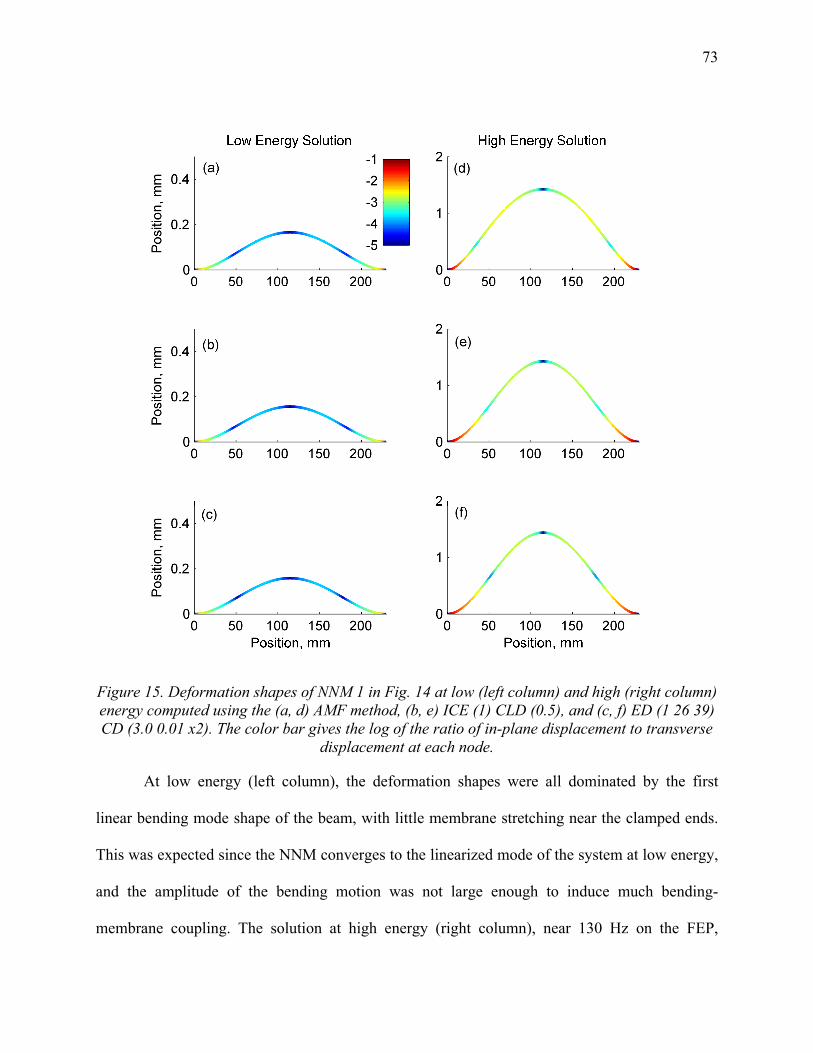
73

Figure 15. Deformation shapes of NNM 1 in Fig. 14 at low (left column) and high (right column) energy computed using the (a, d) AMF method, (b, e) ICE (1) CLD (0.5), and (c, f) ED (1 26 39) CD (3.0 0.01 x2). The color bar gives the log of the ratio of in-plane displacement to transverse

displacement at each node.

At low energy (left column), the deformation shapes were all dominated by the first

linear bending mode shape of the beam, with little membrane stretching near the clamped ends.

This was expected since the NNM converges to the linearized mode of the system at low energy,

and the amplitude of the bending motion was not large enough to induce much bending-

membrane coupling. The solution at high energy (right column), near 130 Hz on the FEP,

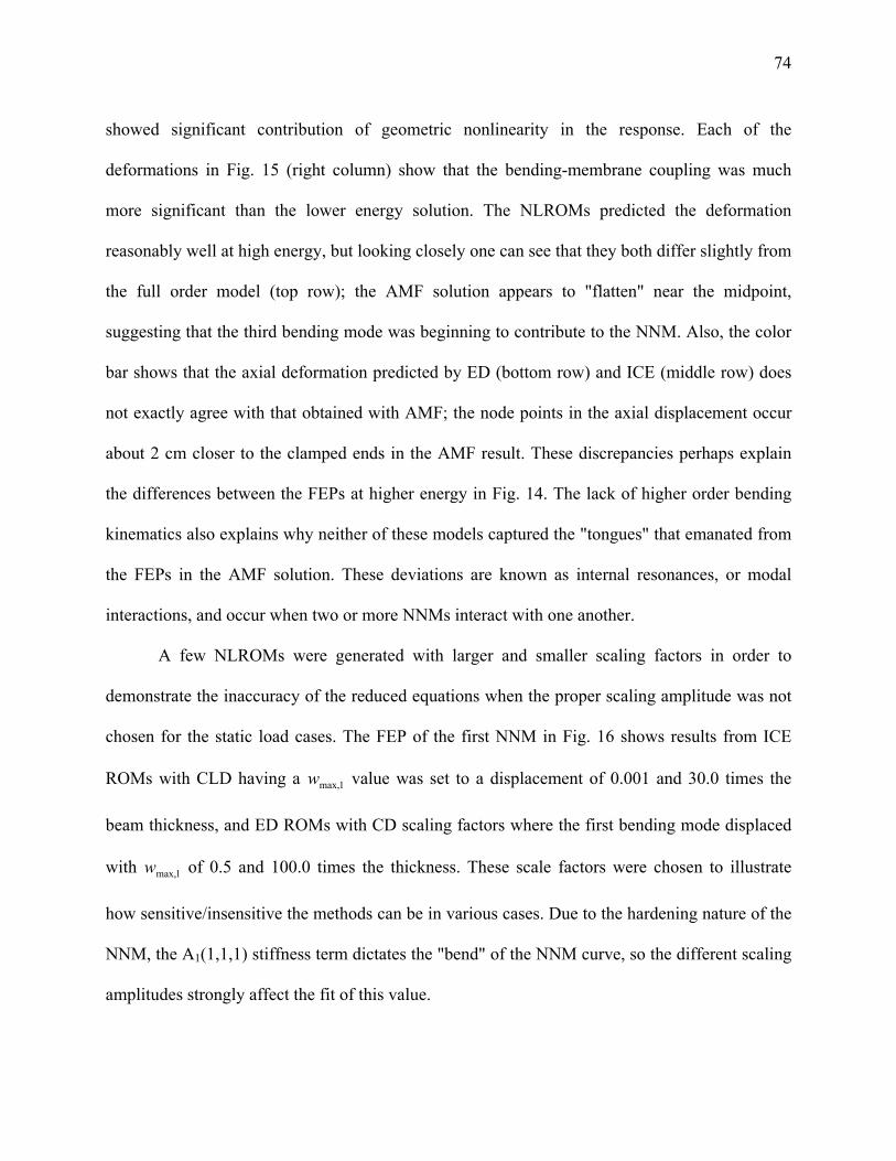
74

showed significant contribution of geometric nonlinearity in the response. Each of the

deformations in Fig. 15 (right column) show that the bending-membrane coupling was much

more significant than the lower energy solution. The NLROMs predicted the deformation

reasonably well at high energy, but looking closely one can see that they both differ slightly from

the full order model (top row); the AMF solution appears to "flatten" near the midpoint,

suggesting that the third bending mode was beginning to contribute to the NNM. Also, the color

bar shows that the axial deformation predicted by ED (bottom row) and ICE (middle row) does

not exactly agree with that obtained with AMF; the node points in the axial displacement occur

about 2 cm closer to the clamped ends in the AMF result. These discrepancies perhaps explain

the differences between the FEPs at higher energy in Fig. 14. The lack of higher order bending

kinematics also explains why neither of these models captured the "tongues" that emanated from

the FEPs in the AMF solution. These deviations are known as internal resonances, or modal

interactions, and occur when two or more NNMs interact with one another.

A few NLROMs were generated with larger and smaller scaling factors in order to

demonstrate the inaccuracy of the reduced equations when the proper scaling amplitude was not

chosen for the static load cases. The FEP of the first NNM in Fig. 16 shows results from ICE

ROMs with CLD having a 1max,w value was set to a displacement of 0.001 and 30.0 times the

beam thickness, and ED ROMs with CD scaling factors where the first bending mode displaced

with 1max,w of 0.5 and 100.0 times the thickness. These scale factors were chosen to illustrate

how sensitive/insensitive the methods can be in various cases. Due to the hardening nature of the

NNM, the A1(1,1,1) stiffness term dictates the "bend" of the NNM curve, so the different scaling

amplitudes strongly affect the fit of this value.

75

10-7

10-6

10-5

10-4

10-3

10-2

70

80

90

100

110

120

130

Energy, N-m

Fre

quen

cy,

Hz

AMF

ICE (1) CLD (0.001)

ICE (1) CLD (30.0)

ED (1 26 39) CD (0.5 0.01 x2)

ED (1 26 39) CD (100.0 0.01 x2)

Figure 16. Frequency-energy plot of NNM 1 of the clamped-clamped beam model with various

NLROM strategies.

The ICE NLROMs miscalculate the backbone of NNM 1 drastically when the force

amplitude was not large enough to excite the nonlinearity (dashed red), and the NNM was only

just beginning to diverge when the force was too large (short dashed green). Using the ED

approach, applying a displacement that is only marginally less than the beam thickness (blue

squares) clearly misses the behavior of the full order model, and even predicts softening behavior

around 0.006 N-m! On the other hand, even when the first mode is displaced far more than is

optimal, the ED NLROM (dashed dot magenta) produces a backbone that diverges a little from

the AMF solution. The NNMs are clearly sensitive to the scaling, and hence one can use an

analysis like this for each bending mode in the basis set to determine the range of scaling factors

that seem to give the most consistent or reasonable results. In the next subsection, additional

76

modes are added to the basis and similar studies were done to select the optimal scaling values

for the appropriate bending and axial modes used in either ROM estimation procedure. Those

results show that the multi-mode ROMs are even more sensitive to the scaling.

4.2.2 Multi-Mode NLROMs

Additional bending modes were included in the basis set in hopes of improving the

accuracy of the NLROMs, allowing them to capture the modal interactions with higher order

NNMs. The tongue at 88 Hz in the FEP in Fig. 14 (AMF, dotted black) was a 5:1 internal

resonance, representing an interaction between the 1st and 3rd NNMs. For each solution along the

tongue, the 3rd mode oscillated at 5 times the frequency of the 1st mode. The natural frequency of

the third linear bending mode is 427.5 Hz, which is not commensurate with the linear natural

frequency of the first bending mode (79 Hz), but as the frequency of NNM 1 increased due to the

bending-membrane coupling, the integer ratio between the two frequencies became

commensurate resulting in a modal interaction. The second internal resonance, near 120 Hz,

started as a 4:1 interaction with the third bending mode. As energy increased, the fifth bending

mode began to oscillate at a 9:1 ratio, simultaneously as the third mode vibrated at a 4:1 ratio. At

even higher energy, the seventh mode began to contribute at a 16:1 ratio, along with the previous

interactions.

In order to capture this behavior with the NLROMs, all of the modes/kinematics involved

in the interaction must be included in the basis set. The ED procedure was used with additional

bending and axial modes. Based on the results in Table 3, bending modes 3, 5, and 7 were added

due to the nonlinear coupling to the first bending mode. For each higher frequency bending

mode, two of the dominant anti-symmetric axial modes coupled to that bending mode were also

added to the basis. The first NNM, computed from multi-mode ED NLROMs using various

77

mode combinations and scaling methods, is shown in Fig. 17. The axial modes were again

displaced at a much lower fraction of the beam thickness (0.01 times the thickness) with the CD

scaling method.

10-8

10-6

10-4

10-2

70

80

90

100

110

120

130

Energy, N-m

Fre

quen

cy,

Hz

AMF

ED (1 3 26 39) CD (3.0 x2 0.01 x2)

ED (1 3 26 39 45 47) CD (3.0 x2 0.01 x4)

ED (1 3 5 7 26 39 45 47 49 51 53 55) CD (3.0 x4 0.01 x8)

ED (1 3 5 7 26 39 45 47 49 51 53 55) CS (3.0)

ED (1 3 5 7 26 39 45 47 49 51 53 55) CD (1.0 x4 0.01 x8)

Figure 17. Frequency-energy plot of NNM 1 of the clamped-clamped beam model with ED

NLROM strategy with higher frequency bending and axial modes.

The results presented here illustrate several issues that were discovered and which must

be addressed to obtain an accurate estimate of the NNM. First consider the ED (1 3 26 39) ROM

shown in dashed green. At very high energies this ROM estimated the NNM backbone more

accurately than the ED (1 26 39) ROM in Fig. 14, confirming the importance of the third

bending mode at these energies. However, this NLROM still did not capture the internal

resonance near 88 Hz where linear modes 1 and 3 interact. By simply adding the two anti-

symmetric axial modes that were most strongly coupled to the third bending mode (modes 45

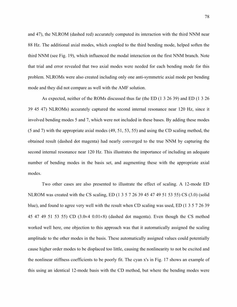
78

and 47), the NLROM (dashed red) accurately computed its interaction with the third NNM near

88 Hz. The additional axial modes, which coupled to the third bending mode, helped soften the

third NNM (see Fig. 19), which influenced the modal interaction on the first NNM branch. Note

that trial and error revealed that two axial modes were needed for each bending mode for this

problem. NLROMs were also created including only one anti-symmetric axial mode per bending

mode and they did not compare as well with the AMF solution.

As expected, neither of the ROMs discussed thus far (the ED (1 3 26 39) and ED (1 3 26

39 45 47) NLROMs) accurately captured the second internal resonance near 120 Hz, since it

involved bending modes 5 and 7, which were not included in these bases. By adding these modes

(5 and 7) with the appropriate axial modes (49, 51, 53, 55) and using the CD scaling method, the

obtained result (dashed dot magenta) had nearly converged to the true NNM by capturing the

second internal resonance near 120 Hz. This illustrates the importance of including an adequate

number of bending modes in the basis set, and augmenting these with the appropriate axial

modes.

Two other cases are also presented to illustrate the effect of scaling. A 12-mode ED

NLROM was created with the CS scaling, ED (1 3 5 7 26 39 45 47 49 51 53 55) CS (3.0) (solid

blue), and found to agree very well with the result when CD scaling was used, ED (1 3 5 7 26 39

45 47 49 51 53 55) CD (3.04 0.018) (dashed dot magenta). Even though the CS method

worked well here, one objection to this approach was that it automatically assigned the scaling

amplitude to the other modes in the basis. These automatically assigned values could potentially

cause higher order modes to be displaced too little, causing the nonlinearity to not be excited and

the nonlinear stiffness coefficients to be poorly fit. The cyan x's in Fig. 17 shows an example of

this using an identical 12-mode basis with the CD method, but where the bending modes were

79

displaced 1.0 times the beam thickness rather than three times. This NLROM did not accurately

represent the backbone of NNM 1, nor the internal resonances. It appears that the bending modes

were not displaced enough in this case to adequately excite the nonlinearity, and as a result the

NLROM coefficients were not accurately estimated. This shows that the scaling for the static

displacements must be carefully selected in order to generate an accurate NLROM.

Next, the convergence of the ICE method was evaluated as bending modes were added to

the basis set using the CLD scaling method for the static loads to fit the nonlinear stiffness

coefficients. The FEPs of NNM 1 in Fig. 18 were computed from NLROMs with modes 1, 3,

modes 1, 3, 5, 7 and modes 1, 3, 5, 7, 9, 11. (Recall that the axial modes do not need to be

included in the basis set when using the ICE method.) Each bending mode used a CLD factor of

0.5 times the thickness, except for mode 11 which used a value of 0.1 time the thickness. These

values were selected in order to keep the nonlinear to linear displacement ratio r near 0.9.

80

10-7

10-6

10-5

10-4

10-3

10-2

10-1

70

80

90

100

110

120

130

Energy, N-m

Fre

quen

cy,

Hz

AMF

ICE (1 3) CLD (0.5 x2) RF (1)

ICE (1 3 5 7) CLD (0.5 x4) RF (1)

ICE (1 3 5 7 9 11) CLD (0.5 x5 0.1) RF (1)

ICE (1 3 5 7 9 11) CLD (0.5 x6) RF (0)

Figure 18. Frequency-energy plot of NNM 1 of the clamped-clamped beam model with ICE

NLROM strategy using higher frequency bending modes.

The NNMs for the ICE method with CLD scaling revealed that NNM 1 converged

quickly along the main backbone, and the two-mode NLROM (short dashed green) captured the

first internal resonance near 88 Hz as soon as the third bending mode was added. The first NNM

converged on the second internal resonance near 120 Hz as modes 5 and 7 were added to the

basis. Overall, the NLROMs agreed with the AMF solution of NNM 1 when the ICE model used

CLD scaling factors and the RF method was used to keep the loads small when forces were

applied in the shape of several modes simultaneously (e.g. RF (1) in the legend means that this

feature was used).

The 6-mode NLROM with the RF method (dashed dot magenta) produced an NNM that

agreed very well with the AMF results, even along the second internal resonance. The ICE

81

method showed considerable sensitivity to the scaling amplitudes when not using the reduction

factor, RF (0), as illustrated by the last line in Fig. 18. This model used a 6-mode basis (modes 1,

3, 5, 7, 9, 11) with a CLD factor of 0.5 times the thickness for mode 11 and no reduction factor

(blue squares). Experience has shown that the RF was more robust and produced more consistent

results as the NNMs seemed to be less sensitive to amplitude of the scale factors.

The next two higher frequency NNMs were computed with the ICE and ED NLROMs

and compared to the results with the AMF algorithm, and are shown in Fig. 19. Each NLROM

was capable of computing the NNM, which is an extension of the linear mode at low energy, as

long as that mode was included in the basis set. NNMs 3 and 5 computed with the two NLROMs

in Fig. 19 agree very well with the AMF solution along the backbone, in fact they practically

overlay each other in the FEP. A small discrepancy existed between the ED NLROM (dashed

red) and AMF (black circles) at the internal resonance near 680 Hz in NNM 3. This was a 5:1

modal interaction with the NNM 9, and since the ED NLROM did not include the ninth bending

mode it was unable to capture this internal resonance (otherwise the two ROMs gave almost

indistinguishable results).

82

10-5

100

400

450

500

550

600

650

700

Energy, N-m

Fre

que

ncy,

Hz

10-5

100

1000

1050

1100

1150

1200

1250

1300

1350

1400

1450

1500

Energy, N-m

(a) (b)

Figure 19. Frequency-energy plot of (a) NNM 3 and (b) NNM 5 of the clamped-clamped beam

model with (black circles) the AMF algorithm, (short dashed green) ICE (1 3 5 7 9 11) CLD (0.5 ×5 0.1) RF (1) and (dashed red) ED (1 3 5 7 26 39 45 47 49 51 53 55) CD (3.0 ×4 0.01 ×8).

4.3 Application to Exhaust Cover Panel with Geometric Nonlinearity

The NLROMs were used to compute the first NNM of a larger, more realistic FEA model

of an exhaust cover plate that exhibited geometric nonlinearity during laboratory tests. The

model reduction strategy becomes even more appealing for this system since it has many more

degrees of freedom than the beam studied in Section 4.2. The mesh for this model is shown in

Fig. 20. The plate was 12.5 inches (318 mm) in diameter, and was constructed of structural steel

with a mass density of 7.29·10-4 lb-s2/in4 (7,800 kg/m3) and a Young's modulus of 30,160 ksi

(208 GPa). The plate was modeled in Abaqus® with 899 S8R shell elements, with a uniform

thickness of 0.0059 inches (1.5 mm), resulting in a total of 15,708 DOF. Each DOF along the

bottom ring of the plate was fixed in all translations and rotations, modeling the relatively rigid

boundary to which the plate was welded.

83

Figure 20. Finite element model of a geometrically nonlinear exhaust cover plate.

A static force was applied to the FEA model that would have displaced the first linear

mode to a maximum displacement of 0.059 inches (1.5 mm), or 1 times the plate thickness. The

computed deformation revealed static coupling to higher frequency modes, which are shown in

Table 4 in descending order of relative modal amplitude. The first five of these linear mode

shapes are plotted in Fig. 21, and serve as candidate modes to successively include in the

NLROM basis. Note that no purely axial or membrane modes appeared to be coupled to the first

bending mode, although mode 156 is predominantly axial. Similar studies of curved beams and

curved panels have shown that axial modes often cease to be distinct from the bending modes

when there is curvature in the structure [114-116].

Table 4. Relative modal amplitude due to a static force applied to excite the first linear mode of the exhaust plate, and the corresponding linear natural frequency.

Mode # 1 6 156 15 30 175 51 74 Amp 1.00 6.8·10-3 4.0·10-3 2.4·10-3 1.5·10-3 1.5·10-3 9.5·10-4 5.6·10-4

Frequency, Hz

156.4 607.5 10,770 1,358 2,402 11,650 3,731 5,328

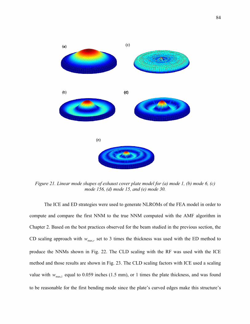
84

Figure 21. Linear mode shapes of exhaust cover plate model for (a) mode 1, (b) mode 6, (c)

mode 156, (d) mode 15, and (e) mode 30.

The ICE and ED strategies were used to generate NLROMs of the FEA model in order to

compute and compare the first NNM to the true NNM computed with the AMF algorithm in

Chapter 2. Based on the best practices observed for the beam studied in the previous section, the

CD scaling approach with rwmax, set to 3 times the thickness was used with the ED method to

produce the NNMs shown in Fig. 22. The CLD scaling with the RF was used with the ICE

method and those results are shown in Fig. 23. The CLD scaling factors with ICE used a scaling

value with 1max,w equal to 0.059 inches (1.5 mm), or 1 times the plate thickness, and was found

to be reasonable for the first bending mode since the plate’s curved edges make this structure’s

85

boundary more compliant than the clamped beam’s. Higher frequency modes used a lower

fraction of the thickness in order to keep the nonlinear to linear displacement ratio r near 0.9.

10-4

10-3

10-2

10-1

100

101

150

155

160

165

170

175

180

185

190

195

200

Energy, N-m

Fre

quen

cy,

Hz

AMF

ED (1) CD (3.0)

ED (1 6) CD (3.0 x2)

ED (1 6 156) CD (3.0 x3)

ED (1 6 15 30 51 74 156 175) CD (3.0 x8)

Figure 22. Frequency-energy plot of NNM 1 of the exhaust cover plate model with ED NLROM

strategy using higher frequency bending modes.

The ED method did not perform as well for this system as it did for the beam. A single-

mode NLROM was greatly in error, yet results for the first NNM improved somewhat as

additional modes were added to the ED basis. Even after including the eight modes that were

most strongly coupled to the first bending mode, as shown in Table 4, the FEP was off by nearly

an order of magnitude in energy at 190 Hz. The FEA model of the clamped-clamped beam

showed that including axial type modes greatly improved the accuracy of the ED NLROM.

However, no pure membrane modes existed for the exhaust cover plate due to its slight

curvature, so this remedy was not available.

86

10-4

10-3

10-2

10-1

100

101

150

155

160

165

170

175

180

185

190

195

200

Energy, N-m

Fre

quen

cy,

Hz

AMF

ICE (1) CLD (1.0) RF (1)

ICE (1 6) CLD (1.0 0.25) RF (1)

ICE (1 6 156) CLD (1.0 0.25 0.01) RF (1)

ICE (1 6 15 30) CLD (1.0 0.25 x3) RF (1)

Figure 23. Frequency-energy plot of NNM 1 of the exhaust cover plate model with ICE NLROM

strategy using higher frequency bending modes.

The NNM estimated by a one-mode NLROM (short dashed green) constructed using the

ICE method was only slightly in error at higher energies, and the NLROM quickly converged to

the true NNM when mode 6 was added to the basis (dashed red). The sixth bending mode had a

strong coupling to the first NNM, and hence it is not surprising that this mode had an important

dynamic effect. Using this NLROM, the first NNM could be computed much more efficiently

than the AMF algorithm on the full order model; only about 15 minutes were needed to solve the

nonlinear static load cases to create the two-mode NLROM and compute the first NNM branch.

In contrast, running the AMF algorithm on the full model took approximately 4 days.

Two other cases are also shown in Fig. 23 to illustrate a potential pitfall of the ICE

strategy. When the next dominant mode, mode 156, was added to the ICE basis set (blue

87

squares), the first NNM diverged. The FEA model had difficulty converging in the static load

cases used to create the NLROM with mode 156. By using a small enough CLD factor with

156max,w equal to 0.01 times the plate thickness, the static results finally converged resulting in a

nonlinear to linear ratio of 156 = 0.98. It was decided that mode 156 should be removed from the

basis set, and the next two modes (15 and 30) included instead, producing the result shown with

the dashed dot magenta line. The resulting four-mode NLROM again predicted the first NNM

very accurately. This example highlights the importance of mode selection with the reduced

order modeling strategy. The fact that mode 156 had a much higher frequency leads one to

believe that this mode only needs to be included implicitly, and should not be included explicitly

in the basis set. Based on these results, the ICE method seemed to be better suited for systems

with many DOF, as long as the modes are scaled appropriately and the correct modes are added

to the basis.

4.4 Simply Supported Beam with Contacting Nonlinearity

The reduced order models of the beam in Fig. 24 are generated using a Galerkin approach

with linear vibrations modes augmented with discontinuous basis functions, as done in [40, 113].

The linear, simply supported beam is modeled in Abaqus® using 40 B31 beam elements,

resulting in a total of 119 DOF. The contact is modeled as a linear spring with a unilateral

piecewise-linear function at a distance l1 from the left support, with a spring stiffness of k and

clearance a. When the spring is engaged, it applies a force on the beam in the transverse

direction, resulting in a non-smooth, nonlinear system of equations. The spring in this example is

located at the midpoint of the beam with l1 = 4.5 inches (114 mm) and a clearance of a = 0.0155

88

inches (0.394 mm). The material and geometric properties of the beam in Fig. 24 are given in

Table 5.

a

L

l1

k

a

L

l1

k

Figure 24. Schematic of simply supported beam with discrete contact nonlinearity.

Table 5. Material and geometric properties of the nonlinear beam model.

Property Value Young's Modulus 29,700 ksi (204.8 GPa) Poisson's Ratio 0.28 Shear Modulus 11,600 ksi (80.0 GPa)

Density 7.36·10-4 lb-s2/in4 (7,870 kg/m3)

Length 9 inches (229 mm) Width 0.5 inches (12.7 mm) Thickness 0.031 inches (0.787 mm) Keq 9.7 lbf/inch (1.70 kN/m) … … Spring Stiffness, k 200 lbf/inch (35.0 kN/m) Spring Clearance, a 0.0155 inches (0.394 mm) Spring Location, l1 4.5 inches (114 mm)

Prior to the nonlinear modal convergence analysis, the first seven linear modes of the

beam were computed, and the corresponding natural frequencies are listed in Table 6. Each is a

low frequency bending mode, where the even mode numbers are asymmetric shapes and the odd

numbers are symmetric. Only the odd bending modes are used in the reduction scheme, since all

of the even modes have nodal points at the impact location. Since the nonlinearity is localized to

only a single DOF, only a single discontinuous basis vector was computed for each ROM, and

89

was orthonormalized with respect to the mass matrix. As a result, this augmented basis vector

changed depending on which linear modes were included in the basis set.

Table 6. Linear natural frequencies of simply supported beam.

Mode 1 Mode 2 Mode 3 Mode 4 Mode 5 Mode 6 Mode 7 34.8 Hz 139.4 Hz 313.8 Hz 558.2 Hz 872.7 Hz 1258 Hz 1714 Hz

The NNMs from various ROMs are computed to study the convergence of the beam as

modes are added to the basis set. In this study, ROMs with mode (1), modes (1 MC), modes (1 3

5 MC) and modes (1 3 5 7 9 11 MC) were generated using the approach described in [113]. The

Milman-Chu (MC) mode is the added discontinuous basis vector used to improve the kinematic

constraints at the location of the contacting spring, while the others are the mode numbers of the

linear bending mode shapes computed from the linear mass and stiffness matrix. The first, third

and fifth NNMs (all symmetric) were computed from these ROMs, and the resulting frequency-

energy plots are presented in Figs. 25 to 28.

90

10-6

10-4

10-2

100

102

35

40

45

50

55

60

65

Energy, in-lbf

Fre

quen

cy,

Hz

ROM [1]

ROM [1 MC]ROM [1 3 5 MC]

ROM [1 3 5 7 9 11 MC]

(B)

(A)

Figure 25. The first NNM computed for the (dotted magenta) ROM with mode (1), (dashed

green) ROM with modes (1 MC), (dash-dot red) ROM with modes (1 3 5 MC), and (short dashed blue) ROM with modes (1 3 5 7 9 11 MC). Time response of solutions (A) and (B) are plotted in

Fig. 26.

The first NNM was initiated at the first linear mode with a frequency of 34.8 Hz, and was

computed out to a 69% shift in fundamental frequency (with the 7-mode ROM). At low energy,

the response amplitude was low enough that the contacting spring did not engage with the beam,

and the periodic response was exactly that of the first linear bending mode. The linear response

range is seen by the straight line in the frequency-energy plane in Fig. 25 below 3.0·10-4 in-lbf.

Once the midpoint amplitude of the first bending mode reached the spring clearance (a = 0.0155

inches), the engaged spring caused the NNM to change. The transition from linear to nonlinear

occurred at an energy of 3.0·10-4 in-lbf, and the periodic responses stiffened (i.e. increased in

frequency) due to the added stiffness of the contact.

91

Two features of the NNM branch are observed in this nonlinear range: the backbone and

the modal interactions that emanate from the backbone (e.g. the sharp peaks with nearly constant

frequency in the FEP). These deviations from the backbone occur when two or more modes

interact, and exchange energy with other NNMs of the ROM. The plots in Fig. 26 show the time

response of the two points marked (A) and (B) in Fig. 25 from the ROM with modes (1 3 5 7 9

11 MC). The response of solution (A) oscillates with a frequency of about 41.2 Hz

predominantly in the shape of the first bending mode. Through one period of response, Figs. 26a

and 26b show that this NNM solution contains higher order harmonics as well as contributions of

higher order bending modes. Solution (B) reveals the periodic motion along one of its (many)

internal resonances occurring at a frequency of about 50.4 Hz. This was a 34:1 interaction with

the 7th mode, meaning that NNM 7 oscillated at a frequency 34 times the frequency of the first

NNM. The deformation shapes in Fig. 26c show the complicated response through different

snapshots of time with strong contributions from the 1st and 7th mode shapes.

92

0 2 4 6 8-0.02

-0.01

0

0.01

0.02

Location, inch

Dis

plac

emen

t, in

ch

Increasing Time

0 2 4 6 8-0.05

-0.04

-0.03

-0.02

-0.01

0

0.01

0.02

Location, inch

Dis

plac

emen

t, in

ch

Increasing Time

0 0.005 0.01 0.015 0.02 0.025-0.02

-0.01

0

0.01

0.02

Time, s

Dis

plac

emen

t, in

ch

0 0.005 0.01 0.015 0.02-0.06

-0.04

-0.02

0

0.02

Time, s

Dis

plac

emen

t, in

ch

Solution (A) Solution (B)

(a)

(b)

(c)

(d)

Figure 26. Time history of NNM solutions (A) and (B) in Fig. 25 for the ROM with modes (1 3 5 7 9 11 MC). Plots (a) and (c) show the beam deflection shape at different snapshots in time, and

plots (b) and (d) show the time history of the contacting DOF over one period.

The first NNM in Fig. 25 from the ROM with mode (1) captured the linear solution at

energies below 3.0·10-4 in-lbf, but did not accurately capture the backbone in the nonlinear range.

For example, at an energy level of 5.0 in-lbf, this ROM predicted a frequency of 62.5 Hz,

whereas the other ROMs predicted 58.7 Hz (an error of 6.5%). The (1 MC) ROM captured the

backbone quite accurately, revealing that the MC mode greatly improved the accuracy of the

ROM. On the other hand, the ROM with modes (1 MC) only computed 3 internal resonances,

which was significantly fewer than the amount captured with the higher fidelity ROMs. The

contacting spring was coupling higher order modes into the response, so several additional

modes were needed in the basis set to accurately capture these internal resonances. The backbone

93

appears to be converged to high precision with the (1 3 5 MC) and (1 3 5 7 9 11 MC) mode

ROMs. However, the internal resonances of these ROMs have not yet converged, as the 7-mode

ROM still introduced many new tongues along the backbone and few, if any, agree with those of

the 4-mode ROM. This comparison revealed that a relatively simple ROM can accurately capture

the backbone of NNM 1, but tremendously more effort would be needed if internal resonances

were to also converge.

10-4

10-3

10-2

10-1

100

101

102

313

313.5

314

314.5

315

315.5

316

316.5

317

317.5

318

Energy, in-lbf

Fre

quen

cy,

Hz

ROM [3]

ROM [3 MC]

ROM [1 3 5 MC]

ROM [1 3 5 7 9 11 MC]

Figure 27. The third NNM computed for the (dotted magenta) ROM with mode (1), (dashed

green) ROM with modes (1 MC), (dash-dot red) ROM with modes (1 3 5 MC), and (short dashed blue) ROM with modes (1 3 5 7 9 11 MC).

The FEP of the third NNM is plotted in Fig. 27 for ROMs generated with mode (3),

modes (3 MC), modes (1 3 5 MC), and modes (1 3 5 7 9 11 MC). The third NNM has the same

features as the first NNM in Fig. 25, but is much simpler since only one internal resonance

appears at 315.8 Hz. The nonlinear region of the third NNM started at an energy of 2.4·10-4 in-

lbf, and below this level the beam oscillated in exactly the third bending mode with a frequency

94

of 313.8 Hz. Above 2.4·10-4 in-lbf, the spring was engaged and caused the fundamental

frequency of the motion to increase. The third NNM had a frequency shift of about 1.0 %, which

was significantly less than that of the first NNM. Again, the ROM computed with mode (3) did

not accurately capture the backbone, and the one-mode model was far too stiff. The accuracy of

this ROM improved greatly when one discontinuous basis vector was added to the basis,

however additional bending modes did not significantly change the backbone. As the model

order increased, there was an internal resonance that occurred at 315.8 Hz, which was only

computed with the ROM with modes (1 3 5 7 9 11 MC). It was discovered that this internal

resonance was a 9:1 interaction with the 9th NNM of the beam, and hence could not be captured

unless the kinematics of the 9th bending mode were included in the basis. Other internal

resonances may also be captured with additional bending modes, but this was not pursued

further.

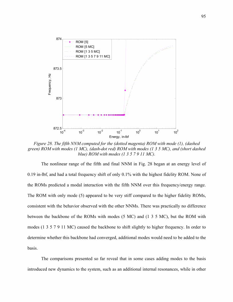
95

10-4

10-3

10-2

10-1

100

101

102

872.5

873

873.5

874

Energy, in-lbf

Fre

quen

cy,

Hz

ROM [5]

ROM [5 MC]

ROM [1 3 5 MC]

ROM [1 3 5 7 9 11 MC]

Figure 28. The fifth NNM computed for the (dotted magenta) ROM with mode (1), (dashed

green) ROM with modes (1 MC), (dash-dot red) ROM with modes (1 3 5 MC), and (short dashed blue) ROM with modes (1 3 5 7 9 11 MC).

The nonlinear range of the fifth and final NNM in Fig. 28 began at an energy level of

0.19 in-lbf, and had a total frequency shift of only 0.1% with the highest fidelity ROM. None of

the ROMs predicted a modal interaction with the fifth NNM over this frequency/energy range.

The ROM with only mode (5) appeared to be very stiff compared to the higher fidelity ROMs,

consistent with the behavior observed with the other NNMs. There was practically no difference

between the backbone of the ROMs with modes (5 MC) and (1 3 5 MC), but the ROM with

modes (1 3 5 7 9 11 MC) caused the backbone to shift slightly to higher frequency. In order to

determine whether this backbone had converged, additional modes would need to be added to the

basis.

The comparisons presented so far reveal that in some cases adding modes to the basis

introduced new dynamics to the system, such as an additional internal resonances, while in other

96

cases they simply improved the accuracy of the backbone (e.g. when the model was augmented

from (1) to (1 MC)). In the results shown here, the backbones of the first and third NNM appear

to converge with the 7-mode ROM, but the internal resonances have not yet converged. Due to

the complexity of the internal resonances, and the potentially infinite number of these solutions,

the question remains: how important are these to the accuracy of the ROMs for other predictive

purposes (e.g. solutions to a forced response)? Do these internal resonances manifest themselves

in the response?

This question was addressed to a certain extent in a paper by Ardeh & Allen [42] where

the response of a 2DOF nonlinear system was studied in detail, revealing that many other NNM

branches exist with much lower fundamental frequencies than those extending from the linear

modes. These solutions form manifolds in the state space that are tangent to the fundamental

NNM manifolds, hence a response on one manifold can easily travel onto (or along) another.

This, and the erratic convergence of the first NNM presented above, suggests that the transient

response of this system may be quite difficult to predict with great precision. In the following

subsection the transient response is presented for a few different load amplitudes in order to

explore the correlation between the accuracy of the transient response computed by each ROM

and their convergence of the underlying NNMs.

4.4.1 Impulse Loading Validation

The first load considered was an impulsive load modeled by a half-sine pulse in time.

Spatially, the impulse was given the shape of the first linear bending mode, such that

tgAt 1Mφf , where g(t) is a half-sine pulse over a short time duration with a prescribed

amplitude A. This load was chosen to excite the beam near its first NNM branch, where the

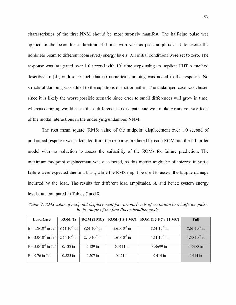
97

characteristics of the first NNM should be most strongly manifest. The half-sine pulse was

applied to the beam for a duration of 1 ms, with various peak amplitudes A to excite the

nonlinear beam to different (conserved) energy levels. All initial conditions were set to zero. The

response was integrated over 1.0 second with 107 time steps using an implicit HHT method

described in [4], with =0 such that no numerical damping was added to the response. No

structural damping was added to the equations of motion either. The undamped case was chosen

since it is likely the worst possible scenario since error to small differences will grow in time,

whereas damping would cause these differences to dissipate, and would likely remove the effects

of the modal interactions in the underlying undamped NNM.

The root mean square (RMS) value of the midpoint displacement over 1.0 second of

undamped response was calculated from the response predicted by each ROM and the full order

model with no reduction to assess the suitability of the ROMs for failure prediction. The

maximum midpoint displacement was also noted, as this metric might be of interest if brittle

failure were expected due to a blast, while the RMS might be used to assess the fatigue damage

incurred by the load. The results for different load amplitudes, A, and hence system energy

levels, are compared in Tables 7 and 8.

Table 7. RMS value of midpoint displacement for various levels of excitation to a half-sine pulse in the shape of the first linear bending mode.

Load Case ROM (1) ROM (1 MC) ROM (1 3 5 MC) ROM (1 3 5 7 9 11 MC) Full

E = 1.8·10-4 in-lbf 8.61·10-3 in 8.61·10-3 in 8.61·10-3 in 8.61·10-3 in 8.61·10-3 in

E = 2.0·10-3 in-lbf 2.54·10-2 in 2.49·10-2 in 1.61·10-2 in 1.51·10-2 in 1.50·10-2 in

E = 5.0·10-2 in-lbf 0.133 in 0.129 in 0.0711 in 0.0699 in 0.0688 in

E = 0.76 in-lbf 0.525 in 0.507 in 0.421 in 0.414 in 0.414 in

98

Table 8. Maximum value of midpoint displacement for various levels of excitation to a half-sine pulse in the shape of the first linear bending mode.

Load Case ROM (1) ROM (1 MC) ROM (1 3 5 MC) ROM (1 3 5 7 9 11 MC) Full

E = 1.8·10-4 in-lbf 1.21·10-2 in 1.21·10-2 in 1.21·10-2 in 1.21·10-2 in 1.21·10-2 in

E = 2.0·10-3 in-lbf 4.05·10-2 in 4.05·10-2 in 3.84·10-2 in 3.92·10-2 in 3.92·10-2 in

E = 5.0·10-2 in-lbf 2.03·10-1 in 2.04·10-1 in 1.94·10-1 in 1.88·10-1 in 1.85·10-1 in

E = 0.76 in-lbf 0.786 in 0.792 in 0.778 in 0.762 in 0.762 in

For the predicted response at low energy (E = 1.8·10-4 in-lbf), the maximum displacement

in Table 8 for each model was 0.0121 inches, which was below the contact clearance of a =

0.0155 inches. The beam responded exactly in the first linear mode, and all of the models were in

perfect agreement. Knowing the system energy of the response, the frequency-energy plot of the

first NNM in Fig. 25 reveals that the system energy is in the linear range. However, the higher

energy load cases in Tables 7 and 8 show that the energy of each response are in the nonlinear

range of the first NNM. The ROMs with mode (1) and modes (1 MC) do not accurately predict

the RMS and maximum displacements of the full order model at the higher energy levels. When

looking at the first NNM, the nonlinear modal convergence analysis of each of these ROMs

determined that additional modes were needed in the basis to capture the modal interactions

predicted by the higher order ROMs. The mode (1) ROM showed considerable error in the

backbone while the (1 MC) ROM captured it reasonably well. This confirms that the internal

resonances do play an important role in the transient response, at least in the undamped case.

It is interesting to note that the 4-mode and 7-mode ROMs predict the RMS and

maximum displacements quite accurately for each load case. In fact, the ROM with modes (1 3 5

99

7 9 11 MC) agrees very well with the full order model in the nonlinear range, with the largest

error occurring when the system energy level was E = 5.0·10-2 in-lbf and the ROM overpredicted

the RMS displacement by 1.5%, and the maximum displacement by 1.6%. This ROM was quite

acceptable even though it could not be confirmed that its first NNM had converged at all of the

system’s internal resonances. The internal resonances represent manifolds in the state space that

connect different nonlinear modes; perhaps the ROMs need only capture the location (in terms of

frequency and energy) and the density of these interactions in order to allow energy to propagate

correctly and hence to predict the RMS and maximum displacement accurately.

The first 0.5 seconds of the displacement at the center of the beam is plotted in Fig. 29 for

the full order model, and two of the ROMs (low and high fidelity), both of which include the

augmented discontinuous basis vector. The ROM with modes (1 MC) (green dashed)

overpredicts the amplitude of the response for all load cases in the nonlinear region (Fig. 29b-

29d), and appears to be dominated by a single frequency.

100

0 0.1 0.2 0.3 0.4 0.5-0.015

-0.01

-0.005

0

0.005

0.01

0.015

Time, s

Dis

plac

emen

t, in

ch

Full

ROM [1 MC]

ROM [1 3 5 7 9 11 MC]

0 0.1 0.2 0.3 0.4 0.5-0.05

-0.04

-0.03

-0.02

-0.01

0

0.01

0.02

Time, s

Dis

plac

emen

t, in

ch

0 0.1 0.2 0.3 0.4 0.5-0.25

-0.2

-0.15

-0.1

-0.05

0

0.05

0.1

Time, s

Dis

plac

emen

t, in

ch

(a) (b)

(c)

0 0.1 0.2 0.3 0.4 0.5-0.8

-0.6

-0.4

-0.2

0

Time, s

Dis

plac

emen

t, in

ch

(d)

0 0.1 0.2 0.3 0.4 0.5-0.015

-0.01

-0.005

0

0.005

0.01

0.015

Time, s

Dis

plac

emen

t, in

ch

Full

ROM [1 MC]

ROM [1 3 5 7 9 11 MC]

0 0.1 0.2 0.3 0.4 0.5-0.05

-0.04

-0.03

-0.02

-0.01

0

0.01

0.02

Time, s

Dis

plac

emen

t, in

ch

0 0.1 0.2 0.3 0.4 0.5-0.25

-0.2

-0.15

-0.1

-0.05

0

0.05

0.1

Time, s

Dis

plac

emen

t, in

ch

(a) (b)

(c)

0 0.1 0.2 0.3 0.4 0.5-0.8

-0.6

-0.4

-0.2

0

Time, s

Dis

plac

emen

t, in

ch

(d)

Figure 29. Response of contacting DOF due to a half-sine pulse in the shape of the first linear

mode with system energy of (a) E = 1.8·10-4 in-lbf, (b) E = 2.0·10-3 in-lbf, (c) E = 5.0·10-2 in-lbf, and (d) E = 0.76 in-lbf. (Solid black) full order model, (dashed green) ROM with modes (1 MC),

and (short dashed blue) ROM with modes (1 3 5 7 9 11 MC).

In contrast, the ROM with modes (1 3 5 7 9 11 MC) closely follows the response

predicted by the full model, capturing the higher harmonics and the relative amplitude of the

displacement, although the predicted response does have a significant phase error after about 0.3

seconds. This divergence is common for systems with non-smooth nonlinearities. The first NNM

in Fig. 25 shows many internal resonances at E = 2.0·10-3 in-lbf, suggesting that the beam's

response at this energy level could travel along one of these manifolds and pump energy into

another nonlinear mode of the system, as was observed in the transient responses in [42]. Since

101

the 7-mode ROM did not appear to converge at all of the internal resonances, the response that it

predicts may travel along other nearby paths potentially transferring energy to different nonlinear

modes and ultimately causing the time response to diverge.

It is interesting to point out that Figure 29d shows that at E = 0.76 in-lbf , the signals

between the full model (solid black) and the ROM with modes (1 3 5 7 9 11 MC) (blue dotted)

stay in phase over the entire period and appear to be in very good agreement. Figure 25 shows

that, at this energy level, the backbone of the first NNM has leveled off and there are fewer

internal resonances that can come into the path of the system; perhaps this causes the response to

be more likely to travel on the manifold described by NNM 1 backbone and to oscillate at a fixed

frequency. Even the (1 MC) ROM does a sufficient job at predicting the maximum and (to a

lesser extent) RMS amplitudes and the frequency content in the response, further reinforcing the

idea that the backbone is more important than the internal resonances at this energy level.

These comparisons have shown that, although the response of this beam shows vastly

different character at different energy levels, its response is somehow connected to its nonlinear

normal modes. A reduced order model that captures its nonlinear modes accurately is likely to

correctly predict its response over the corresponding range of energy. In the next subsection, the

damped ROMs are compared to the full order model using a random force input to evaluate the

response capabilities with structural damping.

4.4.2 Random Loading Validation

The response to a random force applied at the midpoint of the beam in the transverse

direction is presented here. A linear damping model was included in the reduced and full order

equations of motion based on mass and stiffness proportional damping (i.e. KMC ), with

102

and chosen so that the first and third modes of the linear beam had modal damping ratios of

0.5 %. The linear, diagonal damping matrix for the ROMs was derived from this diagonalizable

damping matrix, C . The lightly damped beam was forced using a broadband, Gaussian random

input with zero mean and a standard deviation of . The input was filtered using an 8th order

Butterworth filter with a cutoff frequency of 1,000 Hz, in order to excite (at least) the first three

symmetric modes of the system. Figure 30 shows the autospectrum of the midpoint displacement

for a forcing level with a standard deviation of = 0.1 lbf.

0 50 100 150 200 250 300 350 400 450 500

10-10

10-5

Frequency, Hz

Ce

nte

r D

isp

lace

me

nt S

pe

ctra

l De

nsi

ty, i

n2/H

z

FullROM [1]ROM [1 MC]ROM [1 3 5 MC]ROM [1 3 5 7 9 11 MC]

Figure 30. Autospectrum of the midpoint transverse displacement to a random force input with a

standard deviation of = 0.1 lbf.

All of the models show that the response was dominated by a peak around 54 Hz, which

can be attributed to the first NNM. The harmonics of this peak occur at 108.8 Hz, 168 Hz, and so

forth, and were especially prominent in the response of the one-mode ROM. Since this one-mode

ROM did not have any internal resonances along the first NNM, these harmonics come from the

response of the first mode. Some of those harmonics were visible in the response of the higher

order ROMs. Overall the one-mode ROM poorly predicted the frequencies and amplitudes of

these peaks. Furthermore, while this ROM predicted that the dominant frequency was near 54

103

Hz, the model was stiffer than the full order model since it overpredicted the response near the

first mode, presumably because it did not have the pathways that would allow vibration energy to

transfer to other NNMs.

The response predicted by the (1 MC) model improved near the 54 Hz resonance peak (as

expected based on its NNM backbone), but it still overpredicted the amplitude of the response by

a significant amount. It appeared that the first mode exchanged energy with the third mode and

hence the model must explicitly include that mode in the basis in order to predict the response

level accurately. The higher fidelity ROMs with modes (1 3 5 MC) and (1 3 5 7 9 11 MC) agree

very well with the results from the full order model. The autospectrum in Fig. 30 suggests that

the convergence of the backbone is the most important feature of the modal convergence study to

infer about the accuracy of the damped response to a random load since the 4-mode and 7-mode

ROMs predicted nearly the same response as the full order model, but predicted different internal

resonances. The internal resonances are known to be important to some degree, however, since

one could create a 7-mode model that neglects the coupling between the modes, and while such a

model might capture accurately the backbones it would not predict the response amplitudes very

accurately. This was illustrated in [41]. Even then, it appeared that for a system like this it was

not critical that each internal resonance converge, as long as the system has some internal

resonances at the energy level of interest.

4.5 Summary

This chapter presented three case studies involving reduced order models of nonlinear

FEA models. The accuracy of these were evaluated based on the computed nonlinear normal

modes either as modes were added to the basis, or as the scaling on the static loads were

adjusted. The ICE and ED reduced order modeling strategies were used in Sections 4.2 and 4.3

104

to reduce two geometrically nonlinear finite element models to a low order set of nonlinear

modal equations. The NNMs of the clamped-clamped beam and an exhaust cover plate helped

guide the decisions to generate accurate models and were invaluable in this regard. NNMs are

relatively inexpensive to compute from the NLROM and they readily show the differences and

similarities between a candidate set of NLROMs and give physical insight into how the

responses of the NLROMs might differ.

One disadvantage of the ED method is the requirement to include axial modes in the

basis set, causing these ROM to have more DOF than those created with ICE. This increases the

size of the NLROM, although it is still dramatically smaller than the original finite element

model. Fortunately, the results have shown that a simple static force in the shape of a particular

vibration mode can reveal which modes are coupled to it and should be augmented to the ED

NLROM basis. The ICE NLROMs converged quickly for each finite element model studied in

Chapter 4, requiring only a few modes to at least capture the NNM backbones. The ED method

converged for the geometrically nonlinear beam with relatively few modes, but did not converge

for the exhaust cover plate. A recent study [71] suggests that using dual modes [67] to capture

the membrane kinematics improves the ED basis. The results on the exhaust cover plate in that

paper converged to the backbone with only two bending modes and three dual modes.

The third case study presented here demonstrated the NNM convergence metric on a

simply supported beam with a non-smooth, contact nonlinearity. The first NNM of the beam

appeared to have converged along the backbone with either a four or seven mode ROM, however

the internal resonance were not yet converged. The difficulty in computing the tongues along

with the high density of these solutions made it difficult to evaluate the convergence of the

system without studying higher order ROMs. The ROMs were validated with the full order

105

model by comparing the responses to an impulsive load and a random external force. The

convergence along the backbone suggests that the peak and RMS response to an impulsive force

will be in agreement, however the internal resonances seem to contribute to the divergence of the

two signals over time. These results suggest that a ROM that accurately captured the backbone

(and also included a similar density of internal resonances) would be adequate to predict the

random and transient response, although no formal proof was shown.

It is believed that the comparison of nonlinear normal modes has great promise for other

model reduction strategies of conservative systems. Previous works have focused on comparing

the transient response or the power spectra of the response when a random input is applied, but

those each depend on a forcing function and/or a prescribed initial condition. In contrast, the

NNMs are unique solutions to the undamped equations of motion that exercise the model over a

range of response amplitudes (or energy levels), and they are relatively quick to compute using

numerical continuation algorithms. This work has shown that the NNMs serve as a valuable

metric to assess the convergence of a NLROM equations, even if the reference solutions from the

full order model are not available.

106

5 Nonlinear Modal Substructuring

5.1 Introduction

A modal substructuring approach for geometrically nonlinear FEA models is proposed

here by generating subcomponent reduced order models using the Implicit Condensation and

Expansion procedure [19, 103] reduced with either

i.) free-interface modes

ii.) fixed-interface plus constraint modes (Craig-Bampton (CB) modes)

iii.) fixed-interface plus characteristic constraint (CC) modes

After the subcomponent modal models are identified, they are assembled by satisfying force

equilibrium and compatibility, just as done with linear systems [54, 74] or in finite element

assembly [28]. Kuether and Allen first developed this nonlinear modal substructuring approach

for subcomponent ROMs reduced with free-interface modes in [93], and later used fixed-

interface plus constraint modes on the same assembly of two geometrically nonlinear beams

having a connection interface with only 1-DOF [104, 105]. For a continuous interface with more

than a few DOF, the number of static constraint modes would prohibit the use of ICE, or any

ROM approach, hence motivating the use of characteristic constraint modes [82] to reduce the

interface DOF. Kuether and Allen used fixed-interface plus characteristic constraint modes in

[106] and then [107] to reduce the interface DOF of two geometrically nonlinear plate models

with many connection points.

Dynamic substructuring analysis first divides the global structure of interest into smaller

substructures, whose equations are reduced before being assembled to give a reduced order

model. Therefore, the derivation starts with the discretized, geometrically nonlinear finite

107

element model of a subcomponent, giving the undamped, N-degrees-of-freedom equations of

motion in the form,

tNL fxfKxxM )(

(54)

where M and K are the NN linear mass and stiffness matrices, respectively. xf NL is the

1N nonlinear restoring force vector that accounts for the internal forces due to geometric

nonlinearity. The 1N vectors x , x , and tf are the displacement, acceleration and external

forces, respectively. The damping matrix can readily be included as well but will be omitted here

for brevity. The nonlinear modal substructuring procedure is outlined in the following three

subsections. Section 5.2 discusses a few choices for subcomponent modes to reduce each

subcomponent FEA model in Eq. (54), Section 5.3 generates the reduced subcomponent model

based on the modal basis chosen in Section 5.2, and Section 5.4 couples the nonlinear

subcomponent models to obtain a reduced order model of the assembly.

5.2 Component Mode Basis Selection

In order to reduce each subcomponent FEA model, first a set of subcomponent modes, or

Ritz vectors, are needed to capture the kinematics. This chapter presents three different types of

linear basis functions used for substructuring and their theory is reviewed here. There are a

variety of other modal bases that could be used [74] but only those listed below are addressed in

this dissertation.

5.2.1 Free-interface Modes

The free-interface modes (e.g. with no boundary constraints applied to the interface DOF)

are the linear vibration modes computed from the linear mass and stiffness matrices in Eq. (54)

108

and are found by solving the eigenvalue problem rr φMK 2 . The modal transformation

matrix using a truncated set of these mode shapes is given as,

FIFI qTx (55)

The mN matrix, FIT , contains a truncated set of mass normalized, free-interface mode shapes,

rφ , in each of its columns. The reduced coordinate space FIq is significantly smaller than the

physical coordinate space x (i.e. m << N).

5.2.2 Craig-Bampton Modes

Again starting with the linear form of the equations of motion in Eq. (54) (i.e. when

0xf NL ), each DOF in x is first partitioned into either boundary DOF, bx , or interior DOF.

ix . The boundary DOF are either shared by an adjacent structure, sometimes referred to as

interface DOF, or may have been retained simply because an external point load tf is applied

to that location. The interior DOF are all the remaining coordinates of the system. The

partitioned equations of motion of the linear model become

tb

i

bbbi

ibii

b

i

bbbi

ibii

f

0

x

x

KK

KK

x

x

MM

MM

(56)

The fixed-interface modes are computed by restraining all the boundary coordinates, bx ,

and solving the eigenvalue problem 0φMK riiiiriiii ,2, from the linear system matrices

partitioned to only the interior DOF, ix , in Eq. (56). These fixed-interface modes are then mass

normalized with respect to iiM . These mode shapes are augmented with a set of static shapes,

known as constraint modes, that account for deformations at the boundary, or interface, DOF.

109

One constraint mode is computed for every boundary coordinate in bx by computing the static

deflection to a unit displacement at each boundary DOF while holding the other boundary

coordinates fixed. These shapes are computed as

bb

ibii

bb

ib

I

KK

I

ΨΨ

1

(57)

The modal transformation matrix with fixed-interface modes and constraint modes then becomes

CBCBb

kibik

b

i qTx

q

I0

ΨΦ

x

x

(58)

where ikΦ is the ki NN matrix of mass normalized fixed-interface modes, I is the identity

matrix, and Ψ is the bNN matrix of constraint modes. Typically, only a small set of kN

fixed-interface modes are needed in the basis and this truncation determines the level of accuracy

of the assembled ROMs, as seen later in Chapter 6. The total number of modal coordinates in the

vector CBq is the number of retained fixed-interface modes kN plus the number of constraint

modes bN , denoted as bk NNm . The resulting mN matrix CBT is known in the literature

as the Craig-Bampton transformation matrix, as discussed in [74, 76].

5.2.3 Craig-Bampton Modes with Interface Reduction

To initiate the interface reduction using characteristic constraint modes [82], a linear

reduced order model of the subcomponent is created by substituting Eq. (58) into Eq. (56) and

pre-multiplying by the transpose, T , of the CB transformation matrix, TCBT . A linear CB

reduced order model for a subcomponent has the form,

110

ttb

k

bbbk

kbkk

b

k

bbbk

kbkk

rfx

q

K0

0Λ

x

q

MM

MI 0ˆˆˆ

ˆ

(59)

The vector tr is the unknown equal and opposite reaction force that will be applied by an

adjacent connecting structure, and kkΛ is a diagonal matrix of squared natural frequencies of the

fixed-interface modes. For FEA models with a very detailed mesh at the interface, there may be

many thousands of DOF at the boundary requiring far too many constraint modes, Ψ . A

reduction of these boundary coordinates, bx , is sought using the approach in [82] by performing

a second modal analysis. This is done by first assembling all the linear CB models from Eq. (59)

following the classical CB approach [74, 76]. Without loss of generality, coupling two linear

subcomponents denoted with superscripts (A) and (B) produces the equations of motion of the

assembly

)(ˆˆˆˆˆˆ

ˆ

ˆB

A

BA

B

A

B

A

BABA

BB

AA

tb

k

k

bbbb

kk

kk

b

k

k

bbbbbkbk

bkkk

bkkk

B

A

BB

AA

B

A

BA

BBB

AAA

f

0

0

x

q

q

KK00

0Λ0

00Λ

x

q

q

MMMM

MI0

M0I

(60)

A second modal analysis is performed on the linear mass and stiffness matrices

corresponding to the boundary DOF, bx , in Eq. (60) by solving the eigenvalue problem

0ψMMKK rCCbbbbrbbbb ,

BA2BA ˆˆˆˆ (61)

These boundary mode shape vectors, rCC ,ψ , are then truncated and used to assemble the

cb NN matrix CCΨ . The work in [82] uses this transformation to further reduce the assembly

equations of motion in Eq. (60). However, this dissertation is interested in reducing the number

111

of constraint modes used to describe the interface in the CB transformation in Eq. (58), so CCΨ

reduces the interface DOF as,

CCCCc

k

bc

icik

c

k

CC

ibik

b

i qTq

q

Ψ0

ΨΦ

q

q

Ψ0

0I

I0

ΨΦ

x

xx

ˆ

ˆ (62)

Ψ̂ is now the cNN matrix of characteristic constraint modes that capture the "characteristic"

motion of the interface for a single subcomponent due to its connection to other subcomponents.

The total number of generalized coordinates in the vector CCq becomes ck NNm , and the

mN matrix CCT contains the fixed-interface modes and now the characteristic constraint

modes. The generalized coordinates in the 1m vector CCq have significantly fewer DOF than

total number of N physical DOF in Eq. (54), and the number of CB modal coordinates in Eq.

(58).

5.3 Reduced Subcomponent Models with Geometric Nonlinearity

Without loss of generality, the modal basis for a subcomponent model is denoted with the

matrix T and generalized coordinates q without the subscripts, as the following reduction

procedure applies for any of the three modal bases given by Eqs. (55), (58), and (62). In order to

reduce the full order, geometrically nonlinear model in Eq. (54), again the displacements, x , are

sorted to the boundary and interior DOF as,

tbNL

iNL

b

i

bbbi

ibii

b

i

bbbi

ibii

f

0

xf

xf

x

x

KK

KK

x

x

MM

MM

,

,

(63)

The general transformation matrix, T , is substituted into Eq. (63), and premultiplied by TT to

create the reduced subcomponent equations of motion

112

)()(

ˆˆ T

,

,T

ttbNL

iNL

rf

0T

Tqf

TqfTqKqM (64)

where

TMM

MMTM T

bbbi

ibiiˆ (65)

TKK

KKTK T

bbbi

ibiiˆ (66)

Note that, when implementing this for the free-interface modal basis in Eq. (55), the reduced

modal mass and stiffness matrices ( M̂ and K̂ ) are diagonal. It is assumed that the

subcomponent FEA models are created in a commercial software package, so the unknown

nonlinear modal restoring force can be defined generally as

m

bNL

iNL qqq ,,, 21,

,T θTqf

TqfT

(67)

The nonlinear function mqqq ,,, 21 θ depends on each of the modal coordinates, q , in the

reduction basis. Many common large displacement strain models [1, 4] have shown that xf NL

is expressible as a quadratic and cubic polynomial function, therefore the same functional form

will hold for the modal form of the equations, as done earlier in Chapter 3. Therefore, the rth row

of the nonlinear modal restoring force is given as,

m

i

m

i

m

ijkji

m

jkrji

m

ijrmr qqqkjiAqqjiBqqq

1 121 ),,(),(),,,( (68)

113

The nonlinear stiffness coefficients rA and rB are not explicitly available when the FEA models

are built directly in a commercial software package, so one of the indirect approaches from

Chapter 3 is used to determine these values.

This work uses the Implicit Condensation and Expansion method in [103] to estimate

unknown coefficients by applying a series of static forces to the full, nonlinear FEA substructure

model in Eq. (54). The FEA software performs the static analyses to determine the resulting

deformations to a permutation of static forces that are the sums and differences of either one, two

or three of the subcomponent modes in T . For example, the cth static force combination of the

rth, sth, and vth mode shapes can be arbitrarily defined as

vvssrrbbbi

ibiic fff ˆˆˆ TTT

KK

KKF

(69)

The load scaling factors rf̂ , sf̂ , and vf̂ correspond to the force amplitude applied for the mode

in the rth, sth, and vth column of the matrix T , and cF is an 1N static force vector for the cth

load case. Note that the linear combinations of mode shapes in cF are premultiplied by the

stiffness matrix instead of the mass matrix since the fixed-interface modes are orthogonal with

respect to K and not M . A set of these force permutations and the computed responses are used

with the unconstrained least squares approach [19] to fit the unknown coefficients rA and rB .

More details on this fitting procedure can be found in [19], and more specific details on the load

scaling and force permutations can be found in [19, 105] or in Chapter 3.

There is an upfront CPU cost incurred by the ICE procedure as a result of the static

analyses required to fit the modal equations. The number of load cases to fit the coefficients in

Eq. (68) scales as

114

!33

!4

!2

!22#

m

m

m

mmcasesload (70)

where again m is the total number of modes used in the basis. One advantage of the ICE

procedure is that only bending type modes need to be included in the transformation matrix T

since the effects of membrane-bending coupling are implicitly captured in the coefficients, hence

reducing the total number of static load cases. Since the ICE basis does not contain any

membrane or axial type motions, the expansion process discussed in Section 3.7 and in [103,

105] can be used as a post processing step to accurately recover the in-plane deformations caused

by the geometric nonlinearity, allowing these models to more accurately predict strains and

stresses.

Once the coefficients of the subcomponent modal models have been computed, the

equations of motion are then cast into the form proposed by Nash [117] to facilitate coupling.

First, the quadratic and cubic terms in Eq. (68) are separated into two nonlinear restoring force

vectors, β and α , respectively, as

ji

m

i

m

ijrrm qqjiB

1

T21 ,where β (71)

kji

m

i

m

ij

m

jkrrm qqqkjiA

1

T21 ,,where α (72)

These vectors are then differentiated with respect to each generalized coordinate in order to

produce the quadratic and cubic stiffness matrices as,

mqqq

βββ

q

βqN

211 (73)

115

mqqq

ααα

q

αqN

212 (74)

The ROM in Eq. (64) is then rewritten in matrix form with the nonlinear stiffness matrices in

Eqs. (73) and (74) as,

tt rf

0TqqNqqNqKqM T

21 3

1

2

1ˆˆ (75)

5.4 Coupling Nonlinear Subcomponent Models

The subcomponent models in Eq. (75) are then coupled to any adjacent nonlinear (or

possibly linear) substructure(s). This is done by forming the unconstrained equations of motion

for an assembly. Without loss of generality, two ROMs can be assembled as,

tt

tt

BBB

AAA

B

A

BB2

AA2

B

A

BB1

AA1

B

A

B

A

B

A

B

A

)(

)(

3

1

)(

)(

2

1ˆ

ˆ

ˆ

ˆ

rf

0T

rf

0T

q

q

qN0

0qN

q

q

qN0

0qN

q

q

K0

0K

q

q

M0

0M

T

T

(76)

The reaction forces tr at each interface DOF are unknown, but must be included in order to

satisfy force equilibrium at the interface.

Compatibility requires that the coordinates at the interface be equal, meaning that

BAbb xx at the connection DOF (note that this is satisfied with BA

cc qq when using

characteristic constraint modes). These constraint equations plus the unconstrained equations of

motion in Eq. (76) fully characterize the assembled system. Every solution found in terms of the

constrained coordinates Aq and Bq must always satisfy compatibility and force equilibrium,

116

making these equations inconvenient to deal with (although this is possible and has been

implemented in various parallel computing algorithms [118]). This is addressed by defining the

substructure coupling matrix L and using it to eliminate the redundant DOF in Eq. (76). The

constrained coordinates can be transformed to a set of unconstrained coordinates as,

uLqq

q

)B(

)A( (77)

Then, by substituting Eq. (77) into Eq. (76) and pre-multiplying by TL , the equations of motion

for the assembly become

BB

AA

T

BB2

AA2T

BB1

AA1T

B

AT

B

AT

)(

)(

)(

)(

3

1

)(

)(

2

1ˆ

ˆ

ˆ

ˆ

t

tu

uuu

f

0T

f

0T

LLqqN0

0qNL

LqqN0

0qNLLq

K0

0KLqL

M0

0ML

T

T

(78)

The reaction forces disappear after premultiplying by TL , and the unconstrained

coordinates uq always satisfy compatibility, as discussed in [54, 73, 74]. The assembled

equations of motion in Eq. (78) can be created in terms of the connectivity matrix L , and each of

the subcomponent ROMs identified in the previous subsection. The free or forced response to a

given initial condition or time varying external force can be integrated using these nonlinear

differential equations at a significantly lower cost than directly integrating a full order FEA

model of the assembly. The modal substructuring methodology is demonstrated in Chapter 6 by

computing the nonlinear normal modes of the ROM in Eq. (78) with various combinations of

component modes included in basis in either Eqs. (55), (58), or (62).

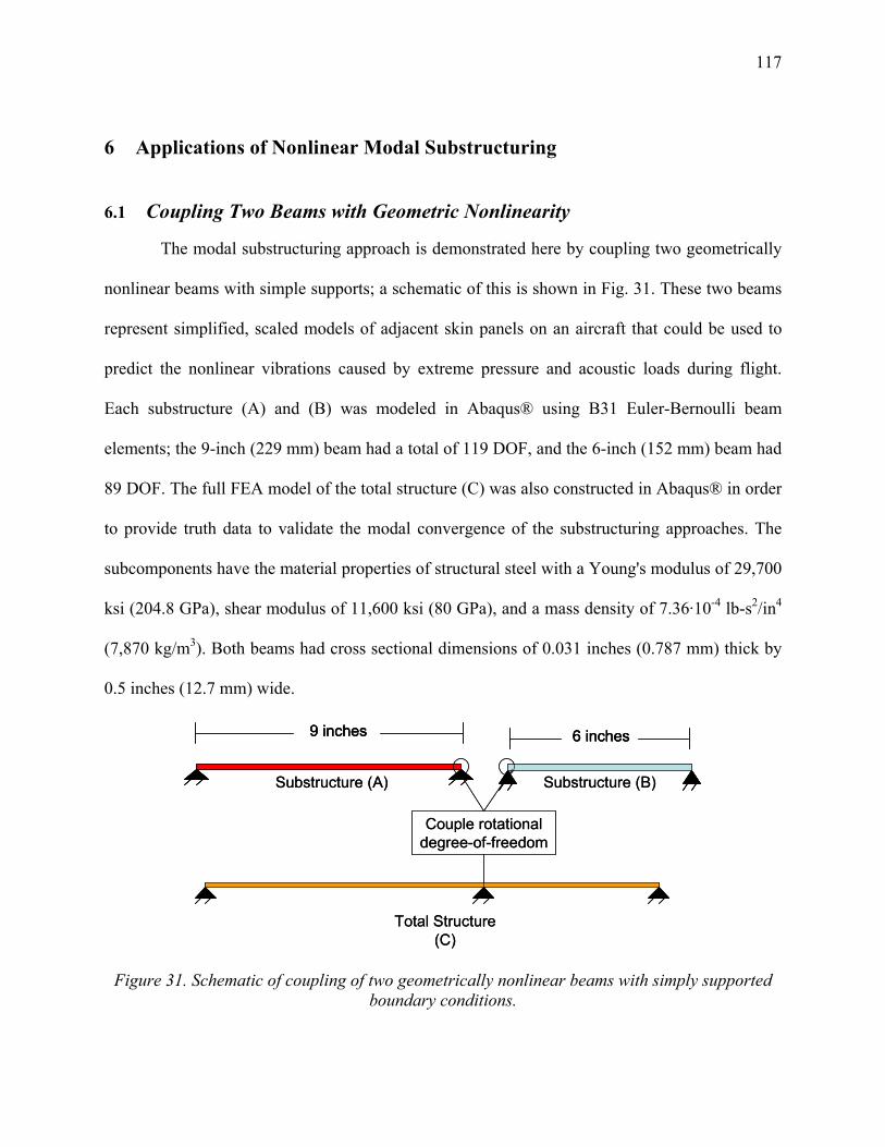
117

6 Applications of Nonlinear Modal Substructuring

6.1 Coupling Two Beams with Geometric Nonlinearity

The modal substructuring approach is demonstrated here by coupling two geometrically

nonlinear beams with simple supports; a schematic of this is shown in Fig. 31. These two beams

represent simplified, scaled models of adjacent skin panels on an aircraft that could be used to

predict the nonlinear vibrations caused by extreme pressure and acoustic loads during flight.

Each substructure (A) and (B) was modeled in Abaqus® using B31 Euler-Bernoulli beam

elements; the 9-inch (229 mm) beam had a total of 119 DOF, and the 6-inch (152 mm) beam had

89 DOF. The full FEA model of the total structure (C) was also constructed in Abaqus® in order

to provide truth data to validate the modal convergence of the substructuring approaches. The

subcomponents have the material properties of structural steel with a Young's modulus of 29,700

ksi (204.8 GPa), shear modulus of 11,600 ksi (80 GPa), and a mass density of 7.36·10-4 lb-s2/in4

(7,870 kg/m3). Both beams had cross sectional dimensions of 0.031 inches (0.787 mm) thick by

0.5 inches (12.7 mm) wide.

Substructure (A) Substructure (B)

Total Structure (C)

Couple rotational degree-of-freedom

9 inches 6 inches

Substructure (A) Substructure (B)

Total Structure (C)

Couple rotational degree-of-freedom

9 inches9 inches 6 inches6 inches

Figure 31. Schematic of coupling of two geometrically nonlinear beams with simply supported boundary conditions.

118

In the following subsection, the modal convergence of two linear substructuring

approaches (i.e. when 0xf NL for each subcomponent model in Eq. (63)) are compared when

using the CB modal basis in Eq. (58), and the other with the free-interface modes in Eq. (55). In

Section 6.1.2, the nonlinear substructuring approach is demonstrated on the same example

problem, except that 0xf NL . The nonlinear subcomponent ROMs with CB modes are

referred as CB-NLROMs, and those created with free-interface modes are referred as NLROMs.

Note that the interface between each beam had only one rotational DOF, therefore each CB basis

required only a single constraint mode, and no reduction at the interface could be performed

using characteristic constraint modes.

6.1.1 Linear Substructuring

The linear models of the 9-inch (229 mm) and 6-inch (152 mm) beams were used to

predict the linear normal modes of the total structure (C) using a free-interface modal

substructuring approach and a Craig-Bampton substructuring approach. One typically includes

modes up to 1.5 to 2.0 times the maximum frequency of interest in the subcomponent ROMs.

The linear natural frequencies for the first thirteen modes (all bending) of each subcomponent

beam model are given in Table 9, along with the exact natural frequencies of the full finite

element model of the total structure (C). The first 5 modes of the total structure are taken to be

the modes of interest, covering a frequency range from 0 to 500 Hz.

119

Table 9. Exact linear natural frequencies of finite element models in Fig. 31.

Simply Support Beam (A): 9 inch Simply Support Beam (B): 6 inch Mode Number Free-Interface Fixed-Interface Free-Interface Fixed-Interface

Total Structure (C)

1 34.85 Hz 54.44 Hz 78.41 Hz 122.5 Hz 42.50 Hz 2 139.4 Hz 176.5 Hz 313.8 Hz 397.3 Hz 97.73 Hz 3 313.8 Hz 368.4 Hz 706.4 Hz 829.5 Hz 162.7 Hz 4 558.2 Hz 630.4 Hz 1,257 Hz 1,420 Hz 313.8 Hz 5 872.7 Hz 962.8 Hz 1,966 Hz 2,170 Hz 382.1 Hz 6 1,258 Hz 1,366 Hz 2,835 Hz 3,080 Hz 588.0 Hz 7 1,714 Hz 1,840 Hz 3,866 Hz 4,153 Hz 762.5 Hz 8 2,241 Hz 2,385 Hz 5,059 Hz 5,389 Hz 930.0 Hz 9 2,840 Hz 3,003 Hz 6,417 Hz 6,791 Hz 1,257 Hz

10 3,511 Hz 3,693 Hz 7,942 Hz 8,361 Hz 1,392 Hz 11 4,256 Hz 4,457 Hz 9,636 Hz 10,100 Hz 1,766 Hz 12 5,074 Hz 5,295 Hz 11,500 Hz 12,020 HZ 2,060 Hz 13 5,966 Hz 6,208 Hz 13,540 Hz 14,110 Hz 2,333 Hz

To be conservative with the target range of 500 Hz, the linear substructuring analysis

started by including subcomponent modes (either free-interface or fixed-interface) with

frequencies up to 1,000 Hz. Additional cutoff frequencies were considered, namely 2,000 and

4,000 Hz, in order to evaluate the modal convergence as additional modes were included in the

basis. These high frequency basis vectors will be especially important for the nonlinear

substructuring case in Section 6.1.2, since higher frequency modes may become coupled to the

lower frequency modes at large response amplitudes. The resulting percent errors of each

predicted natural frequency are given in Table 10 for each linear substructuring approach with

various subcomponent mode frequency ranges. The exact frequencies of the FEA model of the

total structure (C) are used to compute these errors.

120

Table 10. Percent error of the predicted linear natural frequencies of the total structure (C) using subcomponent models that include modes up to 1,000 Hz, 2,000 Hz and 4,000 Hz.

% Error with subcomponent modes up to

1,000 Hz

% Error with subcomponent modes up

to 2,000 Hz

% Error with subcomponent modes up

to 4,000 Hz

Total Structure (C) Mode Number

Free-Interface Modes

CB Modes Free-Interface Modes

CB Modes Free-Interface Modes

CB Modes

1 3.2 5.5·10-4 2.1 5.2·10-4 1.5 5.1·10-4 2 5.5 1.6·10-4 3.5 2.4·10-4 2.4 3.1·10-4 3 9.3 1.9·10-3 5.4 1.3·10-3 3.6 1.2·10-3 4 2.8·10-6 2.5·10-2 3.4·10-6 4.1·10-3 3.7·10-6 4.5·10-4 5 15 3.4·10-3 8.7 1.5·10-3 5.6 1.1·10-3 6 5.2 0.10 2.7 1.6·10-2 1.8 1.4·10-3 7 7.4 0.30 4.2 4.1·10-2 2.8 4.2·10-3 8 N/A 0.22 8.2 2.6·10-2 4.7 2.3·10-3

When including subcomponent modes up to 1,000 Hz, the free-interface approach found

a maximum frequency error of 15 % in the 5th assembly mode. As expected, this basis was not

well suited for this example since the kinematics of the subcomponent do not account for

deformation at the rotational interface [74], and one would need far more free-interface modes

before the basis could begin to properly describe this motion. Interestingly, because the lengths

of the two beams have a ratio 1.5:1, the 4th mode of the assembly is perfectly described by

combining one free-interface mode of each, so its natural frequency is estimated very precisely

using this basis. The CB approach with fixed-interface modes up to 1,000 Hz produced a far

more accurate assembly model because of the kinematics supplied by the constraint modes, and

had a maximum error of 0.30 % for the 7th assembly mode. As expected, out beyond the

frequency range of the CB modal basis the errors become quite large; the error in the 9th and last

predicted mode was 62% (not shown in Table 10).

Including a higher frequency bandwidth, up to 2,000 Hz and 4,000 Hz, improved the

modal predictions with the free-interface approach, however the error was still in excess of 5%

for the 5th mode when including modes up to 4,000 Hz, as compared to 0.0011% for the CB

121

model. These results show that the CB modal basis performs much better than the free-interface

modes, as expected for problems with rigid connections at the interface. For problems with softer

connections (e.g. through rubber grommets as in the auto industry), the free-interface modes

would be expected to perform better.

6.1.2 Nonlinear Substructuring

The nonlinear modal substructuring approaches with the CB-NLROMs and NLROMs

generated with free-interface modes are demonstrated on the example in Fig. 31, but now with

the geometric nonlinearity included in each subcomponent model such that 0xf NL . The

modal convergence of the assembled models was evaluated by comparing its nonlinear normal

modes, which were computed from the assembled equations of motion in Eq. (78) using the

pseudo-arclength continuation algorithm in [49]. The NNMs were also computed from the full

order finite element model of the total structure (C) using the Applied Modal Force (AMF)

algorithm in Chapter 2 to provide a truth solution for comparison.

Figures 32 and 33 show the frequency-energy plots (FEPs) of the first five NNMs, where

the fundamental frequency of the periodic motion is plotted on the vertical axis, and the total

conserved energy (kinetic plus potential) is on the horizontal axis. The energy at which the AMF

results reach a transverse displacement of one beam thickness is marked for reference in Fig. 32.

As noted in the legend, the substructuring results are shown for three cases: two from assembled

CB-NLROMs with fixed-interface modes up to 1,000 Hz and 4,000 Hz, and one with assembled

NLROMs that used free-interface modes up to 4,000 Hz. When generating the static loads to fit

the nonlinear stiffness coefficients of the ROMs, the best practices with the ICE approach in

Chapters 3 and 4 were followed so the CLD scaling factors (from Section 3.5.2) in Eq. (69) were

122

chosen such that a rwmax, was set to 0.25 times the beam thickness, or 7.75·10-3 inches (0.197

mm), and the reduction factor from Section 3.5.2 was used to lower the scale of multi-mode

forces. It was determined that the unconstrained least squares approach in [19] had to be used to

obtain good results with nonlinear substructuring, whereas the results on the monolithic

structures in Chapter 4 were less sensitive and used the constrained least squares approach.

10-6

10-5

10-4

10-3

10-2

10-1

40

45

50

55

60

65

70

75

80

Energy, in-lbf

Fre

quen

cy,

Hz

AMF

CBNLROM- 1,000 Hz

NLROM- 4,000 Hz

CBNLROM- 4,000 Hz

Solution(a)

Solution(b)

Solution(c)

One beamthickness

Figure 32. NNM 1 of the beam assembly using (black circles) AMF on the full FEA model of the total structure (C), (green solid) assembled CB-NLROMs with fixed-interface modes up to 1,000

Hz, (blue dashed) assembled NLROMs with free-interface modes up to 4,000 Hz, and (red dotted) assembled CB-NLROMs with fixed-interface modes up to 4,000 Hz.

The first NNM initiated at the first linear mode solution at low energy, and continued to

higher response amplitudes as energy increased. These elevated response amplitudes introduced

contributions from the nonlinear restoring force, as indicated by the increase in the fundamental

frequency on the vertical axis. This hardening behavior is due to the coupling between the

123

bending and membrane motions, which causes axial stretching when the bending displacements

become large enough. Two distinct features were observed in the FEPs of the first NNM in Fig.

32, namely the main backbone curve and the tongues emanating from this backbone. The main

backbone traced the NNM at the lowest possible energy for a given frequency, and the tongues

indicated the presence of a modal interaction with higher order NNMs at a strict integer ratio of

oscillating frequencies. There were two modal interactions computed with NNM 1 using the

AMF algorithm. For example, the first one initiated around 58 Hz, which started as a 3:1

interaction with NNM 3, meaning that the third mode oscillated at a frequency three times that of

the first mode (note that this time response is shown later in Fig. 34). As the energy increased

along this tongue, another tongue extended from the this one at 68 Hz, resulting in an interaction

where the 4th NNM oscillated at a 5:1 frequency ratio with NNM 1, the 6th NNM oscillated at a

7:1 ratio, all while the 3rd NNM continued to oscillate at the 3:1 ratio.

The main backbone and two modal interactions along NNM 1 were accurately predicted

by the two assembled CB-NLROMs with fixed-interface modes up to 1,000 Hz and 4,000 Hz, as

seen by the agreement with the AMF results. Increasing the number of modes in the CB-

NLROMs did not appear to change the FEP of NNM 1, so either CB-NLROM model could be

confidently used. The assembled NLROMs with free-interface modes up to 4,000 Hz also

performed quite well, but was not as accurate as the assembled CB-NLROMs. At low energy,

there was slight disagreement in frequency, exactly as predicted by the linear substructuring

results in the prior subsection. As the energy increased and the backbone started to bend up in

frequency, the assembled NLROMs accurately matched the main backbone of NNM 1.

However, the tongues emanating from this backbone were not as accurate, and the assembled

NLROM model predicted two new modal interactions that were not present with either the AMF

124

algorithm or the CB-NLROMs. Since these interactions are strongly dependent on the accuracy

of the higher order NNMs involved, these spurious tongues likely came about because the higher

NNMs in the NLROM were not sufficiently accurate. Some of the higher NNMs of the assembly

are plotted in Fig. 33.

10-6

10-5

10-4

10-3

10-2

10-1

100

150

200

250

300

350

400

450

500

Energy, in-lbf

Fre

quen

cy,

Hz

AMF

CBNLROM- 1,000 Hz

NLROM- 4,000 Hz

CBNLROM- 4,000 Hz

Figure 33. NNMs 2 through 5 of the beam assembly, see caption in Fig. 32 for further detail.

The higher order NNMs, spanning frequencies up to 500 Hz, offer similar conclusions as

those seen with the first NNM. Again the FEPs computed with the assembled CB-NLROMs

matched very well with FEPs computed with the AMF algorithm. Either CB-NLROM seems

adequate, although on NNM 5 the lower order model was unable to predict a modal interaction at

425 Hz. Further investigation revealed that this was a 3:1 modal interaction with NNM 9. In

Section 6.2.1 it was found that the 9th predicted linear assembly mode was in error of 62 % when

125

using CB modes up to 1,000 Hz, so it makes sense that this modal interaction would be

erroneously predicted. Other than that, there was little difference between the assembled CB-

NLROM results with the 1,000 Hz and 4,000 Hz bandwidth, suggesting that both would be

adequate for response prediction.

Again the assembled NLROMs with free-interface modes were initially in error at low

energy but predicted each NNM quite well as the branch bent upwards in frequency. The modal

interactions predicted by these models were not as accurate as the assembled CB-NLROMs for

NNMs 2 through 5. As noted previously, because the beam lengths had a 1.5:1 ratio, the fourth

linear mode of the assembly was estimated perfectly by the free-interface mode basis. Here one

also observes that the corresponding 4th NNM is also estimated very precisely using this same

basis. The fifth NNM is significantly in error even though the NLROMs included linear modes

up to 4,000 Hz. These results would be improved with additional free-interface modes in the

basis set, but this was not explored in this work as more modes in the basis would increase the

number of static loads needed to extract the NLROM from the finite element model.

Here the assembled CB-NLROMs had either 9 or 17 DOF, and needed a total of 296 and

1,940 load cases, respectively, to create the ROMs of each subcomponent. For example, the CB-

NLROM under 1,000 Hz had a 6-mode ROM for the 9-inch beam (5 fixed-interface below 1,000

Hz plus 1 constraint mode), and required 232 static load cases. For the 6-inch beam, the CB-

NLROM with 4 modes (3 fixed-interface plus 1 constraint) needed 64 static loads. Thus, the CB-

NLROM eventually had 9 DOF after coupling and required 296 static loads to construct.

Therefore, this equated to approximately 4 minutes of computational time on a desktop computer

with an Intel® Core i7 CPU and 8 GB of RAM, and the 17 DOF model with 1,940 total load

cases took about 15 minutes. The assembled NLROMs had 16 DOF, which required a total of

126

1,538 load cases and 10 minutes of CPU time. Directly building an NLROM of the total structure

(C) with modes up to 4,000 Hz (equivalent to 17 bending modes) would require a total of 6,018

load cases, or 121 minutes. For reference, each NNM curve computed from the FEA model of

the total structure (C) using AMF would take anywhere between 2-4 hours on the computer

mentioned, whereas computing it from any ROM would take approximately 2-4 minutes.

The accuracy of these two nonlinear substructuring approaches was further evaluated by

comparing the time histories at three points on the FEP in Fig. 32, which are marked as solutions

(a), (b) and (c). When comparing the NNMs, the solution at the same energy level as the AMF

solution was selected for the NNM of each assembled ROM. Solutions (a) and (c) were chosen

to show how the response evolved along the main backbone as energy in the response increased,

and solution (b) shows a response on one of the tongues in order to highlight how the beam

vibrates during a modal interaction. The physical response over one period was projected onto

the predicted linear modes of the assembly, which were first normalized to a unit maximum

displacement in order to give the resulting modal amplitudes units of inches, and the resulting

time histories of the three most dominant modes are shown in Fig. 34.

127

0 0.01 0.02-0.02

0

0.02M

odal

Am

plitu

de, i

nch

AMF

0 0.01 0.02-0.02

0

0.02NLROM

0 0.01 0.02-0.02

0

0.02CB-NLROM

0 0.01-0.05

0

0.05

Mod

al A

mpl

itude

, inc

h

0 0.01-0.05

0

0.05

0 0.01-0.05

0

0.05

0 0.0050.01-0.05

0

0.05

Time, s

Mod

al A

mpl

itude

, inc

h

0 0.0050.01-0.05

0

0.05

Time, s

0 0.0050.01-0.05

0

0.05

Time, s

Solution (a) Solution (a)Solution (a)

Solution (b) Solution (b)Solution (b)

Solution (c) Solution (c)Solution (c)

Figure 34. Time histories of the three responses marked on NNM 1 in Fig. 32, where the physical response was projected onto the unit displacement normalized modes of the assembly. The lines represent the three most dominant modes in these responses: (red) mode 1, (blue) mode 2, and

(green) mode 3. Each model included subcomponent modes up to 4,000 Hz.

The time histories of solutions (a) and (c) along the backbone of NNM 1 reveal that the

first linear mode dominates the response, and the results predicted by the assembled NLROMs

and CB-NLROMs agree very well, although the frequency of the assembled NLROMs at point

(a) was slightly higher. Solution (b) occurred along the 3:1 interaction with NNM 3, explaining

128

why the third bending mode oscillated at a frequency three times that of the fundamental

frequency dominated by mode 1. The assembled CB-NLROMs and NLROMs predicted the

response at this modal interaction very well in comparison to the AMF result, although there was

slight disagreement with the frequency and maximum amplitudes predicted by the assembled

NLROMs. Even at locations where the FEP seems to be in slight disagreement, the time history

of the assembled NLROMs appeared to have good accuracy.

Figure 35 compares the maximum deformation shapes of the beam assembly (i.e. when

all DOF have zero velocity) for each of the marked solutions in Fig. 32. The color bar for each

deformation shows the log of the in-plane displacement magnitude at each node (note that the in-

plane displacements were typically a thousand times smaller than the transverse). For the

nonlinear modal substructuring methods, the membrane displacements had to be expanded using

the expansion approach reviewed in Section 3.7 for the CB-NLROMs and NLROMs, since all of

the subcomponent modes used to build the ROMs were bending modes.

129

Figure 35. Maximum deformation shapes of NNM 1 in Fig. 32 using the (left column) AMF algorithm, (middle column) assembled NLROMs with free-interface modes up 4,000 Hz and

(right column) assembled CB-NLROMs with fixed-interface modes up 4,000 Hz. The color bar gives the log of the absolute value of in-plane displacement at each node.

The deformation shapes and the magnitude of the in-plane displacements computed with

both the NLROM and CB-NLROM approaches are in very good agreement with the NNMs

computed with AMF. However, there was one notable difference between the NLROM and

AMF predictions in solution (b) near the support on the left end of the beam. Both the shape and

130

the amount of axial stretching at this location are somewhat inaccurate and this could pose a

problem if this was a region where failure was likely. The CB-NLROM method agreed very

closely with AMF at most points, clearly showing its capability of predicting these in-plane

displacements using the expansion approach, allowing for more accurate modeling of the

stresses. A summary of the maximum percent error in the transverse and in-plane displacements

is provided in Table 11.

Table 11. Maximum percent error of in-plane and transverse displacement of solutions in Fig. 35.

Maximum % Error CB-NLROMs Maximum % Error NLROMs Solution Index In-plane Transverse In-plane Transverse

(a) 2.34 0.137 2.76 0.535 (b) 0.169 0.0405 2.18 2.91 (c) 0.632 0.0450 1.39 0.428

The CB-NLROM substructuring approach is capable of producing highly accurate

predictions of the NNMs, even when including fixed-interface modes up to only 2.0 times the

bandwidth of interest. While the assembled NLROMs built with free-interface modes were much

less accurate, it also gave quite acceptable results for many of the NNMs over much of the

frequency range of interest. In the next section, the CB-NLROM approach is demonstrated on

another example where a modifying element was attached to one of the axial DOF of a 9-inch

(229 mm) long beam.

6.2 Coupling Geometrically Nonlinear Beam to Axial Spring Element

The CB-NLROM modal substructuring technique is now demonstrated on a structural

modification problem where a linear spring element was coupled to a geometrically nonlinear

beam, as shown in Fig. 36. This example again represents a simplified model of an aircraft panel

but instead with in-plane elastic boundary conditions. The geometrically nonlinear beam studied

131

here was 9 inches (229 mm) in length, with a cross section of 0.5 inches (12.7 mm) wide by

0.031 inches (0.787 mm) thick. The Abaqus® model was modeled with forty B31 Euler-

Bernoulli beam elements, resulting in a total of 120 DOF. It was constructed of the same

structural steel used in Section 6.1. The modifying axial spring attached to the left end had a

stiffness of Kax = 25,575 lbf/inch (4,479 kN/m), which was half of the axial stiffness of the beam.

The full FEA model of the geometrically nonlinear beam connected to the in-plane spring was

also constructed in Abaqus® in order to compute the true NNMs of the assembly using the AMF

algorithm.

Note that the assembly of NLROMs with free-interface modes would not work with this

particular example, since the modal basis would only consist of bending type free-interface

modes. For flat beams, the bending motions are completely decoupled from any axial motion, so

these shapes have zero entries for each axial DOF. As a result, coupling an axial element through

a bending only basis would not change the stiffness of the assembled equations. In theory, one

could augment a set of axial modes to the basis, but this was not explored in this work. The CB-

NLROM approach accounts for the in-plane kinematics explicitly with a single constraint mode,

which is the shape resulting from a unit displacement applied to the axial DOF at the left end of

the beam.

Substructure (A)

9 inchesKax

+

Substructure (A)

9 inches9 inchesKax

+

Figure 36. Schematic of the modification of a geometrically nonlinear beam with an axial spring

element having a stiffness of Kax = 25,575 lbf/in (4,479 kN/m).

The fixed-interface modes for the beam in Fig. 36 were exactly those of the free-interface

modes of the 9-inch (229 mm) simply supported beam studied in Section 6.1; the linear natural

132

frequencies of those modes were given in Table 9. The bandwidth of interest for the assembly of

the nonlinear beam and spring is 500 Hz. Once again, two CB models were created including

fixed-interface modes up to 1,000 Hz and 4,000 Hz. Substructuring was then used to assemble

these models to the axial spring to obtain a model for the structure of interest. The first three

NNMs were then computed from the modified CB-NLROMs and are shown below in Fig. 37.

The CLD scaling factors from Section 3.5.2 for the loads in Eq. (69) were chosen such that a

rwmax, was set to 0.25 times the beam thickness for each fixed-interface mode (which were all

bending), and 0.001 times the beam thickness for the one axial constraint mode. The in-plane

nature of the constraint mode warrants a much smaller forcing amplitude compared to the fixed-

interface bending modes. When the constraint mode was forced by a large amount, for example

on the order of 0.25 times the beam thickness, the static solutions in the FEA software would not

converge.

133

10-5

10-4

10-3

10-2

10-1

50

100

150

200

250

300

350

400

450

Energy, in-lbf

Fre

quen

cy,

Hz

AMF

CBNLROM- 1,000 Hz

CBNLROM- 4,000 Hz

Solution (a)

Solution (b)

One beam thickness

One beam thickness

One beam thickness

Figure 37. NNMs 1 through 3 of the modified nonlinear beam using (black circles) AMF on the

full FEA model, and assembled CB-NLROMs with fixed-interface modes up to (green solid) 1,000 Hz, and (red dotted) 4,000 Hz.

The backbones of each NNM predicted by the two assembled CB-NLROMs agree very

well with the AMF results, and these ROMs even captured the modal interaction along NNM 2,

starting at 201 Hz, which was a 3:1 interaction with NNM 4. The agreement between the 1,000

Hz basis and 4,000 Hz basis showed that the CB-NLROMs sufficiently converged with

subcomponent modes up to 2.0 times the frequency of interest so it was not necessary to include

modes up to 8.0 times the frequency range of interest. Of course, other modal interactions could

emerge along these NNMs, as seen with the results in the previous section, and would require a

larger basis set to capture the higher order NNMs involved in the interaction. The maximum

deformation shape of the beam for the solutions marked, (a) and (b), in Fig. 37 are shown in Fig.

38. The membrane displacements were again recovered using the expansion process reviewed in

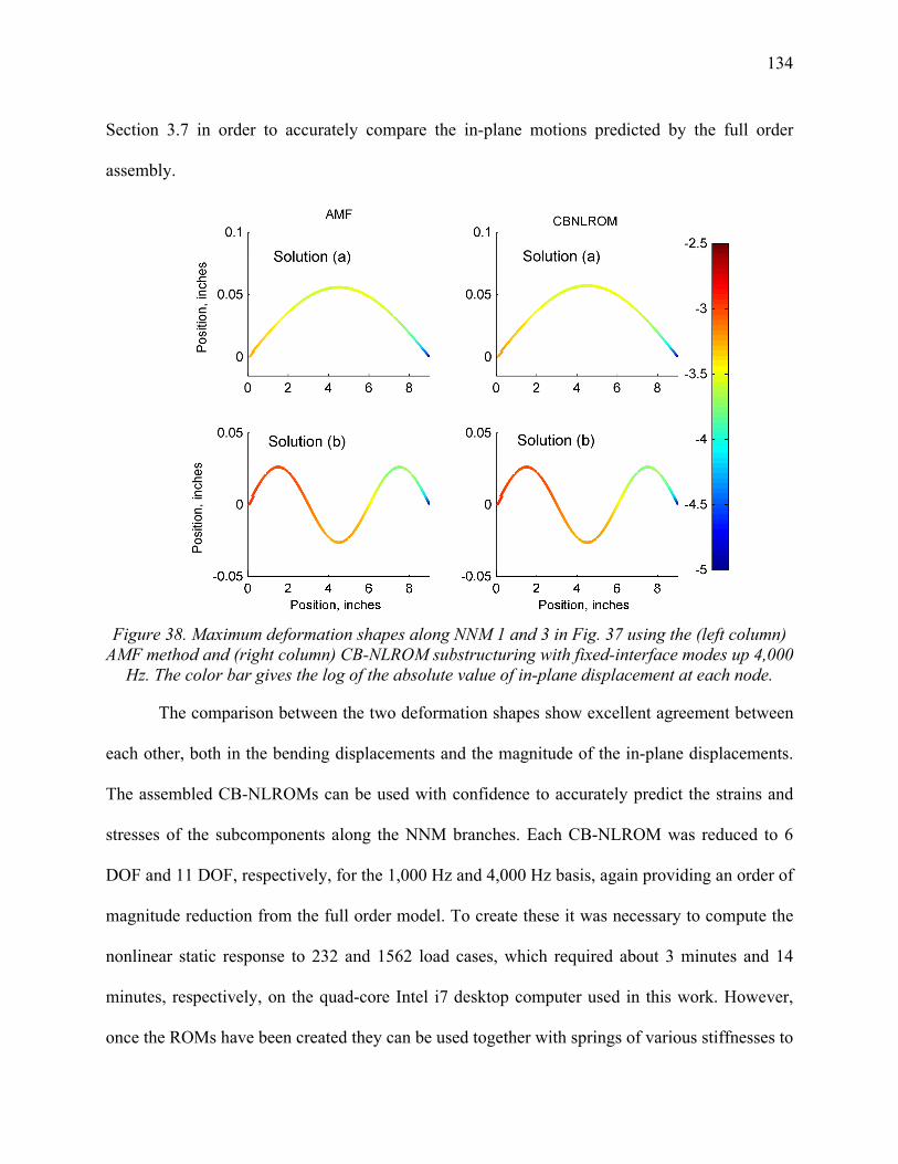
134

Section 3.7 in order to accurately compare the in-plane motions predicted by the full order

assembly.

Figure 38. Maximum deformation shapes along NNM 1 and 3 in Fig. 37 using the (left column)

AMF method and (right column) CB-NLROM substructuring with fixed-interface modes up 4,000 Hz. The color bar gives the log of the absolute value of in-plane displacement at each node.

The comparison between the two deformation shapes show excellent agreement between

each other, both in the bending displacements and the magnitude of the in-plane displacements.

The assembled CB-NLROMs can be used with confidence to accurately predict the strains and

stresses of the subcomponents along the NNM branches. Each CB-NLROM was reduced to 6

DOF and 11 DOF, respectively, for the 1,000 Hz and 4,000 Hz basis, again providing an order of

magnitude reduction from the full order model. To create these it was necessary to compute the

nonlinear static response to 232 and 1562 load cases, which required about 3 minutes and 14

minutes, respectively, on the quad-core Intel i7 desktop computer used in this work. However,

once the ROMs have been created they can be used together with springs of various stiffnesses to

135

very quickly evaluate how the axial boundary condition changes the NNMs or to compute the

response of the structure. Hence, one could save many hours of computation by using the

substructuring approach to perform design studies, even for this relatively simple structure.

6.3 Coupling Two Plates with Geometric Nonlinearity

The modal substructuring approach was applied to the assembly of two geometrically

nonlinear, flat plates coupled to one another along a continuous interface. Each plate had simple

supports at all nodes around the edges, and was modeled in Abaqus®. A schematic of these FEA

models is shown in Fig. 39, where the two substructures were coupled at all x, y, and z rotational

DOF along a shared edge. The 9 inch by 9 inch (229 mm by 229 mm) plate was modeled with

1,296 S4R shell elements (a 3636 grid), while the 9 inch by 6 inch (229 mm by 152 mm) plate

had a total of 864 S4R shell elements. Each plate had a uniform thickness of 0.031 inches (0.787

mm); thin-walled structures such as these can experience large deformations even while the

materials remain within their linear elastic range. The material properties were those of structural

steel having a Young's modulus of 29,700 ksi (204.8 GPa), shear modulus of 11,600 ksi (80

GPa), and mass density of 7.36·10-4 lb-s2/in4 (7,870 kg/m3). A total of 37 nodes were along the

connection points, meaning there were 111 DOF at the interface.

136

9 inches(229 mm)

Subcomponents Total Structure

Couple at x, y and z rotational DOF

9 inches(229 mm) 6 inches

(152 mm)15 inches(381 mm)

9 inches(229 mm)

Subcomponents Total Structure

Couple at x, y and z rotational DOF

9 inches(229 mm) 6 inches

(152 mm)6 inches

(152 mm)15 inches(381 mm)

Figure 39. Schematic of coupling two geometrically nonlinear plates with simple supports at all edges. The FEA model of the total structure has simple supports at all edges and DOF along the

red line where to two plates join.

In Section 6.3.1, the modal convergence of a linear substructuring approach (i.e. when

0xf NL for each subcomponent model in Eq. (63)) is performed using the fixed-interface

modes with characteristic constraint modes in Eq. (62) and the Craig-Bampton modal basis in

Eq. (58). In Section 6.3.2, the nonlinear substructuring approach is demonstrated on the same

example problem, except that 0xf NL . The nonlinear subcomponent ROMs with fixed-

interface and characteristic constraint (CC) modes are referred as CC-NLROMs. Note that the

interface between the plates had 111 rotational DOF/constraint modes, therefore the CB basis

would require far to many static load cases to fit a nonlinear ROM with Implicit Condensation

and Expansion, so this approach was not pursued on this problem.

6.3.1 Linear Substructuring

The linear FEA models of the plates were first used to determine how many characteristic

constraint modes would be needed for the linear substructuring problem, which provides insight

into the basis selection for the nonlinear substructuring problem. Table 12 gives the natural

frequencies and mode shapes of the fixed-interface and characteristic constraint modes for each

subcomponent model. The exact modes of the full FEA model of the assembly are shown in the

137

far right column to provide a reference solution against which to compare the substructuring

results that will be presented later.

138

Table 12. Linear subcomponent modes used with the CC mode reduction.

Mode Number

Fixed-interface modes: 9”x9” plate

Fixed-interface modes: 9”x6”

plate Characteristic

constraint modes Truth modes of total

structure

1 87.1 Hz 156.8 Hz 140.2 Hz 78.4 Hz

2 190.6 Hz 254.4 Hz 420.9 Hz 135.1 Hz

3 216.6 Hz 430.1 Hz 930.7 Hz 185.7 Hz

4 317.7 Hz 449.5 Hz 1660 Hz 203.0 Hz

5 371.4 Hz 547.0 Hz 2610 Hz 239.5 Hz

6 420.3 Hz 685.2 Hz 3785 Hz 306.4 Hz

7 494.6 Hz 717.4 Hz 5196 Hz 365.7 Hz

8 521.5 Hz 915.3 Hz 6853 Hz 368.2 Hz

9 630.0 Hz 965.6 Hz 8769 Hz 419.7 Hz

10 696.1 Hz 1014 Hz 10.96 kHz 434.1 Hz

11 700.6 Hz 1021 Hz 13.44 kHz 474.4 Hz

12 749.8 Hz 1183 Hz 16.24 kHz 485.5 Hz

139

For this example, the frequency range of interest was 0-500 Hz, so the first 12 modes of

the total structure in Table 12 were taken as target modes. A typical rule of thumb for linear

substructuring is to include subcomponent modes up to 1.5 to 2.0 times this range. Even though

the characteristic constraint modes have associated eigenfrequencies from the secondary modal

analysis in Eq. (61) in Section 5.2.3, this rule of thumb is not well established for these modes.

When deciding which CC modes to retain in the basis, it was determined that these should be

selected such that the accuracy of the CB substructuring approach was preserved. This was done

by computing the maximum percent frequency errors between the modes predicted by the

assembled CB ROMs, and those from the assembly of truncated CC ROMs. This is demonstrated

on the linear plates with subcomponent fixed-interface modes up to 750 Hz, 1,000 Hz and 1,500

Hz, or 1.5, 2.0 and 3.0 times the frequency band of interest, respectively. The maximum of the

percent frequency error between all modes predicted by the assembled CC ROMs and the

assembled CB ROMs is shown in Fig. 40 as CC modes were added to the basis. As the number

of CC modes increases the error precipitously falls down below 0.01%, hence for each case the

number of CC modes included was chosen such that the maximum percent error in the linear

frequencies fell below 0.01 %. Returning to Table 12, one can see that the maximum frequency

of the CC modes that were included is well beyond the frequency range of interest in each case.

140

1 2 3 4 5 6 7 810

-4

10-3

10-2

10-1

100

101

Number of CC modes

Ma

xim

um %

fre

quen

cy e

rror

750 Hz

1,000 Hz

1,500 Hz

Figure 40. Maximum percent error of the assembly modes predicted by the CB ROMs and the

CC ROMs as the number of CC modes were increased in the basis. The lines represent the number of fixed-interface modes included in each ROM: up to (red squares) 750 Hz, (blue

circles) 1,000 Hz and (green asterisks) 1,500 Hz.

Hence, four, five and six CC modes were included in the CC ROM basis for the cases

where the fixed-interface modes were included up to 750 Hz, 1,000 Hz, and 1,500 Hz,

respectively. Even after truncating the CC modes in this manner, the resulting model still

provides the same predictive accuracy as the full assembled CB ROMs, which have 111

constraint modes. The total number of DOF in each of these reduced order models was then 23,

30, and 44 DOF. The percent frequency errors in Table 13 compare the predicted modes with

those of the full FEA model of the total structure, providing insight into the accuracy of these

assembled CC ROMs (and ultimately the CB substructuring approach). The lowest order ROM

predicted the assembly modes up to 500 Hz very well including linear modes up to only 1.5

times the frequency band of interest; the largest frequency error was 0.39 % in the 11th mode.

Additional modes in the basis lowered the frequency error further, as expected.

141

Table 13. Percent frequency error of the first 12 assembly modes predicted by the assembled CC ROMs and the full FEA model of the total structure.

Total Structure Mode Number

% Error with 4 CC modes and up to 750 Hz

fixed-interface modes

% Error with 5 CC modes and up to 1,000 Hz fixed-

interface modes

% Error with 6 CC modes and up to 1,500 Hz fixed-

interface modes 1 4.4·10-4 1.7·10-4 6.7·10-5 2 7.2·10-3 4.8·10-3 4.0·10-3 3 1.2·10-3 -1.8·10-4 -1.3·10-3 4 7.4·10-3 4.0·10-3 2.8·10-3 5 1.4·10-2 6.8·10-3 8.5·10-4 6 1.9·10-2 9.8·10-3 2.3·10-3 7 0.16 6.2·10-2 2.7·10-2 8 5.7·10-3 3.8·10-3 1.7·10-3 9 2.0·10-2 1.1·10-2 2.1·10-3

10 1.5·10-2 5.7·10-3 2.4·10-3 11 0.39 0.18 3.3·10-2 12 2.4·10-2 1.3·10-2 3.1·10-3

For a linear system, the CC ROMs with modes up to 750 Hz and 4 CC modes would be

sufficient for response prediction. In the next subsection, all of these bases are used to compare

the nonlinear substructuring approach since additional modes might be necessary to capture the

dynamics of the nonlinear assembly. The same modal bases are used when generating the CC-

NLROMs of the geometrically nonlinear plates in Fig. 39, and the convergence of the nonlinear

substructuring results is evaluated using nonlinear normal modes.

6.3.2 Nonlinear Substructuring

The CC-NLROMs of the two plate models were generated with the same set of fixed-

interface and characteristic constraint modes used in the linear analysis (fixed-interface modes up

to 750 Hz, 1,000 Hz and 1,500 Hz with 4, 5 and 6 CC modes, respectively). The force

amplitudes f̂ for the static loads in Eq. (69) are typically chosen such that when a single-mode

force (e.g. rrCCr f̂,KTF ) is applied to the linear FEA model, the maximum displacement is on

the order of one thickness. For the CC-NLROMs generated here, each mode in the CCT basis in

Eq. (62) was scaled to force the linear system to a maximum displacement of 0.25 times the

142

thickness, or 7.75·10-3 inches (0.197 mm). The details on the scaling are found in Section 3.5.2.

Once the coefficients in Eq. (68) were identified, the CC-NLROMs were coupled and the

equations of motion in Eq. (78) were used to compute the NNMs using the pseudo-arclength

continuation algorithm in [49]. The first three NNMs of the assembled CC-NLROMs are

compared with the NNMs of the full FEA model of the total structure in Fig. 41. The full order

model NNMs were computed using the applied modal force (AMF) algorithm Chapter 2, but

these curves were quite expensive since the model had >10,000 DOF. These provide a few

reference solutions along the backbone to help validate the accuracy and convergence of the

assembled CC-NLROMs, analogous to the comparison of linear normal modes in the previous

subsection.

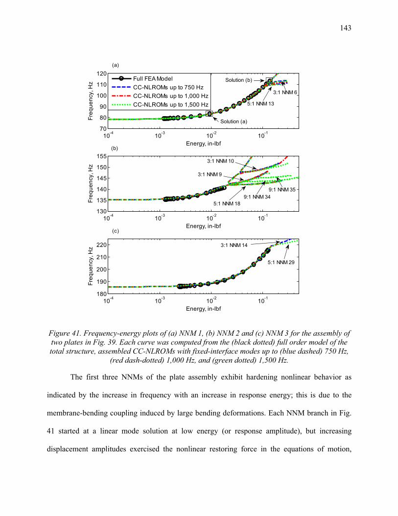
143

10-4

10-3

10-2

10-1

70

80

90

100

110

120

Energy, in-lbf

Fre

qu

en

cy, H

z

Full FEA Model

CC-NLROMs up to 750 Hz

CC-NLROMs up to 1,000 Hz

CC-NLROMs up to 1,500 Hz

10-4

10-3

10-2

10-1

130

135

140

145

150

155

Energy, in-lbf

Fre

qu

en

cy, H

z

10-4

10-3

10-2

10-1

180

190

200

210

220

Energy, in-lbf

Fre

qu

en

cy, H

z

5:1 NNM 29

3:1 NNM 14

3:1 NNM 9

3:1 NNM 10

Solution (a)

3:1 NNM 6

5:1 NNM 13

5:1 NNM 189:1 NNM 34

9:1 NNM 35

Solution (b)

(a)

(b)

(c)

Figure 41. Frequency-energy plots of (a) NNM 1, (b) NNM 2 and (c) NNM 3 for the assembly of two plates in Fig. 39. Each curve was computed from the (black dotted) full order model of the total structure, assembled CC-NLROMs with fixed-interface modes up to (blue dashed) 750 Hz,

(red dash-dotted) 1,000 Hz, and (green dotted) 1,500 Hz.

The first three NNMs of the plate assembly exhibit hardening nonlinear behavior as

indicated by the increase in frequency with an increase in response energy; this is due to the

membrane-bending coupling induced by large bending deformations. Each NNM branch in Fig.

41 started at a linear mode solution at low energy (or response amplitude), but increasing

displacement amplitudes exercised the nonlinear restoring force in the equations of motion,

144

changing the dynamic response. There are two notable features of the NNM branches in Fig. 41,

namely the backbone, which occurs at the lowest possible energy for a given frequency, and the

tongues, which emanate from the backbone. Each tongue corresponds to a modal interaction with

other NNMs of the model that oscillate at a strict integer ratio of frequencies (see [25, 38] for

further discussion of these solutions). AMF was run in a manner that caused all of its solutions

(black circles) to remain along the main backbone; further computations would be needed to

capture these modal interactions.

The main backbones predicted by all of the assembled CC-NLROMs agree very well

with those of the full order model, suggesting that even the lowest order model (with fixed-

interface modes up to 750 Hz and 4 CC modes) could be used for accurate response prediction.

Adding fixed-interface and CC modes to the basis did slightly affect the modal interactions

predicted by the ROMs. For example, in Fig. 41c the modal interaction near 220 Hz started as a

3:1 interaction with NNM 14 (i.e. mode 14 oscillates at a frequency 3 times the fundamental

frequency of ~220 Hz). The 750 Hz assembly of CC-NLROMs (blue dashed) continued along

this tongue towards higher energies, whereas the 1,500 Hz assembly (green dotted) continued

along a new tongue corresponding to a 5:1 interaction with NNM 29. Since the 750 Hz model

only had 23 DOF it would not be able to capture NNM 29, meaning that higher order ROMs

were needed to capture this tongue. Similar observations are made in Fig. 41b with the tongues

emanating from the 3:1 interaction with NNM 9. The 1,500 Hz assembly of CC-NLROMs

captured the 9:1 interactions with NNMs 34 and 35, both of which were not captured with the

lower order models. An infinite number of these interactions can occur along the backbone of the

NNM, and it is hard to determine the effect of these solutions on the accuracy of the ROMs and

their intended use.

145

The higher order NNMs 4 through 10 computed with the 750 Hz and 1,500 Hz models

were all in agreement along the backbones, however NNM 11 was the first to show a slight

offset between the two models (these results are not shown for brevity). The nonlinear modal

convergence study helps identify when a sufficient number of modes have been included in the

basis for the frequency bandwidth of interest. To further compare each model, the maximum out-

of-plane displacements (i.e. when the velocity is zero) are shown in Table 14 for the solutions

marked (a) and (b) in Fig. 41a, showing how the deformation shapes evolve along the backbone

of NNM 1. The deformations predicted by the models agree very well with one another, as

expected from the agreement with the frequency-energy plots shown earlier. The deformation

shapes changed as the energy increased along the backbone showing that more vibration energy

was in the smaller 9 inch by 6 inch (229 mm by 152 mm) plate at solution (b) as compared with

solution (a), which was taken near the linear regime. The shapes all agree very well suggesting

that either CC-NLROM would adequately capture the response of the assembly near these two

points.

146

Table 14. Table comparing the out-of-plane maximum deformation shapes of solutions (a) and (b) marked along NNM 1 in Fig. 41.

Model Solution (a) at 83.2 Hz Solution (b) at 112.9 Hz

Full Order Model

CC-NLROMs with modes up to 750 Hz

CC-NLROMs with modes up to 1,500 Hz

The NNMs computed from the undamped equations of motion in Eq. (78) have an

intimate connection to the forced steady state response of the damped system, as these undamped

NNMs form the backbone to the forced response curves as discussed in Section 1.2. Resonance

of the damped response occurs in the neighborhood of the NNM when the damping forces

exactly cancel out the harmonic forcing function. Therefore, by accurately capturing the NNMs,

the damped forced response near resonance, which is when the structure is at its greatest risk of

failure, will also be accurate. Hence, the results presented above suggest that either of the CC-

NLROMs would accurately capture the forced response of the panel near resonance.

During the course of this research, it was questioned whether it was truly important to

capture the nonlinear stiffness of the characteristic constraint modes and their nonlinear

147

couplings to the other modes. It was hypothesized that these terms might be negligible, in which

case one could simply create a ROM from the fixed-interface structure, augment it with

traditional, linear CC modes, and compute the response of the assembly. To test this hypothesis,

a separate modeling strategy was explored during this research where each nonlinear

subcomponent ROM was estimated fixing all of the boundary DOF in the FEA model in Eq.

(63), computing the nonlinear modal model from it using only the fixed-interface modes, and

appending the linear CC modes. These subcomponent models are referred to here as fixed-

interface NLROMs (FI-NLROMs), and were assembled in the same way as the CC-NLROMs in

Section 5.4. This approach was motivated by the potential computational savings obtained by

only requiring static force permutations in Eq. (69) in the shapes of the fixed-interface modes,

and not the static constraint modes. For example, for the ROMs of the 9 by 9 inch (229 mm by

229 mm) plate with fixed-interface modes up to 1,500 Hz, this would require only 15,226 load

cases instead of 30,914 for the CC-NLROM. Unfortunately, this approach was found to produce

an inaccurate estimate of the first NNM, as shown in Fig. 42.

148

10-4

10-3

10-2

10-1

70

75

80

85

90

95

100

105

110

115

120

Energy, in-lbf

Fre

que

ncy,

Hz

Full FEA Model

FI-NLROM up to 1,500 Hz

CC-NLROM up to 1,500 Hz

Figure 42. Frequency-energy plots of NNM 1 for the assembly of two plates. Each curve was computed from (black dotted) full order model of the total structure, (green dotted) assembled

CC-NLROMs and (purple solid) assembled FI-NLROMs with fixed-interface modes up to 1,500 Hz.

The NNM predicted by the assembled FI-NLROMs with fixed-interface modes up to

1,500 Hz (and 6 linear CC modes) clearly disagrees with that predicted by the assembled CC-

NLROMs with the same basis and the reference solutions from the full FEA model. In order to

quantify the importance of these results, the energy balance technique in [38, 55, 56] was used to

compute the force amplitude required to excite resonance of the damped system with a single-

point harmonic forcing function. In this calculation, each mode of the FI-NLROMs and CC-

NLROMs was assumed to have 0.1% modal damping, which is near the damping level observed

experimentally for similar structures [19]. A point force was applied at the midpoint of the 9 inch

by 9 inch (229 mm by 229 mm) plate in the out-of-plane direction. This analysis predicted that a

point force with an amplitude of 9.6·10-3 lbf (4.3·10-2 N) would excite resonance of the

assembled FI-NLROMs at 90 Hz, resulting in a peak displacement of 0.0328 inches (0.833 mm).

The calculations with the more accurate ROM predicted that this force amplitude would actually

149

produce resonance at a significantly higher frequency (104.3 Hz) with a smaller peak

displacement of 0.0295 inches (0.749 mm). The corresponding locations are marked with an (+)

in Fig. 42. The accuracy of the modeling strategy and its resulting NNMs have a strong

connection to the accuracy the various forced response predictions.

The AMF algorithm took on the order of 2 to 3 days to compute each NNM of the 12,861

DOF full order model of the assembly using a desktop computer with an Intel® Core i7 CPU and

8 GB of RAM, so only a few "truth" solutions were available for comparison throughout this

section. Each NNM from the CC-NLROM substructuring approach took anywhere from 15-30

minutes to compute, depending on the parameters used in the stepsize controller and the size of

the ROM. The upfront cost to run the static analyses for each CC-NLROM is summarized in

Table 15, along with the cost estimate if all 111 static constraint modes were used in the basis

without any interface reduction (note that this would be the CB-NLROM approach used in

Sections 6.1 and 6.2). For example, creating the CC-NLROMs with fixed-interface modes up to

1,500 Hz and 6 CC modes would require a total of 42,436 static load cases, taking 46 hours on

the desktop computed mentioned earlier, and the equivalent CB-NLROMs would require

5,808,336 static loads and 248 days of CPU time. The interface reduction reduced the number of

static loads required by ICE approach to identify each subcomponent model, making the modal

substructuring approach feasible. For reference, creating an NLROM of the full plate assembly

using the approach in Chapter 3 with linear modes up to 500 Hz and 1,500 Hz (a total of 12 and

41 modal DOF, respectively) would require 2,048 static loads (4 hours) and 88,642 static loads

(173 hours), respectively. In practice, this model would likely need more than modes up to 500

Hz to accurately capture all the NNMs in the 0-500 Hz frequency range, however this serves as

the lower bound to the cost estimate.

150

Table 15. Computational cost associated with the identification of nonlinear subcomponent models using ICE.

Fixed-interface modes up to 750 Hz

Fixed-interface modes up to 1,000 Hz

Fixed-interface modes up to 1,500 Hz

Model CB-NLROM CC-NLROM CB-NLROM CC-NLROM CB-NLROM CC-NLROM

9 inch by 9 inch plate

·123 DOF ·2,451,226 loads ·122 days

·16 DOF ·4,992 loads ·6 hours

·127 DOF ·2,699,258 loads ·134 days

·21 DOF ·11,522 loads ·14 hours

·134 DOF ·3,172,584 loads ·158 days

·29 DOF ·30,914 loads ·37 hours

9 inch by 6 inch plate

·118 DOF ·2,163,176 loads ·74 days

·11 DOF ·1,562 loads ·1 hour

·120 DOF ·2,275,520 loads ·78 days

·14 DOF ·3,304 loads ·3 hours

·126 DOF ·2,635,752 loads ·90 days

·21 DOF ·11,522 loads ·9 hours

6.4 Summary

This chapter presented three case studies demonstrating the nonlinear modal

substructuring approaches in Chapter 5 on geometrically nonlinear finite element models. The

results on the two geometrically nonlinear beam examples showed that the assembled CB-

NLROMs (built with fixed-interface and constraint modes) reproduced the NNMs of interest

very well when the basis included modes up to twice the frequency band of interest. For the

NLROM method (using free-interface modes), there were still noticeable errors with modes up to

8.0 times the bandwidth, but overall the results agreed well with the truth model and may have

been adequate for many purposes. For applications with softer connections, the free-interface

basis would be expected to perform better. An advantage of the CB-NLROM method is that the

CB basis can readily include axial kinematics, so one can readily perform design studies to

assess the effect of the in-plane stiffness of the mounting structure. One foreseeable pitfall to the

CB modal basis, however, is the fact that it could require a very large number of constraint

modes to capture the kinematics of a continuous interface with many interface DOF, hence

motivating the use of characteristic constraint modes.

The substructuring approach with CC-NLROMs (built with fixed-interface and

characteristic constraint modes) was demonstrated in Section 6.3 by coupling two thin plates

151

with geometric nonlinearity. The NNMs were computed from the assembled CC-NLROMs

generated with an increasing number of fixed-interface and characteristic constraint modes. The

results showed excellent agreement along the backbone predicted by each ROM and the full

order model. The only difference with the higher order ROMs were the modal interactions along

the NNM, which are associated with interactions involving higher order modes. The results

showed how the maximum deformation shapes evolved along the backbone of NNM 1,

providing valuable insight into the evolution of the stress fields experienced by the system at

various resonant conditions. The interface reduction with characteristic constraint modes

drastically reduced the number of DOF describing the interface, hence lowering the upfront

computational cost associated with the identification of the nonlinear stiffness coefficients in the

subcomponent models. The assembly of CC-NLROMs was orders of magnitude smaller

compared to the full order finite element model yet maintain acceptable accuracy.

A substructuring approach has the advantage of dealing with several small, simpler

subcomponent models compared to one large complicated model. Often during the development

and analysis of structural components, most design changes occur at a subcomponent level,

therefore a modal substructuring approach makes it easier to update one subcomponent model

rather than the entire model of the assembly. This work has relied exclusively on the NNMs to

judge the quality of the assembled ROMs. The author and his colleagues advocate the use of this

approach because the NNMs provide a load-independent characterization of the nonlinear model

and yet they have been shown to be intimately connected to the response of the structure to

various types of loading [25, 35, 40, 41]. For all of the cases studied here, the true NNMs were

calculated by the AMF algorithm in Chapter 2, but this algorithm becomes quite expensive for

large finite element models. Fortunately, the results shown here suggest that the NNMs tend to

152

converge as additional modes are added to the subcomponent basis, so the NNMs could be used

as a convergence metric without a comparison to the truth model.

153

7 Conclusions

The dynamic reduction strategies used throughout this work have shown to be very

sensitive to a number of modeling decisions, such as the number and type of modes in the basis,

and the scaling amplitudes of the static loads used to fit the nonlinear stiffness coefficients. In

this dissertation, a novel approach to evaluate the convergence of these geometrically nonlinear

reduced order models was developed based on their undamped nonlinear normal modes. This

work also proposed a modal substructuring framework to create a reduced order model of a

large, complicated structure by first dividing it into smaller subcomponent models, building

ROMs of each using the Implicit Condensation and Expansion approach, and assembling these

by satisfying compatibility and force equilibrium.

The accuracy of candidate ROMs was evaluated in Chapter 4 by comparing the NNMs

from the reduced equations to those computed from the full order FEA model using the Applied

Modal Force (AMF) algorithm in Chapter 2. Two geometrically nonlinear systems were studied

in Chapter 4 with the Implicit Condensation and Expansion and Enforced Displacement

approaches, and valuable insight was revealed about the sensitivities of the scaling methods and

mode selection. The reference NNMs from the full order models provided confirmation that the

ROMs were converging to the true solution, giving confidence in the ability of the NNM to

provide a reliable convergence metric. In the applications of interest (e.g. complicated FEA

models with many DOF), the solution of the full order model will be too expensive to compute,

but the case studies presented here provide guidance regarding the load amplitudes to try and

illustrate how sensitive the results can be to load cases and modal basis selection. A third case

study on a simply supported beam with an impacting spring was presented in Chapter 4 to

154

demonstrate the convergence metric on a system with non-smooth nonlinearities where the

NNMs from the full order model were not available. The ROMs were generated with an

increasing number of linear vibrations modes and a single discontinuous basis function [113],

and the NNMs appeared to converge along the backbone but not along the internal resonances.

The importance of the internal resonances was evaluated by comparing the response of the

ROMs to the full order model for both an impulsive load and a random input. These results

suggest that a ROM that accurately captured the backbone (and also included a similar density of

internal resonances) would be adequate to predict the random and transient response, although no

formal proof was developed in this work.

A nonlinear modal substructuring approach for geometrically nonlinear structures was

developed in Chapter 5 by first creating subcomponent ROMs with the Implicit Condensation

and Expansion method [19, 103] using either free-interface modes, fixed-interface plus

constraint modes, or fixed-interface plus characteristic constraint modes [82]. Once the

subcomponent ROMs were identified, they were assembled to provide a reduced order model of

the global assembly that accounts for geometric nonlinearity. The results in Chapter 6 evaluated

the accuracy of the nonlinear substructuring approaches with three case studies involving

geometrically nonlinear FEA models. The free-interface and fixed-interface plus constraint mode

basis was used to couple two nonlinear beams at a shared rotational DOF, revealing that the

latter basis had better convergence properties. One advantage of the fixed-interface plus

constraint mode basis was that it readily included axial kinematics, so it was demonstrated on a

structural modification problem where a linear spring element was coupled to a geometrically

nonlinear beam at an axial DOF. This approach allows one to modify the in-plane elastic

boundary conditions and assess the effect of the in-plane stiffness on the mounting structure. A

155

final case study involving two geometrically nonlinear plates demonstrated that the size of the

interface could be reduced by more than an order of magnitude using characteristic constraint

modes. For the subcomponent models with 6 CC modes and fixed-interface modes up to 1,500

Hz, this reduced the number of static load cases down to 42,436 (or 46 hours of CPU time) from

the 5,808,336 (248 days) that would have been needed without the interface reduction. An

equivalent ROM created from the full FEA model of the assembly with modes up to 500 Hz and

1,500 Hz would have required 2,048 static load permutations of 12 modes (4 hours) and 88,642

static load permutations of 41 modes (173 hours), respectively. Creating a reduced order model

with substructuring allows one to build ROMs of simpler subcomponent models that could

potentially require fewer modes than the ROM approach on the full order model (Chapter 3),

however this will strongly depend on the number of basis vectors needed to accurately capture

the response.

The NNMs serve as a signature of the equations of motion that clearly and concisely

describe the dynamics of the system, and provide a metric that is independent of external loads

making it ideal for comparisons between a set of candidate ROMs of geometrically nonlinear

FEA models. This dissertation showed that even if the true NNM solutions from the AMF

algorithm from Chapter 2 were not available, the convergence of the NNMs would still provide a

powerful comparison metric. One advantage to the NNM is that they provide valuable insight

into the dynamics of the system and to the response to various load environments. For example,

the intimate connection between the NNMs and the harmonically forced, damped response

suggest that a ROM that is able to accurately predict the NNMs can also predict the resonance of

the lightly damped system [25, 34-39, 55, 56], a situation where the structure will be most likely

to fail. The ROMs of a geometrically nonlinear FEA model can be created either directly from

156

the FEA model of the assembled structure, or from an assembly of subcomponent ROMs. Either

way, the NNMs help to evaluate the accuracy and convergence of the reduce equations to give

the user confidence in the ability of the ROM to make efficient and accurate response

predictions.

157

8 Future Work

8.1 Substructuring of Thermal-Structural Models

The modal substructuring approach developed in this dissertation only applies to the

nonlinear structural model of the system of interest. In extreme load environments during high

speed flight [21, 22], coupled structural-thermal interactions may strongly influence the

nonlinear response and the reduced order model of these structures would need to capture the

appropriate physics (e.g. see [119, 120]). The substructuring framework could be extended to

assemble a set of thermal-structural reduced order models with relatively little variation from the

approach developed in this dissertation. The coupled ROMs would provide more accurate

response predictions if aerothermal effects are expected to influence the response of the global

assembly of interest (e.g. full order model of a high speed aircraft), allowing for more

computationally efficient time simulations of models involving coupled physics.

8.2 Model Updating

This work demonstrated that nonlinear normal modes are valuable as a convergence

metric, since they provide insight into the accuracy of the reduced order models. Recent studies

have used undamped NNMs as an amplitude dependent metric to make comparisons between

experimentally identified NNMs and those predicted by a numerical/analytical model [109, 110].

The nonlinear modal parameters (e.g. energy dependent frequencies, deformation shapes, etc..)

could be used to define an optimization function, or cost function, for a model updating scheme.

Kuether and Allen [121] recently developed an algorithm based on numerical integration and

shooting that validates the NNMs from reduced order models by using the initial conditions from

the ROM as a initial guess to the shooting function in the AMF algorithm in Chapter 2. If the

158

shooting function is satisfied, then this confirms the accuracy of the ROM at a given energy level

without having to run the AMF algorithm on the full model. This shooting algorithm could be

utilized in a model updating algorithm based on the energy dependent modal parameters to

validate the full order, nonlinear finite element model with experimental NNMs.

This new model updating approach would provide insight into how each parameter of the

FEA model affects the nonlinear dynamic response of the structure. The NNMs have an intimate

connection to the forced response and can help guide specific design modifications to obtain the

desired nonlinear response. For example, imagine that a structure is exposed to a large, random

force that strongly excites frequencies near the first NNM. One could modify the characteristics

of the first NNM in the energy range of interest with changes to the structural design to lower the

overall response amplitudes and hence the stress fields that dictate the life of the structure.

8.3 Connection Between NNMs and Response Prediction

Nonlinear normal modes were used throughout this work to identify how changes to the

reduced order model affected the dynamics of the resulting model. The frequency-energy curves

gave qualitative insight into the ability of the model to capture the NNM(s) of the full order

model, however the lack of superposition makes it difficult to find a quantitative connection.

More work is needed to determine which NNMs must be accurate to compute responses due to

various load environments (e.g. transient, random, etc...) and especially to establish a

quantitative link between the accuracy of the NNMs and response metrics of interest. Recently,

Ardeh [33] began to explore the role of NNMs in the reconstruction of a system's response

through the development of connecting functions. His work could eventually lead to this

quantitative connection but for now one should consider quantitative metrics based on the

response while using the nonlinear modes to provide qualitative insight.

159

Appendix – Publications of PhD work

Journal Papers

Kuether, R.J. and M.S. Allen, “A Numerical Approach to Directly Compute Nonlinear Normal

Modes of Geometrically Nonlinear Finite Element Models,” Mechanical Systems and Signal

Processing, vol. 46, pp. 1-15, 2014.

Kuether, R.J., B.J. Deaner, J.J. Hollkamp, and M.S. Allen, “Evaluation of Geometrically Nonlinear

Reduced Order Models with Nonlinear Normal Modes,” AIAA Journal, (submitted).

Kuether, R.J., M.S. Allen, and J.J. Hollkamp “Modal Substructuring of Geometrically Nonlinear

Finite Element Models,” AIAA Journal, (submitted).

Kuether, R.J., M.S. Allen, and J.J. Hollkamp “Modal substructuring of geometrically nonlinear

finite element models with interface reduction,” AIAA Journal, (in preparation).

Kuether, R.J., L. Renson, T. Detroux, C. Grappasonni, G. Kerschen, and M.S. Allen "Nonlinear

Normal Modes, Modal Interactions, and Isolated Resonance Curves," Journal of Sound and

Vibration, (submitted).

Conference Papers

D.A. Ehrhardt, R. J. Kuether, and M. S. Allen, " Nonlinear Normal Modes in Finite Element

Model Validation of Geometrically Nonlinear Flat and Curved Beams," in 56th AIAA/ASME/

ASCE/AHS/ASC Structures, Structural Dynamics, and Materials Conference, Kissimmee, Florida,

January 2015

Kuether, R.J. and M.S. Allen, “Validation of Nonlinear Reduced Order Models with Time

Integration Targeted at Nonlinear Normal Modes,” in 33rd International Modal Analysis Conference

(IMAC XXXIII), Orlando, Florida, February 2015

L.C.M. Guerin, R.J. Kuether, and M.S. Allen, “Considerations for Indirect Parameter Estimation in

Nonlinear Reduced Order Models,” in 33rd International Modal Analysis Conference (IMAC XXXIII),

Orlando, Florida, February 2015

160

J. D. Schoneman, M. S. Allen, and R. J. Kuether, " Relationships between Nonlinear Normal

Modes and Response to Random Inputs," in 55th AIAA/ASME/ASCE/AHS/ASC Structures,

Structural Dynamics, and Materials Conference, National Harbor, Maryland, January 2014

Kuether, R.J. and M.S. Allen, “Substructuring with Nonlinear Reduced Order Models and Interface

Reduction with Characteristic Constraint Modes,” in 55th AIAA/ASME/ASCE/AHS/ASC Structures,

Structural Dynamics and Materials Conference (SDM), National Harbor, Maryland, January 2014

Kuether, R.J. and M.S. Allen, “Craig-Bampton Substructuring for Geometrically Nonlinear

Subcomponents,” in 32nd International Modal Analysis Conference (IMAC XXXII), Orlando, Florida,

February 2014

Kuether, R.J., M.R. Brake, and M.S. Allen, “Evaluating Convergence of Reduced Order Models

Using Nonlinear Normal Modes,” in 32nd International Modal Analysis Conference (IMAC XXXII),

Orlando, Florida, February 2014

Kuether, R.J. and M.S. Allen, “Nonlinear Modal Substructuring of Systems with Geometric

Nonlinearities,” in 54th AIAA/ASME/ASCE/AHS/ASC Structures, Structural Dynamics and Materials

Conference (SDM), Boston, Massachusetts, April 2013

Kuether, R.J. and M.S. Allen, “Structural Modification of Nonlinear FEA Subcomponents Using

Nonlinear Normal Modes,” in 31st International Modal Analysis Conference (IMAC XXXI), Garden

Grove, California, February 2013

Kuether, R.J. and M.S. Allen, “Computing Nonlinear Normal Modes Using Numerical Continuation

and Force Appropriation,” in ASME 2012 International Design Engineering Technical Conferences

& Computers and Information in Engineering Conference (IDETC/CIE), Chicago, Illinois, 2012

Allen, M.S., R.J. Kuether, B.J. Deaner and M.W. Sracic, “A Numerical Continuation Method to

Compute Nonlinear Normal Modes Using Modal Coordinates,” in 53rd AIAA/ASME/ASCE/AHS/ASC

Structures, Structural Dynamics and Materials Conference (SDM), Honolulu, Hawaii, April 2012

161

Allen, M.S. and R.J. Kuether, “Substructuring with Nonlinear Subcomponents: A Nonlinear Normal

Mode Perspective,” in 30th International Modal Analysis Conference (IMAC XXX), Jacksonville,

Florida, February 2012

References

[1] M. A. Crisfield, Nonlinear finite element analysis of solids and structures. Volume 1:

Essentials. New York: John Wiley and Sons, 1991. [2] P. F. Pai and S. Y. Lee, "Non-linear structural dynamics characterization using a

scanning laser vibrometer," Journal of Sound and Vibration, vol. 264, pp. 657-687, 2003. [3] P. F. Pai and A. H. Nayfeh, "A fully nonlinear theory of curved and twisted composite

rotor blades accounting for warpings and three-dimensional stress effects," International Journal of Solids and Structures, vol. 31, pp. 1309-1340, 1994.

[4] M. A. Crisfield, Nonlinear finite element analysis of solids and structures. Volume 2: Advanced Topics. New York: John Wiley and Sons, 1991.

[5] P. B. Gonçalves, R. M. Soares, and D. Pamplona, "Nonlinear vibrations of a radially stretched circular hyperelastic membrane," Journal of Sound and Vibration, vol. 327, pp. 231-248, 2009.

[6] R. A. Schapery, "An engineering theory of nonlinear viscoelasticity with applications," International Journal of Solids and Structures, vol. 2, pp. 407-425, 1966.

[7] M. F. Beatty and Z. Ziliang, "Finite amplitude and free vibrations of a body supported by incompressible, nonlinear viscoelastic shear mountings," International Journal of Solids and Structures, vol. 27, pp. 355-370, 1991.

[8] M. R. Brake, "A hybrid approach for the modal analysis of continuous systems with discrete piecewise-linear constraints," Journal of Sound and Vibration, vol. 330, pp. 3196-3221, 2011.

[9] M. R. Brake, "The effect of the contact model on the impact-vibration response of continuous and discrete systems," Journal of Sound and Vibration, vol. 332, pp. 3849-3878, 2013.

[10] D. P. Hess, A. Soom, and C. H. Kim, "Normal vibrations and friction at a Hertzian contact under random excitation: Theory and experiments," Journal of Sound and Vibration, vol. 153, pp. 491-508, 1992.

[11] E. L. B. van de Vorst, D. H. van Campen, A. de Kraker, and R. H. B. Fey, "Periodic solutions of a multi-DOF beam system with impact," Journal of Sound and Vibration, vol. 192, pp. 913-925, 1996.

[12] W. D. Iwan, "A Distributed-Element Model for Hysteresis and Its Steady-State Dynamic Response," Journal of Applied Mechanics, vol. 33, pp. 893-900, 1966.

[13] D. J. Segalman, "A Four-Parameter Iwan Model for Lap-Type Joints," Journal of Applied Mechanics, vol. 72, pp. 752-760, September 2005.

[14] W. Y. Tseng and J. Dugundji, "Nonlinear Vibrations of a Buckled Beam Under Harmonic Excitation," Journal of Applied Mechanics, vol. 38, pp. 467-476, 1971.

162

[15] W. Lacarbonara, A. Nayfeh, and W. Kreider, "Experimental Validation of Reduction Methods for Nonlinear Vibrations of Distributed-Parameter Systems: Analysis of a Buckled Beam," Nonlinear Dynamics, vol. 17, pp. 95-117, 1998/10/01 1998.

[16] K. D. Murphy, L. N. Virgin, and S. A. Rizzi, "Experimental snap-through boundaries for acoustically excited, thermally buckled plates," Experimental Mechanics, vol. 36, pp. 312-317, 1996.

[17] R. Quiroz, J. Embler, R. Jacobs, G. Tzong, and S. L. Liguore, "Predictive Capability for Hypersonic Structural Response and Life Prediction: Phase II - Detailed Design of Hypersonic Cruise Vehicle Hot-Structure," AFRL-RQ-WP-TR-2012-0265, Feburary 2012.

[18] B. Zuchowski, "Predictive Capability for Hypersonic Structural Response and Life Prediction: Phase II - Detailed Design of Hypersonic Cruise Vehicle Hot-Structure," AFRL-RQ-WP-TR-2012-0280, May 2012.

[19] R. W. Gordon and J. J. Hollkamp, "Reduced-Order Models for Acoustic Response Prediction," AFRL-RB-WP-TR-2011-3040, Jul. 2011.

[20] R. D. Blevins, I. Holehouse, and K. R. Wentz, "Thermoacoustic loads and fatigue of hypersonic vehicle skin panels," Journal of Aircraft, vol. 30, pp. 971-978, 1993.

[21] A. J. Culler and J. J. McNamara, "Studies on Fluid-Thermal-Structural Coupling for Aerothermoelasticity in Hypersonic Flow," AIAA Journal, vol. 48, pp. 1721-1738, 2010.

[22] A. J. Culler and J. J. McNamara, "Impact of Fluid-Thermal-Structural Coupling on Response Prediction of Hypersonic Skin Panels," AIAA Journal, vol. 49, pp. 2393-2406, 2011.

[23] J. J. Hollkamp, R. W. Gordon, and S. M. Spottswood, "Nonlinear modal models for sonic fatigue response prediction: a comparison of methods," Journal of Sound and Vibration, vol. 284, pp. 1145-63, 2005.

[24] M. P. Mignolet, A. Przekop, S. A. Rizzi, and S. M. Spottswood, "A review of indirect/non-intrusive reduced order modeling of nonlinear geometric structures," Journal of Sound and Vibration, vol. 332, pp. 2437-2460, 2013.

[25] G. Kerschen, M. Peeters, J. C. Golinval, and A. F. Vakakis, "Nonlinear normal modes. Part I. A useful framework for the structural dynamicist," Mechanical Systems and Signal Processing, vol. 23, pp. 170-94, 2009.

[26] Y. S. Lee, G. Kerschen, A. F. Vakakis, P. Panagopoulos, L. Bergman, and D. M. McFarland, "Complicated dynamics of a linear oscillator with a light, essentially nonlinear attachment," Physica D: Nonlinear Phenomena, vol. 204, pp. 41-69, 2005.

[27] A. F. Vakakis, "Non-linear normal modes (NNMs) and their applications in vibration theory: an overview," Mechanical Systems and Signal Processing, vol. 11, pp. 3-22, 1997.

[28] R. D. Cook, D. S. Malkus, M. E. Plesha, and R. J. Witt, Concepts and Applications of Finite Element Analysis, Fourth ed.: John Wiley and Sons, 2002.

[29] R. M. Rosenberg, "Normal modes of nonlinear dual-mode systems," Journal of Applied Mechanics, vol. 27, pp. 263–268, 1960.

[30] S. W. Shaw and C. Pierre, "Normal Modes for Non-Linear Vibratory Systems," Journal of Sound and Vibration, vol. 164, pp. 85-124, 1993.

[31] H. A. Ardeh and M. S. Allen, "Instantaneous Center Manifolds and Nonlinear Modes of Vibration," presented at the ASME 2012 International Design Engineering Technical Conferences IDETC/CIE, Chicago, Illinois, 2012.

163

[32] S. A. Neild and D. J. Wagg, Applying the method of normal forms to second-order nonlinear vibration problems vol. 467, 2011.

[33] H. A. Ardeh, "Geometrical Theory of Nonlinear Modal Analysis," Ph.D Dissertation, University of Wisconsin-Madison, 2014.

[34] M. Peeters, G. Kerschen, and J. C. Golinval, "Dynamic testing of nonlinear vibrating structures using nonlinear normal modes," Journal of Sound and Vibration, vol. 330, pp. 486-509, 2011.

[35] M. Peeters, G. Kerschen, and J. C. Golinval, "Modal testing of nonlinear vibrating structures based on nonlinear normal modes: Experimental demonstration," Mechanical Systems and Signal Processing, vol. 25, pp. 1227-1247, 2011.

[36] A. Cammarano, T. L. Hill, S. A. Neild, and D. J. Wagg, "Bifurcations of backbone curves for systems of coupled nonlinear two mass oscillator," Nonlinear Dynamics, vol. 77, pp. 311-320, 2014/07/01 2014.

[37] R. J. Kuether and M. S. Allen, "Computing Nonlinear Normal Modes using Numerical Continuation and Force Appropriation," presented at the ASME 2012 International Design Engineering Technical Conferences IDETC/CIE, Chicago, Illinois, 2012.

[38] R. J. Kuether, L. Renson, T. Detroux, C. Grappasonni, G. Kerschen, and M. S. Allen, "Nonlinear Normal Modes, Modal Interactions and Isolated Resonance Curves," Journal of Sound and Vibration (submitted), 2014.

[39] A. F. Vakakis, L. I. Manevitch, Y. V. Mikhlin, V. N. Pilipchuk, and A. A. Zevin, Nonlinear Modes and Localization in Nonlinear Systems. New York: Wiley, 1996.

[40] R. J. Kuether, M. R. Brake, and M. S. Allen, "Evaluating Convergence of Reduced Order Models Using Nonlinear Normal Modes," presented at the 32nd International Modal Analysis Conference (IMAC XXXII), Orlando, Florida, 2014.

[41] J. D. Schoneman, M. S. Allen, and R. J. Kuether, "Relationships between Nonlinear Normal Modes and Response to Random Inputs," in 55th AIAA/ASME/ASCE/AHS/ASC Structures, Structural Dynamics, and Materials Conference, National Harbor, MD, 2014.

[42] H. A. Ardeh and M. S. Allen, "Investigating Cases of Jump Phenomena in a Nonlinear Oscillatory System," presented at the 31st International Modal Analysis Conference (IMAC XXXI), Garden Grove, California, 2013.

[43] W. Lacarbonara, G. Rega, and A. H. Nayfeh, "Resonant non-linear normal modes. Part I: analytical treatment for structural one-dimensional systems," International Journal of Non-Linear Mechanics, vol. 38, pp. 851-872, 2003.

[44] A. H. Nayfeh, Introduction to perturbation techniques. New York: Wiley, 1981. [45] A. H. Nayfeh and D. T. Mook, Nonlinear Oscillations. New York: John Wiley and Sons,

1979. [46] B. Cochelin and C. Vergez, "A high order purely frequency-based harmonic balance

formulation for continuation of periodic solutions," Journal of Sound and Vibration, vol. 324, pp. 243-262, 2009.

[47] J. C. Slater, "A numerical method for determining nonlinear normal modes," Nonlinear Dynamics, vol. 10, pp. 19-30, 1996.

[48] R. Arquier, S. Bellizzi, R. Bouc, and B. Cochelin, "Two methods for the computation of nonlinear modes of vibrating systems at large amplitudes," Computers &amp; Structures, vol. 84, pp. 1565-1576, 2006.

164

[49] M. Peeters, R. Viguié, G. Sérandour, G. Kerschen, and J. C. Golinval, "Nonlinear normal modes, Part II: Toward a practical computation using numerical continuation techniques," Mechanical Systems and Signal Processing, vol. 23, pp. 195-216, 2009.

[50] O. Brüls and P. Eberhard, "Sensitivity analysis for dynamic mechanical systems with finite rotations," International Journal for Numerical Methods in Engineering, vol. 74, pp. 1897-1927, 2008.

[51] G. Kerschen, M. Peeters, J. C. Golinval, and C. Stephan, "Nonlinear normal modes of a full-scale aircraft," AIAA Journal of Aircraft, vol. 50, pp. 1409-1419, 2013.

[52] M. S. Allen, R. J. Kuether, B. J. Deaner, and M. W. Sracic, "A Numerical Continuation Method to Compute Nonlinear Normal Modes Using Modal Coordinates," in 53rd AIAA/ASME/ASCE/AHS/ASC Structures, Structural Dynamics, and Materials Conference, Honolulu, Hawaii, 2012.

[53] R. J. Kuether and M. S. Allen, "A numerical approach to directly compute nonlinear normal modes of geometrically nonlinear finite element models," Mechanical Systems and Signal Processing, vol. 46, pp. 1-15, 2014.

[54] J. H. Ginsberg, Mechanical and Structural Vibrations: Theory and Applications, 1st ed. New York: John Wiley and Sons, 2001.

[55] T. L. Hill, A. Cammarano, S. A. Neild, and D. J. Wagg, "An Analytical Method for the Optimisation of Weakly Nonlinear Systems," presented at the 9th International Conference on Structural Dynamics - EURODYN 2014, Porto, Portugal, 2014.

[56] T. L. Hill, A. Cammarano, S. A. Neild, and D. J. Wagg, "Interpreting the Forced Response of a Two-Degree-of-Freedom Nonlinear Oscillator using Backbone Curves," Journal of Sound and Vibration (submitted), 2014.

[57] M. Nash, "Nonlinear Structural Dynamics by Finite Element Modal Synthesis," in Department of Aeronautics, Ph.D. Dissertation, Imperial College, The University of London, 1977.

[58] Y. Shi and C. Mei, "A finite element time domain modal formulation for large amplitude free vibrations of beams and plates," Journal of Sound and Vibration, vol. 193, pp. 453-464, 1996.

[59] P. Tiso, E. Jansen, and M. Abdalla, "Reduction method for finite element nonlinear dynamic analysis of shells," AIAA Journal, vol. 49, pp. 2295-2304, 2011.

[60] D. J. Segalman and C. R. Dohrmann, "A Method for Calculating the Dynamics of Rotating Flexible Structures, Part 1: Derivation," Journal of Vibration and Acoustics, vol. 118, pp. 313-317, 1996.

[61] D. J. Segalman, C. R. Dohrmann, and A. M. Slavin, "A Method for Calculating the Dynamics of Rotating Flexible Structures, Part 2: Example Calculations," Journal of Vibration and Acoustics, vol. 118, pp. 318-322, 1996.

[62] A. A. Muravyov and S. A. Rizzi, "Determination of nonlinear stiffness with application to random vibration of geometrically nonlinear structures," Computers & Structures, vol. 81, pp. 1513-1523, 2003.

[63] J. J. Hollkamp, R. W. Gordon, and S. M. Spottswood, "Nonlinear Sonic Fatigue Response Prediction from Finite Element Modal Models: A Comparison with Experiments," in 44th AIAA/ASME/ASCE/AHS/ASC Structures, Structural Dynamics, and Materials Conference, American Institute of Aeronautics and Astronautics, 2003.

165

[64] R. J. Kuether, B. J. Deaner, J. J. Hollkamp, and M. S. Allen, "Evaluation of Geometrically Nonlinear Reduced Order Models with Nonlinear Normal Modes," AIAA Journal (submitted), 2014.

[65] S. A. Rizzi and A. Przekop, "The Effect of Basis Selection on Static and Random Acoustic Response Prediction Using a Nonlinear Modal Simulation," NASA TP-2005-213943, 2005.

[66] S. A. Rizzi and A. Przekop, "System identification-guided basis selection for reduced-order nonlinear response analysis," Journal of Sound and Vibration, vol. 315, pp. 467-485, 2008.

[67] K. Kim, A. G. Radu, X. Q. Wang, and M. P. Mignolet, "Nonlinear reduced order modeling of isotropic and functionally graded plates," International Journal of Non-Linear Mechanics, vol. 49, pp. 100-110, 2013.

[68] J. J. Hollkamp, R. W. Gordon, and S. M. Spottswood, "Nonlinear sonic fatigue response prediction from finite element modal models: a comparison with experiments," in Proceedings of the 44th AIAA/ASME/ASCE/AHS/ASC Structures, Structural Dynamics, and Materials Conference, 2003.

[69] M. I. McEwan, J. R. Wright, J. E. Cooper, and A. Y. T. Leung, "A Combined Modal/Finite Element Analysis Technique for the Dynamic Response of a Non-linear Beam to Harmonic Excitation," Journal of Sound and Vibration, vol. 243, pp. 601-624, 2001.

[70] J. J. Hollkamp and R. W. Gordon, "Reduced-order models for nonlinear response prediction: Implicit condensation and expansion," Journal of Sound and Vibration, vol. 318, pp. 1139-1153, 2008.

[71] L. C. M. Guerin, R. J. Kuether, and M. S. Allen, "Considerations for Indirect Parameter Estimation in Nonlinear Reduced Order Models," presented at the 33rd International Modal Analysis Conference (IMAC XXXIII), Orlando, Florida, 2015.

[72] R. Perez, X. Q. Wang, and M. P. Mignolet, "Nonintrusive Structural Dynamic Reduced Order Modeling for Large Deformations: Enhancements for Complex Structures," Journal of Computational and Nonlinear Dynamics, vol. 9, pp. 031008-031008, 2014.

[73] D. de Klerk, D. J. Rixen, and S. N. Voormeeren, "General framework for dynamic substructuring: History, review, and classification of techniques," AIAA Journal, vol. 46, pp. 1169-1181, 2008.

[74] R. R. J. Craig and A. J. Kurdila, Fundamentals of Structural Dynamics, 2nd ed. New York: John Wiley and Sons, 2006.

[75] W. C. Hurty, "Dynamic analysis of structural systems using component modes," AIAA Journal, vol. 3, pp. 678-685, 1965/04/01 1965.

[76] R. R. J. Craig and M. C. C. Bampton, "Coupling of Substructures for Dynamic Analysis," AIAA Journal, vol. 6, pp. 1313-1319, 1968.

[77] J. R. R. Craig and C.-J. Chang, "On the use of attachment modes in substructure coupling for dynamic analysis," in 18th Structural Dynamics and Materials Conference, ed: American Institute of Aeronautics and Astronautics, 1977.

[78] S. Rubin, "Improved Component-Mode Representation for Structural Dynamic Analysis," AIAA Journal, vol. 13, pp. 995-1006, 1975/08/01 1975.

[79] R. M. Hintz, "Analytical Methods in Component Modal Synthesis," AIAA Journal, vol. 13, pp. 1007-1016, 1975/08/01 1975.

166

[80] R. H. MacNeal, "A hybrid method of component mode synthesis," Computers & Structures, vol. 1, pp. 581-601, 1971.

[81] P. Blelloch and H. Vold, "Orthogonality and large models - what's the problem?," presented at the 23rd International Modal Analysis Conference (IMAC XXXI), Orlando, FL, 2005.

[82] M. P. Castanier, Y. Tan, and C. Pierre, "Characteristic Constraint Modes for Component Mode Synthesis," AIAA Journal, vol. 39, pp. 1182-1187, 2001.

[83] D. M. Tran, "Component mode synthesis methods using interface modes. Application to structures with cyclic symmetry," Computers & Structures, vol. 79, pp. 209-222, 2001.

[84] W. Witteveen and H. Irschik, "Efficient Mode Based Computational Approach for Jointed Structures: Joint Interface Modes," AIAA Journal, vol. 47, pp. 252-263, 2009/01/01 2009.

[85] E. Budak and H. Nevzat Özgüven, "Iterative receptance method for determining harmonic response of structures with symmetrical non-linearities," Mechanical Systems and Signal Processing, vol. 7, pp. 75-87, 1993.

[86] M. D. Cömert and H. N. Ozguven, "A Method for Forced Harmonic Response of Substructures Coupled by Nonlinear Elements," in 13th International Modal Analysis Conference (IMAC XIII), Nashville, Tennessee, 1995.

[87] J. V. Ferreira and D. J. Ewins, "Nonlinear receptance coupling approach based on describing functions," in 14th International Modal Analysis Conference (IMAC XIV), Dearborn, MI, 1996.

[88] J. V. Ferreira and D. J. Ewins, "Multi-harmonic nonlinear receptance coupling approach," in 15th International Modal Analysis Conference (IMAC XV), Orlando, FL, 1997, pp. 27-33.

[89] T. Kalaycıoğlu and H. N. Özgüven, "Nonlinear structural modification and nonlinear coupling," Mechanical Systems and Signal Processing, vol. 46, pp. 289-306, 2014.

[90] K. Watanabe and H. Sato, "Development of Nonlinear Building Block Approach," Journal of Vibration, Acoustics, Stress, and Reliability in Design, vol. 110, pp. 36-41, 1988.

[91] P. Apiwattanalunggarn, S. W. Shaw, and C. Pierre, "Component mode synthesis using nonlinear normal modes," Nonlinear Dynamics, vol. 41, pp. 17-46, 2005.

[92] Y. H. Chong and M. Imregun, "Coupling of non-linear substructures using variable modal parameters," Mechanical Systems and Signal Processing, vol. 14, pp. 731-746, 2000.

[93] R. J. Kuether and M. S. Allen, "Nonlinear Modal Substructuring of Systems with Geometric Nonlinearities," in 54th AIAA/ASME/ASCE/AHS/ASC Structures, Structural Dynamics, and Materials Conference, Boston, Massachusetts, 2013.

[94] R. J. Kuether and M. S. Allen, "Structural Modification of Nonlinear FEA Subcomponents Using Nonlinear Normal Modes," presented at the 31st International Modal Analysis Conference (IMAC XXXI), Garden Grove, California, 2013.

[95] R. W. Clough and E. L. Wilson, "Dynamic analysis of large structural systems with local nonlinearities," Computer Methods in Applied Mechanics and Engineering, vol. 17–18, Part 1, pp. 107-129, 1979.

[96] H. D. Nelson, W. L. Meacham, D. P. Fleming, and A. F. Kascak, "Nonlinear Analysis of Rotor-Bearing Systems Using Component Mode Synthesis," Journal of Engineering for Gas Turbines and Power, vol. 105, pp. 606-614, 1983.

167

[97] G. Verros and S. Natsiavas, "Ride Dynamics of Nonlinear Vehicle Models Using Component Mode Synthesis," Journal of Vibration and Acoustics, vol. 124, pp. 427-434, 2002.

[98] W. S. Yoo and E. J. Haug, "Dynamics of Flexible Mechanical Systems Using Vibration and Static Correction Modes," Journal of Mechanical Design, vol. 108, pp. 315-322, 1986.

[99] J. Becker and L. Gaul, "CMS Methods for Efficient Damping Prediction for Structures with Friction," presented at the 26th International Modal Analysis Conference (IMAC XXVI), Orlando, Florida, 2008.

[100] F. Wenneker, "Component Mode Synthesis for geometrically nonlinear structures," MSc. Thesis, Delft University of Technology, 2013.

[101] F. Wenneker and P. Tiso, "A Substructuring Method for Geometrically Nonlinear Structures," in 32nd International Modal Analysis Conference (IMAC XXXII), Orlando, Florida, 2014, pp. 157-165.

[102] R. A. Perez, "Multiscale Reduced Order Models for the Geometrically Nonlinear Response of Complex Structures," Ph.D Dissertation, Arizona State University, 2012.

[103] J. J. Hollkamp and R. W. Gordon, "Reduced-order models for nonlinear response prediction: Implicit condensation and expansion," Journal of Sound and Vibration, vol. 318, pp. 1139-1153, 2008.

[104] R. J. Kuether and M. S. Allen, "Craig-Bamptom Substructuring for Geometrically Nonlinear Subcomponents," presented at the 32nd International Modal Analysis Conference (IMAC XXXII), Orlando, Florida, 2014.

[105] R. J. Kuether, M. S. Allen, and J. J. Hollkamp, "Modal Substructuring of Geometrically Nonlinear Finite Element Models," AIAA Journal (submitted), 2014.

[106] R. J. Kuether and M. S. Allen, "Substructuring with Nonlinear Reduced Order Models and Interface Reduction with Characteristic Constraint Modes," in 55th AIAA/ASME/ASCE/AHS/ASC Structures, Structural Dynamics, and Materials Conference, National Harbor, MD, 2014.

[107] R. J. Kuether, M. S. Allen, and J. J. Hollkamp, "Modal substructuring of geometrically nonlinear finite element models with interface reduction," AIAA Journal (in preparation), 2014.

[108] R. W. Gordon, J. J. Hollkamp, and S. M. Spottswood, "Nonlinear response of a clamped-clamped beam to random base excitation," presented at the Eighth International Conference on Recent Advances in Structural Dynamics, University of Southampton, Southampton, UK, 2003.

[109] D. Ehrhardt, R. Harris, and M. Allen, "Numerical and Experimental Determination of Nonlinear Normal Modes of a Circular Perforated Plate," presented at the 32nd International Modal Analysis Conference (IMAC XXXII), Orlando, Florida, 2014.

[110] C. Grappasonni, J. P. Noel, and G. Kerschen, "Subspace and nonlinear-normal-modes-based identification of a beam with softening-hardening behaviour," presented at the 32nd International Modal Analysis Conference (IMAC XXXII), Orlando, Florida, 2014.

[111] A. Przekop, X. Guo, and S. A. Rizzi, "Alternative modal basis selection procedures for reduced-order nonlinear random response simulation," Journal of Sound and Vibration, vol. 331, pp. 4005-4024, 2012.

[112] X. Q. Wang, R. A. Perez, M. P. Mignolet, R. Capillon, and C. Soize, "Nonlinear reduced order modeling of complex wing models," in 54th AIAA/ASME/ASCE/AHS/ASC

168

Structures, Structural Dynamics, and Materials Conference, Boston, Massachusetts, 2013.

[113] D. J. Segalman, "Model reduction of systems with localized nonlinearities," Transactions of ASME. Journal of Computational and Nonlinear Dynamics, vol. 2, pp. 249-66, 2007.

[114] R. W. Gordon and J. J. Hollkamp, "Reduced-Order Modeling of the Random Response of Curved Beams using Implicit Condensation," in 47th AIAA/ASME/ASCE/AHS/ASC Structures, Structural Dynamics, and Materials Conference, Newport, Rhode Island, 2006.

[115] S. M. Spottswood, R. W. Gordon, and J. J. Hollkamp, "On the use of Reduced-Order Models for a Shallow Curved Beam under Combined Loading," in 49th AIAA/ASME/ASCE/AHS/ASC Structures, Structural Dynamics, and Materials Conference, Schaumburg, Illinois, 2008.

[116] R. W. Gordon and J. J. Hollkamp, "Reduced-Order Models for Acoustic Response Prediction of a Curved Panel," in 52nd AIAA/ASME/ASCE/AHS/ASC Structures, Structural Dynamics, and Materials Conference, Denver, Colorado, 2011.

[117] M. Nash, "Nonlinear Structural Dynamics by Finite Element Modal Synthesis," Ph.D Dissertation, Department of Aeronautics, Imperial College, 1977.

[118] G. M. Reese, M. K. Bhardwaj, D. J. Segalman, K. F. Alvin, B. J. Driessen, K. Pierson, and T. Walsh, "Salinas: Users Notes," Sandia National Laboratory, Albuquerque, NM SAND1999-2801, 2005.

[119] J. J. Hollkamp and R. W. Gordon, "Application of Reduced-Order Models for Thermoelastic Trajectory Simulation," in 53rd AIAA/ASME/ASCE/AHS/ASC Structures, Structural Dynamics, and Materials Conference, Honolulu, Hawaii, 2012.

[120] R. Perez, X. Wang, and M. P. Mignolet, "Nonlinear reduced-order models for thermoelastodynamic response of isotropic and functionally graded panels," AIAA Journal, vol. 49, pp. 630-641, 2011.

[121] R. J. Kuether and M. S. Allen, "Validation of Nonlinear Reduced Order Models with Time Integration Targeted at Nonlinear Normal Modes," presented at the 33rd International Modal Analysis Conference (IMAC XXXIII), Orlando, Florida, 2015.