In Plane Response of Wide Spaced Reinforced Masonry Shear Walls
Upload
phunghuongCategory
view
221download
0
i
Nonlinear Analysis of Reinforced Concrete Shear Walls in Low-Rise Icelandic Residential
Buildings
Þórður Sigfússon
A thesis submitted in partial fulfilment of the requirements for the degree magister scientarum
Supervisor: Bjarni Besssason, Assoc. Professor Department of Civil and Environmental Engineering
Faculty of Engineering
University of Iceland June 2001

ii

iii
Abstract In June 2000 two earthquakes of magnitude 6.6 and 6.5 occurred in the South Iceland Seismic Zone. No houses collapsed but number of houses was damaged and at least 35 houses were estimated as unrepairable and were renewed. Most of the damage was in older shear wall concrete and masonry buildings with poor reinforcement. For many years it was common to use reinforcement only around window openings and door openings while the rest of the wall was without reinforcement. The main objective of this study is to use analytical tool to evaluate the earthquake response of typical Icelandic concrete residential houses and correlate their damage to applied load. A nonlinear finite element model is used in a pushover analysis. The model is calibrated and verified against experimental data from laboratory tests of both slender reinforced concrete beams and reinforced shear walls. After the verification process the model is used to analyse typical Icelandic shear walls with openings in low-rise residential buildings. Different reinforcement layouts and amount of reinforcement are considered. The analysis is carried out statically where the load is stepwise increased. This result in a force deformation curve or a capacity curve, were it is possible to see the initiation of cracks, yield of steel bars, crushing of concrete, ductility and ultimate load. Furthermore the response is compared to known linear and nonlinear response earthquake spectra taken from the South Icelandic earthquakes of June 2000. The study shows that it is feasible and reliable to use analytical tools to analyse the nonlinear behaviour of reinforced concrete elements. The results clearly show that increasing the reinforcement affects the damage of shear walls when submitted to earthquake loading. This is useful when interpreting the damage of the South Iceland earthquakes of June 2000, for estimating the need and benefits of seismic retrofitting and repair, and for earthquake design of new buildings as well as in code calibration.

iv

v
Acknowledgements
The Nordic Council of Ministers' programme Nordplus and the Icelandic Concrete Association Fund provided the financial support that made this work possible, and the Earthquake Engineering Research Centre in Selfoss provided excellent working conditions throughout my thesis work. These support are gratefully acknowledged. I would like to thank my supervisor, assoc. professor Bjarni Bessason, for his excellent guidance, inspiration and encouragement during my thesis work. I would also like to thank the other members of the thesis committee, professor Ragnar Sigbjörnsson and professor Sigurður Brynjólfsson for their comments and support. Finally, I want to thank my sister Aldís Sigfúsdóttir, M.Sc., for valuable comments and for reading and correcting the manuscript.

vi
vii
Contents
1. Introduction ........................................................................................ 1
1.1 BACKGROUND ................................................................................................. 1 1.2 OBJECTIVE ...................................................................................................... 2 1.3 PREVIOUS WORK ............................................................................................. 2 1.4 SCOPE OF THIS WORK ...................................................................................... 2
2. Fundamentals of nonlinear analysis of reinforced concrete .......... 5
2.1 INTRODUCTION ............................................................................................... 5 2.2 BASIC PROPERTIES OF CONCRETE AND STEEL .................................................. 6
2.2.1 Introduction ............................................................................................ 6 2.2.2 Response to monotonic loading and modulus of elasticity .................... 6 2.2.3 Biaxial loading ....................................................................................... 8 2.2.4 Triaxial loading ...................................................................................... 9 2.2.5 Reinforcing steel bars ............................................................................ 9
2.3 DUCTILITY .................................................................................................... 10 2.4 MATHEMATICAL MODELLING OF CONCRETE AND STEEL ............................... 12
2.4.1 Introduction .......................................................................................... 12 2.4.2 Failure criteria of concrete ................................................................... 12 2.4.3 Fundamental concepts of the flow theory of plasticity ........................ 13
2.5 FINITE ELEMENT APPROXIMATIONS ............................................................... 17 2.5.1 Formulation of the flow theory of plasticity ........................................ 17 2.5.2 Numerical technique for solving the nonlinear equations ................... 20
2.6 ANSYS – REINFORCED CONCRETE SOLID .................................................... 22 2.7 COSMOS/M - A BOUNDING SURFACE MODEL FOR CONCRETE ..................... 24
3. Nonlinear analysis of laboratory tested RC elements .................. 25
3.1 INTRODUCTION ............................................................................................. 25 3.1.1 Background .......................................................................................... 25 3.1.2 Analytical modelling steps and tools ................................................... 25 3.1.3 Failure mechanism for the analysed RC elements ............................... 26
3.2 RC BEAMS..................................................................................................... 27 3.2.1 Description of laboratory test ............................................................... 27 3.2.2 FE-analysis of beam without shear reinforcement OA1 ...................... 29 3.2.3 FE-analysis of beam with shear reinforcement A1 .............................. 36
3.3 RC SHEAR WALLS ......................................................................................... 39 3.3.1 Description of laboratory tests ............................................................. 39 3.3.2 Analytical results for the shear walls ................................................... 41

viii
4. Nonlinear analysis of shear walls from Icelandic houses ............. 45
4.1 INTRODUCTION ............................................................................................. 45 4.1.1 Background .......................................................................................... 45 4.1.2 Residential houses in South Iceland Lowland ..................................... 45
4.2 THE ANALYSED RC SHEAR WALLS FROM ICELANDIC HOUSES ....................... 47 4.2.1 The wall types ...................................................................................... 47 4.2.2 Material properties ............................................................................... 48 4.2.3 Analytical nonlinear model .................................................................. 50 4.2.4 Applied loading .................................................................................... 51 4.2.5 Analytical results for S250 concrete walls ........................................... 51 4.2.6 Analytical results for S200 concrete walls ........................................... 59
4.3 THE SOUTH ICELAND EARTHQUAKES JUNE 2000 – DEMAND VS. CAPACITY .. 64 4.3.1 Introduction .......................................................................................... 64 4.3.2 Elastic and nonlinear response spectra ................................................ 64 4.3.3 Demand versus capacity for the analysed shear walls ......................... 65
5. Summary and conclusions ............................................................... 69
6. References ......................................................................................... 71
Nonlinear analysis of reinforced concrete shear walls
1
1. Introduction
1.1 Background In reviewing structural damage caused by recent earthquakes, basic deficiencies can by identified as a consequence of elastic design. In past elastic design has mainly been used in seismic design of structures. Present technology in structural engineering gives the opportunity to use finite element models to analyse nonlinearites of reinforced concrete structures. Using an analytical tool that has been verified against laboratory tests result in an efficient and economical tool. New design concepts have been developed, where the nonlinearites of the structures are considered. The nonlinearites can be evaluated with a static pushover analysis, where a horizontal force is applied to the structure. Evaluating the nonlinearites of the structure gives valuable information about structural response, damages and plastic deformations. The ability of a structure to undergo plastic deformations is characterized as ductility and it is of paramount importance for seismic design, because it gives the engineer the choice to design the structure for much lower forces than in an elastic design. Structural engineers in Iceland rarely use the nonlinear analysis of concrete structures. With new seismic design techniques, i.e. performance-based design and static pushover analysis the value and use of nonlinear analysis will grow in the future. This work concentrate on nonlinear analysis of reinforced concrete shear walls in residential houses in the South Icelandic Lowland, which is a seismic active area. The seismicity in Iceland is related to the Mid-Atlantic plate boundary that crosses the island. Within Iceland, the boundary is shifted towards east through two complex fracture zones. One is located in the South Iceland Lowland while the other is mostly of the northern coast of Iceland. The largest earthquakes in Iceland have occurred within these zones. The South Iceland Seismic Zone crosses the largest agricultural region in Iceland. Earthquakes of magnitude up to 7.0 can be expected there. The population in the South Iceland Lowland is around 16,000 inhabitants and the number of residential houses is approximately 5,300. Most of the houses are one to two stories buildings. Based on an official database, approximately 30% of all houses are wood houses, 10% masonry houses made of hollow pumice blocks, and 60% in-situ-cast concrete houses. The majority of the houses are built after 1940 but after 1980 no houses made of hollow pumice blocks were built. In this area major earthquakes hits each century and in June last year (2000) two earthquakes of magnitude 6.6 and 6.5 occurred in the South Iceland Seismic Zone. A lot of residential houses damaged as well as other structures. Most of the damage was in old concrete shear wall and masonry buildings with poor reinforcement. Detailed damage statistics for the June 2000 earthquakes is not yet available but damage statistics for earlier Icelandic earthquakes have been reported. In last century the following major earthquakes occurred in other areas, 1934 the Dalvik earthquake M6¼, 1963 the Skagafjord earthquake M7.0 and 1976 the Kopasker earthquake M6.3. As on South Iceland Lowland the houses are one or two stories cast-in-place concrete shear wall buildings, founded on rock or very firm granular soil. In all these earthquakes the concrete shear walls damaged. These houses are usually single family dwellings. Typically, the walls were unreinforced, except

Nonlinear analysis of reinforced concrete shear walls
2
around openings i.e. doors and windows. A vast majority of the houses built in rural Iceland in the period from 1920 to 1970 are of this type, and they do still account for a large percentage of the buildings in the country.
1.2 Objective There are two main objectives in this study. Firstly, find and verify against laboratory tests an analytical tool that evaluates the nonlinear behavior of reinforced concrete elements. Secondly, use the verified analytical tool to evaluate the earthquake response and the earthquake resistant of typical Icelandic low-rise cast-in-place concrete shear wall in a residential house, particularly the ductility behavior. This study will include different reinforcement details and concrete strength. The results may be useful when interpreting the damage of the South Iceland earthquakes of June 2000, for estimating the need and benefits of seismic retrofitting and repair, and for earthquake design of new buildings as well as in code calibration.
1.3 Previous work Similar work as presented in this thesis has not been carried out in Iceland before as far as the author knows. In other countries nonlinear analysis of concrete structures is well known but they refer to special cases that are not directly representative for the Icelandic low-rise concrete structures. One report can be found in Iceland library regarding nonlinear analysis of Icelandic concrete (Kristjánsson, 1979), which is about reinforced concrete slabs with the use of finite element method. Guidelines, background theory and overview of nonlinear finite element analysis models can be found in Chen (1982) and ASCE (1994). The latest publishing for nonlinear finite element analysis of reinforced concrete shear walls can be found in Ayoub, et. al. (1998), Teramoto (2000), Chen & Kabeyasawa (2000) and Ile, et. al. (2000). Damage of concrete houses in Icelandic major earthquakes can be found in Thráinsson (1992), Thráinsson & Sigbjörnsson (1995) and Halldórsson (1984).
1.4 Scope of this work Faulty of Engineering at University of Iceland has two finite element programs, COSMOS/M and ANSYS. The nonlinear concrete model used in COSMOS/M (1996) is based on a model proposed by Chen and Buyukozturk (1985) They propose a constitutive model for concrete, which uses the concept of bounding surface further developed to allow for realistic predictions of the behavior of concrete in multiaxial cyclic compressive loadings. The nonlinear concrete model used in ANSYS (1998) is based on five parameter model for concrete after William and Warnke (1975). The concrete element in ANSYS is capable of cracking (in three orthogonal directions), crushing, aggregate interlock, plastic deformation, and creep. The reinforcement bars are capable of tension and compression, but not shear. They are also capable of plastic deformation and creep.

Nonlinear analysis of reinforced concrete shear walls
3
The project will be divided into three subtasks. Firstly, clarify basic fundamentals of the nonlinear behavior of concrete and reinforcement and the importance of ductility. Present the fundamentals of the flow theory of plasticity and how it is modelled with the use of nonlinear finite element technique in general. The proposed concrete material model used in ANSYS and COSMOS/M are introduced. Secondly, verify the analytical programs against known laboratory tests both for beams and shear walls without openings in order to quantify their qualification to be used on typical shear-wall with openings. The model that performs better will be used. Thirdly, using the nonlinear analysis to specify the earthquake strength of typical shear wall with varying reinforcement and concrete strength in order to quantify their strength against earthquake loading. From this the main chapters are as follows: Second chapter: Basics of nonlinear behavior of concrete and reinforcement are presented and also the importance of ductility. The mathematical model used for concrete, failure criteria, yield criteria, flow rule and hardening theory are presented in general form. The nonlinear finite element technique is outlined briefly as well as the proposed concrete material model used here for ANSYS and COSMOS/M. Third chapter: The analytical programs is calibrated and verified against experimental data from laboratory tests of both slender reinforced concrete beams with or without shear reinforcement and two reinforced shear walls. Based on this study the program that shows better results is selected for further use. Fourth chapter: A typical Icelandic low-rise house and a shear wall type made out of cast-in-place concrete are defined. The wall type is then used in further study. Different reinforcement layouts, concrete strength and amount of reinforcement are considered. The analysis is carried out statically where the load is stepwise increased this is called a pushover analysis. This result in a complete force deformation curve, were it is possible to see the initiation of cracks, yield of steel bars, crushing of concrete and ductility and ultimate load. The results are compared to the earthquake loading from the South Iceland Earthquake of June 2000. Fifth chapter: Summary, conclusions, recommendations and further work.

Nonlinear analysis of reinforced concrete shear walls
4

Nonlinear analysis of reinforced concrete shear walls
5
2. Fundamentals of nonlinear analysis of reinforced concrete
2.1 Introduction The characteristic stages of reinforced concrete [RC] behaviour can be illustrated by a typical load-displacement relationship, as shown in Figure 2.1. This relationship can be the result of a beam test, for example. Similar diagrams can be obtained for the load-deformation of any other reinforced concrete structures. This highly nonlinear relationship can be roughly divided into three intervals: the uncracked elastic stage, crack propagation, and the plastic stage. The nonlinear response is caused by two major material effects, cracking of the concrete and plasticity of the reinforcement and of the compression concrete. Other time-independent nonlinearites arise from the nonlinear action of the individual constituents of reinforced concrete, e.g. bond slip between steel and concrete, aggregate interlock of a cracked concrete and dowel action of reinforcing steel. The time-dependent effects such as creep, shrinkage and temperature change also contribute to the nonlinear response.
Figure 2.1 Typical load-displacement relationship for a reinforced concrete element. In this coverage, the time-independent material nonlinearites (cracking and plasticity) and aggregate interlock will be considered in the mathematical modelling of materials and in the nonlinear analysis of structures. Cracking and plasticity can occur simultaneously. Furthermore the discussion is limited to short-time loading such as earthquake loading, for which the time-depending effects like creep, shrinkage and temperature change can be neglected. Although the analysis and design of reinforced concrete structures require not only each relationship between stresses and strains of steel and concrete but also the bond-slip relation between steel and concrete, only the constitutive relations for plain concrete will be reviewed and evaluated here. Once the stress-strain relation of each material is available and a bond-slip relation is assumed, steel reinforcements can be placed in the proper positions in concrete elements and constitutive equations for the composite response of reinforced concrete elements can readily be formulated.
0
2
4
6
8
10
12
0 2 4 6Deflection
Load
III - yielding of steel Crushing of concrete
I - Elastic
II - Cracking

Nonlinear analysis of reinforced concrete shear walls
6
In the following it will be a brief discussion on the basic properties of concrete and steel in chapter 2.2, ductility in chapter 2.3, the failure criteria of concrete and the flow theory of plasticity in chapter 2.4 and in chapter 2.5 how it can be formulated with finite element method in general. The focus is set on those principals because the analytical tools used in this work use those principals in modelling concrete and steel behavior. Finally, in chapter 2.6 and 2.7 the plasticity-based concrete models in COSMOS/M and ANSYS presented.
2.2 Basic properties of concrete and steel
2.2.1 Introduction This chapter clarify briefly some basic mechanical properties of concrete under uniaxial, biaxial and triaxial states of stress and stress-strain characteristics of reinforcement. Concrete contains a large number of microcracks, especially at interfaces between coarser aggregates and mortar, even before any load has been applied. This property is decisive for the mechanical behavior of concrete. The propagation of these microcracks during loading contributes to the nonlinear behavior of concrete at low stress level and causes volume expansion near failure. A review of those properties can be found in Chen (1982), Penelis & Kappos (1997) and Paulay & Priestley (1992). We will be focusing on plain concrete in order to set the stage for the discussion to follow in subsequent chapters.
2.2.2 Response to monotonic loading and modulus of elasticity In Figure 2.2(a) are shown diagram of concrete stress σc versus strain ε for monotonic compression, resulting from tests on cylinders of various concrete grades. It is clearly seen that as strength increases, the ultimate strain of concrete decreases, in other words low-grade concrete is more ductile than high-grade concrete. From Figure 2.2(a) it is seen (Chen 1982) that the curve consists of three parts:
1. For a stress in the region up to about 30 percent of concrete’s maximum compressive strength fc, the cracks existing in concrete before loading remain nearly unchanged.
2. For a stress between 30 to 50 percent of fc, the bond cracks start to extend due to stress concentrations at the crack tips.
3. For a stress between 50 to 75 percent of fc, some cracks at nearby aggregate surfaces start to bridge in the form of mortar cracks. At the same time other bond cracks continue to grow slowly. For compressive stresses above about 75 percent of fc, the largest cracks reach their critical lengths.

Nonlinear analysis of reinforced concrete shear walls
7
Figure (a)
fc εc εc1 εcu
Figure (b)
Figure 2.2 Stress-strain diagrams from cylinders of concrete subjected to uniaxial compression a) for various concrete grades (Chen, 1982) and b) a sketch used in concrete design.
In Figure 2.2 (b) we have the stress-strain diagram for uniaxial compression taken from Eurocode 2 (CEN, 1991), where fc is the maximum compression strength, εc1 the strain at fc and εcu as ultimate strain. Eurocode 2 (EC2) defines a value of εcu= 0.35% as the maximum usable strain for concrete, in combination with the assumption that no stress reduction takes place up to this level of deformation. It is seen from Fig 2.2 that this assumption is not strictly valid. For seismic loading a compression strain of 0.4 % is recommended (Paulay & Priestley, 1992). The modulus of elasticity of concrete (Figure 2.2(b)) used in design is not only dependent upon the concrete compressive strength but also upon the properties of the aggregates and other parameters related to the mix design and the environment (CEN, 1991). In EC2 the modulus of elasticity is defined by a line between σc = 0 and σc = 0.4 fc (see Figure 2.2(b)) or
Ec = 9500(fck + 8)1/3 (2.1) where, fck refers to the characteristic compressive cylinder strength defined as the value of strength below which 5% fractile. Ec and fck are in MPa Poisson’s ratio v of concrete under uniaxial compressive loading ranges from about 0.15-0.22 (Chen, 1982). For design purposes EC2 present Poisson’s ratio as 0.2, but if cracking is permitted for concrete in tension, Poisson’s ratio may be assumed as zero. The direct tensile strength of concrete, ft, is according to EC2
ft = 0.3(fck)2/3 (2.2) where, ft and fck are in MPa.
Ec
σcu
σc
0,4 fc
Nonlinear analysis of reinforced concrete shear walls
8
2.2.3 Biaxial loading Biaxial loading is in particular where plane stress can be found. It can be found in many types of structural elements, such as panels, shear walls, low slenderness beams and thin shells, and so on. The fundamental matrix equation of plane stress (σz=0, τyz, τzx=0) for an isotropic element is:
⎥⎥⎥
⎦
⎤
⎢⎢⎢
⎣
⎡
⎥⎥⎥
⎦
⎤
⎢⎢⎢
⎣
⎡
−−
=⎥⎥⎥
⎦
⎥
⎢⎢⎢
⎣
⎢
xy
y
x
2
xy
y
x
γεε
2/)1(000101
)1(E
τσσ
vv
v
v (2.3)
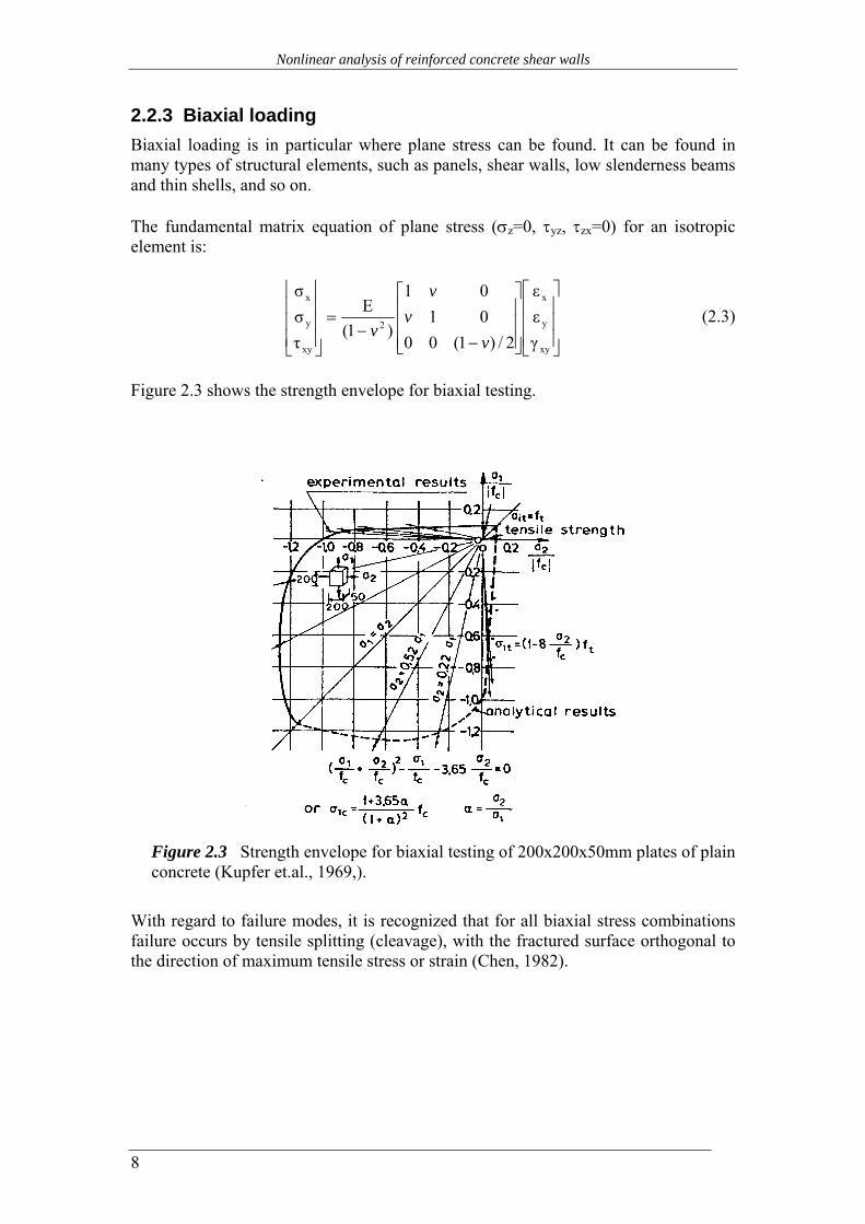
Figure 2.3 shows the strength envelope for biaxial testing.
Figure 2.3 Strength envelope for biaxial testing of 200x200x50mm plates of plain concrete (Kupfer et.al., 1969,).
With regard to failure modes, it is recognized that for all biaxial stress combinations failure occurs by tensile splitting (cleavage), with the fractured surface orthogonal to the direction of maximum tensile stress or strain (Chen, 1982).

Nonlinear analysis of reinforced concrete shear walls
9
2.2.4 Triaxial loading Triaxial state of stress is found in all concrete structures but it is only for certain special structures such as containment vessels, prestressed concrete reactor vessels, offshore platforms, submerged structures and dams, that triaxial loading is actually accounted for in analysis. As these structures fall outside the scope of this work, only a brief description will be made here. The strength of concrete under triaxial loading is a function of the three principal stresses σ1, σ2 and σ3. Depending of the amount of tension present, the failure mode can be quite different. For predominantly tensile stresses failure occurs along a well-defined direction and is characterized by a single localized crack; in this case concrete behaved as a brittle softening material. For predominantly compressive stresses a more ductile behavior is exhibited, characterized by more cracks distributed along a broader failure zone. A graphic reprint of this criterion is shown in Figure 2.4.
Figure 2.4 Failure criterion, presented in the three-dimensional principal stress state (Ottosen, 1977).
2.2.5 Reinforcing steel bars In Figure 2.5 are given stress (σs)-strain (εs) diagrams for various grades of steel, subjected to monotonic tensile loading. It is clear from these diagrams that as the strength of steel increases, its ultimate deformation decreases, a tendency similar (but more marked) than that found for plain concrete. Moreover, the ratio of maximum stress (fu) to yield stress (fy) increases with the steel grade, that is the influence of strain hardening is larger in high strength steel, for which the threshold of the hardening branch is close to the yield strain than in low strength steel.

Nonlinear analysis of reinforced concrete shear walls
10
εs(%)
Figure 2.5 Stress-strain diagrams for steel bars of various grades (see Penelis & Kappos, 1997).
2.3 Ductility The displacement ductility factor is often defined mathematically as the ratio of deformation at a given response level to deformation at yield response. Thus in relation to base shear - displacement relationship of Figure 2.6, response is idealized by an equivalent bilinear curve by extrapolating the elastic response up to the strength Sy to obtain the yield displacement Δy. The ultimate displacement ductility factor is defined as the ultimate displacement divided by the yield displacement or μ=Δu/Δy see Figure 2.6. S: Base shear force Sy Δ: Displacement
Figure 2.6 Definition of the displacement ductility factor (Penelis & Kappos, 1997).
fy fu
Δu Δy
yΔΔμ =

Nonlinear analysis of reinforced concrete shear walls
11
In Paulay and Priestley (1992) it is possible to satisfy the performance criteria of the ultimate limit state and collapse limit state, by any one of following three distinct design approaches, related to the level of ductility permitted of the structure. An illustration of these approaches is shown in Figure 2.7, where strength SE, required to resist earthquake-induced forces and structural displacements Δ at the development at different levels of strength are related to each other.
Figure 2.7 Relationship between strength and ductility (Paulay and Priestley, 1992)
a) Elastic response. Because of their great importance, certain buildings have to
remain essentially elastic under seismic loading. Other structures of lesser importance may nevertheless possess a level of inherent strength such that elastic response is assumed. The idealized response of such a structure is shown in Figure 2.7 by the bilinear strength-displacement path OAA′. The maximum displacement Δme is very close to the displacement of the ideal elastic structure Δe
and the displacement of the real structure Δye at the onset of yielding. b) Ductile response. Most ordinary buildings are designed to resist lateral seismic
forces which are smaller that those that would be developed in a elastically responding structure as Figure 2.7 shows, that inelastic deformations and hence ductility will be required of the structure. These structures can be divided into two groups.
a. Fully Ductile Structures; These are designed to possess the maximum ductility potential that can reasonably be achieved at carefully identified and detailed inelastic regions. The idealized bilinear response of this type of structure is shown in Figure 2.7 by the path OCC′.
b. Structures with Restricted Ductility: Certain structures inherently possess significant strength with respect to lateral forces as a consequence, for example, of the presence of large areas of structural walls.
It should be appreciated that precise limits cannot be set for structures with full and reduced ductility. Figure 2.7 shows approximate values of ductility factors μ, which may be used as guides for the limits of the categories discussed. Although displacement ductility in excess of 8 can be developed in some well-detailed reinforced concrete structures, the associated maximum displacements Δmf are likely

Nonlinear analysis of reinforced concrete shear walls
12
to be beyond limits set by other design criteria, such as structural stability. Elastically responding structures, implying no or negligible ductility demands, represents the other limit (Paulay & Priestley, 1992). From this the capacity design of structures for earthquake resistance has been developed (Paulay & Priestley, 1992). In capacity design distinct elements of the primary lateral force resisting system are chosen and suitably designed and detailed for energy dissipation under severe imposed deformations. The critical regions of these members, often termed plastic hinges, are detailed for inelastic flexural action and shear failure is inhibited by a suitable strength differential. All other structural elements are then protected against actions that could case failure, by providing them with strength greater than that corresponding to development of maximum feasible strength in the potential plastic hinge regions
2.4 Mathematical modelling of concrete and steel
2.4.1 Introduction Many models have been proposed for the nonlinear finite element [FE] analysis of reinforced concrete beams and shear walls under plane stress conditions. These can be classified into linear elastic models, orthotropic models, nonlinear elastic models, plasticity models, endochronic models, fracture mechanics models and micromodels. An overview of these models is available in Chen (1982) and ASCE (1994). In the following the failure criteria of concrete and the flow theory of plasticity will be summarized. More detailed description is given in Chen (1982). The focus is set on those principals because the analytical tools used in this work use plasticity based models for reinforced concrete.
2.4.2 Failure criteria of concrete The strength of concrete under multiaxial stresses is a function of the state of stress and cannot be predicted by limitations of simple tensile, compressive, and shearing stresses independently of each other. In this chapter failure is defined as the ultimate load-carrying capacity of a concrete element. A failure criterion of isotropic materials based upon state of stress must be an invariant function of the state of stress, i.e. independent of the choice of the coordinate system. The function can be presented by the use of principal stress i.e.,
f(σ1,σ2,σ3) = 0 (2.4) The three principal stress can be expressed in terms of the combination of three principal-stress invariants I1, J2 and J3, where I1 is the first invariant of the stress tensor σij and J2, J3 are the second and third invariants of the deviatoric stress tensor sij. Thus replace Eq. (2.4) by,
f(I1,J2,J3) = 0 (2.5) Theses three principal invariants have been used in formulation of various criteria of failure for concrete material.
Nonlinear analysis of reinforced concrete shear walls
13
The hydrostatic axis in the stress space can be defined with the diagonal, d, which has equal distances from the three axes. It follows that the unit vector e along this diagonal is given by
[ ]1113
1=e (2.6)
and every point on the diagonal d is characterized by σ1 = σ2 = σ3 (2.7) i.e., every point on this line corresponds to a hydrostatic stress state, the deviatoric stresses being equal to zero. This diagonal axis is therefore called the hydrostatic axis. The planes perpendicular to d will be called deviatoric planes. The deviatoric plane σ1 + σ2 + σ3 = 0 (2.8) which passes through the origin is called a π plane. The stress point on a π plane represents a pure shear state with no hydrostatic-pressure component. The failure surface in Eq. (2.5) can also be presented be conveniently by f(h,r,θ) = 0, where the variables have been given a geometrical interpretation, see Figure 2.4, There the failure surface is plotted in the coordinate system σ1, σ2 and σ3. The general shape of a failure surface in a three-dimensional stress space can be described by its cross-sectional shapes in the deviatoric planes and its meridians in the meridian planes (see Figure 2.4). The cross sections of the failure surface are the intersection curves between the failure surface and a deviatoric plane, which is perpendicular to the hydrostatic axis with h = constant. The meridians of the failure surface are the intersection curves between the failure surface and a plane (the meridian plane) containing the hydrostatic axis with θ = constant. Concrete failures can be divided into tensile and compressive types. Under tensile and small compressive type of stresses, concrete will fail by a cleavage type of brittle fracture with very little plastic flow before failure. Under high hydrostatic pressure, concrete can yield and flow like a ductile material on the failure or yield surface. Several models have been presented to model the failure surface for each failure tensile or compression or both. They can be classified (see Chen, 1982) into one (i.e. Rankine or Tresca-von Mises), two (i.e. Mohr-Coulomb or Drucker-Prager criterion), three (i.e. Bresler-Pister), four (i.e. Ottosen see Figure 2.4) and five (i.e. William-Warkne) parameter models.
2.4.3 Fundamental concepts of the flow theory of plasticity Plasticity theory provides a mathematical relationship that characterizes the elasto-plastic response of materials as seen in Figure 2.8 after yield point, A. The dependence of yield function on the mean normal stress and the concept of flow rule lead, in general, to an increase in plastic volume under pressure. A yield surface called a loading surface, which combines both perfect plasticity and strain hardening,

Nonlinear analysis of reinforced concrete shear walls
14
is postulated, and an associated flow rule is used for the plastic concrete before fracture.
Figure 2.8 Uniaxial stress-strain curve, pre- and postfailure regime (Chen, 1982).
Figure 2.9 shows a trace of the initial yield surface and the fracture surface in biaxial stress plane. When the state of stress lies within the initial yield surface, the material is assumed to be linear and the linear-elastic equations can be applied. When the material is stressed beyond the initial-yield or elastic-limit surface, a subsequent new yield surface called the loading surface is developed. The new surface replaces the initial yield surface. If the material is unloaded from, and reloaded within, this subsequent loading surface, no additional irrecoverable deformation will occur until this new surface is reached. If straining is continued beyond this surface, further discontinuity and additional irrecoverable deformation results.
Figure 2.9 Loading surfaces of concrete in the biaxial stress plane for a work-hardening-plasticity model (Chen, 1982).
The flow theory of plasticity is normally used to model concrete behaviour in compression but can also be used in tension before cracking. The formulation refers to a rectangular, cartesian coordinate system. Four basic assumptions are made.

Nonlinear analysis of reinforced concrete shear walls
15
The first assumption is that total strains are obtained by adding elastic strains to plastic strains:
pij
eijij εεε += (2.9)
The elastic strains are related to the stresses by Hooke’s law which may be anisotropic
ekl
eijklij εD dd +=σ (2.10)
The plastic part of the deformation is taken to be incompressible, i.e.
0ε pii = (2.11)
The second assumption is that there exists a “loading function” f, which depends upon the state of stress and strain and the history of loading, where f=0 corresponds to the yield condition. Considering hardening materials, f is dependant of the state of stress σij, the plastic strains and the hardening parameter k, i.e.
k),ε,f(σf pijij= (2.12)
Depending on the value of f, different material states can be defined: f < 0 elastic f = 0 plastic f > 0 not admissible The total differential of f in a plastic stage, where f=0 is
kκfε
εfσ
σf f p
ijpij
ijij
dddd∂∂
+∂∂
+∂∂
= (2.13)
Three possible cases of further loading can be defined from Eq (2.13):
0σσf
ijij
<∂∂ d ; f = 0 ; unloading
0σσf
ijij
=∂∂ d ;f = 0 ; neutral loading (2.14)
0σσf
ijij
>∂∂ d ;f = 0 ; loading
The third assumption is concerned with the hardening rule. Several hardening rules have been proposed for use in plastic analysis. Two types of hardening rules are considered here i.e. isotropic hardening and kinematic hardening. The isotropic-hardening rule assumes a uniform expansion of the initial yield surface, and the subsequent yield surfaces can be written as
f(σij,k) = F(σij) - σe(εp) = 0 (2.15)

Nonlinear analysis of reinforced concrete shear walls
16
in which εp, called effective plastic strain, depends on the plastic strain history and σe, called the effective stress, is the uniaxial yield stress. The concept of effective stress and effective strain makes it possible to extrapolate from a simple uniaxial tension or compression test into the multidimensional situation. The effective stress is usually defined as the same function of the stresses that governs yielding, i.e., as the loading function F(σij) = σe(εp) which maps the multiaxial stress state onto equivalent scalar functions εp defined either by the plastic work Wp hypothesis or by the accumulated plastic strain hypothesis as
dWp = σedεp or dεp = pij
pij εε dd (2.16)
The kinematic-hardening rule considers the Bauschinger effect and the development of anisotropy due to plastic deformation. The simplest version for determining the hardening parameter αij is to assume a linear dependence of dαij and p
ijεd . This is known as Prager’s hardening rule which has the form:
pijij εcα dd = (2.17)
where c is the work-hardening constant, characteristic for a given material. and the loading function has the general form
0σ)αF(σ)ε,f(σ 0ijijpijij =−−= (2.18)
σ2 σ2 Initial yield surface Initial yield surface Subsequent yield surface
(a) Isotropic work hardening (b) Kinematic hardening
Figure 2.10 Hardening rule a) isotropic work hardening and b) kinematic hardening.
The fourth assumption is that for an idealized plastic material it is possible to define a plastic potential function k),ε,g(σ p
ijij . The gradient of the potential surface defines the direction of the plastic-strain increment, while the length is determined by the loading parameter dλ. The flow rule is associated if the plastic potential has the same shape as the yield condition k),ε,g(σ p
ijij = k),ε,f(σ pijij , than
Subsequent yield surface
σ1σ1
Nonlinear analysis of reinforced concrete shear walls
17
ij
pij σ
fε∂∂
λ= dd (2.19)
To derive constitutive equation, we substitute Hook’s law
)εε(D pklkl
eijklij ddd +=σ (2.20)
into the consistency condition (2.13) using the flow rule (2.19), and solve for the scalar function dλ. Substitution of dλ so obtained into (2.20) gives the constitutive equations of the elastoplastic material,
klpijkl
eijklkl
epijklij ε)DD(εD ddd +==σ (2.21)
which relates increments of stress uniquely with corresponding increments of strain. Using engineering stresses and strains, and assuming that (2.21) is also valid for finite increments, the incremental stress-strain relation can be written in a matrix form
△σ =Dep△ε =(De-Dp)△ε (2.22)
2.5 Finite element approximations
2.5.1 Formulation of the flow theory of plasticity
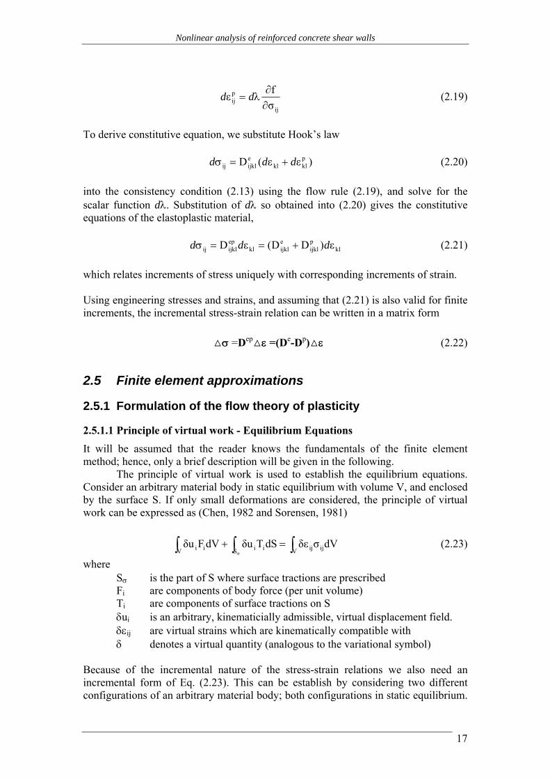
2.5.1.1 Principle of virtual work - Equilibrium Equations It will be assumed that the reader knows the fundamentals of the finite element method; hence, only a brief description will be given in the following. The principle of virtual work is used to establish the equilibrium equations. Consider an arbitrary material body in static equilibrium with volume V, and enclosed by the surface S. If only small deformations are considered, the principle of virtual work can be expressed as (Chen, 1982 and Sorensen, 1981)
∫∫ ∫ =+
V ijijiV S iii dVσδεdSTδudVFδuσ
(2.23)
where Sσ is the part of S where surface tractions are prescribed Fi are components of body force (per unit volume) Ti are components of surface tractions on S δui is an arbitrary, kinematicially admissible, virtual displacement field. δεij are virtual strains which are kinematically compatible with δ denotes a virtual quantity (analogous to the variational symbol) Because of the incremental nature of the stress-strain relations we also need an incremental form of Eq. (2.23). This can be establish by considering two different configurations of an arbitrary material body; both configurations in static equilibrium.

Nonlinear analysis of reinforced concrete shear walls
18
It is assumed that the configurations are close to each other (small increments). The incremental form of the principle of virtual work is given by
∫∫ ∫ σΔΔ=ΔΔ+ΔΔV ijijiV S iii dV)εδ(dST)uδ(dVF)uδ(
σ
(2.24)
Since only small deformations are considered the incremental quantities are obtained simply as differences between two adjacent configurations.
2.5.1.2 Implementation of the flow theory of plasticity Let us consider an assemblage of finite elements. The displacement field within element no. e is defined by
ue = Neve (2.25) in which ve contains nodal displacements Ne is a matrix of assumed interpolation polynomials
Ue contains the displacement components at an arbitrary point within the element.
The strains at a point within the element can be expressed as
εe = Beve (2.26) where the matrix Be contains the derivatives of Ne with respect to the coordinate axes. Eq. (2.23) and (2.24) can be rewritten in matrix form as
0dVδdSδdVδV
T
S
T
V
T
σ
=−+ ∫∫∫ σεTuFu (2.27)
0dVΔδΔdSΔ)δ(ΔdVΔ)δ(Δ
V
T
S
T
V
T
σ
=−+ ∫∫∫ σεTuFu (2.28)
Equilibrium of the finite element assemblage can be obtained by combining Eq. (2.25), (2.26) and (2.27) for all N elements
0dV)dVdVδN
1e V S Ve
Tee
Tee
Te
Te
e σ e
=⎥⎥⎦
⎤
⎢⎢⎣
⎡
⎟⎟⎠
⎞⎜⎜⎝
⎛−+∑ ∫ ∫ ∫
=
σBTNFNv (2.29)
The element nodal displacements ve are related to the system displacements vector r by the connectivity matrix
ve = aer (2.30) Eq. (2.29) can be rewritten as

Nonlinear analysis of reinforced concrete shear walls
19
( )[ ] 0δN
1eσ
Tee
Te
Te
=−∑=
SaPar (2.31)
Here is
Pe = Pbe + Pse (2.32) i.e. the sum of all external load on the element (body and surface loads)
∫=eV
eTebe dVFNP (2.33)
∫
σ
=eS
eTese dSTNP (2.34)
The incremental forces can be found from
∫=σ
e
e
Ve
Te dVσBS (2.35)
Eq. (2.31) must hold for arbitrary virtual displacements δr; hence, the equilibrium equations for the assemblage of elements can be written
R - Rσ = 0 (2.36) in which
∑=
=N
1ee
Te RaR (2.37)
∑=
σσ =N
1e
Te eSaR (2.38)
Since only small deformations are considered, Be of Eq.(2.26) and Pe of Eq. (2.32) are independent of state of deformation. The stresses σe of Eq. (2.35) depends on the deformations; consequently, the equilibrium equations (2.36) are nonlinear in terms of displacements. The incremental form is therefore needed to find a solution that satisfies Eq. (2.36)
0dV)ΔdSΔdVΔ)δ(ΔN
1e V S Ve
Tee
Tee
Te
Te
e eσ e
=⎥⎥
⎦
⎤
⎢⎢
⎣
⎡
⎟⎟
⎠
⎞
⎜⎜
⎝
⎛−+∑ ∫ ∫ ∫
=
σBTNFNv (2.39)
The incremental stress-strain relation of Eq (2.22) is substituted into Eq. (2.39) and by use of Eq. (2.26) and (2.30) the following incremental equilibrium equations are obtained:
Nonlinear analysis of reinforced concrete shear walls
20
0Δ)dVdSdVΔN
1e V S Vee
epe
Te
Tee
Te
Tee
Te
Te
e eσ e
=⎟⎟
⎠
⎞
⎜⎜
⎝
⎛−+∑ ∫ ∫ ∫
=
raBDBaTNaFNa (2.40)
Further we introduce:
∑ ∫ ∫= ⎥
⎥
⎦
⎤
⎢⎢
⎣
⎡
⎟⎟
⎠
⎞
⎜⎜
⎝
⎛Δ+Δ=Δ
σ
N
1e V Se
Tee
Te
e e
dSdV TNFNR (2.41)
( )∑ ∫=
=N
1e Vee
epe
Td
Te
e
dVaBDBaK (2.42)
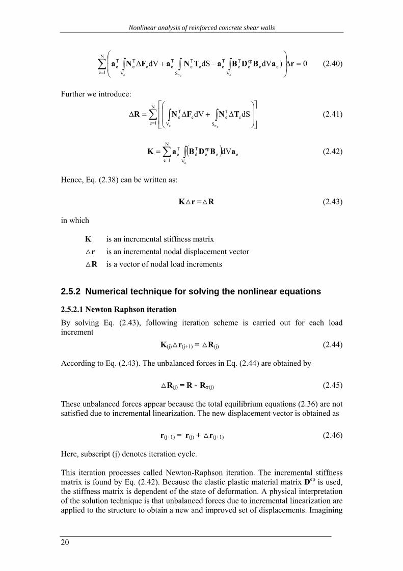
Hence, Eq. (2.38) can be written as:
K△r =△R (2.43) in which
K is an incremental stiffness matrix △r is an incremental nodal displacement vector △R is a vector of nodal load increments
2.5.2 Numerical technique for solving the nonlinear equations
2.5.2.1 Newton Raphson iteration By solving Eq. (2.43), following iteration scheme is carried out for each load increment
K(j)△r(j+1) = △R(j) (2.44) According to Eq. (2.43). The unbalanced forces in Eq. (2.44) are obtained by
△R(j) = R - Rσ(j) (2.45) These unbalanced forces appear because the total equilibrium equations (2.36) are not satisfied due to incremental linearization. The new displacement vector is obtained as
r(j+1) = r(j) + △r(j+1) (2.46) Here, subscript (j) denotes iteration cycle. This iteration processes called Newton-Raphson iteration. The incremental stiffness matrix is found by Eq. (2.42). Because the elastic plastic material matrix Dep is used, the stiffness matrix is dependent of the state of deformation. A physical interpretation of the solution technique is that unbalanced forces due to incremental linearization are applied to the structure to obtain a new and improved set of displacements. Imagining

Nonlinear analysis of reinforced concrete shear walls
21
the load and displacement vectors as single components, the process can be illustrated as shown in Figure 2.11.
Figure 2.11 Incremental and iterative solution illustrated as a load deflection relationship.
The iteration process implies the following computational steps for each iteration cycle
i) Computation of Rσ from Eq. (2.35) and (2.38) ii) Computation of incremental stiffness matrix K iii) Triangularization of K
These three steps have to be carried out if the stiffness is updated at each iteration cycle. Other iteration algorithms are also known, such as the arc-length technique see ANSYS (1998) or COSMOS (1996).
2.5.2.2 Load incrementation and convergence criteria Due to the incremental linearization, the unbalanced forces will increase if the load increments are increased. This results in a great number of iterations to re-establish equilibrium in the system. The choice of load increment size is important for the economy of a nonlinear analysis. A convergence criterion for termination of the equilibrium iteration process is also required in computer programs. A criterion for termination of the equilibrium process is also required. Computer programs usually use a criterion based on a force or displacement. For displacement it is:
ref,k
k
rrΔ
=ε (2.47)
△rk is a characteristic incremental displacement component. rk,ref is the total value of the same displacement component.
Rσ(1) Rσ(2) Rσ(3)r(1)
r(2) r(3)
△r(2)
△r(3)
K(0)
K(1) K(2)
△R
△R
R
R
r
△R(2)

Nonlinear analysis of reinforced concrete shear walls
22
The following criterion is often used
γ≤ε (2.48) The iteration process is terminated when the inequality of Eq.(2.48) is satisfied. The value of γ are usually in the range from 10-2 to 10-3. For slowly converging systems it is also necessary to terminate the process after a prescribed maximum number of iterations to reduce the effect of possible input accidents.
2.6 ANSYS – Reinforced Concrete Solid The solid element in ANSYS (1998) named SOLID65, can be used for three dimensional modelling of solids with or without reinforcing bars (rebars). Eight nodes having three degrees of freedom at each node define the element: translations in the nodal x, y, and z directions. Up to three different rebar specifications may be defined. The most important aspect of this element is the treatment of nonlinear material properties. The solid (e.g. concrete) is capable of cracking (in three orthogonal directions), crushing, deform plastically, and creep. The rebars are capable of tension and compression, but not shear. They are also capable of deform plastically and creep. The geometry, node locations, and the coordinate system for this element are shown in Figure 2.12. The volume ratio is defined as the rebar volume divided by the total element volume. The orientation is defined by two angles (in degrees) from the element coordinate system.
Figure 2.12 The concrete element in ANSYS, SOLID 65.
The following assumptions and restrictions are made:
1. Cracking is permitted in three orthogonal directions at each integration point. If cracking occurs at an integration point, the cracking is modelled though an adjustment of material properties (i.e. by changing the element stiffness matrixes) which effectively treats the cracking as a “smeared ” cracks. According to Chen (1982) the smeared-cracking model is considered to be better then discrete-cracking model or fracture-mechanics model.
2. The concrete material is assumed to be initially isotropic.

Nonlinear analysis of reinforced concrete shear walls
23
3. Whenever the reinforcement capability of the element is used, the reinforcement is assumed to be “smeared” throughout the element.
4. If the concrete at an integration point fails in uniaxial, biaxial, or triaxial compression, the concrete is assumed to crush at that point. Crushing is defined as the complete deterioration of the structural integrity of the concrete (e.g. concrete spalling).
5. In addition to cracking and crushing, the concrete may also undergo plasticity, with the Drucker-Prager failure surface being most commonly used. In this case, the plasticity is done before the cracking and crushing checks.
The concrete materials data, such as the shear transfer coefficients, tensile stresses, and compressive stresses are input in the data table see Table 2.1. Typical shear transfer coefficients range from 0.0 to 1.0, with 0.0 representing a smooth crack (complete loss of shear transfer) and 1.0 representing a rough crack (no loss of shear transfer). This specification may be made for both the closed and open crack.
Table 2.1. Data to be entered in ANSYS model. Constant Meaning
Label
1 Shear transfer coefficients for an open crack βt 2 Shear transfer coefficients for a closed crack βc 3 Uniaxial tensile cracking stress (positive) ft 4 Uniaxial crushing stress (positive) fc 5 Biaxial crushing stress (positive) fcb 6 Ambient hydrostatic stress state for use with constants 7 and 8 σh 7 Biaxial crushing stress (positive) under the ambient hydrostatic
state (constant 6) f1
8 Uniaxial crushing stress (positive) under the ambient hydrostatic stress state (constant 6).
f2
9 Stiffness multiplier for cracked tensile condition. Tc The failure surface is expressed in terms of principal stresses and five input parameters ft, fc, fcb, f1 and f2, but the failure surface can be specified with a minimum of two constants, ft and fc. The other three constants can be calculated as default to William and Warnke (1975) i.e.
fcb = 1.2 fc (2.49)
f1 =1.45 fc (2.50)
f2 = 1.725 fc (2.51) The stiffness multiplier Tc in Table 2.1, which represents the tension stiffness effect, has a default value of 0.6 see Figure 2.13. When using the rate independent plasticity theory in the ANSYS program there are three aspects that have to be determined, that is the yield criterion, flow rule and the hardening rule.

Nonlinear analysis of reinforced concrete shear walls
24
1 εck 6 εck
Figure 2.13 Strength of cracked condition (ANSYS, 1998).
2.7 COSMOS/M - A bounding surface model for concrete The concrete model is a three-dimensional, rate-independent model with a bounding surface sees Chen and Buyukozturk (1985) and COSMOS/M user manual (1996). The model adopts a scalar representation of the damage related to the strain and stress states of the material. The bounding surface in the stress space shrinks uniformly as the damage due to strain softening and/or tension cracks accumulates. The material parameters depend on the damage level, the hydrostatic pressure, and the distance between the current stress point and the bounding surface. The damage coefficient is representing the damage happens to the material due to strain hardening or softening. The damage coefficient value is always positive and the magnitude of it in conjunction with the hydrostatic pressure represents the damage due to compression and tension cracking. For instance, the damage happens in a uniaxial compression test at the ultimate strength is normalized to be one and for uniaxial tension test to be approximately 0.2. The damage is obtained by integrating the incremental damage coefficient that depends on the plastic strain and the distance from the current stress state and the bounding surface. The model is defined by two material parameters, which are:
1. fc = the concrete ultimate strength 2. εu = the ultimate strain
The parameters are temperature independent. Moreover the model should be used with conjunction with small strain formulation. The model has a compression strain hardening and softening capabilities. However in the tension stresses, the model behaves as a nonlinear strain hardening material until it reaches the tension strength and starts to behave as a perfect plastic material. The maximum tensile strength for uniaxial test is considered as:
ft = 0.17 fc (2.52)
ε
σ
ft
Tcft
Ec

Nonlinear analysis of reinforced concrete shear walls
25
3. Nonlinear analysis of laboratory tested RC elements
3.1 Introduction
3.1.1 Background The objective is to find an analytical tool, which gives good correlation to experimental results for reinforced concrete elements. Two tested RC beams and two tested RC walls are analysed. The RC beams were laboratory tested by Bresler & Scordelis (1964) and the RC walls by Barda (1972). One RC beam is analysed with three different programs see chapter 3.1.3 and chapter 3.2.1. As a result, one program is used in subsequent analysis. The analytical programs are ANSYS and COSMOS/M, which are available at the faculty of Engineering of the University of Iceland. In additional to these programs, the program PCFEARC is also tested for comparison. The last program has some limitations.
3.1.2 Analytical modelling steps and tools Before doing the nonlinear analysis it is necessary to consider the following steps, namely. (1) The geometry of the structure. (2) Loads. (3) Material modelling of concrete, i.e. elastic - plastic behavior of concrete in compression and tension, failure- and yield criteria, flow rule and hardening rule, crushing/cracking and aggregate interlock in open crack. (4) Material modelling of reinforcement i.e. elastic-plastic and hardening. (5) Interactive between concrete and reinforcement i.e. with or without bond slip, tension stiffening or dowel effects. (6) Finite element approximations. (7) Numerical technique for solving the nonlinear equations i.e. Newton-Rapson and convergence criteria. (8) Boundary condition. Three FE models were tested i.e. ANSYS, COSMOS/M and PCFEARC. The finite element model created in ANSYS is three dimensional. The concrete is modelled with the SOLID65 element, see chapter 2.6. The mathematical modelling of the materials is based on the flow theory of plasticity in a very simple form. Simple models in compression are chosen to provide an efficient and inexpensive numerical tool, and may be justified by the fact that tensile cracking and related phenomena often give the dominating contribution to the overall nonlinear behavior of a reinforced concrete member. The plasticity model for concrete and steel is based on the flow theory of plasticity (see chapter 2.4) i.e. Von Mises yield criterion, isotropic hardening and associated flow rule. In our model time dependent deformations are not considered. Shear retention factors in Table 2.1 which present the aggregate interlock contribution is taken as 1.0 for closed crack (βc) and 0.1 for open crack (βt), which is according to Hemmaty (1992,1998). He investigated the shear factors by parametric study. The failure surface for concrete (see chapter 2.6) is specified with the two constants, ft and fc. The default values are used for all other constants. The finite element model created in COSMOS/M is two dimensional see chapter 2.7. Concrete is modelled with the shell element PLANE2D and the reinforced steel bars are modelled with the line element TRUSS2D element. The steel and the concrete are assumed to be fully bonded at node points in the model. The concrete can undergo plasticity in compression and tension but no cracking occur in tension. Effects of

Nonlinear analysis of reinforced concrete shear walls
26
aggregate interlock in open cracks are included as damage. Furthermore, yielding and hardening of reinforcement steel is included. The failure surface for concrete is specified with the two constants, fc and εu. The finite element model created in PCFEARC (Sorensen, 1981 and Kvarme, 1990) is two dimensional. The computer program takes into account material nonlinearites like inelastic behavior in compression and cracking in tension of concrete. Effects of aggregate interlock in open cracks are included. Furthermore, yielding and hardening of reinforcement steel is included. The flow theory of plasticity as described in chapter 2.4, is used to model the concrete behavior in biaxial compression; i.e. the von Mises yield function with isotropic hardening is used. Concrete is modelled with an isoparametric quadriateral element and the reinforced steel bars are modelled with line element, see Sorensen (1981) for further detail. The steel and the concrete are assumed to be fully bonded at node points in the model. The capacity of the computer program is around 90 elements, for larger problems the working domain has to be expanded. The Newton-Rapson iterations technique was used in all programs see chapter 2.5.2 and programs were tested with various load step size and various convergence criteria.
3.1.3 Failure mechanism for the analysed RC elements In Chen (1982) is a detailed description of causes of failure in RC beams. Paulay and Priestley (1992) have summered up the failure mechanism for walls. The failure mechanisms for squat walls are shown in Figure 3.1. They are, diagonal tension failure (see Fig. 3.1 (a) & (b)), diagonal compression failure (see Fig. 3.1 (c) &(d)) and phenomenon of sliding shear (see Fig 3.1 (e)).
Figure 3.1 Shear failure modes in squat walls (Paulay and Priestley, 1992).

Nonlinear analysis of reinforced concrete shear walls
27
3.2 RC beams
3.2.1 Description of laboratory test In Bresler and Scordelis (1964) the laboratory tests of the beams are described. A series of twelve beams was tested. All parameters that are used in the following FE analyse can be found there. Two tested beams are considered. The first beam has no shear reinforcement (specimen OA1) and fails with diagonal tension failure. The second beam has shear reinforcement (specimen A1) and fails with shear compression failure. Beams OA1 and A1 are the same size. The beam dimensions are as follows (also see Figure 3.2). Span length (L) = 3660 mm Width (b) = 305 mm Total depth (h) = 552 mm Effective depth (d) = 458 mm Because the beams are symmetrical with respect to the centreline, only half of the beams are modelled. The beams are simple supported and loaded with single force (P) gradually increased at the middle. P ℄
Figure (a) P ℄
Figure (b) Figure 3.2 Test specimen a) specimen OA1 – no shear reinforcement and b) specimen A1 - with shear reinforcement.
L/2 = 1830 mm
230 mm
: :
b
h d
x
z
y
. .
L/2 = 1830 mm
230 mm
: :
b
h d
x
z
y

Nonlinear analysis of reinforced concrete shear walls
28
Specimen OA1 has only tension reinforcement while specimen A1 has tension, compression reinforcement and stirrups see Table 3.1.
Table 3.1 Reinforcement in beam specimen OA1 and A1.
Beam Reinforcement Number of bars/ stirrups
Area of each bar (mm2)
Total area of steel, As
(mm2)
As/Ac
A1 & OA1 Tension steel 4 650 2.600 1.80 % A1 Compression steel 2 151.5 303 0.18 % A1 Stirrups in A1 c/c 210mm 23 28.3 1.300 0.10 %
The load producing initial cracking (Pcr), diagonal tension crack (Pdcr) and the ultimate test load (Pu) are given in Table 3.2.
Table 3.2 Cracking load, failure and ultimate load for modeled beams.
Failure Beam with no shear reinforcement OA1
Beam with shear reinforcement A1
Load producing initial crack (Pcr/2) 35-40 kN 35-40 kN Load producing initial diagonal tension crack (Pdcr/2)
133.5 kN
133.5 kN
Ultimate test load (Pu/2) 167.0 kN 233.5 kN In the experiments of the beam OA1 it was observed that the beam failed by a rapid diagonal tension failure mechanism. The beam failed shortly after the formation of the “critical diagonal tension crack”. The failures observed as a result of longitudinal splitting in the compression zone near the load point, and also by horizontal splitting along the tensile reinforcement near the end of the beam. Failures were brittle; the critical cracks formed at a load of approximately 80 % of the ultimate load. Although the beam carried some additional load after the formation of the critical crack, the deterioration was rapid as evidenced principally by opening of the crack. In the experiments of the beam A1 failure took place at loads substantially greater than the load at which the initial diagonal tension crack occurred. The diagonal tension cracks formed at approximately 60 percent of the ultimate load. Additional load cased further diagonal cracking but caused no visible signs of distress. Failures developed without extensive propagation of flexural cracks in the center portion of the span indicating that the mechanism of failure was of shear compression. Final failures occurred by splitting in the compression zone but without splitting along the tension reinforcement, which was characteristic of beams without shear reinforcement.

Nonlinear analysis of reinforced concrete shear walls
29
3.2.2 FE-analysis of beam without shear reinforcement OA1 The FE model from ANSYS is shown in Figure 3.3, the element size is similar in the other FE programs tested.
Figure 3.3 Beam without shear reinforcement finite element idealization used in ANSYS.
The material constants used in the nonlinear analysis are listed in Table 3.3.
Table 3.3 Beam material parameters used in computer models.
Nr Parameter Numerical value
ANSYS COSMOS PCFEARC
1 Secant modulus of elasticity,(Ec) 23.9 GPa 23.9 GPa 23.9 GPa 2 Uniaxial ultimate compression strength (fc) 22.6 MPa 22.6 MPa 22.6 MPa 3 Secant modulus of plasticity (ET) 1640 MPa - 1640 MPa 4 Uniaxial yield strength for concrete 0.8 x fc - 0.8 x fc 5 Uniaxial tensile strength (ft) 3.0 MPa - 3.0 MPa 6 Ultimate strain for concrete (εu) 3.5 ‰ - 3.5 ‰ 7 Shear transfer coefficient for an open crack (βt) 0.1 - 0.1 8 Shear transfer coefficient for a closed crack (βc) 1.0 - 1.0 9 Multiplier for tensile stress relaxation (Tc) 0.6 - - 10 Poisson‘s ratio for concrete (ν) 0.2 0.2 0.2 11 Modulus of elasticity for steel (Es) 206 GPa 206 GPa 206 GPa 12 Modulus of plasticity for steel (Ep) 9 GPa 9 GPa 9 GPa 13 Yield point of steel reinforcement (fy) 555 MPa 555 MPa 555 MPa 17 Ultimate strain for tension steel (εsu) 13 ‰ 13 ‰ 13 ‰ 14 Poisson’s ratio for steel (vs) 0.3 0.3 0.3 15 Weight of concrete 24 kN/m3 24 kN/m3 -
The total weight of the beam is 15.6 kN.

Nonlinear analysis of reinforced concrete shear walls
30
Table 3.4 Finite element model of OA1.
Nr Finite element model
ANSYS COSMOS PCFEARC
1 Dimension of model 3D 2D 2D 2 Total number of concrete elements 144 72 42 3 Total number of reinforcement elements 48 24 7 4 Cracking and crushing of concrete Yes No Yes 6 Number of load steps 50 50 8 7 Gravity load Yes Yes No 10 Convergence criteria Displacement L2
norm, γ = 0.001 Default to program
Displacement norm, γ = 0.01
Load (P) is applied slowly to the top of the beam, in the 2D models the load is applied on one node on the top but in the ANSYS 3D model the load is applied on 3 nodes, that is 50% in the middle (on node) and 25% sideways (two nodes). In ANSYS and COSMOS an automatic load step size option was used or total number of 40-50 load increments. In PCFEARC only 8 load increments were used, because the total number of load increments that the program can handle is nine. Boundary conditions are shown in Figure 3.3 where the supported end is free in x-direction (longitudinal) but fixed in y-direction (vertical). Also where the beam is cut into half all nodes are fixed in x and z-direction. Figure 3.4 shows stress-strain relation model for concrete and steel used in analysis of the OA1 beam.
0
250
500
750
1000
0 2 4 6 8 10 12 14 16Steel strain [%]
Stee
l str
ess
[MPa
]
Experim. - tension steelBilinear model - tension steelExperim. - compr. steelBilinear - compr./stirrupsExperim. - Stirrups
Ep
Es
Figure (a)

Nonlinear analysis of reinforced concrete shear walls
31
-4
0
4
8
12
16
20
24
-1 0 1 2 3 4
Concrete strain [‰]
Con
cret
e st
ress
[MPa
]
Bilinear model
Uniaxial concrete strength
Ec
ET
Figure (b)
Figure 3.4 Stress-strain relation used for investigation of OA1 a) reinforcement and b) concrete.
Figure 3.5(a) shows the comparison of the deflection-load curves for FE models and experimental results for beam OA1. There it can be observed that the ANSYS model and PCFEARC simulate the beam behavior very well in comparison with the experiment. In the experiment the initial cracks start to form at the load of 40 kN. In the ANSYS and PCFEARC models initial cracking starts at same load level. Figure 3.5(b) shows the highest steel stress (at the middle) as a function of load for the FE models. Steel stresses are very similar in ANSYS and PCFEARC but the COSMOS, stresses are quite different.

Nonlinear analysis of reinforced concrete shear walls
32
Figure (a)
Figure (b)
Figure 3.5 Comparison of programs used in modelling beam OA1 without shear reinforcement a) load-deflection curves in the middle of the beam and b) steel stresses-load curves for tension steel.
In ANSYS cracking is shown with a circle outline in the plane of the crack, and crushing is shown with an octahedron outline. If the crack has opened and then closed, the circle outline will have an X though it. Each integration point can crack in up to three different planes. The first crack at an integration point is shown with a red
0
50
100
150
200
250
0 2 4 6 8 10 12 14
Deflection [mm]
Load
[kN
]
Linear modelPCFEARC modelExperimentCOSMOS modelANSYS model
0
50
100
150
200
250
300
350
400
450
0 25 50 75 100 125 150 175 200 225 250
Load [kN]
Stee
l str
ess
[Mpa
]
ANSYS model
PCFEARC model
COSMOS model
Linear model

Nonlinear analysis of reinforced concrete shear walls
33
circle outline, the second crack with a green outline, and the third crack with a blue outline. By comparing the computed crack pattern in ANSYS with the experiment at failure load, Pcr, it can be seen that the computed crack patterns strongly indicate diagonal tension failure in the concrete. At this load level the reinforcement and the concrete have not yielded, see Figure 3.5 (b). Table 3.5 shows comparison between the experiment, theory and the FE models. The difference in the deflection is very low except for the EC2-value. The difference in the ultimate load is bigger i.e. the COSMOS value is far bigger than the others.
Table 3.5 Comparison between the experiment, theory and FE models.
Experi-ment
TheoryEC2*)
ANSYS COS-MOS
PC- FEARC
Ultimate load, Pu/2 [kN] 167 174 166.3 250 170 Initial cracking load, Pcr/2 [kN] 35 32.1 36.8 no crack 35 Deflection at Pdcr/2 = 133.5kN [mm] 5.1 7.7 5.3 5.2 5.3
*) Calculated value according to formulas from EC2 and O’Brien and Dixon (1995, pp. 240-274). Crack patterns at ultimate load from experiment and the ANSYS analysis are shown in Figure 3.6 and Figure 3.7. The crack pattern is similar. The secondary cracking that can be observed from the computed crack pattern close to the reinforcement bars may reflect some bond slip effects, since the secondary cracking is nearly parallel to the reinforcement bars.
Figure 3.6 Crack pattern in specimen OA1 at ultimate load (Bresler & Scordelis (1964).

Nonlinear analysis of reinforced concrete shear walls
34
Figure (a)
Figure (b)
Figure (c)
Figure 3.7 Cracking in beam at ultimate load a) first crack, b) second crack and c) third crack.
At this point it is decided to reject COSMOS, because of its limitiations in modeling cracking and steel stresses. If is obvious from the comparison that tension cracking of concrete plays the most important role among the nonlinear effects of concrete in the beam while a relatively simple approximation of the concrete behavior in compression seems to be enough. The PCFEARC program is based on similar theory as ANSYS but the program is limited to 90 elements and 9 iterations, which is insufficient for larger models. The PCFEARC model can be fixed enlarging vector and matrix dimensions in program. The source code is not available and it is not possible to use it for shear walls so it will not be used further. In the remaining it will therefore only be focused on the ANSYS program. Before going further it is useful to investigate the accuracy of the ANSYS model and see how sensitive the results are for changes in the input parameters. Some of the results of this testing is shown in Table 3.6.

Nonlinear analysis of reinforced concrete shear walls
35
Table 3.6 Parametric study of the OA1 beam in ANSYS.
Run Changes made from model OA1 Results/ effects
Conclusion
1 Doubling the number of load steps No effects, same results.
Use 4 kN
2 Changing convergence tolerance γ to 0.01 or 0.001
No effects, same results.
Use γ=0.001
3 Changing hardening rule of concrete from bilinear to Drucker Prager with; Cohesion value, c =5.83 Angle of internal friction, θ = 35.5 Dilatancy angle, ϕ = 35.5
Convergence problem.
Stopped at P/2 =122 kN
Have to be studied further.
4 Changing billinar compression model; use ε = 4.0 ‰ instead of 3.5 ‰ and ET = 1387 MPa
Ultimate load 200 kN.
Use ε = 3.5 ‰
*) The Drucker Prager parameters are calculated with formulas from Chen (1982) p.345. Instead of using isotopic or kinematic hardening rule it is also common to use the Drucker-Prager model that allows no hardening and corresponds to a perfectly elastic-plastic material. When the Drucker-Prager model is used, the amount of dilatancy (the increase in material volume due to yielding) can be controlled with the dilatancy angle. If the dilatancy angle is equal to the friction angle, the flow rule is associative. If the dilatancy angle is zero (or less then the friction angle), there is no (or less of an) increase in material volume when yielding and the flow rule is nonassociated. It was also tested to use kinematic hardening instead of isotropic hardening and the results were the same as expected from monotonic loading. In all the FE models perfect bond is assumed. Hemmety (1992) has studied the effects of the perfect and imperfect bond assumptions. He modelled in ANSYS reinforced concrete joint and tested a model with perfect bond and a model with bond slip. He compared the results to laboratory test of the same joint. The failure moment of the specimen was up to 9 % over estimated in the model with the perfect bond. He concluded that in many structural applications it might be acceptable up to this accuracy to model the structure with perfect bond assumption. As seen in the model of the beam this deflection-load curve follow the experiment curve very well so it is concluded that the need for modelling the bond slip is negligible. To model the bond slip behavior between concrete and steel Hemmety (1992, 1998) and Huyse et. al. (1994) uses the nonlinear force-deflection element in ANSYS. This is a unidirectional spring element with a nonlinear generalized force-deflection capability. Furthermore it is worth noting that the test in laboratory is only made once and no bonds or standard deviation of the results are shown. It is likely that repeated tests will have some variations.

Nonlinear analysis of reinforced concrete shear walls
36
3.2.3 FE-analysis of beam with shear reinforcement A1 This beam A1 is identical to OA1 except it has in addition shear reinforcement, compression steel and higher concrete strength, see chapter 3.2.1 and Figure 3.2 (b). Only FE analysis in ANSYS will be considered. The material constants used in the nonlinear analysis of A1 beam are listed in Table 3.7.
Table 3.7 Material parameters for beam specimen A1 used in FE model.
Nr Parameter ANSYS
1 Secant modulus of elasticity, (Ec) 27,000 MPa 2 Uniaxial ultimate compression strength (fc) 24.1 MPa 3 Secant modulus of plasticity (ET) 1,723 MPa 4 Uniaxial yield strength for concrete 0.8 x fc 5 Uniaxial tensile strength (ft) 3.0 MPa 6 Ultimate strain for concrete (εu) 3.5 ‰ 7 Shear transfer coefficient for an open crack (βt) 0.1 8 Shear transfer coefficient for a closed crack (βc) 1.0 9 Multiplier for amount of tensile stress relaxation (Tc) 0.6 10 Poisson‘s ratio for concrete (ν) 0.2 11 Poisson‘s ratio for steel 0.3 12 Modulus of elasticity for steel (Es) 206,000 MPa 13 Modulus of plasticity for tension steel (Ep) 9,000 MPa 14 Yield point of tension steel reinforcement (fy) 555 MPa 15 Modulus of plasticity for comp. steel and stirrups (Ep) 1,000 MPa 16 Yield point of comp. steel and stirrups (fy) 345 MPa 17 Ultimate strain for tension steel (εsu) 13 ‰ 18 Ultimate strain for comp. steel and stirrups (εsu) 16 ‰ 19 Weight of steel 77 kN/m3 20 Weight of concrete 24 kN/m3
The stress-strain curves used for concrete and steel material for beam A1 are similar to those in Figure 3.4 used for the OA1 beam. Finite element model (see Figure 3.3) and parameters for A1 beam are the same as those used for the OA1 beam, see Table 3.4, except total number of reinforcement elements are now 144. Further it was necessary to change the convergence criteria from γ=0.001 to γ=0.005 because of a convergence problem. Figure 3.8 shows the comparison of the ANSYS FE model and experiment of the A1 beam. There it can be observed that the ANSYS model simulates the beam behavior (load-deflection curve) very well. In the experiment the initial cracks start to form at the load of 40 kN the ANSYS model also start to form cracks at the sama load level. Figure 3.8 (b) shows steel stresses for tension steel in the bottom at the middle of the beam, in compression steel in the top at the middle of the beam and in stirrup in the quarter part of the beam. No yielding in reinforcement was observed the steel stresses from the experiment were not available for comparison.

Nonlinear analysis of reinforced concrete shear walls
37
0
50
100
150
200
250
0 2 4 6 8 10 12 14Deflection [mm]
Load
[kN
]
Linear-elasticANSYS modelExperiment
Figure (a)
-300
-200
-100
0
100
200
300
400
500
0 50 100 150 200 250
Load [kN]
Stee
l str
ess
[MPa
]
Tension steelStirrupCompr. steel
Figure (b)
Figure 3.8 FE model in ANSYS of A1 beam with shear reinforcement a) load - deflection curves in the middle of the beam compared with experiment and b) steel stress – load curves for tension, compression steel and stirrup.
By comparing the computed crack pattern with the experiment at failure load, Pdcr, it can be seen that the computed crack patterns strongly indicate diagonal tension failure in the concrete. At this load level a mark is noted in both the load-deflection curve and stirrup steel-stress curve in Figure 3.8. The stirrup is close to yield at ultimate load as seen in Figure 3.8. Table 3.8 shows comparison between the experiment, theory and

Nonlinear analysis of reinforced concrete shear walls
38
the FE model. The difference in the ultimate load and initial cracking load is low, but there is a difference is deflection for the EC2 value.
Table 3.8 Comparison between the experiment, theory and FE models.
Experi-ment
TheoryEC2*)
ANSYS
Ultimate load, Pu/2 [kN] 233.5 203 233.0 Initial cracking load Pcr/2 [kN] 35 34.1 38 Deflection at Pdcr= 267kN [mm] 4.7 7.4 4.8
*) Calculated value according to formulas from EC2 (1992) and O’Brien and Dixon (1995). Crack pattern at ultimate load from the experiment and the ANSYS analysis are shown in Figure 3.9 and Figure 3.10, respectively. The crack patterns are similar. Recall the circle meaning from previous chapter. It can be seen that the beam is heavily cracked and crushing occurs in six elements.
Figure 3.9 Crack pattern in A1 beam at ultimate load (Bresler & Scordelis, 1964).
Figure (a)
Figure (b)
Figure (c)
Figure 3.10 Cracking in beam at ultimate load, (a) first crack (b) second crack and (c) third crack.
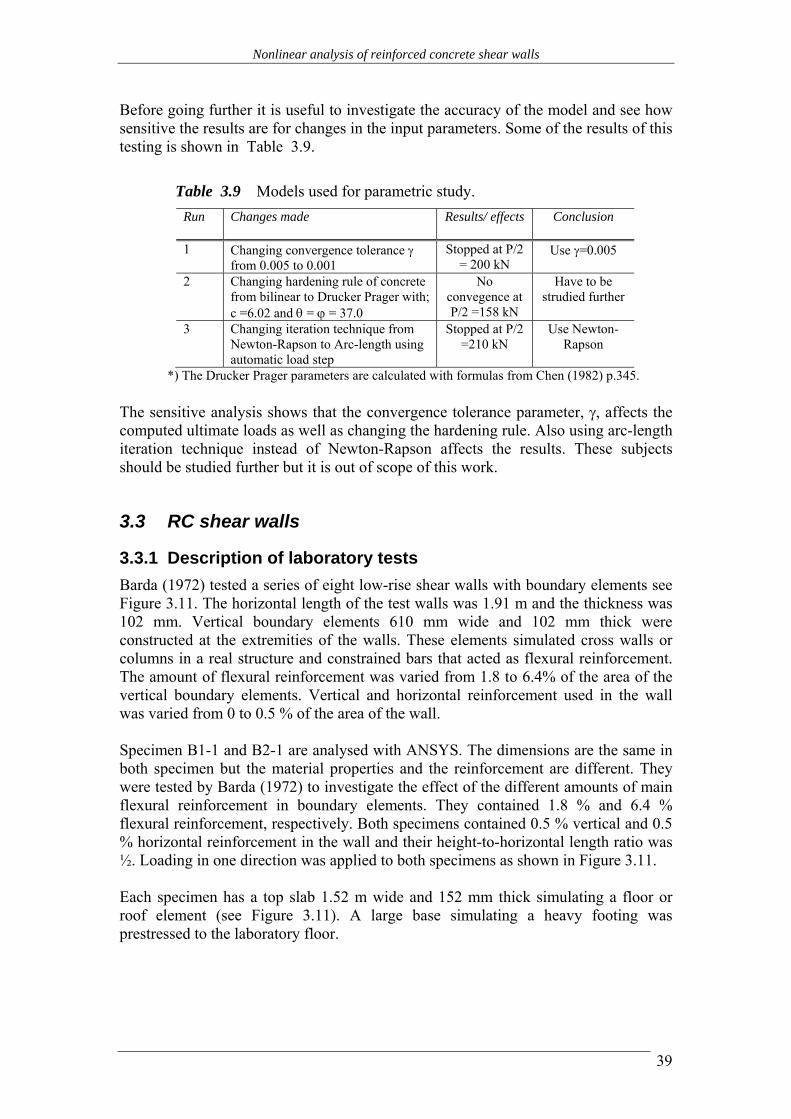
Nonlinear analysis of reinforced concrete shear walls
39
Before going further it is useful to investigate the accuracy of the model and see how sensitive the results are for changes in the input parameters. Some of the results of this testing is shown in Table 3.9.
Table 3.9 Models used for parametric study. Run Changes made Results/ effects
Conclusion
1 Changing convergence tolerance γ from 0.005 to 0.001
Stopped at P/2 = 200 kN
Use γ=0.005
2 Changing hardening rule of concrete from bilinear to Drucker Prager with; c =6.02 and θ = ϕ = 37.0
No convegence at P/2 =158 kN
Have to be strudied further
3 Changing iteration technique from Newton-Rapson to Arc-length using automatic load step
Stopped at P/2 =210 kN
Use Newton-Rapson
*) The Drucker Prager parameters are calculated with formulas from Chen (1982) p.345. The sensitive analysis shows that the convergence tolerance parameter, γ, affects the computed ultimate loads as well as changing the hardening rule. Also using arc-length iteration technique instead of Newton-Rapson affects the results. These subjects should be studied further but it is out of scope of this work.
3.3 RC shear walls
3.3.1 Description of laboratory tests Barda (1972) tested a series of eight low-rise shear walls with boundary elements see Figure 3.11. The horizontal length of the test walls was 1.91 m and the thickness was 102 mm. Vertical boundary elements 610 mm wide and 102 mm thick were constructed at the extremities of the walls. These elements simulated cross walls or columns in a real structure and constrained bars that acted as flexural reinforcement. The amount of flexural reinforcement was varied from 1.8 to 6.4% of the area of the vertical boundary elements. Vertical and horizontal reinforcement used in the wall was varied from 0 to 0.5 % of the area of the wall. Specimen B1-1 and B2-1 are analysed with ANSYS. The dimensions are the same in both specimen but the material properties and the reinforcement are different. They were tested by Barda (1972) to investigate the effect of the different amounts of main flexural reinforcement in boundary elements. They contained 1.8 % and 6.4 % flexural reinforcement, respectively. Both specimens contained 0.5 % vertical and 0.5 % horizontal reinforcement in the wall and their height-to-horizontal length ratio was ½. Loading in one direction was applied to both specimens as shown in Figure 3.11. Each specimen has a top slab 1.52 m wide and 152 mm thick simulating a floor or roof element (see Figure 3.11). A large base simulating a heavy footing was prestressed to the laboratory floor.

Nonlinear analysis of reinforced concrete shear walls
40
Figure 3.11 Tilt up of the test model specimen (Barda, 1972).
The following events were observed in the test of B1-1. Short inclined cracks occurred near the lower left corner of the wall at a load of 22 % of Pu. First shear cracking was considered to have occurred at a load of 42 % of Pu. These cracks were distributed through the middle portion of the wall. At a load of 80 % of Pu, yield of a vertical wall bar was observed. Yield of a horizontal wall bar was observed at a load of 90 % of Pu. The ultimate load Pu is 1205 kN. At the ultimate load, spalling developed along the junction of the top slab and the wall, apparently due to slipping at that junction. This was followed by crushing in the upper left region of the wall, and then in the lower right region of the wall. Nearly all of the wall reinforcement had yielded at ultimate load. After reaching ultimate load the load carrying capacity decreased gradually with increasing lateral displacement. When a lateral deflection of approx. 25.4 mm was reached, the specimen was unloaded (Barda, 1972). The following events were observed in the test of B2-1. A short diagonal crack occurred near the lower left corner of the wall at a load of 22 % of Pu. First shear cracking was considered to have occurred at a load of 31 % of Pu. These cracks were distributed through the middle portion of the wall. At a load of 78 % of Pu, first yield of a horizontal wall bar was observed. Yield of a vertical wall bar was observed at a load of 91 % of Pu. The ultimate load Pu is 997 kN. By the time that the ultimate load was reached, additional diagonal cracks had occurred over the entire wall, and horizontal cracking and spalling started in left part of the wall. Most of the horizontal wall bars yielded at, or just beyond Pu. One third of vertical bars had yielded by the time the Pu was reached. After reaching Pu, the load carrying capacity decreased sharply with increasing lateral deflection (Barda, 1972).
W ll

Nonlinear analysis of reinforced concrete shear walls
41
3.3.2 Analytical results for the shear walls The reinforcement for both wall specimen tested with ANSYS are listed in Table 3.10.
Table 3.10 Reinforcement low rise shear walls B1-1 and B2-1
Reinforcement As/Ac for wall B1-1
As/Ac for wall B2-1
Flanges; vertical reinforcement 1.8 % 6.4 % Flanges: horizontal reinforcement 0.6 % 0.6 % Wall: vertical reinforcement 0.5 % 0.5 % Wall: horizontal reinforcement 0.5 % 0.5 % Slab: parallel to wall 1.2 % 1.2 % Slab: crosswise to wall 1.8 % 1.8 %
The material constants for concrete and steel used are listed in Table 3.11. The stress-strain curves used for concrete and steel material for both wall FE models are similar to those in Figure 3.4 used for the OA1 beam.
Table 3.11 Wall material parameters used in computer models.
Nr Parameter Wall B1-1 Wall B2-1
1 Secant modulus of elasticity (Ec) wall and flanges 23,448 MPa 21,697 MPa 2 Secant modulus of elasticity (Ec) slab 24,092 MPa 17,310 MPa 3 Uniaxial ultimate comp. strength (fc) wall and flanges 29.0 MPa 16.3 MPa 4 Uniaxial ultimate comp. strength (fc) slab 26.3 MPa 21.3 MPa 5 Secant modulus of plasticity (ET) wall and flanges 2310 MPa 1500 MPa 6 Secant modulus of plasticity (ET) slab 2100 MPa 1600 MPa 7 Uniaxial yield strength for concrete 0.8 x fc 0.8 x fc 8 Uniaxial tensile strength (ft) wall and flanges 3.6 MPa 2.2 MPa 9 Uniaxial tensile strength (ft) slab 2.6 MPa 2.3 MPa 10 Ultimate strain for concrete (εu) 3.5 ‰ 3.5 ‰ 11 Shear transfer coefficient for an open crack (βt) 0.1 0.1 12 Shear transfer coefficient for a closed crack (βc) 1.0 1.0 13 Multiplier for amount of tensile stress relaxation (Tc) 0.6 0.6 14 Poisson‘s ratio for concrete (ν) 0.2 0.2 15 Poisson‘s ratio for steel 0.3 0.3 16 Modulus of elasticity for steel (Es) 250,000 MPa 250,000 MPa 17 Modulus of plasticity for steel (Ep) 10,000 MPa 10,000 MPa 18 Yield point of steel (fy) 525 MPa 525 MPa 19 Ultimate strain for steel (εu) 10 ‰ 10 ‰ 20 Weight of steel 77 kN/m3 77 kN/m3 21 Weight of concrete 24 kN/m3 24 kN/m3
Details of the FE model are listed in Table 3.12.

Nonlinear analysis of reinforced concrete shear walls
42
Table 3.12 Finite element model in ANSYS.
Nr Finite element model ANSYS B1-1 and B2-1
1 Dimension of model 3D 2 Total number of concrete elements 472 3 Total number of reinforcement elements 472 4 Cracking and crushing of concrete Yes 6 Load step size Automatic 0.3- 3.0% 7 Gravity load Yes 8 Iteration technique Newton-Rapson 10 Convergence criteria Displacement norm L2,
γ = 0.005 Boundary conditions are shown in Figure 3.12 where the bottom notes are fixed in all directions. Load is distributed on 12 nodes at the slab see Figure 3.12. The top deflection is measured in the top left corner of the wall below the slab.
Figure 3.12 Finite element model used in ANSYS of the low-rise wall with boundary elements.
Figure 3.13 and Figure 3.14 shows the comparison of the FE model and experimental data for the B1-1 and B2-1 shear wall specimen. There it can be observed that the FE model simulates the experiment from B1-1 fairly well but B2-1 very well. The ultimate strength and failure modes of the models agree rather well with experimental results. The initial cracking start to form at similar load level in the experiment and the ANSYS models for both wall specimen. The initial yielding in horizontal and vertical bar was observed in similar spots in the wall as the experiment and the yield load for reinforcement was almost the same as in the experiment. The comparison of the models and experiments are summered up in Table 3.13.

Nonlinear analysis of reinforced concrete shear walls
43
Table 3.13 Comparison of experimental data and FE models.
Initial crack
[% of Pu]
First shear crack
[% of Pu]
Yield of vertical wall bar [% of Pu]
Yield of horizontal wall bar [% of Pu]
Ultimate load [kN]
Experiment B1-1 22 42 80 90 1205 FE model B1-1 30 30 70 - 973 Experiment B2-1 22 31 91 78 997 FE model B2-1 22 - 85 80 1001
0
200
400
600
800
1.000
1.200
1.400
0,0 1,0 2,0 3,0 4,0 5,0 6,0 7,0 8,0Deflection [mm]
Load
[kN
]
Experiment
ANSYS model
Figure 3.13 Comparison of ANSYS models used to model top deflection in wall B1-1.
0
200
400
600
800
1.000
1.200
0,0 1,0 2,0 3,0 4,0 5,0 6,0 7,0
Deflection [mm]
Load
[kN
]
Experiment
ANSYS model
Figure 3.14 Comparison of ANSYS models used to model top deflection in wall B2-1

Nonlinear analysis of reinforced concrete shear walls
44
Further testing showed that if the bilinear model for concrete in compression is replaced with the Drucher-Prager model it is possible to fit the experimental data better at loads above 85 % of ultimate load for B1-1 wall specimen. Also it seems that it is more difficult to fit the experimental data for the B1-1 at lower loads (around 400-600 kN). Similar problem can be found in Ayoub and Filippou (1998). They proposed an orthotropic model for concrete to model RC shear walls and panels, the model includes Ottosen failure criteria (see Figure 2.4), cracking, yielding, softening, aggregate interlock, tension stiffening. They assumed a perfect bond between steel and concrete. They concluded that it is important to include the use of tension stiffening and the use of arc length method if estimating the ultimate strength and failure mode.

Nonlinear analysis of reinforced concrete shear walls
45
4. Nonlinear analysis of shear walls from Icelandic houses
4.1 Introduction
4.1.1 Background In this chapter one story shear walls are analysed nonlinearly. Different reinforcement layouts, amount of reinforcement and concrete strength are used. The selected shear walls are similar to the shear walls in the houses in the South Iceland. The nonlinear finite element model used has been calibrated and verified against experimental data from laboratory tests of both slender reinforced concrete beams and reinforced shear walls as described in chapter 3. At the top of the structure a horizontal load is applied, incrementally, this is called a pushover analysis. These results are presented in a force deformation curve or a capacity curve. There the ductility behavior can be detected, i.e. concrete cracking or crushing and rebar yielding. Furthermore the response is compared to known linear and nonlinear response earthquake spectra taken from the South Icelandic earthquakes of June 2000.
4.1.2 Residential houses in South Iceland Lowland In the years of 1996-1997 a field survey was carried out in the South Iceland Lowland as a part of an earthquake mitigation program called SEISMIS, (Sigbjörnsson et. al., 1998). The objective was to establish data to quantify probable losses in a major earthquake in the South Iceland and to give the house owners an advice regarding earthquake preparedness. The surveying procedure was based upon use of standardized questionnaires and inspection of architectural and engineering drawings. Focusing on the concrete houses the field survey showed that a typical concrete residential house in South Iceland Lowland is symmetric, single story house and is built in the time period 1965-1990. The size of a normal residential house build in this time period is 110 –150 m2. Usually the interior walls are unreinforced brick walls they are 100 mm thick with 10 mm plastering on both sides. The foundations are usually made out of concrete and grounded on rock or gravel. The horizontal rebars are two bars at the wall bottom and the vertical rebars are at c/c 1000 mm, which extend into the exterior wall. The diameter of the rebars is usually 10-12 mm. The concrete material in the wall and the foundation is the same. Sometimes the foundations were made of stonework with some concrete. The floor and roof slab are usually made out of concrete, and have the same concrete strength class as the exterior shear walls. The slab thickness is normally 150 mm. The exterior shear walls are usually 180 mm thick. In houses built before 1980 the concrete strength is usually S200 but in houses built after 1980 it is S250. Plain rebars were used in the concrete prior 1965, but since then deformed (ribbed) rebars have

Nonlinear analysis of reinforced concrete shear walls
46
been used. In the years before 1965 it was common to use only one or two horizontal 12 mm steel bar(s) over openings. In the years from 1965 to 1980 the reinforcement was increased to one or two 12 mm steel bars around the openings. The concrete cover, which is the distance between the outer surface of the reinforcement and the nearest concrete surface, were normally 50-100 mm before 1980. According to EC2 it is 25 mm minimum. After 1980 is was common to use one layer of reinforcement grid in entire wall i.e. 10 mm steel bars c/c 250 mm, and after 1990 double rebars layers were used i.e. 10 mm c/c 250 mm. Figure 4.1 shows an idealized typical symmetrical residential concrete house, which is analysed. Where all the interior walls are non-structural, the exterior walls resist the horizontal earthquake load 2S. It is assumed that the stiffness of the exterior walls is the same and therefore they resist 50 % of 2S respectively, as shown in Figure 4.1. Where it is a capacity analysis each wall can be analysed separately. Here just one exterior wall is analysed.
Figure 4.1 A typical concrete residential house layout, all dimensions are in cm. The house is 120 m2.
S S
2S
Shear walls All interior walls are non bearing
The exterior shear wall analysed

Nonlinear analysis of reinforced concrete shear walls
47
4.2 The analysed RC shear walls from Icelandic houses
4.2.1 The wall types All the walls analysed had the same geometric configuration see Figure 4.2. The wall has two windows and one door. Openings are 27 % of the area and the height versus length (hw/lw) ratio is 0.34. By changing the concrete strength and reinforcement of the wall, twelve different walls were analysed. The different configurations are shown in Table 4.1. Seven walls have the concrete strength S250, W1-W7, and the rest (or five) the concrete strength S200, W1a-W5a. The reinforcement varies from being none to double layers of rebars with additional bars around openings and without boundary reinforcement. The thickness of all the wall types is 180 mm.
8000
1000 1500 1000 1500 1000 1000 1000
500
1250
1000
2750
P 250
Steel beam
Figure 4.2 Dimensions of the analysed shear wall.
Steel beams (angle) are put on the top left corner, where the load is applied, in order to distribute the load at the corner to prevent sudden corner crush. (The dimensions and other parameters for the beams are taken as USP-profil nr. 180 in Teknisk Ståbi (1993)).

Nonlinear analysis of reinforced concrete shear walls
48
Table 4.1 Wall types analysed.
Wall type Concrete type
Reinforcement is equal to; As/Ac vertical
As/Ac horizontal
W1 S250 No reinforcement - - W2 “ 1K12 around openings* - - W3 “ 2K12 around openings - - W4 “ 1K12 c/c250mm in whole wall 0.25 % 0.25 % W5 “ 2K12 c/c250mm in whole wall 0.5 % 0.5 % W6 “ Minimum reinforcement according to
EC2 without reinforcement around openings and boundary. 0.4 % 0.2 %
W7 “ Minimum reinforcement according to EC2 with 2K16 around openings** but no boundary reinforcement. 0.4 % 0.2 %
W1a S200 No reinforcement - - W2a “ 1K12 around openings - - W3a “ 2K12 around openings - - W4a “ 1K12 c/c250mm in whole wall. 0.25 % 0.25 % W5a “ Minimum reinforcement according to
EC2 with 2K16 around openings but no boundary reinforcement. 0.4 % 0.2 %
*) 1K12 = one 12 mm steel bar (As = 113 mm2) **)1K16 = one 16 mm steel bar (As = 201 mm2)
4.2.2 Material properties The reinforcement used in all types is assumed to be marked as S400 steel according to EC2 (see also Figure 2.5), this steel has yield strength of 400 MPa. It is assumed that the S200 concrete is similar to C16 concrete in EC2 with fck = 16 MPa and S250 concrete is similar to C20 concrete with fck = 20 MPa . The fck value is a characteristic cylinder compressive strength defined as 5%-fractile. This is shown schematically in Figure 4.4 where fc is the mean compression strength. % fck fc
Figure 4.3 Standard deviation of typical compressive concrete strength tests.
Compressive concrete strength

Nonlinear analysis of reinforced concrete shear walls
49
It is common to assume that the compressive strength is normal distributed and therefore fck and fc are related by the following equation: fck = fc + 1.64s (4.1) where s is the standard deviation. The standard deviation is estimated as 3-5 N/mm2 (CEN, 1991). According to Eq. (4.1) the mean compressive strength for S200 concrete with fck as 16 MPa and S250 concrete with fck as 20 MPa are as follows:
S200: fc = fck + 1.64s = fck + (5-8 MPa) = 21 – 24 MPa S250: fc = fck + 1.64s = fck + (5-8 MPa) = 25 – 28 MPa
It is decided to use the lower limit, fc = 21 MPa, for uniaxial ultimate compressive strength for S200 concrete strength and fc = 25 MPa for S250 concrete strength. The secant modulus of elasticity, Ec, and uniaxial tension strength, ft, is calculated according to Eq. (2.1) and (2.2), respectively. The material properties for the wall types are listed in Table 4.2 for both concrete strength, i.e. S200 and S250.
Table 4.2 Material parameters used in the analysis.
Nr Parameter S200 concrete
S250 concrete
1 Secant modulus of elasticity (Ec) 27,403 MPa 28,847 MPa 2 Uniaxial ultimate comp. strength (fc) 21.0 MPa 25.0 MPa 3 Uniaxial tensile strength (ft) 1.9 MPa 2.2 MPa 4 Secant modulus of plasticity (ET) 1,481 MPa 1,852 MPa 5 Uniaxial yield strength for concrete 0.8 x fc 0.8 x fc 6 Ultimate strain for concrete (εu) 3.5 ‰ 3.5 ‰ 7 Shear transfer coefficient for an open crack (βt) 0.1 0.1 8 Shear transfer coefficient for a closed crack (βc) 1.0 1.0 9 Multiplier for amount of tensile stress relaxation (Tc) 0.6 0.6 10 Poisson‘s ratio for concrete (ν), elastic and cracked 0.2 0.2 11 Poisson‘s ratio for steel 0.3 0.3 12 Modulus of elasticity for steel (Es) 200.000 MPa 200.000 MPa 13 Modulus of plasticity for steel (Ep) 1.035 MPa 1.035 MPa 14 Yield point of steel (fy) 400 MPa 400 MPa 15 Ultimate strain for steel (εu) 15 ‰ 15 ‰ 16 Weight of steel 77 kN/m3 77 kN/m3 17 Weight of concrete 24 kN/m3 24 kN/m3

Nonlinear analysis of reinforced concrete shear walls
50
4.2.3 Analytical nonlinear model The analytical model of the wall is shown in Figure 4.4. All nodes at the ground level are fixed. Table 4.3 shows the main characteristics of the FE-model used in ANSYS.
Figure (a)
Figure (b)
Figure 4.4 Element model in ANSYS of the wall types a) the analytical model three dimensional view and b) element numbers.

Nonlinear analysis of reinforced concrete shear walls
51
Table 4.3 Finite element model of wall types.
Nr Finite element model ANSYS wall model
1 Dimension of model 3D 2 Total number of concrete elements 256 3 Total number of beam elements 8 4 Total number of reinforcement elements 0-256 5 Cracking and crushing of concrete Yes 6 Yielding of concrete and reinforcement Yes 7 Bond slip between steel and concrete No 8 Load step size 10 kN 9 Gravity load Yes 10 Iteration technique Newton-Rapson 11 Convergence criteria Displacement norm,
γ = 0.005
4.2.4 Applied loading The horizontally load, P, is monotonic and applied slowly (stepwise) at the top of the wall. The load is applied on the top two nodes. In addition the self-weight of the structure is included in the analysis i.e. gravity load of the wall and constant vertical load from the roof. The vertical load from the roof is from the concrete slab, which is assumed to be 150 mm thick with an isolation and roofing. The total square meters of the roof are 120 m2. It is assumed that the load from 10 % of the roof is acting vertically on the sidewall. The total vertical load is 44 kN and the load is distributed on all nodes on the top of the wall. In subsequent analysis the load P is normalized with the tributary weight, S, which act as an earthquake loading on the wall (see Figure 4.1) and is estimated as follows; (a) The total dead load from the roof, Sroof, is 510 kN and half of it is resisted by the shear wall. (b) The total dead load from the wall, Swall, is 72 kN and half of it is resisted by the shear wall. (c) No live load is assumed to act on the roof during earthquake. The total load is therefore, ⇒ S = (Sroof+ Swall)/2 = 255 kN + 36 kN = 291 kN
4.2.5 Analytical results for S250 concrete walls Figure 4.5 shows the load – defection curve or, the capacity curve for the wall types W2 to W7. The top deflection is defined as horizontal displacement of the top left corner. Reinforcement is defined in Table 4.1. In Figure 4.6 the horizontal force is normalized with the tributary weight, S = 291 kN, see chapter 4.2.4. The displacement is normalized in the forms of displacement ductility as prescribed in chapter 2.3. The displacement ductility μ is one when the wall starts to yield. The yield deflection Δy is the same for all wall types i.e. 0.44 mm.

Nonlinear analysis of reinforced concrete shear walls
52
As seen in Figure 4.5 and Figure 4.6 all curves have been cut off at deflection of 6 mm and at ductility of 12 although all wall type result a higher ultimate deflection and load. This is done because at ductility 8 the structure stability is treated by buckling, brittle failure etc. as seen in Figure 2.7. The ultimate top displacement is approximately 7-8 mm and 10-12 mm for walls W2-W3 and W4-W7, respectively. The corresponding ultimate load is approximately 400-500 kN and 800-1000 kN for walls W2-W3 and W4-W7, respectively. Increasing the reinforcement increases the wall resistance. For instance by focusing on the ductility at 8 for wall W2 the normalized applied load is 1.3 and the corresponding increase (in percent) in the applied load for walls W3, W4, W5, W6, W7 at same ductility is 15%, 30%, 57%, 40% and 70%, respectively. If we compare the ductility of the walls when the applied normalized load is 1.3 the ductility for the walls W3-W7 is 5, 3.8, 2.8, 3 and 2.5, respectively. All wall types started the initial cracking at the load of 240 kN or normalized load (P/S) of 0.825. Type W1 is not plotted on the figures where it became unstable right after yielding. Walls with little reinforcement i.e. walls W2-W4 and W5 develop a shear failure near initial cracking load.
0
100
200
300
400
500
600
700
800
900
0,0 1,0 2,0 3,0 4,0 5,0 6,0Deflection [mm]
Load
[kN
]
W7; EC2 + 2K16 openingsW5; 2xK12 c/c250W6; reinforcement EC2W4; 1xK12 c/c250W3; 2xK12 around openingsW2; 1xK12 around openingsLinear-elastic
Figure 4.5 Load – deflection curves for varying reinforcement and S250 concrete.

Nonlinear analysis of reinforced concrete shear walls
53
0,0
0,5
1,0
1,5
2,0
2,5
3,0
0 1 2 3 4 5 6 7 8 9 10 11 12
Nor
mal
ized
load
( P
/S)
W7; EC2 + 2K16 openingsW5; 2xK12 c/c250W6; reinforcement EC2W4; 1xK12 c/c250W3; 2xK12 around openingsW2; 1xK12 around openingsLinear-elastic
Figure 4.6 Normalized load – ductility curves for varying reinforcement and S250 concrete.
Figure 4.7(a) shows how the shear wall W7 deforms from the structural selfweight i.e. the roof and the wall weight. The maximum vertical deflection is over the window and is 0.02 mm. The deformation figures are similar for all the other walls. In Figure 4.7 (b), is shown the horizontal deflection for wall W7 at ductility 3.
Figure (a) – self-weight loading
Figure (b) – lateral loading
Figure 4.7 Vertical and horizontal deformation for wall W7 a) vertical deformation from self weight loads b) horizontal displacement from lateral load at ductility 3.
Displacement ductility

Nonlinear analysis of reinforced concrete shear walls
54
It is also possible to see how the steel stress changes in the walls. Table 4.4 shows where and for what loading the first vertical rebar bar starts to yield in all the walls. Some results are also presented with respect to wall W2 results. Wall W7 can carry 250 % more horizontal load than wall W2, before the steel starts to yield and the corresponding ductility increases by 278%. The W6 wall shows lower ductility and load increase when yield start compared to W5 wall. This is due to the amount of horizontal reinforcement, in wall W6 it is ρ=0.002 but ρ=0.005 in wall W5. Wall W4 shows reduction in ductility when rebars start to yield compared to wall W2 but an increase in load capacity of 30%. Table 4.4 shows also a damage column. This is the damage when steel yields at a certain normalized load. The damage in a wall is defined as the cracked area divided by the wall area. The cracked area is found by counting the total number of cracked concrete elements in the model. The total number of concrete elements is used for the wall area i.e. 256 (see Table 4.3). By doing this for number of load steps the curves on Figure 4.11 and Figure 4.12 can be drawn. Figure 4.11 shows damage – normalized load curves for walls W2-W7 and Figure 4.12 shows damage – ductility curves for walls W2-W7. It is better to see the difference between the wall types damage in Figure 4.11, for instance at normalized load level of 1.0 the wall W2 has a damage of 18% while wall W7 has only 5 % damage.
Table 4.4 Wall ductility and damage when the vertical reinforcement yields.
Wall type
Element to yield see
Fig. 4.4(b)
P/S when steel
yields
Ductility μ when steel
yields
P/S increase ref. to W2
[%]
μ increase ref. to W2
[%]
Damage see Fig. 4.11 and
4.12 [%] W1 - - - - - - W2 101 1.0 3.8 - - 18 W3 157 1.5 6.0 50 58 32 W4 161 1.3 3.6 30 - 5 16 W5 101 2.3 10.2 230 261 56 W6 161 1.6 4.6 160 21 18 W7 161 2.5 10.6 250 278 60
Table 4.5 shows that when walls W2, W5 and W7 reach their ultimate load none of the horizontal reinforcement has yielded. When yielding is observed in wall W3, W4 and W6 the damage is 57% or more.
Table 4.5 Wall ductility and damage when the horizontal reinforcement yields.
Wall type
Element to yield see
Fig. 4.4(b)
P/S when steel yields
Ductility μ when steel
yields
Damage see Fig. 4.11 and
4.12 [%]
W1 - - - - W2 171 - - - W3 180 1.7 16 57 W4 28/181 2.2 16 60 W5 28/181 - - - W6 181 2.6 7.2 65 W7 181 - - -

Nonlinear analysis of reinforced concrete shear walls
55
Figure 4.8 shows steel stresses versus normalized load for vertical reinforcement in element 101 see Figure 4.4(b). It can clearly be seen how fast the steel stresses in W2 increases compared to all the other walls.
0
50
100
150
200
250
300
350
400
450
0,0 0,5 1,0 1,5 2,0 2,5 3,0 3,5
Normalized load (P/S)
Stee
l str
ess
[MPa
]
1xk12 around openings1xK12 c/c2502xk12 around openingsReinforcement EC22xK12 c/c250EC2 +2K16 around open.Linear-elastic
Figure 4.8 Steel stresses – normalized load curves in vertical rebars in element 101 (see Figure 4.4 (b)).
By viewing the values in Table 4.4 and Table 4.5 it can be observed that the lower limit of the damage when yielding occurs is around 16-18 %. In Table 4.6 the normalized load (P/S) and the ductility is computed for 18% damage level. There the ductility is almost the same for wall W2-W5 but in walls W6 and W7 it is about 20% higher. The same is observed for the load capacity the load increase is 15% to 70% for walls W3-W7.
Table 4.6 Wall properties for fixed damage of 18%.
Wall type Normalized load (P/S)
value
Ductility μ P/S increase ref. to W2
[%]
μ increase ref. to W2
[%] W1 - - - - W2 1.0 3.8 - - W3 1.15 3.6 15 -5 W4 1.25 3.9 25 3 W5 1.55 3.9 55 3 W6 1.6 4.6 60 21 W7 1.7 4.5 70 19
Figure 4.9 shows cracks and corresponding principle stresses for wall W2 for four normalized load levels, i.e. 0.82, 0.86, 1.0 and 1.4. This wall has just one bar around openings. From the principle stress figures it can been seen how the compression

Nonlinear analysis of reinforced concrete shear walls
56
force acting on the top of the wall spreads inside the wall from corner to corner and between windows. The main tension struts and compression struts are also observed. The crack sequence can be determined in Figure 4.9(b), (d) and (e). They start at the window corners and where the main tension struts are. The secondary cracks also start, which implies a brittle failure in the concrete. When the reinforcement yields in Figure 4.9(d) at P/S as 1.0, the secondary cracks have developed in element 101 (left window, lower right corner) implying that there is a danger of bond slip effects, since the secondary cracks are nearly parallel with the rebars. Further there are two elements (nr. 161 and 101) that are cracked in three directions, which imply an unstable condition. The crack pattern in Figure 4.9(e) shows quite many cracked elements in three directions (total of eleven) implying a unstable conditions, for instance the strain in element 181 is 0.0114 indicating a crack width of 3 mm.
Figure (a) – P/S=0.82
Figure (b) - P/S=0.86
Figure (c) – P/S=0.86

Nonlinear analysis of reinforced concrete shear walls
57
Figure (d) – P/S=1.0
Figure (e) – P/S=1.4
Figure (f) – P/S=1.4
Figure 4.9 Wall W2 analytical model a) principal stress orientation before cracking P/S = 0.82 b) initial cracks in concrete P/S = 0.86 c) principal stress at P/S=0.86 d) cracks in concrete at P/S = 1.0 e) cracks in concrete at P/S = 1.4 f) principal stress at P/S = 1.4.
Figure 4.10 shows crack pattern for the W7 wall i.e. P/S = 0.86 and P/S = 2.5. When P/S = 0.86 cracks are minor and at P/S = 2.5 the vertical rebars starts to yield and only two elements has cracked in all directions, but many elements cracked into two directions.
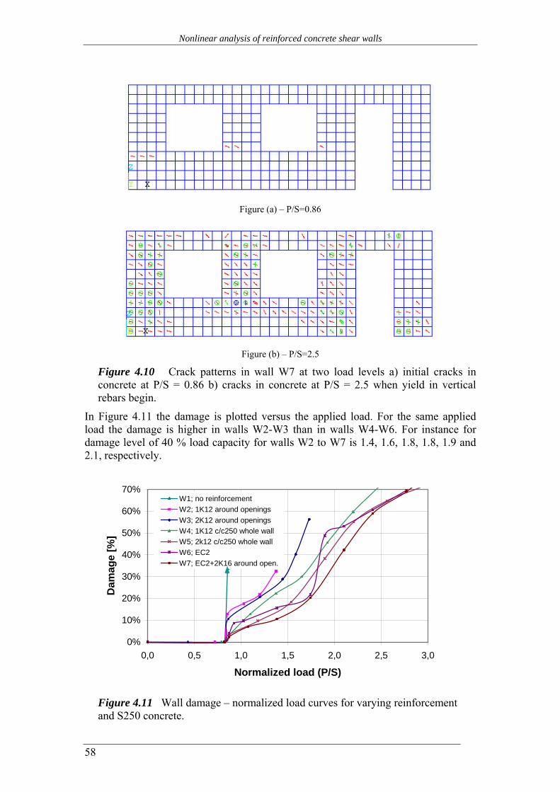
Nonlinear analysis of reinforced concrete shear walls
58
Figure (a) – P/S=0.86
Figure (b) – P/S=2.5
Figure 4.10 Crack patterns in wall W7 at two load levels a) initial cracks in concrete at P/S = 0.86 b) cracks in concrete at P/S = 2.5 when yield in vertical rebars begin.
In Figure 4.11 the damage is plotted versus the applied load. For the same applied load the damage is higher in walls W2-W3 than in walls W4-W6. For instance for damage level of 40 % load capacity for walls W2 to W7 is 1.4, 1.6, 1.8, 1.8, 1.9 and 2.1, respectively.
0%
10%
20%
30%
40%
50%
60%
70%
0,0 0,5 1,0 1,5 2,0 2,5 3,0
Normalized load (P/S)
Dam
age
[%]
W1; no reinforcementW2; 1K12 around openingsW3; 2K12 around openingsW4; 1K12 c/c250 whole wallW5; 2k12 c/c250 whole wallW6; EC2W7; EC2+2K16 around open.
Figure 4.11 Wall damage – normalized load curves for varying reinforcement and S250 concrete.

Nonlinear analysis of reinforced concrete shear walls
59
From Figure 4.12 it can be seen that in the beginning of damage the curves for W2-W4 and W6 shows higher damage than the curves for W5 and W7.
0%
10%
20%
30%
40%
50%
0 1 2 3 4 5 6 7 8
Dam
age
[%]
W2; 1K12 around openingsW3; 2K12 around openingsW4; 1K12 c/c250 whole wallW5; 2k12 c/c250 whole wallW6; EC2W7; EC2+2K16 around open.
Figure 4.12 Wall damage – displacement ductility for varying reinforcement and S250 concrete.
4.2.6 Analytical results for S200 concrete walls Figure 4.13 shows the load – deflection curve or the capacity curve for the walls W2a to W5a. As before the capacity curve shows the horizontal displacement of the upper left corner as a function of the horizontal force P (see Figure 4.2). The initiation of crack is the same for all walls i.e. 0.40 mm. As seen in Figure 4.13 and Figure 4.14 all curves have been cut down at the deflection of 6 mm or ductility level 12 as in chapter 4.2.5. The ultimate deflection is approximately 6 mm and 8-10 mm for walls W2a-W3a and W4a-W5a, respectively. The corresponding ultimate load is approximately 380-450 kN and 900-700 kN for walls W2a-W3a and W4a-W5a, respectively. Increasing the reinforcement increases the wall resistant. For instance by focusing on the ductility at 8 for wall W2a the normalized applied load P/S is 1.2 and the corresponding increase (in percent) in the applied load for walls W3a, W4a and W5a at same ductility is 17%, 30% and 60%, respectively. If we compare the ductility of the walls when the applied load is (P/S) 1.2 the ductility for the walls W3a-W5a and linear-elastic model is 4.5, 4.0, 2.7 and 1.6. All wall types started to crack at the load of 210 kN or normalized load P/S of 0.72, which is 13 % lower limit then accomplish by S250 concrete in chapter 4.2.5. Wall W1a is not plotted on the figures where it became unstable right after yielding. Walls with little reinforcement i.e. walls W2a-W4a develop a shear failure near initial cracking load.
Displacement ductility

Nonlinear analysis of reinforced concrete shear walls
60
0
100
200
300
400
500
600
700
800
0,0 1,0 2,0 3,0 4,0 5,0 6,0
Deflection [mm]
Load
[kN
]
W5a; EC2+2K16 around opW4a; 1K12 c/c250W3a; 2K12 around open.W2a; 1K12 around open.Linear-elastic
Figure 4.13 Load – deflection curves for varying reinforcement and S200 concrete.
0,0
0,2
0,4
0,6
0,8
1,0
1,2
1,4
1,6
1,8
2,0
0 1 2 3 4 5 6 7 8
Nor
mal
ized
load
(P/S
)
W5a; EC2+2K16 around op W4a; 1K12 c/c250W3a; 2K12 only openingsW2a; 1K12 only openingsLinear elastic
Figure 4.14 Normalized load – ductility curves for varying reinforcement and S200 concrete.
It is also possible to see how the steel stress changes in the walls. Table 4.7 shows where and for what loading the first vertical rebar starts to yield in all the walls. Some results are also presented with respect to wall W2a results. Wall W5a can carry 240 % more horizontal load than wall W2a, before the steel starts to yield and the
Displacement ductility

Nonlinear analysis of reinforced concrete shear walls
61
corresponding ductility increases by 250%. The W4a wall shows lower ductility when steel yield start compared with W2a wall but increase in load capacity of 20%. In Table 4.7 there is also a damage column that refers to Figure 4.16 and Figure 4.17. For instance when yielding in W2a is observed damage is 20%. Figure 4.16 shows wall damage – normalized load curves for walls W2a-W5a and Figure 4.17 shows wall damage – displacement ductility curves for walls W2a-W5a. It is better to see the difference between the wall types damage in Figure 4.16, for instance at normalized load level of 1.0 the W2a has a damage of 20% while W5a has only 7 %, W4a 11% and W3a 16%.
Table 4.7 Wall ductility and damage when the vertical reinforcement yields.
Wall type
Element to yield see
Fig. 4.4(b)
P/S when steel yields
Ductility μ when steel
yields
P/S increase ref. to W2
[%]
μ increase ref. to W2
[%]
Damage see Fig. 4.16 and
4.17 [%] W1a - - - - - - W2a 101/108 1.0 4.9 - - 20 W3a 101 1.4 6.4 40 31 32 W4a 161 1.2 3.8 20 - 29 17 W5a 161 2.4 12.1 240 250 60
Table 4.8 shows comparison when first horizontal reinforcement yields, as seen in the table there was no yield observed in walls W2a, W3a and W5a at ultimate load. When yielding was observed in wall W4a the cracking damage is 60%.
Table 4.8 Wall ductility and damage when the horizontal reinforcement yields.
Wall type
Element to yield see
Fig. 4.4(b)
P/S when steel yields
Ductility μ when steel
yields
Damage see Fig. 4.16 and
4.17 [%] W1a - - - - W2a 171 no yield - - W3a 180 no yield - - W4a 181 3.9 20 60 W5a 181 no yield - -
Figure 4.13 shows steel stresses versus normalized load for vertical reinforcement bar (s) in element 101 see Figure 4.4(b). It can clearly be seen how fast the steel loading is in W2a increase compared to all other walls.

Nonlinear analysis of reinforced concrete shear walls
62
0
50
100
150
200
250
300
350
400
450
0,0 0,5 1,0 1,5 2,0 2,5 3,0
Normalized load (P/S)
Stee
l str
ess
[MPa
]
W2a; 1K12 around openingsW3a; 2K12 around openingsW4a; 1K12 c/c250W5a; EC2+2K16 around opLinear-elastic
Figure 4.15 Steel stresses– normalized load curves for vertical reinforcement in element 101 see Figure 4.4(b).
By viewing the values in Table 4.7 and Table 4.8 it can be observed that the lower limit of the damage when yielding occurs is around 20%. In Table 4.9 the normalized load and the ductility is compared for 20% damage level. There the ductility increase about 10-20% for walls W3a-W5a, with ref. to wall W2a. The same is observed for the load capacity the load increase is 20 to 50% for walls W3a-W5a.
Table 4.9 Wall properties for fixed damage of 20 %.
Wall type
Normalized load (P/S)
value
Ductility μ
P/S increase ref. to W2a
[%]
μ increase ref. to W2a
[%] W1a 0.7 - - - W2a 1.0 4.2 - - W3a 1.2 4.6 20 10 W4a 1.3 4.8 30 15 W5a 1.5 5.0 50 20
In Figure 4.16 the damage is plotted versus the applied load. For the same applied load the damage is higher in walls W2a-W4a than in wall W5a. For instance at a damage level of 40 % the load capacity P/S for W2a-W5a is 1.25, 1.35, 1.65 and 1.95, respectively.

Nonlinear analysis of reinforced concrete shear walls
63
0%
10%
20%
30%
40%
50%
60%
70%
0,0 0,5 1,0 1,5 2,0 2,5 3,0
Normalized load (P/S)
Dam
age
[%]
W2a; 1K12 around open. W3a; 2K12 around open.W4a; 1K12 c/c250W5a; EC2+2K16 around opW1a; no reinforcement
Figure 4.16 Wall damage – normalized load curves for varying reinforcement and S200 concrete.
From Figure 4.17 it can be seen that in the beginning of damage the curves for W2a-W4a shows higher damage than the curves for W5a.
0%
10%
20%
30%
40%
50%
60%
0,0 2,0 4,0 6,0 8,0 10,0 12,0
Dam
age
[%]
W2a; 1K12 around open.
W3a; 2K12 around open.
W4a; 1K12 c/c250
W5a; EC2+2K12 around op
Figure 4.17 Wall damage – ductility curves for varying reinforcement and S200 concrete.
Displacement ductility

Nonlinear analysis of reinforced concrete shear walls
64
4.3 The South Iceland Earthquakes June 2000 – demand vs. capacity
4.3.1 Introduction In this chapter the capacity of all the analysed walls, W1-W7 and W1a-W5a, are compared to the measured earthquake loading of two major earthquakes in the South Iceland Lowland in June 2000. The first earthquake was on June with magnitude 6.5. The earthquake-induced damage in the epicentral area was considerable, especially in the village Hella. There were structural damages on buildings and their interior articles as well as piping systems (Sigbjörnsson, et. al., 2000). The recorded peak ground acceleration at Hella was 47% g. The highest recorded peak ground acceleration was 64% g on the farm Kaldárholt. The recorded peak ground accelerations were measured by the Earthquake Engineering Research Center of the University of Iceland that operates the Strong Motion Network in South Iceland (Thórarinsson, et.al., 2000). The second earthquake magnitude was on June 21 with magnitude 6.5. The highest recorded peak ground acceleration was 84% g on the western site of the Thjórsár-Bridge approximately 5 km from the epicenter. The earthquake-induced damage in the epicentral area is considerable, especially on farm houses and summer cottages.
4.3.2 Elastic and nonlinear response spectra In Figure 4.18 and Figure 4.19 the elastic and nonlinear earthquake response spectra are shown at Hella and Kaldaárholt (Sigbjörnsson et. al., 2000).
Se
ism
ic c
oeff
icie
nt [%
g]
0 0.2 0.4 0.6 0.8 10
50
100
150
200
250
JAR
ÐS
KJÁ
LFT
AS
TU
ÐU
LL (
% g
)
2%
5%
20%
Undamped natural period [s] Figure (a)
S
eism
ic c
oeff
icie
nt [%
g]
0 0.2 0.4 0.6 0.8 10
100
200
300
400
500
600
JAR
ÐS
KJÁ
LFT
AS
TU
ÐU
LL (
% g
)
2%
5%
20%
Undamped natural period [s] Figure (b)
Figure 4.18 Elastic earthquake response spectra: Earthquake 17 June 2000, 15:41. Seismic coefficient –undamped natural period curve for critical damping ratio: 2%, 5% and 20% at (a) Hella, (b) Kaldárholt (Sigbjörnsson et. al., 2000).

Nonlinear analysis of reinforced concrete shear walls
65
Sei
smic
coe
ffic
ient
[% g
]
0 0.2 0.4 0.6 0.8 110
20
30
40
50
60
70
80
90
ÓDEYFÐUR EIGINSVEIFLUTÍMI (s)
JAR
ÐS
KJÁ
LFT
AS
TU
ÐU
LL (
% g
)
μ = 2
μ = 3
μ = 4
Undamped natural period [s] Figure (a)
S
eism
ic c
oeff
icie
nt [%
g]
0 0.2 0.4 0.6 0.8 10
20
40
60
80
100
120
140
ÓDEYFÐUR EIGINSVEIFLUTÍMI (s)
JAR
ÐS
KJÁ
LFT
AS
TU
ÐU
LL (
% g
)
μ = 2
μ = 3
μ = 4
Undamped natural period [s] Figure (b)
Figure 4.19 Nonlinear earthquake response spectra: Earthquake 17 June 2000, 15:41. Seismic coefficient – undamped natural period curve for critical damping ratio:2% and ductility coefficient μ : 2, 3 and 4 at (a) Hella, (b) Kaldárholt (Sigbjörnsson et. al., 2000).
4.3.3 Demand versus capacity for the analysed shear walls In Table 4.10 the seismic coefficient is estimated from Figure 4.18 and Figure 4.19 for ductility coefficient 1 (elastic), 2, 3 and 4, supposing the undamped natural period of the walls to be 0.05-0.2 s. It should be kept in mind that when a wall cracks the undamped natural period becomes larger. The viscous damping is assumed to be 5 % for the elastic system and 2% for the nonlinear system (Eurocode 8, 1995, and Paulay & Priestley, 1992).
Table 4.10 Comparison of seismic coefficient for Hella and Kaldárholt, supposing the undamped natural period to be 0.05-0.2 s.
Suppose that the wall stand
on:
Damping [%]
Ductility coefficient
μ
Seismic coefficient,
[g] Hella 5 1 1.0
“ 2 2 0.8 “ 2 3 0.6 “ 2 4 0.5
Kaldárholt 5 1 3.0 “ 2 2 1.2 “ 2 3 1.0 “ 2 4 0.8
In Figure 4.20 and Figure 4.21 the table values from Table 4.10 are drawn both for Kaldárholt and Hella. By drawing these values onto the same chart as the capacity curves are for wall types both for S250 and S200 respectively (see Figure 4.6 and Figure 4.14) we get a demand curve as seen in Figure 4.20 and Figure 4.21.

Nonlinear analysis of reinforced concrete shear walls
66
0,0
0,2
0,4
0,6
0,8
1,0
1,2
1,4
1,6
1,8
2,0
2,2
0 1 2 3 4 5 6 7 8
Nor
mal
ized
load
(P/S
)
W7; EC2+2K16 openingsW6; 2xK12 c/c250W5; EC2W4; 1xK12 c/c250W3; 2xK12 around openingsW2; 1xK12 around openingsLinear-elastic Demand curve - KaldárholtDemand curve - Hella
Figure 4.20 Capacity curves versus the demand curves for S250 concrete.
0,0
0,2
0,4
0,6
0,8
1,0
1,2
1,4
1,6
1,8
2,0
0 1 2 3 4 5 6 7 8
Nor
mal
ized
load
(P/S
)
W5a; EC2+2K16 open. W4a; 1xK12 c/c250W3a; 2xK12 only openingsW2a; 1xK12 only openingsLinear elasticDemand curve - KaldárholtDemand curve - Hella
Figure 4.21 Capacity curves versus the demand curves for S200 concrete.
It can be seen from Figure 4.20 and Figure 4.21 that were the demand curves intersect the capacity curves for the wall type we get the critical values both for both ductility and load for each wall type. From that we can get the damage by reviewing Figure 4.11 for S250 concrete and Figure 4.16 for S200 concrete. These values are summered
Displacement ductility
Displacement ductility

Nonlinear analysis of reinforced concrete shear walls
67
up in Table 4.11 and Table 4.12 for Kaldárholt, where LE model refers to the Linear-Elastic model without any damage. By comparing the tables it can be observed that the damage is more in the wall with S200 concrete than in S250 wall types. Furthermore the W2 and W2a walls result in twice as much damage (or repairing cost) compared with W7 and W5a after an major earthquake. At this demand curve all wall type has received cracking in concrete, but no crushing or reinforcement yield has taken place. Type W1 and W1a would have been heavily damaged and W2a-W4a and W2-W5 probably have developed shear cracking. Finally, having in mind that the walls have received permanent displacement and cracking they are weaker to challenge another major earthquake. It may therefore be necessary to not only repair the walls but also strengthening them. The strengthening and repair analysis of the walls can be carried out with the use of the FE model but that part is beyond the scope of this work. Guidelines for strengthening and repair analysis for shear walls can be found in Penelis and Kappos (1997), Zsutty (1995) and Lombard (2000).
Table 4.11 Comparison when demand curve intersect the capacity curve for S250 concrete for Kaldárholt.
Wall type
Seismic coefficient
[g]
Ductility μ Seismic coefficient
increase ref. to W2a [%]
Ductility decrease
ref. to W2a [%]
Damage see Fig. 4.11 and
4.12 [%]
W1 - - - - - W2 0.92 3.3 - - 16 W3 1.02 2.9 11 -12 15 W4 1.06 2.7 15 -18 12 W5 1.10 2.5 20 -24 8 W6 1.14 2.3 24 -30 11 W7 1.15 2.2 25 -33 8 LE 1.55 1.8 69 -45 0
Table 4.12 Comparison when demand curve intersect the capacity curve for S200 concrete for Kaldárholt.
Wall type
Seismic coefficient
[g]
Ductility μ Seismic coefficient
increase ref. to W2a [%]
Ductility decrease
ref. to W2a [%]
Damage see Fig. 4.11 and
4.12 [%]
W1a - - - - - W2a 0.86 3.7 - - 18 W3a 0.94 3.3 9 -11 14 W4a 1.00 3.0 16 -19 12 W5a 1.10 2.5 28 -32 9 LE 1.40 1.9 63 -51 0

Nonlinear analysis of reinforced concrete shear walls
68
Nonlinear analysis of reinforced concrete shear walls
69
5. Summary and conclusions The program ANSYS turned out to be a good analytical tool for analysing nonlinear concrete walls. Two other programs were also used, but modelling and analysing concrete prototypes, the program ANSYS showed the best correlation with the experimental results. The main reason why ANSYS showed the best performance is its ability to model tensile cracks in concrete. This was noted after a numerical simulation of a beam without shear reinforcement. The program was then used to simulate response test results of beam with shear reinforcement and of two different low rise shear wall types. The FE model tracks the response of the reinforced beams with or without shear reinforcement very accurately. Modelling of the first shear wall was fairly good and modelling of the second shear wall was very good. This analytical tool gives useful information about the behavior of reinforced concrete elements under monotonic loading. The analysis detects concrete initial cracks, shear cracks and crushing, and rebar deformations as well as damage ratio. Determination of ultimate load is more difficult as it is affected by hardening rule, convergence criteria and iteration method used. It should be noted that each experiment considered was only based on one test, therefore no bonds or standard deviation of the results are available. It is likely that repeated tests would have some variations. A nonlinear finite element model was constructed to analyse capacity of several reinforced concrete shear walls with openings in a typical one story residential house. The analysis is carried out statically where the load is stepwise increased. This phenomenon is usually called pushover analysis and results in complete force deformation curves or capacity curves. Twelve wall types were tested, seven had S250 concrete and five S200 concrete. All had different reinforcement. The reinforcement varied from being nothing to EC2 minimal requirements without boundary reinforcement. Results clearly indicate that changing the reinforcement greatly affect the response. The analysis indicated that walls with the same concrete strength form cracks at the same load level and the vertical reinforcement yielded prior the horizontal reinforcement. Walls with little reinforcement developed shear failure right after the initial crack load. The analysis also indicated that the ductility and shear strength of the shear wall is highly affected by the reinforcement around openings and the boundary reinforcement is crucial to avoid shear cracking. It was noticed that well reinforced shear walls distributed the cracks over a greater area than the poor reinforced walls. The capacity curves for the shear walls were compared to the demand curves as developed from the South Icelandic earthquakes of June 2000. The spectra were based on recorded data from Kaldárholt and Hella. This comparison indicated that the unreinforced walls would have been heavily damaged at those sites. Walls with little reinforcement would probably have developed shear cracking, while well reinforced walls would suffer minimal damage. To improve the analytical model and to obtain a better estimation of ultimate load, it is recommended as next steps to consider the rebar bond slip phenomenon and to study the effect of element size, iteration method and convergence criteria. In further study shear walls with different geometric configurations, rebars layout and material properties should be analysed. The use of dynamic loading instead of

Nonlinear analysis of reinforced concrete shear walls
70
monotonic should also be tested. Finally, an analysis of existing shear walls, which failed in the South Iceland Lowland Earthquake of June 2000, should be studied. Nonlinear analysis is realistic and reliable method for evaluating the structural response of reinforced concrete structures in seismic zones. It is though rather complex and time consuming. The method can be used in design of new structures and in repairing and retrofitting of structures as well as in code calibration, and in risk assessment.

Nonlinear analysis of reinforced concrete shear walls
71
6. References ANSYS Engineering Analysis System (1998): User and Theoretical Manual. ANSYS, Inc.
Southpointe, Canonsburg, Pennsylvania, USA, Version 5.6.2. ASCE Committee 447 on Finite Element Analysis of Reinforced Concrete (1994): State-of-
the-art report on finite element analysis of reinforced concrete, ASCE. Ayoub, A. and Filippou, F.C.(1998): Nonlinear Finite Element Analysis of RC shear panels
and walls. Journal of structural engineering, Vol.124, No.3, March, 1998. ASCE. Barda, F. (1972): Shear strength of low-rise walls with boundary elements. Ph.D. Thesis,
Lehigh University, Bethlehem, Pennsylvania, USA. Bresler, B. and Scordelis, A.C. (1964), Shear strength of reinforced concrete beams. Insittiue
of Engineering research University of California Berkeley, California. CEN Techn. Comm. 250 SG2 (1991) Eurocode 2: Design of Concrete Structures-Part 1:
General Rules and Rules for Buildings (ENV 1992-1-1), CEN, Berlin. CEN Techn. Comm. 250 SC8 (1995) Eurocode 8: Earthquake Resistant Design of Structures-
Part 1: General rules (ENV 1998-1-1/2/3/4), CEN, Berlin. Chen, S. & Kabeyasawa, T. (2000): Modeling of reinforced concrete shear wall for nonlinear
analysis. Proceedings of the 12th World Conference on Earthquake Engineering, New Zealand.
Chen, W.F. (1982): Plasticity in Reinforced Concrete. John Wiley & sons, Inc., New York. Chen, E. and Buyukozturk, O. (1985): Constitutive model for concrete in cyclic compression.
Journal of Engineering Mechanics, Vol 111, No.6, 1985. ASCE. COSMOS/M - Structural Research & Analysis Corporation, 12121 Los Angeles, USA (1996).
COSMOS/M Finite Element Analysis System, Version 1.75. Halldórsson, P. (1984): Skagafjarðarskjálftinn 1963 (in Icelandic). Veðurstofa Íslands. Hemmaty, Y., De Roeck, G., Vandewalle, L., Mortelmans, F., (1992): Parametric Study of
RC Corner Joints subjected to Positive Bending Moment by a Nonlinear FE Model, ANSYS Conference, Pittsburgh, PA.
Hemmaty, Y., (1998): Modeling of the shear force transferred between cracks in reinforced and fibre reinforced concrete structures, ANSYS Conference, Pittsburgh, PA.
Huyse, Y., Hemmaty, Y., Vandewalle, L., Mortelmans, F., (1994): Finite Element Modelling of Fibre Reinforced Concrete Beams, ANSYS International Conference, Pittsburgh, PA.
Kristjánssson, R. (1979): Nonlinear Anal. Of Reinf. Concr. Slabs The Finite Elem. Method, report nr. 38, Rannsóknastofnun byggingariðarins, Reykjavík.
Kvarme, S.O., (1990): PRE og POST processor PCFEARC (in norsk). Division of concrete structures. The Norwegian institute of technology. University of Trondheim. Norway.
Kupfer, H., Hilsdorf, H.K. and Ruesch, H. (1969): Behavior of concretet under biaxial stresses, Journal of the ACI, 66 (8), 656-66.
Ile, N., Reynouard, J.M., Fleury, F. and Chauvel, D. (2000): Computed versus inelastic seismic response of low-rise R/C shear walls with boundary elements. Proceedings of the 12th World Conference on Earthquake Engineering, New Zealand.
Lombard J. (2000): Seismic strengthening and repair of reinforced concrete shear walls. Proceedings of the 12th World Conference on Earthquake Engineering, New Zealand.
O’Brien, E.J. & Dixon A.S. (1995): Reinforced and prestressed concrete design – The complete process. Longman Group UK Limited. London.
Ottosen, N.S. (1977): A failure criterion for concrete. Journal of the Eng. Mech. Div. ASCE 103 (EM4), 527-35.

Nonlinear analysis of reinforced concrete shear walls
72
Paulay, T., Priestley, M.J.N. (1992), Seismic Design of Reinforced Concrete and Masonry Buildings. John Wiley & Sons, Inc., New York.
Penelis, G.G. & Kappos, A.J. (1997): Earthquake-Resistant Concrete Structures. E&FN Spon, London SE1 8HN, UK.
Sigbjörnsson, R., Bessason, B., Sigfússon, Th.I., Sigfússon, Th. and Thorvaldsdottir, S. (1998): Earthquake risk mitigation in South Iceland, Proceedings of the Eleventh European Conference on Earthquake Engineering, Balkema, Rotterdam.
Sigbjörnsson, R., Snaebjornsson, J., Ólafsson, S., Bessason, B., Baldvinsson, G.I. and Thórarinsson, Ó. (2000): (in Icelandic) Jarðskjálftar á Suðurlandi. Report nr. 0001, Rannsóknamiðstöð í jarðskjálftaverkfræði, Verkfræðistofnun Háskóla Íslands.
Sorensen, S.I. (1981): Nonlinear finite element analysis of plane stress problems in reinforced concrete. Division of concrete structures, The Norwegian institute of technology, University of Trondheim, Norway.
Teramoto, N. (2000): Pseudodynamic test and FEM analysis of RC shear walls. Proceedings of the 12th World Conference on Earthquake Engineering, New Zealand.
Teknisk Forlag (1993): Teknisk Stäbi. Teksnis Forlag. Köbenhavn, Danmark. Thráinsson, H. (1992): Damage assessment for two Icelandic Eartquakes, Proceedings of the
10th World Conference on Eartquake engineering, Balkema, pp. 413-418. Thráinsson, H. and Sigbjörnsson, R.(1995): Seismic vulnerability of Icelandic URC shear
wall buildings, Proceeings of the 10th European Conference on Earthquake Engineering, Balkema, pp. 1111-1115.
Tórarinsson, Ó., Baldvinsson, G.I., Ólafsson, S. and Sigbjörnsson, R. (2000): Recordings and application of the Icelandic strong motion network, Proceedings of the 12th World Conference on Earthquake Engineering, New Zealand.
William, K.J. and Warnke, E.P. (1975): Constitutive model for the triaxial behavior of concrete, Proceeding on the Int. Assoc. Bridge Struct. Eng. Sem. Concr. Struct., Bergamo, Italy, Proc., vol.19, pp.1-31.
Zsutty, T. (1995): Guidelines for retrofit of existing buildings. 64th annual convention of the structural engineers association of California.