J. Cent. South Univ. (2014) 21: 100−112 DOI: 10.1007/s11771-014-1921-8

Nonlinear adaptive optimal control for vehicle handling improvement through steer-by-wire system

Vahid Tavoosi1, Reza Kazemi1, Atta Oveisi2

1. Department of Mechanical Engineering, Khaje Nasireldin Toosi University of Technology, Tehran 158754416, Iran;

2. School of Mechanical Engineering, Iran University of Science and Technology, Tehran 1684613114, Iran

© Central South University Press and Springer-Verlag Berlin Heidelberg 2014

Abstract: A control algorithm for improving vehicle handling was proposed by applying right angle to the steering wheel, based on the nonlinear adaptive optimal control (NAOC). A nonlinear 4-DOF model was initially developed, then it was simplified to a 2-DOF model with reasonable assumptions to design observer and optimal controllers. Then a simplified model was developed for steering system. The numerical simulations were carried out using vehicle parameters for standard maneuvers in dry and wet road conditions. Moreover, the hardware in the loop method was implemented to prove the controller ability in realistic conditions. Simulation results obviously show the effectiveness of NAOC on vehicle handling and reveal that the proposed controller can significantly improve vehicle handling during severe maneuvers. Key words: handling; vehicle; steer-by-wire; controller; nonlinear adaptive optimal control hardware; loop method

1 Introduction

The automobile industry currently works on new drive-by-wire (DBW) systems in which mechanical and hydraulic subsystems, such as steering, braking and suspension, are replaced by electronic actuators, controllers and sensors. The benefits of applying electronic technology, like DBW systems, are improved overall performance and driving convenience, reduced power consumption and significantly enhanced passenger safety. Steer-by-wire (SBW) systems are relatively new developments compared to the traditional mechanical, hydraulic, or electric steering systems that are currently used for motor vehicles.

In SBW systems, a part of the DBW, the conventional mechanical interface between the steering wheel and the front wheels is replaced with electronic actuators. The elimination of parts, such as the steering column, gear box and hydraulic pump, provides advantages including saving energy, decreasing noise and vibration, reducing weight and removing environmentally hazardous hydraulic fluids. Moreover, in front-end collisions, the danger of a driver being crushed is reduced because there is no steering column [1].

There are several main steering function requirements for a steer-by-wire system:

1) Directional control and wheel synchronization. Directional control is the basic requirement for vehicle

steering systems, including steer-by-wire systems. It is required that road wheels follow the driver’s input command from the steering wheel and the possible input commands from the supervisory vehicle control systems according to vehicle dynamics requirements. The road wheels should maintain synchronization with the steering wheels in real time without bias, offset, or time delay.

2) Adjustable variable steering feel. The steering feel provides information on the force (or torque) at the road wheel tire−road surface contact and varies depending on road conditions. This force/torque information should be fed back to the steering wheel to produce steering wheel torque that can be felt by the vehicle driver. The vehicle driver relies on the steering feel to sense the force of road wheel tire−road surface contact and maintains control of the vehicle. Thus, steering feel has become one of the most important vehicles attributed to maintaining vehicle directional control and stability. In a steer-by-wire system, it is required to generate not only a familiar steering feel to the vehicle driver just as in the conventional steering wheel systems with mechanical connection, but also adjustable variable artificial steering feels.

3) Adjustable steering wheel return capability. The steering wheel should return automatically to the wheel center or a predefined angle if the hands of vehicle driver leave the steering wheel. The return rates of the steering wheel can be adjusted based on the vehicle speed.

4) Variable steering ratio. The steering ratio is a

Received date: 2013−03−04; Accepted date: 2013−05−20 Corresponding author: Vahid Tavoosi; Tel: +98−935718853; E-mail: vtavoosi@gmail.com

J. Cent. South Univ. (2014) 21: 100−112

101

ratio between steering wheel angle and road wheel angle. It is typically fixed around 16 to 1 in conventional steering wheel systems. A variable ratio permits a significant improvement in handling performance and vehicle dynamics. It can be a function of vehicle speed, steering wheel angle, and other variables [2].

Undoubtedly, the greatest benefit of SBW is its active steering capability, that is, the ability to change the driver’s steering input to improve maneuverability or stability. Therefore, the research institutes and automotive industry pay considerable attention to the potential benefits of SBW systems, particularly for improving vehicle handling behavior. Over the last two decades, a number of studies have been carried out on control of vehicle handling and stability using SBW architecture. YIH [3] addressed some of the issues associated with control of a steer-by-wire system. A general steering control strategy was developed to emphasize the advantages of feed forward. The controller was implemented on a test vehicle that was converted to steer-by-wire. KAZEMI and JANBAKHSH [1] proposed a nonlinear adaptive sliding mode control that aims to improve vehicle handling through a SBW system. The results confirmed that the proposed adaptive robust controller not only improves vehicle handling performance but also reduces the chattering problem in the presence of uncertainties in tire cornering stiffness. QIU et al [4] built a simulation model of SBW, including steering motor model, steering executive system model, vehicle model and Fiala tire model. Based on the linear active disturbance rejection control (LADRC) technique, a kind of control algorithm on steer angle of vehicle SBW was designed. MARUMO and KATAGIRI [5]

discussed the control effects of the SBW system for motorcycles on the lane-keeping performance by examining computer simulation with a rider-vehicle system consisting of a simplified vehicle model, a rider control model and the controller of the SBW system.

In this work, a 4-DOF model with nonlinear tire and SBW subsystem was presented using hardware in the loop method. Since some space variables cannot be measured, an estimator was used to extract the measurable variables from the simulated model and convert them to the required variables of the controller. These variables were transmitted to the controller and then adopted under new conditions and the best modification was applied on the steering. Simulink MATLAB software was used for vehicle modeling. 2 Vehicle dynamic modeling

The Lagrangian method was used to extract the vehicle lateral motion equations. The proposed model is a 4-DOF model including roll angle, longitudinal speed, lateral speed and roll rate. According to Fig. 1, Eq. (1) was obtained as [6−8]

0)(

)(2)(

)()()(

222

)()(

222)(

222)2(

rf

rf2

r2

frf

r

frf2

frf

hmgkk

ccrIIhm

rIIruvhmhmI

MaFbFaF

rvuhmIIrI

FFFrhhruvm

FFFrhrhrvum

zy

xzzx

zxyy

xzzz

xyy

yxx

(1)

Fig. 1 Vehicle’s 4DOF model [9]

J. Cent. South Univ. (2014) 21: 100−112

102

The longitudinal forces of front and rear tires are

ignored due to the negligible variation during the maneuvers. The vertical forces on the front and rear axle are assumed to be equal because of the system asymmetry and no longitudinal acceleration and therefore, the effect of their variations on the lateral force is not taken into account. The transverse forces of front and rear axle’s tires have important effect on the lateral behavior of the vehicle. The transverse and longitudinal forces on the left and right hand side tires are assumed to be equal. The values of resultant damper and stiffness coefficients of suspension system are considered for the rear and front axles. The applied steering angle is on the steered tires head. The angles of both tires are assumed to be equal:

zxfyryfz

xfyryf

yfxrxf

MaFbFaFrI

FFFruvm

FFFrvum

222

222)(

222)(

(2)

After simplification and elimination of longitudinal

speed, a 2-DOF model is obtained as [7−8]

zyyz

yy

MbFaFrI

FFruvm

rf

rf

22

22)(

(3)

In Eqs. (1), (2) and (3), the lateral force is obtained

through well-known nonlinear Magic formula model as [9]

))arctan(2sin(

))}]arctan((arctan{sin[

21

peak,

c

FcC

FFDCD

CB

BBEBCDF

zF

yz

F

y

(4)

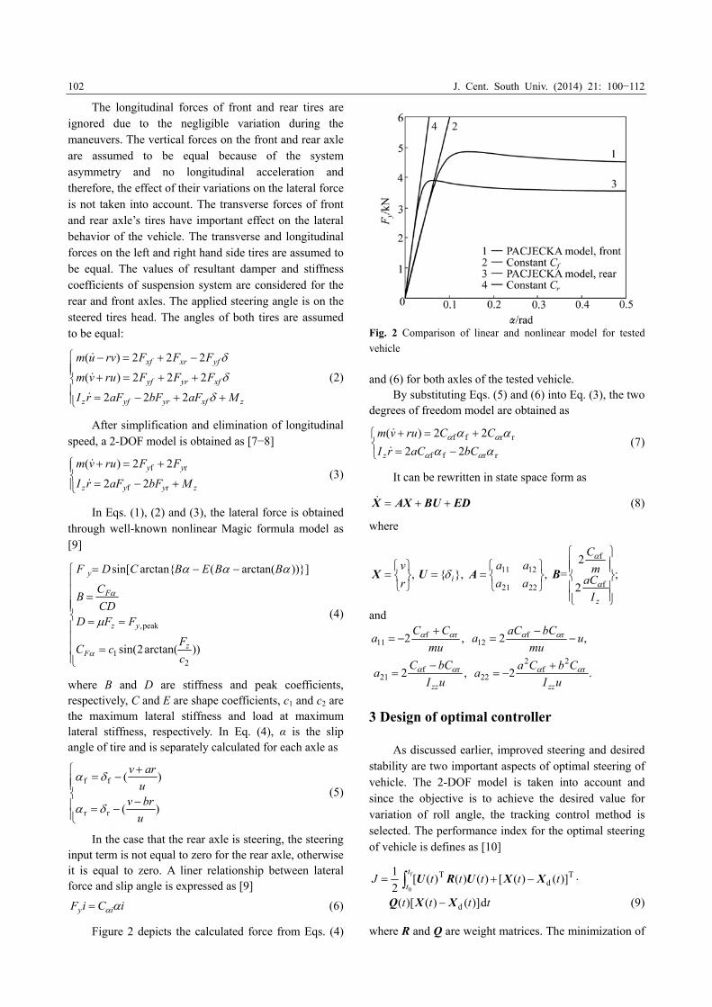
where B and D are stiffness and peak coefficients, respectively, C and E are shape coefficients, c1 and c2 are the maximum lateral stiffness and load at maximum lateral stiffness, respectively. In Eq. (4), α is the slip angle of tire and is separately calculated for each axle as

)(

)(

rr

ff

u

brvu

arv

(5)

In the case that the rear axle is steering, the steering

input term is not equal to zero for the rear axle, otherwise it is equal to zero. A liner relationship between lateral force and slip angle is expressed as [9]

iCiF iy (6)

Figure 2 depicts the calculated force from Eqs. (4)

Fig. 2 Comparison of linear and nonlinear model for tested

vehicle

and (6) for both axles of the tested vehicle. By substituting Eqs. (5) and (6) into Eq. (3), the two

degrees of freedom model are obtained as

rrff

rrff

22

22)(

bCaCrI

CCruvm

z

(7)

It can be rewritten in state space form as

EDBUAXX (8)

where

,

r

vX },{ iU ,

2221

1211

aa

aaA B= ;

2

2

f

f

zI

aCm

C

and

,2 rf11 mu

CCa

,2 rf12 u

mu

bCaCa

,2 rf21 uI

bCCa

zz

.2 r

2f

2

22 uI

CbCaa

zz

3 Design of optimal controller

As discussed earlier, improved steering and desired stability are two important aspects of optimal steering of vehicle. The 2-DOF model is taken into account and since the objective is to achieve the desired value for variation of roll angle, the tracking control method is selected. The performance index for the optimal steering of vehicle is defines as [10]

f

0

Td

T )]()([)()()([2

1 t

ttttttJ XXURU

tttt d)]()()[( ]dXXQ (9) where R and Q are weight matrices. The minimization of

J. Cent. South Univ. (2014) 21: 100−112

103

performance index is performed in order to optimize the steering behavior of vehicle. By desired choosing of weight factors (Eq. (6)) and proper design of control law, the favorable values of roll angle variations and optimal steering are obtained and the dynamical constraints of vehicle are met. The Hamilton’s function is obtained from Eq. (9) as

)()(2

1

2

1)( d

Td

T XXQXXRUUuH

)( cT BAXP (10)

The state equations are written and according to the

constraints and boundary conditions, the algebraic nonlinear system of equations is obtained. The time related to the transient part of the system answer is very short, thus this system is studied in stable conditions:

0)(

0

dcT1T

T1T

QXBSBBRA

BBRAQA

K

KKKK (11)

The equations of above system are solved in three

ways including solution of differential equations, solution of ricatti equation using matrix reference model and solution of ricatti equation using adaptive matrix reference model:

)(T1c SXBR K (12)

The desired steering during turning and standard

maneuvers (like Lane change) is not achieved with zero roll angle, but in order to design the controller for 2-DOF model, it is assumed that when vehicle is moving with constant longitudinal speed during a turn with constant radius of R, the desired value of is defined as [11]

)21)(( us

desdukba

ur

(13)

In fact, the desired value of system state is determined as

dd

0

rX (14)

Since some of the system states cannot be measured

and they are effective in determination of controller output, these variables should be extracted. Hence, an estimator is needed in a control system. In this work, the lateral and longitudinal speed states which are required for determination of inputs to the optimal controller are extracted by simple estimation method. In order to estimate u and v by using longitudinal acceleration sensors, the acceleration of roll rate is obtained through the following estimator [12−13]:

m

m

m

m

ˆ

ˆ

0

0ˆ

ˆ

d

d

y

x

a

a

v

u

r

r

v

u

t

(15)

where axm, aym and rm are measured values of longitudinal acceleration, lateral acceleration and roll rate, respectively. u and v are the estimated values of longitudinal and lateral speed.

Accurate vehicle state estimation is necessary for the control algorithm. Because of environmental disturbances and high measuring cost on the production vehicles, some states, like the lateral velocity, cannot be measured directly through automotive sensors. An observer plays a crucial rule in controller design. In this work, the scale method is used [3, 14−16]. A schematic of complete control system is illustrated in Fig. 3.

Fig. 3 Schematic of control system

J. Cent. South Univ. (2014) 21: 100−112

104

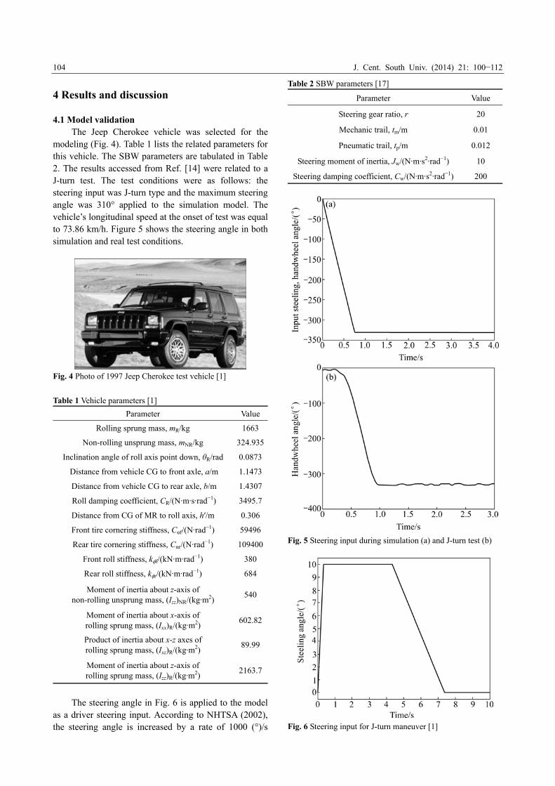
4 Results and discussion 4.1 Model validation

The Jeep Cherokee vehicle was selected for the modeling (Fig. 4). Table 1 lists the related parameters for this vehicle. The SBW parameters are tabulated in Table 2. The results accessed from Ref. [14] were related to a J-turn test. The test conditions were as follows: the steering input was J-turn type and the maximum steering angle was 310° applied to the simulation model. The vehicle’s longitudinal speed at the onset of test was equal to 73.86 km/h. Figure 5 shows the steering angle in both simulation and real test conditions.

Fig. 4 Photo of 1997 Jeep Cherokee test vehicle [1]

Table 1 Vehicle parameters [1]

ValueParameter

1663 Rolling sprung mass, mR/kg

324.935Non-rolling unsprung mass, mNR/kg

0.0873Inclination angle of roll axis point down, θR/rad

1.1473 Distance from vehicle CG to front axle, a/m

1.4307 Distance from vehicle CG to rear axle, b/m

3495.7 Roll damping coefficient, CR/(N·m·s·rad−1)

0.306Distance from CG of MR to roll axis, h′/m

59496Front tire cornering stiffness, Cαf/(N·rad−1)

109400Rear tire cornering stiffness, Cαr/(N·rad−1)

380 Front roll stiffness, kf/(kN·m·rad−1)

684 Rear roll stiffness, kr/(kN·m·rad−1)

540 Moment of inertia about z-axis of

non-rolling unsprung mass, (Izz)NR/(kg·m2)

602.82Moment of inertia about x-axis of rolling sprung mass, (Ixx)R/(kg·m2)

89.99Product of inertia about x-z axes of rolling sprung mass, (Ixz)R/(kg·m2)

2163.7Moment of inertia about z-axis of rolling sprung mass, (Izz)R/(kg·m2)

The steering angle in Fig. 6 is applied to the model as a driver steering input. According to NHTSA (2002), the steering angle is increased by a rate of 1000 (°)/s

Table 2 SBW parameters [17]

Value Parameter

20 Steering gear ratio, r

0.01 Mechanic trail, tm/m

0.012 Pneumatic trail, tp/m

10 Steering moment of inertia, Jw/(N·m·s2·rad−1)

200 Steering damping coefficient, Cw/(N·m·s2·rad−1)

Fig. 5 Steering input during simulation (a) and J-turn test (b)

Fig. 6 Steering input for J-turn maneuver [1]

J. Cent. South Univ. (2014) 21: 100−112

105

until it reaches 8 times of the dstat value, where dstat is the steering angle which is necessary to achieve a 0.3g lateral acceleration.

Actually, the input of this test was extracted according to the United States National Highway Traffic Safety Administration’s (NHTSA) and Vehicle Research and Test Center (VRTC). The steering input was applied with 0.5 s delay in the real test, thus the real model outputs have the same time delay as this value. The results obtained show that the nonlinear 4-DOF model gives the same lateral acceleration as the measured one (Fig. 7).

Fig. 7 Curves of simulated lateral acceleration (a) and lateral

acceleration of real test (b) [14]

Figure 8 illustrates that the roll angle has reached to

the maximum of 6° in the real test which is compatible with simulation results. After validating the nonlinear model, the compatibility of two-degree of freedom model to the more complete model should be evaluated. The standard sinusoidal test was used for simulation and designing of the controller. The test speed was 80 km/h or 22.2 m/s. The steering amplitude of tires was 3° and the variation frequency was 0.5 Hz. Figure 8 depicts that both 2° and 4° of freedom models are in good agreement.

Fig. 8 Roll angle of simulation (a) and real test (b) [14]

4.2 Controller design

Firstly, the weight coefficients for the optimal design of controller should be selected and then the ratios of Q22 to R and Q22 to Q11 were selected and evaluated. The simulation results indicate that the best choice for final controller design is achieved as

]1[2221

1211

R

QQQ

QQ

(16)

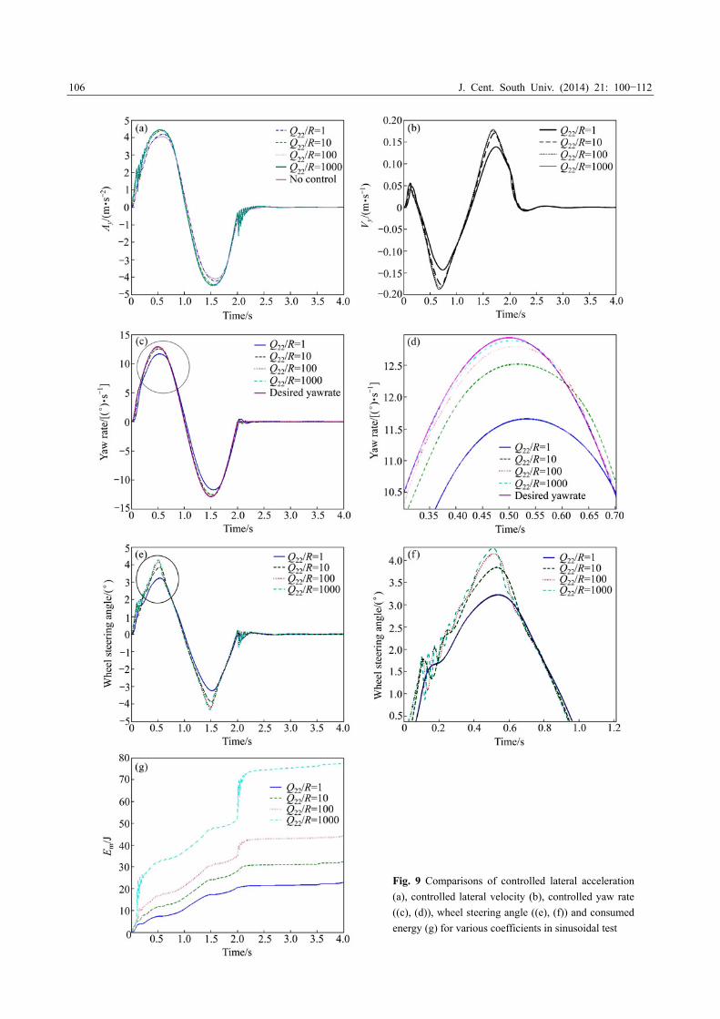
Figures 9(a) and (b) show the comparison of

controlled lateral acceleration and velocity with various coefficients in sinusoidal test, respectively. As can be seen, the lateral velocity is much lower than that of the first coefficient, but it will not have a positive influence on the next diagram.

The values of controlled yaw rate with various coefficients in sinusoidal test are depicted in Figs. 9(c) and (d). The comparison of controlled wheel steering angle with various coefficients in sinusoidal test is shown in Figs. 9(e) and (f). It is obvious that the values of Q22/R=100 and Q22/R=1000 are very close to desired values. By increasing Q22, the control costs are increased and therefore higher control steering angle is applied.

J. Cent. South Univ. (2014) 21: 100−112

106

Fig. 9 Comparisons of controlled lateral acceleration

(a), controlled lateral velocity (b), controlled yaw rate

((c), (d)), wheel steering angle ((e), (f)) and consumed

energy (g) for various coefficients in sinusoidal test

J. Cent. South Univ. (2014) 21: 100−112

107

Hence, energy consumption diagrams of the controller should be examined. Figure 9(g) shows the consumed energy by the SBW motor.

It can be observed that the energy consumption of the system is related to Q22/R ratio. It can be concluded that the coefficient of 100 is more appropriate for achieving good performance of the SBW system with lower energy consumption.

One of important ways of ensuring the selection of most appropriate coefficient is the studying of lateral forces on the tires during the maneuver (Figs. 10 and 11). As can be seen in Fig. 10, the maximum force for one of front (Fyf) and rear axle tires (Fyt) are 2700 and 2170 N, respectively. It is evident from Figs. 11(a) and (b) that the lateral force is close to the tire maximum force for both coefficients. On the other hand, it is very consistent for both coefficients. Therefore, Q22/R=1000 with higher energy consumption does not have much difference from previous coefficient and hence Q22/R=100 would be the best choice. Figure 11(c) shows the lateral force of rear axle which confirms this issue.

Fig. 10 Force versus tire side slip in wet asphalt road condition

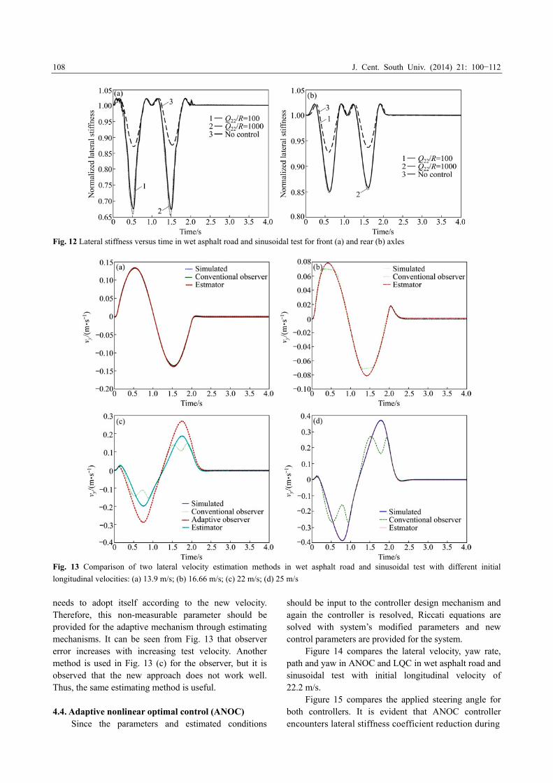
Figure 12 depicts the variation of normalized lateral

stiffness with time. As can be seen, there are severe variations which are not taken into account during the controller design.

Fig. 11 Force versus time in wet asphalt road and sinusoidal

test for front axle ((a), (b)) and rear axle (c)

4.3 Parameter estimating

Figure 13 shows that the lateral velocity is a parameter with large variations which should be available for controller updating and matching under road conditions. Thus, it should be estimated from the system and be provided for the adaptive mechanism. On the other hand, one of the system states required for controller design is the longitudinal velocity. In the initial steps of controller design, it is assumed to be constant. However, at each time the vehicle controller wants to make a decision in various velocity conditions, and it

J. Cent. South Univ. (2014) 21: 100−112

108

Fig. 12 Lateral stiffness versus time in wet asphalt road and sinusoidal test for front (a) and rear (b) axles

Fig. 13 Comparison of two lateral velocity estimation methods in wet asphalt road and sinusoidal test with different initial

longitudinal velocities: (a) 13.9 m/s; (b) 16.66 m/s; (c) 22 m/s; (d) 25 m/s

needs to adopt itself according to the new velocity. Therefore, this non-measurable parameter should be provided for the adaptive mechanism through estimating mechanisms. It can be seen from Fig. 13 that observer error increases with increasing test velocity. Another method is used in Fig. 13 (c) for the observer, but it is observed that the new approach does not work well. Thus, the same estimating method is useful. 4.4. Adaptive nonlinear optimal control (ANOC)

Since the parameters and estimated conditions

should be input to the controller design mechanism and again the controller is resolved, Riccati equations are solved with system’s modified parameters and new control parameters are provided for the system.

Figure 14 compares the lateral velocity, yaw rate, path and yaw in ANOC and LQC in wet asphalt road and sinusoidal test with initial longitudinal velocity of 22.2 m/s.

Figure 15 compares the applied steering angle for both controllers. It is evident that ANOC controller encounters lateral stiffness coefficient reduction during

J. Cent. South Univ. (2014) 21: 100−112

109

Fig. 14 Comparison of lateral velocity (a), yaw rate (b), path (c) and yaw (d) in ANOC and LQC in wet asphalt road and sinusoidal

test with initial longitudinal velocity of 22.2 m/s

Fig. 15 Comparison of steering angle of ANOC with LQC

methods in wet asphalt road and sinusoidal test with initial

longitudinal velocity of 22.2 m/s

the test, it adopts itself with the conditions and applies lower steering angle and it can guide the vehicle well. 4.5 Snowy road test

In order to seriously examine, the model equipped with controller undergoes a tougher test (snowy road test). In this condition, the vehicle without control does not follow the desired lane and also its stability is drawn

out of way. It is clear in Fig. 16 that the vehicle without controller has unstable performance and the designed controller controls it well. The results in Fig. 16 show that the optimal controller with estimator can effectively make the vehicle stable under snowy road conditions and prevent it from any accident. 4.6 Modeling by HIL

Due to the lack of experimental facilities for testing a real vehicle equipped with the considered controller, the HIL method is used for modeling. In this work, an ECU is designed and manufactured using Atmega16 microcontroller from AVR family. It is connected to a computer through serial port. The vehicle model is simulated in the computer and the output values of the system are transmitted to the ECU through the serial port as model sensor outputs. The ECU circuit acts as controller by receiving information from the system, and creates the modified steering angle by using linear optimal control method and estimation of lateral speed. This modified steering angle is returned to the simulated system as an input and forms a closed control loop. The Simulink MATLAB is used for the simulation and CodeVision is used for the coding of microprocessor, as shown in Fig. 17.

J. Cent. South Univ. (2014) 21: 100−112

110

Fig. 16 Comparisons of controlled and uncontrolled vehicle in snowy road and sinusoidal maneuver with initial longitudinal velocity

of 22.2 m/s: (a) Lateral velocity; (b) Yaw rate; (c) Lateral acceleration; (d) Path; (e) Yaw; (e) Modified steering wheel angle

Fig. 17 Hardware loop and its components

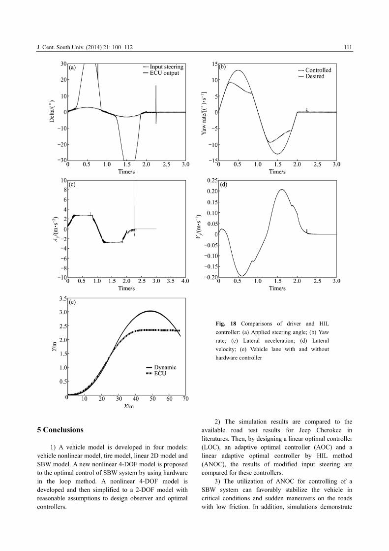
Then, the controller is exited from simulation mode and the output values of hardware controller are input to the system. This hardware controller gets the same simulated controller inputs through RS232 cable and after processing, returns it to simulated dynamical system. The hardware in the loop simulation indicates that the considered hardware can immediately calculate the control method and apply it to the vehicle. Figure 18 illustrates the comparison of driver and HIL controller on the steering, yaw rate, lateral acceleration and lateral velocity. It is assumed that the vehicle moves with constant speed of 80 km/h under snowy road condition.

J. Cent. South Univ. (2014) 21: 100−112

111

5 Conclusions

1) A vehicle model is developed in four models: vehicle nonlinear model, tire model, linear 2D model and SBW model. A new nonlinear 4-DOF model is proposed to the optimal control of SBW system by using hardware in the loop method. A nonlinear 4-DOF model is developed and then simplified to a 2-DOF model with reasonable assumptions to design observer and optimal controllers.

2) The simulation results are compared to the available road test results for Jeep Cherokee in literatures. Then, by designing a linear optimal controller (LOC), an adaptive optimal controller (AOC) and a linear adaptive optimal controller by HIL method (ANOC), the results of modified input steering are compared for these controllers.

3) The utilization of ANOC for controlling of a SBW system can favorably stabilize the vehicle in critical conditions and sudden maneuvers on the roads with low friction. In addition, simulations demonstrate

Fig. 18 Comparisons of driver and HIL

controller: (a) Applied steering angle; (b) Yaw

rate; (c) Lateral acceleration; (d) Lateral

velocity; (e) Vehicle lane with and without

hardware controller

J. Cent. South Univ. (2014) 21: 100−112

112

that the proposed controller can considerably improve vehicle handling during a severe maneuver. References [1] KAZEMI R, JANBAKHSH A A. Nonlinear adaptive sliding mode

control for vehicle handling improvement via steer-by-wire [J].

International Journal of Automotive Technology, 2010, 11(3):

345−354.

[2] YAO Y. Vehicle steer-by-wire system control [J]. SAE Technical

Paper Series, 2006, DOI: 10.4271/2006-01-1175.

[3] YIH P. Steer-by-wire: Implications for vehicle handling and safety

[D]. Stanford: Stanford University, 2005.

[4] QIU X, YU M, ZHANG Z, RUAN J. Research on steering control

and simulation of vehicle steer-by-wire system [C]// 7th International

Conference on MEMS, NANO and Smart Systems, ICMENS 2011.

Kuala Lumpur, 2011: 403−408.

[5] MARUMO Y A, KATAGIRI N. Control effects of steer-by-wire

system for motorcycles on lane-keeping performance [J]. Vehicle

System Dynamics, 2011, 49(8): 1283−1298.

[6] SALAAMI M K, GUENTHER D A, HEYDINGER G J. Vehicle

dynamics modeling for the national advanced driving simulator of a

1997 jeep cherokee [J]. SAE Paper, 1999, DOI: 104271/1999-01-

0121.

[7] RAJMANI R. Vehicle dynamic and control [M]. New York: Springer,

2006: 467−471.

[8] WONG J Y. Theory of ground vehicles [M]. USA: John Wiley &

Sons, Inc, 2001: 30−72.

[9] PACEJKA H B. Tyre and vehicle dynamics [M]. Oxford: Butterworth

Heinemann, 2002: 90−155.

[10] KIRK E. Optimal control theory: An introduction [M]. Englewood

Cliffs: Prentice-hall, Inc, 1970: 53−309.

[11] ESMAILZADEH E, GOODARZI A, VOSSOUGHI G R. Optimal

yaw moment control law for improved vehicle handling [J]. Int J

Mechatronics, 2003, 13: 659−675.

[12] SLOTINE J J, LI W. Applied nonlinear control [M]. 1st ed.

Englewood Cliffs: Prentice Hall International Inc, 1992: 311−388.

[13] BAYANI M. Designing vehicle stabilizer controller estimator [D].

Tehran: Mechanic Engineering Department, K. N. Toosi University

of Technology, 2007. (in Persian)

[14] NHTSA. A comprehensive evaluation of test maneuver that may

include on-road, untripped, light vehicle rollover [R]. Washington

DC: National Highway Traffic Safety Administration, 2002.

[15] CHEN B C, PENG H. Differential-braking-based rollover prevention

for sport utility vehicles with human-in-the-loop evaluations [J].

Vehicle System Dynamics, 2001, 36(4/5): 359−389.

[16] BROGAN W L. Modern control theory [M]. Englewood Cliffs:

Prentice-hall, 1991: 373−383.

[17] CHANG S C. Synchronization in a steer-by-wire vehicle dynamic

system [J]. International Journal of Engineering Science, 2007, 45:

628−643.

(Edited by FANG Jing-hua)