Ethernet in Steer-by-wire Applications - KTH
155
Degree project in Communication Systems Second level, 30.0 HEC Stockholm, Sweden MUHAMMAD IBRAHIM Ethernet in Steer-by-wire Applications KTH Information and Communication Technology
Transcript of Ethernet in Steer-by-wire Applications - KTH

Degree project inCommunication Systems
Second level, 30.0 HECStockholm, Sweden
M U H A M M A D I B R A H I M
Ethernet in Steer-by-wire Applications
K T H I n f o r m a t i o n a n d
C o m m u n i c a t i o n T e c h n o l o g y

Ethernet in Steer-by-wire Applications
Muhammad Ibrahim [email protected]
July 18, 2011
Supervisors
Prof. Gerald Maguire Kungliga Tekniska
Högskolan
Marco Monzani Cpac Systems AB
Jonas Lext Time Critical Networks AB
KTH Royal Institute of Technology School of Information and Communication Technology
Stockholm, Sweden


i
Abstract
A Controller Area Network (CAN) is a multi-master serial data communication bus designed primarily for the automotive industry. It is reliable and cost-effective and features error detection and fault confinement capabilities. CAN has been widely used in other applications, such as onboard trains, ships, construction vehicles, and aircraft. CAN has even been applied within the industrial automation segment in a range of devices such as programmable controllers, industrial robots, digital and analog I/O modules, sensors, etc.
Despite its robustness and other positive features, the CAN bus has limitations in form of limited maximum data rate and maximum bus length. Also the CAN network topology is rigidly fixed which is a severe limiting factor in some of its application cases, therefore several industrial actors are evaluating alternatives to CAN.
Ethernet is one of the potential candidates to replace CAN. It is a widespread and well known technology, easily accessible, and many off-the-shelf solutions are available. It can support extended networks and offers wide possibilities in terms of network topology thanks to active switches. It features very high bandwidth, which has increased systematically from 10 Mbps to 100 Gbps year after year, always preserving backward compatibility to the maximum possible extent.
The purpose of this thesis project is to investigate the possibility of replacing the CAN bus with Ethernet according to the following requirements:
• Standard off-the-shelf components and software stacks • No modification of the network node application software, i.e. messages formatted according
to CAN protocols must be transferred by means of Ethernet
A main issue is that CAN is time deterministic; it is always possible to predict the maximum latency in a message transfer. On the other hand Ethernet is still considered unreliable for time-critical applications, although the advent of Ethernet switches has minimized this non-deterministic behavior
A unique approach to this issue is offered as a result of the work done by Time Critical Networks, a newly started Swedish company. Their tool makes it possible to calculate the maximum forwarding time of a frame in an Ethernet network. This tool may make it possible to validate the use of Ethernet for time-critical applications.
CPAC Systems, a company in the Volvo group which develops and manufactures steer-by-wire systems based on the CAN technology, wishes to verify whether Ethernet could now be considered as a solution to complement or replace CAN, thus overcoming CAN’s limitations. This verification is the goal of this master thesis project.
The work was carried out through three different phase:
• First we performed a theoretical evaluation by modeling the Ethernet network using Time Critical Network’s tools.
• Next we verified the results by implementing the modeled CAN/Ethernet network that was previously modeled.
• Finally, we validated the solution by directly testing the modeled CAN/Ethernet in combination with CPAC System’s steer-by-wire technology.
The results obtained show that Ethernet in combination with Time Critical Network’s modeling tool, when it comes to time-determinism, can be a complement and/or an alternative to the CAN bus.


iii
Sammanfattning
En Controller Area Network (CAN) är en multi-master seriell datakommunikation buss utformad främst för fordonsindustrin. Den är pålitlig och kostnadseffektiv och har feldetektering och fel förmåga instängdhet. CAN har ofta används i andra tillämpningar, som ombord på tåg, fartyg, fordon konstruktion, och flygplan. CAN har även använts inom industriautomation segmentet i en rad apparater som programmerbara styrsystem, industrirobotar, digitala och analoga I / O-moduler, sensorer, etc.
Trots sin robusthet och andra positiva egenskaper har CAN-bus begränsningar i form av begränsad maximal datahastighet och maximal buss längd. Även CAN nätverkstopologin är fast förankrade vilket är en svår begränsande faktor i några av dess tillämpning fall därför flera industriella aktörer utvärderar alternativ till CAN.
Ethernet är en av de potentiella sökande för att ersätta CAN. Det är en utbredd och väl känd teknik, lättillgänglig, och många off-the-shelf lösningar finns tillgängliga. Det kan stödja utökade nätverk och erbjuder stora möjligheter när det gäller nätverkstopologin tack vare aktiv växlar. Den har mycket hög bandbredd, vilket har ökat systematiskt från 10 Mbps till 100 Gbps år efter år, alltid bevara bakåtkompatibilitet i största möjliga utsträckning.
Syftet med detta examensarbete är att undersöka möjligheten att ersätta CAN-bussen med Ethernet i enlighet med följande krav:
• Standard off-the-shelf komponenter och stackar programvara • Inga ändringar av nätverket nod programvara, formaterade dvs meddelanden enligt CAN-
protokoll måste överföras med hjälp av Ethernet
En viktig fråga är att CAN är dags deterministisk, det är alltid möjligt att förutse den maximala fördröjning i ett överfört meddelande. Å andra sidan Ethernet är fortfarande betraktas som otillförlitliga för tidskritiska applikationer, även om tillkomsten av Ethernet-switchar har minimerat denna icke-deterministiska beteende
En unik inställning till denna fråga är erbjuds som ett resultat av det arbete som tidskritiska Networks, ett nystartat svenskt företag. Deras verktyg gör det möjligt att beräkna den maximala vidarebefordran tid för en ram i ett Ethernet-nätverk. Detta verktyg kan göra det möjligt att validera användningen av Ethernet för tidskritiska applikationer.
CPAC Systems, ett bolag inom Volvokoncernen som utvecklar och tillverkar styr-by-wire-system baserade på CAN-tekniken, vill kontrollera om Ethernet nu kan betraktas som en lösning för att komplettera eller ersätta kan således övervinna CAN: s begränsningar. Denna kontroll är målet för detta examensarbete.
Arbetet genomfördes genom tre olika fas:
• Först utförs en teoretisk utvärdering av modellering Ethernet-nätverk med hjälp av tidskritiska Networks verktyg.
• Nästa vi verifierat resultat genom att genomföra de modellerade CAN / Ethernet-nätverk som tidigare modellerats.
• Slutligen, validerade vi lösningen genom att direkt testa de modellerade CAN / Ethernet i kombination med CPAC Systems steer-by-wire-teknik.
De resultat som erhållits visar att Ethernet i kombination med tidskritiska Networks modelleringsverktyg, när det gäller tid-determinism, kan vara ett komplement och / eller ett alternativ till CAN-bussen.


v
Acknowledgements
First and foremost I would like to thank God for giving me the opportunity, strength and health to do this thesis project without any difficulties. I would like to express my sincere gratitude to my industrial supervisor at CPAC Systems, Marco Monzani, who offered me this master thesis project, whose encouragement, supervision and support from the beginning to the end at every level enabled me to develop the understanding of the work and finish the project successfully. I am extremely thankful to my second industrial supervisor at Time Critical Networks, Jonas Lext, for assisting me to use their software and modeling tool and for the fruitful discussions regarding the thesis project. I would like to express my thanks to my academic supervisor and examiner at KTH, Prof. Gerald Q. Maguire Jr., for providing me valuable reviews and suggestions to improve the thesis project and the report. Furthermore, good wishes and warm regards to my family (specially my mother) for their unwavering support during my entire master studies. Lastly, I want to dedicate this master thesis to my late father the source of inspiration for me to choose engineering as a career.


Contents
vii
Contents
Abstract ............................................................................................................................................ i Sammanfattning ............................................................................................................................. iii Acknowledgements .......................................................................................................................... v Contents ......................................................................................................................................... vii List of Figures ................................................................................................................................. xi List of Tables ................................................................................................................................. xv Acronyms and Abbreviations ...................................................................................................... xvii 1 Introduction ............................................................................................................. 2
1.1 Background ............................................................................................................................ 2 1.2 Thesis research area ................................................................................................................ 3 1.3 Purpose of the research ........................................................................................................... 4 1.4 Research methodology............................................................................................................ 5
1.4.1 Theoretical evaluation ................................................................................................ 5 1.4.2 Practical verification .................................................................................................. 5 1.4.3 Validation on test rigs ................................................................................................ 6
1.5 Report structure ...................................................................................................................... 6 2 Background .............................................................................................................. 7
2.1 Network Architecture ............................................................................................................. 7 2.1.1 Physical Layer ........................................................................................................... 8 2.1.2 Data Link Layer ......................................................................................................... 8 2.1.3 Network Layer ........................................................................................................... 9 2.1.4 Transport Layer ......................................................................................................... 9 2.1.5 Session Layer ............................................................................................................. 9 2.1.6 Presentation Layer ..................................................................................................... 9 2.1.7 Application Layer ...................................................................................................... 9
2.2 Controller Area Network ...................................................................................................... 10 2.2.1 Protocol overview .................................................................................................... 10 2.2.2 CAN bus topology drawbacks .................................................................................. 13 2.2.3 CAN Controller ....................................................................................................... 13 2.2.4 CAN Higher Layer Protocols ................................................................................... 14
2.3 Ethernet ................................................................................................................................ 16 2.4 IEEE 802.3 ........................................................................................................................... 17 2.5 TCP/IP - Network Protocol Stack ......................................................................................... 19
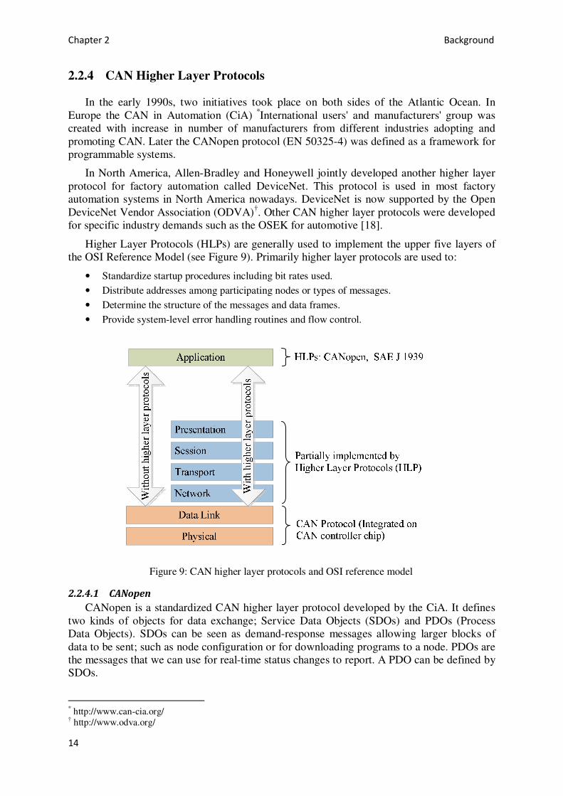
2.5.1 Internet Protocol (IP) ............................................................................................... 20 1.1.1. Address Resolution Protocol (ARP) ......................................................................... 21 2.5.2 Internet Control Message Protocol (ICMP)............................................................... 21 2.5.3 Dynamic Host Configuration Protocol (DHCP) ........................................................ 21 2.5.4 Transmission Control Protocol (TCP)....................................................................... 22 2.5.5 User Datagram Protocol (UDP) ................................................................................ 22
2.6 TCP/IP stack for CAN/Ethernet converter............................................................................. 23 2.6.1 LwIP - A Lightweight TCP/IP stack ......................................................................... 24 2.6.2 Interfacing with the Stack......................................................................................... 28
2.7 Ethernet Switch .................................................................................................................... 29 2.7.1 Cut-Through vs. Store-and-Forward ......................................................................... 29 2.7.2 Data Flow Model ..................................................................................................... 29

Contents
viii
2.7.3 Virtual LAN............................................................................................................. 31 2.8 Latency in a switched Ethernet network ................................................................................ 32
2.8.1 Sources of Latency ................................................................................................... 33 2.8.2 Total Worst-Case Latency Calculation (������) ................................................... 35 2.8.3 TCN Analyzer and Latency in Ethernet network....................................................... 35
2.9 TCN Analyzer ...................................................................................................................... 36 2.9.1 Computational Engine .............................................................................................. 36 2.9.2 Switch modeling ...................................................................................................... 36 2.9.3 Transmission medium modeling ............................................................................... 36 2.9.4 Frame modeling ....................................................................................................... 37 2.9.5 Flow modeling ......................................................................................................... 37 2.9.6 Performing the analysis ............................................................................................ 38
2.10 Prior work ............................................................................................................................ 38 2.10.1 Realization on top of TCP/IP protocols .................................................................... 39 2.10.2 Realization on top of Ethernet .................................................................................. 40 2.10.3 Realization with modified Ethernet .......................................................................... 40 2.10.4 Realization with cots switches .................................................................................. 41 2.10.5 Numerical simulation and practical verification ........................................................ 41
3 Method ................................................................................................................... 43 3.1 Introduction .......................................................................................................................... 43 3.2 Theoretical evaluation / simulation ....................................................................................... 43
3.2.1 Westermo RedFox switch ........................................................................................ 43 3.2.2 Network model ........................................................................................................ 44
3.3 Practical evaluation / verification .......................................................................................... 47 3.3.1 Achieving TCN Analyzer upper bound..................................................................... 47 3.3.2 Preliminary proposal limitations ............................................................................... 50 3.3.3 Click-Sink................................................................................................................ 51 3.3.4 CAN/Ethernet Converter .......................................................................................... 52
3.4 CAN/Ethernet Converter Application layer ........................................................................... 58 3.4.1 Porting LwIP to STM32F107VC .............................................................................. 59 3.4.2 Application layer firmware....................................................................................... 62 3.4.3 CAN/Ethernet converter as UDP traffic generator .................................................... 63
3.5 Net analyzer ......................................................................................................................... 64 3.5.1 Connecting the analyzer card to capture traffic ......................................................... 65 3.5.2 Time-stamps ............................................................................................................ 65 3.5.3 Graphical User Interfaces ......................................................................................... 66
3.6 PCAN-USB .......................................................................................................................... 67 3.7 Network setups ..................................................................................................................... 67
3.7.1 Single flow .............................................................................................................. 68 3.7.2 Two flows ................................................................................................................ 70 3.7.3 Four flows ............................................................................................................... 72 3.7.4 Seven flows ............................................................................................................. 74
3.8 CAN/Ethernet conversion time ............................................................................................. 75 3.9 Validation on the test rigs ..................................................................................................... 76
3.9.1 Single driveline ........................................................................................................ 77 3.9.2 Twin driveline.......................................................................................................... 79
4 Analysis .................................................................................................................. 81 4.1 Theoretical evaluation: modeling and simulation .................................................................. 81

Contents
ix
4.2 Practical evaluation / verification .......................................................................................... 83 4.3 netANALYZER serialization time problem .......................................................................... 84 4.4 Single flow ........................................................................................................................... 86 4.5 Seven flows .......................................................................................................................... 90 4.6 Forwarding time for all flows ............................................................................................... 94 4.7 Comparison: Theoretical vs. Practical ................................................................................... 96 4.8 CAN/Ethernet conversion time & end-to-end latency ............................................................ 98 4.9 Bandwidth utilization ......................................................................................................... 101 4.10 Validation results................................................................................................................ 103
5 Conclusions and Future Work............................................................................. 105 5.1 Summary ............................................................................................................................ 105 5.2 Learning ............................................................................................................................. 106 5.3 Conclusions ........................................................................................................................ 106 5.4 Future Work ....................................................................................................................... 106
Bibliography and references ....................................................................................................... 109 Appendix A: Stream Analyzer plots ........................................................................................... 115 Appendix B: (Compensated) Measured vs. TCN forwarding times .......................................... 130 Appendix C: Drawbacks of Click source .................................................................................... 132


List of Figures
xi
List of Figures
Figure 1: The basic network setup.................................................................................................. 6 Figure 2: OSI reference model for network communications .......................................................... 8 Figure 3: CAN and the OSI reference model ................................................................................ 10 Figure 4: CAN topology .............................................................................................................. 11 Figure 5: CAN differential bus..................................................................................................... 11 Figure 6: CAN message frame format .......................................................................................... 12 Figure 7: Relationship between bit rate and bus length ................................................................. 13 Figure 8: Typical CAN bus topology. .......................................................................................... 13 Figure 9: CAN higher layer protocols and OSI reference model ................................................... 14 Figure 10: Typical J1939 vehicle network ...................................................................................... 15 Figure 11: Ethernet frame format ................................................................................................... 16 Figure 12: IEEE802.3 in the OSI reference model .......................................................................... 18 Figure 13: Ethernet Point-to-Point topology ................................................................................... 18 Figure 14: Ethernet Star topology .................................................................................................. 19 Figure 15: TCP/IP suite of protocols .............................................................................................. 20 Figure 16: Encapsulation in the case of TCP/IP over Ethernet ........................................................ 21 Figure 17: UDP frame format ........................................................................................................ 23 Figure 18: A PBUF_RAM pbuf with data in memory managed by the pbuf subsystem. ................. 25 Figure 19: ICMP processing in LwIP TCP/IP stack ........................................................................ 27 Figure 20: UDP processing in LwIP TCP/IP stack ......................................................................... 28 Figure 21: Ethernet switch data flow in Store and Forward switch ................................................. 30 Figure 22: Graphical user interface of TCN Analyzer .................................................................... 38 Figure 23: Possible real-time Ethernet realizations ......................................................................... 39 Figure 24: One flow modeling in TCN Analyzer ............................................................................ 45 Figure 25: Four flows modeled in TCN Analyzer........................................................................... 46 Figure 26: Seven flows modeling in TCN Analyzer ....................................................................... 47 Figure 27: Perfect simultaneous arrival of Ethernet frames............................................................. 49 Figure 28: Click Sink; configuration of Click elements .................................................................. 51 Figure 29: CAN/Ethernet converter layered model ......................................................................... 52 Figure 30: STM32F107VC development kit from IAR .................................................................. 54 Figure 31: STM32F107VC Ethernet peripheral block diagram ....................................................... 55 Figure 32: STM32F107VC CAN interface module block diagram ................................................. 56 Figure 33: CAN message filtering and storage in STM32F107VC ................................................. 58 Figure 34: Flow chart of main program .......................................................................................... 63 Figure 35: Flow chart of application layer ...................................................................................... 64 Figure 36: netANALYZER card simultaneously sniffing two Ethernet links .................................. 65 Figure 37: Time-stamping in netANALYZER ............................................................................... 66 Figure 38: netANALYZER software (GUI) ................................................................................... 66 Figure 39: PCAN-USB GUI .......................................................................................................... 67 Figure 40: Ethernet network setup for the evaluation of one flow case ........................................... 69 Figure 41: Ethernet network setup for the evaluation of two flows case .......................................... 71 Figure 42: Ethernet network setup for the evaluation of four flows case ......................................... 73 Figure 43: Ethernet network setup for the evaluation of seven flows case ....................................... 75 Figure 44: Setup to calculate CAN/Ethernet conversion delay ........................................................ 76 Figure 45: CAN Nodes and Bus locations in a typical boat ............................................................ 77

List of Figures
xii
Figure 46: EVC Single engine installation with dual helm station ECU diagram (single helm installation)................................................................................................................... 78
Figure 47: EVC Single engine installation with dual helm station with CAN-Ethernet Converters .................................................................................................................... 78
Figure 48: EVC twin-engine installation ........................................................................................ 79 Figure 49: EVC twin-engine installation with CAN-Ethernet Converters ....................................... 80 Figure 50: Bar graph for TCN Analyzer projected worst case forwarding time ............................... 83 Figure 51: Serialization problem in netANALYZER ...................................................................... 86 Figure 52: Forwarding time plot for all critical frames for single flow case .................................... 87 Figure 53: Forwarding time distribution plot for all critical UDP frames for the case of one
flow .............................................................................................................................. 88 Figure 54: Forwarding time graph plotted at maximum forwarding time instant for the case of
a single flow ................................................................................................................. 88 Figure 55: Forwarding time graph plotted at maximum interarrival time instant for the case of
single flow .................................................................................................................... 89 Figure 56: TAP B all frames arrival graph plotted at the maximum forwarding time instant for
the case of single flow .................................................................................................. 90 Figure 57: TAP B all frames arrival graph plotted at maximum interarrival time instant for the
case of single flow ........................................................................................................ 90 Figure 58: Forwarding time plot for all critical frames for the case of seven flows ......................... 91 Figure 59: Forwarding time distribution plot for all critical UDP frames for the case of seven
flows ............................................................................................................................ 91 Figure 60: Forwarding time graph plotted at maximum forwarding time instant for the case of
seven flows. .................................................................................................................. 92 Figure 61: Forwarding time graph plotted at maximum interarrival time instant for the case of
seven flows. .................................................................................................................. 93 Figure 62: TAP B all frames arrival graph plotted at the maximum forwarding time instant for
the case of seven flows. ................................................................................................ 93 Figure 63: TAP B all frames arrival graph plotted at the maximum interarrival time instant for
the case of seven flows. ................................................................................................ 94 Figure 64: Bar graph for (compensated) measured forwarding times .............................................. 95 Figure 65: Bar graph comparing TCN Analyzer projected and measured forwarding times of
64 bytes frame size flows. ............................................................................................. 96 Figure 66: Delays in the CAN/Ethernet conversion time measurement setup .................................. 98 Figure 67: End-to-End latency in CAN/Ethernet network ............................................................. 100 Figure 68: Stream Analyzer plots for single flow and 64 byte frame size setup ............................. 115 Figure 69: Stream Analyzer plots for single flow and 1514 byte frame size setup ......................... 116 Figure 70: Stream Analyzer plots for two flows and 64 byte frame size setup ............................... 117 Figure 71: Stream Analyzer plots for two flows and 1514 byte frame size setup ........................... 118 Figure 72: Stream Analyzer plots for two flows and 64 byte frame size setup ............................... 119 Figure 73: Stream Analyzer plots for three flows and 64 byte frame size setup ............................. 120 Figure 74: Stream Analyzer plots for three flows and 1514 byte frame size setup ......................... 121 Figure 75: Stream Analyzer plots for four flows and 64 byte frame size setup .............................. 122 Figure 76: Stream Analyzer plots for four flows and 1514 byte frame size setup .......................... 123 Figure 77: Stream Analyzer plots for five flows and 64 byte frame size setup .............................. 124 Figure 78: Stream Analyzer plots for five flows and 1514 byte frame size setup........................... 125 Figure 79: Stream Analyzer plots for six flows and 64 byte frame size setup ................................ 126 Figure 80: Stream Analyzer plots for six flows and 1514 byte frame size setup ............................ 127

List of Figures
xiii
Figure 81: Stream Analyzer plots for seven flows and 64 byte frame size setup ............................ 128 Figure 82: Stream Analyzer plots for seven flows and 1514 byte frame size setup ........................ 129 Figure 83: Bar graph comparing TCN Analyzer estimations and measured forwarding times of
64 bytes frame size flows. ........................................................................................... 130 Figure 84: TCN Analyzer estimations and (compensated) measured forwarding times of 514
bytes frame size flows. ................................................................................................ 130 Figure 85: TCN Analyzer estimations and (compensated) measured forwarding times of 1014
bytes frame size flows. ................................................................................................ 131 Figure 86: TCN Analyzer estimations and (compensated) measured forwarding times of 1514
bytes frame size flows. ................................................................................................ 131 Figure 87: Nondeterministic behavior of Click source. ................................................................. 133


List of Tables
xv
List of Tables
Table 1: In-service long ships ....................................................................................................... 4 Table 2: Practical CAN bus length at several bit rates ................................................................. 12 Table 3: Westermo RedFox RFI-10specifications ....................................................................... 44 Table 4: Memory Option Settings for LwIP ................................................................................ 60 Table 5: Pbuf Memory Options Configuration ............................................................................ 60 Table 6: IP Options Configuration Parameters ............................................................................ 60 Table 7: DHCP Options Configuration Parameters ..................................................................... 60 Table 8: ICMP Options Configuration Parameters ...................................................................... 60 Table 9: UDP Options Configuration Parameters ........................................................................ 60 Table 10: UDP Events, Callbacks, and Routine to register callback events .................................... 61 Table 11: Parameters set in CAN/Ethernet converter for one flow ................................................ 69 Table 12: Parameters set in CAN/Ethernet converter for two flows ............................................... 71 Table 13: Parameters set in CAN/Ethernet converter for four flows scenario ................................ 74 Table 14: Parameters set in CAN/Ethernet converter for four flows scenario ................................ 74 Table 15: TCN Analyzer projected worst case forwarding time .................................................... 82 Table 16: Measured forwarding times ........................................................................................... 94 Table 17: Compensated forwarding times ..................................................................................... 95 Table 18: Comparison of TCN Analyzer projected and (compensated) measured forwarding
times of 64 bytes frame size flows. ............................................................................... 96 Table 19: All forwarding times; TCN Analyzer projected and measured ....................................... 97 Table 20: TAP A and TAP B time-stamps .................................................................................... 99 Table 21: Worst case end-to-end latency in CAN/Ethernet network ............................................ 100 Table22: Bandwidth utilization with 1Mbps CAN bus speed ..................................................... 102 Table23: Bandwidth utilization with 250kbps CAN bus speed ................................................... 102 Table24: Bandwidth utilization with 125kbps CAN bus speed ................................................... 102 Table 25: CPAC Systems rigs tests results .................................................................................. 103


Acronyms and abbreviations
xvii
Acronyms and Abbreviations
ADC Analog to Digital Converter AFDX Avionics Full Duplex Switched Ethernet API Application Program Interface ARP Address Resolution Protocol BSD Berkeley Software Distribution bxCAN Basic extended CAN CAN Controller Area Network CEC CAN/Ethernet Converter CoS Class of Service COTS Commercial-off-the-shelf CRC Cyclic Redundancy Check CSMA/CD Carrier Sense Multiple Access / Collision Detection CSV Comma Separated Value CT Cut-Through DAC Digital to Analog Converter DHCP Dynamic Host Configuration Protocol DLC Data Length Code ECU Electronic Control Unit EOF End of Frame FCS Frame Check Sequence FDDI Fiber Distributed Data Interface FIFO First In First Out FTT-SE Flexible Time-Triggered Switch Ethernet GUI Graphical User Interface HCU Helm Control Station HLP Higher Layer Protocol HTTP Hypertext Transfer Protocol I/O Input/ Output I2C Inter-Integrated Circuit ICMP Internet Control Message Protocol IDE Identifier Extension IEEE Institute of Electrical and Electronics Engineers IGMP Internet Group Management Protocol IP Internet Protocol IRT Isochronous Real Time ISO International Organization for Standardization kbps Kilo bits per second LAN Local Area Network LIFO Last In First Out LLC Logical Link Control

Acronyms and abbreviations
xviii
LwIP Light Weight Internet Protocol MAC Medium Access Control MAN Metropolitan Area Network Mbps Mega bits per second MII Media-Independent Interface ms Milliseconds ns Nanoseconds OS Operating System
OSI Open Systems Interconnect PCB Protocol Control Block PCU Power Train Control Unit PPP Point-to-Point Protocol QoS Quality of Service RAM Random-access memory RFC Request for Comments RISC Reduced Instruction Set Computing RMII Reduced Media-Independent Interface ROM Read-only memory RSTP Rapid Spanning Tree Protocol RTPS Real-Time Publisher Subscriber SA Source Address SF Store-and-Forward SFD Start of Frame Delimiter SNMP Simple Network Management Protocol SOF Start of Frame SPI Serial Peripheral Interface TAP Test Access Point TCN Time Critical Networks TCP Transmission Control Protocol TFTP Trivial File Transfer Protocol UDP User Datagram Protocol µs Microseconds USART Universal Asynchronous Receiver/Transmitter VLAN Virtual Local Area Network VPID VLAN Protocol Identifier


1 http://www.cpacsystems.se 2 http://www.timecriticalnetworks.com
1 Introduction This master thesis project aims to evaluate Ethernet as a media to replace the Controller
Area Network (CAN) bus in a class of applications which is, as of today, based on such CAN technology. In particular this project investigates Ethernet as a communication medium in steer-by-wire systems for marine and industrial vehicles. The conclusions of this research will hopefully be used as a reference of marine industry to assist designers and architects of steer-by-wire systems in their decision of whether to replace CAN bus with Ethernet.
I carried out this master thesis project as part of the requirements to complete a Master of Science in Design and Implementation of Information and Communication Technology Products and Systems at the School of Information and Communication Technology, KTH Royal Institute of Technology in Stockholm, Sweden.
The content of this work was defined by CPAC Systems AB1, a Volvo company which develops and manufactures drive-by-wire and steer-by-wire systems for the marine industry and for industrial vehicles, within the more general framework of the CPAC Systems and Volvo Penta Advanced Engineering. The work was carried out in tight collaboration with Time Critical Networks AB2, another Swedish company that has developed a unique modeling method to assess the suitability of Ethernet networks when it comes to time-critical communication tasks.
In this chapter we briefly explain both Ethernet and Controller Area Network (section 1.1), the area of research (section 1.2), as well as the purpose of this research (section 1.3). Later we explain the methodology followed to carry out such research (section 1.4). Finally we outline the structure of the remaining sections of this report (section 1.5).
1.1 Background
Ethernet is a widespread computer networking technology for a number of reasons: high data rate, ability to communicate over relatively long distances, a natural choice when it comes to supporting well established and well known protocols such as TCP/IP, and the wide selection of cost-effective Commercial-Off-The-Shelf (COTS) hardware.
Ethernet is without a doubt the most widely installed local area network technology, being well suited for use in homes, offices, and even in certain industrial automation applications. It is easy to install and Ethernet interfaces are inexpensive. Numerous 8-bit microprocessors can communicate over Ethernet network via a built-in or off-chip Ethernet controller and Ethernet physical interface module [1]. Ethernet interfaces are also available as intellectual properly and can easily be added to custom integrated circuits.
Ethernet can transfer data frames of varying sizes, ranging from a minimum sized frame of 64 bytes to nearly 216 bytes. Today Ethernet is standardized by IEEE 802.3 [2]. Many variants are defined that can utilize different physical layers (including twisted copper pairs and optical fibers). Ethernet has evolved from a shared bus topology to a micro-segmented network (utilizing switches and point-to-point connections).
Ethernet can span long distances. A single twisted-pair cable between two Ethernet nodes communicating with each other can be up to 100 meters long. A half-duplex Ethernet link over fiber-optic medium at 10 Mbps can be as long as 2 kilometers, while 5 kilometers can be covered by using a full-duplex Ethernet network [3]. With repeater and switches a network can span even longer distances.

Chapter 1 Introduction
3
Improvements in bandwidth while maintaining backward compatibility gave Ethernet success in its wide deployment across various applications from office to industry, and from academia to home. Since its invention, Ethernet’s bandwidth has increased from 2.94 Mbps to 10 Mbps (DIX Ethernet II; 1980s), 100 Mbps (IEEE 802.3u; 1990s), 1 Gbps (IEEE 802.3z; 1998) [2], and 10 Gbps (IEEE 802.3ae; 2002). Last year the IEEE P802.3ba task force completed its working and published the standard IEEE Std 802.3ba-2010 for 40 Gbps and 100 Gbps Ethernet [4]. Increase in bandwidth and freedom in network scalability have made Ethernet (using special, non-COTS switches) a viable communication standard for extremely time critical and safety critical applications such as in the aviation industry for the exchange data between avionics systems (AFDX) [5].
However, during the early years of Ethernet development, the automotive industry had already developed its own types of network to support time-critical communication. In the mid 1980s, Robert Bosch GmbH introduced Controller Area Network (CAN) [6]; a multi-master network protocol. CAN is a high-integrity serial data communications bus designed to be reliable and cost-effective. It has excellent error detection and fault confinement capabilities.
Since its inception, the CAN protocol has gained widespread popularity in automotive applications. Though designed for automotive applications, CAN has been used in other types of vehicles too; from trains to ships and construction vehicles. Because of its fault tolerant properties, CAN has been adopted outside automotive applications, for example for industrial automation. A range of automation systems use CAN as a communication bus including programmable controllers, industrial robots, digital and analog I/O modules, sensors etc.
1.2 Thesis research area
CAN in vehicle industry is more or less the sole widespread standard for engine diagnostics and control. CAN is also used extensively for the implementation of most vehicle functions, with the exception of infotainment systems. Brakes, airbag, active steering, electronic stability, and even door locks are typically connected via CAN. In almost all cars, one CAN bus is dedicated to the engine and one to all other services. However, the vehicle industry has begun to look at alternatives due to the intrinsic limits of the CAN bus specifically the limited data rate (1 Mbps, see section 2.2.3) as well as drawbacks in terms of linear bus topology.
Despite bandwidth advantages, Ethernet has been perceived not being directly suitable for time-critical applications because of concerns regarding the latency of transmission of Ethernet data frames [7] [8]. In fact, this may be Ethernet’s key shortcoming: the actual time it takes for a packet to traverse the network is unpredictable [9]. This impedes its use in time- critical applications. In fact, the common Ethernet protocols can guarantee that a message is delivered from a node to another node within the same network, but cannot guarantee that this delivery will occur within a pre-defined period of time. The reasons behind unpredictability are varying latency, jitter, and frame loss/drop.
There are many reasons to replace CAN bus with other media. CAN is a relatively old technology with limitations in terms of bandwidth, maximum bus length, and network topology (CAN does not allow branching of the bus). The maximum data rate has become an issue with the increasing complexity of the functions and of the number of nodes that are connected together. The network topology as well as the maximum bus length become an issue when CAN is implemented onboard vehicles of very large size (such as ships and certain industrial vehicles). Another disadvantage of the CAN linear bus topology is its

Chapter 1 Introduction
4
weakness regarding single failures. A single failure in the main cable (such as a short circuit or open circuit) may cause a complete bus failure and consequently a failure of the whole network.
Ethernet might be the potential alternative to CAN because:
• Ethernet is a widespread technology, easily accessible, many ready-made solutions and relevant competence pools are available for the development.
• Ethernet can cover longer distances. • Ethernet offers wide possibilities in terms of topology because of its components such as the
active switches. • Ethernet features very high bandwidth (that has increased systematically from 10 Mbps to 100
Gbps with backward compatibility on the hardware level).
1.3 Purpose of the research
The control systems that CPAC Systems AB develops and manufactures are aimed at the marine industry. There are thus a number of reasons to question whether the CAN bus, which is used today, will be the correct technological choice in the future. CAN was intended to span relatively short distances (the distances being those typically found when wiring together vehicles’ Electronic Control Units (ECUs)). In contrast, the industry segment CPAC Systems is concerned with includes vessels of increasing size. Table 1 gives an overview of today’s in-service vessel sizes.
Table 1: In-service long ships [10]
Name Type Length (meters)
Maersk E-class Container 397.0
RMS Queen Mary 2 Ocean liner 345.0
AL Ghuwairiya LNG carrier 345.0
Berge Stahl Bulk cargo 343.0
MSC Fantasia Cruise 333.0
Engines from Volvo Penta can be found on vessels of sizes up to 30 meters as of today,
and plans are being made to improve the engines for installations in vessels of much larger size.
The major issues concerning bus selection are:
a) CAN is time-deterministic, while Ethernet is not. The philosophy behind the system architecture, including the safety analysis and from there the ECU software, were founded on the assumption of a time-deterministic bus, as CAN is. It is in principle not possible to switch to a non-time-deterministic bus without redesigning all of the software and, even more, a complete review of the safety strategy. In simple terms, a critical message travelling across the network must be delivered within a certain amount of time, which is deterministically known when the CAN bus is used (under the assumption that a number of criteria are fulfilled). When Ethernet is used, the delivery time of the message can be only defined statistically.
b) The cost of the complete hardware solution with specific reference to the wiring and the connectors. CAN makes the use of a simple twisted pair with cheap and reliable

Chapter 1 Introduction
5
connectors, suitable for rough environments, while the standard Ethernet requires more complex wiring and is typically based on a RJ-45 type connector, which is very weak from mechanical point of view, is rather quickly affected by humidity and saline mist, typical of the marine environment, and by vibrations, which are rather intense on-board most vehicles.
The purpose of this thesis project is to address point (a) by evaluating if Ethernet with COTS switches can be a viable replacement for CAN, or a complement to CAN, when it comes to large vehicles featuring functions of increasing complexity. The idea is to verify whether standard Ethernet can be an appropriate solution without doing a complete review of the function deployment strategy (i.e., the way to distribute functions across CAN nodes) and the inherent safety strategy. Both of these would be required if Ethernet, without further analysis, was selected as replacement on a more extended scale within vehicle industry.
The actual message forwarding time (latency), as long as it can be deterministically foreseen is not critical. In general, we anticipate that the CAN protocols CPAC Systems
utilizes today do not pose severe latency requirements and that the maximum allowable
latency is 1 ms.
The number of switches in a typical marine installation would be 1 or, at most, 2. This is currently the case for CAN because the current topology is based on CAN, which does not allow branching. Therefore, the maximum distance of length of any single branch is likely to be less than 50 meters.
Cost is a sensitive issue - it is difficult to match the levels of a simple twisted pair cable that can be utilized for CAN. However, with regard to the primary application fields described above, such a difficulty may be overcome - both due to improvements in technology and due to increasing product volumes (which will tend to reduce the prices due to competition and volume manufacturing techniques).
1.4 Research methodology
The proposed research will be carried out in three phases; theoretical evaluation and practical verification and validation on CPAC Systems’ test rigs. These are described further below.
1.4.1 Theoretical evaluation
In this phase we will study IEEE 802.3 in detail as a technology to support automotive control -like protocols. We will then study transport layer protocols and choose one of them to bridge CAN-like data packets between nodes (See Figure 1). We will model a basic network using TCN Analyzer, a tool used to design and model a virtual Ethernet network, to predict real-time performance.
1.4.2 Practical verification
In this phase we will construct a CAN to Ethernet / Ethernet to CAN converter to route CAN frames over an Ethernet. We will use this CAN/Ethernet converter and the measurement tools to verify the performance of the network in terms of bandwidth utilization, latency, packet drop rates, and related issues. This converter will also be used in the validation phase described next.

Chapter 1 Introduction
6
1.4.3 Validation on test rigs
In this phase we will install the CAN/Ethernet network on the test rigs of CPAC Systems to validate the results of the first two phases.
Practical Evaluation
TCN Analyzer Theoretical Evaluation
CAN ↔ Ethernet Ethernet Switch Ethernet ↔ CANCAN Node 1 CAN Node 2
Traffic
Generator
Tt Td
Tconv Tconv
Figure 1: The basic network setup. Tconv is the CAN/Ethernet conversion time. Tt is the time of
transmission, Td the time of delivery. The CAN/Ethernet devices convert the data flow in real time, introducing a maximum delay Tconv.
There are two main approaches for evaluation: deterministic evaluation based on determining analytical upper bounds or statistical methods (which will evaluate the latency in terms of a, probability distribution). The Theoretical evaluation as well as the practical verification phases of this project will be based on deterministic evaluation.
1.5 Report structure
The rest of the report is organized as follows. Chapter 2 gives the extended background for the readers of this report regarding network architecture based on a reference model. The requirements for a need of small TCP/IP stack implementation in this project. Finally it addresses latency in an Ethernet and the role of TCN Analyzer in computing the expected latency.
Chapter 3 discuses the method followed in carrying out the project. Both theoretical evaluation and practical evaluation of the project are explained. Configuration of TCN Analyzer and the network setups including CAN/Ethernet converter are also addressed in this chapter. An extra third phase is also explained in the end.
Chapter 4 compares the results of the first two phases and analyzes the outcome of the measurements described in chapter 3. Chapter 4 also evaluates the test results of the third phase.
Chapter 5 summarizes our conclusions and suggests future work. This chapter also explicitly discusses what we have learnt and whether we have met the goals of the thesis. An important part of this chapter is the suggestions for possible future work for those who want to build upon the results of this thesis project.

2 Background This chapter extends the background given in chapter 1. It explains the architecture of a
network (section 2.1), the specification of the Controller Area Network (section 2.2), the architecture of an Ethernet (section 2.3), and details of the IEEE 802.3 standard (section 2.4). It then explains the TCP/IP stack (section 2.5), gives an example of network architecture and details of Light Weight IP, a small TCP/IP stack specifically designed for microcontroller (section 2.6).
Following this the chapter discusses the most important component of today’s Ethernet, details of an Ethernet switch (section 2.7), the prime research problem of the thesis is understanding the “latency in Ethernet switch” (section 2.8), and the role of TCN Analyzer in estimating that latency (section 2.9). Finally the chapter summarizes related the work that has already been done in this area of research (section 2.10).
2.1 Network Architecture
A network's architecture defines its overall structure in terms of hardware, software, and protocols. The architecture specifies the organization, function, and operation of every component used in the network and the way that these components communicate with components of own network and with other networks.
A network can be viewed in different ways depending on your point of view. End users may see the network as the browser or e-mail, while application programmers need to know the interfaces and network facilities provided by the local operating system, but both end-users and programmers are unconcerned about how messages actually traverse the network. Moreover, new hardware and software components are introduced regularly. Therefore to make sure that advances in one area of network does not suffer setbacks because of limitations in other areas, the network functions are generally divided into distinct layers.
In the layered architecture of network, each layer provides a set of distinct functions and services to the layer above and below it. Functions are grouped in layers such that layers can theoretically be independent as much as possible from each other.
In the 1970s the International Standards Organization (ISO) Open Systems Interconnect (OSI) model of network layering was developed and standardized in [11]. It consists of seven layers of network functions as shown in Figure 2.

Chapter 2 Background
8
Application
Presentation
Session
Transport
Network
Data Link
Physical
Generic Application functions
Data Representation
Process-to-Process Communication
End-to-End Communication
Network-wide Communication
Direct Communication
Physical Channel Access
User-Defined Applications
1
2
3
4
5
6
7
Figure 2: OSI reference model for network communications
2.1.1 Physical Layer
The physical layer consists of those network components involved in the actual transmission of signals (such as electrical and optical signals) on the communications medium. It serves requests from the data link layer above it. The physical layer is comprised of line drivers, signal encoders and decoders, clock synchronization circuits, etc. The exact nature of the device(s) implementing the physical layer depends on the design of the communications channel and the physical medium. Examples of physical layer interfaces are Token Ring, Ethernet, Fiber Distributed Data Interface (FDDI), Controller Area Network (CAN), etc.
2.1.2 Data Link Layer
The data link layer deals with the direct exchange of frames among stations on a single communications channel. In doing so it handles the physical layer's error detection and manages the communication between network entities, including sequencing of information frames, frame flow control, etc. the data link layer is further divided into two sub-layers; logical link control and medium access control.
2.1.2.1 Logical Link Control sub-layer (LLC)
This upper sub-layer provides connectionless or connection-oriented data link services to higher layers, irrespective of the nature of network medium and its topology. LLC helps the

Chapter 2 Background
9
higher layer to avoid dealing with the details of the network’s technology. Thus all higher layers can use the same service interface with the data link layer whether it operates over an Ethernet, Token Ring, FDDI, or other technology.
2.1.2.2 Medium Access Control sub-layer (MAC)
This lower sub-layer deals with the frame formation and channel arbitration associated with the particular networking technology in use, irrespective of the service being provided to higher-layer by LLC. The MAC sub-layer also provides an addressing mechanism based upon a physical address or MAC address that makes it possible for several network stations or nodes to communicate within a multi-point network such as a local area network (LAN) or metropolitan area network (MAN).
2.1.3 Network Layer
The network layer is responsible for station-to-station data delivery across multiple data links. It transfers packets from the source station to the destination station over interconnected networks. Examples of network-layer protocols are the Internet Protocol (IP) used in the TCP/IP suite, the Internetwork Packet Exchange protocol (IPX) used in NetWare, and the Datagram Delivery Protocol (DDP) used in AppleTalk.
2.1.4 Transport Layer
The transport layer provides an end-to-end data delivery service. The transport layer facilitates higher layer avoiding having to dealing with problems that occur in the lower layers such as a lost packet, delivery of packets out of sequence, or packet corruption. A transport protocol such as the Transmission control protocol (TCP) or Stream control transmission protocol (SCTP) can be used to provide an error-free, sequenced, guaranteed-delivery service across an internetwork. Examples of transport protocols include the Transmission Control Protocol (TCP) and User Datagram Protocol (UDP) of the TCP/IP suite, the Sequenced Packet Exchange (SPX) protocol of NetWare, and the AppleTalk Transaction Protocol (ATP).
2.1.5 Session Layer
The session layer establishes communications sessions between applications running on communication stations. It serves requests from presentation layer and sends requests to the transport layer. Examples are Network Basic Output System (NetBIOS), Secure Shell (SSH), etc.
2.1.6 Presentation Layer
The presentation layer helps data to be exchanged between stations that store the data in different formats. The presentation layer serves requests from the application layer and sends requests to the session layer. Example of protocol running at this layer includes AppleShare File Protocol (AFP).
2.1.7 Application Layer
The application layer provides application functions, such as electronic mail utilities and file transfer facility. The application layer also provides the Application Program Interfaces

Chapter 2 Background
10
(APIs) that allow user applications to communicate across the network. Examples of application layer protocols or applications are Telnet, Simple Mail Transfer Protocol (SMTP), etc.
2.2 Controller Area Network
Controller Area Network (CAN) was originally created at Robert Bosch GmbH in the 1980s for automotive applications requiring robust serial communication [12]. The CAN protocol ensures the integrity of messages by detecting various errors. Using CAN protocols nodes can determine fault conditions and switch to different modes depending on the severity of fault encountered. The CAN protocol has the property that no faulty CAN node can take over all of the available bandwidth on the network, because of the fact that faults are confined to the faulty nodes and these faulty nodes will shut off before bringing the network down. This is very important because this fault confinement guarantees bandwidth for critical system information.
2.2.1 Protocol overview
The CAN protocol itself implements parts of the lower two layers of ISO OSI model. The physical communication medium portion of the model was purposely left out of the Bosch CAN specification to enable system designers to adapt and optimize the communication protocol on different types of media for maximum flexibility (twisted pair, single wire, fibers, radio frequency, infra red, etc.). Layer 1 defines bus cables, connectors, voltage levels, transmit / receive modules. Layer 2 defines how to accesses the data transmission medium, how to construct a message which includes address, data, control and error correction fields, and how the data transfer protocol is structured. ISO and the Society of Automotive Engineers (SAE) 1 have defined some protocols based on CAN, for example CANopen [13], DeviceNet [14], and J1939 [15] targeted for truck and bus applications. Figure 3 shows the two layers of CAN with reference to the ISO OSI model.
Figure 3: CAN and the OSI reference model
1 http://www.sae.org

Chapter 2 Background
11
2.2.1.1 CAN Bus
The CAN bus is a 2 wire serial bus with multi-master capability. This means that multiple devices connected to a single CAN bus can communicate with one another. Primarily, CAN is a CSMA/CD protocol where any node can start transmitting its frame and will retry if it loses the arbitration to another device due to a frame collision.
Each node while transmitting its frame listens to the bus to confirm whether or not the ongoing frame is its own frame. If the frame is its own, it will keep the bus possession and continue sending its frame. If the frame is different, then the node will release the bus immediately. This arbitration mechanism insures that one node always wins and the losing node knows that it has lost the arbitration, thus no frames will be lost to a collision. Figure 4 shows an example how nodes are connected to a CAN bus.
Figure 4: CAN topology
Figure 5: CAN differential bus
A CAN message starts with an identifier field. As identifiers are unique, the arbitration will be completed at the end of transmission of identifier bits on the bus, and only one node will carry-on with the message transmission. Two addressing schemes used in CAN protocol are:
• CAN2.0A with 11 bit addresses • CAN2.0B with 29 bit addresses
CAN2.0A is used for small networks that require less than 2048 unique addresses. CAN2.0B with 29-bit address substantially increases the number of addressable nodes. The CAN frame format is shown in Figure 6.

Chapter 2 Background
12
Figure 6: CAN message frame format The maximum length of the data field in CAN2.0A and CAN2.0B is 8 bytes. The DLC
field indicates how many data bytes are present in the data field. Higher layer protocols provide a way to exchange messages with more than 8 bytes of data.
The CAN bus gives 100% integrity of the data even in the harsh environments such as in
cars, construction equipment, marine, and manufacturing floors. This robustness comes at the cost of bus length. All nodes on the bus must be synchronized to the same bit time period. The group delay cannot exceed a fraction of the bit time period, thus leading to a maximum bus throughput being a function of its length. The maximum throughput is 1Mbps with up to 30m bus length and 50kbps at up to 1km length. Table 2 shows the recommended maximum cable length at several bit rates.
Table 2: Practical CAN bus length at several bit rates [16]
Bus length
(meters)
Bit rate
(kbps)
Bit time
(µs)
25~30 1000 1.00
50 800 1.25
100 500 2.00
250 250 4.00
500 125 8.00
1000 50 20.00
2500 20 50.00
5000 10 100.00
The maximum possible length of a bus is governed by the following factors [17]:
• The loop delays of the connected bus nodes and the delays of the bus lines. • The differences in bit time quantum length due to the relative oscillator tolerance
between nodes. • The signal amplitude drop due to the series resistance of the bus cable and the input
resistance of bus nodes.
Figure 7 shows the relationship of the CAN bus rate versus the CAN bus length.

Chapter 2 Background
13
Figure 7: Relationship between bit rate and bus length [17]
2.2.2 CAN bus topology drawbacks
Dependency on a single cable in this topology has its drawbacks. If this cable has some problem, the whole network may fail. Figure 8 shows a typical CAN bus topology. The bus length (Lt) cannot be stretched arbitrarily as the electrical properties set limits in accordance with the bit rate as described above. The same is true for the length of a drop line or branch line (Ld). A drop line may include several nodes in a daisy chain, but its length is kept below a certain length as a function of the bit rate. Also the sum of all drop lengths (Σ Ld) must always be assessed and used when determining the system communication speeds.
Figure 8: Typical CAN bus topology. Ld: Drop length Lt: Trunk length
2.2.3 CAN Controller
The function of a CAN controller is to delineate incoming frames, and extract payload information carried by the frame. The CAN controller assembles the frames on the transmission side, and then attempts to send it on the bus while observing the arbitration.
1
10
100
1000
25 50 100 250 500 1000 2500 5000
Bit
ra
te (
kb
ps)
Bus length (m)
CAN bus bit rate/ length ratio
Chapter 2 Background
14
2.2.4 CAN Higher Layer Protocols
In the early 1990s, two initiatives took place on both sides of the Atlantic Ocean. In Europe the CAN in Automation (CiA) *International users' and manufacturers' group was created with increase in number of manufacturers from different industries adopting and promoting CAN. Later the CANopen protocol (EN 50325-4) was defined as a framework for programmable systems.
In North America, Allen-Bradley and Honeywell jointly developed another higher layer protocol for factory automation called DeviceNet. This protocol is used in most factory automation systems in North America nowadays. DeviceNet is now supported by the Open DeviceNet Vendor Association (ODVA)†. Other CAN higher layer protocols were developed for specific industry demands such as the OSEK for automotive [18].
Higher Layer Protocols (HLPs) are generally used to implement the upper five layers of the OSI Reference Model (see Figure 9). Primarily higher layer protocols are used to:
• Standardize startup procedures including bit rates used. • Distribute addresses among participating nodes or types of messages. • Determine the structure of the messages and data frames. • Provide system-level error handling routines and flow control.
Figure 9: CAN higher layer protocols and OSI reference model
2.2.4.1 CANopen
CANopen is a standardized CAN higher layer protocol developed by the CiA. It defines two kinds of objects for data exchange; Service Data Objects (SDOs) and PDOs (Process Data Objects). SDOs can be seen as demand-response messages allowing larger blocks of data to be sent; such as node configuration or for downloading programs to a node. PDOs are the messages that we can use for real-time status changes to report. A PDO can be defined by SDOs.
* http://www.can-cia.org/ † http://www.odva.org/

Chapter 2 Background
15
Besides the initialization of network module the Network Management Services also provides error control services and supervision of the nodes and network’s communication status, and Configuration Control Services for uploading and downloading of configuration data to and from a node of the network.
CANopen is used mainly in mid-range embedded systems and in automation control systems. Nowadays, CANopen can be found:
• Control systems in trucks, • Passenger and cargo trains, • Marine electronics, • Industrial automation, • Industrial machine control, • Elevators and escalators, • Automation in building data, • Medical supplies and equipment.
2.2.4.2 DeviceNet
DeviceNet was developed by the Allen Bradley division of Rockwell Automation, Inc. Today days ODVA manages and markets DeviceNet. DeviceNet works at a level higher than CANopen and is designed to enable a plug and play network, where user knowledge of the details of the CAN network is not required. Like CANopen, DeviceNet has objects for data exchange. Objects are fully described with classes, attributes and entities.
DeviceNet is used in industrial automation and control systems and in the following areas:
• Industrial machine control, • Marine electronics, • Non-industrial automation.
2.2.4.3 J1939
The SAE J1939 [15] protocol was developed by SAE. The J1939 is a recommended practice that defines which and how the data is communicated between the Electronic Control Units (ECUs) in a vehicle network. Typical controllers are the engine, brake, transmission, etc. The J1939 protocol ensures that all units can be connected together without a problem and understand each other.
Figure 10: Typical J1939 vehicle network
The particular characteristics of J1939 are: • Extended CAN identifier (29 bits), • Bit rate 250 kbps, • Peer-to-peer and broadcast communication, • Transport protocols for up to 1785 data bytes, • Network management, • Definition of parameter groups for commercial vehicles and others,

Chapter 2 Background
16
• Manufacturer specific parameter groups are supported,
J1939 is de jure standard applied by almost all engine manufacturers worldwide. A number of other standards are derived from SAE J1939. These standards use the basic features of SAE J1939 with a different set of parameter groups and modified physical layers.
• ISO 11992*: ISO standard for communications for trucks and trailers, • ISO 11783 †: ISO standard for serial control and communication used in agriculture
machinery, • NMEA 2000 ‡: Standard for serial data networking of marine electronic devices, • FMS§: Standard for Fleet Management System.
2.3 Ethernet
Ethernet, a popular packet-switched LAN technology, was developed at Xerox Corporation in the early 1970s. In 1978, Digital Equipment Corporation (DEC), Intel Corporation, and Xerox Corporation formalized Ethernet’s description in a document titled The Ethernet, a Local Area Network: Data Link Layer and Physical Layer Specifications
[19]. In parallel to the (DEC, Intel, Xerox) DIX work, the IEEE released a compatible version of this earlier Ethernet standard as IEEE standard 802.3 [2]. With a few minor differences, this was the same technology embodied in the DIX Ethernet specification. Figure 11 shows a generic form of an Ethernet frame.
Figure 11: Ethernet frame format
Preamble All Ethernet frames begin with 7 octet preamble. The preamble is an alternating pattern of ones and zeros that informs the receiving stations about the arrival of a frame. Using alternating bits helps the physical layer of the receiving station to synchronize with the incoming bit stream.
Start-of-Frame Delimiter (SFD)
The Start-of-Frame Delimiter (SFD) is an alternating pattern of ones and zeros, ending with two consecutive one bits indicating that the next bit is the left-most bit in the left-most byte of the destination address.
Destination Address The destination address field contains a 6 octet address of the target destination of the frame. In the case of a unicast frame this is the MAC address of the destination node.
Source Address The source address field contains a 6 octet address of the station sending the frame. This is generally the MAC address of the source node.
* http://www.iso.org/iso/iso_catalogue/catalogue_tc/catalogue_detail.htm?csnumber=33469 † http://www.iso.org/iso/iso_catalogue/catalogue_tc/catalogue_detail.htm?csnumber=42725 ‡ http://www.nmea.org/content/nmea_standards/nmea_2000_ed2_20.asp § http://www.fms-standard.com

Chapter 2 Background
17
Frame Check Sequence The Frame Check Sequence (FCS) is a checksum computed on the contents of the frame from the destination address through the end of the data field, inclusive. The checksum algorithm is a 32-bit cyclic redundancy check (CRC).
Length / Type (L/T) When the 2 octet sized Length/Type is used as type, this identifies the nature of the client protocol running above the Ethernet layer. Using the type field, an Ethernet can multiplex various higher-layer protocols (IP, ARP, AppleTalk, etc). When this field is used as a length it indicates the length of the data in the payload field.
2.4 IEEE 802.3
IEEE 803* refers to a family of IEEE standards dealing with local area networks and metropolitan area networks. This family of standards is further divided into many subdivisions; several of these subdivisions are listed below, including the IEEE 802.3 set of standards:
IEEE 802.1 †: Overview, Architecture, Interworking, and Management IEEE 802.2 ‡: Logical Link Control (upper part of data link layer) IEEE 802.3: Ethernet CSMA/CD; MAC and PHY IEEE 802.4 §: Token Bus; MAC and PHY IEEE 802.5 **: Token Ring; MAC and PHY
IEEE 802.3 standard only defines the MAC (data link sub-layer) and physical layer of standard OSI model. A method called Carrier Sense Multiple Access with Collision Detection (CSMA/CD) is employed to arbitrate use of a shared channel, for example a single co-axial cable, connected to all computers on a network [2]. Every device on the network uses the CSMA/CD algorithm, a truncated binary exponential backoff algorithm, to access the shared channel. Because a device may have to wait for other devices sending messages on the shared channel to become idle before it can begin transmission, a device cannot estimate when it can transmit its message without any collision. This causes random delays in the frame delivery and creates the possibility of transmission failure. However, this situation does not exist when the media is not a shared media. Note that although CAN is also a CSMA/CD type of bus, the CAN node can send its message by increasing the priority to higher (or highest) than the message which has blocked its try fir bus access. This priority feature is not standardized in IEEE 802.3 standard. The IEEE 802.2 and 802.3 protocols are related as shown in Figure 12. Note that many standards have been defined for carrying IEEE 802.3 over different media and at different data rates. These additional standards are described below.
* http://www.ieee802.org † http://www.ieee802.org/1/ ‡ http://www.ieee802.org/2/ § http://en.wikipedia.org/wiki/Token_bus_network ** http://en.wikipedia.org/wiki/Token_ring

Chapter 2 Background
18
Figure 12: IEEE802.3 in the OSI reference model
10BASE-T: A baseband Ethernet system operating at 10 Mbps over two pairs of Category 3 (or better) unshielded twisted pair cable. 100BASE-TX: A baseband Ethernet system operating at 100 Mbps over two pairs of shielded twisted pair or Category 5 unshielded twisted pair cable. 1000BASE-T: A baseband Ethernet system operating at 1000 Mbps over four pairs of Category 5 unshielded twisted pair cable.
Today, Full Duplex Ethernet eliminates all of the elements of CSMA/CD. Ethernet
devices are interconnected in a point-to-point (Figure 13) or a star topology (Figure 14). In both configurations, each node is connected to a maximum of one other node (hence the physical media is point-to-point). By connecting each device directly to a port on the switch, the port becomes the collision domain with a single device, hence there is no possibility of a collision. Also as the link is a full duplex link, frames in opposing direction cannot collide and the possibility of frame delivery failure because of a shared medium is eliminated.
For the above reason, in full duplex mode each node can transmit whenever it wants to,
within the constraints placed upon transmission due to the inter-frame gap. In addition, the total throughput of the medium is doubled (i.e. from 10 Mbps to 20 Mbps or from 100 Mbps to 200 Mbps). Full duplex Ethernet was standardized as part of the IEEE 802.3x supplement to the existing standard [20].
Figure 13: Ethernet Point-to-Point topology

Chapter 2 Background
19
Figure 14: Ethernet Star topology
2.5 TCP/IP - Network Protocol Stack
As mentioned earlier, Ethernet works at physical and data link layer of the seven layer ISO OSI reference model. This model describes a complete protocol or set of protocols in a layered approach. An example of such a layered model is TCP/IP protocol stack [21]. The TCP/IP protocol stack consists of several separate protocols that devices use to transfer data across the network. Although there are many types of network technologies such as Ethernet, FDDI, serial lines, etc, TCP/IP is independent of the underlying physical layer. TCP/IP allows several types of network technologies to connect and exchange information irrespective of the network hardware. It also provides standards for many of the application services that users need. Figure 15 shows TCP/IP protocol stack with reference to OSI model. Note that there are only four layers in the TCP/IP stack. The logical link sub-layer is implicit in the device driver for Ethernet, since IP and ARP have been statically assigned frame types for Ethernet.

Chapter 2 Background
20
Figure 15: TCP/IP suite of protocols
This layered approach is implemented through the use of encapsulation (see Figure 16). Each layer in stack adds a header to its protocol data unit before passing the data down the stack. In the opposite direction, each layer strips the headers before passing the protocol data unit up the stack.
2.5.1 Internet Protocol (IP)
This protocol is the primary protocol in the TCP/IP stack in that most of the higher layer datagrams (TCP, UDP, ICMP, HTTP, etc) are encapsulated within packets using this protocol. The IP is responsible for routing the higher layer datagrams across the network. The IP uses addresses called IP Address to identify the source and destination devices on a network. It provides the service to send data from a source node to a destination node that may be located on a distant network.
While allowing data to be sent to devices over multiple interconnected networks, the IP does not guarantee the delivery of data, i.e., it is a connectionless protocol. The IP standard is defined in the Internet Engineering Task Force (IETF) Request for Comment (RFC) document number 791[22].
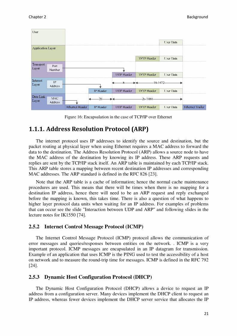
Chapter 2 Background
21
Figure 16: Encapsulation in the case of TCP/IP over Ethernet
1.1.1. Address Resolution Protocol (ARP)
The internet protocol uses IP addresses to identify the source and destination, but the packet routing at physical layer when using Ethernet requires a MAC address to forward the data to the destination. The Address Resolution Protocol (ARP) allows a source node to have the MAC address of the destination by knowing its IP address. These ARP requests and replies are sent by the TCP/IP stack itself. An ARP table is maintained by each TCP/IP stack. This ARP table stores a mapping between recent destination IP addresses and corresponding MAC addresses. The ARP standard is defined in the RFC 826 [23].
Note that the ARP table is a cache of information; hence the normal cache maintenance procedures are used. This means that there will be times when there is no mapping for a destination IP address, hence there will need to be an ARP request and reply exchanged before the mapping is known, this takes time. There is also a question of what happens to higher layer protocol data units when waiting for an IP address. For examples of problems that can occur see the slide "Interaction between UDP and ARP" and following slides in the lecture notes for IK1550 [74].
2.5.2 Internet Control Message Protocol (ICMP)
The Internet Control Message Protocol (ICMP) protocol allows the communication of error messages and queries/responses between entities on the network. . ICMP is a very important protocol. ICMP messages are encapsulated in an IP datagram for transmission. Example of an application that uses ICMP is the PING used to test the accessibility of a host on network and to measure the round-trip time for messages. ICMP is defined in the RFC 792 [24].
2.5.3 Dynamic Host Configuration Protocol (DHCP)
The Dynamic Host Configuration Protocol (DHCP) allows a device to request an IP address from a configuration server. Many devices implement the DHCP client to request an IP address, whereas fewer devices implement the DHCP server service that allocates the IP

Chapter 2 Background
22
addresses. If DHCP is going to be used by clients, there needs to be at least one DHCP server on the network (note that DHCP relays can be used to avoid the need to place a DHCP server on each sub network). The DHCP standard is defined in RFC 2131[25].
2.5.4 Transmission Control Protocol (TCP)
TCP provides a “connection oriented” service allowing reliable communication between two devices on an IP network. TCP relies on the IP service for the transmission of the TCP protocol data units.
TCP is based on several mechanisms to guarantee delivery. Initially the TCP source and destination perform a three-way handshake in order to set up a connection prior to sending data. They use a four-way handshake when tearing down the connection. In addition, all data must be acknowledged by the destination after it has been received. The TCP standard is defined in RFC 793 [26].
Most of the reliability sensitive internet applications such as web browsing, email, remote administration, and file transfer utilize TCP. Applications which do not require reliable sequential byte delivery use the User Datagram Protocol (UDP) which emphasizes reduced latency over reliability. Applications that need higher reliability with guaranteed delivery use the Stream Control Transmission protocol, standardized in RFC 4960 [77].
2.5.5 User Datagram Protocol (UDP)
Unlike TCP, UDP is a simple transport layer protocol that does not provide any flow control or delivery assurance mechanism. It does supports sequencing and reassembling of individual UDP datagrams. The sending node assumes that t a UDP datagram will reache the destination. An application that uses UDP takes responsibility of implementing its own mechanisms for the problems of reliability, detecting including message loss, and loss of connectivity. UDP is frequently used with delay sensitive data where low delay is more important than reliability.
The UDP protocol is very efficient because it is little more than a multiplexing mechanism on top of IP. Any additional semantics are the responsibility of the application. UDP does not require a connection and hence it can support broadcast and multicast transmission of datagram, i.e., where one node sends UDP datagrams to many (or all) destination nodes.
UDP protocol is widely used for media streaming (such as voice and video over IP) where an occasional lost packet does not matter. UDP standard is defined in the RFC 768 [27].
2.5.5.1 UDP frame format
A UDP data unit is called a “user datagram” and consists of two parts; a UDP header and a UDP payload. As Figure 17 shows, the header is divided into four 16-bit fields that specify the UDP port from which the message was sent, the UDP port to which the message is destined, the message length, and an optional UDP checksum.
Chapter 2 Background
23
Figure 17: UDP frame format The source port and the destination port fields contain 16-bit UDP port numbers. The
length field indicates the length of the UDP datagram in octets, including the UDP header and the user data. The data (payload) size can be up to 65,507 bytes in length. Use of the UDP checksum is optional though, it is the only way to guarantee the correctness of the data and that it has been delivered to the correct destination (as the checksum computation includes a pseudo header containing the source and destination IP addresses)
2.5.5.2 UDP Multiplexing, Demultiplexing, and Port numbers
All multiplexing and demultiplexing between UDP and higher layer applications occur through the port mechanism. UDP makes use of ports to distinguish among multiple applications utilizing the protocol. Both the destination port number and the source port number make it possible for UDP at the destination to deliver the datagram to the correct recipient applications and for the recipient applications to send a reply.
2.6 TCP/IP stack for CAN/Ethernet converter
As of today, there are many TCP/IP stack implementations available in the market. These are designed and implemented, and ported to most 8, 16, and 32 bit microcontrollers. We can categorize them into open-source TCP/IP stacks and commercial TCP/IP stacks. Open-source TCP/IP stacks include uIP [28], LwIP [29], and µC/TCP-IP [30]. NicheStack [31] is a commercial product. We chose an open source TCP/IP stack since this allows us to modify the code for our own purposes, if required, under the open-source license agreement. Even more importantly, we have the possibility to look at the code and understand how the stack works.
The µC/TCP-IP stack was developed for microcontrollers and embedded systems. The implantation is based on BSD code and therefore carries the BSD license*. The µC/TCP-IP is not popular because of its large memory requirement and limited support for its porting to ARM® microcontrollers.
The uIP (Micro IP) TCP/IP stack and the LwIP (Light Weight IP) TCP/IP stack have been developed by Adam Dunkels at the Swedish Institute of Computer Science (SICS)†. Dunkels, A. describes the main purpose of implementing the uIP TCP/IP stack as making it possible for small 8-bit microcontrollers to use TCP/IP protocol to communicate over the internet. Thanks to uIP TCP/IP, small devices with limited memory and processing capabilities can communicate over the internet. The typical implementation of uIP TCP/IP requires only a few kilobytes of ROM and, depending upon the application; RAM usage can be reduced to few hundred bytes. While it constitutes a complete TCP/IP stack implementation, the uIP TCP/IP stack features only the absolute minimal set of features. It
* http://en.wikipedia.org/wiki/BSD_licenses † http://www.sics.se/~adam/

Chapter 2 Background
24
can handle only one network interface and does not support UDP services; however, IP, ICMP, and TCP are available.
The LwIP TCP/IP stack implements IP, ICMP, UDP, and TCP. The LwIP TCP/IP stack supports multiple local network interfaces and has a flexible configuration and porting options making it suitable for a wide variety of devices. The LwIP TCP/IP stack is licensed under the BSD license.
As described earlier, in a CAN bus based system, a message sent by a node is received by each node attached to that CAN bus. The receiving node has to determine whether to make use of the message or discard it. The CAN/Ethernet converter we are designing uses UDP to emulate this CAN bus property. Using UDP the CAN/Ethernet converter can broadcast a message to all its peering nodes over an Ethernet. Therefore, among the open-source TCP/IP stacks, LwIP seemed to be the most suitable and appropriate for our purposes. It has already been ported to various microcontrollers and it supports multiple UDP sockets.
2.6.1 LwIP - A Lightweight TCP/IP stack
As mentioned earlier the LwIP stack was implemented to reduce memory usage and code size, making LwIP suitable for embedded systems with very limited memory. To achieve this, LwIP uses a custom API that does not require any copying of the data payload, when such data is transferred from one stack layer to another. This makes it possible for embedded systems to have internet connectivity if they have 10 kilobytes of RAM and around 40 kilobytes of ROM for the stack [29].
However, despite its limited requirement for memory, LwIP is a full TCP/IP implementation and supports the following protocols:
• IPv4 and IPv6 including packet forwarding over multiple network interfaces • ICMP for network maintenance and debugging • UDP supporting broadcast and multicast packet transmission and reception. • TCP with congestion control, RTT estimation, and fast recovery/fast retransmit. • DHCP • PPP • ARP • IGMP • SNMP
The LwIP TCP/IP stack does not include protocols from the application layer, such as HTTP or TFTP. It offers three application programming interfaces (APIs):
• Raw API: the native API used by the LwIP itself to interface with different protocols. • Sequential API: a sequential API with a higher level of abstraction than the raw API. • Socket API: a Berkeley socket-compatible API.
We decided to use raw API to integrate the CAN/Ethernet converter’s firmware with the LwIP TCP/IP stack. This API gives the highest performance and does not require the use of a real-time operating system, as the sequential API and the socket APIs do.
The LwIP TCP/IP stack consists of several modules where each TCP/IP protocol (IP, ICMP, UDP, and TCP) has been implemented as a separate module. A number of other support modules have also been implemented such as an operating system emulation layer, buffer and memory management subsystems, network interface functions, and functions for

Chapter 2 Background
25
computing the internet checksum. The use of modules enables us to only include the modules that we actually need for the CAN/Ethernet converter.
2.6.1.1 Packet buffers -pbufs
A packet buffer (pbuf) is a basic unit of memory in the LwIP buffer and memory management modules. Pbufs are similar to the mbufs* used in the BSD implementations. Network packets and socket buffers are stored in pbufs. A network packet may reside in one pbuf or it may span multiple pbufs arranged into a chain (i.e., a linked list) called a pbuf chain. Both dynamic memory as well as static memory can be allocated to a pbuf to hold the packet.
Pbufs are of three types with different purposes and usage: PBUF RAM, PBUF ROM, and PBUF POOL. Pbufs of type PBUF POOL are mainly used by network device drivers. Pbufs of type PBUF ROM are used when the data to be sent is located in the memory managed by the application itself.
Figure 18 represents the pbufs of type PBUF RAM. In this type, data stored in memory is managed by the pbuf subsystem itself. The PBUF RAM type is used when an application sends data that is dynamically generated, i.e. during runtime. The pbuf system allocates memory not only for the application data, but also for the headers that will be appended to the data.
A pbuf chain may consist of different types of pbufs. Incoming packets are stored in pbufs of type PBUF POOL and outgoing packets are stored in pbufs of the PBUF ROM or PBUF RAM types.
Room for Link Header
Next
Payload
Length
Total Length
Flags Ref
Room for IP Header
Room for TCP Header
Figure 18: A PBUF_RAM pbuf with data in memory managed by the pbuf subsystem (Source [29]).
Following functions are used for the handling of pbufs:
pbuf_alloc( ) Used to allocate pbufs of any of the three types described above.
* http://security.freebsd.org/advisories/FreeBSD-SA-10:07.mbuf.asc

Chapter 2 Background
26
pbuf_ref( ) Used to increase the reference count.
pbuf_free( ) Used to de-allocate a pbuf.
pbuf_realloc( ) Shrinks the pbuf so that it occupies just enough memory to cover the size of the data.
pbuf_header( ) Adjusts the payload pointer and the length fields for the header to be appended to the data in the pbuf.
pbuf_chain( ) Used to make the pbufs chain.
pbuf_dechain( ) Used to break the pbufs chain.
2.6.1.2 Memory management
The pbuf memory manager allocates contiguous memory locations for pbufs and deallocates previously allocated memory blocks. The memory manager uses a dedicated portion of memory in the system to ensure that the networking system does not use all of the available memory, and that the operation of application program is not disturbed if the networking system has used all of its allocated memory.
There are two types of memory management in LwIP: the heap memory (mem) and the static memory pools (memp). The packet buffer (pbuf) management manages both types; its own pbuf pool memory and the heap memory. The mem is a heap memory manager similar to the C malloc/free manager. A block of memory is allocated when mem makes a call to mem_malloc( ) and freed when it calls mem_free( ).
To allocate memory blocks of known size, the LwIP TCP/IP stack takes memory from a set of pools of fixed size blocks managed by memp. These fixed size memory blocks are used by LwIP for structures such as netconn, protocol control blocks, and packet buffers.
One can set the size of the heap, number of pbuf structures, and the number of Protocol Control Block (PCB) according to the application requirements.
2.6.1.3 IP Processing
Only the most basic functionalities of the IP have been implemented in the LwIP TCP/IP stack. It can send, receive, and forward packets, but cannot deal with fragmented IP packets or handle packets with IP options.
The function ip_output ( ) outputs a packet. It calls another function ip_route( ) to find the network interface to which the packet is to be forwarded. After the function ip_route( ) determines the appropriate network interface, the packet is forwarded via the outgoing network interface as an argument to ip_output_if( ). This function also takes the source and the destination addresses of the IP packet as an argument.
When a network device driver receives a packet from the network interface, it calls the function ip_input( ). This function compares the destination IP address with the IP address of the network interface to determine whether or not the packet is for this host. If the comparison is successful, then the protocol field is read to determine to which higher protocol the packet should be forwarded.
2.6.1.4 ICMP Processing
ICMP messages are encapsulated in an IP datagram for transmission. ICMP processing is quite simple because of its structure and function (see Figure 19). The LwIP function ip_input( ) receives packets and when the protocol field is 1 (i.e., ICMP) it forwards them to
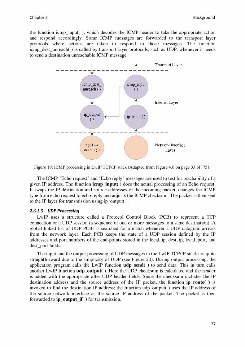
Chapter 2 Background
27
the function icmp_input( ), which decodes the ICMP header to take the appropriate action and respond accordingly. Some ICMP messages are forwarded to the transport layer protocols where actions are taken to respond to those messages. The function icmp_dest_unreach( ) is called by transport layer protocols, such as UDP, whenever it needs to send a destination unreachable ICMP message.
Figure 19: ICMP processing in LwIP TCP/IP stack (Adapted from Figure 4.6 on page 33 of [75]) The ICMP "Echo request" and "Echo reply" messages are used to test for reachability of a
given IP address. The function icmp_input( ) does the actual processing of an Echo request. It swaps the IP destination and source addresses of the incoming packet, changes the ICMP type from echo request to echo reply and adjusts the ICMP checksum. The packet is then sent to the IP layer for transmission using ip_output( ).
2.6.1.5 UDP Processing
LwIP uses a structure called a Protocol Control Block (PCB) to represent a TCP connection or a UDP session (a sequence of one or more messages to a same destination). A global linked list of UDP PCBs is searched for a match whenever a UDP datagram arrives from the network layer. Each PCB keeps the state of a UDP session defined by the IP addresses and port numbers of the end-points stored in the local_ip, dest_ip, local_port, and dest_port fields.
The input and the output processing of UDP messages in the LwIP TCP/IP stack are quite straightforward due to the simplicity of UDP (see Figure 20). During output processing, the application program calls the LwIP function udp_send( ) to send data. This in turn calls another LwIP function udp_output( ). Here the UDP checksum is calculated and the header is added with the appropriate after UDP header fields. Since the checksum includes the IP destination address and the source address of the IP packet, the function ip_route( ) is invoked to find the destination IP address; the function udp_output( ) uses the IP address of the source network interface as the source IP address of the packet. The packet is then forwarded to ip_output_if( ) for transmission.
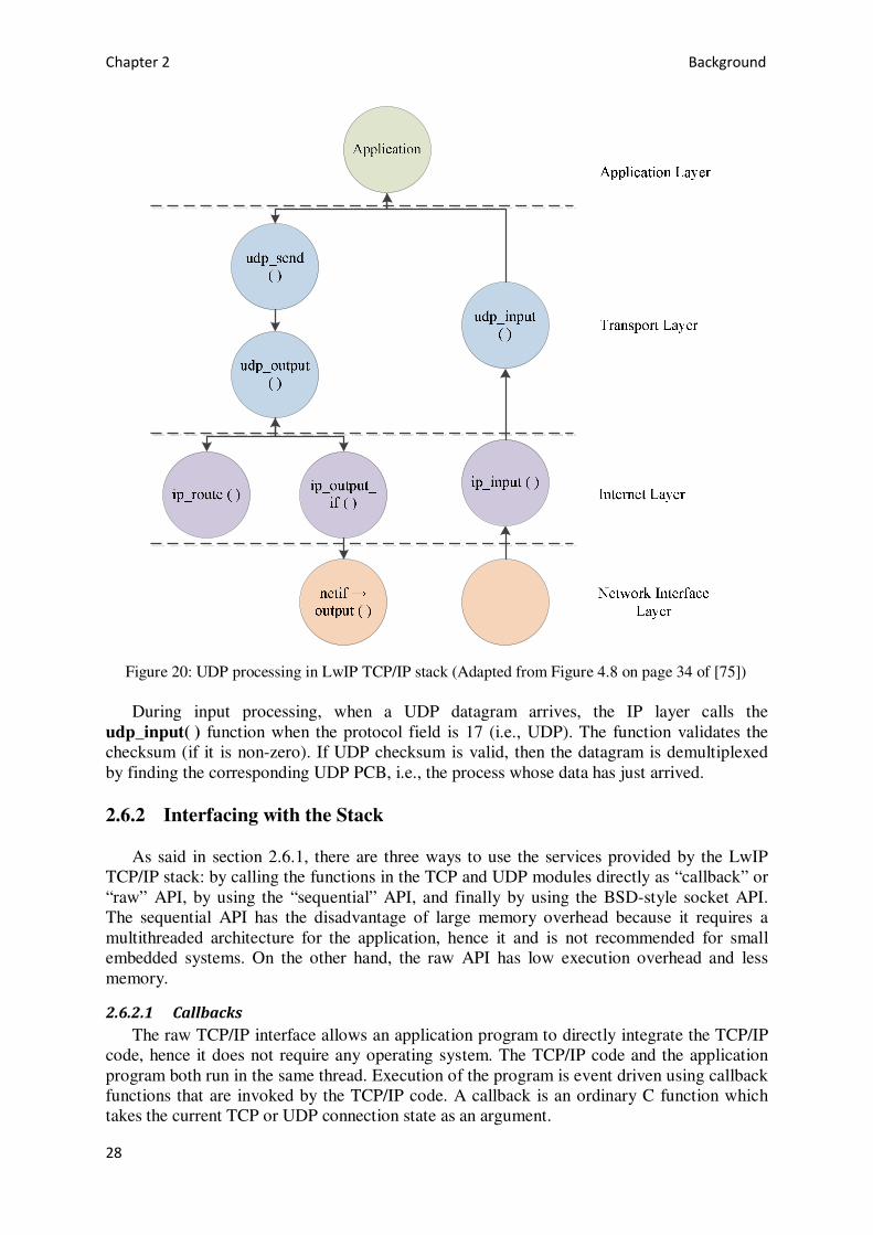
Chapter 2 Background
28
Figure 20: UDP processing in LwIP TCP/IP stack (Adapted from Figure 4.8 on page 34 of [75]) During input processing, when a UDP datagram arrives, the IP layer calls the
udp_input( ) function when the protocol field is 17 (i.e., UDP). The function validates the checksum (if it is non-zero). If UDP checksum is valid, then the datagram is demultiplexed by finding the corresponding UDP PCB, i.e., the process whose data has just arrived.
2.6.2 Interfacing with the Stack
As said in section 2.6.1, there are three ways to use the services provided by the LwIP TCP/IP stack: by calling the functions in the TCP and UDP modules directly as “callback” or “raw” API, by using the “sequential” API, and finally by using the BSD-style socket API. The sequential API has the disadvantage of large memory overhead because it requires a multithreaded architecture for the application, hence it and is not recommended for small embedded systems. On the other hand, the raw API has low execution overhead and less memory.
2.6.2.1 Callbacks
The raw TCP/IP interface allows an application program to directly integrate the TCP/IP code, hence it does not require any operating system. The TCP/IP code and the application program both run in the same thread. Execution of the program is event driven using callback functions that are invoked by the TCP/IP code. A callback is an ordinary C function which takes the current TCP or UDP connection state as an argument.

Chapter 2 Background
29
The application program specifies a callback function associated with a particular TCP or UDP connection. When a packet arrives for a TCP connection or UDP session, the corresponding callback function is called.
2.7 Ethernet Switch
As explained in section 2.4, today’s Ethernet devices are generally interconnected in a point-to-point or a star topology. In the star topology, the primary device which provides full duplex support to all network nodes is generally an Ethernet switch. The basic function of a switch is to receive frames on its input ports and forward them to their appropriate output port(s) based on the information in the frames. The term switch refers to a network bridge which, according to IEEE 802.1D [34], connects networks at the ISO/OSI layer 2, creates a separate collision domain for each port, and analyzes the incoming frames to provide enhanced MAC control.
2.7.1 Cut-Through vs. Store-and-Forward
Most modern switches provide several packet forwarding methods, specifically store-and-forward and cut-through (or adaptive-switching) [32].
Store-and- forward refers to a switching method in which frames are completely received and processed before being forwarded to the destination port. The processing includes calculating the CRC and checking the destination address. In addition, frames must be temporarily stored until network resources are available to forward the message.
In cut-through forwarding the switch begins to forward the incoming frame before it completely arrives. As soon as the switch knows the destination address, i.e. to which port the frame should be forwarded, the switch begins to forward the frame and does not wait for the complete arrival of the frame.
Although cut-through seems to be an efficient forwarding mechanism in terms of internal switching delay, it is not an alternative to store-and-forward operation. Cut-through operation is only possible if the destination port is available at the time the frame is received. If not, the switch must buffer the incoming frame and wait for the output port to become idle. Also, cut-through switch must be capable of store-and-forward operation when the input and output ports do not have similar data rates.
2.7.2 Data Flow Model
When a device connects to a switch port for the very first time, the switch stores the MAC address of the node and the port to which it is connected in an Address Lookup Table. The receive data path (which includes input buffer, address lookup table, VLAN table, and shared memory) performs all of the necessary qualification, classification, and lookup functions needed to determine to which output port an arriving frame should be forwarded. The transmit data path (which includes shared memory, output buffers, and priority scheduler) takes the forwarded frame, applies any prioritization and distribution policies, and sends the frame to the appropriate output(s). A switch fabric exists between the receive data path and the transmit data path. Its function is to move frames between the ports of the switch. Figure 21 shows a generic and simplified model of the flow of data in a shared memory based store-and-forward switch.

Chapter 2 Background
30
Figure 21: Ethernet switch data flow in Store and Forward switch (Sources: [32], [35], [36], and [40])
2.7.2.1 Input and Output FIFO
Each port has its own set of buffers for input (input FIFO) and output (output FIFO) to store an incoming frame before it is moved to the shared memory and the outgoing frame when it arrives from the shared memory and ready for the transmission.
2.7.2.2 Shared BUS
A shared bus architecture uses a common bus as the interconnect between input FIFO, output FIFO, lookup engine, and shared memory.
2.7.2.3 Address Lookup Engine
The lookup engine decides what to do with frames that have successfully passed through all of the prior buffering, classification, and VLAN filtering. The result of the lookup is a set of output ports to which a given frame should be forwarded.
Table lookup is performed against the filtering lists, Address Lookup Table, and IEEE 802.1Q [33] VLAN Table. These dynamically maintained lists contain the most recent

Chapter 2 Background
31
mapping of destination addresses and VLANs tags to the port(s) where the node(s) is/are connected.
2.7.2.4 Shared Memory
A shared memory is a common memory where incoming frames are stored temporarily before they are forwarded to the output FIFO. The shared memory plays a key role in the store-and-forward mechanism of the switch. Frames arriving through a receive data path are stored in the shared memory, and depending on the results from the Lookup Engine, frames in the shared memory are assigned and channeled to the transmit data path and later placed in the appropriate output queues of the ports.
2.7.2.5 Priority Scheduler
IEEE 802.1p queuing (discussed in the next section) allows the buffer scheduler to prioritize frames according to their types. Without priority scheduling, all frames wait in the same output queue if the receiving node is busy. In contrast, with priority scheduling, the scheduler places frames into output queues based on their priorities, which results in the lowest forwarding delay for frames with higher priorities.
2.7.3 Virtual LAN
Virtual LAN (VLAN) technology allows us to separate the logical connection from the physical connection of Ethernet nodes. In VLAN, nodes are logically grouped in a single broadcast domain irrespective of their physical location. One of many advantages of VLAN is the bandwidth reservation to enhance the performance. If a number of nodes are sharing time-critical data, they can be grouped together (logically) and separated (logically) from the other nodes that are sharing non time-critical data.
2.7.3.1 IEEE 802.1Q
The most common protocol used today in configuring VLANs is IEEE 802.1Q. The IEEE 802.1Q standard is part of the IEEE standard 802.1D. IEEE 802.1Q defines the architecture and services of a Virtual Bridged LAN and the protocols and algorithms involved in those services. It extends the 802.1D functionality in a number of areas such as mostly filtering database, frame tagging, priority operation, switch management, etc. Since we are mostly concerned with priority based frame forwarding, we will look briefly into the 802.1Q VLAN tag format.
2.7.3.2 IEEE 802.1Q VLAN Tag
An 802.1Q VLAN tag comprises three elements: VLAN Protocol Identifier (VPID), Tag Control Information (TCI), and Embedded Routing Information Field (E-RIF)
VLAN Protocol Identifier (VPID) It tells the devices that the frame is a VLAN tagged frame; thereby to differentiate tagged frames from untagged frames.
Tag Control Information (TCI)
Apart from other fields, it contains a 3-bit priority filed that indicates the user priority of the frame. It is for the benefit of IEEE 802.1p (priority-aware) switches. By adding this information in the frame, burden over the switch has been avoided where it had to determine frame priority by parsing the frame

Chapter 2 Background
32
and applying a set of priority rules. Embedded Routing Information
Field (E-RIF)
An optional field that carries source routing information for networks not supporting the local source routing.
2.7.3.3 IEEE 802.1p
IEEE standard 802.1p [34] is a part of the IEEE standard 802.1D. The 802.1p standard covers the traffic class expediting and dynamic multicast filtering part of MAC bridges. It describes mechanisms to prioritize traffic in which lower priority frames are not sent in the presence of higher priority frames for the same destination port.
To use IEEE 802.1p, the IEEE 802.1Q Ethernet format must be adopted. IEEE 802.1p sets a 3-bit value in the MAC header to indicate prioritization. This 3-bit value provides priority levels ranging from 0 to 7, with level 7 representing the highest priority. This permits packets to cluster and form different traffic classes. Thus, when network congestion occurs, those packets that have higher priorities will receive special treatment while low priority packets will be kept buffered. When a frame is not a VLAN tagged frame, an IEEE 802.1Q compliant switch associates the untagged received frame with a VLAN identifier based on the port on which the frame arrived, i.e., priority is assigned as per port.
Because of its support for priority specification, IEEE 802.1p is important for providing Class of Service (CoS) for better reliability and quality. Details of this are described below.
2.7.3.4 Quality of Service
Quality of Service (QOS) is a level of guarantee given to a critical frame that it will make its way to the destination within some bounded time. QoS establishes some sort of an end-to-end path in the network such that it makes every device on that path to guarantee a certain level of service to a specific frame. If a device that will be part of that path cannot guarantee the required level of service, then this device can reject the request t hat it be a part of that path or it can offer a guarantee for a lower level of service.
2.7.3.5 Class of Service
A Class of Service (CoS), in contrast to QoS, neither establishes specific path in the network, nor makes any explicit guarantees. CoS simply allows the sender to prioritize a frame according to its importance. The highest priority class gets the best available service at every device in the network, but none of these devices guarantee any specified minimum level of service.
CoS is easier to implement in the sense that a switch does not have to remember the state information of every flow. Priorities are assigned independently to frame. The switch provides the best available service to a higher-priority frame by putting it in an appropriate higher CoS queue. Channel bandwidth does not need to be reserved and no request is required from the sender to establish an end-to-end path as in QoS.
2.8 Latency in a switched Ethernet network
Latency or network delay in communication network is generally described as the amount of time it takes for a signal or a data packet to traverse the network, starting from the node that initiated the transmission and ending at the destination node.
Latency from the source to the destination is often called end-to-end latency or one-way latency. Whereas if the destination node has to reply on the received message then the
Chapter 2 Background
33
“round-trip latency” is the time it takes from the initial message being sent until the reply message arrives at the source.
2.8.1 Sources of Latency
Switched Ethernet networks have several sources of latency which impede the message flow when it traverses various components of the network such as wires, cables, and switches [35] [36].
In this thesis we are interested in the following sources of latency; store and forward latency (store-and-forward switch), cut-through latency (cut-through switch), switch fabric processing latency or switch internal routing delay, wireline or propagation delay, queuing latency, blocking latency, and interference latency. All of these latencies are known a priori
except queuing, blocking, and interference latencies; however, these delays can also be calculated provided one knows the nature of all sources of traffic on the network and the behavior of the switch.
Here we do not take into consideration the internal delay of the source node or the receiving node since this delay depends on the network interface card, operating system running the application, and the TCP/IP stack.
Below we explain in detail each of the sources of latency described above in the context of a switched Ethernet network. Based upon these delays we can calculate the expected worst case latency.
2.8.1.1 Ethernet switch latency
As said in section 2.7.1, forwarding of frames in an Ethernet switch is done in two ways: store-and-forward and cut-through. In cut-through, the switch delays the flow of frame only long enough to decode the destination’s MAC address and other header fields (e.g., VLAN tag and 802.1p priority field) in order to make a forwarding decision. Switching latency is thus reduced as the processing delay is restricted to processing the header instead of the entire frame. Whereas in store-and-forwarding the switch stores the complete frame before it makes forwarding decision thereby increasing the switching latency.
2.8.1.1.1 Cut-Through latency (���)
A cut-through switch begins forwarding the frame to the destination as soon as the switch finds the appropriate output port (if idle) to which this destination address is mapped. This means that a cut-through switch can overlap the processing (serialization) of the outgoing frame with the processing (serialization) of the incoming frame. The switch latency can be measured as the difference in time when the first bit of the frame enters the switch and the first bit leaves the switch (FIFO). Therefore, the corresponding network latency in a single hop cut-through (CT) switched network is
��� = �� �� ��� ������� + ������ ���������� � (eq. 1)
Where,
�� �� ��� ������� =�������� ��
� �!"���� ���+ �����#���� �$(��&)
The network latency for the cut-through switch is lower for two reasons: (1) only one instance of serialization delay is encountered, which can be a significant factor for larger frame sizes, and (2) the switch latency is lower because of the inherent simplicity of cut-through switching. No CRC verification is done in these switches.

Chapter 2 Background
34
2.8.1.1.2 Store-and-Forward latency (�())
A store-and-forward switch waits for the whole frame (serialization) before it begins its processing. Once a frame is completely received, the integrity of the frame is verified by computing the CRC field of the received frame, then the frame can be comparing it with the CRC and forwarded immediately to the output port. The switch latency for a frame is measured as the delay between when the last bit enters the switch and the first bit leaves (LIFO) the switch. Also, the serialization delay occurs twice as the switch has to serialize the frame once more to deliver it to its destination. Therefore, the network latency for a one hop store-and-forward (SF) switched network is:
�� = * × �� �� ��� ������� + ������ ���������� � (eq. 2)
Even though store-and-forward switches have the disadvantage of an extra serialization delay, in certain cases this delay is quite useful. For example if the ingress port and egress port have different link rates, then the incoming frame must be transmitted only when it is completely received and buffered. Another advantage would be in higher load at egress port when there are more than one incoming flows, in this case some of the frames have to be buffered. Thus, in some cases store-and-forward switching have an obvious advantage.
2.8.1.2 Switch Fabric Latency (�,)
The switch fabric includes the internal architecture of the switch built around logic elements such as Field Programmable Gate Array (FPGA), Application Specific Integrated Circuit (ASIC), FIFOs, and shared memory that together implement the store-and-forward or cut-through flow control, address lookup engine, priority scheduler, etc. The switch fabric introduces delay in executing the logic elements that implements these functions. Switch fabric latency varies from manufacture to manufacture.
2.8.1.3 Wireline Latency (�,�)
The wireline latency or propagation delay is the time a signal takes to physically traverse the path (wires or fiber optics). The delay is directly proportional to the distance between sender and receiver and the speed of propagation in the media. It is assumed that the signal passing through wires or fibers travels at two thirds the speed of light [76]. When an Ethernet link spans a long distance, the resulting delay becomes significant. For example, the one way latency for a 1km link is:
�,� =-...�
*/× / × -.0�/�
�,� = 23�
For shorter distances in local area networks, this delay is very small in comparison with the other sources of latency. For high performance time critical networks with long links, the wireline latency affects the overall end-to-end latency, and therefore cannot be ignored.
2.8.1.4 Queuing Latency (�4)
When many ingress ports are active simultaneously, such that there is more than one flow entering the switch with the same destination address, i.e. the same egress port, then the switch queues the incoming frames in a shared memory. The rate at which the queue builds up depends on the data rate at which the ingress ports receive their frames and the link rate of

Chapter 2 Background
35
the egress port. Queuing introduces a non-deterministic factor to latency since it can often be very difficult to predict exact traffic patterns on a network.
Research has been done to calculate the maximum queue size and the queuing delay in Ethernet switches. First Cruz [37] then Boudec and Thiran [38] proposed a theoretical model to calculate network behavior. Calculating the worst case latency for any Ethernet frame with precision requires detailed knowledge about all sources of traffic on the network, maximum frame size in any flow, CoS priority of frames, and bandwidth utilization.
2.8.1.5 Blocking latency (�5)
The QoS technique proposed in IEEE P802.1p appends a 3-bit priority field to the Ethernet frame header (IEEE 802.1Q) to classify the priority of the stream in order to improve the real-time behavior of switched Ethernet. Also manageable switches have a port priority feature where one can set the port priority according to the significance of the incoming flow on this port. Although both techniques help deal with queuing latency, frames with the highest priority level still are enqueued relative to one another [39].
Additionally, if the transmission of a lower priority frame has already started before a higher priority frame is enqueued, then the lower priority frame transmission must finish first before the switch begins transmitting the higher priority frame. Lext, Bröhne, and Andersson describe this behavior of the switch as blocking [40]. This is due to the non-preemptive nature of the switch, i.e., it does not suspend the transmission of a lower priority frame when there is a higher priority frame that arrives during the transmission of the lower priority frame. The higher priority frame has to wait for at least one serialization time of the lower priority frame before it can leave the switch. The worst case will occur when all ports are active and all incoming frames have the same destination address, in this case if all of the frames have the same priority and all are destined to the same outgoing port, then some port will have to wait for all but one of the other frames to be transmitted before it gets its turn, one has to wait for all but two frames to be transmitted, another for all but three frames, etc.
2.8.1.6 Interference latency (��)
Lext, Bröhne, and Andersson. also describe another term called interference [40] that occurs when a lower priority frame has to wait for a higher priority frame when both arrive at their respective ports simultaneously and are destined to a common node.
2.8.2 Total Worst-Case Latency Calculation (������)
The latency sources described above are duplicated for every switch that an Ethernet frame must traverse on its journey from source to destination. The worst-case latency in multi-hops switched (store-and-forward) network is comprises of the above said latencies and in general,
����6� = ∑ [�� + �, + �,� + �4 + �5 + ��]� ����� � (eq. 3)
2.8.3 TCN Analyzer and Latency in Ethernet network
The analysis engine of the TCN Analyzer (discussed in the next section) uses the above equations to compute an upper bound on the worst case latency [40]. It also uses additional equations to find individual sources of latency, particularly for calculating delays due to interference (��) and blocking (�5)
Chapter 2 Background
36
In addition to blocking, an occasional priority-inversion adds additional delay to the forwarding time of the higher priority frame. Priority-inversion occurs when the Ethernet switch forwards a lower priority frame on a link although a higher priority frame requests that same link. This happens occasionally when a switch forwards a lower priority frame waiting in the queue in between the transmission of a high priority flow consisting of a burst of frames.
2.9 TCN Analyzer
TCN Analyzer is a tool to design Ethernet networks for time-critical applications [41]. The network designer can use TCN Analyzer to construct a virtual Ethernet network based on virtual switches and hosts, virtual paths, and flows with any standard payload sizes. The designer can configure the virtual switches with different port priorities and link speeds. TCN Analyzer computes an upper bound on the delay which we call the “forwarding time” for an Ethernet frame of all flows across the switch, i.e., no frame in the real network would be delayed for longer than what TCN Analyzer predicts.
2.9.1 Computational Engine
The computation is carried out by an analysis engine running within the TCN Analyzer. Based on the network parameters that the designer inputs to the tool when modeling a virtual Ethernet network, the engine utilizes these parameters in a set of formulae and equations to compute the upper bounds on frame latency, response time, and maximum frame buffer space required in each switch.
These formulae and equations correspond to a sum of delays and latencies that an Ethernet frame suffers while traversing the network from source to destination node. The formulae correlate the sources of latency and delays as described in the previous section with each other and with the parameters given to the engine such as payload size, port priorities, and link speeds. The engine integrates a timing model of every component used in the network and also considers every other entity that competes for shared resources in the network. Therefore we have an exact timing (bound) analysis of the flows in the network.
2.9.2 Switch modeling
An Ethernet switch is modeled to include all those factors and aspects of a switch which as described in the previous section that cause the delays. These aspects include:
• Link speeds of each enabled switch port (ingress and egress), • The internal packet scheduling algorithm specific to switch manufacture, • Amount of memory (input/output FIFOs and shared) available to incoming and outgoing frames,
• Non-ideal behavior (e.g. priority inversion due to defective switch behavior), • Port or flow priority settings.
2.9.3 Transmission medium modeling
Here the wireline delay is modeled according to the transmission medium, e.g., CAT5 cables or optical fibers. Two parameters are used to model a link: the cable length and the propagation velocity of an electromagnetic wave as it travels along the fiber- or cable medium.
Chapter 2 Background
37
2.9.4 Frame modeling
Here the Ethernet traffic called a “flow” is modeled. TCN Analyzer assumes that each flow in the network is a sequence of frames such that each frame in a flow has the same source and destination address and always traverses a single path. The frame in a flow is modeled by TCN Analyzer using the following parameters (as input by the network designer):
• Frame payload size, • Deadline of the frame from source to destination (i.e., the maximum time a frame can take to
traverse the network), • Frequency or the period of transmission of frames from the source node (i.e., the minimum
time interval between which the source generates frames), and • Protocol (TCP or UDP). (Currently TCN Analyzer only supports UDP frame modeling).
2.9.5 Flow modeling
Before the analysis can start, the analysis engine of the TCN Analyzer needs to know from the network designer the path taken by each flow through the network. In a standard Ethernet, the Rapid Spanning Tree Protocol (RSTP) selects paths of the flow so that a cyclic-free tree is constructed [34]. The RSTP tree defines the route taken by each flow through the network.
In TCN Analyzer once the hosts, switches, and frames are initialized, then the designer has to define the flow across the switch in order complete the construction of the virtual network. Here source node, destination node, type of the frame, number of frames in a burst, and priority of each flow are defined. Figure 22 shows how the graphical user interface of TCN Analyzer when a complete network along with every component has been defined and initialized for real-time analysis.

Chapter 2 Background
38
Figure 22: Graphical user interface of TCN Analyzer (Courtesy of Time Critical Networks AB)
2.9.6 Performing the analysis
After the analysis engine has performed its computations, TCN Analyzer displays the upper bounds of the forwarding time of each frame of every flow. Furthermore, the memory in the switch that will be required for this topology of network is also presented. This later information tells if the switch will drop packets due to memory overflow. One can verify if all constraints are met, i.e., all the deadlines are met and no buffer memory overflow (which could lead to a packet drop) occurs. If any of the constraints are violated, then the designer can experiment with different parameters such as priority settings, link speeds, network topology, etc. until the forwarding time meets the desired deadline and all the real-time requirements have been met.
2.10 Prior work
Prior work on this topic has primarily focused on the implementation of special protocols or modifications of existing protocols on different layers of TCP/IP stack. Network topologies such as ring, star, master/slave etc. have been considered to make the time delay for message delivery deterministic. The other category of research includes the analysis of the real-time performance of Ethernet networks to calculate and estimate the various types of delays that occur in an Ethernet switch in order to compute the worst case latency. Computation of these delays was explained in detail in section 2.8. Another relevant work is the comparison of the worst case latency or forwarding time obtained from the modeling of an Ethernet network in a simulator with a similar implementation in the real world.

Chapter 2 Background
39
There are two classifications of the real time implementation of Ethernet: [42] and [43]. Decotignie [42] classifies real-time implementations according to the level of compatibility with standard Ethernet namely incompatible, non-interoperable, interoperable homogeneous, and interoperable heterogeneous.
Incompatible implementations modify the MAC protocol and in that way require a change in the Ethernet hardware (or firmware) as well. An Ethernet node compliant with Non-interoperable protocol cannot work with other network nodes that do not implement the protocol. Interoperable homogeneous implementations allow its Ethernet nodes to work together with standard Ethernet nodes. However, most interoperable homogeneous implementations assume all devices use the same modifications. While the interoperable heterogeneous compatible Ethernet nodes can work together with standard Ethernet nodes that do not adapt the same modifications.
Felser [43] classifies real-time implementations according to the layer in the TCP/IP stack where modifications are introduced. This classification is illustrated in Figure 23. When TCP/UDP/IP protocols remain unchanged and all the real-time modifications are done in the top layer it is called “On top of TCP/IP.” On the other hand when the TCP/UDP/IP protocols are bypassed and the Ethernet MAC layer is accessed directly these modifications are called “On top of Ethernet”. Lastly, when the MAC layer itself is modified to make Ethernet more real-time these modifications are called “Modified Ethernet”. The following subsections describe each of these alternatives.
2.10.1 Realization on top of TCP/IP protocols
The most popular real-time Ethernet solutions on top of TCP/IP include the MODBUS TCP/IP [44] standard with its real-time extension of the Real-Time Publisher Subscriber (RTPS) protocol, the EtherNet/IP protocol [45] that provides real-time communication by assigning the IEEE 802.1Q VLAN tag priority to the time critical messages, and the P-NET on IP specification [46] designed to enable the use of P-NET real-time communication wrapped into UDP/IP packages.
Figure 23: Possible real-time Ethernet realizations

Chapter 2 Background
40
2.10.2 Realization on top of Ethernet
The implementations on top of Ethernet are typically those that use time scheduling mechanism such as slicing and slotting inside the MAC layer. Examples are Ethernet Powerlink (EPL) [47], Time-critical Control Network (TCnet) [48], Ethernet for Plant Automation (EPA) [49], and PROFINET [50] [51]. These real-time Ethernet realizations do not modify the Ethernet hardware. Instead, they specify a special type value (Ethertype) in the Ethernet frame. These protocols use their own TCP/IP stack in conjunction with their own protocol type in addition to using the standard IP protocol stack.
Yiming and Eisaka present another protocol on top of Ethernet for hard real-time industrial application based on the QoS feature [52]. The protocol supports real-time traffic as well as non-real time traffic and doses not modify the hardware. Yiming and Eisaka claim that by using the proposed protocol latency can be reduced to 32% comparing with the UDP/IP protocol and more than 50% comparing with the TCP/IP protocol on the same Ethernet node.
2.10.3 Realization with modified Ethernet
The implementations that use modified Ethernet intend to support the existing topologies used in factory automation (such as bus and ring) with switched Ethernet using star topology. An argument for not using a star topology with switched Ethernet was the cabling cost. To allow daisy-chained bus or ring topology and to avoid the star topology, while achieving the real-time performance at the same time, the switching functionality is integrated inside the network devices. This modification is mandatory for all devices attached to the real-time network, but they allow non real-time traffic to be transmitted without modifications.
A few realizations with modified Ethernet are SERCOS (SErial Real-time COmmunication System Interface) [53], EtherCAT [54], and PROFINET Isochronous Real Time (IRT) [55] [56].
The EtherCAT protocol uses a master/slave technique together with specialized switches and an open-ring topology to achieve real-time performance. The master initiates every transaction and thus has complete control of the network. Seno and Zunino have simulated the performance of EtherCAT networks [57]. Theoretical analysis and numerical simulations have been performed with a focus on the cycle time of an EtherCAT network as the performance indicator.
PROFINET IRT, a new PROFINET real-time profile, employs a time slotting scheme in the communication cycle by dividing it into a deterministic time-triggered phase and an open phase. The cyclic real-time messages are transmitted using the deterministic channel, while non-real time TCP/IP messages are transmitted through the open channel. Hoang et al. propose another approach by using the Earliest Deadline First scheduling policy and online admission control in an Ethernet switch [58].
Loeser and Haertig propose a different technique and use a traffic shaper at each node to regulate the burst and the load over the network in a way that prevents memory overflows [59].
Chapter 2 Background
41
2.10.4 Realization with cots switches
This approach uses standard switched Ethernet infrastructures, i.e., COTS switches, network interface cards (NIC), and IP stacks. The Flexible Time-Triggered Switch Ethernet (FTT-SE) protocol [60], an adaptation of FTT Ethernet protocol in micro-segmented networks, is build around COTS switches with one switch port connected to one station. Since it is a master/slave protocol it introduces additional overheads.
2.10.5 Numerical simulation and practical verification
Gutiérrez, Palencia, and Harbour [61] analyzed the response-time of the Avionics Full Duplex Switched Ethernet (AFDX) network including the scheduling of the virtual links and contention in the end-systems and in the switches. Using this response-time they obtained worst-case latencies and output jitter for AFDX networks. A real-time model is defined for a communication network based on AFDX which includes modeling of the queuing effects in the nodes and in the AFDX switches, and the end-to-end response times. From such model, they have developed a response-time analysis method for AFDX networks.


3 Method This chapter explains in detail the methodology we followed to carry out the research. It
explains the execution part of the three methodological segments of the project. Analysis on the results and outcomes of methods explained in this part are discussed in chapter 4.
3.1 Introduction
As mentioned in the section 1.3 the methodology we decided to follow had three phases. These three phases were: theoretical evaluation (network modeling using TCN Analyzer), verification of the results of theoretical phase and validation of the proposed CAN/Ethernet network on the test rigs of CPAC Systems.
3.2 Theoretical evaluation / simulation
We modeled various Ethernet networks built around a single managed switch, one destination (sink), and one or more sources. We had used one switch in every configuration as the CPAC Systems initial requirements could be satisfied with only one switch. We tried to create situations where a UDP frame carrying a CAN message could undergo the worst case delay or maximum forwarding time in traversing the network from source to switch and eventually to destination.
However, in doing so, we needed to prevent the loss of packets due to the limited memory of switch by avoiding overloading the switch. That is, we maintained in every measurement the condition that the sum of ingress data rate should not exceed the sum of egress data rate. Since the egress data rate was 100 Mbps on a single sink, the total ingress data rate in each measurement never exceeded 100 Mbps. We imposed a hypothetical limit which was relevant to our proposed CAN/Ethernet network.
3.2.1 Westermo RedFox switch
The switch model that was used in TCN Analyzer for the construction of network is a store-and-forward type of switch from Westermo, specifically their RedFox RFI-10 industrial Ethernet switch [62]. TCN Analyzer has modeled this switch according to the hypothesis of the delays that occur inside a switch (as explained in chapter 2) according to its internal architecture, specifications, features, etc. We also used the RedFox switch in the practical evaluation, verification, and in the final phase of validation on CPAC Systems test rigs. The switch specifications are shown in Table 3.

Chapter 3 Method
44
Table 3: Westermo RedFox RFI-10specifications [62]
Electrical specification IEEE std 802.3. 2005 Edition
Data rate 10 / 100 Mbps, manual / auto
Duplex Half / Full, manual / auto
Transmission range Up to 150 m with cat5e cable
Connection RJ-45 auto MDI/MDI-X
Number of ports 10 (2: Single-Pair High-speed Digital Subscriber
Line (SHDSL) + 8: Ethernet)
Layer-2 Switching IEEE 802.1Q Static VLAN and VLAN Tagging
Layer-2 QoS IEEE 802.1p Class of Service
3.2.2 Network model
We discussed the modeling of an Ethernet network using TCN Analyzer in section 2.9. In this section we discuss the parameters of the network components as configured in TCN Analyzer. We modeled the network with different numbers of flows and with different amounts of data ranging from the minimum to maximum allowable payload size in a single UDP frame without fragmentation (since LwIP TCP/IP does not support fragmentation)
3.2.2.1 One flow
We began with one flow, i.e. there was only one source which we called CEC1 (CAN/Ethernet Converter 1) that sent UDP packets to one sink which we called H2. We picked the RedFox switch as the Ethernet switch and linked CEC1 to port 1 of the RedFox switch and H2 to port 2. We set the ingress and egress link speed of each port to 100 Mbps. In the frame template editor we created a frame named UDPFrameTemplate, chose UDP as the protocol and set the next release time to 1000 µs (i.e., the frame would be emitted every 1ms). In the flow editor we created a flow named “Flow0” and picked CEC1 as the Source Node and H2 as the Destination Node. We did not choose any burst since we decided to model periodic flow with a uniform data rate and therefore set the multiframe parameter to 1.
We ran TCN engine to compute the upper bound on the forwarding time, i.e., latency, of the Ethernet frame in Flow0. We calculated four estimates with UDP payload lengths of 22 bytes, 472 bytes, 972 bytes, and 1472 bytes. Note that a CAN message can completely reside in a UDP payload of 22 bytes size. Measurements with the three other UDP payload sizes were carried out to see how it would affect the forwarding time of a critical flow carrying a CAN message when we have other UDP flows carrying large frames such as video, voice, GPS etc.
We followed the same procedure with two number of flows, three, and up to seven flows. In every estimate, we set the priority of CEC1 to “0”, the lowest priority, to cause TCN engine compute the worst case forwarding time for critical frames of the flow CEC1. Figure 24 shows the parameters set in TCN Analyzer for a single flow configuration.

Chapter 3 Method
45
Figure 24: One flow modeling in TCN Analyzer
3.2.2.2 Four flows
We increased the number of flows from one to four into the Ethernet switch in order to see how this additional traffic would affect the forwarding time of the UDP frame generated by CEC1, i.e., the critical flow carrying the CAN message. The other flows were non-critical flows acting as background traffic to create delays for the critical flow CEC1 in the switch.
There were four sources CEC1 to CEC4 that send UDP packets to a common sink H2. We chose the same RedFox switch as the Ethernet switch and linked CEC1, CEC2, CEC3, CEC4, and H2 to port 1, port 3, port 4, port 5, and port 2 respectively. We set the ingress and egress link speeds to 100 Mbps. In the frame template editor we created a frame, picked UDP as the protocol, and next release time to 35 µs (for the case when the payload size was 22 bytes). The next release time value was chosen such that the sum of the ingress data rate would be less than the egress data rate to avoid any packet drops inside the switch. In the flow editor we created flow “Flow0” and picked CEC1 as its Source Node and H2 as its Destination Node. Similarly we created flow “Flow1” and picked CEC 2 as its Source Node and H2 as its Destination Node and followed the same procedure for the remaining two flows “Flo 2” and “Flow3”.
After the network had been parameterized, we used TCN engine to compute the upper bound on the forwarding time or latency of the frame in Flow0 which carried our critical CAN message. We performed four estimations with UDP payload sizes of 22 bytes, 472 bytes, 972 bytes, and 1472 bytes and next release time of 35 µs, 234 µs, 465 µs, and 691 µs respectively. In every measurement, we set the priority of CEC1 to “0”, the lowest, and
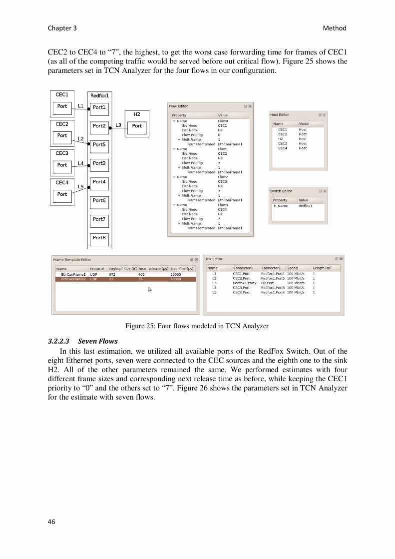
Chapter 3 Method
46
CEC2 to CEC4 to “7”, the highest, to get the worst case forwarding time for frames of CEC1 (as all of the competing traffic would be served before out critical flow). Figure 25 shows the parameters set in TCN Analyzer for the four flows in our configuration.
Figure 25: Four flows modeled in TCN Analyzer
3.2.2.3 Seven Flows
In this last estimation, we utilized all available ports of the RedFox Switch. Out of the eight Ethernet ports, seven were connected to the CEC sources and the eighth one to the sink H2. All of the other parameters remained the same. We performed estimates with four different frame sizes and corresponding next release time as before, while keeping the CEC1 priority to “0” and the others set to “7”. Figure 26 shows the parameters set in TCN Analyzer for the estimate with seven flows.

Chapter 3 Method
47
Figure 26: Seven flows modeling in TCN Analyzer
3.3 Practical evaluation / verification
In this phase we evaluated and verified practically the estimations made by TCN Analyzer for the upper bound on the frame forwarding time for various Ethernet network configurations. To perform evaluation and verification of the results obtained from TCN Analyzer for the worst case latency it was obvious to use the same network topology, same switch, same number of sources and sink, and Ethernet medium etc. Therefore to reach that upper bound limit under comparable constraints which were imposed on TCN Analyzer, we had used a similar network, that is, we used the same RedFox switch, one up to seven sources that sent UDP frames to one destination only and kept the same data rate and payload sizes in each setup.
3.3.1 Achieving TCN Analyzer upper bound
To achieve TCN Analyzer predicted upper bound of the worst case latency, we have to characterize the network in a way to reach that limit. In section 2.8 we discussed in detail the latency in a switched Ethernet and the assumptions that TCN Analyzer makes in calculating the forwarding time. To reach the worst case limit, we have to increase the probability of satisfying those assumptions.

Chapter 3 Method
48
In section 2.8 we discussed the total worst case latency which consists of store-and-forward latency, switch fabric latency, wireline latency, queuing latency, blocking latency, and interference latency. Except for queuing, blocking, and interference other sources of latencies are known a priori and do not need any special attention in the practical evaluation. However, in order for the Ethernet frame to suffer queuing, blocking, and interference latencies, special attention must be paid in order to create an identical configuration of the required network components. These three types of latencies occur when two or more frames arrive at the switch ports simultaneously, although the frames are generated from different sources, they all are being forwarded towards a common destination. In this situation some frames must be enqueued in the switch’s memory while waiting for the egress interface to be idle. Moreover simultaneous arrivals will result in blocking of higher priority frames and interference as well.
Therefore to achieve the simultaneous arrival of frames at the switch ports, we need to maximize the probability of “simultaneous frame arrival”. Figure 27 depicts the simultaneous arrival of all of these frames and the delay suffered when these frame arrive at their corresponding switch ports simultaneously. There are two flows with slightly different data rate and hence differing periods. The red flow has a higher data rate than the green flow.

Chapter 3 Method
49
12
34
5
12
34
56
67
89
10
78
Hea
dT
ail
Tim
e
Tim
e
Hea
dT
ail
Peri
od
Red
<P
eri
od
Gre
en
Rat
e R
ed>
Rate
Gre
en
Per
fect
sim
ult
aneo
us
arri
val
Figure 27: Perfect simultaneous arrival of Ethernet frames

Chapter 3 Method
50
In order to maximize the probability of frames arriving simultaneously, we chose the data rate from the prime numbers. A prime number can be divided, without a remainder, only by itself and by 1, and it does not have any multiples or divisors. Therefore the two UDP flows do not alias to each other and they do not have a common phase difference. If one imagines a time slot or window and takes one flow as reference, the other flow would appear to shift in time due to varying phase difference.
To increase the probability of simultaneous arrivals, we must choose the interarrival frequency of the frames such that the sum of ingress data rate is less than the 100 Mbps egress link rate. This is a condition we maintained in every configuration and in every flow setup while modeling the network in TCN Analyzer.
Initially, the green frames arrive earlier than the red frames in the shown time slots in Figure 27. When they arrive at (nearly) the same time, the red frame partially overlaps the green frame. The red frame has to wait an amount of time enqueued in the switch queue which is equal to the length of its frame overlap with the green frame. When a red frame and a green frame arrive at their respective ports simultaneously and thus their arrival times overlap, the red frame has to wait in the switch queue for one complete green frame time. It should be noted that the green frames did not suffer any delay due to near simultaneous arrival since it always arrived a head of the red frame.
Following after the perfect simultaneous arrival, the rd frames start to appear earlier than the green frames in time slots and therefore the green frames will suffer delays due to this near simultaneous arrival. As shown in Figure 27, similar kinds of delays are faced by the green frames after the simultaneous arrival of both red and green frames.
3.3.2 Preliminary proposal limitations
In the initial proposal for this master thesis project, it was said that during the practical evaluation phase, the source and destination nodes would be CAN/Ethernet converters. That is, there would be a CAN/Ethernet converter that would receive a CAN message generated by a CAN node (CAN message generator), encapsulate it into UDP payload, and finally send the UDP frame to an Ethernet switch. At the destination, there would be another CAN/Ethernet converter that would receive that UDP frame, extract the CAN message from the UDP payload, and finally send the CAN message to the CAN node (CAN message receiver).
However, during the evaluation phase we came across a situation which we had not taken into consideration at the beginning. The situation arose from the fact that today the maximum data rate standardized in a CAN bus is 1 Mbps. This implies that the maximum data rate at which a CAN/Ethernet converter can receive Ethernet frames would be 1 Mbps. Whereas the Ethernet links from source to switch and from switch to sink/destination used in the project operated at 100 Mbps. Therefore when using a CAN/Ethernet converter as a sink or destination the CAN/Ethernet converter could convert a 64 bytes Ethernet frame that arrived at 100 Mbps (every 6.08 µs) and after conversion send 20 bytes CAN messages to CAN nodes. However, unless the converter does buffering it would try to emit CAN messages at 26 Mbps (every 6.08 µs) which is not possible on a 1 Mbps link. Unfortunately we did not implement any buffering inside a CAN/Ethernet converter to temporarily store messages destined for the CAN bus. However, there were buffers at the MAC layer of Ethernet and the physical layer of CAN module.
Moreover in the case of a CAN source* with the 1 Mbps data rate of the CAN bus, the CAN/Ethernet converter can generate at most a 20 bytes message with160 µs interarrival time. It means that sending a 64 byte Ethernet frame carrying the CAN message would result * See appendix C for a description of UDP source other than CAN/Ethernet converter
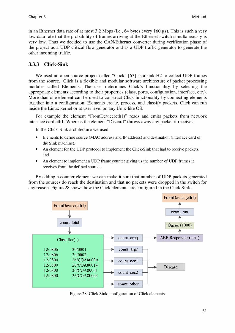
Chapter 3 Method
51
in an Ethernet data rate of at most 3.2 Mbps (i.e., 64 bytes every 160 µs). This is such a very low data rate that the probability of frames arriving at the Ethernet switch simultaneously is very low. Thus we decided to use the CAN/Ethernet converter during verification phase of the project as a UDP critical flow generator and as a UDP traffic generator to generate the other incoming traffic.
3.3.3 Click-Sink
We used an open source project called “Click” [63] as a sink H2 to collect UDP frames from the source. Click is a flexible and modular software architecture of packet processing modules called Elements. The user determines Click’s functionality by selecting the appropriate elements according to their properties (class, ports, configuration, interface, etc.). More than one element can be used to construct Click functionality by connecting elements together into a configuration. Elements create, process, and classify packets. Click can run inside the Linux kernel or at user level on any Unix-like OS.
For example the element “FromDevice(eth1)” reads and emits packets from network interface card eth1. Whereas the element “Discard” throws away any packet it receives.
In the Click-Sink architecture we used:
• Elements to define source (MAC address and IP address) and destination (interface card of the Sink machine),
• An element for the UDP protocol to implement the Click-Sink that had to receive packets, and
• An element to implement a UDP frame counter giving us the number of UDP frames it receives from the defined source.
By adding a counter element we can make it sure that number of UDP packets generated from the sources do reach the destination and that no packets were dropped in the switch for any reason. Figure 28 shows how the Click elements are configured in the Click Sink.
Figure 28: Click Sink; configuration of Click elements

Chapter 3 Method
52
3.3.4 CAN/Ethernet Converter
The prime function of a CAM/Ethernet converter is to act like a bridge between an Ethernet node and a CAN node. It must snoop every CAN message appeared on the CAN bus to which its CAN module is connected and forward that message after encapsulating it into the payload field of a UDP frame to its peer Ethernet node. The peer node could be another CAN/Ethernet converter or an Ethernet switch in our case. The bridge works as an application layer common to both CAN layer and Ethernet TCP/IP layer. Figure 29 shows how the CAN data link layer and TCP/IP stack are layered with respect to the application layer.
Application Layer
Data link Layer
Physical Layer
Transport Layer
Network Layer
Data Link Layer
Physical Layer
CAN Ethernet
Figure 29: CAN/Ethernet converter layered model
3.3.4.1 Criteria for CAN/Ethernet converter
One of the criteria was that the converter should have a CAN interface module that can support both High Speed CAN (baud rates from 40 kbps to 1 Mbps) and Low Speed/Fault Tolerant CAN (baud rates from 5 kbps to 125 kbps) to support systems running on 1 Mbps while allowing Low Speed/Fault Tolerant CAN systems to communicate over the Ethernet. The second criterion was that the converter must have an Ethernet interface enable to transmit and receive data at 10/100 Mbps (10BASE-T and 100BASE-TX) and it should perform auto negotiation (of link rate and full/half duplex mode) with the peer Ethernet node.
We choose systems that were built around ARM® microprocessors* since many of CPAC Systems products are ARM® microcontroller based. Secondly, we wanted access to the firmware that would be running inside the processor to an extent that we could use and modify the TCP/IP stack for our purposes. Moreover, we wanted minimum conversion time of Ethernet and CAN frames, which can only be done if we have access to the API of the TCP/IP stack.
Lastly, we wanted to use the CAN/Ethernet converter not only to convert CAN and Ethernet frames but also to use it as UDP packet generator with varying UDP payload size and frequency. This could only be achieved if we had access to the device’s firmware.
There are many commercial off the shelf CAN-Ethernet converters available today, such as the Tritium CAN-Ethernet bridge [64].
According to the data sheet of the Tritium CAN–Ethernet Bridge, the bridge supports Ethernet at 10/100 Mbps and a default CAN bit rate at 500 kbps. It supports bi-directional * http://www.arm.com/

Chapter 3 Method
53
CAN-Ethernet bridging using both UDP and TCP. The bridge uses UDP to broadcast messages. It uses TCP when a reliable point-to-point connection is required between the bridge and a single network device, for example when exchanging a stream of data via the CAN-Ethernet network. The bridge can only support a single TCP connection at any time.
Using the Tritium CAN–Ethernet Bridge had the downside of no access to the firmware running inside the processor used in the bridge. Additionally, as noted above it uses UDP only for broadcasting and not for unicast or point-to-point connections for which TCP is used. We wanted to use UDP not only for broadcasting messages but also for multicast and unicast messages.
For these reasons we decided to utilize a development board which has an ARM® microcontroller and built-in CAN and Ethernet interface modules. The CAN interface must support High Speed as well as Low Speed/Fault Tolerant transmission whereas the Ethernet peripheral must transfer data at 100 Mbps. Moreover we wanted to use the CAN/Ethernet converter as a UDP traffic generator as well.
We found many development boards which meet the basic requirements of the project, i.e. they have CAN and Ethernet interfaces. However, each of these boards had some drawbacks. The NetBurner Mod5282 module [65] has CAN and Ethernet interfaces that met the required specifications, but the module is built around a ColdFire 5282 microprocessor rather than an ARM® processor. The same problem occurred with Maxim's DS80C400 CAN-to-Ethernet [66] whose microcontroller utilizes the 8051 architecture.
3.3.4.2 STM32F107VC microcontroller
There exist many manufacturers who build microcontrollers based on the ARM® architecture. The STMicroelectronics* STM32F107VC microcontroller [67] incorporates the high performance ARM® Cortex™-M3 32-bit RISC core operating at 72 MHz frequency, high speed embedded memories (256 Kbytes of flash memory and 64 Kbytes of SRAM), and an extensive range of enhanced I/Os and peripherals connected to two advanced peripheral buses. It has two CAN interfaces and a 10/100 Ethernet MAC. We used the STM32F107VC development kit from IAR [68]. The development board has CAN line drivers and a 10/100 Ethernet PHY module as required to enable 10/100 Ethernet MAC communication over an Ethernet. This development board is shown in
Figure 30.
* http://www.st.com
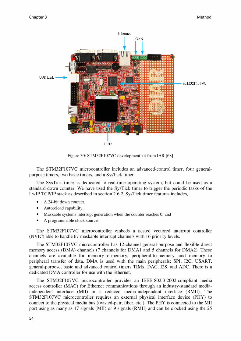
Chapter 3 Method
54
Figure 30: STM32F107VC development kit from IAR [68]
The STM32F107VC microcontroller includes an advanced-control timer, four general-purpose timers, two basic timers, and a SysTick timer.
The SysTick timer is dedicated to real-time operating system, but could be used as a standard down counter. We have used the SysTick timer to trigger the periodic tasks of the LwIP TCP/IP stack as described in section 2.6.2. SysTick timer features includes,
• A 24-bit down counter, • Autoreload capability, • Maskable systems interrupt generation when the counter reaches 0, and • A programmable clock source.
The STM32F107VC microcontroller embeds a nested vectored interrupt controller (NVIC) able to handle 67 maskable interrupt channels with 16 priority levels.
The STM32F107VC microcontroller has 12-channel general-purpose and flexible direct memory access (DMA) channels (7 channels for DMA1 and 5 channels for DMA2). These channels are available for memory-to-memory, peripheral-to-memory, and memory to peripheral transfer of data. DMA is used with the main peripherals; SPI, I2C, USART, general-purpose, basic and advanced control timers TIMx, DAC, I2S, and ADC. There is a dedicated DMA controller for use with the Ethernet.
The STM32F107VC microcontroller provides an IEEE-802.3-2002-compliant media access controller (MAC) for Ethernet communications through an industry-standard media-independent interface (MII) or a reduced media-independent interface (RMII). The STM32F107VC microcontroller requires an external physical interface device (PHY) to connect to the physical media bus (twisted-pair, fiber, etc.). The PHY is connected to the MII port using as many as 17 signals (MII) or 9 signals (RMII) and can be clocked using the 25

Chapter 3 Method
55
MHz (MII) or 50 MHz (RMII) output from the STM32F107VC microcontroller. The block diagram of the Ethernet interface is shown in Figure 31.
The Ethernet MAC interface of STM32F107VC microcontroller includes the following features:
• 10 and 100 Mbps data rates • Dedicated DMA controller allowing high-speed transfers between the dedicated SRAM and
the descriptors. • Tagged MAC frame support (i.e., VLAN support) • Half-duplex (CSMA/CD) and full-duplex operation • MAC control sub-layer (control frames) support • 32-bit CRC generation and checking/ removal • Several address filtering modes for physical and multicast addresses (multicast and group
addresses) • 32-bit status code for each transmitted or received frame. • Internal FIFOs to buffer transmit and receive frames. The transmit FIFO and the receive FIFO
are 4 Kbytes in total. • Hardware PTP (precision time protocol) support in accordance with IEEE 1588.
Figure 31: STM32F107VC Ethernet peripheral block diagram [67] The Media-independent interface (MII) defines the interconnection between the MAC
sub-layer and the PHY for data transfer at 10 Mbps and 100 Mbps. In contrast, the reduced media-independent interface (RMII) specification reduces the number of signal lines between the STM32F107VC Ethernet MAC and external PHY. According to the IEEE 802.3u standard, an MII contains 16 pins for data and control. The RMII specification reduces the pin count to 7 pins (a 62.5% decrease in pin count). The STM32F107VC development kit utilized the RMII to interface the MAC core with the PHY interface.
The CAN interface performs the following primary tasks:
• Message checking, error handling, and acknowledgement. These operations are fully handled by the CAN protocol implemented in the CAN controllers.
• Message filtering; filter and forward the received messages to the application. • Identifier recognition; once a message has passed through the filters its content must be
identified in order to compute the destination address the data must be forwarded.
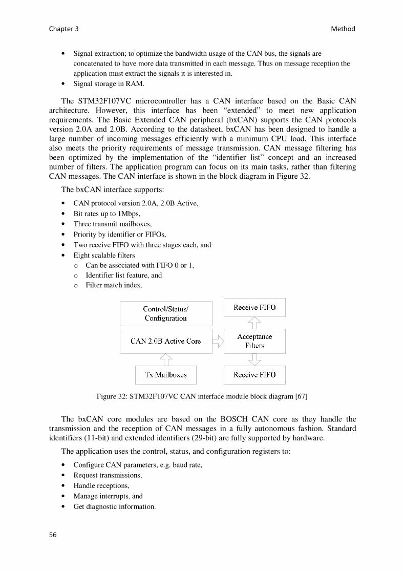
Chapter 3 Method
56
• Signal extraction; to optimize the bandwidth usage of the CAN bus, the signals are concatenated to have more data transmitted in each message. Thus on message reception the application must extract the signals it is interested in.
• Signal storage in RAM.
The STM32F107VC microcontroller has a CAN interface based on the Basic CAN architecture. However, this interface has been “extended” to meet new application requirements. The Basic Extended CAN peripheral (bxCAN) supports the CAN protocols version 2.0A and 2.0B. According to the datasheet, bxCAN has been designed to handle a large number of incoming messages efficiently with a minimum CPU load. This interface also meets the priority requirements of message transmission. CAN message filtering has been optimized by the implementation of the “identifier list” concept and an increased number of filters. The application program can focus on its main tasks, rather than filtering CAN messages. The CAN interface is shown in the block diagram in Figure 32.
The bxCAN interface supports:
• CAN protocol version 2.0A, 2.0B Active, • Bit rates up to 1Mbps, • Three transmit mailboxes, • Priority by identifier or FIFOs, • Two receive FIFO with three stages each, and • Eight scalable filters
o Can be associated with FIFO 0 or 1, o Identifier list feature, and o Filter match index.
Figure 32: STM32F107VC CAN interface module block diagram [67]
The bxCAN core modules are based on the BOSCH CAN core as they handle the transmission and the reception of CAN messages in a fully autonomous fashion. Standard identifiers (11-bit) and extended identifiers (29-bit) are fully supported by hardware.
The application uses the control, status, and configuration registers to:
• Configure CAN parameters, e.g. baud rate, • Request transmissions, • Handle receptions, • Manage interrupts, and • Get diagnostic information.

Chapter 3 Method
57
Three transmit mailboxes are provided to the software for setting up messages. The transmission scheduler decides which mailbox has to be transmitted first.
The bxCAN provides 28 scalable/configurable identifier filter banks to the application for selecting the desired incoming messages, while automatically discarding all others.
Two receive FIFOs are used by hardware to store the incoming messages. Each FIFO has three mailboxes and therefore three complete messages can be stored in each FIFO. The FIFOs are managed completely by hardware and no need for the application to handle them.
The Transmission Scheduler decides which of the three transmit mailboxes has to be transmitted first according to the priority rules. The bxCAN provides two modes for the transmit priority:
• In identifier mode when more than one transmit mailbox are pending, the transmission order is decided according to the identifiers of the messages stored in the mailboxes. The message in the mailbox with the lowest identifier value has the highest priority according to the arbitration of the CAN protocol.
• In FIFO mode the priority order is given by the transmit request order. This mode is well suited for segmented transmission.
For the reception of CAN messages, two FIFO with three mailboxes are provided. In order to minimize CPU load, ease application development, and to guarantee data consistency, the FIFO is managed completely by hardware. The application accesses the messages stored in the FIFO through the FIFO output mailbox. The extended filter mechanism avoids the application from having to perform any message filtering, thus making the CPU performance independent of the CAN bus traffic.
For the reception of CAN messages bxCAN provides two FIFOs. Each FIFO can take three complete CAN messages without CPU intervention. Each filter can be independently associated with FIFO 0 or FIFO 1, thereby reducing the real-time constraint on message reception on the application side. A block diagram of CAN message filtering is shown in Figure 33.

Chapter 3 Method
58
Figure 33: CAN message filtering and storage in STM32F107VC [67]
3.4 CAN/Ethernet Converter Application layer
As discussed in section 2.2, the CAN standard defines the two bottom layers of the OSI reference model. Use of higher layer protocols above physical and data link layers depends on the application. In the CAN/Ethernet converter we did not implement any specific higher layer protocol preferring to keep the implementation simple. The converter does not require any specific high level protocol (such as those that CPAC Systems is using in their products) instead the converter simply forwards CAN messages from one interface to the other. The only processing that is needed is to encapsulate any CAN message into a UDP datagram and vice versa. The receiving CAN nodes will interpret the message by themselves. Therefore we did not implement any higher layer protocols in our CAN/Ethernet converter.
However, in the case of Ethernet, we do need higher layer protocols, specifically network and transport, so that we can send UDP messages across the network to which the CAN/Ethernet converters are connected. For this reason we used the LwIP TCP /IP stack below the application layer and above the MAC layer of OSI reference model. The next section discuses porting the LwIP TCP /IP stack to our CAN/Ethernet converter.

Chapter 3 Method
59
3.4.1 Porting LwIP to STM32F107VC
In section 2.6.1 we have explained in detail the architecture and operation of the LwIP TCP/IP stack. In this section we explain how we ported the LwIP TCP/IP stack to STM32F107VC microcontroller.
3.4.1.1 Ethernet controller interface or network interfaces
Porting LwIP to any specific microcontroller has not been done in the official release of the LwIP. However, LwIP comes with a file called ethernetif.c, which works as an interface between the LwIP TCP/IP stack and the Ethernet MAC interface. This file acts as a template to be filled-in in order to develop an Ethernet network interface driver for a specific microcontroller. The ethernetif.c file contains functions that ensure the transfer of the frames between the low-level network interface driver and the LwIP stack. Its main function is ethernetif_input( ), which is called when a packet is ready to be read from the interface. When the Ethernet controller receives a valid frame, it generates an interrupt in the handling function which invokes the ethernetif_input( ) function.
3.4.1.2 Periodic Tasks
There are a number of internal tasks for different purposes, such as updating ARP entries in the ARP table and other TCP facilities in the LwIP TCP/IP stack that should be called periodically. Even when application program uses only UDP, the stack requires a timer. For this timer we used the STM32F107VC SysTick timer. The SysTick is used to build a system clock that serves as a reference to call various tasks at regular intervals. LwIP_Periodic_Handle( ) is the main function defined in the netconf.c file and this function is called whenever the SysTick timer overflows. This function guarantees the periodic dispatch of LwIP tasks.
3.4.1.3 Configuration of the LWIP protocol stack
As discussed in section 2.6.1, LwIP allows configuration of the size of the heap, number of pbuf structures, and the number of PCB. There are no special rules to follow because these parameters primarily depend on the application itself. The following main parameters are important to configure:
• Protocol selection, such as DHCP, which can be enabled or disabled, as defined by LWIP_DHCP
• The maximum number of simultaneously active connections, for TCP this is defined by MEMP_NUM_TCP_PCB and for UDP by MEMP_NUM_UDP_PCB
• The heap size, defined by MEM_SIZE • The number of buffers, defined by PBUF_POOL_SIZE, and the buffer size, defined by
PBUF_POOL_BUFSIZE
The number of buffers and the heap size allocated to the application depend on the number of simultaneous connections required by the application and the available amount of RAM. These configuration paramters affect the performance of the application. Increasing the number of buffers and heap size boost the performance at the cost of RAM, leaving less space for the main application. In contrast, decreasing these parameters increases the available RAM, but will still limit the application’s performance due to the limitations of the specific LwIP configuration.

Chapter 3 Method
60
The various pbuf memory options parameters are shown in Table 5. The other parameters are described in the other tables. The default values of these parameters can be found in the opt.h file. A new file with modified values was defined based on the opt.h file.
Table 4: Memory Option Settings for LwIP Option Name Description
MEM_SIZE The size of the heap. If the application sends a lot of data that needs to be
copied, this is set high.
MEMP_NUM_PBUF
The number of memp struct pbufs (used for PBUF_ROM and PBUF_REF).
If the application sends a lot of data out of ROM (or other static memory),
this is set high.
MEMP_NUM_UDP_PCB The number of UDP protocol control blocks. One per active UDP
"connection."
Table 5: Pbuf Memory Options Configuration
Attribute Description
PBUF_POOL_SIZE Number of buffers in pbuf pool.
PBUF_POOL_BUFSIZE Size in bytes of each pbuf in pbuf pool.
Table 6: IP Options Configuration Parameters Attribute Description
IP_FORWARD
Set to 1 for enabling ability to forward IP packets across
network interfaces. To run LwIP on a single network interface,
this is set to 0.
IP_REASSEMBLY Reassemble incoming fragmented IP packets.
IP_FRAG Fragment outgoing IP packets if their size exceeds MTU.
Table 7: DHCP Options Configuration Parameters Attribute Description
LWIP_DHCP Is DHCP required?
DHCP_DOES_ARP_CHECK Do an ARP check on the offered address.
Table 8: ICMP Options Configuration Parameters Attribute Description
LWIP_ICMP Is ICMP required?
ICMP_TTL ICMP Time To Live value
Table 9: UDP Options Configuration Parameters Attribute Description
LWIP_UDP Is UDP required?
UDP_TTL UDP Time To Live value
3.4.1.4 Raw API functions for UDP interface
The raw API provides direct access to the LwIP TCP/IP stack and avoids extra buffering and message passing features. Asynchronous network events (data received, connection

Chapter 3 Method
61
established, etc.) are communicated to the application through callback functions. The pointer to the callback is defined during the initialization of the UDP socket using the raw API. Table 10 lists the event and associated callback routine.
Table 10: UDP Events, Callbacks, and Routine to register callback events Event Callback Routine
UDP Data Received *recv( ) udp_recv ( )
void* udp_init (void) Initializes the LwIP stack.
struct udp_pcb *udp_new (void) Creates a new UDP PCB used for UDP
communication. The PCB is not active until it has either been bound to a local address or connected to a remote address.
void udp_remove (struct udp_pcb *pcb) Removes and deallocates the PCB.
err_t udp_bind (struct udp_pcb *pcb, struct
ip_addr *ipaddr, u16_t ort)
Binds a PCB to a local address. The IP-address argument "ipaddr" is the local IP address of the network interface.
err_t udp_connect (struct udp_pcb *pcb,
struct ip_addr *ipaddr, u16_t port)
Sets the remote end of a PCB. This function does not generate any network traffic, but only set the remote address in a PCB. The IP-address argument "ipaddr" could be a unicast or a broadcast address.
err_t udp_disconnect (struct udp_pcb *pcb) Removes the remote end of a previously defined PCB. This function does not generate any network traffic, but only removes the remote address of a PCB.
err_t udp_send (struct udp_pcb *pcb, struct
pbuf *p)
Sends the pbuf p from the PCB bind to a local address to the remote end connected to that PCB. The pbuf memory is not freed even after sending.
void udp_recv (struct udp_pcb *pcb, void (*
recv)(void *arg, struct udp_pcb *upcb, struct
pbuf *p, struct ip_addr *addr, u16_t port),
void *recv_arg)
Specifies a callback function that will be called by the LwIP when a UDP datagram is received.
3.4.1.5 System initialization
Before we use functions from the raw API, we have to call various LwIP functions in a specific order shown below,
stats_init ( ) Clears the structure where runtime statistics are gathered. sys_init ( ) Initializes the OS emulation layer. Not in our case. mem_init ( ) Initializes the dynamic memory heap defined by MEM_SIZE. memp_init ( ) Initializes the memory pools defined by MEMP_NUM_PBUF. pbuf_init ( ) Initializes the pbuf memory pool defined by PBUF_POOL_SIZE. etharp_init ( ) Initializes the ARP table and queue of outgoing packets for
unknown address. udp_init ( ) Clears the UDP PCB list.

Chapter 3 Method
62
Now the LwIP stack is completely initialized, but before starting a UDP session or TCP connection, a few functions (described below) are needed to be called at regular intervals. Also a network device must be registered and enabled.
netif_add ( ) Adds our network interface to the netif_list. netif_set_default ( ) Registers the default network interface. netif_set_up ( ) When the network interface is fully configured
this function is called. dhcp_start ( ) Creates a new DHCP client for this interface
on the first call.
3.4.2 Application layer firmware
The firmware for the application layer is part of a main program that not only acts as an application layer for CAN and Ethernet interface, but also initializes and controls the STM32F107VC microcontroller resources including clock, timers, and peripherals. It manages the CAN and Ethernet interfaces which includes the initialization of the CAN and Ethernet modules, management of the CAN and Ethernet interrupts and execution of the LwIP periodic tasks. We used IAR Embedded Workbench for ARM® integrated development environment [69] which has C/C++ compiler that we used to write and compile the main program, i.e., the application layer, and the ported LwIP TCP/IP stack of CAN/Ethernet converter.
After a reset, the main program starts by initializing the clocks, nested vector interrupts, Ethernet MAC, DMA, and CAN interface. Moreover, the code configures the ports as digital or analog and input or output. Initialization of the CAN interface involves configuring the CAN bus data rate (a standard fix bit rate such as 1 Mbps, 125 kbps, etc.), setting the mode of operation, and the configuration and scaling of identifier and filters. Since we wanted to make CAN/Ethernet transparent, we configured the filters and identifiers such that it should receive every CAN message with any identifier appearing on the CAN bus.
After the initialization of modules and peripherals, the main program calls the LwIP initialization function which calls several functions to initialize the LwIP TCP/IP stack so that it is ready to receive and forward messages from the application layer and the MAC layer. This initialization has been described in the previous section. Some of the many initial tasks of LwIP are the creation of a memory heap and pool, assignment of a MAC address to the interface, and acquisition of an IP address for the CAN/Ethernet converter using DHCP. To get an IP address LwIP sends a DHCP request to the peer Ethernet node requesting a dynamically assigned IP address. It makes for a certain number of requests and waits for a reply. If it does not get an IP address from the DHCP server, then assigns a static IP address to the CAN/Ethernet converter board. Note that when compiling the code we must configure a unique default IP address and a unique MAC address for each CAN/Ethernet converter.
Once the board has been assigned either a dynamic or a static IP, the main program calls the UDP client/server application layer which first initializes a UDP client and a server. The initialization includes creation of UDP PCB (discussed in section 3.4.1), binding of IP address with a UDP socket and declaration of the UDP callback function.
After that the main programs enters an infinite loop where timer interrupts cause it to periodically calls the LwIP periodic tasks. The application layer waits for either a CAN interrupt from the CAN data link layer or an Ethernet interrupt from the transport layer (via the callback function). When the CAN module receives a compete CAN message it generates an interrupt informing the application layer to retrieve the message from the CAN Receive

Chapter 3 Method
63
FIFO. The application layer reads this message and encapsulates it into UDP datagram of payload size 22 bytes then sends it to the LwIP TCP/IP stack with the client port number and the converter's IP address.
When the LwIP TCP/IP stack receives a UDP datagram, it calls the callback function previously assigned with a UDP PCB and a UDP socket. Now the application retrieves the message from the pbuf and places it into the CAN transmit FIFO or mailbox from where the CAN data link layer transmits it on the CAN bus.
Figure 34 show the data flow of the main and application layer codes of the CAN/Ethernet converter respectively.
Figure 34: Flow chart of main program
3.4.3 CAN/Ethernet converter as UDP traffic generator
As discussed in section 3.3.2, we decided to use CAN/Ethernet converter not only as a converter but also as UDP traffic generator. That is traffic generator function is in addition the basic functionality of a CAN/Ethernet message conversion. As UDP traffic generator the device can output UDP datagrams with varying payload sizes and at data rates. We programmed the application layer to transmit UDP packets in Ethernet frames of sizes 64 bytes, 514 bytes, 1014 bytes, and 1514 bytes. Moreover we programmed it to send UDP packets at different data rates depending on the number of sources that we wanted to emulate. The main code remained the same except for a few changes described below.
The initialization procedure and configuration of modules and peripherals following the reset remained the same. Once the board has been assigned either a dynamic or a static IP,

Chapter 3 Method
64
and the UDP client/server are initialized with binding of UDP PCB to local IP address and port, the board is ready to transmit UDP packets of any size at given data rate.
To increase the probability of frames arriving simultaneously to the switch, we set the data rates of the two boards slightly differently. We chose the value of the variable that determined the data rate from prime numbers as described in section 3.3.1. Moreover we wanted to trigger both boards simultaneously to enable the two converters to transmit same number of packets. To do this we used a PCAN-USB interface attached to a personal computer (PC). We connected the two CAN/Ethernet converter boards and the PCAN-USB to a common CAN bus. In this way both CAN/Ethernet converters receive CAN-trigger messages (sent by the PC on the CAN bus) nearly simultaneously and both start transmitting UDP datagrams concurrently.
When the application layer of the CAN/Ethernet converter board receives a CAN message, it encapsulates that message into a UDP payload field of 22 bytes, 472 byes, 972 bytes, or 1472 bytes depending on the measurement setup. It continues to send the same UDP packet at the data rate defined for certain duration or for a given number of UDP packets. Figure 35 shows the flow of data at application layer of the CAN/Ethernet converter.
Figure 35: Flow chart of application layer
3.5 Net analyzer
To measure the forwarding time from the moment when a UDP frame starts to appear on the Ethernet cable (or enters the switch port) to the instant when the UDP frame is completely received by the sink, we need a hardware which can time-stamps the UDP frame at the two instants above. This device should generate a time stamp when it first sees a UDP frame entering the switch and again when it sees a UDP frame leaving the switch. Also it should not take too much time in order to avoid negatively affecting the forwarding itself.
For the purpose of time-stamp we used a dedicated network interface card or network analyzer that not only time-stamps Ethernet frames while they traverse the Ethernet network but also saves these frames to the hard disk of the PC where the interface card is installed. The Hilscher Gesellschaft für Systemautomation mbH network analyzer card netANALYZER NXANL 50-RE [70] works as a passive component in a real-time Ethernet system to record and analyze the data traffic.

Chapter 3 Method
65
3.5.1 Connecting the analyzer card to capture traffic
The netANALYZER card has two Test Access Points (TAP) named TAP A and TAP B. Both TAPs have two bidirectional full-duplex Ethernet ports (TAP A port 0/1, TAP B port 2/3). Ethernet frames entering a port are time-stamped and forwarded to the corresponding egress port. For example a frame which enters TAP A port 0 will leave from TAP A port 1 and vice versa. Figure 36 shows how Ethernet devices are connected to the netANALYZER card.
Figure 36: netANALYZER card simultaneously sniffing two Ethernet links
The netANALYZER card stores the data via direct memory access to the hard disk of the PC. Subsequently the netANALYZER software converts the stored binary files (*.hea) into the open WinPcap format (*.pcap), which can be analyzed with Wireshark or other applications that can process pcap files. The netANALYZER can be used in either of its two modes : Data-capture or Timing analysis mode. In the data-capture mode the Ethernet frames are captured, time-stamped, and recorded to the hard disk of the PC. In the timing analysis mode (Timing Analysis) no Ethernet frames are stored, only the time-stamped frames are analyzed.
3.5.2 Time-stamps
The time stamp is taken at the reception of the SFD (start-of-frame delimiter). This means that the netANALYZER time-stamps an Ethernet frame after its SFD has entered either TAP A or TAP B. This means that the netANALYZER card misses the serialization time of the first eight bytes (preamble and SFD) of an Ethernet frame. However, in calculating the forwarding time; only the difference in time between when a frame appears at the two TAPs (TAP B-TAP A) is relevant, hence the affect is nullified. Figure 37 shows when the netANALYZER time-stamps an incoming Ethernet frame.

Chapter 3 Method
66
Figure 37: Time-stamping in netANALYZER (Source [70])
3.5.3 Graphical User Interfaces
The data capture is configured and started via the netANALYZER software. Once started the card and the software capture and save the frames of the communication lines on the hard disk. Figure 38 shows the GUI of the netANALYZER software.
Figure 38: netANALYZER software (GUI)
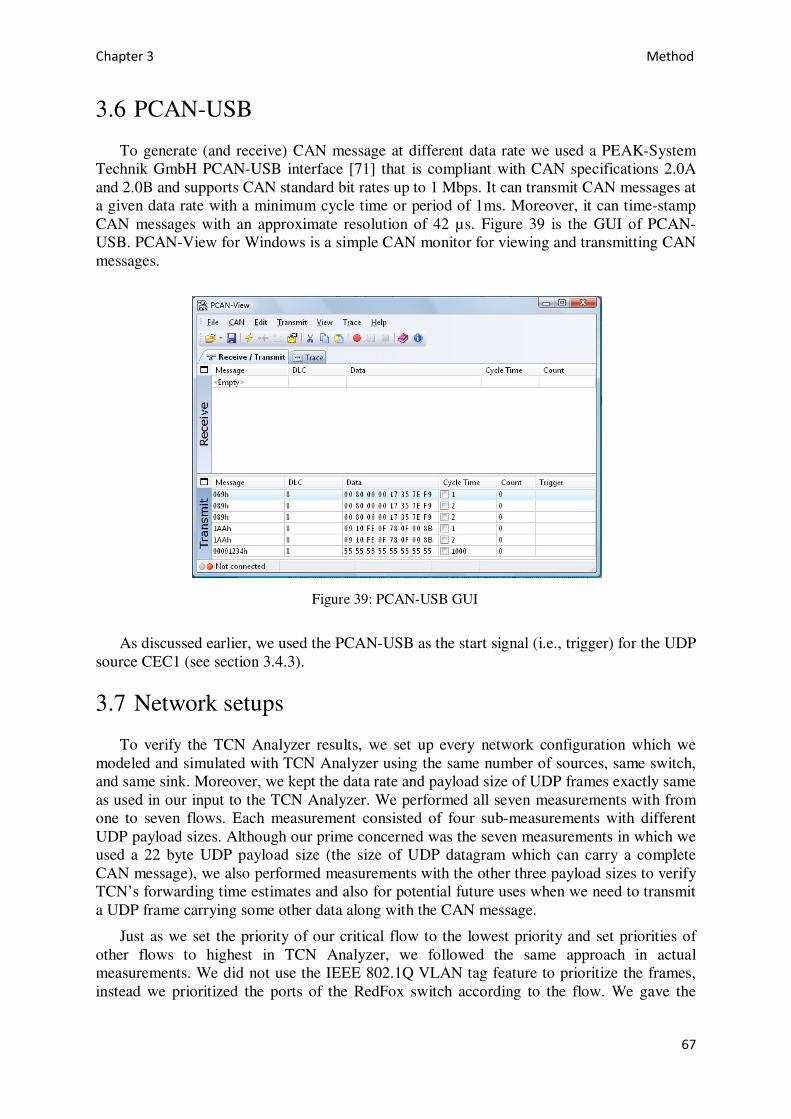
Chapter 3 Method
67
3.6 PCAN-USB
To generate (and receive) CAN message at different data rate we used a PEAK-System Technik GmbH PCAN-USB interface [71] that is compliant with CAN specifications 2.0A and 2.0B and supports CAN standard bit rates up to 1 Mbps. It can transmit CAN messages at a given data rate with a minimum cycle time or period of 1ms. Moreover, it can time-stamp CAN messages with an approximate resolution of 42 µs. Figure 39 is the GUI of PCAN-USB. PCAN-View for Windows is a simple CAN monitor for viewing and transmitting CAN messages.
Figure 39: PCAN-USB GUI
As discussed earlier, we used the PCAN-USB as the start signal (i.e., trigger) for the UDP source CEC1 (see section 3.4.3).
3.7 Network setups
To verify the TCN Analyzer results, we set up every network configuration which we modeled and simulated with TCN Analyzer using the same number of sources, same switch, and same sink. Moreover, we kept the data rate and payload size of UDP frames exactly same as used in our input to the TCN Analyzer. We performed all seven measurements with from one to seven flows. Each measurement consisted of four sub-measurements with different UDP payload sizes. Although our prime concerned was the seven measurements in which we used a 22 byte UDP payload size (the size of UDP datagram which can carry a complete CAN message), we also performed measurements with the other three payload sizes to verify TCN’s forwarding time estimates and also for potential future uses when we need to transmit a UDP frame carrying some other data along with the CAN message.
Just as we set the priority of our critical flow to the lowest priority and set priorities of other flows to highest in TCN Analyzer, we followed the same approach in actual measurements. We did not use the IEEE 802.1Q VLAN tag feature to prioritize the frames, instead we prioritized the ports of the RedFox switch according to the flow. We gave the

Chapter 3 Method
68
lowest priority of “0” to the port where we connected the critical flow CEC1 and the highest priority of “7” to the remaining ports connected traffic generators.
3.7.1 Single flow
We began the evaluation and verification with single flow, i.e. there was only one CAN/Ethernet Converter, CEC1 generating UDP frames to one sink H2. As shown in Figure 40 the CEC1 is connected first to the TAP A port 0 of netANALYZER and then the TAP A port 1 is connected to port 1 of the RedFox switch. Whenever CEC1 generated a UDP frame destined to the sink H2, the netANALYZER time-stamped that frame on its way to the switch. Also, the connection between port 7 of RedFox switch and sink H2 also passes through the netANALYZER so that the netANALYZER can time-stamp the egress frames destined to H2. In this way the frames coming from port 2 and heading towards H2 were time-stamped in the netANALYZER before they reached H2.We set the ingress and egress link speeds of all components in the network including the netANALYZER to 100 Mbps full duplex mode.

Chapter 3 Method
69
Figure 40: Ethernet network setup for the evaluation of one flow case
We configured the CAN/Ethernet converter so that we can take four different measurements with UDP payload lengths 22 bytes, 472 bytes, 972 bytes, and 1472 bytes in this single flow setup. Table 11 shows the UDP frame size, payload size, and corresponding data rate set in the CAN/Ethernet converter.
Table 11: Parameters set in CAN/Ethernet converter for one flow
No. of Flows Frame size / Payload size Data rate
(Bytes / Bytes) (Mbps)
1 x CEC1
64 / 22 0.512
514 / 472 4.112
1014 / 972 8.112
1514 / 1472 12.112

Chapter 3 Method
70
We performed the four measurements according to the data rate and UDP frame sizes as discussed above for certain duration. The netANALYZER stored every frame it received after time-stamping at the incoming ports of TAP A and TAP B. At the same time we counted in H2 the number of received UDP frames from CEC1.We will analyze the measured forwarding time in this scenario in Chapter 4.
3.7.2 Two flows
We increased the number of flows to two through the Ethernet switch just as we did when we were modeling the network with TCN Analyzer. Figure 41 shows the two flows setup. Here CEC1 is generating the critical flow whose upper bound on forwarding time was previously estimated by TCN Analyzer. The other flow generated is by CEC2 (a second CAN/Ethernet converter acting as a traffic generator) is the non-critical flow acts as traffic to create delay for the critical flow CEC1 in the switch.
We linked the critical flow source CEC1 in the same way we did in single flow setup. We linked traffic generator CEC2 to port 2 of RedFox switch. Sink H2 was connected in the same way as in the case of a single flow. Here the netANALYZER time-stamps the UDP frames from CEC1 at TAP A port 0 and TAP B port 2 and also the CEC2 frames at TAP B port 2. In this way we would know when CEC2 and CEC1 arrived at the switch with reference to a common time-stamp and also if they had arrived at their respective ports simultaneously. This would make it easy to visualize near simultaneous arrivals if they occur as per our assumption on the probability of their occurrence. Figure 41 shows the CAN/Ethernet network setup for the evaluation of two flows scenario.

Chapter 3 Method
71
Figure 41: Ethernet network setup for the evaluation of two flows case
We set the ingress and egress link speeds of all components in the network to 100 Mbps. Moreover, we used the IEEE 802.1p port priority feature, as the RedFox switch is IEEE 802.1Q compliant switch, and set the priority of port 1 where the critical UDP flow source CEC1 is connected to “0” and priority of port 2 where UDP traffic source CEC2 is connected to “7”.
We configured both CEC1 and CEC2 CAN/Ethernet converters for four different measurements with UDP payload lengths 22 bytes, 472 bytes, 972 bytes, and 1472 bytes in this two flows setup. Table 12 shows the UDP frame size, payload size, and corresponding data rate set in each CAN/Ethernet converter.
Table 12: Parameters set in CAN/Ethernet converter for two flows
No. of Flows Frame size / Payload size CEC1 Data rate CEC2 Data rate
(Bytes / Bytes) (Mbps) (Mbps)
1 x CEC1
+
1 x CEC2
64 / 22 5.09 5.05
514 / 472 33.07 31.84
1014 / 972 33.35 32.90
1514 / 1472 38.46 37.28
Chapter 3 Method
72
The data rate of both CEC1 and CEC2 are set according to the assumptions we stated in section 3.3.1. That is we used the highest data rate possible under the constraint that the sum of ingress data rates should not exceed the egress link rate. This was to make sure no packet would be dropped in the switch due to queuing and overloading of the switch memory. This is the same constraint we maintained while we modeled the network in TCN Analyzer.
We performed the four measurements according to the data rate and UDP frame sizes for specific duration. The duration was not deterministic, but rather we stopped each measurement when we saw H2 had received enough UDP frames (around 50,000). We observed through these experiments that (nearly) simultaneous arrivals occurred for this number of transmitted UDP frames. The netANALYZER recorded onto the hard disk the frames it received after time-stamping them at incoming ports of TAP A and TAP B. The traffic to H2 included frames from CEC1 as well as from CEC2. Moreover we checked in H2 the number of received UDP frames from CEC1 and CEC2 separately.
3.7.3 Four flows
With four flows the procedure was same as with two flows. However, since we only had two converter boards where one board was used to transmit the critical flow while the second was used to generate traffic, we modified the network. Rather than use a third and fourth converter board as traffic generators we use a single board CEC2 as a traffic generator and configured a second RedFox switch to act as a repeater for traffic coming in from one port to output this traffic on 3 ports. These ports where then connected as input to the original RedFox switch.
Although the three links from the second switch are redundant and one might think that the switches would not allow redundant links in between them. We played a trick and did not allow the RedFox switch 2 to learn the MAC address of H2 (A switch stores in its memory the port where an Ethernet node is connected based upon its MAC address) by not allowing H2 to send any messages to CEC2. We restricted H2 not to send even an ARP message to CEC2 during the measurement. However, when an Ethernet node first starts to send IP packets to another node it first sends an ARP message to learn the mapping between the destination IP address and MAC address. We managed to make H2 to send ARP message to CEC2 before we began the measurement by temporarily connecting H2 and CEC2. We sent PING messages from H2 to CEC2 to let them learn each other’s MAC addresses. By doing so we could avoid the transmission of ARP messages from CEC2 and H2 to each other during the measurements. It is to be noted that during the measurement H2 never sent any message back to CEC1 or CEC2 except for ARP messages.
However, we let the RedFox switch 1 to learn the MAC address of CEC1 and H2. While H2 and CEC2 were connected to RedFox switch 1 (whereas the RedFox switch 2 was kept aside and was not connected to RedFox switch 1), we sent PING message from H2 to CEC1. In this way the H2 and CEC1 learned each other’s MAC addresses and also the RedFox switch 1 knew to which ports CEC1 and H2 are connected.
At this point the RedFox switch 1 knew to which of its ports CEC1 and H2 were connected. While RedFox switch 2 only knew the port to which CEC2 was connected. To be on the safe side we also disabled the RSTP in both RedFox switches. Therefore, although there were redundant links in between the two switches, the ARP message deception as explained above and disabling RSTP prevented the RedFox switches from knowing about the redundant links.

Chapter 3 Method
73
When the RedFox switch 2 received frames at port 1, it broadcast those frames to its remaining ports as it did not know to which ports the destination node (H2) is connected. RedFox switch 2 then acted like a repeater. This had an obvious advantage that all the outgoing frames would arrive simultaneously at their corresponding RedFox switch 1ports resulting in an increased probability of frame arriving simultaneously at RedFox switch 1.
Although the RedFox switch 1 was receiving frames on its ports from the same source simultaneously, it simply forwarded them all to the port where H2 was connected as it knew the port and MAC address of H2. Figure 42 shows the CAN/Ethernet network setup for the evaluation of the four flows scenario.
Figure 42: Ethernet network setup for the evaluation of four flows case
We set the ingress and egress link speeds of all components in the network including the RedFox Switch 2 to 100 Mbps and full duplex mode. Moreover we set the priority of port 1 where critical UDP flow source CEC1 was connected to “0” and priority of port 2, port 3, and port 4 where noise traffic frames from CEC2 were arriving through RedFox switch 2 to “7”. In the RedFox switch 2 all ports had equal priorities.
The configuration of CEC1 and CEC2 CAN/Ethernet converters was same for the previous scenarios. Table 13 shows the UDP frame size, payload size, and corresponding data

Chapter 3 Method
74
rate set in each CAN/Ethernet converter. Again, data rates of both CEC1 and CEC2 were set here according to the assumptions we have made in section 3.3.1.
Table 13: Parameters set in CAN/Ethernet converter for four flows scenario
No. of Flows Frame size / Payload size CEC1 Data rate CEC2 Data rate
(Bytes / Bytes) (Mbps) (Mbps)
1 x CEC 1
+
3 x CEC 2
64 / 22 14.44 14.21
514 / 472 17.52 18.75
1014 / 972 17.43 17.99
1514 / 1472 17.51 18.00
We performed the four measurements according to the data rate and UDP frame sizes for a specific number of frames. We stopped the measurement when we had enough measurements of frames that arrived simultaneously. We checked in H2 that the number of received UDP frames from CEC2 was approximately four times that of CEC1.
3.7.4 Seven flows
Finally we performed measurements in which we activated all available ports of the RedFox Switch 1. The configuration of ports, data rate, payload sizes, and other aspects remained the same. Figure 43 shows the setup for seven flows. CEC1 and CEC2 were configured according to the data rates in table 14.
Table 14: Parameters set in CAN/Ethernet converter for four flows scenario
No. of Flows Frame size / Payload size CEC1 Data rate CEC2 Data rate
(Bytes / Bytes) (Mbps) (Mbps)
1 x CEC1
+
6 x CEC2
64 / 22 14.44 14.20
514 / 472 10.32 10.00
1014 / 972 10.01 9.97
1514 / 1472 10.12 9.94

Chapter 3 Method
75
Figure 43: Ethernet network setup for the evaluation of seven flows case
3.8 CAN/Ethernet conversion time
In order to replace a CAN bus with an Ethernet in steer by wire applications, it was important to study not only the latency in Ethernet network, but also the time a CAN/Ethernet converter took to convert a CAN message into an Ethernet frame and vice versa (This was represented as Tconv in Figure 1on page 6). Although this conversion time will depend on the internal architecture of the converter and its processing capabilities, here we present a test setup we used to calculate the CAN/Ethernet conversion time of the STM32F107VC development board.
There were two methods to calculate the forwarding time. One was to let the converter itself calculate the CAN to Ethernet and Ethernet to CAN conversion time. We could use the timers available in STM32F107VC (such as the SysTick clock). The timer had to be triggered when the interrupt was generated for a received CAN message and stopped when the MAC core generated an interrupt that the Ethernet frame had been send. The same procedure could be followed when the MAC core generated an interrupt for a received Ethernet frame and when the CAN peripheral sent the CAN message. The drawback in this method was the overhead that this code would add to the conversion time.

Chapter 3 Method
76
The second method was easy and did not require extra code. Figure 43 shows the connections of the components used to calculate the CAN/Ethernet conversion time and also the delays that occurred in this setup.
Figure 44: Setup to calculate CAN/Ethernet conversion delay. Also shown are the delays that occurred in this setup. (Delays shown as boxes are not drawn to scale).
As shown in the Figure 43, we connected the network interface card of a PC to the TAP A port 0 of netANALYZER and TAP A port 1 to the Ethernet interface of our CAN/Ethernet converter CEC1. In the PC we installed and used software called Comm Operator Pal [72] which generates UDP frames of given data size and rate. We set up a CAN bus in between the two CAN/Ethernet converters and PCAN-USB. This was to make sure that what PC was transmitting would appear in the PCAN-USB Viewer. The second converter CEC2 received the CAN message and sent it to our sink H2 via netANALYZER TAP B.
Using the above setup and taking the difference of time-stamps TAP B and TAP A gave us the sum of the Ethernet serialization delay in between PC/Comm Operator Pal and CEC1, Ethernet to CAN conversion delay in CEC1, CAN serialization delay in between CEC1 and CEC2, and CAN to Ethernet conversion delay in between CEC2 and H2.
The measured Ethernet to CAN conversion delay and CAN to Ethernet conversion delay would give us an accurate value of the CAN/Ethernet conversion time of our CAN/Ethernet convertor. We will use this CAN/Ethernet conversion delay to compute an end-to-end delay in our proposed CAN/Ethernet network in chapter 4.
3.9 Validation on the test rigs
As said earlier in the introduction of this chapter, we added a third phase of validation in our methodology after establishing feasibility in the first two phases. Here we linked our

Chapter 3 Method
77
CAN/Ethernet network with an existing CAN network of CPAC Systems and performed the tests on two test rigs: single driveline and twin driveline. Figure 45 shows the location of CAN nodes in a typical boat. The boat has twin driveline systems common to both port side and starboard side. The most critical CAN bus that needs to be replaced in the future with Ethernet is the one which is running from HCU (Helm Control Station) to PCU (Power Train Control Unit). As shown in Figure 45, the HCU is located near to the steering wheel unit whereas the PCU is located near the boat’s engines. The distance between these two increases with the increase in the size of boats, ship, and other vessels.
Figure 45: CAN Nodes and Bus locations in a typical boat [Courtesy of Volvo Penta]
3.9.1 Single driveline
In this test setup we used the single driveline systems as shown in Figure 46. We broke the CAN bus running from PCU to HCUs and inserted the two CAN/Ethernet converters along with the Ethernet switch as shown in the Figure 47. The only modification required in the CAN/Ethernet converter’s application firmware was the change of CAN bus rate. We changed the CAN link rate from 1Mbps to 125kbps for the electronic vessel control (EVC) bus. We performed the test according to the standard procedures which CPAC Systems follows to certify the correctness of their systems. The acceptance criteria and test results will be discussed in section 4.10.

Chapter 3 Method
78
Figure 46: EVC Single engine installation with dual helm station ECU diagram (single helm installation) [Courtesy of CPAC Systems]
Figure 47: EVC Single engine installation with dual helm station with CAN-Ethernet Converters
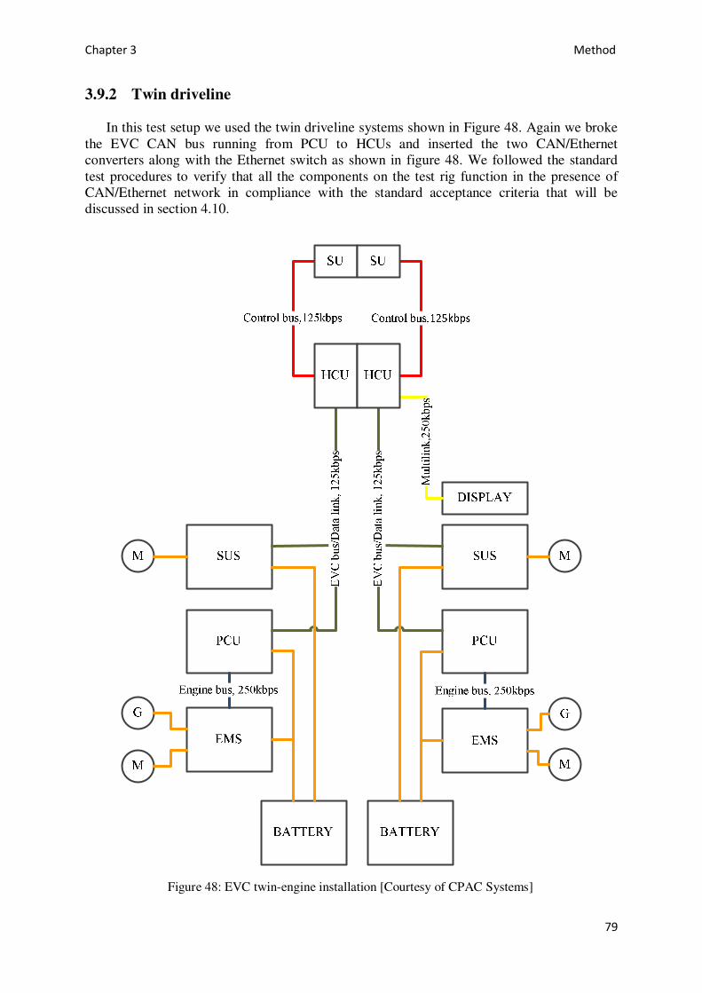
Chapter 3 Method
79
3.9.2 Twin driveline
In this test setup we used the twin driveline systems shown in Figure 48. Again we broke the EVC CAN bus running from PCU to HCUs and inserted the two CAN/Ethernet converters along with the Ethernet switch as shown in figure 48. We followed the standard test procedures to verify that all the components on the test rig function in the presence of CAN/Ethernet network in compliance with the standard acceptance criteria that will be discussed in section 4.10.
Figure 48: EVC twin-engine installation [Courtesy of CPAC Systems]
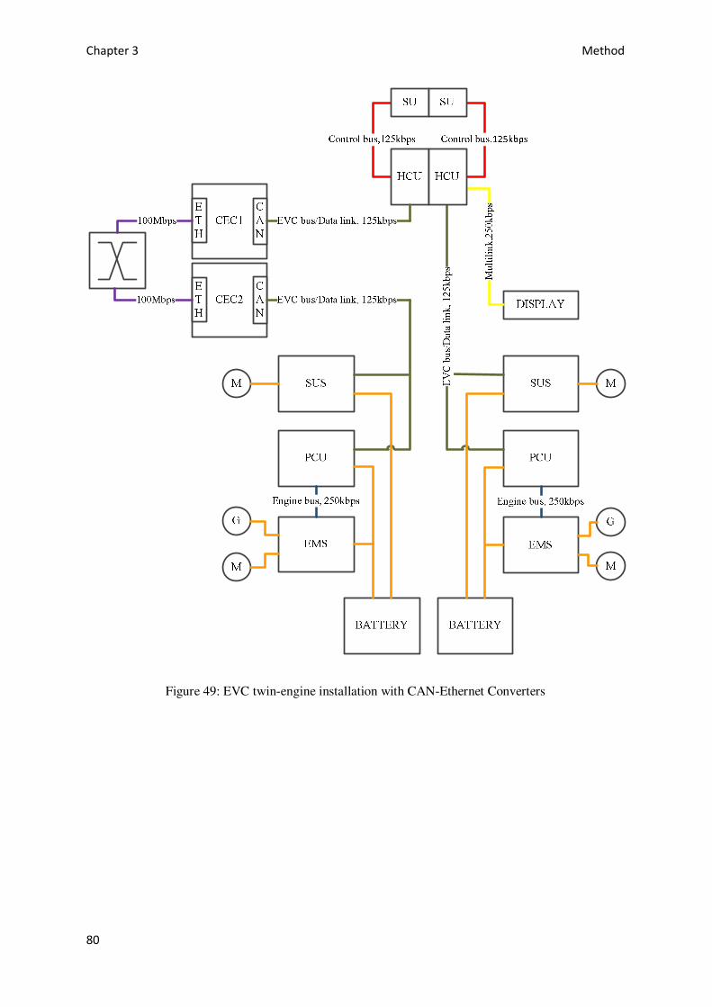
Chapter 3 Method
80
Figure 49: EVC twin-engine installation with CAN-Ethernet Converters
4 Analysis This chapter analyzes the results obtained from the method followed in chapter 3. Section
4.1 presents the estimates made by TCN Analyzer on the upper bounds on the worst case latencies in all the Ethernet networks modeled and analyzed. Section 4.2 shows the results obtained with measurements using the prototype converters as described in chapter 3. Section 4.3 discusses the problem of netANALYZER with respect to its timestamp operation. Section 4.4 presents the results of the practical measurement for the case of single flow, section 4.5 presents the results for the case of seven flows, and section 4.6 presents the practical verification results of all 28 measurements performed in the second phase of this project.
Section 4.7 compares the results from theoretical evaluation and practical evaluation. It comments on these results and analyzes if practical evaluation was below or above the upper bound estimation made using TCN Analyzer. Section 4.8 examines the CAN/Ethernet conversion time as calculated using the method described in chapter 3. Section 4.9 discusses the Ethernet bandwidth utilization in the proposed CAN/Ethernet network. Finally section 4.10 presents the results of the validation tests performed on the CPAC Systems tests rigs as was described in section 3.9.
4.1 Theoretical evaluation: modeling and simulation
This section presents the results of the theoretical evaluation carried out using TCN Analyzer. As described in chapter 3, we modeled the Ethernet networks using TCN Analyzer according to the requirements and proposed use of the CAN/Ethernet network by CPAC Systems. We configured a network using a single Ethernet switch and tried to create worst case conditions for a UDP frame carrying a CAN message, in order to estimate the worst case delay or (i.e., maximum forwarding time) that a frame could experience while traversing the network from the source to the switch and to the destination.
As stated in chapter 3, we performed the modeling with various setups; one source generating UDP frames destined to one sink/ destination, two sources (one critical source and one interfering source) generating UDP frames destined to one sink, and so on up to seven sources (one critical source and six additional traffic sources) generating UDP frames destined to the same single sink. We stopped at seven sources since there were only eight ports available on RedFox switch that we used. Moreover, in each of the seven estimates we examined four sub-cases with different Ethernet frame sizes, from the smallest (64 bytes) to 1514 bytes. Refer to section 3.1 for more details on the method.
We expected that TCN Analyzer would give us an upper bound on the forwarding time for the critical frame in each case based on the hypothesis we made concerning latencies in switched Ethernet. The sources of latency which we described in section 3.1 include store and forward latency (as we used a store-and-forward switch), switch fabric processing latency or switch internal routing delay, wireline or propagation delay, queuing latency, blocking latency and interference latency. We anticipated that the TCN Analyzer would give us the total worst case delay a UDP frame in the critical flow could suffer by taking into account all of these sources of latency.
Table 15 shows the upper bound on the worst case forwarding time (latency) as estimated by TCN Analyzer for various numbers of flows, from one flow to seven flows, across the RedFox Ethernet switch 1. The sub-cases utilized 64 bytes, 514 bytes, 1014 bytes, and 1514 bytes as the lengths of the Ethernet frames with UDP payload size of 22 bytes, 472 bytes, 972

Chapter 4 Analysis
82
bytes, and 1472 bytes respectively. In each measurement CEC1 is the critical UDP flow whose frames were supposed to carrying the CAN message. On the other hand CEC2 is also generating UDP flow, this traffic is destined to the same output port so that it generates additional delay for the critical flow CEC1.
The mnemonic 1x CEC1 means that there was only one flow, the critical flow, entering
the RedFox switch 1 at one of its ports as modeled in TCN Analyzer. The mnemonic 1x CEC2 means that there was only one source of additional UDP traffic used in the modeling. The mnemonic 1x CEC2 + 6 x CEC2 means that there was one critical flow CEC1 and six additional sources of UDP traffic coming from six output ports of the RedFox switch 2 originally transmitted by CEC2. The way that these six additional UDP flows were created was described in section 3.7.3.
Table 15: TCN Analyzer projected worst case forwarding time
No. of flows Forwarding Time (µs)
64 bytes 514 bytes 1014 bytes 1514 bytes
1 x CEC1 17 89 169 249
1 x CEC1 + 1 x CEC2 24 132 252 372
1 x CEC1 + 2 x CEC2 31 175 335 495
1 x CEC1 + 3 x CEC2 38 218 418 618
1 x CEC1 + 4 x CEC2 45 261 501 741
1 x CEC1 + 5 x CEC2 52 304 584 864
1 x CEC1 + 6 x CEC2 59 347 667 987
One can notice in the results that increasing the number of sources destined to one sink
increases the worst case latency for the critical source. Also increasing the data size of the UDP frames increases the worst case latency.
TCN Analyzer guarantees that the worst case forwarding time will not exceed its projected value. In the given Ethernet network setup, no UDP frame in the critical flow would experience more latency than this value at any instant of time given that the total ingress data rate is less than or equal to the egress link rate. If the designer ensures this data rate constraint is met in the virtual modeled Ethernet network, then TCN Analyzer will estimate the forwarding time for the critical flow in an actual Ethernet network.
Figure 50 shows the same upper bound on the worst case forwarding time as estimated by TCN Analyzer for various numbers of Ethernet flows with four frame sizes in the modeled network.

Chapter 4 Analysis
83
Figure 50: Bar graph for TCN Analyzer projected worst case forwarding time
These estimates say that a switched Ethernet is a potential replacement for CAN bus in a steer-by-wire application, as in the worst case for a 1514 bytes frame the forwarding time is less than 1ms. Although our prime concern are the seven measurements with 64 byte Ethernet frame size or 22 bytes UDP payload size, the other measurements with frame size greater than 64 bytes show promising results as none of TCN Analyzer’s estimated forwarding time exceed the maximum latency of 1ms allowed by a CAN application.
4.2 Practical evaluation / verification
As described in section 3.3, the practical evaluation phase had been carried out to verify the results of TCN Analyzer by implementing the same Ethernet network which we modeled in TCN Analyzer. The procedure for calculating the forwarding time is as follows. Once the measurements have been taken according to the procedure described in section 3.3 and the netANALYZER stores the time-stamped Ethernet frames into the hard disk drive in *.pcap file format, we move to the next step. We open the *.pcap* file and in Wireshark [73] to read these *.pcap files. In Wireshark we convert each *.pcap file into *.csv (Comma Separated Values)† file.
To calculate the difference in time-stamps, TAP A and TAP B, for calculating the worst case forwarding time and to see if critical UDP frames were dropped in the switch by comparing TAP A frames and TAP B frames. To do this we parse the *.csv file using another application called “Stream Analyzer”. The *.csv file is read by purposely built Stream Analyzer that does the following:
* http://en.wikipedia.org/wiki/Pcap † http://en.wikipedia.org/wiki/Comma-separated_values
0
200
400
600
800
1000
1200
1 2 3 4 5 6 7
Fo
rwa
rdin
g t
ime
(μs)
No. of flows
TCN Analyzer predicted worst case forwarding time
64 bytes
514 bytes
1014 bytes
1514 bytes
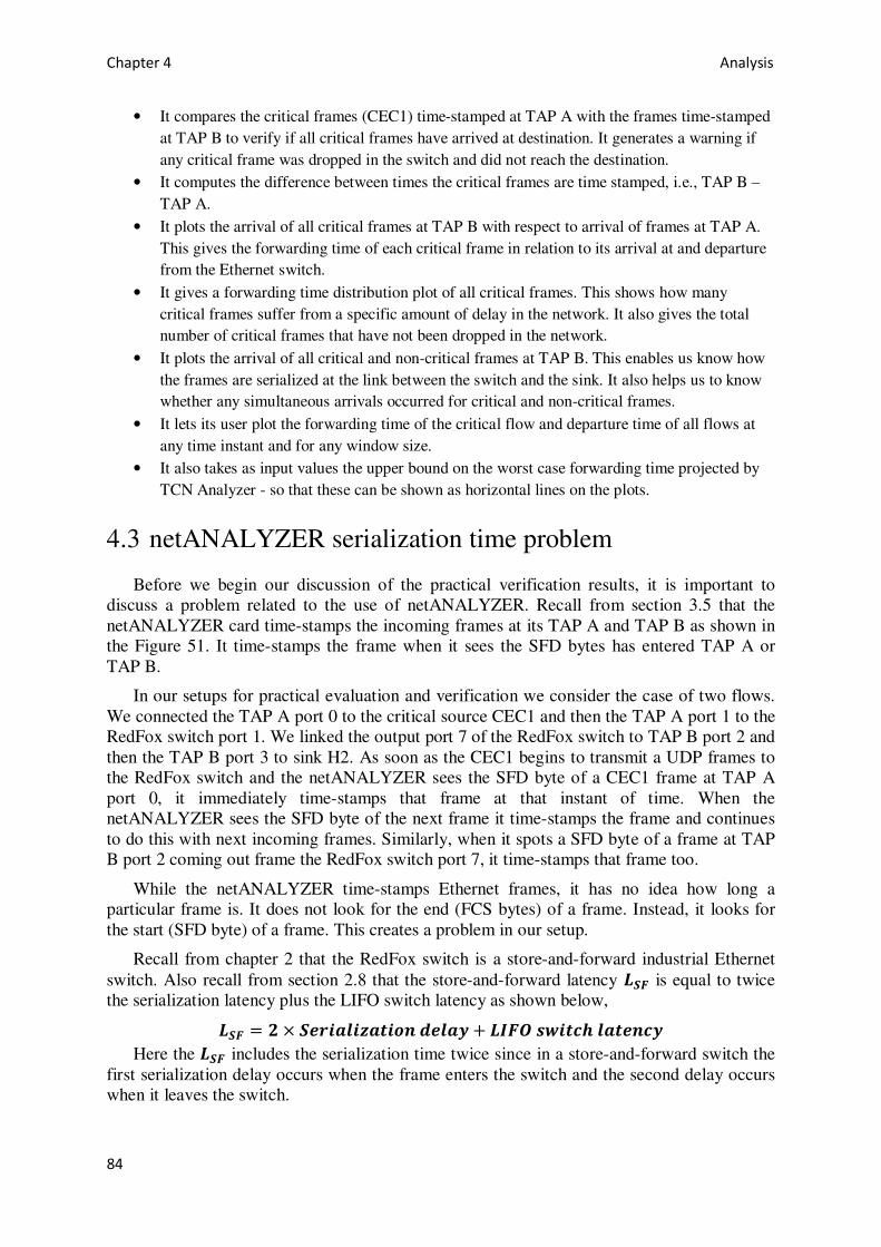
Chapter 4 Analysis
84
• It compares the critical frames (CEC1) time-stamped at TAP A with the frames time-stamped at TAP B to verify if all critical frames have arrived at destination. It generates a warning if any critical frame was dropped in the switch and did not reach the destination.
• It computes the difference between times the critical frames are time stamped, i.e., TAP B – TAP A.
• It plots the arrival of all critical frames at TAP B with respect to arrival of frames at TAP A. This gives the forwarding time of each critical frame in relation to its arrival at and departure from the Ethernet switch.
• It gives a forwarding time distribution plot of all critical frames. This shows how many critical frames suffer from a specific amount of delay in the network. It also gives the total number of critical frames that have not been dropped in the network.
• It plots the arrival of all critical and non-critical frames at TAP B. This enables us know how the frames are serialized at the link between the switch and the sink. It also helps us to know whether any simultaneous arrivals occurred for critical and non-critical frames.
• It lets its user plot the forwarding time of the critical flow and departure time of all flows at any time instant and for any window size.
• It also takes as input values the upper bound on the worst case forwarding time projected by TCN Analyzer - so that these can be shown as horizontal lines on the plots.
4.3 netANALYZER serialization time problem
Before we begin our discussion of the practical verification results, it is important to discuss a problem related to the use of netANALYZER. Recall from section 3.5 that the netANALYZER card time-stamps the incoming frames at its TAP A and TAP B as shown in the Figure 51. It time-stamps the frame when it sees the SFD bytes has entered TAP A or TAP B.
In our setups for practical evaluation and verification we consider the case of two flows. We connected the TAP A port 0 to the critical source CEC1 and then the TAP A port 1 to the RedFox switch port 1. We linked the output port 7 of the RedFox switch to TAP B port 2 and then the TAP B port 3 to sink H2. As soon as the CEC1 begins to transmit a UDP frames to the RedFox switch and the netANALYZER sees the SFD byte of a CEC1 frame at TAP A port 0, it immediately time-stamps that frame at that instant of time. When the netANALYZER sees the SFD byte of the next frame it time-stamps the frame and continues to do this with next incoming frames. Similarly, when it spots a SFD byte of a frame at TAP B port 2 coming out frame the RedFox switch port 7, it time-stamps that frame too.
While the netANALYZER time-stamps Ethernet frames, it has no idea how long a particular frame is. It does not look for the end (FCS bytes) of a frame. Instead, it looks for the start (SFD byte) of a frame. This creates a problem in our setup.
Recall from chapter 2 that the RedFox switch is a store-and-forward industrial Ethernet switch. Also recall from section 2.8 that the store-and-forward latency �� is equal to twice the serialization latency plus the LIFO switch latency as shown below,
�� = * × �� �� ��� ������� + ������ ���������� Here the �� includes the serialization time twice since in a store-and-forward switch the
first serialization delay occurs when the frame enters the switch and the second delay occurs when it leaves the switch.

Chapter 4 Analysis
85
When an Ethernet frame enters TAP A port 0, it is time-stamped there and forwarded to the RedFox switch through TAP A port 1. Since the RedFox switch is of store-and-forward type, the frame stays there for a while until the switch finishes its processing on that frame. After the switch finishes the processing and sends it to the sink, it first enters the netANALYZER TAP B port 2 where it is time-stamped on the arrival of its SFD and from there forwarded to the sink H2 without any delay.
In the setup of netANALYZER we do not take into account the second serialization time of the frame when compute the difference between the time-stamps (TAP B – TAP A) to calculate the forwarding time of the critical frame. We count only first serialization time when the critical frame enters the switch and stays there for a while. However, we do not take into consideration the second serialization time when the stored frame leaves the switch. The first serialization time is included by default since we are using a store-and-forward switch. And because of that the netANALYZER has to wait for the end of frame to enter the switch before it can time-stamp the next frame. The problem arises from the fact that when the switch starts to send the frame to the sink H2, the netANALYZER time-stamps it on the arrival of its SFD byte and not on its last byte of FCS. It does not wait for the complete departure of the frame from the switch before it time-stamps it. This is explained in the Figure 51.
As shown in Figure 51, when the SFD of the red frame enters the netANALYZER it is time-stamped there and forwarded to the switch. The frame then stays in the switch until it is processed and then sent to the sink H2 by the switch via netANALYZER where it is time-stamped again at the arrival of the SFD.

Chapter 4 Analysis
86
Figure 51: Serialization problem in netANALYZER
Because of the above drawback in the use of netANALYZER, we have to manually add one serialization time to the measured forwarding time according to the formula given below. This gives us the actual forwarding time of the critical frame.
�� �� ��� ��� �� =�������� ��
� �!"���� ���+ �����#���� �$(��&)
Here the frame length could be 64 bytes, 514 bytes, 1014 bytes, and 1514 depending upon the measurement. Link bandwidth is 100 Mbps and IFG is 960 ns because of the 100 Mbps link bandwidth.
4.4 Single flow
As described in section 3.3, we began the practical evaluation phase by setting up the network with one critical UDP flow from the UDP source CEC1 to sink H2 through the RedFox switch. After the measurements were recorded into netANALYZER and processed through our Stream Analyzer, we got a series of plots as shown below.
Figure 52 is the forwarding time plot of all critical frames of 64 byte size in this setup of only one UDP flow which is also the critical flow across the RedFox switch. The x-axis

Chapter 4 Analysis
87
shows the time-stamp moment at netANALYZER TAP A whereas the y-axis shows the forwarding time calculated by taking the difference of TAP B and TAP A time-stamps.
The blue horizontal indicates TCN Analyzer estimated maximum forwarding time for this network setup and a single UDP source, while the red horizontal line indicates the compensated value for serialization time of TCN Analyzer predicted maximum forwarding time (blue line). The Stream Analyzer did not add the serialization time to the calculated forwarding time, instead for comparison purposes we subtract one serialization time according to the formula given in section 4.3 from TCN estimation for comparison (this is shown as the horizontal red line).
Figure 52: Forwarding time plot for all critical frames for single flow case. Also shown are the TCN estimated (shown as a blue horizontal line) and the compensated upper bounds (shown as a red
horizontal line).
Figure 53 shows the distribution plot of forwarding times of all critical UDP frames. As shown, there were 63692 critical frames time-stamped and recorded. Most of the frames experienced forwarding time less than 8.0 µs (14.08 µs when compensated for the extra serialization time) delay whereas around 5500 frames suffered 11.44 µs (corresponding to 17.52 µs compensated) delay.

Chapter 4 Analysis
88
Figure 53: Forwarding time distribution plot for all critical UDP frames for the case of one flow Figure 54 shows the forwarding times of critical UDP frames plotted at maximum
forwarding time instant at TAP A. Here we plotted the maximum forwarding time suffered by one or more critical frames. Notice that the arrival of critical frames at TAP A is periodic and we do not see any bursts of frames. This shows that the maximum forwarding time occurred because of the latency in switched Ethernet and not because of the sending node’s unpredictable behavior. Also notice that the measured forwarding time exceeds the compensated TCN estimation. TCN has underestimated the forwarding time and was more optimistic. This may due to the fact (not definitely known) that there was only one flow and TCN Analyzer is meant to deal with more than one flow in the Ethernet network. Nevertheless this very small overestimation will not affect the proposed use of the CAN/Ethernet network.
Figure 54: Forwarding time graph plotted at maximum forwarding time instant for the case of a single flow. Also shown are the TCN estimated (shown as a blue horizontal line) and the compensated upper
bounds (shown as a red horizontal line).
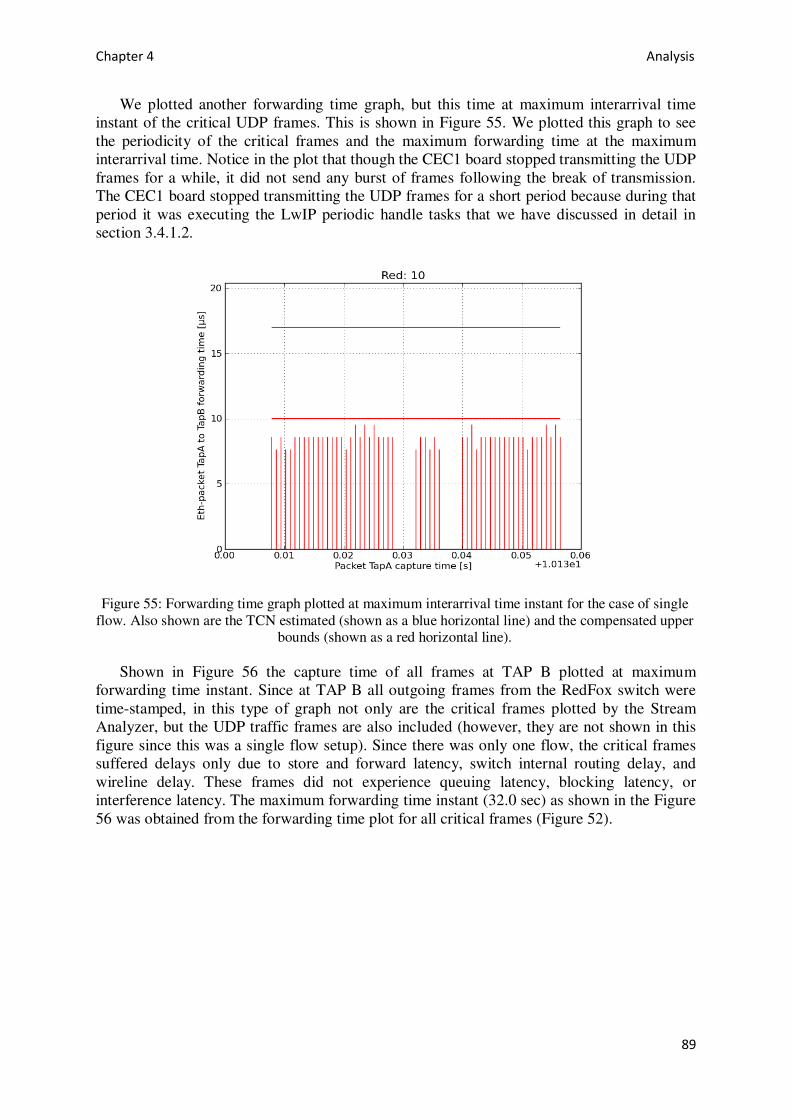
Chapter 4 Analysis
89
We plotted another forwarding time graph, but this time at maximum interarrival time instant of the critical UDP frames. This is shown in Figure 55. We plotted this graph to see the periodicity of the critical frames and the maximum forwarding time at the maximum interarrival time. Notice in the plot that though the CEC1 board stopped transmitting the UDP frames for a while, it did not send any burst of frames following the break of transmission. The CEC1 board stopped transmitting the UDP frames for a short period because during that period it was executing the LwIP periodic handle tasks that we have discussed in detail in section 3.4.1.2.
Figure 55: Forwarding time graph plotted at maximum interarrival time instant for the case of single flow. Also shown are the TCN estimated (shown as a blue horizontal line) and the compensated upper
bounds (shown as a red horizontal line).
Shown in Figure 56 the capture time of all frames at TAP B plotted at maximum forwarding time instant. Since at TAP B all outgoing frames from the RedFox switch were time-stamped, in this type of graph not only are the critical frames plotted by the Stream Analyzer, but the UDP traffic frames are also included (however, they are not shown in this figure since this was a single flow setup). Since there was only one flow, the critical frames suffered delays only due to store and forward latency, switch internal routing delay, and wireline delay. These frames did not experience queuing latency, blocking latency, or interference latency. The maximum forwarding time instant (32.0 sec) as shown in the Figure 56 was obtained from the forwarding time plot for all critical frames (Figure 52).

Chapter 4 Analysis
90
Figure 56: TAP B all frames arrival graph plotted at the maximum forwarding time instant for the case of single flow
Figure 57 shows the graph of all frames sent from the RedFox switch that arrived at sink
H2 via netANALYZER TAP B. The graph is plotted at the maximum interarrival time instant identified from the forwarding time plot for all critical frames (see Figure 52).
Figure 57: TAP B all frames arrival graph plotted at maximum interarrival time instant for the case of single flow
4.5 Seven flows
As described in section 3.3, we carried out the practical evaluation with various number of UDP flows ranging from one to seven including the critical flow. Here we discussed the results and plots obtained from the setup of seven flows each having the Ethernet frame size of 64 bytes including the critical flow. There was one critical UDP flow from CEC1 and six additional UDP traffic flows from CEC2 (via RedFox switch 2) destined to the sink H2 through RedFox switch 1 (see section 3.7.4).
Figure 58 is the forwarding time plot of all critical frames of 64 bytes size in this seven flows setup. The x-axis shows the arrival time of the critical flow CEC1 at netANALYZER TAP A whereas the y-axis shows the forwarding time of the critical flow CEC1 as calculated by taking the difference of TAP B and TAP A time-stamps.
The blue horizontal indicates TCN Analyzer predicted maximum forwarding time and the red horizontal line indicates the serialization compensated value for the TCN Analyzer predicted maximum forwarding time.
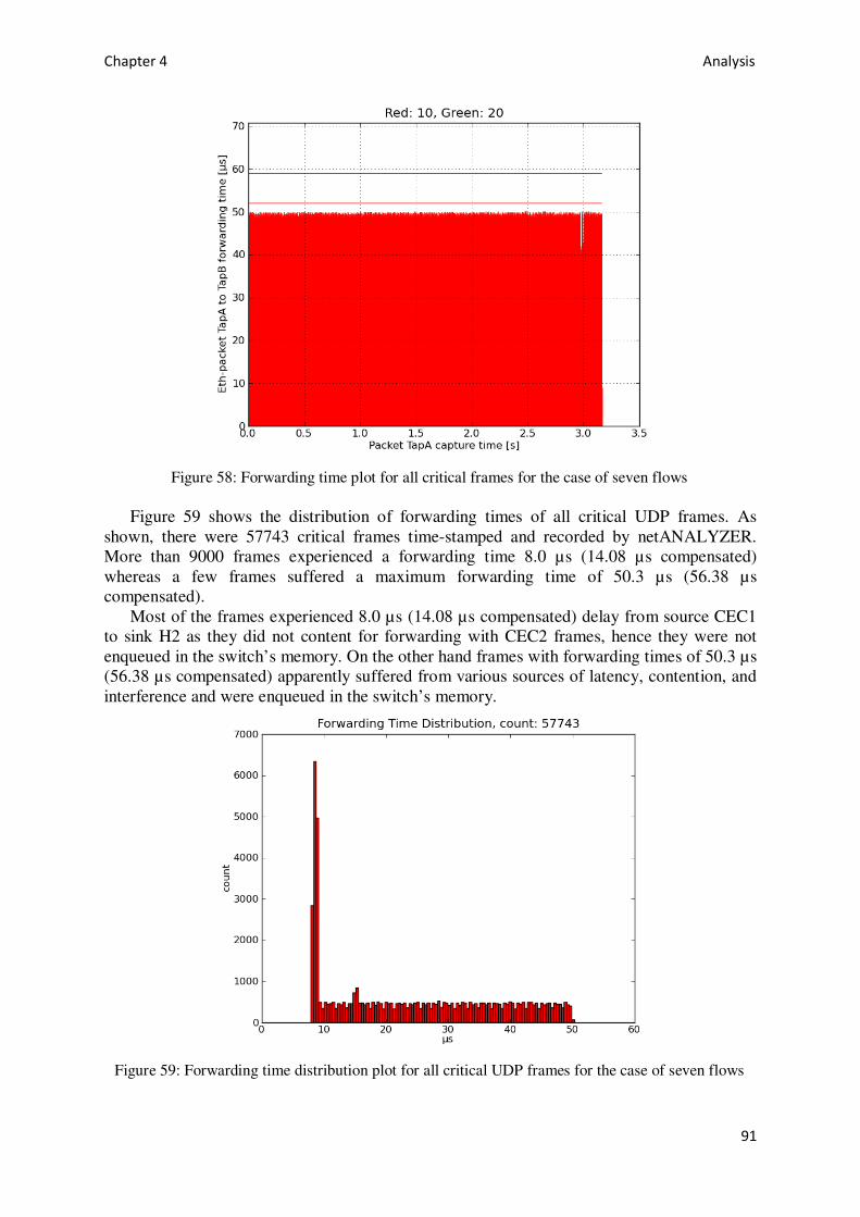
Chapter 4 Analysis
91
Figure 58: Forwarding time plot for all critical frames for the case of seven flows Figure 59 shows the distribution of forwarding times of all critical UDP frames. As
shown, there were 57743 critical frames time-stamped and recorded by netANALYZER. More than 9000 frames experienced a forwarding time 8.0 µs (14.08 µs compensated) whereas a few frames suffered a maximum forwarding time of 50.3 µs (56.38 µs compensated).
Most of the frames experienced 8.0 µs (14.08 µs compensated) delay from source CEC1 to sink H2 as they did not content for forwarding with CEC2 frames, hence they were not enqueued in the switch’s memory. On the other hand frames with forwarding times of 50.3 µs (56.38 µs compensated) apparently suffered from various sources of latency, contention, and interference and were enqueued in the switch’s memory.
Figure 59: Forwarding time distribution plot for all critical UDP frames for the case of seven flows

Chapter 4 Analysis
92
Figure 60 shows the forwarding times of critical CEC1 UDP frames plotted at maximum forwarding time instant. Also shown are the original and compensated TCN estimated worst case forwarding time.
Figure 60: Forwarding time graph plotted at maximum forwarding time instant for the case of seven flows. Also shown are the TCN estimated (shown as a blue horizontal line) and the compensated
upper bounds (shown as a red horizontal line). Notice in Figure 60 the positive slope of adjacent forwarding times. This is because of the
queue of frames that built up inside the RedFox switch 1. All six CEC2 noise frames and the CEC1 critical frame arrived at their respective ports of the RedFox switch 1 concurrently and all of them headed for the same destination sink H2. Moreover, from section 3.3.1 recall that the data rate of the UDP critical source CEC1 and the UDP traffic generator CEC2 were set to slightly different values to increase the probability of simultaneous arrivals. The positive slope indicates that six CEC2 noise frames arrived just before the critical frame CEC1. All the six CEC2 noise frames and the critical frame were enqueued in the switch memory for the amount of time that was equal to the overlapped length of the frames that caused contention in the switch. This phenomenon was explained in detail in section 3.3.1. The six CEC2 frames continued to leave the RedFox switch 1 before the critical frame CEC1 until the last one of the six perfectly arrived at the same time as the critical frame. After that the critical frame began to leave the switch before the six CEC2 frames. As a result the six CEC2 frames were enqueued in the memory behind the CEC1 critical frame that no longer suffered any delay after having arrived at the same time as another frame and we see a minimum forwarding time for the CEC1 critical frame.
Though the negative sloped queue of the six additional frames is not shown in the Figure 60, if we connect the CEC2 traffic to TAP A of netANALYZER and keep the TAP B connection as it was, we will see a negative slope ramp mirrored across the y-axis. An example of a negative slope queue is shown in Figure 72 in appendix A.
The forwarding time graph plotted at maximum interarrival time of the critical UDP frames is shown in Figure 61. Notice here that although the CEC1 board stopped transmitting the UDP frames for a while, it did not send any burst of UDP frames following the break in transmission.
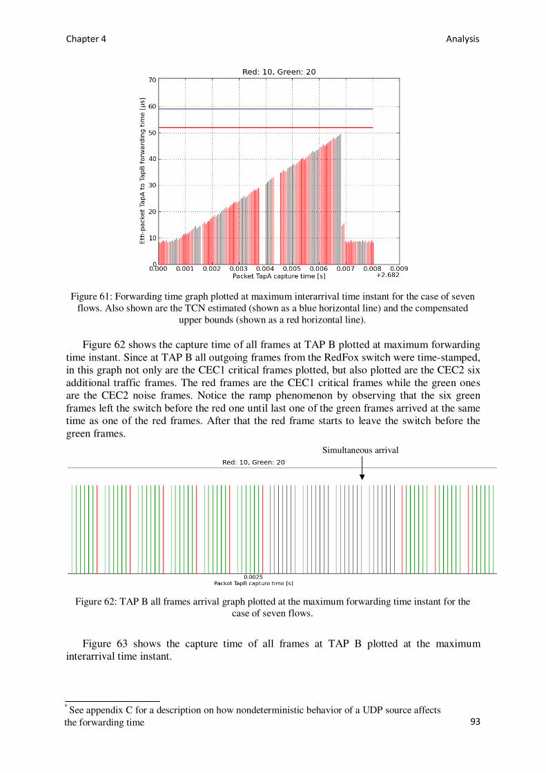
Chapter 4 Analysis
93
Figure 61: Forwarding time graph plotted at maximum interarrival time instant for the case of seven flows. Also shown are the TCN estimated (shown as a blue horizontal line) and the compensated
upper bounds (shown as a red horizontal line). Figure 62 shows the capture time of all frames at TAP B plotted at maximum forwarding
time instant. Since at TAP B all outgoing frames from the RedFox switch were time-stamped, in this graph not only are the CEC1 critical frames plotted, but also plotted are the CEC2 six additional traffic frames. The red frames are the CEC1 critical frames while the green ones are the CEC2 noise frames. Notice the ramp phenomenon by observing that the six green frames left the switch before the red one until last one of the green frames arrived at the same time as one of the red frames. After that the red frame starts to leave the switch before the green frames.
Figure 62: TAP B all frames arrival graph plotted at the maximum forwarding time instant for the case of seven flows.
Figure 63 shows the capture time of all frames at TAP B plotted at the maximum interarrival time instant.
Simultaneous arrival
* See appendix C for a description on how nondeterministic behavior of a UDP source affects the forwarding time
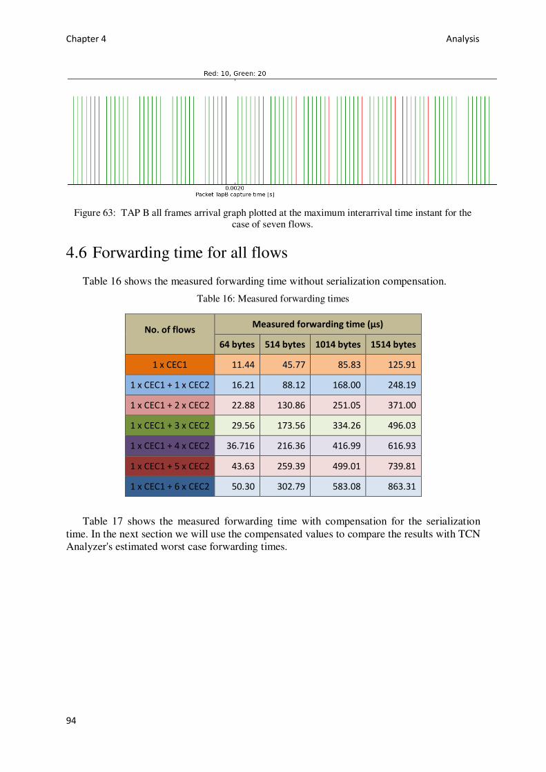
Chapter 4 Analysis
94
Figure 63: TAP B all frames arrival graph plotted at the maximum interarrival time instant for the case of seven flows.
4.6 Forwarding time for all flows
Table 16 shows the measured forwarding time without serialization compensation.
Table 16: Measured forwarding times
No. of flows Measured forwarding time (µs)
64 bytes 514 bytes 1014 bytes 1514 bytes
1 x CEC1 11.44 45.77 85.83 125.91
1 x CEC1 + 1 x CEC2 16.21 88.12 168.00 248.19
1 x CEC1 + 2 x CEC2 22.88 130.86 251.05 371.00
1 x CEC1 + 3 x CEC2 29.56 173.56 334.26 496.03
1 x CEC1 + 4 x CEC2 36.716 216.36 416.99 616.93
1 x CEC1 + 5 x CEC2 43.63 259.39 499.01 739.81
1 x CEC1 + 6 x CEC2 50.30 302.79 583.08 863.31
Table 17 shows the measured forwarding time with compensation for the serialization time. In the next section we will use the compensated values to compare the results with TCN Analyzer's estimated worst case forwarding times.

Chapter 4 Analysis
95
Table 17: Compensated forwarding times
No. of flows Measured forwarding time + Serialization time (µs)
64 bytes 514 bytes 1014 bytes 1514 bytes
1 x CEC1 17.52 87.85 167.91 247.99
1 x CEC1 + 1 x CEC2 22.29 130.20 250.08 370.27
1 x CEC1 + 2 x CEC2 28.96 172.94 333.13 493.08
1 x CEC1 + 3 x CEC2 35.64 215.64 416.34 618.11
1 x CEC1 + 4 x CEC2 42.80 258.44 499.07 739.01
1 x CEC1 + 5 x CEC2 49.71 301.47 581.09 861.89
1 x CEC1 + 6 x CEC2 56.38 344.87 665.16 985.39
Figure 64 shows a bar graph of the measured forwarding time with compensation for the
serialization time.
Figure 64: Bar graph for (compensated) measured forwarding times
0
200
400
600
800
1000
1200
1 2 3 4 5 6 7
Fo
rwa
rdin
g t
ime
(μ
s)
No. of flows
Measured Forwarding Time
64 bytes
514 bytes
1014 bytes
1514 bytes

Chapter 4 Analysis
96
4.7 Comparison: Theoretical vs. Practical
In this section we present TCN Analyzer’s estimated maximum forwarding time and the measured forwarding time. Table 18 compares the TCN Analyzer estimated worst case forwarding time and the (compensated) measured forwarding time for the CEC1 critical UDP flow having the Ethernet frame size of 64 bytes. Except the single flow case, the remaining cases suggest that TCN Analyzer estimates are reasonable and that no frame will suffer delay greater than the estimated delay.
Table 18: Comparison of TCN Analyzer projected and (compensated) measured forwarding times of 64 bytes frame size flows.
No. of Flows Forwarding time (64 bytes)
Measured (µs) TCN (µs)
1 x CEC1 17.52 17
1 x CEC1 + 1 x CEC2 22.29 24
1 x CEC1 + 2 x CEC2 28.96 31
1 x CEC1 + 3 x CEC2 35.64 38
1 x CEC1 + 4 x CEC2 42.80 45
1 x CEC1 + 5 x CEC2 49.71 52
1 x CEC1 + 6 x CEC2 56.38 59
Figure 65 shows a bar graph that compares the TCN Analyzer estimates and the
(compensated) measured forwarding time for the CEC1 critical UDP flow having the Ethernet frames of size 64 bytes.
Figure 65: Bar graph comparing TCN Analyzer projected and measured forwarding times of 64 bytes frame size flows.
0
10
20
30
40
50
60
70
1 2 3 4 5 6 7
Fo
rwa
rdin
g t
ime
(μs)
No. of flows
Measured vs. TCN forwarding times (64 bytes)
Measured
TCN
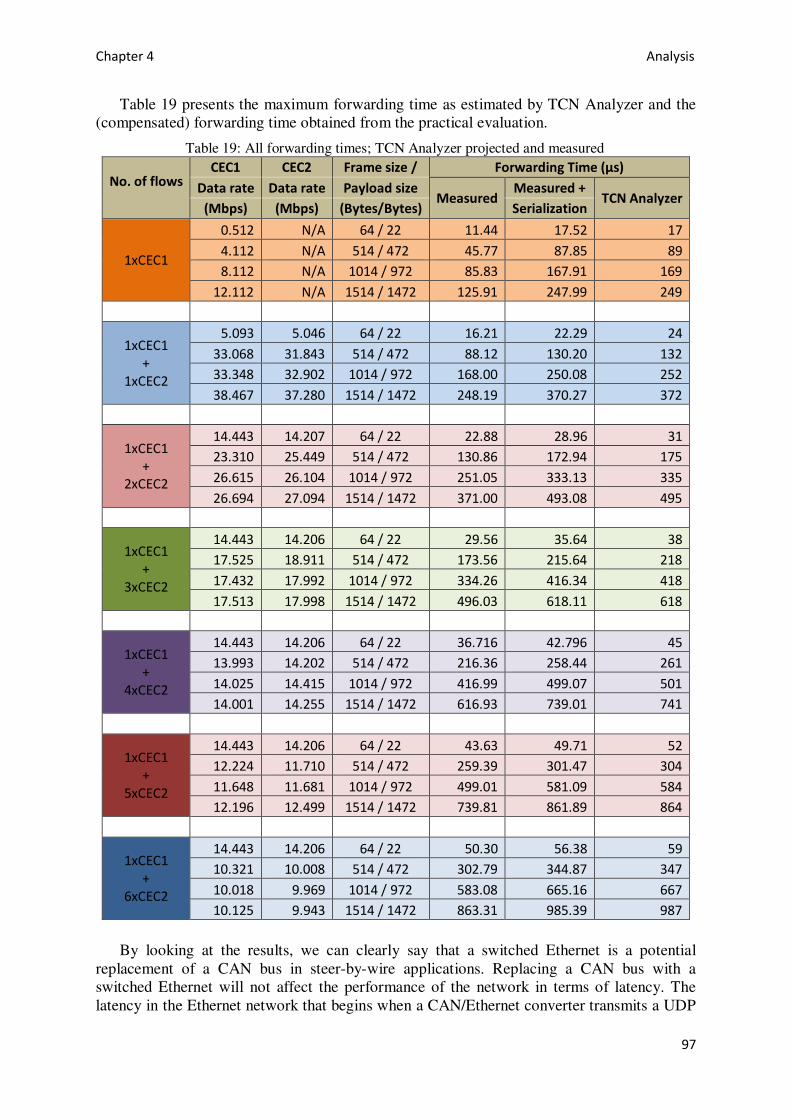
Chapter 4 Analysis
97
Table 19 presents the maximum forwarding time as estimated by TCN Analyzer and the (compensated) forwarding time obtained from the practical evaluation.
Table 19: All forwarding times; TCN Analyzer projected and measured
No. of flows CEC1 CEC2 Frame size / Forwarding Time (μs)
Data rate Data rate Payload size Measured
Measured + TCN Analyzer
(Mbps) (Mbps) (Bytes/Bytes) Serialization
1xCEC1
0.512 N/A 64 / 22 11.44 17.52 17
4.112 N/A 514 / 472 45.77 87.85 89
8.112 N/A 1014 / 972 85.83 167.91 169
12.112 N/A 1514 / 1472 125.91 247.99 249
1xCEC1
+
1xCEC2
5.093 5.046 64 / 22 16.21 22.29 24
33.068 31.843 514 / 472 88.12 130.20 132
33.348 32.902 1014 / 972 168.00 250.08 252
38.467 37.280 1514 / 1472 248.19 370.27 372
1xCEC1
+
2xCEC2
14.443 14.207 64 / 22 22.88 28.96 31
23.310 25.449 514 / 472 130.86 172.94 175
26.615 26.104 1014 / 972 251.05 333.13 335
26.694 27.094 1514 / 1472 371.00 493.08 495
1xCEC1
+
3xCEC2
14.443 14.206 64 / 22 29.56 35.64 38
17.525 18.911 514 / 472 173.56 215.64 218
17.432 17.992 1014 / 972 334.26 416.34 418
17.513 17.998 1514 / 1472 496.03 618.11 618
1xCEC1
+
4xCEC2
14.443 14.206 64 / 22 36.716 42.796 45
13.993 14.202 514 / 472 216.36 258.44 261
14.025 14.415 1014 / 972 416.99 499.07 501
14.001 14.255 1514 / 1472 616.93 739.01 741
1xCEC1
+
5xCEC2
14.443 14.206 64 / 22 43.63 49.71 52
12.224 11.710 514 / 472 259.39 301.47 304
11.648 11.681 1014 / 972 499.01 581.09 584
12.196 12.499 1514 / 1472 739.81 861.89 864
1xCEC1
+
6xCEC2
14.443 14.206 64 / 22 50.30 56.38 59
10.321 10.008 514 / 472 302.79 344.87 347
10.018 9.969 1014 / 972 583.08 665.16 667
10.125 9.943 1514 / 1472 863.31 985.39 987
By looking at the results, we can clearly say that a switched Ethernet is a potential
replacement of a CAN bus in steer-by-wire applications. Replacing a CAN bus with a switched Ethernet will not affect the performance of the network in terms of latency. The latency in the Ethernet network that begins when a CAN/Ethernet converter transmits a UDP

Chapter 4 Analysis
98
frame in a 64 bytes Ethernet frame carrying a CAN message and ends when the receiving CAN/Ethernet converter collects that message is much less than the maximum allowable latency of 1ms. Furthermore notice that flows with frame sizes other than 64 bytes will not suffer delays greater than 1ms according to TCN Analyzer and also confirmed by measurements. Therefore we can say that we can transmit data of large payload sizes along with CAN messages carrying frames without worrying about delays in the Ethernet network.
While the latency of the switched Ethernet will not affect the performance of the CAN nodes, it must be noted that the guarantee that TCN Analyzer gives to the CAN/Ethernet designer is based on the assumption that the sum of the ingress data rates is less than or equal to egress link rate. Additionally, we are not taking into consideration the CAN bus speed and the CAN/Ethernet conversion time when calculating the latency in a switched Ethernet.
4.8 CAN/Ethernet conversion time & end-to-end latency
Section 3.8 described the setup used to calculate the time taken by the CAN/Ethernet converter to encapsulate a CAN message into a UDP datagram and emit it as an Ethernet frame and vice versa. Using this setup and taking the difference of netANALYZER TAP A time-stamp and TAP B time-stamp gives us the delays shown in Figure 66. Ethernet serialization delay occurs when Comm Operator Pal generates Ethernet frames of 64 byte size (we used 64 bytes frame size because one complete CAN message can reside in the 22 byte UDP payload field of this size frame). Ethernet to CAN conversion delay occurs inside the CAN/Ethernet converter, CAN serialization delay occurs when the first CAN/Ethernet converter transmits a CAN message to another CAN/Ethernet converter. Finally the last Ethernet serialization delay occurs when the second CAN/Ethernet converter sends Ethernet frame to the sink H2. This last serialization is missed by the netANALYZER in time-stamping the frame at its TAP B (see section 4.3).
Figure 66: Delays in the CAN/Ethernet conversion time measurement setup. (Delays shown as boxes are not drawn to scale)
Table 20 shows the TAP A and TAP B time-stamps values measured by the
netANALYZER in the setup. We have taken the average of five TAB B – TAP A values to get the sum of delays as described above.

Chapter 4 Analysis
99
Table 20: TAP A and TAP B time-stamps Time-stamps (sec)
TAP A TAP B TAP B - TAP A
1.63864463 1.63884149 0.00019686
2.28365714 2.28385424 0.00019710
2.35180653 2.35200347 0.00019694
2.42198793 2.42218469 0.00019676
2.52304309 2.52323991 0.00019682
Average TAP B - Tap A 0.000196896 sec
To obtain the Ethernet to CAN conversion delay and CAN to Ethernet conversion delay values, we have to subtract one Ethernet serialization delay and one CAN serialization delay from the averaged TAP B -TAP A value calculated in the above table.
We know from section 4.3 that the serialization time is equal to,
Serializationtime =Framelength
Linkbandwidth+ Interframegap(IFG)
Here, Framelength = 64bytes
Linkbandwidth = 100Mbps Interframegap = 960ns
Therefore, EtherentSerializationtime = 6.08us
Similarly to calculate the CAN serialization time we use the same equation with,
Framelength = 19bytes(approximate) Linkbandwidth = 1Mbps
Interframegap = 3μs(InterFrameSpace)
Therefore, CANSerializationtime = 155μs(approx)
Using the above calculated total delay, CAN serialization delay, and Ethernet serialization delay, we can calculate the CAN/Ethernet conversion delay as follows,
2xCAN/Ethernetconversiondelay = 196.896 − 155 − 6.08
*h��i/jklmnomkpqormnstqoumvwx = /2. 0-yμs
Thus the CAN/Ethernet conversion comes out to be around 18 µs. We will use this delay and the maximum forwarding time projected by TCN Analyzer to calculate the end-to-end delay in the CAN/Ethernet network.
Figure 67 shows the delays that occur in our CAN/Ethernet network. The delay includes the forwarding time that is projected by TCN Analyzer and the latency that will be introduced by the CAN/Ethernet network if we replace the CAN bus with Ethernet. The left most CAN serialization is the normal CAN serialization that occur in the CAN bus, i.e. it occurs when a CAN node sends a message to another CAN node over the CAN bus. Since our CAN/Ethernet network did not introduce this delay, we will not include it in the end-to-end latency calculation.

Chapter 4 Analysis
100
Figure 67: End-to-End latency in CAN/Ethernet network. (Delays shown as boxes are not drawn to scale)
To calculate the end-to-end latency we need to add the CAN to Ethernet conversion
delay, TCN estimated forwarding time, Ethernet serialization delay, Ethernet to CAN conversion delay, and the CAN serialization delay. Table 21 shows the worst case end-to-end latency in our CAN/Ethernet network. Column 1 shows the number of CAN/Ethernet converters that are linked to the switch including source and destination. Here the worst case is considered when we have one to seven sources sending UDP messages simultaneously to the same sink. TCN Analyzer forwarding times are those that are estimated by it for a 64 byte Ethernet frame size. The CAN serialization time 1240 µs, 620 µs, and 155 µs are calculated for 125 kbps bus, 250 kbps bus and 1 Mbps bus data rates respectively.
Table 21: Worst case end-to-end latency in CAN/Ethernet network
No. of
CAN/Ethernet
converters
2xCAN/Ethernet TCN Analyzer CAN End-to-End
conversion delay
(µs)
Forwarding time
(µs)
Serialization
time (µs) latency (µs)
2 35.816 17
1240 1292.816
620 672.816
155 207.816
3 35.816 24
1240 1299.816
620 679.816
155 214.816
4 35.816 31
1240 1306.816
620 686.816
155 221.816
5 35.816 38
1240 1313.816
620 693.816
155 228.816
6 35.816 45
1240 1320.816
620 700.816
155 235.816
7 35.816 52
1240 1327.816
620 707.816
155 242.816
8 35.816 59
1240 1334.816
620 714.816
155 249.816

Chapter 4 Analysis
101
One can notice in Table 21 that the end-to-end latency is primarily due to the CAN serialization time. After calculating the CAN/Ethernet end-to-end latency, we now observe a barrier in the way of replacing CAN bus with Ethernet with CAN/Ethernet converters. The shortcoming in terms of latency in our CAN/Ethernet network is the additional CAN serialization delay. This causes the end-to-end latency to exceed the CAN applications’ allowed latency of 1ms. However, if we ensure that the CAN bus operates at 1 Mbps, then
we can limit the CAN serialization time to 155 µs -- then in all cases the total end-to-end
latency is well under 1 ms.
4.9 Bandwidth utilization
In this section we analyze the bandwidth utilization in our proposed CAN/Ethernet network with the same number of sources and sink and the same RedFox switch. As described before, the standard CAN bus speed varies from 10 kbps to 1 Mbps. The most common bus speeds are 125 kbps, 250 kbps, and 1 Mbps. Whereas the Ethernet link rate that we used in our project is 100 Mbps.
Table 22 shows the maximum bandwidth utilization in our CAN/Ethernet converter with 1Mbps CAN bus speed. Here the first column indicates the number of CAN/Ethernet converters connected to the switch. We have taken the worst case scenario in each bandwidth utilization value. We assume that the CAN/Ethernet converter is receiving CAN message from its CAN node(s) at the full bus speed of 1 Mbps. This implies that each converter is receiving a message at 160 µs intervals. Encapsulation of this CAN message into a UDP frame requires 22 bytes UDP payload size leading to a 64 bytes size Ethernet frame. Continuously transmitting this message with an interarrival time of 160 µs results in an Ethernet data rate of 3.2 Mbps including the IFG.
Now if seven out of eight CAN/Ethernet converters transmit at 3.2 Mbps to the eighth CAN/Ethernet converter via RedFox switch, the receiving CAN/Ethernet converter will be receiving Ethernet frames at 22.4 Mbps which is 22.4% of 100 Mbps bandwidth. This comes from the fact that across the switch the egress data rate is equal to the sum of the ingress data rates which are governed by the CAN bus speed in this case.
Here we assume that the receiving CAN/Ethernet converter has enough buffers to handle all the CAN/Ethernet conversions with maximum data rates. Since at the receiving CAN/Ethernet converter the ingress Ethernet data rate (3.2 Mbps to 22.4 Mbps) is much greater than the egress CAN data rate (1 Mbps), therefore we need some sort of buffering inside the CAN/Ethernet converter to avoid loss of messages. Depending on the maximum bound on end-to-end delay, we can calculate the number of bytes of buffering that is needed in the converter.
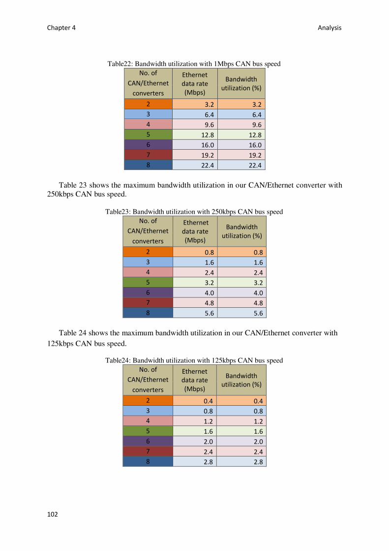
Chapter 4 Analysis
102
Table22: Bandwidth utilization with 1Mbps CAN bus speed No. of
CAN/Ethernet
converters
Ethernet
data rate
(Mbps)
Bandwidth
utilization (%)
2 3.2 3.2
3 6.4 6.4
4 9.6 9.6
5 12.8 12.8
6 16.0 16.0
7 19.2 19.2
8 22.4 22.4
Table 23 shows the maximum bandwidth utilization in our CAN/Ethernet converter with
250kbps CAN bus speed.
Table23: Bandwidth utilization with 250kbps CAN bus speed No. of
CAN/Ethernet
converters
Ethernet
data rate
(Mbps)
Bandwidth
utilization (%)
2 0.8 0.8
3 1.6 1.6
4 2.4 2.4
5 3.2 3.2
6 4.0 4.0
7 4.8 4.8
8 5.6 5.6
Table 24 shows the maximum bandwidth utilization in our CAN/Ethernet converter with 125kbps CAN bus speed.
Table24: Bandwidth utilization with 125kbps CAN bus speed No. of
CAN/Ethernet
converters
Ethernet
data rate
(Mbps)
Bandwidth
utilization (%)
2 0.4 0.4
3 0.8 0.8
4 1.2 1.2
5 1.6 1.6
6 2.0 2.0
7 2.4 2.4
8 2.8 2.8

Chapter 4 Analysis
103
4.10 Validation results
Although the end-to-end latency exceeded the allowed latency of 1ms of CPAC Systems’ CAN applications, we tested and tried to validate our proposed CAN/Ethernet network on the CPAC Systems’ test rigs as described in section 3.9. In table 25 we present the results of those tests. Note that all of the tests were passed even with the shortcoming of CAN serialization delay that occurs in our CAN/Ethernet network.
Table 25: CPAC Systems rigs tests results
Test Version Rig Result
4.11 Single IPS, one station (Figure 47)
Procedure: Start engine, move lever forward/reverse.
Acceptance: Engine is started. Forward gear is set when moving lever
to forward, reverse gear is set when moving lever to reverse.
EVC 1219 Pimp OK
Procedure: Auto configuration performed.
Acceptance: No faults present in the system EVC 1219 Pimp OK
Twin IPS, three stations (Figure 49)
Procedure: Auto configuration performed.
Acceptance: No faults present in the system. Make sure joystick and
steering wheel are configured.
EVC 1219 Pimp OK
Procedure: Start engine.
Acceptance: Engines are started. EVC 1219 Pimp OK
Procedure: Activate joystick.
Acceptance: Joystick activated and controls the movement of the
drives.
EVC 1219 Pimp OK
Procedure: Turn Steering wheel.
Acceptance: Drives moves when steering wheel is turned. EVC 1219 Pimp OK
Procedure: Start engine. Move levers, gear forward and reverse.
Acceptance: Engines started. Both forward and reverse gear can be
set.
EVC 1219 Pimp OK
Procedure: Calibration of joystick.
Acceptance: Joystick is calibrated accurately. EVC 1219 Pimp OK
Procedure: Fault injection, disconnected SUS Can communication.
Acceptance: Diagnostic code present in the system, indicating that
SUS com has been disconnected.
EVC 1219 Pimp OK

5 Conclusions and Future Work In this final chapter we summarize the results of the thesis project. We look at the goals
outlined in the proposal and review what has been carried out. We will examine how we proceeded through the different phases of the project and discuss if we have achieved our goals. To do so, we will look at the outcomes of every phase of this project. We conclude by trying to give a concrete answer to the basic question underlying this research. Moreover, we provide suggestions to those who want to investigate this matter further.
5.1 Summary
The purpose of this thesis project was to evaluate the possibility of replacing the CAN bus, because of its limited data rate, bandwidth dependent bus length, and drawbacks in network topology, with an Ethernet using COTS hardware (specifically Ethernet switches). CAN is meant to be a high-integrity communication bus and was designed to be deterministic and cost-effective. On the other hand Ethernet, albeit with the advent of Ethernet switch has minimized its non-deterministic behavior, but it is commonly still considered unreliable for time critical applications.
Using a modeling tool, in this case TCN Analyzer, makes it possible to estimate an upper bound on the forwarding time of a frame in an Ethernet network, thereby allowing us to evaluate if Ethernet can be used with for specific time-critical applications. In this thesis project we sought to answer the following question:
How long does it take for a critical message to traverse the
Ethernet network and arrive at its destination? The research has been carried out in three phases, theoretical evaluation phase, practical
verification phase, and validation phase.
In the theoretical phase we studied the IEEE 802.3 specifications in detail, as a technology to support protocols typical of the automotive industry. This implies transferring data packets of a small size. We analyzed the layered architecture of the network and the functions implemented on each layer. We investigated the reasons behind the latency in a switched Ethernet, and modeled various Ethernet networks, based on the CPAC Systems’ architectural requirements. Modeling was performed by means of TCN Analyzer, a very new tool to model an Ethernet network in order to predict its real-time performance.
TCN Analyzer (or, more precisely, the algorithm implemented within the tool) was a key element motivating this work. The tool makes it possible to assess the maximum latency of an Ethernet frame across the network, and whether there is a risk of messages being lost because of excessive data traffic. This is extremely important information:
• It represents the maximum possible delay in the transmission of a message of critical importance.
• It indicates whether there is a risk that a message be lost in a certain traffic condition. • Because of the aforesaid, it is a guideline in dimensioning the network itself.
By looking at the results yielded by the TCN Analyzer, we could assess that the time taken by a critical message to traverse the Ethernet network was much shorter than 1 ms, the maximum acceptable latency according to the CPAC Systems’ architectural requirements.

Chapter 5 Conclusion and Future Work
106
The frames will not suffer delays greater than 1 ms irrespective of their length. That is, the size of the payload does not cause the transmission delay to rise above the acceptable limit.
A verification of the results provided by the TCN analyzer was performed experimentally. To do so, we built the Ethernet network previously modeled and tried to identify the boundary of the model reliability by stress testing the network. However, we did not find any significant deviation from the estimated maximum latency values.
After the promising results from the theoretical phase and from the verification phase, we continued our validation of the solution by means of a direct system test. We installed the CAN/Ethernet network on the test rigs of CPAC Systems and performed tests according to the standard procedure followed by the company to test the CAN network, including the bus and nodes, on a functional level. The test results were successful and the CAN/Ethernet network did not cause any faults in the system.
5.2 Learning
While carrying out this thesis project, we gained insights about many topics. We learned about the architecture, characteristics, and advantages & disadvantages of both CAN and Ethernet networks. We learned in detail how to port a TCP/IP protocol stack to an ARM based embedded system. We learned how to model networks with the TCN Analyzer.
Generally speaking, all of the phases contributed to an extensive learning about the technologically relevant topics. The fact that the vehicle industry is simultaneously carrying out a number of projects related to Ethernet reassures us that this knowledge is highly relevant.
5.3 Conclusions
We believe that the analysis of the work described in chapter 4, in terms of both methodology and implementation, constitutes a valid foundation for the following statements.
• Within the context represented by CPAC Systems’ application segment, Ethernet is a potential replacement of CAN bus in steer-by-wire applications. If the CAN bus is completely replaced with the Ethernet, the performance of the network will not be affected – on the contrary, as a result of the replacement, the bandwidth may be significantly increased.
• Ethernet can be a suitable solution when it comes to functions of increasing complexity, more differentiated products and/or implementing systems with higher throughput requirements. For instance, data traffic of critical relevance such as alarm messages can be transferred on the same network together with data traffic of non-critical relevance yet requiring high data rate, e.g. a video data flow. The model makes it possible to ensure that no critical data packet will be dropped or delayed beyond the acceptable limit(s).
5.4 Future Work
Notwithstanding the very positive result, the relationship between the complexity of the overall realization – from modeling to final validation – seems to suggest that there may be several possibilities for improvement. In fact, we thought about several areas for improvement during the project. As a reasonable compromise between theory and practical needs, the work plan was focused on producing a concrete result by covering the complete

Chapter 5 Conclusion and Future Work
107
scope from analysis to validation, rather than improving every specific detail. Now we can spend some time to think about those details.
In the current version of the TCN Analyzer modeling, the size of the critical frame is equal to the size of the UDP frames that are being transmitted simultaneously. We can improve the theoretical framework by modeling the UDP flows to account for frames of different sizes being transferred simultaneously across the network. We can verify the results by carrying out an experimental validation, as we did before. This would give us information about how the switch manages the allocation of its shared memory to frames of different sizes and how this affects the forwarding time. Needless to say, this would also tell us whether the modeling of the switch has been done properly in relation to such a use case.
We can improve the modeling capabilities of the TCN Analyzer by including models of those components which were used for the practical evaluation, but not in the theoretical phase. These components are the CAN/Ethernet converter, the CAN nodes, and the CAN bus itself. By doing so, we would take into consideration the CAN/Ethernet conversion time, the CAN serialization delay, and the CSMA/CD nature of the CAN bus. This could be interesting if the application case is the extension of the CAN network by Ethernet, rather than a complete replacement. In fact, this would give a CAN/Ethernet network architect the possibility to estimate an upper bound on application end-to-end latency. The architect could design a hybrid CAN/Ethernet network according to the real time requirements of each application.
Recalling from section 4.5 that when calculating the bandwidth utilization, we discussed the worst case scenario – i.e. seven CAN/Ethernet converters sending UDP frames via a switch to a single CAN/Ethernet receiver. In that case we assumed the number of buffers in the CAN/Ethernet converter would be sufficient to avoid loss of messages. Actually, the number of buffers required by the CAN/Ethernet converter could be calculated as a function of the number of CAN nodes, number of message flows, and a few additional parameters. This design could also be modeled and simulated in the TCN analyzer.
Also recall from section 4.2.2 we discussed the behavior of the board when it stopped transmitting frames for a short period of time. This was due to the LwIP periodic tasks that the main application called periodically. There will be a need in future to avoid this by modifying the main application to call the periodic tasks without affecting the transmission of frames.
If we now look at how to optimize the exploitation of the possibilities offered by the Ethernet in the context described within this work, we can find a couple of interesting points deserving a technical discussion.
Recall from section 2.2 that CAN is a CSMA/CD bus which includes a prioritization mechanism. When two nodes try to transmit at once, one of the two prevails over the other and transmits its message over the bus. . The node which has lost this arbitration has to re-attempt transmitting its message. However, a node connected to a CAN/Ethernet converter (assuming it is the only device connected to the CAN port of the converter) does not have to deal with bus access arbitration, hence the message sent to the converter is forwarded immediately to the switch where it is buffered as necessary until it can be set on the proper outgoing port. This suggests that there is room for improvement on the node application level to exploit the properties of a switched Ethernet.
One way to avoid the adverse affect due to the CAN’s additional serialization time on the end-to-end larceny in the CAN/Ethernet network is by installing one CAN/Ethernet converter at only one CAN node (such as at ECU) instead of two. At the other end of the network (such

Chapter 5 Conclusion and Future Work
108
as HCU) we can avoid the second CAN/Ethernet converter by changing the node interface (such as HCU interface) from CAN to Ethernet. In this way we avoid the CAN’s additional serialization problem and hence its adverse affect on the end-to-end latency. This will bring the end-to-end latency well below 1ms of maximum allowable latency in CPAC Systems’ CAN applications for the case of 125kbps CAN bus speed.
If we think about the cost of the hardware, then an obvious improvement is the
replacement of the CAN transceiver in each node with an Ethernet interface, with no need for external converters. Thanks to the layered architecture of both CAN and Ethernet, this could be done with virtually no impact in terms of application code changes. An advantage of such an approach would be that the CAN message serialization time would no longer contribute significantly to the message transfer delay. The benefit, in terms of reduced delay and increase aggregate data rates, is rather evident.

Bibliography and references
[1] Microchip Technology Inc. PIC18F87J60. Retrieved June 11, 2011, from http://www.microchip.com/wwwproducts/Devices.aspx?dDocName=en026442
[2] IEEE 802.3-2008: Standard for Information technology-Specific requirements - Part 3: Carrier Sense Multiple Access with Collision Detection (CSMA/CD) Access Method and Physical Layer Specifications.
[3] J. Axelson. "Embedded Ethernet and Internet complete." 16-18. Madison: Lakeview Research LLC, 2003.
[4] IEEE 802.3ba-2010: Standard for Information technology-Specific requirements – Part 3: Carrier Sense Multiple Access with Collision Detection (CSMA/CD) Access Method and Physical Layer Specifications. Amendment 4: Media Access Control Parameters, Physical Layers and Management Parameters for 40 Gbps and 100 Gbps Operation.
[5] ARINC 664, Aircraft Data Network, Part 7: Deterministic Networks, 2003.
[6] “Road Vehicles – Interchange of Digital Information – Controller Area Network (CAN) for High Speed Communication”, ISO DIS 11898 (February 1992).
[7] P. Pedreiras, R. Leite, and L. Almeida. “Characterizing the real-time behavior of prioritized switched Ethernet” [C] Proceedings of 2nd International Workshop on
Real-Time LANs in the Internet Age. Oporto,Portugal,2003.
[8] J. Loeser and H. Haertig. “Low-latency hard real-time communication over switched Ethernet”[C] Proc. of the 16th Euromicro Conference on Real-Time Systems, Catania, Sicily, 2004-07.
[9] J. V. Carbo, J. T. Massanet, and E. H. Orallo. (2010). Analysis of Switched Ethernet for Real-Time Transmission, Factory Automation, Javier Silvestre-Blanes (Ed.), ISBN: 978-953-307-024-7, InTech, Available from: http://www.intechopen.com/articles/show/title/analysis-of-switched-ethernet-for-real-time-transmission
[10] Wikipedia. List of World's Longest Ships. http://en.wikipedia.org/wiki/List_of_world's_longest_ships (accessed 06 11, 2011).
[11] ISO/IEC Standard 7498-1, Information Technology —Open System Interconnection — Basic Reference Model: The Basic Model, 1994.
[12] Bosch. (1991), CAN Specification version 2.0, Stuttgart: Robert Bosch GmbH.
[13] CAN-in-Automation, CANopen, CAL-based Communication Profile for Industrial Systems, CiA DS-301, Version 4.0, June 16 1999.

Bibliography and references
110
[14] DeviceNet Technology Overview, ODVA. DeviceNet Technology Overview. http://www.odva.org/Portals/0/Library/Publications_Numbered/PUB00026R1.pdf (accessed 06 11, 2011).
[15] "Serial Control and Communications Heavy Duty Vehicle Network - Top Level Document", J1939 Revision Number: A, 14 April 2011. http://standards.sae.org/j1939_201104/
[16] Copley Controls Corp. CANopen Network CAN bus Cabling Guide. http://www.copleycontrols.com/motion/pdf/CAN-Bus.pdf (accessed 06 11, 2011).
[17] Softing AG. CAN bus Data-Rate/Bus-Length Ratio. http://www.softing.com/home/en/industrial-automation/products/can-bus/more-can-bus/bit-timing/data-rate-bus-length.php?navanchor=3010537 (accessed 06 11, 2011).
[18] OSEK/VDX. Operating System. February 17, 2005. http://portal.osek-vdx.org/files/pdf/specs/os223.pdf (accessed June 12, 2011).
[19] D-I-X, "The Ethernet - A Local Area Network: Data Link Layer and Physical Layer Specifications", Digital, Intel, and Xerox, 1982.
[20] IEEE Standard 802.3x, Specification for 802.3 Full Duplex Operation, 1997 (now published as part of [IEEE98e]].
[21] R. Braden “Requirements for Internet Hosts-Communication Layers”, RFC Editor, ISSN 2070-1721, .RFC 1122, October 1989.
[22] J. Postel., Internet Protocol”, RFC Editor, ISSN 2070-1721, RFC 791, “September 1981.
[23] D. C. Plummer. “Ethernet Address Resolution Protocol: Or converting network protocol addresses to 48 bit Ethernet address for transmission on Ethernet hardware”, RFC826, November 1982.
[24] J. Postel. “Internet Control Message Protocol”, RFC Editor, ISSN 2070-1721, RFC 792, September 1981.
[25] R. Droms. “Dynamic Host Configuration Protocol”, RFC Editor, ISSN 2070-1721, RFC 2131, March 1997.
[26] J. Postel. “Transmission Control Protocol”, RFC Editor, ISSN 2070-1721, RFC 793, September 1981.
[27] J. Postel. “User Datagram Protocol”, RFC Editor, ISSN 2070-1721, RFC 768, August 1980.
[28] A. Dunkels. The uIP Embedded TCP/IP Stack, Stockholm, Swedish Institute of Computer Science, 2006.

Bibliography and references
111
[29] A. Dunkels. LwIP - A Lightweight TCP/IP stack. October 2002. http://savannah.nongnu.org/projects/lwip/ (accessed June 30, 2011).
[30] G. Lancaster., uC/IP - TCP/IP for microcontrollers. January 09, 2002. http://ucip.sourceforge.net/ (accessed June 12, 2011).
[31] InterNiche Technologies, Inc. NicheStack IPv4 - The Standard For Embedded
TCP/IP. 2005. http://www.iniche.com/nichestack.php?lang=en (accessed June 12, 2011).
[32] R. Seifert and J. Edwards, “The All-New Switch Book: The Complete Guide to LAN Switching Technology.” 154-158. Indianapolis: Wiley Publishing, Inc., 2008.
[33] IEEE 802.1Q-2003: IEEE Standards for Local and metropolitan area networks. Virtual Bridged Local Area Networks. 2003
[34] IEEE 802.1D-2004: IEEE Standard for Local and metropolitan area networks. Media Access Control (MAC) Bridges. 2004
[35] RuggedCom Inc. “Latency on a Switched Ethernet Network.” RuggedCom Inc. April 21, 2008. http://www.ruggedcom.com/pdfs/application_notes/latency_on_a_switched_ethernet_network. pdf (accessed June 12, 2011).
[36] GE Intelligent Platforms. "Switched Ethernet Latency Analysis White Paper." GE
Intelligent Platforms. 2009. http://www.ge-ip.com/ethernet_latency_gft737 (accessed June 12, 2011).
[37 R. L. Cruz. A calculus for network delay, part I: Network elements in isolation. IEEE
Transactions on Information Theory, 37(1):114–131, Jan. 1991.
[38] J.-Y. L. Boudec and P. Thiran. Network Calculus. Springer Verlag Lecture Notes in Computer Science volume 2050, July 2001.
[39] H. Lingyan, P. Jie, and X. Yong. "Experimental Research about the Impact of IEEE 802.1P on Real-Time Behavior of Switched Industrial Ethernet." CCCM 2009:
2009 ISECS International Colloquium on Computing, Communication,Control,and
Management. Sanya: College of Information Engineering Nanchang University, 2008. pp. 403-406.
[40] J. Lext, L. Bröhne, and B. Andersson, “Guaranteeing Hard Real-Time
Communications Over Standard Ethernet Networks.” SAE 2011 World Congress & Exhibition. Detroit, April 2011.
[41] Time Critical Networks. Computer Aided Design & Analysis of Ethernet Networks. http://www.timecriticalnetworks.com/index.php?option=com_content&view=article&id=9&Itemid=13 (accessed June 13, 2011).

Bibliography and references
112
[42] J.D. Decotignie, "Ethernet-based real-time and industrial communications." Proceedings of the IEEE, Vol. 93, No. 6, 2005: page numbers (1118-1128).
[43] M. Felser. "Ethernet-based real-time and industrial communications." Proceedings of
the IEEE, Vol. 93, No. 6, 2005: page numbers (1102-1117).
[44] Schneider Automation. Modbus. http://www.modbus.org/ (accessed June 12, 2011).
[45] Real-Time Ethernet: “EtherNet/IP with Time Synchronization: Proposal for a Publicly Available Specification for Real-Time Ethernet”, Doc. IEC 65C/361/NP, 2004.
[46] Real-Time Ethernet: “P-NET on IP: Proposal for a Publicly Available Specification for Real-Time Ethernet”, Doc. IEC 65C/360/NP, 2004.
[47] Real-Time Ethernet: “EPL (Ethernet Powerlink): Proposal for a Publicly Available Specification for Real-Time Ethernet”, Doc. IEC 65C/356a/NP, 2004.
[48] Real-Time Ethernet: “TCnet (Time-Critical Control Network): Proposal for a Publicly Available Specification for Real-Time Ethernet”, Doc. IEC 65C/353/NP, 2004.
[49] Real-Time Ethernet: “EPA (Ethernet for Plant Automation): Proposal for a Publicly Available Specification for Real-Time Ethernet”, Doc. IEC 65C/357/NP, 2004.
[50] J. Feld, “PROFINET—scalable factory communication for all applications,” in Proc.
2004 IEEE Int.Workshop Factory Communication Systems, pp. 33–38.
[51] Real-Time Ethernet: PROFINET IO: Proposal for a Publicly Available Specification for Real-Time Ethernet, Doc. IEC 65C/359/NP, 2004.
[52] A. Yiming and T. Eisaka. "Additional switched Ethernet protocol for industrial hard real-time traffic." ACOS'06 Proceedings of the 5th WSEAS international conference
on Applied computer science. Wisconsin: World Scientific and Engineering Academy and Society (WSEAS), 2006, pp.159-164.
[53] Electrical Equipment of Industrial Machines—Serial Data Link for Real Time Communication between Controls and Drives SERCOS, IEC 61491, 2002.
[54] Real-Time Ethernet: Ethernet Control Automation Technology (ETHERCAT): Proposal for a Publicly Available Specification for Real-Time Ethernet, Doc. IEC 65C/355/NP, 2004.
[55] Real-Time Ethernet: PROFINET IO: Proposal for a Publicly Available Specification for Real-Time Ethernet, Doc. IEC 65C/359/NP, 2004.
[56] J. Feld, “PROFINET—scalable factory communication for all applications,” in Proc. 2004 IEEE Int.Workshop Factory Communication Systems, 2006, pp. 33–38.

Bibliography and references
113
[57] L. Seno and C. Zunino. "A Simulation Approach to a Real-Time Ethernet Protocol: EtherCAT." IEEE International Conference on Emerging Technologies and Factory
Automation . Hamburg, 2008. 440-443 .
[58] H. Hoang, M. Jonsson, H. Hagström, and A. Kallerdahl, "Switched Real-Time Ethernet and Earliest Deadline First Scheduling - Protocols and Traffic Handling," ipdps, vol. 2, pp.0094b, International Parallel and Distributed Processing Symposium: IPDPS 2002 Workshops, 2002
[59] J. Loeser and H. Haertig. “Using Switched Ethernet for Hard Real-Time Communication”. Proc Parallel Computing in Electrical Engineering, International Conference on (PARELEC'04), pp. 349- 353, September 07 - 10, 2004, Dresden, Germany
[60] R. Marau, L. Almeida, and P. Pedreiras. "Enhancing real-time communication over COTS Ethernet switches." IEEE International Workshop on Factory Communication
Systems. Torino, 2006, pp. 295-302.
[61] J. Gutiérrez, J. Palencia,and M. Harbour. “Response time analysis in AFDX networks.” XIV Conference on Real Time (JTR 2011). Madrid: Computers and Real-Time Group, Universidad de Cantabria, 2011.
[62] Westermo Teleindustri AB. “RedFox Industrial Routing Switch.” Industrial Routing
Switch. 2009. http://www.westermo.com/dman/Document.phx/Datasheets/Ethernet/English/rfi-10+datasheet+ENG.pdf (accessed June 13, 2011).
[63] The Click Modular Router Project. 06 02, 2011. http://read.cs.ucla.edu/click/ (accessed 06 13, 2011).
[64] Tritium Pty Ltd. CAN-Ethernet Bridge. 2011. http://www.tritium.com.au/products/TRI82/ (accessed June 13, 2011).
[65] NetBurner, Inc. MOD5282. 2009. http://www.netburner.com/products/core_modules/mod5282.html (accessed June 13, 2011).
[66] Maxim Integrated Products, Inc. DS80C400: Network Microcontroller . 2002. http://www.maxim-ic.com/datasheet/index.mvp/id/3609 (accessed June 13, 2011).
[67] STMicroelectronics. STM32F107VC. 2011. http://www.st.com/internet/mcu/product/221020.jsp (accessed June 13, 2011).
[68] IAR Systems. IAR KickStart Kit for STM32F107VC. http://iar.com/website1/1.0.1.0/658/1/?item=prod_prod-s1/489&group=prod_prod_grp- s1/33 (accessed June 13, 2011).

Bibliography and references
114
[69] IAR Systems. IAR Embedded Workbench. http://iar.com/website1/1.0.1.0/50/1/ (accessed June 13, 2011).
[70] Hilscher. NANL-C500-RE. 2011. http://www.hilscher.com/products_details_hardware.html?p_id=P_474ae22a48950&bs=15 (accessed June 13, 2011).
[71] PEAK-System Technik GmbH. PCAN-USB. 2011. http://www.peak-system.com/Produktdetails.49+M578cbdb898b.0.html?&L=1&tx_commerce_pi1%5BcatUid%5D=6&tx_commerce_pi1%5BshowUid%5D=16 (accessed June 13, 2011).
[72] Serial Port Tool. Comm Operator Pal. 2011. http://www.serialporttool.com/CommPalInfo.htm (accessed June 13, 2011).
[73] Wireshark Foundation. Wireshark. http://www.wireshark.org (accessed June 14, 2011).
[74] Gerald Q. Maguire Jr., Lecture notes for the course IK1550 Internetworking, KTH Royal Institute of Technology, Spring 2011, http://www.ict.kth.se/courses/IK1550/Internetworking-2011a.pdf
[75] Adam Dunkels. Minimal TCP/IP implementation with proxy support. Technical Report T2001:20, SICS - Swedish Institute of Computer Science, February 2001. Master's thesis.
[76] Jovial Test Equipment. Velocity of Propagation. 2000. http://www.arcade-electronics.com/jte/jovial1001html/JTE%20-%20Velocity%20of%20Propagation%20description.htm (accessed June 30, 2011).
[77] R. Stewart, “Stream Control Transmission Protocol”, RFC Editor, ISSN 2070-1721, RFC 4960, September 2007.

Appendix A: Stream Analyzer plots
Figure 68: Stream Analyzer plots for single flow and 64 byte frame size setup. Also shown are the TCN estimated (shown as a blue horizontal line) and the compensated upper bounds (shown as a red
horizontal line).

Appendix A
116
Figure 69: Stream Analyzer plots for single flow and 1514 byte frame size setup.

Appendix A
117
Figure 70: Stream Analyzer plots for two flows and 64 byte frame size setup

Appendix A
118
Figure 71: Stream Analyzer plots for two flows and 1514 byte frame size setup

Appendix A
119
Figure 72: Stream Analyzer plots for two flows and 64 byte frame size setup. Observe the negative slope of the queue

Appendix A
120
Figure 73: Stream Analyzer plots for three flows and 64 byte frame size setup

Appendix A
121
Figure 74: Stream Analyzer plots for three flows and 1514 byte frame size setup

Appendix A
122
Figure 75: Stream Analyzer plots for four flows and 64 byte frame size setup

Appendix A
123
Figure 76: Stream Analyzer plots for four flows and 1514 byte frame size setup

Appendix A
124
Figure 77: Stream Analyzer plots for five flows and 64 byte frame size setup

Appendix A
125
Figure 78: Stream Analyzer plots for five flows and 1514 byte frame size setup

Appendix A
126
Figure 79: Stream Analyzer plots for six flows and 64 byte frame size setup
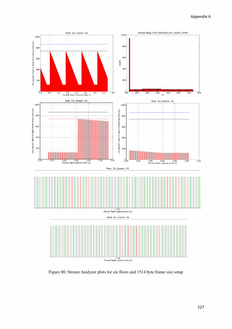
Appendix A
127
Figure 80: Stream Analyzer plots for six flows and 1514 byte frame size setup

Appendix A
128
Figure 81: Stream Analyzer plots for seven flows and 64 byte frame size setup
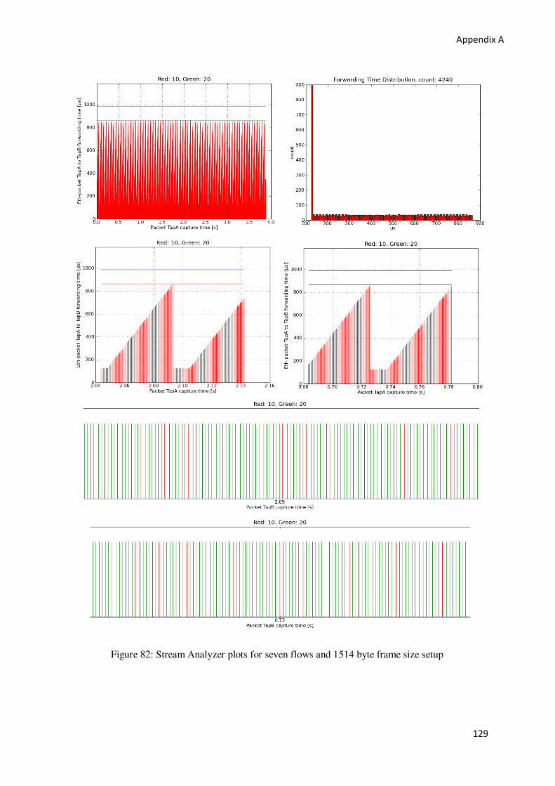
Appendix A
129
Figure 82: Stream Analyzer plots for seven flows and 1514 byte frame size setup

Appendix B: (Compensated) Measured vs. TCN forwarding times
Figure 83: Bar graph comparing TCN Analyzer estimations and measured forwarding times of 64
bytes frame size flows.
Figure 84: TCN Analyzer estimations and (compensated) measured forwarding times of 514 bytes frame size flows.
0
10
20
30
40
50
60
70
1 2 3 4 5 6 7
Fo
rwa
rdin
g t
ime
(μs)
No. of flows
Measured vs. TCN (64 bytes)
Measured
TCN
0
50
100
150
200
250
300
350
400
1 2 3 4 5 6 7
Fo
rwa
rdin
g t
ime
(μs)
No. of flows
Measured vs.TCN (514 bytes)
Measured
TCN
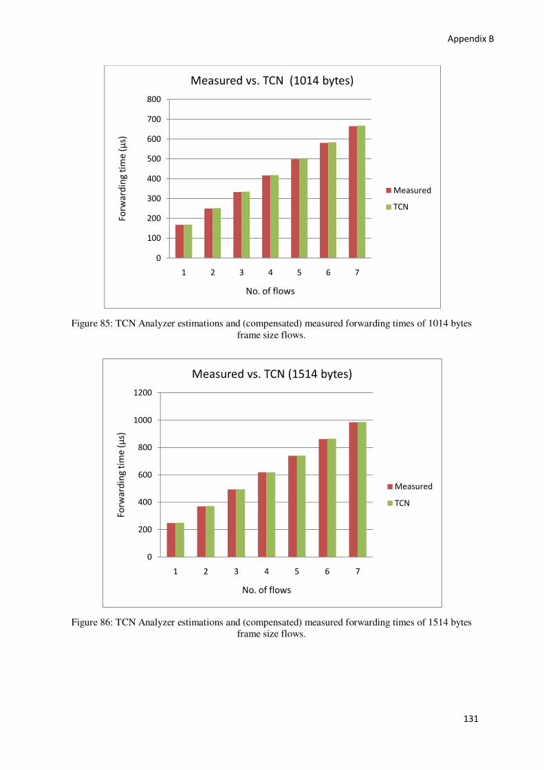
Appendix B
131
Figure 85: TCN Analyzer estimations and (compensated) measured forwarding times of 1014 bytes frame size flows.
Figure 86: TCN Analyzer estimations and (compensated) measured forwarding times of 1514 bytes frame size flows.
0
100
200
300
400
500
600
700
800
1 2 3 4 5 6 7
Fo
rwa
rdin
g t
ime
(μ
s)
No. of flows
Measured vs. TCN (1014 bytes)
Measured
TCN
0
200
400
600
800
1000
1200
1 2 3 4 5 6 7
Fo
rwa
rdin
g t
ime
(μ
s)
No. of flows
Measured vs. TCN (1514 bytes)
Measured
TCN

Appendix C: Drawbacks of Click source
As discussed in section 3.3.4 and section 4.5, we used CAN/Ethernet converter as a UDP frame generator. Initially, during practically verification phase, we used a UDP source built using Click elements. We connected various Click elements to make a UDP source just as we did for Click sink. However, during the measurements we observed that the Click source was nondeterministic in generating UDP frames. Although it was supposed to generate UDP frames at periodic intervals without any interruption, it sent bursts of frames with very high data rate and suffered interruption as well.
Figure 87 shows the forwarding time plots of two measurements when we used Click source as critical UDP frame generator. Here Click source was connected to TAP A port 0 just as CEC1 in other measurements. Observe the burst of frames after an interruption of transmission. Also notice the positive ramp of frames enqueued inside the RedFox switch due to the very high data rate (Large number of packets transmitted in a short period of time).

Appendix C
133
Figure 87: Nondeterministic behavior of Click source.

www.kth.se
TRITA-ICT-EX-2011:175