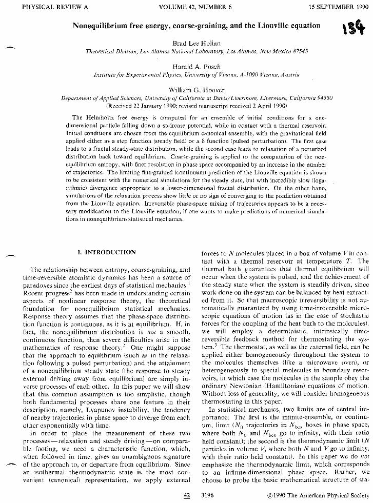
PHYSICAL REVIEW A VOLUME 42, NUMBER 6 15 SEPTEMBER 1990

Nonequilibrium free energy, coarse-graining, and the Liouville equation

Brad Lee Holian Theoretical Division, Los Alamos National Laboratory, Los Alamos, New Mexico 87545

Harald A. Posch Institutefor Experimental Physics, University of Vienna, A-J090 Vienna, Austria

William G. Hoover Department ofApplied Sciences, University of California at Davis/Livermore, Livermore, California 94550

(Received 22 January 1990; revised manuscript received 2 April 1990)

The Helmholtz free energy is computed for an ensemble of initial conditions for a one­dimensional particle falling down a staircase potential, while in contact with a thermal reservoir. Initial conditions are chosen from the equilibrium canonical ensemble, with the gravitational ficld applied either as a step function (steady field) or a 6 function (pulsed perturbation). The first case lcads to a fractal steady-state distribution, while the second case leads to relaxation of a perturbed distribution back toward equilibrium. Coarse-graining is applied to the computation of the non­equilibrium entropy, with finer resolution in phase space accompanied by an increase in the number of trajectories. The limiting fine-grained (continuum) prediction of the Liouville equation is shown to be consistent with the numerical simulations for the steady state, but with incredibly slow (loga­rithmic) divergence appropriate to a lower-dimensional fractal distribution. On the other hand, simulations of the relaxation process show little or no sign of converging to the prediction obtained from the Liouville equation. Irreversible phase-space mixing of trajectories appears to be a neces­sary modification to the Liouville equation, if one wants to make predictions of numerical simula­tions in nonequilibrium statistical mechanics.

I. n,TRODUCTION

The relationship between entropy, coarse-graining, and time-reversible atomistic dynamics has been a source of paradoxes since the earliest days of statistical mechanics. I Recent progress2 has been made in understanding certain aspects of nonlinear response theory, the theoretical foundation for nonequilibrium statistical mechanics. Response theory assumes that the phase-space distribu­tion function is continuous, as it is at equilibrium. If, in fact, the nonequilibrium distribution is not a smooth, continuous function, then severe difficulties arise in the mathematics of response theory. 2 One might suppose that the approach to equilibrium (such as in the relaxa­tion following a pulsed perturbation) and the attainment of a nonequilibrium steady state (the response to steady external driving away from equilibrium) are simply in­verse processes of each other. In this paper we will show that this common assumption is too simplistic, though both fundamental processes share one feature in their description, namely, Lyapunov instability, the tendency of nearby trajectories in phase space to diverge from each other exponentially with time.

In order to place the measurement of these two processes-relaxation and steady driving-on compara­ble footing, we need a characteristic function, which, when followed in time, gives an unambiguous signature

-- of the approach to, or departure from equilibrium. Since an isothermal thermodynamic state is the most con­venient (canonical) representation, we apply external

forces to N molecules placed in a box of volume V in con­tact with a thermal reservoir at temperature T. The thermal bath guarantees that thermal equilibrium will occur when the system is pulsed, and the achievement of the steady state when the system is steadily driven, since work done on the system can be balanced by heat extract­ed from it. So that macroscopic irreversibility is not au­tomatically guaranteed by using time-irreversible micro­scopic equations of motion (as in the case of stochastic forces for the coupling of the heat bath to the molecules), we will employ a deterministic, intrinsically time­reversible feedback method for thermostating the sys­tem. 3 The thermostat, as well as the external field, can be applied either homogeneously throughout the system to the molecules themselves (like a microwave oven), or heterogeneously to special molecules in boundary reser­voirs, in which case the molecules in the sample obey the ordinary Newtonian (Hamiltonian) equations of motion. Without loss of generality, we will consider homogeneous thermostating in this paper.

In statistical mechanics, two limits are of central im­portance: The first is the infinite-ensemble, or continu­um, limit (No trajectories in N box boxes in phase space, where both No and N box go to infinity, with their ratio held constant); the second is the thermodynamic limit (N particles in volume V, where both N and V go to infinity, with their ratio held constant). In this paper we do not emphasize the thermodynamic limit, which corresponds to an infinite-dimensional phase space. Rather, we choose to probe the basic mathematical structure of sta­

42 3196 © 1990 The American Physical Society

42 3205NONEQUILIBRIUM FREE ENERGY, COARSE-GRAINING, AND ...

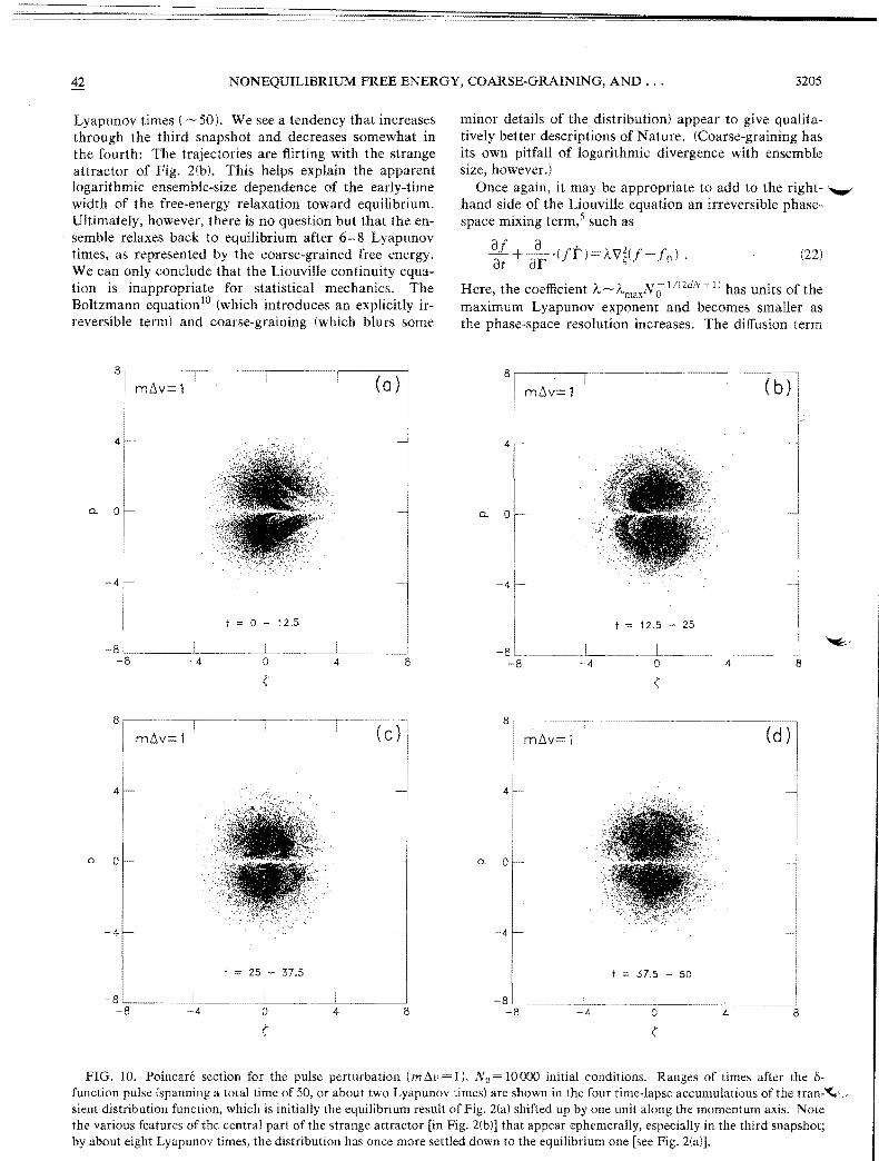
Lyapunov times ( ~ 50). We see a tendency that increases through the third snapshot and decreases somewhat in the fourth: The trajectories are flirting with the strange attractor of Fig. 2(b). This helps explain the apparent logarithmic ensemble-size dependence of the early-time width of the free-energy relaxation toward equilibrium. Ultimately, however, there is no question but that the en­semble relaxes back to equilibrium after 6-8 Lyapunov times, as represented by the coarse-grained free energy. We can only conclude that the Liouville continuity equa­tion is inappropriate for statistical mechanics. The Boltzmann equation lO (which introduces an explicitly ir­reversible term) and coarse-graining (which blurs some

8r-····~-~--,-,-~--~-··~~~-r-~----,

minor details of the distribution) appear to give qualita­tively better descriptions of Nature. (Coarse-graining has its own pitfall of logarithmic divergence with ensemble size, however.)

Once again, it may be appropriate to add to the right- '''-''' hand side of the Liouville equation an irreversible phase­space mixing term,5 such as

aj + a '(jt)= - V~(j ) . (22)at ar Ie s

Here, the coefficient Ie - "'rna/V0 1 Ii 2dN + 1: has units of the maximum Lyapunov exponent and becomes smaller as the phase-space resolution increases. The diffusion term

8 I .-...--~.... ..~..---:

4

0

4

CL CL 0

CL 0 CL 0

-4 -4

25 - 37.5

-8, ~ .. _~._ -8~....___ ....~_._.~.. _~.... .1.____._......L ___~ -8 -4 0 4 8 -8 -4 0 4 8

( (

FIG. 10. Poincare section for the pulse perturbation (mAv 1), No=10000 initial conditions. Ranges of times after the 8­function pulse (spanning a total time of 50, or about two Lyapunov times) are shown in the four time-lapse accumulations of the tran-'<e., sient distribution function, which is initially the equilibrium result of Fig. 2(a) shifted up by one unit along the momentum axis. Note the various features of the central part of the strange attractor [in Fig. 2(bl] that appear ephemerally, especialIy in the third snapshot; by about eight Lyapunov times, the distribution has once more settled down to the equilibrium one [see 2(a)].

3206 42 HOLIAN, POSCH, AND HOOVER

in S mImIcs the phase-space mixing that occurs so of the entropy, as it does for mechanical observables like dramatically in Fig. 10. When (22) is applied to the the energy. However, the fractal nature of nonequilibri­rate of change of mechanical observables (including the um steady-state distribution functions requires almost an thermostating energy that is quadratic in ~), the opera­.~ tions of time derivative d Idt and ensemble average ( ) commute. On the other hand, there arise additional terms for the entropy, or the free energy [Eq. (19)]:

A=(J)·x AkT f dr ~[(V~~f)2+dNs~f(V~~f)],

(23)

where ~f The first two terms are of order X2 and the last is of order , consequently, the correction to the Liouville-equation prediction is negative, at least for small fields. The last term can be of either sign and therefore contribute to the oscillatory behavior of ~ A [see Fig. 8(a)]. Qualitatively, these terms can account for the coarse-graining and phase-space mixing effects in both the steady- and pulsed-field results for the nonequili­brium free energy of the Galton staircase.

VI. CONCLUSIONS

For thermostated systems, the Helmholtz free energy is the appropriate charaeteristic function to show either the departure from, or return to, equilibrium. Unfortunately, predictions based on the Liouville continuity equation must be compared with finer and finer coarse-grained realizations of the engropy. For nonequilibrium steady states, this comparison is doomed because of the incredi­

~. bly slow (logarithmic) divergence of entropy with ensem­ble size. It would seem intuitive that an ensemble of a few hundred experiments ought to suffice for a realization

infinite amount of information, or resolution, for the en­tropy .

It turns out that the really crucial test for the predic­tions using the Liouville equation is the relaxation to equilibrium from a pulsed external field, where the free energy is predicted to be a step function. On the con­trary, numerical simulations show that relaxation to equi­librium occurs for the coarse-grained free energy after about eight Lyapunov times, regardless of ensemble size. Also, the distribution function recalls-fleetingly-the face of the attractor under steady driving, but finally it becomes once again a smooth, continuous func­tion. Thus, any similarity between the processes of relax­ation and the achievement of the nonequilibrium steady state is only transient. The notion that they are inverses of each other is an oversimplification.

Finally, we are forced to conclude that the mixing of trajectories in the process of equilibration is not described realistically by the Liouville equation. Phase-space mix­ing can be incorporated into a modified Liouville equa­tion, which captures the essence of coarse-graining in an empirical way.

ACKNOWLEDGMENTS

We acknowledge very useful discussions with Kyozi Kawasaki, Eddie Cohen, Jerry Erpenbeck, Peter Milonni, Jim Hammerberg, Chris Patterson, Nicolas van Kampen, and David Chandler. Many of the focal points of this work originated in discussions with Ilya Prigogine.

IJ. W. Gibbs, in The Collected Works ofJ. Willard Gibbs mans, New York, 1931), Vol. 2.

2B. L. Holian, G. Ciccotti, W. G. Hoover, B. Moran, and H. A. Posch, Phys. Rev. A 39,5414 (1989); B. L. Holian, W. G. Ho­over, and H. A. Posch, Phys. Rev. Lett. 59, 10 (1987).

Nose, Mol. Phys. 52, 255 (1984); J. Chern. Phys. 81, 511 (1984); W. G. Hoover, Phys. Rev. A 31, 1695 (1985).

4B. J. Alder and T. Wainwright, in Transport Processes in Sta­tistical Mechanics, edited by 1. Prigogine (Interscience, New York, 1958).

5B. L. Holian, Phys. Rev. A 34, 4238 (1986). 6M. C. Mackey, Rev. Mod. Phys. 61, 981 (1989).

for example, D. A. Mcquarrie, Statistical .Mechanics (Harper and Row, New York, 1976), pp. 35-40.

8W. G. Hoover, H. A. Posch, B. L. Holian, M. J. Gillan, M. Mareschal, and C. Massobrio, Molecular Simulations 1, 79 (1987).

9H. A. Posch, \V. G. Hoover, and B. L. Holian, Ber. DUIl:;t:lIgt:~. Phys. Chern. 94, 250 (1990).

1OL. Boltzmann, Scientific Treatises of Ludwig Boltzmann, edit­ed by F. Hasenohrl (Barth, Leipzig, 1909); see also The Boltzmann Transport Equation, edited by W. Thirring and E. Go, D. Cohen (Springer, Vienna, 1973).

""""".

42 NONEQUILIBRIUM FREE ENERGY, COARSE-GRAINING, AND ... 3197

tistkal'mechanics by studying the limit of an infinite en­semb'le and its representation as a continuous distribution function in a finite-dimensional phase space.

Since the systems of interest are not thermally isolated, the initial conditions for the non equilibrium experiments, performed under identical boundary conditions (external time-dependent driving), will be selected from an equilib­rium canonical ensemble. If the system were thermally isolated, the characteristic function would be the entropy S, which would be a maximum at equilibrium. Over thir­ty years ago, Alder and Wainwright,4 in a pioneering molecular-dynamics computer simulation, showed that the Boltzmann .'lI function for a dilute gas, which is - S / k (k is Boltzmann's constant), indeed decays to a minimum at equilibrium. However, for a finite, thermo­stated system, the Helmholtz free energy A is the ap­propriate characteristic function, and it reaches a minimum at equilibrium.

The Helmholtz free energy is given by

A (1)= E (t)- TS (t)= - kTlnZ (t) , (1)

where E is the energy of the system and Z is, by definition, the partition function. How do we measure such a thing for an ensemble of trajectories7

The energy E, like all mechanical observables, is most accurately and conveniently measured in the Lagrangian (Heisenberg), or co-moving, frame of reference in phase space. If all coordinates, momenta, and the thermostat heat-flow variable are collected into the vector r, then a trajectory in the multidimensional phase space is represented by ri(t), where i ranges from 1 to No, the en­semble size (number of different initial conditions). The energy function along a trajectory is Hi(t)=H(rj(t)), and the ensemble average is

1"/0

E(t) (H(t)= 1 _ 2: Hi(t)No i=l

-> f dr jo(r)H(r(t» . (2)

The continuum limit has been taken in order to obtain the latter expression,2 in which the equilibrium (canoni­cal) distribution function provides the weight of each tra­jectory and is given by

(3)

with [3= 1/kT and the equilibrium partition function given by Zo= f drexp( -[3H).

The alternative way of looking at the ensemble average E is in the Eulerian (Schrodinger), or space-fixed, frame, where the No trajectories are counted into N box boxes fixed in phase space (box j is centered at r j with volume arj , and j ranges from 1 to Nbox )' Then,

1 Non"!.

E(t) (H(t)= 'V 2: Hjn/f) 1 o} I

Nb"x = ~ H,P(t)

J{., }}' j 1

-+ f dr H(rJj(r,t) . (4)

Again, the continuum limit has been taken to get the latter expression.2 The occupation number in box j is nj (t); the number of trajectories is

N box

No 2: nj(t) (5) j I

and, therefore, the probability of occupation in box j is Pj(t) nj(t)/No, which is related to the distribution function j by p}(t):::o:j(rj,t)arj • (Note that both P and j are normalized to unity.) The number of boxes N box is chosen so that the average occupation number in each box is <n ) /Nbox , a fixed ratio when we take the continuum limit. Because the boxes are coarse­grained in practical realizations, ensemble averages in the Eulerian picture are subject to more statistical noise than in the Lagrangian picture.

On the other hand, for the entropy, a measure of the phase-space probability density itself, there is no choice but to compute it in the Eulerian frame:

-.;,-k f dr j(r,t)lnj(r,t) kOnj(t) . (6)

The first line is Boltzmann's most famous equation. It states that the total entropy of the ensemble (NoS) is Boltzmann's constant k times the logarithm of the num­ber of ways U(No,Nbox) that No trajectories can be distri­buted among N box boxes. Only the most probable configuration (nj J need be considered because of the huge factorials involved (even for only 100 trajectories in 100 boxes); therefore, Stirling's approximation to InNo! holds..The last line is obtained by taking the continuum limit, although we have arbitrarily thrown away a subtle, but well-known coarse-graining singularity, namely, -k lnar. Usually, this singularity in the continuum ex­pression for the entropy is dismissed as being trivial, since we say that we are only interested in entropy differences. Indeed, in this paper, we will report differences from equilibrium for each ensemble size.

While the entropy of a finite, thermostated system may ­oscillate rather wildly, the free energy either approaches (more or less monotonically) a minimum at equilibrium ( A 0) or rises monotonically when the system is driven away from equilibrium:

HOLIAN, POSCH, AND HOOVER3198 42

kTln?(t)AA(t) A(t) Ao= Zo

N box Pj(t)=kT ~ P(t)ln~--

k.; j pO j= I J

f(r,t)--'> kT drf(r t)ln·· - ..~ >0 (7)f , fo(r) -- ,

implying, as Gibbs showed, I that the accessible number of states at equilibrium is greater than under any other circumstance.

Earlier work identified the negative of Eq. (7) with T t~m~s "the nonequilib~ium entropy, relative to the equi­hbnum distribution,") which was shown in numerical realizations of thermal equilibration to rise unambiguous­ly toward equilibrium. In a very interesting recent review article, which concentrates primarily on the closely relat­ed topic of irreversible dynamical systems, Mackev has independently made the same identification, except t~ call it the "conditional entropy.,,6 From the preceding dis­cussion, however, it is clear that we should more properly identify the characteristic function in Eq. (7) as the free­energy difference relative to the equilibrium value.

We should also note that a common way to derive7 the equilibrium canonical distribution function fo is to max­imize the entropy variationally with respect to fa, subject to two constraints: (1) that the total energy of the ensem­ble be constant and (2) that be normalized. The latter constraint is eminently reasonable: It is nonsensical to imagine that trajectories can be either created or lost. The mathematical constraint on the total energy of the ensemble, however, has a serious physical flaw in its in­terpretation, namely, that the elements of the ensemble exchange energy among themselves and thereby interact with each other-a violation of our fundamental assump­tion of noninteracting trajectories. In fact, the correct physical picture of the thermal reservoir is that each member of the ensemble is submerged in it, and energy is exchanged between this heat bath and each element in­dependently. Thus, the ensemble average can exhibit nonequilibrium fluctuations-even as we approach the continuum limit. It is only in the thermodynamic limit that fluctuations for each member of the ensemble disap­pear; only then is total energy conservation for the en­semble a good approximation. Since the formalism of statistical mechanics applies to systems with few degrees of freedom, we see clearly now that one must first take the continuum limit, and then the thermodvnamic limit if necessary. Taking the reverse order of limits can b~ very misleading.

The best way to think about the derivation of f 0 is to imagine minimizing the free energy variationally with respect to f 0' subject only to the constraint that fa be normalized. With this interpretation for a thermostated- system with a finite number of particles, we see that, away from equilibrium, both the energy and entropy can

guous global minimum at equilibrium, except for random fluctuations, is the free energy.

II. ENSEMBLE DYNA,\HCS AND THE LIOl;VILLE EQUATIO~

In the framework of the NVT or canonical ensemble, we now consider generalizable equations of motion for N particles in a d-dimensional box of volume V (periodic boundary conditions) in contact with a thermal reservoir ~t temperature T. In addition, we provide for the opera­tIon of an external driving force XU). (For simplicity, we assume that both the thermostat and X act homogene­ously throughout V.) We will be concerned with two ~ases: (1) step-function driving, X(t)=X8(t to),lead­mg to a non equilibrium steady-state response; and (2) 0­

function ~p.ulsed perturbation) driving, X(t) = Apo\t - to), glvmg a response that relaxes back to equilibri­um. For the example of mass transport, such as conduc­tivity under an imposed electric or gravitational field, the equations of motion are

(Sa) hr,t)= (8b)

v(p'pldN mkT-l) . (8cl

The phase space is r=(q,p,~l, where q are the dN parti­cle coordinates, p are the dN particle momenta, and ~ is the dimensionless heat-flow variable that describes the relative magnitude and direction of heat flow from the particles to the thennal reservoir (positive (; means the particles lose kinetic energy to the bath and negative means the bath heats them up). Thus, the so-called "fric­tion" coefficient can have either sign, in fact. The cou­pling of the heat bath to particles is governed by the rate-of-thermostating parameter v: v=o gives the usual Newtonian (Hamiltonian) equations of motion; in order for the thermostating to be efficient, it is best to choose v to be on the order of the mean collision rate of the parti­cles. The response of the particles to the thermostat is in the nature of integral feedback,3 i.e., on the timescale of I Iv. Furthermore, Eq. (8c) guarantees that the long-time average ofthe kinetic energy K(p) p·p/2m will always be t-,dNkT, even at a nonequilibrium steady state. [Under the equilibrium thermostated equations of motion, the canonical distribution fa is a stationary solution to the Liouville continuity equation, to be presented later. Thus, for sufficiently mixing systems, this thermostat guarantees that the long-time average of an observable is equivalent to a canonical-ensemble average,3 since any equilibrium trajectory will eventually visit every box in phase space, with probability fa(rJdr.] From the total potential energy <1>( q), we obtain the internal forces F(q) -aq>(q)/aq.

The total energy of the system of particles and ther­mostat is

fluctuate, so that the entropy is not necessarily a global (9) maximum at equilibrium, as it is in isolated systems. In­stead, the characteristic function that attains an unambi- which includes a contribution from the thermostat of or­

42 NONEQUILIBRIUM FREE ENERGY, COARSE-GRAINING, AND ... 3199

der unity compared to the extensive (order l{) quantities K and tP, since U;2 1/dN. Note also that the work done by the thermostat is quadratic in the heat-flow vari­able. The rate of change of H for the equations of motion, Eqs. (8), is therefore

Ii -dNkTv~+J'X, (10)

where the flux is J=plm in response to the external force X. Thus, the macroscopic equation of motion for E is

j; (Ii) Q W, (11)

where the rate of heat flow into the system is

Q=~dNkTv<~> , (12)

and the rate of work done by the system is

W=-(J)·X. (13)

For the cases we are interested in, both of these quantities are typically negative, i.e., work is done on the system and heat is extracted from it. For example, at the steady state, the flux is given by the transport coefficient ex (con­ductivity in our mass-transport example), which is in gen­eral a positive-definite nonlinear function of X, times the field X: (J)ss=g(X)'X, showingthat Wss -exX2 <0. From the equations of motion, we see that v{ ~) ss is a positive frictional damping coefficient, so that

Qss=-dNkTv<S>ss<O.

Since =~, we expect to find in numerical simulations that Qss Wss' Equation (11) embodies the first law of thermodynamics.

The macroscopic equation of motion for the entropy of the ensemble necessarily involves not just a simple aver­age over independent trajectories, but rather a probabilis­tic measure of the density of trajectories in all of phase space. For this, we need the Liouville continuity equa­tion in its full generality to describe the flow of trajec­tories:

(14)

The swarm of trajectories in the (2dN + 1 )-dimensional phase space is thus imagined to be a peculiar fluid of noninteracting "particles.,,2 The Liouville equation can also be written in the form

cJ[+fA=O (15)dt '

where the logarithmic expansion rate of local phase-space volume elements is

a . A= ar ·nr,t) . (16)

From the equations of motion [Eqs. (8)], we see that A has no explicit field dependence and therefore no explicit time dependence:

aA= (17)ap 'p= -dNv~ .

(This is the usual case for most nonequilibrium processes, though one could imagine bizarre equations of motion that would lead to more exotic expressions for A.) Ap­plying the Liouville equation S = - k ( lnf ), we find that

to the entropy

TS= kT(lnf)

=kT(A)

-dNkTv(~)

Q, (18)

where we rearrange Eq. (15) to read lnf=j If -A. Equation (18) embodies the mathematical statement of the second law of thermodynamics, as predicted by the Liouville equation. This leads to a remarkably simple prediction for the behavior of the Helmholtz free energy:

A TS

=(Q-W) Q

W

(J)·X, (19)

or, since equilibrium is imagined to prevail for ~ 00 < t < to, so that A (to)= Ao, we have

. (20)

The case of the pulsed perturbation, X( t) = .6.p8( t - to), deserves particular attention; there,

For t o-, to, and t o+, (p(t) is 0, +.6.p, and .6.p, respec­tively, so that .6. A (t > to) .6.p 12 /2;n. Since the distribu­tion function f( r, to+ ) is the equilibrium f 0 perturbed by translating the momentum origin, fo(q,p .6.p,~), the entropy is initially unaffected by the b-function external force, For these thermostated systems, the surprising thing is that the Liouville equation for f predicts a step­function change in the free energy, with no subsequent re­laxation back to equilibrium. For an isolated system, the equivalent conundrum (Gibb's paradox) is that the entro­py never changes as the system relaxes. 1

If we coarse-grain the available phase space into N box

discrete boxes (.6.r) and make the resolution finer and finer (Nbox - 00 J, taking more and more initial conditions (No - 00 ), with the ratio of trajectories to boxes No INbox

fixed, do we find that the free energy converges or diverges? And is this phase-space convergence (diver­gence) rapid or slow? What happens as the system ap­proaches the steady state under step-function driving? Does the system, when perturbed by a o-function pulse, ever equilibrate? In what sense, if any, are these two nonequilibrium processes equivalent? These questions are fundamental to the application of statistical mechan­ics to the real world.

3200

4

HOLIAN, POSCH, AND HOOVER

III. THE GALTON STAIRCASE

We choose as an example8 of the equations of motion, Eqs. (8), a single particle on a one-dimensional (lD) "washboard" substrate (a sinusoidal potential) with spa­tial periodicity 21i:

<f>(q)= I -cosq , (21)

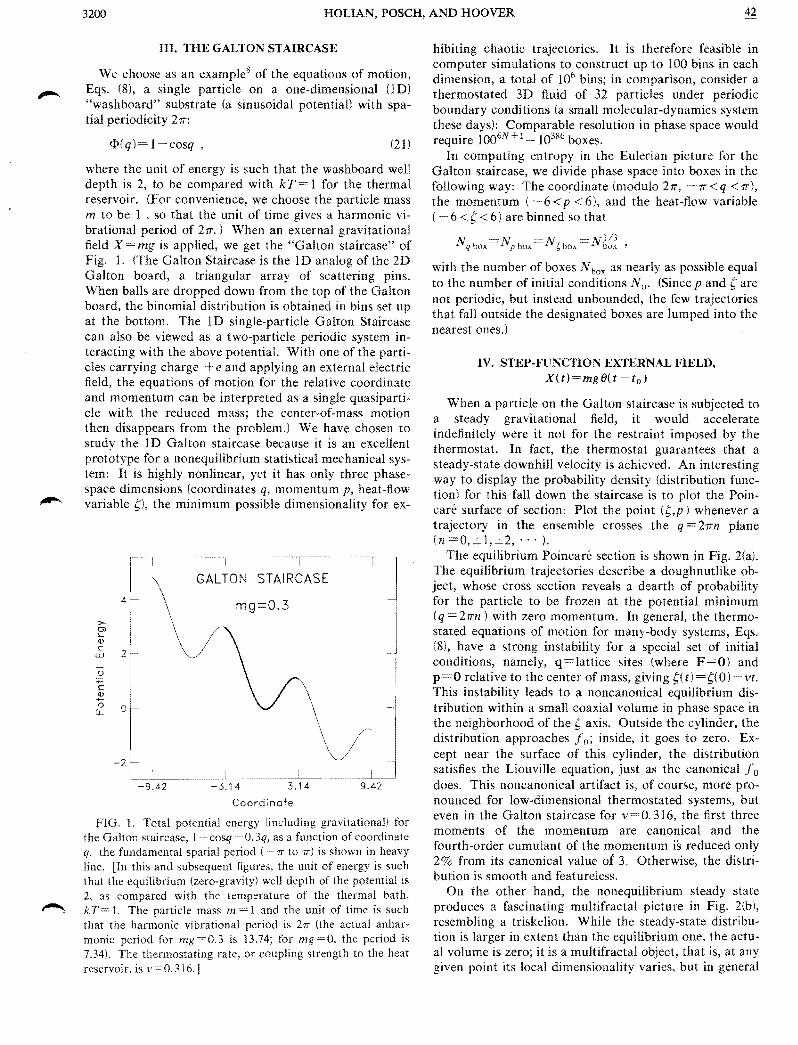
where the unit of energy is such that the washboard well depth is 2, to be compared with kT= 1 for the thermal reservoir. (For convenience, we choose the particle mass m to be I , so that the unit of time gives a harmonic vi­brational period of 21T.) When an external gravitational field X = mg is applied, we get the "GaIton staircase" of Fig. 1. (The Galton Staircase is the I D analog of the 2D Galton board, a triangular array of scattering pins. When balls are dropped down from the top of the Galton board, the binomial distribution is obtained in bins set up at the bottom. The ID single-particle Galton Staircase can also be viewed as a two-particle periodic system in­teracting with the above potential. With one of the parti­cles carrying charge + e and applying an external electric field, the equations of motion for the relative coordinate and momentum can be interpreted as a single quasiparti­cle with the reduced mass; the center-of-mass motion then disappears from the problem.) We have chosen to study the ID Galton staircase because it is an excellent prot~type for a nonequilibrium statistical mechanical sys­tem: It is highly nonlinear, yet it has only three phase­space dimensions (coordinates q, momentum p, heat-flow variable (;), the minimum possible dimensionality for ex-

GALTON STAIRCASE

mg=O.3

o-C <l>

-0 o ~

-2

-9.42 -3.14 3.14 9.42

Coordinale

FIG. 1. Total potential energy (including gravitational) for the Galton staircase, l-cosq -0. 3q, as a function of coordinate q. the fundamental spatial period (-rr to rr) is shown in heavy line. [In this and subsequent figures, the unit of energy is ~uch that the equilibrium (zero-gravity) well depth of the potentIal IS

2, as compared with the temperature of the thermal bath, kT= 1. The particle mass m 1 and the unit of tiine is such that the harmonic vibrational period is 2rr (the actual anhar­monic period for mg=0.3 is 13.74; for mg=O, the period is 7.34). The thermostating rate, or coupling strength to the heat reservoir, is v=0.316.]

hibiting chaotic trajectories. It is therefore feasible in computer simulations to construct up to 100 bins in each dimension, a total of 106 bins; in comparison, consider a thermostated 3D fluid of 32 particles under periodic boundar v conditions (a small molecular-dynamics system these days); Comparable resolution in phase space would require I 006J11 +1 = 10386 boxes.

In computing entropy in the Eulerian picture for the Galton staircase, we divide phase space into boxes in the following way: The coordinate (modulo 21T, -1i < q < 1T), the momentum ( 6 <P < 6), and the heat-flow variable ( 6 < (; < 6) are binned 50 that

with the number of boxes N box as nearly as possible equal to the number of initial conditions No. (Since p and (; are not periodic, but instead unbounded, the few trajectories that fall outside the designated boxes are lumped into the nearest ones.)

IV. STEP-FUNCTION EXTERNAL FIELD, X(t)=mglJ(t -to)

When a particle on the Galton staircase is subjected to a steady gravitational field, it would accelerate indefinitely were it not for the restraint imposed by the thermostat. In fact, the thermostat guarantees that a steady-state downhill velocity is achieved. An interesting way to display the probability density (distribution func­tion) for this fall down the staircase is to plot the Poin­canS surface of section: Plot the point ({;,p) whenever a trajectory in the ensemble crosses the q 21in plane (n O,±1,=2,···).

The equilibrium Poincare section is shown in Fig. 2(a). The equilibrium trajectories describe a doughnutlike ob­ject, whose cross section reveals a dearth of probability for the particle to be frozen at the potential minimum (q = 21ifl ) with zero momentum. In general, the thermo­stated equations of motion for many-body systems, Eqs. (8), have a strong instability for a special set of initial conditions, namely, q=lattice sites (where F=O) and p 0 relative to the center of mass, giving {;(t)={;(O) vt. This instability leads to a non canonical equilibrium dis­tribution within a small coaxial volume in phase space in the neighborhood of the {; axis. Outside the cylinder, the distribution approaches f 0; inside, it goes to zero. Ex­cept near the surface of this cylinder, the distribution satisfies the Liouville equation, just as the canonical fo does. This noncailonical artifact is, of course, more pro­nounced for low-dimensional thermostated systems, but even in the Galton staircase for v=O.316, the first three moments of the momentum are canonical and the fourth-order cumulant of the momentum is reduced only 2% from its canonical value 01 3. Otherwise, the distri­bution is smooth and featureless.

On the other hand, the nonequilibrium steady state produces a fascinating multifractal picture in . ~(b), resembling a triskelion. While the steady-state dlstnbu­tion is larger in extent than the equilibrium one, the actu­al volume is zero; it is a multifractal object, that is, at any given point its local dimensionality varies, but in general

-42 3201NONEQUILIBRIUM FREE ENERGY, COARSE-GRAINING, AND ...

is nonintegral and less than three, the dimensionality of f o' Of course, at the steady state the distribution abso­lutely cannot have an overall dimensionality greater than the full phase space-that would be absurd. On the oth­er hand, the distribution clearly does not shrink to a limit cycle of dimension 2, either. In fact, the dimensionality for mg=0.3 and v=0.316 has been measured8

,9 to be 2.47. (That is, the Poincare section in Fig. 2(b) is ~ 1. 5

dimensional, as measured by the average logarithm of the local area around a point, divided by the logarithm of the radial resolution, in the limit of zero radius.)

The dimensionality of the steady-state distribution is consistent with our arguments about A, the local loga­rithmic expansion rate of phase-space volume, and its re­lationship to the heat flow. That is, <A ) S8 <0, so that the volume of the distribution must shrink to zero. The

8

mg=O

4

0. 0

-4

-8-8 88 -8-8

mg=O.3

4

-4

8,-----------------------------~

REPELLOR ~ ATTRACTOR

4

0. 0

-4

FIG. 2. Poincare surface of section for the Galton staircase, where the momentum p is plotted vs the heat-flow coefficient ~ when­ever the coordinate q reaches an integral multiple of 2rr. (a) At equilibrium (mg =0), an ensemble of No = 10 000 initial conditions generates the Poincare section at an average rate of 13.6 points per trajectory in a time of 50; note the smoothness of the equilibrium distribution. (b) At the steady state (mg =0. 3), all trajectories collapse onto the multifractal strange attractor. After a time of ~ 2000 at the steady state, the Poincare section is accumulated over a time of 50 at an average rate of 7.3 points per trajectory. The phase-space fractal dimensionality of the attractor is 2.47 (see Ref. 9). (c) By performing the time-reversal transformation p ---+ - p, -S") on the No 10 000 ensemble at a time of ~ 2000 after the establishment of the steady state, the strange repellor is .£' obtained as a Poincare section, which is accumulated for approximately one Lyapunov time (25). The repellor states are Lyapunov unstable, persisting for only about two Lyapunov times, during which the second law is violated (negative conductivity); here, after one Lyapunov time, faint wisps that destroy the inversion symmetry of the repellor can already be seen, as some trajectories begin to head again for the attractor-a proeess completed for virtually the entire ensemble after about four Lyapunov times.

3202 42 HOLIAN, POSCH, AND HOOVER

Lyapunov exponents,9 one for each dimension in phase space for this system, are +0.0393,0, and 0.0842. The three cumulative sums represent exponential rates at

~. which one-, two-, and three-dimensional elements in phase space grow with time; in particular, the sum of all the Lyapunov exponents is ~)"i (A) sS' Thus, while the attractor to which the distribution collapses at the steady state has zero volume, nearby pairs of trajectories diverge exponentially with time from each other because Amax> 0; hence the name "strange attractor."

In the pantheon of paradoxes in statistical mechanics, Loschmidt's paradox of macroscopic irreversibility aris­ing from reversible microscopic equations of motion is represented by the so-called "strange repellor.,,2 It is ob­tained by reversing velocities (and the heat-flow variable) after training the ensemble of trajectories onto the strange attractor-the time-reversal transformation, t~+-t, q--+q, p--+-p, ;. The reversed trajec­tories obey the same equations of motion, but the miracu­lous thing is, the average flux is reversed - the particle faUs uphill on average-and the transport coefficient (conductivity) is negative.

The resolution to this paradoxical violation of our in­tuition and experience (the second law of thermodynam­ics) is that the volume occupied by these strange repellor states is identically zero (like the attractor), so that the probability of actually observing such a violation of the second law is identically zero. Moreover, these states have the same Lyapunov exponents, except for sign:

. + 0.0842, 0, and - O. 0393. Thus, the repellor is absolute­,.... ly unstable9 on a time scale of 1IAmax ~ 25. The states

that are approximately on the repellor soon find their way back to the attractor, as shown in Fig. 2(c). The wispy, non-repellor-like features on this Poincare section collected within a time of 25 after the time-reversal trans­formation [which results in a 1800 rotation of Fig. 2(bl] are the most unstable trajectories, which are already heading back to the attractor. By a time of 50, the aver­age flux has gone from - (J ) ss to zero, and by a time 100, the flux has returned to (J) ss' This feature is in­sensitive to the time step for the central difference ap­proximation to the equations of motion, as well as to the length of time spent at the steady state before the time re­versal. (In contrast, after an impulse to an equilibrium ensemble, we have observed that reversibility depends weakly, i.e., logarithmically, on the time step. In princi­ple, the reversibility time can be made arbitrarily long by using accurate and intrinsically time-reversible algo­rithms, such as central differences, and by using longer and longer computer word lengths. In practice, we have found this to be severely subject to the law of diminishing returns.) Generally, the entropy shows significantly more sensitivity to reversibility than mechanical observables such as the energy.

The steady-state plateau values of mechanical observ­abIes are attained on a time scale of 6-8 Lyapunov times

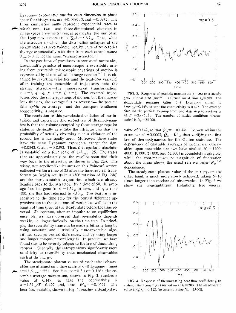
~ (1 -25). For X=mg=0.3 (v=0.316), the en­semble average momentum, shown in Fig. 3, reaches a value of 0.149, so that the conductivity is a= (J )ssIX=0.497 and, thus, Wss -0.0447. The heat-flow variable, shown in Fig. 4, reaches a steady-state

0.5

0.4

1\ > E v

0,3

0.2

0,1

0.0

mg::::O.3

, ~ ~

) i \1 (VWAJ'~~ ~ If'tJ

'\

~0.1 L_~_L~~~~~~ ...~~~~..... __~~-L... _~__ 200 250 300 350 400 450 500 550 600

Time

FIG. 3. Response of particle momentum p mv to a steady gravitational field (mg =0. 3) turned on at time to = 200. The steady-state response (after 6-8 Lyapunov times) is <mv 149, so that the conductivity is 0.497. The average time for the particle to jump from one stair step to another is 42.17 = 2IT / <v The number of initial conditions (trajec­tories) is No = 25 000.

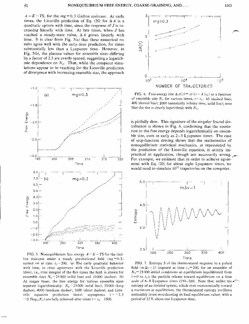
value of 0.142, so that Qss = -0.0449. To well within the error bar of ±0.0003, Qss W ' thus verifying the first ss law of thermodynamics for the Galton staircase. The dependence of ensemble averages of mechanical observ­abies upon ensemble size (we have studied No = 1600, 4000, 10 000, 25000, and 62 500 l is completely negligible, while the root-mean-square magnitude of fluctuation about the mean shows the usual relative order N;;l!2 dependence.

The steady-state plateau value of the entropy, on the other hand, is much more slowly achieved, taking 5 10 times longer than mechanical observables. In Fig. 5 we show the nonequilibrium Helmholtz free energy,

0.5

0.4

0.3

/\ v 0.2 v

Time

f\ ;\ J\

\ 1\ /: II f\( \~il/tllI I Vi I \1 V' " 0.1 I \I ~ v

\ I I \;

II 0.0 II,

mg=O.3

II ~

I II

FIG. 4. Response of thermostating heat-flow coefficient Sto a steady field (mg=0.3) turned on at to=200. The steady-state value is <s) ss = 0.142, for ensemble size No = 25000.

NONEQUlLlBRIUM FREE ENERGY, COARSE-GRAINING, AND ...42 3203

A =E TS, for the mg=0.3 Galton staircase. At early times, the Liouville prediction of Eq. (20) for AA is a quadratic upturn with time, since the response of J is in­creasing linearly with time. At late times, when J has reached a steady-state value, AA grows linearly with time. It is clear from Fig. 5(a) that these numerical re­sults agree well with the early-time prediction, for times substantially less than a Lyapunov time. However, in Fig. 5(b), the plateau values for ensemble sizes differing by a factor of 2.5 are evenly spaced, suggesting a logarith­mic dependence on No. Thus, while the computer simu­lations appear to be reaching for the Liouville prediction of divergence with increasing ensemble size, the approach

-1.0

(a) mg 0.3

-1.5

>­0> ' ­<l1 C

UJ -2.0 <l1 <l1...

'"'­

-2.5

-3.0 195 220

Time

8.0

7.0 mg:::0.3

6.0

5.0

>- 4.0 0>... (I)

c 3.0 w (I) 2.0 (I)

' ­'"'- 1.0

0.0

-1.0

-2.0

-3.0

Time

FIG. 5. Nonequilibrium free energy A = E TS for the Gal­ton staircase under a steady gravitational field (mg =0.3) turned on at time to =200. (a) The early quadratic behavior with time, in close agreement with the Liouville prediction (dots), i.e., time integral of the flux times the field, is shown for ensemble sizes No = 25000 (solid line) and 10 000 (dashes). (b) At longer times, the free energy for various ensemble sizes separate logarithmically: No = 25000 (solid line), 10 000 (long dashes), 4000 (medium dashes), 1600 (short dashes), and Liou­ville equation prediction (dots); asymptotes ( - ~ 2. 3 +0. 510g 1ONo ) are fully achieved after times t - to + 1500.

mg=0.3

.­2

O~__...L-~_... L~~.L~__ ~ _~-L_~~__~

103 104 ; 05

NUMBER OF TRAJECTORIES

FIG. 6. Free-energy rise il A (t) A (t) ~ A (to) as a function of ensemble size No for various times, t to: 65 (dashed line), 400 (dotted line), 2000 (essentially infinite time, solid line); note that the rise is clearly logarithmic with No.

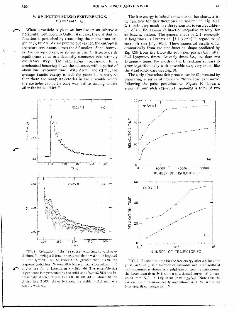
is pitifully slow. This signature of the singular fractal dis­tribution is shown in Fig. 6, confirming that the resolu­tion in the free energy depends logarithmically on ensem­ble size, even as early as 2-3 Lyapunov times. The case of step-function driving shows that the mathematics of non equilibrium statistical mechanics, as represented by the prediction of the Liouville equation, is utterly im­practical in application, though not necessarily wrong. ~ For example, we estimate that in order to achieve agree­ment with Eq. (20) for about eight Lyapunov times, we would need to simulate 1015 trajectories on the computer.

5.0 ,- ~I~- ----r-~-r---···-· ­mLlv= 1

4.5

>­Q. o... ~

c w

4.0

200 300

Time FIG. 7. Entropy S of the thermostated response to a pulsed

field (milv=l) imposed at time to = 200, for an ensemble of No =25 000 initial conditions at equilibrium (equilibrated from t =0 to to); the particle relaxes toward equilibrium on a time scale of 6-8 Lyapunov times (150-200). Note that, unlike the r~, entropy of an isolated system, which rises monotonically toward. a maximum at equilibrium, the thermostated entropy oscillates noticeably (even overshooting its final equilibrium value), with a period of 22.9, about one Lyapunov time.

HOLIAN, POSCH, AND HOOVER3204 42

V. I)-FUNCTION PULSED PERTURBATION, X(t)=dpl)( t - to)

r"' When a particle is given an impulse on an otherwise horizontal (equilibrium) Galton staircase, the distribution function is perturbed by translating the momentum ori­gin of f 0 by l:!..p. As we pointed out earlier, the entropy is therefore continuous across the 8 function. Soon, howev­er, the entropy drops, as shown in Fig. 7. It recovers its equilibrium value in a decidedly non monotonic, strongly oscillatory way. The oscillations correspond to a mechanical bouncing down the staircase, with a period of about one Lyapunov time. With l:!..p = I and kT= 1, the average kinetic energy is half the potential barrier, so that there are many trajectories in the ensemble where the particles can fall a long way before coming to rest after the initial "kick." '

-2.4

-2.8

Time

:a

0.50

i 0.25;­

0.00

mCw= 1

350

Time

FIG. 8. Relaxation of the free energy with time toward equi­librium, following a 8-function external field (In LlV = 1 ) imposed at time to=200. (a) At times t to greater than .~ 150, the response (solid line, No = 62500) behaves like a Lorentzian (the

" circles are for a Lorentzian 7=56). (b) The ensemble-size dependence is represented by the solid line (No =62 500) and in­creasingly shorter dashes (25000, 10 000, 4000 \, down to the dotted line (1600). At early times, the width of LlA increases weakly with No.

The free energy is indeed a much smoother characteris­tic function for this thermostated system: in Fig. 8(a), AA looks very much like the relaxation toward equilibri­um of the Boltzmann j{ function (negative entropy) for an isolated system. The general shape of dA, especially at long times, is Lorentzian, [1 +(t / T)2] ~ J, regardless of ensemble size [Fig. 8(bl]. These numerical results differ dramatically from the step-function shape predicted by Eq. (20) from the Liouville equation, particularly after 6-8 Lyapunov times. At early times, i.e., less than two Lyapunov times, the width of the Lorentzian appears to grow logarithmically with ensemble size, very much like the steady-field case (see Fig. 9).

The early-time relaxation process can be illuminated by generating a series of Poincare "time-lapse exposures" following the pulse perturbation: Figure 10 shows a series of four such exposures, spanning a total of two

m.0.v=1

w :::E 40

z o I ­« x « d 20 a:::

o~...~.~______ ~~~_______~~~____~~.~_ o 20000

NUMBER OF

mllv= 1

w ::::!!: i= 40

z o i= « x :::i w n:::

20

OL-__~-L-L~~D_~~ __L-~_LL~

103 104 105

NUMBER OF TRAJECTORIES

FIG. 9. Relaxation time for the free energy after a 8-funetion pulse (m LlV = I J, as a function of ensemble size. Full width at half maximum is shown as a solid line conneeting data points; the Lorentzian fit at 37 is shown as a dashed curve. (a) Linear­linear (7 vs No). (bl Log-linear (1' vs logIONo). Note that the earlier-time fit is more nearly logarithmic with No, while the later-time fit converges with No.