2 Coarse-Graining Parameterization and Multiscale

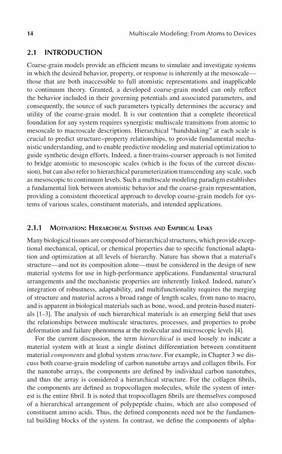
13

2 Coarse-Graining Parameterization and Multiscale Simulation of Hierarchical Systems. Part I: Theory and Model Formulation

Steve Cranford and Markus J. Buehler

contents

2.1 Introduction .................................................................................................... 142.1.1 Motivation: Hierarchical Systems and Empirical Links .................... 142.1.2 Diversity of Systems and Applications: Need for a System-

Dependent Approach .......................................................................... 162.1.3 Alternative Coarse-Graining Advantages: Pragmatic System

Simplification ...................................................................................... 172.1.4 When to Coarse-Grain: Appropriate Systems and

Considerations .................................................................................... 192.2 Examples of Coarse-Graining Methods ......................................................... 19

2.2.1 Elastic Network Models ...................................................................... 212.2.2 Two Potential Freely Jointed Chain Polymer Models ........................222.2.3 Generalization of Interactions: The MARTINI Force Field .............232.2.4 Universal Framework, Diverse Applications .....................................26

2.3 Model Formulation .........................................................................................262.3.1 Characterize the System: Coarse-Grain Potential Type and

Quantity ..............................................................................................272.3.2 Full Atomistic Test Suite ....................................................................282.3.3 Fitting Coarse-Grain Potentials ..........................................................282.3.4 Direct Energy Equivalence .................................................................28

2.3.4.1 Consistent Mechanical Behavior .........................................292.3.5 Validation ............................................................................................30

2.4 Summary and Conclusions .............................................................................30Acknowledgments .................................................................................................... 32References ................................................................................................................ 32

14 Multiscale Modeling: From Atoms to Devices

2.1 IntroductIon

Coarse-grain models provide an efficient means to simulate and investigate systems in which the desired behavior, property, or response is inherently at the mesoscale—those that are both inaccessible to full atomistic representations and inapplicable to continuum theory. Granted, a developed coarse-grain model can only reflect the behavior included in their governing potentials and associated parameters, and consequently, the source of such parameters typically determines the accuracy and utility of the coarse-grain model. It is our contention that a complete theoretical foundation for any system requires synergistic multiscale transitions from atomic to mesoscale to macroscale descriptions. Hierarchical “handshaking” at each scale is crucial to predict structure–property relationships, to provide fundamental mecha-nistic understanding, and to enable predictive modeling and material optimization to guide synthetic design efforts. Indeed, a finer-trains-coarser approach is not limited to bridge atomistic to mesoscopic scales (which is the focus of the current discus-sion), but can also refer to hierarchical parameterization transcending any scale, such as mesoscopic to continuum levels. Such a multiscale modeling paradigm establishes a fundamental link between atomistic behavior and the coarse-grain representation, providing a consistent theoretical approach to develop coarse-grain models for sys-tems of various scales, constituent materials, and intended applications.

2.1.1 Motivation: hierarChiCal systeMs and eMPiriCal links

Many biological tissues are composed of hierarchical structures, which provide excep-tional mechanical, optical, or chemical properties due to specific functional adapta-tion and optimization at all levels of hierarchy. Nature has shown that a material’s structure—and not its composition alone—must be considered in the design of new material systems for use in high-performance applications. Fundamental structural arrangements and the mechanistic properties are inherently linked. Indeed, nature’s integration of robustness, adaptability, and multifunctionality requires the merging of structure and material across a broad range of length scales, from nano to macro, and is apparent in biological materials such as bone, wood, and protein-based materi-als [1–3]. The analysis of such hierarchical materials is an emerging field that uses the relationships between multiscale structures, processes, and properties to probe deformation and failure phenomena at the molecular and microscopic levels [4].

For the current discussion, the term hierarchical is used loosely to indicate a material system with at least a single distinct differentiation between constituent material components and global system structure. For example, in Chapter 3 we dis-cuss both coarse-grain modeling of carbon nanotube arrays and collagen fibrils. For the nanotube arrays, the components are defined by individual carbon nanotubes, and thus the array is considered a hierarchical structure. For the collagen fibrils, the components are defined as tropocollagen molecules, while the system of inter-est is the entire fibril. It is noted that tropocollagen fibrils are themselves composed of a hierarchical arrangement of polypeptide chains, which are also composed of constituent amino acids. Thus, the defined components need not be the fundamen-tal building blocks of the system. In contrast, we define the components of alpha-

Coarse-Graining Parameterization and Multiscale Simulation 15

helical proteins (see case study in Chapter 3) as a single-protein convolution, while the system is characterized by the entire protein, recognizing the hierarchical effects of single molecular conformations. The coarse-graining procedures discussed here focus on constituent materials that can be modeled by full atomistic techniques using classical molecular dynamics, while the system structure (and relevant behaviors) requires a fully informed coarse-grain representation. The atomistic model provides the underlying physics to the coarse-grain potentials, allowing the investigation of structure–property functions at the required length scale.

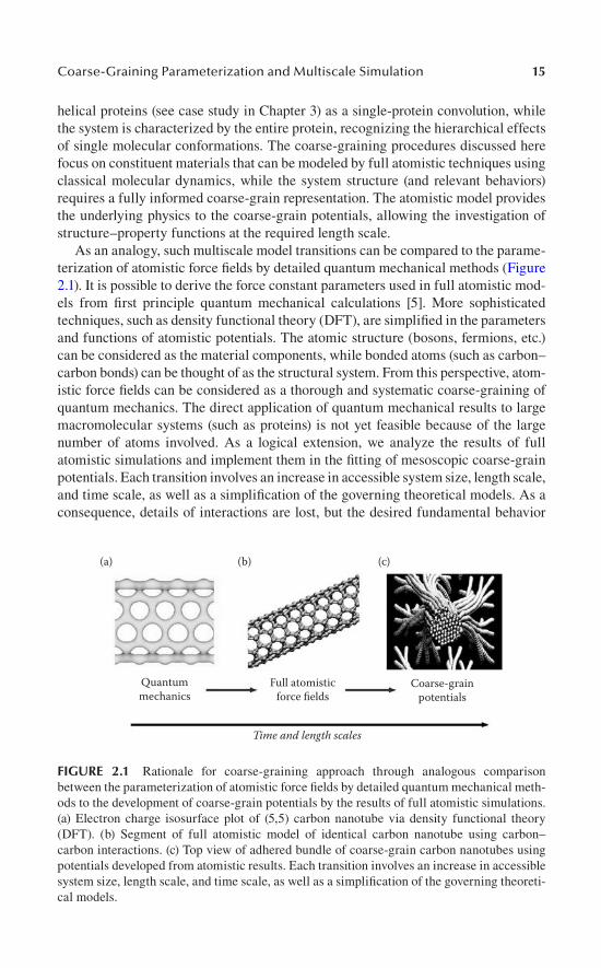
As an analogy, such multiscale model transitions can be compared to the parame-terization of atomistic force fields by detailed quantum mechanical methods (Figure 2.1). It is possible to derive the force constant parameters used in full atomistic mod-els from first principle quantum mechanical calculations [5]. More sophisticated techniques, such as density functional theory (DFT), are simplified in the parameters and functions of atomistic potentials. The atomic structure (bosons, fermions, etc.) can be considered as the material components, while bonded atoms (such as carbon–carbon bonds) can be thought of as the structural system. From this perspective, atom-istic force fields can be considered as a thorough and systematic coarse-graining of quantum mechanics. The direct application of quantum mechanical results to large macromolecular systems (such as proteins) is not yet feasible because of the large number of atoms involved. As a logical extension, we analyze the results of full atomistic simulations and implement them in the fitting of mesoscopic coarse-grain potentials. Each transition involves an increase in accessible system size, length scale, and time scale, as well as a simplification of the governing theoretical models. As a consequence, details of interactions are lost, but the desired fundamental behavior

(a)

Quantummechanics

Full atomisticforce fields

Time and length scales

Coarse-grainpotentials

(b) (c)

FIgure 2.1 Rationale for coarse-graining approach through analogous comparison between the parameterization of atomistic force fields by detailed quantum mechanical meth-ods to the development of coarse-grain potentials by the results of full atomistic simulations. (a) Electron charge isosurface plot of (5,5) carbon nanotube via density functional theory (DFT). (b) Segment of full atomistic model of identical carbon nanotube using carbon– carbon interactions. (c) Top view of adhered bundle of coarse-grain carbon nanotubes using potentials developed from atomistic results. Each transition involves an increase in accessible system size, length scale, and time scale, as well as a simplification of the governing theoreti-cal models.


is maintained. It is noted that this “desired fundamental behavior” is dependent on the system application, and can include mechanistic behaviors, thermal or electrical properties, molecular interactions, equilibrium configurations, etc. To illustrate, an atomistic representation of carbon bonding can include terms for atom separation, angle, and bond order (such as CHARMM [6]- or AMBER [6,7]-type force fields), but lacks any description of electron structure, band gaps, or transition states found in quantum mechanical approaches such as DFT. However, the atomistic model main-tains the accurate behavior of the individual carbon atoms and neglecting the effects of electrons is deemed a necessary simplification. Likewise, the coarse- graining of a carbon nanotube integrates the effects of multiple carbon bonds into a single potential. The exact distribution of carbon interactions is lost, but the behavior of the molecular structure is maintained.

The development of coarse-grain models allows the simulation of events on physi-cal time and size scales, leading to a range of possible advances in nanoscale design and molecular engineering in a completely integrated bottom-up approach. A coarse-graining approach is intended to develop tools to investigate material properties and underlying mechanical behavior typically required for material design that system-atically integrates characteristic chemical responses. However, it is emphasized that the intention is not to circumvent the need for full atomistic simulations—in con-trast, coarse-graining requires accurate full atomistic representations to acquire the necessary potential parameters. The finer-trains-coarser procedure described here is an attempt to reconcile first principles derivations with hierarchical multiscale techniques by using atomistic theory with molecular dynamics simulations in lieu of empirical observations in a unified and systematic approach.

2.1.2 diversity oF systeMs and aPPliCations: need For a systeM-dePendent aPProaCh

Atomistic force fields, which must encompass atom-atom bonds and interactions, can be developed in a general formulation due to the common molecular compo-nents. For example, the behavior of carbon–carbon bonds in a carbon nanotube is similar to the alpha-carbon backbone of a protein sequence in terms of strength and bond length. A thoroughly developed atomistic force field is capable of representing a vast assortment of molecular systems. Coarse-grained potentials, conversely, are usually developed to represent a particular system, and consequently feature unique idiosyncrasies in construction and behavior. Accordingly, differences in system com-plexity and goals of modeling lead to difficulties in developing a universal method for coarse-graining.

Attempts to avoid this system-dependent approach (i.e., generalized coarse-graining frameworks) can potentially result in a complex coarse-grain description to account for the multitude of molecular interactions a general description must encom-pass. The introduction of many potentials and parameters essentially mimic the function and form of full atomistic force fields, albeit at a coarse-grain scale. Other generalized frameworks attempt to simplify the description of molecular interactions as much as possible. For example the MARTINI force field [8] has been successful


in the intent of efficiently modeling larger systems, and warrants further discussion (see Section 2.3). To capture fundamental interactions, general coarse-grain poten-tials developed for application to multiple systems are limited to few atom mappings (i.e., two-, four-, and six-bead models) and are beneficial and appropriate for systems where the interactions are still at the atomistic scale (i.e., proteins, polymers, etc.).

It is apparent that different material systems can be characterized by mechanical properties at the atomistic to microscale, requiring a more general coarse-graining approach to model the intended structure–property behavior. It is our proposition that a hierarchical multiscale system requires a system-dependent approach to coarse-graining. Accurate system representation is maintained at a cost of coarse-grain potential versatility. By applying a system-dependent finer-trains-coarser ap proach, a variety of systems can be coarse-grained and modeled for different purposes, tran-scending different scales and functionalities. Such derived coarse-grain potentials are not meant to be universally applicable, but provide a means to investigate a spe-cific system under specific conditions.

2.1.3 alternative Coarse-GraininG advantaGes: PraGMatiC systeM siMPliFiCation

A commonly stated motivation and presumed primary benefit for the development of coarse-grain potentials and models is to allow the simulation of larger systems at longer time scales. Indeed, the reduction of system degrees-of-freedom and the smoother potentials implemented allow larger time-step increments (and thus time scales) and each element is typically an order of magnitude or more larger in length scale. Additionally, cheaper potential calculations (in terms of computational effi-ciency) can be exploited to either increase the number of coarse-grain elements (thus representing even larger systems) or simulate a relatively small system over more integration steps (further extending accessible time scales). Such benefits are inher-ent to any coarse-grain representation, and can serve as a de facto definition of the coarse-graining approach.

Nevertheless, a pragmatic approach of system simplification is found in many engineering disciplines. Complex electronic components are designed based on sim-plified models of circuits, with element behavior defined by such general proper-ties as current, voltage, and resistance. Robust building structures are analyzed via notions of beam deflections and beam-column joint rotations, among other simpli-fying assumptions. In both cases, more detailed system representations are known and can be implemented (e.g., implementation of temperature and material effects in a transistor, or a detailed frame analysis including stress concentrations in bolts or welds). It is apparent that such additions result in a more accurate representa-tion of the modeled system, but also serve to increase the computational expense of analysis as well as introduce a more sophisticated theoretical framework (which subsequently requires a more detailed set of material and model parameters). Rarely, however, is the use of simplified and computationally efficient models justified by inaccessible time and length scales of the more detailed description. Such models are applied for analysis in lieu of a more detailed description because they provide


an accurate representation of the system-level behavior and response with confidence in the properties of the model components.

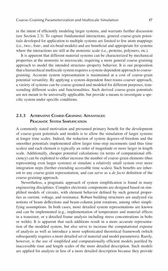
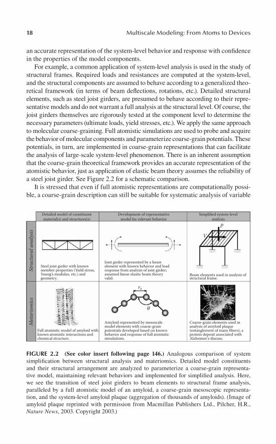
For example, a common application of system-level analysis is used in the study of structural frames. Required loads and resistances are computed at the system-level, and the structural components are assumed to behave according to a generalized theo-retical framework (in terms of beam deflections, rotations, etc.). Detailed structural elements, such as steel joist girders, are presumed to behave according to their repre-sentative models and do not warrant a full analysis at the structural level. Of course, the joist girders themselves are rigorously tested at the component level to determine the necessary parameters (ultimate loads, yield stresses, etc.). We apply the same approach to molecular coarse-graining. Full atomistic simulations are used to probe and acquire the behavior of molecular components and parameterize coarse-grain potentials. These potentials, in turn, are implemented in coarse-grain representations that can facilitate the analysis of large-scale system-level phenomenon. There is an inherent assumption that the coarse-grain theoretical framework provides an accurate representation of the atomistic behavior, just as application of elastic beam theory assumes the reliability of a steel joist girder. See Figure 2.2 for a schematic comparison.

It is stressed that even if full atomistic representations are computationally possi-ble, a coarse-grain description can still be suitable for systematic analysis of variable

θ

r0

Stru

ctur

al a

naly

sisM

etar

iom

ics

Detailed model of constituentmaterial(s) and structures(s)

Development of representativemodel for relevant behavior

Simplified system-levelanalysis

Beam elements used in analysis ofstructural frame.

V

P

Joist girder represented by a beamelement with known behavior and loadresponse from analysis of joist girder;assumed linear elastic beam theoryvalid.

Steel joist girder with knownmember properties (Yield stress,Young’s modulus, etc.) andgeometry.

Amyloid represented by mesoscalemodel elements with coarse-grainpotentials developed based on knownbehavior and response of full atomisticsimulations.

Coarse-grain elements used inanalysis of amyloid plaque(entanglement of many fibers), aprotein deposit associated withAlzheimer’s disease.

Full atomistic model of amyloid withknown atomistic interactions andchemical structure.

FIgure 2.2 (See color insert following page 146.) Analogous comparison of system simplification between structural analysis and materiomics. Detailed model constituents and their structural arrangement are analyzed to parameterize a coarse-grain representa-tive model, maintaining relevant behaviors and implemented for simplified analysis. Here, we see the transition of steel joist girders to beam elements to structural frame analysis, paralleled by a full atomistic model of an amyloid, a coarse-grain mesoscopic representa-tion, and the system-level amyloid plaque (aggregation of thousands of amyloids). (Image of amyloid plaque reprinted with permission from Macmillan Publishers Ltd., Pilcher, H.R., Nature News, 2003. Copyright 2003.)


system configurations, which requires a large number of simulations. We offer an alternative motivation for a coarse-graining approach complementary to extension of accessible time and length scales, where the catalyst for coarse-grain potential development is not the extension of traditional molecular dynamics, but to provide an accurate and reliable method for system-level analysis and probe the mechani-cal response and structure–property relation for hierarchical systems. Furthermore, mesoscopic models provide simple and efficient modeling techniques for experimen-talists, allowing a more direct comparison between simulation and a vast variety of experimental techniques, without requiring specialized molecular dynamics tools such as specialized computer clusters with complex software.

2.1.4 When to Coarse-Grain: aPProPriate systeMs and Considerations

It is emphasized that not all systems will benefit from a coarse-grain representa-tion and prudent consideration must be given regarding the system characterization and intent of the simulations. For some systems, complex behaviors may require full atomistic representation, or material inhomogeneities may not be able to be described by coarse-grain elements. Such systems may benefit and indeed require full atomistic representations. Typical motivations for a coarse-graining approach include:

1. Inaccessible time scale for phenomenon or behavior via full atomistic representation

2. Inaccessible length scale for phenomenon or behavior via full atomistic representation

3. Focus on global system properties and/or mechanical behavior rather than on molecular structure and/or chemical interactions

4. Desire for a direct simplified analysis of simulation results and system behavior

In addition to these motivating factors, some systems are more conducive to coarse-graining due to chemical composure and/or structural arrangement. Coarse-grain models are easily adapted for atomistically homogenous systems, consisting of repetitive structures such as carbon nanotubes (with a uniform cylindrical nanostruc-ture). By extension, atomistically heterogeneous materials, such as protein-based materials, are applicable to coarse-graining if they are mesoscopically homogeneous, where the local effects of distinct amino acids (or other molecular inhomogeneities) produce similar global behaviors and are deemed negligible. Other system properties to consider include the discretization or material units and/or mechanical behavior, with a logical correlation to coarse-grain elements, and any hierarchical structures in which the intended structure–property relation is to be investigated.

2.2 exaMples oF coarse-graInIng Methods

In the past decade, various simple models have been used to describe the large-scale motions of complex molecular structures where more detailed classical


phenomenological potentials [6,7] involving all atoms cannot be used because of the restrictions on the amount of time that can be covered in computer simulations. The reader is referred to recent reviews for a more thorough discussion of techniques and applications [9–12].

Single-bead models are the most direct approach taken for studying macromol-ecules. The term single bead derives from the idea of using single beads, that is, point masses, for describing a functional group, such as single amino acids, in a mac-romolecular structure. The elastic network model (ENM) [13], Gaussian network model [14], and GO model [15] are well-known examples that are based on such bead model approximations. These models treat each amino acid as a single bead located at the Cα position, with mass equal to the mass of the amino acid. The beads are connected via harmonic bonding potentials, which represent the covalently bonded protein backbone. Elastic network models have been used to study the properties of coarse-grained models of proteins and larger biomolecular complexes, focusing on the structural fluctuations about a prescribed equilibrium configuration, such as normal vibrational modes, and are discussed further in Section 2.2.1.

In GO-like models, an additional Lennard–Jones-based term is included in the potential to describe short-range nonbonded interactions between atoms within a finite cutoff separation. Despite their simplicity, these models have been extremely successful in explaining thermal fluctuations of proteins [11] and have also been implemented to model the unfolding problem to elucidate atomic-level details of deformation and rupture that complement experimental results [16–18]. A more recent direction is coupling of ENM models with a finite element-type framework for mechanistic studies of protein structures and assemblies [19].

Using more than one bead per amino acid provides a more sophisticated descrip-tion of protein molecules. In the simplest case, the addition of another bead can be used to describe specific side-chain interactions in proteins [20]. Higher-level models (e.g., four- to six-bead descriptions) capture more details by explicit or united atom description for backbone carbon atoms, side chains, and carboxyl and amino groups of amino acids [21,22]. Coarser-level multiscale modeling methods similar to those presented here have been reported more recently, applied to model biomolecular systems at larger time and length scales. These models typically employ super-atom descriptions that treat clusters of amino acids as beads. In such models, the elasticity of a polypeptide chain is captured by simple harmonic or anharmonic (nonlinear) bond and angle terms. These methods are computationally quite efficient and cap-ture shape-dependent mechanical phenomena in large biomolecular structures [23], and can also be applied to collagen fibrils in connective tissue [24] as well as min-eralized composites such as nascent bone [25]. The development of the coarse-grain model for collagen will be discussed further as a case study in Chapter 3.

We proceed to provide a brief discussion of some of the aforementioned approaches implemented for coarse-grain potentials as an overview of other methods. The fol-lowing discussion is not intended to include all the intricacies and details of the development and application of each method, but merely to provide examples of various types of coarse-graining procedures and the progression of adding more complexity to the coarse-grain representation.


2.2.1 elastiC netWork Models

In the simplest form, a coarse-grain model can be defined by a single potential for all beads. For example, the aforementioned ENMs can be thought of as a single pair potential between neighbor atoms, such that:

E E rCG ENM ENM ( )= = ∑φ , (2.1)

where

φENM ( )r K r rr= −( )1

2 0

2

(2.2)

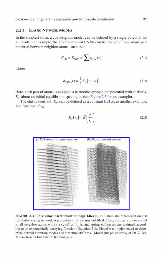
Here, each pair of atoms is assigned a harmonic spring bond potential with stiffness, Kr , about an initial equilibrium spacing, r0 (see Figure 2.3 for an example).

The elastic constant, Kr , can be defined as a constant [13] or, as another example, as a function of r0:

K r K

rrr 0

0( ) =

(2.3)

(a) Full atomistic representation (b) Elastic network model

FIgure 2.3 (See color insert following page 146.) (a) Full atomistic representation and (b) elastic spring network representation of an amyloid fibril. Here, springs are connected to all neighbor atoms within a cutoff of 10 Å, and spring stiffnesses are assigned accord-ing to an exponentially decaying function (Equation 2.4). Model was implemented to deter-mine normal vibration modes and structure stiffness. (Model images courtesy of Dr. Z. Xu, Massachusetts Institute of Technology.)

http://www.crcnetbase.com/action/showImage?doi=10.1201/b10454-3&iName=master.img-002.jpg&w=240&h=180


K r Krrr 00

2

( ) = −

exp (2.4)

Equation 2.3 scales the mean value of the elastic constant, K , with the initial bond length, r0, such that K r Kr ( ) = . If the ENM is representative of a solid or continuous media, this method treats all elastic elements as if they had the same cross-sectional area, A, and a constant Young’s modulus, E, such that the quantity (EA/r0) is the same for all elements in the network [26]. The second method subjects the elastic constant to an exponentially decaying function with respect to a mean bond distance (r ). Such a formulation of Kr can represent weak interactions of atoms at a distance (such as van der Waals interactions) and provide a more complex description of inter-actions [27,28].

Such ENMs fall into two broad classes, those with Hookean springs that describe the rigidity of the macromolecule [13], and those describing the connectivity of the macromolecule [29]. For illustrative purposes, we limit our discussion to scalar spring constants and forces along the vector between two atoms, but also note that more complex model representations introducing directionality and anisotropy can be formulated [30]. As such, even a single potential description can become increas-ingly sophisticated as applications attempt to probe complex molecular deformations such as protein residue fluctuations [31] and equilibrium state transitions [32,33].

2.2.2 tWo Potential Freely Jointed Chain PolyMer Models

Although useful in the application of normal mode analysis of single protein macro-molecules, ENM techniques lack the description necessary for intermolecular inter-actions and large deformation from equilibrium conditions. The subsequent step in coarse-grain model development is the combination of two simple potentials to represent the intermolecular and intramolecular interactions of individual macro-molecules. Polymer systems are frequently represented by two such coarse-grain potentials, which encompass intramolecular (bonded) interactions and intermolecu-lar (nonbonded) interactions, respectively, in a freely jointed chain (FJC) representa-tion (no angular constraints) or:

E E E r rCG bonded nonbonded FENE WCA( ) ( )= + = +∑ ∑φ φ (2.5)

For bonded beads, a finitely extensible nonlinear elastic (FENE) potential [34–36] is implemented to maintain distance between connected beads and prevent polymer chains from crossing each other:

φFENE lnr krrr

r r( ) = − −

<12

102

0

2

0for , (2.6)

ϕFENE(r) = ∞ for r ≥ r0


The Weeks–Chandler–Anderson (WCA) potential [37,38] is the Lennard–Jones 12:6 potential truncated at the position of the minimum and shifted to eliminate discontinuity:

φ εσ σ

σWCA ( )rr r

r=

−

<4 212 6

6for , (2.7)

φ

σWCA ( )rr= ≥0 26for

The WCA potential results in a purely repulsive potential. The combination of the FENE attractive potential with the WCA repulsive interaction creates a potential well for the flexible bonds that can maintain the topology of the molecule [39]. Such models can successfully represent stretching, orientation, and deformation of poly-mer chains and simple biomolecules.

Due to the inherent flexibility of the freely jointed chains, this coarse-graining approach is particularly suited for systems defined by long-chain polymers with relatively short persistence lengths, or systems that are entropically driven. As such, example applications include the investigation of viscoelastic behavior of polymer melts [40], stretching of polymers in flow [41], and other rheological properties [42,43]. More complex formulations use the combination of FENE and WCA poten-tials to define the coarse-grain model, and add additional potentials for a more robust description of the system, such as the introduction of angular terms (for stiffness) and Coulombic terms (for electrostatic interactions) to model complex macromol-ecules such as DNA [44].

2.2.3 Generalization oF interaCtions: the Martini ForCe Field

The lack of intermolecular interaction characterization in the previous coarse- graining approaches required a more complex formulation—one that maintained a definitive structure of the macromolecule, as well as integrated the interactions between macromolecules. The development of the MARTINI force field attempted to provide a general coarse-grain model that could be efficiently adapted for a mul-titude of biological systems by taking advantage of the fact that the majority of bio-logical molecules (such as protein structures and lipids) are composed of the same categories of functional groups at the atomistic level [8,45,46]. Such approaches were previously implemented with various degrees of complexity for application to specific systems, integrating multiple beads per functional group, or more complex parameter formulations (see Marrink et al. [45] for a discussion and Shelley et al. [47,48] as examples). Essentially, by coarse-graining the functional groups, mole-cules with different architectures can be easily built and simulated. The aim of the MARTINI force field was to retain the chemical nature of the molecular components while defining as few bead types as possible. The applied philosophy was to avoid a focus on the reproduction of structural details for a particular system, but rather


aim for a broad range of applications without the need to reparameterize the model each time. As a result, there is a slight trade-off between accuracy and applicability, with many different biological systems able to be modeled. Only four interaction types are considered—polar, nonpolar, apolar, and charged—and subtypes of these interactions are used to define hydrogen-bonding characteristics (see Figure 2.4 for coarse-grain representations of amino acids).

The MARTINI force field can be represented by

E E E E rMARTINI bond angle nonbonded T ( ) ( )= + + = + +∑ ∑φ φ θθ φφLJ ( )r∑ , (2.8)

where harmonic potentials are implemented for the bonded and angle potentials, or:

φT T( )r k r r= −( )1

2 0

2 (2.9)

φ θ θθ θ( ) cos cosr k= −( )1

2 0

2 (2.10)

The harmonic potentials are parameterized by constants (kT, r0, kθ, and θ0) common to all bead-types. Such an approach increases the general applicability and versatil-ity of the force field. Nonbonded interactions between interaction sites i and j are described by the Lennard–Jones 12:6 potential:

Ala

Arg

Asn

Asp

Cys

Gln

Glu

Gly

His

Ile

Leu

Lys

Met

Phe

Pro

Ser

Thr

Trp

Tyr

Val

apolar polarintermediate charged

FIgure 2.4 (See color insert following page 146.) Coarse-grain representations of all amino acid types for MARTINI force field formulation for proteins. Different colors repre-sent different particle types consisting of four main types of interaction sites: polar, nonpolar, apolar, and charged. (Reprinted with permission from Monticelli, L., et al., J. Chem. Theory Comput., 4, 819–834, 2008. Copyright 2008 American Chemical Society.)


φ εσ σ

LJ ( )rr rijij ij=

−

4

12 6

, (2.11)

with σij representing the effective minimum distance between two particles, and εij the strength of their interaction. The uniqueness of the MARTINI force field param-eterization is the arrangement of both σij and εij into distinct subsets of interaction groups.

The major advantage of the MARTINI force field is the simplicity and versa-tility of the parameterization—many proteins, lipids, and molecules can be built using the same set of coarse-grain building blocks. However, these MARTINI-type formulations restrict the coarse-graining to distinct functional groups to accurately maintain atomistic interactions while increasing computational efficiency. The obvi-ous disadvantage of such approaches lies in the restriction of the coarse-graining scale. For example, on average, each bead of the MARTINI model has the volume of four water molecules. As a result, the time and length scales of MARTINI and MARTINI-type simulations are still limited, albeit much more efficient than full atomistic approaches. Again, prudence is required in selecting the level of detail of the coarse-grain representation.

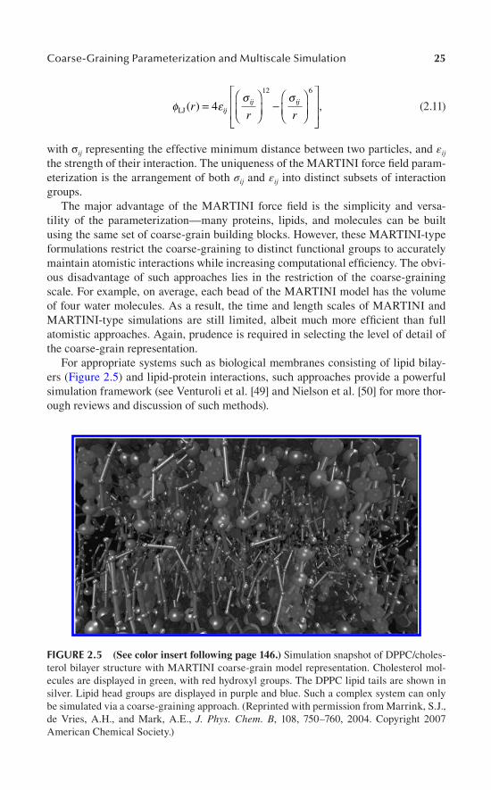
For appropriate systems such as biological membranes consisting of lipid bilay-ers (Figure 2.5) and lipid-protein interactions, such approaches provide a powerful simulation framework (see Venturoli et al. [49] and Nielson et al. [50] for more thor-ough reviews and discussion of such methods).

FIgure 2.5 (See color insert following page 146.) Simulation snapshot of DPPC/choles-terol bilayer structure with MARTINI coarse-grain model representation. Cholesterol mol-ecules are displayed in green, with red hydroxyl groups. The DPPC lipid tails are shown in silver. Lipid head groups are displayed in purple and blue. Such a complex system can only be simulated via a coarse-graining approach. (Reprinted with permission from Marrink, S.J., de Vries, A.H., and Mark, A.E., J. Phys. Chem. B, 108, 750–760, 2004. Copyright 2007 American Chemical Society.)

http://www.crcnetbase.com/action/showImage?doi=10.1201/b10454-3&iName=master.img-004.jpg&w=288&h=164


2.2.4 universal FraMeWork, diverse aPPliCations

The aforementioned coarse-graining techniques, ENM models, FJC representations, and MARTINI-type formulations have been successful in their own applications. ENMs reflect the atomistic structure, FJC representations can accurately reproduce polymer flow and rheological properties, while MARTINI-type models accurately capture the interactions of functional groups for applications in assembly. However, such techniques focus on molecular geometry and interactions rather than reflect accurate mechanical properties and response. We predict that the investigation of the mechanical behavior of hierarchical systems requires a system-dependent param-eterization of coarse-grain potentials, with a focus on maintaining both molecular interactions and molecular mechanics. Thus, we introduce a universal framework through a finer-trains-coarser multiscale paradigm, which effectively defines coarse-grain potentials via the response of full atomistic simulations, while introducing relevant mechanical properties at the mesoscopic scale. The approach is unique in its ability to transcend multiple scales, enabling the investigation of a broad regime of systems from protein-based materials to synthetic composite structures, while emphasizing a theoretical foundation on full atomistic investigations and asserting energetic equivalence and consistent mechanical behavior between all levels of mod-eling. The result is a set of problem-specific coarse-grain representations with diverse applications. The discussion in Section 2.3 presents guiding principles behind model formulation.

2.3 Model ForMulatIon

From the previous discussion, it is apparent that a universal, stepwise procedure for coarse-graining a system is limited by the inherent simplifications and intent of the coarse-grain representation. A model developed to investigate arrays of carbon nanotubes (see Chapter 3, Case Study I) will differ from a model developed for the simulation of alpha-helix unfolding (see Chapter 3, Case Study II), even though the coarse-grain elements and potentials are similar. The coarse-graining of a particular system can be characterized by trial-and-error and subjective omissions or inclu-sions of pertinent behaviors, and as such considered just as much an art as a science. Careful consideration must be taken for the intended application and purpose of the coarse-grain model. Indeed, such a judicious approach is the motivation for a finer-trains-coarser approach. A deliberate focus on the atomistic behavior to characterize the coarse-grain model not only provides a complete “bottom-up” theoretical basis for a material system, but also assists in the formulation of the coarse-grain model by delineating relevant behavior and interactions. Nevertheless, although we con-tend that a step-by-step coarse-graining “recipe” is problematic, we can outline the “ingredients” in a general, coarse-graining framework:

1. Potentials required to define and characterize the mesoscale system 2. Full atomistic “test suite” applied to determine required coarse-grain poten-

tial parameters


3. Fitting of atomistic results to coarse-grain potential parameters via energy equivalence and consistent mechanical behavior

4. Validation of coarse-grain model with full atomistic and/or empirical results

We proceed to discuss each in detail.

2.3.1 CharaCterize the systeM: Coarse-Grain Potential tyPe and quantity

The first step in the development of a coarse-grain model is to determine the neces-sary potentials to characterize the system. In general, we define the total energy of a coarse-grain system as the sum of these potentials:

E ESystem CG CG= = ∑φ , (2.12)

where ϕCG is the defined coarse-grain potentials. Although a simple statement, it is not trivial in implementation. Indeed, the type of developed potentials can serve to both broaden and restrict the applications of the model. Specifically, the coarse-grain potentials must be complex enough to represent the molecule in the intended meso-scopic simulation. One must consider whether provisions are necessary for fracture, intermolecular interactions, plasticity, formation of secondary structures, or a host of other molecular behaviors depending on the intent of the investigation. It is again stressed that a coarse-grain model for a system is not universal. The goal is to utilize the fewest and simplest potentials as possible that represent the system structure(s), mechanical properties, and interactions. Such an approach can be facilitated by the utilization of harmonic spring potentials to reflect mechanical response, where

φ ψ ψ ψi ik( ) = −( )1

2 0

2 (2.13)

Here, ki refers to a harmonic spring stiffness while ψ typically refers to either an interatomic distance, r, or an angle, θ, for stretching and bending deformations, respectively. The harmonic spring potential results in a linear relationship between force and deformation, allowing efficient computation of interactions. Indeed, more complex nonlinear behavior can be approximated by combinations of linear func-tions (such as bilinear or trilinear formulations) to maintain computational efficiency in lieu of the introduction of more complex potentials (such an approach is discussed further in the ensuing chapter). A possible deficiency of harmonic potentials is the continuous increase in force with deformation. Systems subject to large deforma-tions will subsequently deviate from true behavior, and thus, without provisions such as a potential cutoff, the use of the harmonic potential should be limited to small deformation. Selection of the harmonic spring potential can also be affected by the atomistic response by which it is parameterized. For example, a linear elastic strain


response can be sufficiently modeled by harmonic spring potentials, albeit limited to small deformation.

2.3.2 Full atoMistiC test suite

The finer-trains-coarser approach necessitates the parameterization of coarse-grain potentials from full atomistic results. An atomistic test suite is thus developed to obtain the necessary mechanical response and molecular interactions to be inte-grated into coarse-grain potentials. Typically, a relatively simple atomistic simula-tion is applied to isolate a single molecular behavior, mimicking simple material specimen tests. For example, uniaxial stretching can be applied to obtain the force- displacement or stress-strain response of a macromolecule, allowing the calcula-tion of Young’s modulus, and the parameterization of coarse-grain bond strength. Further, a three-point bending test can be utilized to determine the bending stiffness of a molecule, thereby allowing the parameterization of the coarse-grain bending potential. For molecular interactions, pairs of molecules are simulated to deter-mine relative adhesion. In essence, a single atomistic investigation is implemented to characterize a single coarse-grain potential, ensuring accurate representation of each behavior. The number of required tests depends on the number of coarse-grain potentials (and associated parameters) implemented to describe the system.

2.3.3 FittinG Coarse-Grain Potentials

The fundamental principle underlying the parameterization of coarse-grain poten-tials is the assertion of energy conservation. Energy equivalence is imposed between potential energy functions and relevant atomistic energy results. The basis of the formulation of the energy functions, either through elastic strain energy, deformation energy, adhesion energy, or other techniques, essentially defines the accuracy and behavior of the representative coarse-grain system. Two such approaches of energy conservation warrant separate discussions: (1) the application of direct energy equiv-alence between atomistic and coarse-grain representations and (2) the assertion of energy conservation via consistent mechanical behavior.

2.3.4 direCt enerGy equivalenCe

Nonbonded interactions representing macromolecular adhesion, attraction, or repul-sion innately have no mechanical property analogue for parameterization. For such energetic potentials as the Lennard–Jones 12:6 function, or Coulombic interac-tions, the coarse-grain equivalent is extracted directly from the energetic results of a full atomistic representation. Potential energy as a function of separation can be derived between individual macromolecules. The coarse-grain potential can then be expressed as

φ ω φCG

atoms

( )R rij ij ij= ( )∑ , (2.14)


where ϕCG is the coarse-grain potential, R is the macromolecular separation, and

ω φij ij ijr( )∑atoms

is a weighted summation of the full atomistic potentials, ϕij. This is

essentially how coarse-grain potentials are developed for a small number of atoms per superatom (such as MARTINI-type force fields), where the superposition of mul-tibody effects is apparent in the mapping. The relation becomes more complex as the number of incorporated/mapped atoms increase, requiring explicit atomistic simula-tion of the desired macromolecules. The above relation should not be thought of as a simple summation of potentials, or:

φ εσ σ

εCG-LJ ( )RR Rij ij

=

−

≠4 4

12 6

iijij

ij

ij

ijr r

σ σ

−

12 6

aatoms

∑ . (2.15)

The coarse-grain potential incorporates effects of the entire represented system (such as hydrophobic and other solvent effects, electrostatic interactions, hydrogen bonding between molecules, and/or entropic effects). We thereby introduce unknown weighting coefficients, ωij, in the summation of Equation 2.14. The complexity neces-sitates a full atomistic investigation to derive the effective coarse-grain potential parameters.

2.3.4.1 consistent Mechanical behaviorBonded and angle potentials effectively represent molecular mechanical behavior. As there can be many contributions to even simple mechanical processes (such as the breaking of hydrogen bonds or solvent friction during molecular stretching or bend-ing), we introduce conservation of energy for the relevant mechanical response (as opposed to the potential energy of direct energy equivalence) resulting in consistent mechanical behavior between full atomistic and coarse-grain representations. The approach is to apply energy equivalence between the coarse-grain potential and the observed strain or deformation energy of the full atomistic system:

ϕCG(ψ) = U(ψ), (2.16)

where ϕCG(ψ) is again the coarse-grain potential, and U(ψ) is the representative energy function for the mechanical response. It is an underlying assumption of the model that the response of the full atomistic system is accurately described by the energy function, U(ψ). The choice of the strain or deformation energy function is dependent on the system to be coarse-grained, and assumptions of elastic/plastic behavior, material isotropy, system failure such as yielding or fracture, etc. affect the definition (and interpretation) of atomistic results. As an example, for an elastic-isotropic material, we can define strain energy as

U V

V

( ) [ ][ ]dε σ ε= ∫12

. (2.17)


To equate with ϕCG(ψ), we must formulate U as a function of ψ. For axial stretching, this requires the formulation of strain as a function of bond length, ε(r), while for shearing this requires the formulation of strain as a function of shearing angle, ε(θ).

Individual parameterization of coarse-grain potentials via consistent mechanical behavior has an inherent limitation by the decoupling of mechanical behavior. To illustrate, as bond and angle coarse-grain potentials are independent under simula-tion, there is no coupling between stretching and bending of the molecule and effects such as twisting or torque are completely neglected. However, under full atomis-tic representations, such coupling can serve to increase stresses and induce failure. Ultimately, the model is tailored to the desired application, and systems with obvious or significant coupling effects should be avoided.

2.3.5 validation

Once the coarse-grain potentials are developed, validation of the coarse-grain model is a necessary step to assure an accurate representation. The primary basis for vali-dation is through a direct comparison to full atomistic simulations. Such an approach may seem counterintuitive, redundant, or self-serving as the coarse-grain potentials were developed from such simulation results. However, the test suites applied were intended to result in a single behavior/response for each coarse-grain potential. The full coarse-grain representation can possibly involve the interaction and/or coupling of individual potentials. The combination of two behaviors (bending and stretching, for example) must be explored to justify the coarse-grain model. Relatively simple validation simulations can be designed, combining multiple system behaviors, and a one-to-one comparison made between full atomistic and coarse-grain results.

Due to limitations of full atomistic simulations, such validation is restricted to component-level behavior in which the coarse-grain model is specifically developed to circumvent. If available, secondary support and model validation is found in exper-imental data. Experimental techniques such as nanoindentation or atomic or chemi-cal force microscopy (AFM/CFM) can directly probe materials at the mesoscale and determine system level characteristics and mechanical properties. The development of coarse-grain models is intended to elucidate such system-level behavior and thus correlation with experimental results is essential. Reciprocally, an accurate coarse-grain model can serve to validate and support experimental results.

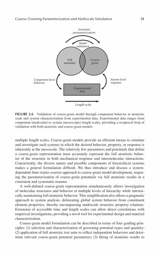
It is noted that advances in experimental techniques are continually probing smaller scales, reaching atomistic precision, and allowing single molecule investigations [such as optical tweezer methods, atomic force microscopy (AFM), etc.]. Such data can serve to reinforce both the full atomistic representation and the developed coarse-grain model, thereby increasing confidence in both representations and supporting the finer-trains-coarser approach. Figure 2.6 provides a schematic of the relationship between atomistic and coarse-grain representations with experimental data for model validation.

2.4 suMMary and conclusIons

The interplay between material properties and structural arrangement of hierar-chical systems provides unique and robust mechanical behavior that transcends


multiple length scales. Coarse-grain models provide an efficient means to simulate and investigate such systems in which the desired behavior, property, or response is inherently at the mesoscale. The relatively few parameters and potentials that define a coarse-grain representation must accurately represent the full atomistic behav-ior of the structure in both mechanical response and intermolecular interactions. Concurrently, the diverse nature and possible components of hierarchical systems makes a general formulation difficult. We thus introduce and discuss a system- dependent finer- trains-coarser approach to coarse-grain model development, requir-ing the parameterization of coarse-grain potentials via full atomistic results in a consistent and systematic manner.

A well-defined coarse-grain representation simultaneously allows investigation of molecular structures and behavior at multiple levels of hierarchy while intrinsi-cally maintaining full atomistic behavior. This simplification also allows a pragmatic approach to system analysis, delineating global system behavior from constituent element properties, thereby encompassing multiscale structure–property relations. Extension of accessible time and length scales can allow direct correlations with empirical investigations, providing a novel tool for experimental design and material characterization.

Coarse-grain model formulation can be described in terms of four guiding prin-ciples: (1) selection and characterization of governing potential types and quantity; (2) application of full atomistic test suite to reflect independent behaviors and deter-mine relevant coarse-grain potential parameters; (3) fitting of atomistic results to

Atomisticparameterization

Modelvalidation

Component levelbehavior

System levelresponse

Length scale

Experimentaldata

Coarsegrain

Fullatomistic

FIgure 2.6 Validation of coarse-grain model through component behavior at atomistic scale and system characterization from experimental data. Experimental data ranges from component (molecular) to system (mesoscopic) length scales, providing a reciprocal loop of validation with both atomistic and coarse-grain models.


necessary potential parameters via direct energy equivalence of conservation of energy through consistent mechanical behavior; and (4) validation of the developed model via comparison with full atomistic results (component-level) or correlation with empirical data (system-level).

acknowledgMents

This research was supported by the Army Research Office (W911NF-06-1-0291), the National Science Foundation (CAREER Grant CMMI-0642545 and MRSEC DMR-0819762), the Air Force Office of Scientific Research (FA9550-08-1-0321), the Office of Naval Research (N00014-08-1-00844), and the Defense Advanced Research Projects Agency (DARPA) (HR0011-08-1-0067). M. J. B. acknowledges support through the Esther and Harold E. Edgerton Career Development Professorship.

reFerences

1. Fratzl, P. and R. Weinkamer. 2007. Nature’s hierarchical materials. Progress in Materials Science. 52:1263–1334.

2. Buehler, M. J., S. Keten, and T. Ackbarow. 2008. Theoretical and computational hier-archical nanomechanics of protein materials: Deformation and fracture. Progress in Materials Science 53:1101–1241.

3. Espinosa, H. D., et al. 2009. Merger of structure and material in nacre and bone—Perspectives on de novo biomimetic materials. Progress in Materials Science 54:1059–1100.

4. Buehler, M. J. and Y. C. Yung. 2009. Deformation and failure of protein materials in physiologically extreme conditions and disease. Nature Materials 8(3):175–188.

5. Car, R. and M. Parrinello. 1985. Unified approach for molecular dynamics and density-functional theory. Physical Review Letters 55(22):2471–2474.

6. Brooks, B. R., et al. 1983. CHARMM: A program for macromolecular energy, minimi-zation, and dynamics calculations. Journal of Computational Chemistry 4(2):187–217.

7. Pearlman, D. A. et al. 1995. AMBER, a package of computer programs for applying molecular mechanics, normal mode analysis, molecular dynamics and free energy cal-culations to simulate the structural and energetic properties of molecules. Computer Physics Communications 91(1):1–41.

8. Marrink, S. J. et al. 2007. The MARTINI force field: Coarse Grained Model for Biomolecular Structures. Journal of Physical Chemistry B 111:7812–7824.

9. Tama, F. and C. L. Brooks, III. 2006. Symmetry, form, and shape: Guiding princi-ples for robustness in macromolecular machines. Annual Reviews in Biophysics and Biomolecular Structure 35:115–133.

10. Bahar, I. and A. J. Rader. 2005. Coarse-grain normal model analysis in structural biol-ogy. Current Opinion in Structural Biology 15:586–592.

11. Tozzini, V. 2005. Coarse-grained models for proteins. Current Opinion in Structural Biology 15:144–150.

12. Sherwood, P., B. R. Brooks, and M. S. P. Sansom. 2008. Multiscale methods for macro-molecular simulations. Current Opinion in Structural Biology 18:630–640.

13. Tirion, M. M. 1996. Large amplitude elastic motions in proteins from a single- parameter, atomic analysis. Physical Review Letters 77(9):1905–1908.

14. Haliloglu, T., I. Bahar, and B. Erman. 1997. Gaussian dynamcs of folded proteins. Physical Review Letters 79(16):3090–3093.


15. Hayward, S. and N. Go. 1995. Collective variable description of native protein dynam-ics. Annual Review of Physical Chemistry 46:223–250.

16. West, D. K. et al. 2006. Mechancial resistance of proteins explained using simple molec-ular models. Biophysical Journal 90(1):287–297.

17. Dietz, H. and M. Rief. 2008. Elastic bond network model for protein unfolding mechan-ics. Physical Review Letters 100:098101.

18. Sulkowska, J. I. and M. Cieplak. 2007. Mechanical stretching of proteins—a theoretical survey of the Protein Data Bank. Journal of Physics: Condensed Matter 19:283201.

19. Bathe, M. 2007. A finite element framework for computation of protein normal modes and mechanical response. Proteins: Structure, Functions, and Bioinformatics 70(4):1595–1609.

20. Bahar, I. and R. L. Jernigan. 1997. Inter-residue potentials in globular proteins and the dominance of highly specific hydrophilic interactions at close separation. Journal of Molecular Biology 266(1):195–214.

21. Nguyen, H. D. and C. K. Hall. 2004. Molecular dynamics simulations of spontane-ous fibril formation by random-coil peptides. Proceedings of the National Academy of Sciences 101(46):16180–16185.

22. Nguyen, H. D. and C. K. Hall. Spontaneous fibril formation by polyalanines: Discontinuous molecular dynamic simulations. Journal of the American Chemical Society 128(6):1890–1901.

23. Arkhipov, A., et al. 2006. Coarse-grained molecular dynamics simulations of a rotating bacterial flagellum. Biophysical Journal 91:4589–4597.

24. Buehler, M. J. 2006. Nature designs tough collagen: Explaining the nanostructure of col-lagen fibrils. Proceedings of the National Academy of Sciences 103(33):12285–12290.

25. Buehler, M. J. 2007. Molecular nanomechanics of nascent bone: Fibrillar toughening by mineralization. Nanotechnology 18:295102.

26. Hansen, J. C. et al. 1996. An elastic network model based on the structure of the red blood cell membrane skeleton. Biophysical Journal 70:146–166.

27. Hinsen, K. 1998. Analysis of domain motions by approximate normal mode calcula-tions. Proteins: Structure, Functions, and Genetics 33:417–429.

28. Hinsen, K., A. Thomas, and M. J. Field. 1999. Analysis of domain motions in large proteins. Proteins: Structure, Functions, and Genetics 34:369–382.

29. Bahar, I., A. R. Atilgan, and B. Erman. 1997. Direct evaluation of thermal fluctuations in proteins using a single-parameter harmonic potential. Folding and Design 2:173–181.

30. Atilgan, A. R. et al. 2001. Anisotropy of fluctuation dynamics of proteins with an elastic network model. Biophysical Journal 80:505–515.

31. Doruker, P., R. L. Jernigan, and I. Bahar. 2002. Dynamics of large proteins through hierarchical levels of coarse-grained structures. Journal of Computational Chemistry 23(1):119–127.

32. Navizet, I., R. Lavery, and R. L. Jernigan. 2004. Myosin flexibility: Structural domains and collective vibrations. Proteins: Structure, Functions, and Bioinformatics 54:384–393.

33. Zheng, W. and S. Doniach. 2003. A comparative study of motor-protein motions by using a simple elastic-network model. Proceedings of the National Academy of Sciences 100(23):13253–13258.

34. Warner, H. R., Jr. 1972. Kinetic theory and rheology of dilute suspensions of finitely extendible dumbells. Industrial and Engineering Chemistry Fundamentals 11(3):379–387.

35. Grest, G. S. and K. Kremer. 1986. Molecular dynamics simulation for polymers in the presence of a heat bath. Physical Review A 33(5):3628–3631.

36. Koplik, J. and J. R. Banavar. 2003. Extensional rupture of model non-Newtonian fluid filaments. Physical Review E 67:011502.


37. Weeks, J. D., D. Chandler, and H. C. Anderson. 1971. Role of repulsive forces in determining the equilibrium structure of simple liquids. Journal of Chemical Physics 54(12):5237–5247.

38. Heyes, D. M. and H. Okumura. 2006. Equation of state and structural properties of the Weeks-Chandler-Anderson fluid. Journal of Chemical Physics 124:164597.

39. Kremer, K. and G. S. Grest. 1990. Dynamics of entangled linear polymer melts: A molecular-dynamics simulation. Journal of Chemical Physics 92(8):5057–5086.

40. Cifre, J. G. H., S. Hess, and M. Kroger. 2004. Linear viscoelastic behavior of unentan-gled polymer melts via non-equilibrium molecular dynamics. Macromolecular Theory and Simulations 13:748–753.

41. Cheon, M., et al. 2002. Chain molecule deformation in a uniform flow—a computer experiment. Europhysics Letters 58(2):215–221.

42. Kroger, M. and S. Hess. 2000. Rheological evidence for a dynamical crossover in polymer melts via nonequilibrium molecular dynamics. Physical Review Letters 85(5):1128–1131.

43. Jeng, Y.-R., C.-C. Chen, and S.-H. Shyu. 2003. A molecular dynamics study of lubrica-tion rheology of polymer fluids. Tribology Letters 15(3):293–299.

44. Stevens, M. J. 2001. Simple simulations of DNA condensation. Biophysical Journal 80:130–139.

45. Marrink, S. J., A. H. de Vries, and A. E. Mark. 2004. Coarse Grained Model for Semiquantitative Lipid Simulations. Journal of Physical Chemistry B 108:750–760.

46. Monticelli, L., S. K. Kandasamy, X. Periole, R. G. Larson, D. P. Tieleman, and S.-J. Marrink. 2008. The MARTINI coarse-grained force field: Extension to proteins. Journal of Chemical Theory and Computation 4:819–834.

47. Shelley, J. C. et al. 2001. A coarse grain model for phospholipid simulations. Journal of Physical Chemistry B 105:4464–4470.

48. Shelley, J. C., et al. 2001. Simulations of phospholipids using a coarse-grain model. Journal of Physical Chemistry B 105:9785–9792.

49. Venturoli, M. et al. 2006. Mesoscopic models of biological membranes. Physics Reports 437:1–54.

50. Nielson, S. O. et al. 2004. Coarse grain models and the computer simulation of soft materials. Journal of Physics: Condensed Matter 16:R481–R512.

51. Pilcher, H. R. 2003. Alzheimer’s abnormal brain proteins glow. Nature News September 23, 2003.

52. Xu, Z., R. Paparcone, and M. J. Buehler. 2010. Alzheimer’s Aβ(1-40) amyloid fibrils feature size dependent mechanical properties. Biophysical Journal 98(10):2053–2062.

2 Coarse-Graining Parameterization and Multiscale

Documents

Transcript of 2 Coarse-Graining Parameterization and Multiscale