NON-UNIFORM RANDOM VARIATE GENERATION

Luc DevroyeSchool of Computer Science

McGill University

Abstract. This chapter provides a survey of the main methods in non-uniform random variategeneration, and highlights recent research on the subject. Classical paradigms such as inversion,rejection, guide tables, and transformations are reviewed. We provide information on the ex-pected time complexity of various algorithms, before addressing modern topics such as indirectlyspecified distributions, random processes, and Markov chain methods.

Authors’ address: School of Computer Science, McGill University, 3480 University Street, Montreal, Canada H3A2K6. The authors’ research was sponsored by NSERC Grant A3456 and FCAR Grant 90-ER-0291.

1. The main paradigms

The purpose of this chapter is to review the main methods for generating random vari-ables, vectors and processes. Classical workhorses such as the inversion method, the rejectionmethod and table methods are reviewed in section 1. In section 2, we discuss the expectedtime complexity of various algorithms, and give a few examples of the design of generators thatare uniformly fast over entire families of distributions. In section 3, we develop a few universalgenerators, such as generators for all log concave distributions on the real line. Section 4 dealswith random variate generation when distributions are indirectly specified, e.g, via Fourier coef-ficients, characteristic functions, the moments, the moment generating function, distributionalidentities, infinite series or Kolmogorov measures. Random processes are briefly touched uponin section 5. Finally, the latest developments in Markov chain methods are discussed in section6. Some of this work grew from Devroye (1986a), and we are carefully documenting work thatwas done since 1986. More recent references can be found in the book by Hormann, Leydoldand Derflinger (2004).

Non-uniform random variate generation is concerned with the generation of randomvariables with certain distributions. Such random variables are often discrete, taking values ina countable set, or absolutely continuous, and thus described by a density. The methods usedfor generating them depend upon the computational model one is working with, and upon thedemands on the part of the output.

For example, in a ram (random access memory) model, one accepts that real numberscan be stored and operated upon (compared, added, multiplied, and so forth) in one time unit.Furthermore, this model assumes that a source capable of producing an i.i.d. (independentidentically distributed) sequence of uniform [0, 1] random variables is available. This model is ofcourse unrealistic, but designing random variate generators based on it has several advantages:first of all, it allows one to disconnect the theory of non-uniform random variate generation fromthat of uniform random variate generation, and secondly, it permits one to plan for the future,as more powerful computers will be developed that permit ever better approximations of themodel. Algorithms designed under finite approximation limitations will have to be redesignedwhen the next generation of computers arrives.

For the generation of discrete or integer-valued random variables, which includes the vastarea of the generation of random combinatorial structures, one can adhere to a clean model, thepure bit model, in which each bit operation takes one time unit, and storage can be reported interms of bits. Typically, one now assumes that an i.i.d. sequence of independent perfect bits isavailable. In this model, an elegant information-theoretic theory can be derived. For example,Knuth and Yao (1976) showed that to generate a random integer X described by the probabilitydistribution

� {X = n} = pn, n ≥ 1,

any method must use an expected number of bits greater than the binary entropy of the distri-bution, ∑

n

pn log2(1/pn).

They also showed how to construct tree-based generators that can be implemented as finite orinfinite automata to come within three bits of this lower bound for any distribution. Whilethis theory is elegant and theoretically important, it is somewhat impractical to have to worry

about the individual bits in the binary expansions of the pn’s, so that we will, even for discretedistributions, consider only the ram model. Noteworthy is that attempts have been made (see,e.g., Flajolet and Saheb, 1986) to extend the pure bit model to obtain approximate algorithmsfor random variables with densities.

1.1. The inversion method. For a univariate random variable, the inversion method istheoretically applicable: given the distribution function F , and its inverse F inv, we generate arandom variate X with that distribution as F inv(U), where U is a uniform [0, 1] random variable.This is the method of choice when the inverse is readily computable. For example, a standardexponential random variable (which has density e−x, x > 0), can be generated as log(1/U). Thefollowing table gives some further examples.

Name Density Distribution function Random variate

Exponential e−x, x > 0 1− e−x log(1/U)

Weibull (a), a > 0 axa−1e−xa

, x > 0 1− e−xa (log(1/U))1/a

Gumbel e−xe−e−x

e−e−x − log log(1/U)

Logistic 12+ex+e−x

11+e−x − log((1− U)/U)

Cauchy 1π(1+x2)

1/2 + (1/π) arctanx tan(πU)

Pareto (a), a > 0 axa+1 , x > 1 1− 1/xa 1/U 1/a

Table 1: Some densities with distribution functions that are explicitly invertible.

The fact that there is a monotone relationship between U and X has interesting ben-efits in the area of coupling and variance reduction. In simulation, one sometimes requirestwo random variates from the same distribution that are maximally anti-correlated. This canbe achieved by generating the pair (F inv(U), F inv(1 − U)). In coupling, one has two distri-bution functions F and G and a pair of (possibly dependent) random variates (X,Y ) withthese marginal distribution functions is needed so that some appropriate metric measuring dis-tance between them is minimized. For example, the Wasserstein metric d2(F,G) is the minimal

value over all couplings of (X,Y ) of√ � {(X − Y )2}. That minimal coupling occurs when

(X,Y ) = (F inv(U), Ginv(U)) (see, e.g., Rachev, 1991). Finally, if we wish to simulate the max-imum M of n i.i.d. random variables, each distributed as X = F inv(U), then noting that themaximum of n i.i.d. uniform [0, 1] random variables is distributed as U 1/n, we see that M canbe simulated as F inv(U 1/n).

1.2. Simple transformations. We call a simple transformation one that uses functions andoperators that are routinely available in standard libraries, such as the trigonometric, exponen-tial and logarithmic functions. For example, the inverse of the normal and stable distributionfunctions cannot be computed using simple transformations of one uniform random variate. Forfuture reference, the standard normal density is given by exp(−x2/2)/

√2π. However, the next

step is to look at simple transformations of a k uniform [0, 1] random variates, where k is either asmall fixed integer, or a random integer with a small mean. It is remarkable that one can obtainthe normal and indeed all stable distributions using simple transformations with k = 2. In theBox-Muller method (Box and Muller, 1958), a pair of independent standard normal randomvariates is obtained by setting

(X,Y ) =(√

log(1/U1) cos(2πU2),√

log(1/U1) sin(2πU2)),

where U1, U2 are independent uniform [0, 1] random variates. For the computational perfection-ists, we note that the random cosine can be avoided: just generate a random point in the unitcircle by rejection from the enclosing square (more about that later), and then normalize it sothat it is of unit length. Its first component is distributed as a random cosine.

There are many other examples that involve the use of a random cosine, and for thisreason, they are called polar methods. We recall that the beta (a, b) density is

xa−1(1− x)b−1

B(a, b), 0 ≤ x ≤ 1,

where B(a, b) = Γ(a)Γ(b)/Γ(a+ b). A symmetric beta (a, a) random variate may be generatedas

1

2

(1 +

√1− U

22a−1

1 cos(2πU2)

)

(Ulrich, 1984), where a ≥ 1/2. Devroye (1996) provided a recipe valid for all a > 0:

1

2

1 +

S√1 + 1(

U− 1a

1 −1

)cos2(2πU2)

,

where S is a random sign. Perhaps the most striking result of this kind is due to Bailey (1994),who showed that √

a(U− 2a

1 − 1)

cos(2πU2)

has the Student t density (invented by William S. Gosset in 1908) with parameter a > 0:

1√aB(a/2, 1/2)

(1 + x2

a

) a+12

, x ∈ �.

Until Bailey’s paper, only rather inconvenient rejection methods were available for the t density.

There are many random variables that can be represented as ψ(U)Eα, where ψ is afunction, U is uniform [0, 1], α is a real number, and E is an independent exponential randomvariable. These lead to simple algorithms for a host of useful yet tricky distributions. A random

variable Sα,β with characteristic function

ϕ(t) = exp

(−|t|α − iπβ(α− 2

�α>1) sign(t)

2

)

is said to be stable with parameters α ∈ (0, 2] and |β| ≤ 1. Its parameter α determines the sizeof its tail. Using integral representations of distribution functions, Kanter (1975) showed thatfor α < 1, Sα,1 is distributed as

ψ(U)E1− 1α ,

where

ψ(u) =

(sin(απu)

sin(πu)

) 1α

×(

sin((1− α)πu)

sin(απu)

) 1−αα

.

For general α, β, Chambers, Mallows and Stuck (1976) showed that it suffices to generate it as

ψ(U − 1/2)E1− 1α ,

where

ψ(u) =

(cos(π((α− 1)u+ αθ)/2)

cos(πu/2)

) 1α

×(

sin(πα(u+ θ)/2)

cos(π((α− 1)u+ αθ)/2)

).

Zolotarev (1959, 1966, 1981, 1986) has additional representations and a thorough discussionon these families of distributions. The paper by Devroye (1990) contains other examples withk = 3, including

Sα,0E1α ,

which has the so-called Linnik distribution (Linnik, 1962) with characteristic function

ϕ(t) =1

1 + |t|α , 0 < α ≤ 2.

See also Kotz and Ostrovskii (1996). It also shows that

Sα,1E1α ,

has the Mittag-Leffler distribution with characteristic function

ϕ(t) =1

1 + (−it)α , 0 < α ≤ 1.

Despite these successes, some distributions seem hard to treat with any k-simple trans-formation. For example, to date, we do not know how to generate a gamma random variate(i.e., a variate with density xa−1e−x/Γ(a) on (0,∞)) with arbitrary parameter a > 0 using onlya fixed finite number k of uniform random variates and simple transformations.

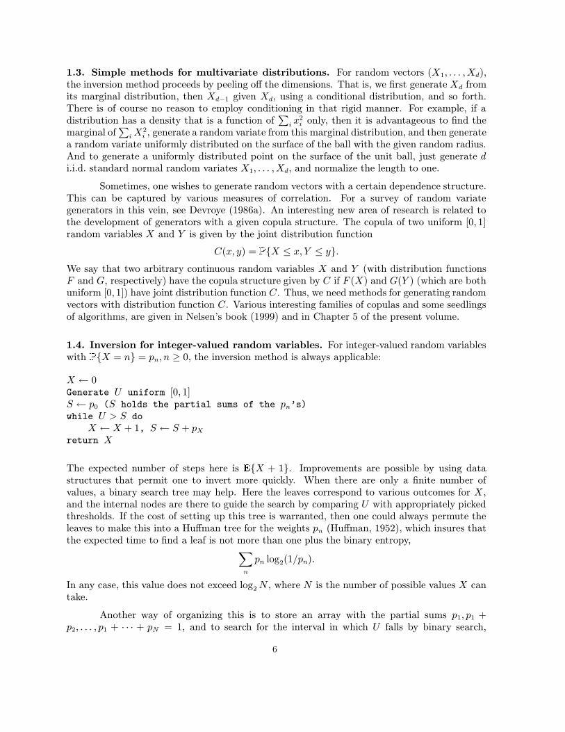
1.3. Simple methods for multivariate distributions. For random vectors (X1, . . . ,Xd),the inversion method proceeds by peeling off the dimensions. That is, we first generate Xd fromits marginal distribution, then Xd−1 given Xd, using a conditional distribution, and so forth.There is of course no reason to employ conditioning in that rigid manner. For example, if adistribution has a density that is a function of

∑i x

2i only, then it is advantageous to find the

marginal of∑

iX2i , generate a random variate from this marginal distribution, and then generate

a random variate uniformly distributed on the surface of the ball with the given random radius.And to generate a uniformly distributed point on the surface of the unit ball, just generate di.i.d. standard normal random variates X1, . . . ,Xd, and normalize the length to one.

Sometimes, one wishes to generate random vectors with a certain dependence structure.This can be captured by various measures of correlation. For a survey of random variategenerators in this vein, see Devroye (1986a). An interesting new area of research is related tothe development of generators with a given copula structure. The copula of two uniform [0, 1]random variables X and Y is given by the joint distribution function

C(x, y) =� {X ≤ x, Y ≤ y}.

We say that two arbitrary continuous random variables X and Y (with distribution functionsF and G, respectively) have the copula structure given by C if F (X) and G(Y ) (which are bothuniform [0, 1]) have joint distribution function C. Thus, we need methods for generating randomvectors with distribution function C. Various interesting families of copulas and some seedlingsof algorithms, are given in Nelsen’s book (1999) and in Chapter 5 of the present volume.

1.4. Inversion for integer-valued random variables. For integer-valued random variableswith

� {X = n} = pn, n ≥ 0, the inversion method is always applicable:

X ← 0Generate U uniform [0, 1]S ← p0 (S holds the partial sums of the pn’s)while U > S do

X ← X + 1, S ← S + pXreturn X

The expected number of steps here is� {X + 1}. Improvements are possible by using data

structures that permit one to invert more quickly. When there are only a finite number ofvalues, a binary search tree may help. Here the leaves correspond to various outcomes for X,and the internal nodes are there to guide the search by comparing U with appropriately pickedthresholds. If the cost of setting up this tree is warranted, then one could always permute theleaves to make this into a Huffman tree for the weights pn (Huffman, 1952), which insures thatthe expected time to find a leaf is not more than one plus the binary entropy,

∑

n

pn log2(1/pn).

In any case, this value does not exceed log2N , where N is the number of possible values X cantake.

Another way of organizing this is to store an array with the partial sums p1, p1 +p2, . . . , p1 + · · · + pN = 1, and to search for the interval in which U falls by binary search,

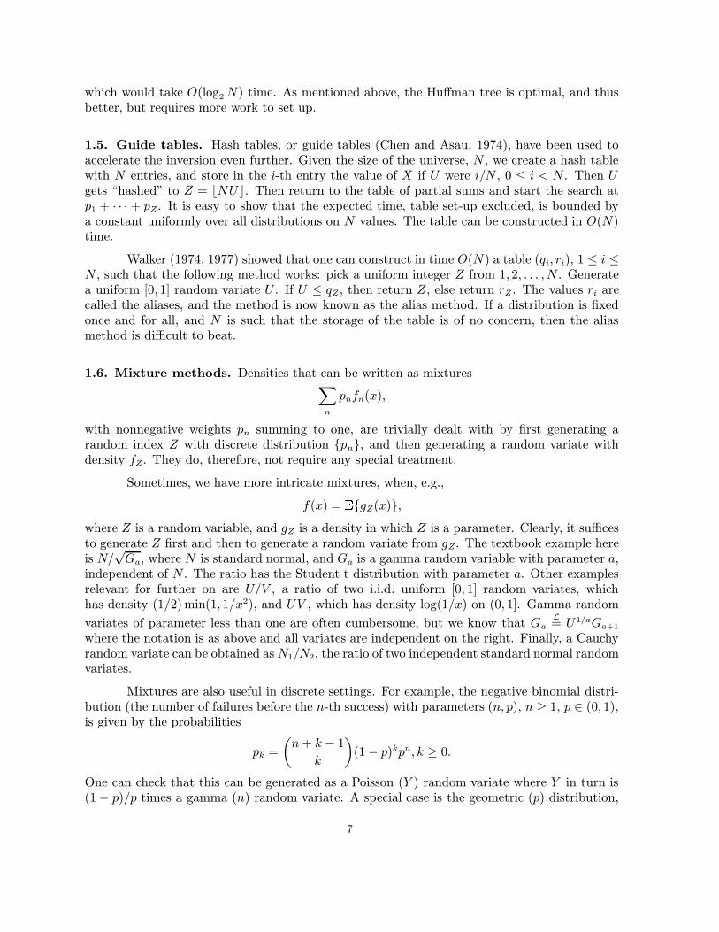
which would take O(log2 N) time. As mentioned above, the Huffman tree is optimal, and thusbetter, but requires more work to set up.

1.5. Guide tables. Hash tables, or guide tables (Chen and Asau, 1974), have been used toaccelerate the inversion even further. Given the size of the universe, N , we create a hash tablewith N entries, and store in the i-th entry the value of X if U were i/N , 0 ≤ i < N . Then Ugets “hashed” to Z = bNUc. Then return to the table of partial sums and start the search atp1 + · · · + pZ . It is easy to show that the expected time, table set-up excluded, is bounded bya constant uniformly over all distributions on N values. The table can be constructed in O(N)time.

Walker (1974, 1977) showed that one can construct in time O(N) a table (qi, ri), 1 ≤ i ≤N , such that the following method works: pick a uniform integer Z from 1, 2, . . . , N . Generatea uniform [0, 1] random variate U . If U ≤ qZ , then return Z, else return rZ . The values ri arecalled the aliases, and the method is now known as the alias method. If a distribution is fixedonce and for all, and N is such that the storage of the table is of no concern, then the aliasmethod is difficult to beat.

1.6. Mixture methods. Densities that can be written as mixtures∑

n

pnfn(x),

with nonnegative weights pn summing to one, are trivially dealt with by first generating arandom index Z with discrete distribution {pn}, and then generating a random variate withdensity fZ . They do, therefore, not require any special treatment.

Sometimes, we have more intricate mixtures, when, e.g.,

f(x) =� {gZ(x)},

where Z is a random variable, and gZ is a density in which Z is a parameter. Clearly, it sufficesto generate Z first and then to generate a random variate from gZ . The textbook example hereis N/

√Ga, where N is standard normal, and Ga is a gamma random variable with parameter a,

independent of N . The ratio has the Student t distribution with parameter a. Other examplesrelevant for further on are U/V , a ratio of two i.i.d. uniform [0, 1] random variates, whichhas density (1/2) min(1, 1/x2), and UV , which has density log(1/x) on (0, 1]. Gamma random

variates of parameter less than one are often cumbersome, but we know that GaL= U 1/aGa+1

where the notation is as above and all variates are independent on the right. Finally, a Cauchyrandom variate can be obtained as N1/N2, the ratio of two independent standard normal randomvariates.

Mixtures are also useful in discrete settings. For example, the negative binomial distri-bution (the number of failures before the n-th success) with parameters (n, p), n ≥ 1, p ∈ (0, 1),is given by the probabilities

pk =

(n+ k − 1

k

)(1− p)kpn, k ≥ 0.

One can check that this can be generated as a Poisson (Y ) random variate where Y in turn is(1− p)/p times a gamma (n) random variate. A special case is the geometric (p) distribution,

which is negative binomial (1, p). Here, though, it is better to use the inversion method whichcan be made explicit by the truncation operator: it suffices to take

blog1−p Uc,where U is uniform [0, 1].

1.7. The rejection method. Von Neumann (1951) proposed the rejection method, whichuses the notion of a dominating measure. Let X have density f on

�d. Let g be another density

with the property that for some finite constant c ≥ 1, called the rejection constant,

f(x) ≤ cg(x), x ∈ � d.

For any nonnegative integrable function h on� d, define the body of h as Bh = {(x, y) : x ∈

�d, 0 ≤ y ≤ h(x)}. Note that if (X,Y ) is uniformly distributed on Bh, then X has density

proportional to h. Vice versa, if X has density proportional to h, then (X,Uh(X)), where U isuniform [0, 1] and independent of X, is uniformly distributed on Bh. These facts can be usedto show the validity of the rejection method:

repeat

Generate U uniformly on [0, 1]Generate X with density g

until Ucg(X) ≤ f(X)return X

The expected number of iterations before halting is c, so the rejection constant must be keptsmall. This method requires some analytic work, notably to determine c, but one attractive fea-ture is that we only need the ratio f(x)/(cg(x)), and thus, cumbersome normalization constantsoften cancel out.

1.8. Rejection: a simple example. The rejection principle also applies in the discretesetting, so a few examples follow to illustrate its use in all settings. We begin with the standardnormal density. The start is an inequality such as

e−x2/2 ≤ eα2/2−α|x|.

The area under the dominating curve is eα2/2 × 2/α, which is minimized for α = 1. Generating

a random variate with the Laplace density e−|x| can be done either as SE, where S is a randomsign, and E is exponential, or as E1 −E2, a difference of two independent exponential randomvariables. The rejection algorithm thus reads:

repeat

Generate U uniformly on [0, 1]Generate X with with the Laplace density

until Ue1/2−|X| ≤ e−X2/2

return X

However, taking logarithms in the last condition, and noting that log(1/U) is expo-nential, we can tighten the code using a random sign S, and two independent exponentials,E1, E2:

Generate a random sign Srepeat

Generate E1, E2

until 2E2 > (E1 − 1)2

return X ← SE1

It is easy to verify that the rejection constant (the expected number of iterations) is√

2e/π ≈1.35.

1.9. Rejection: a more advanced example. Assume that f is a monotonically decreasingdensity on [0, 1], and define M = f(0). We could apply rejection with M as a bound:

repeat

Generate U uniformly on [0, 1]Generate X uniformly on [0, 1]

until UM ≤ f(X)return X

The expected number of iterations is M . However, the algorithm does not make any use of themonotonicity. As we know that f(x) ≤ min(M, 1/x), and the integral of the upper bound (orthe rejection constant) is 1 + logM , we can exponentially speed up the performance by basingour rejection on the latter bound. It is a simple exercise to show that the indefinite integral ofthe upper bound is {

Mx (0 ≤ x ≤ 1/M)1 + log(Mx) (1/M ≤ x ≤ 1).

A random variate can easily be generated by inversion of a uniform [0, 1] random variate U : ifU ≤ 1/(1 + logM), return (1 + logM)U/M , else return (1/M) exp((1 + logM)U − 1). Thus,we have the improved algorithm:

repeat

Generate U, V independently and uniformly on [0, 1].Set W = V (1 + logM).If W ≤ 1 then set X ←W/M

else set X ← exp(WU − 1)/Muntil U min(M, 1/X) ≤ f(X)return X

It is possible to beat even this either by spending more time setting up (a one-time cost) orby using additional information on the density. In the former case, partition [0, 1] into k equalintervals, and invest once in the calculation of f(i/k), 0 ≤ i < k. Then the histogram functionof height f(i/k) on [i/k, (i + 1)/k) dominates f and can be used for rejection purposes. This

requires the bin probabilities pi = f(i/k)/∑k−1

j=0 f(j/k). Rejection can proceed as follows:

repeat

Generate U, V independently and uniformly on [0, 1]Generate Z on {0, 1, . . . , k − 1} according to the probabilities {pi}.Set X = (Z + V )/k.

until Uf(Z/k) ≤ f(X)return X

Here the area under the dominating curve is at most one plus the area sandwiched between f andit. By shifting that area over to the left, bin by bin, one can bound it further by 1+M/k. Thus,we can adjust k to reduce the rejection constant at will. For example, a good choice wouldbe k = dMe. The expected time per variate would be O(1) if we can generate the randominteger Z in time O(1). This can be done, but only at the expense of the set-up of a tableof size k (see above). In one shot situations, this is a prohibitive expense. In Devroye (1986),methods based on partitioning the density in slabs are called strip methods. Early papers in thisdirection include Ahrens and Dieter (1989), Ahrens (1993, 1995), Marsaglia and Tsang (1984)and Marsaglia, Maclaren and Bray (1964).

Assume next that we also know the mean µ of f . Then, even dropping the requirementthat f be supported on [0, 1], we have

µ =

∫ ∞

0

yf(y)dy ≥ f(x)

∫ x

0

ydy = f(x)x2/2.

Hence,

f(x) ≤ min

(M,

2µ

x2

).

The integral of the upper bound from 0 to x is{Mx 0 ≤ x <

√2µ/M

2√

2µM − 2µx

x ≥√

2µ/M .

The area under the upper bound is therefore 2√

2µM . To generate a random variate withdensity proportional to the upper bound, we can proceed in various ways, but it is easy to checkthat

√2µ/MU1/U2 fits the bill, where U1, U2 are independent uniform [0, 1] random variables.

Thus, we summarize:

repeat

Generate U, V,W independently and uniformly on [0, 1].

Set X =√

2µ/MV/W.

until UM min (1, (W/V )2) ≤ f(X)return X

This example illustrates the development of universal generators, valid for large classesof densities, as a function of just a few parameters. The reader will be able to generalize theabove example to unimodal densities with known r-th moment about the mode. The examplegiven above applies with trivial modifications to all unimodal densities, and the expected timeis bounded by a constant times

√f(m)

� {|X −m|}, where m is the mode. For example, thegamma density with parameter a ≥ 1 has mean a, and mode at a − 1, with f(a− 1) ≤ C/

√a

for some constant C, and� {|X− (a−1)|} ≤ C ′

√a for another constant C ′. Thus, the expected

time taken by our universal algorithm takes expected time bounded by a constant, uniformlyover a ≥ 1. We say that the algorithm is uniformly fast over this class of densities.

1.10. The alternating series method. To apply the rejection method, we do not really needto know the ratio f(x)/(cg(x)) exactly. It suffices that we have an approximation φn(x) thattends, as n → ∞, to f(x)/(cg(x)), and for which we know a monotone error bound εn(x) ↓ 0.In that case, we let n increase until for the first time, either

U ≤ φn(X)− εn(X)

(in which case we accept X), or

U ≥ φn(X) + εn(X)

(in which case we reject X). Equivalently, we have computable bounds ξn(x) and ψn(x) withthe property that ξn(x) ↑ f(x)/(cg(x)) and ψn(x) ↓ f(x)/(cg(x)) as n → ∞. This approachis useful when the precise computation of f is impossible, e.g., when f is known as infiniteseries or when f can never be computed exactly using only finitely many resources. It was firstdeveloped for the Kolmogorov-Smirnov limit distribution in Devroye (1981a). For another useof this idea, see Keane and O’Brien’s Bernoulli factory (1994).

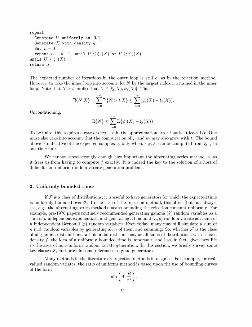
repeat

Generate U uniformly on [0, 1]Generate X with density gSet n = 0repeat n← n+ 1 until U ≤ ξn(X) or U ≥ ψn(X)

until U ≤ ξn(X)return X

The expected number of iterations in the outer loop is still c, as in the rejection method.However, to take the inner loop into account, let N be the largest index n attained in the innerloop. Note that N > t implies that U ∈ [ξt(X), ψt(X)]. Thus,

� {N |X} =∞∑

t=0

� {N > t|X} ≤∞∑

t=0

(ψt(X)− ξt(X)).

Unconditioning,

� {N} ≤∞∑

t=0

� {ψt(X)− ξt(X)}.

To be finite, this requires a rate of decrease in the approximation error that is at least 1/t. Onemust also take into account that the computation of ξt and ψt may also grow with t. The boundabove is indicative of the expected complexity only when, say, ξt can be computed from ξt−1 inone time unit.

We cannot stress strongly enough how important the alternating series method is, asit frees us from having to compute f exactly. It is indeed the key to the solution of a host ofdifficult non-uniform random variate generation problems.

2. Uniformly bounded times

If F is a class of distributions, it is useful to have generators for which the expected timeis uniformly bounded over F . In the case of the rejection method, this often (but not always,see, e.g., the alternating series method) means bounding the rejection constant uniformly. Forexample, pre-1970 papers routinely recommended generating gamma (k) random variables as asum of k independent exponentials, and generating a binomial (n, p) random variate as a sum ofn indepoendent Bernoulli (p) random variables. Even today, many may still simulate a sum ofn i.i.d. random variables by generating all n of them and summing. So, whether F is the classof all gamma distributions, all binomial distributions, or all sums of distributions with a fixeddensity f , the idea of a uniformly bounded time is important, and has, in fact, given new lifeto the area of non-uniform random variate generation. In this section, we briefly survey somekey classes F , and provide some references to good generators.

Many methods in the literature are rejection methods in disguise. For example, for real-valued random variates, the ratio of uniforms method is based upon the use of bounding curvesof the form

min

(A,

B

x2

).

The area under the bounding curve is 4√AB, and a random variate with density proportional

to it can be generated as√B/ASU/V , where S is a random sign, and U, V are independent

uniform [0, 1] random variates. The method is best applied after shifting the mode or mean ofthe density f to the origin. One could for example use

A = supx

f(x), B = supx

x2f(x).

In many cases, such as for mode-centered normals, gamma, beta, and Student t distributions,the rejection constant 4

√AB is uniformly bounded over all or a large part of the parameter

space. Discretized versions of it can be used for the Poisson, binomial and hypergeometricdistributions.

Uniformly fast generators have been obtained for all major parametric families. Inter-esting contributions include the gamma generators of Cheng (1977), Le Minh (1988), Marsaglia(1977), Ahrens and Dieter (1982), Cheng and Feast (1979, 1980), Schmeiser and Lal (1980),Ahrens, Kohrt and Dieter (1983), and Best (1983), the beta generators of Ahrens and Dieter(1974), Zechner and Stadlober (1993), Best (1978), and Schmeiser and Babu (1980), the bino-mial methods of Stadlober (1988, 1989), Ahrens and Dieter (1980), Hormann (1993), and Ka-chitvichyanukul and Schmeiser (1988, 1989), the hypergeometric generators of Stadlober (1988,1990), and the code for Poisson variates by Ahrens and Dieter (1980), and Hormann (1993).Some of these algorithms are described in Devroye (1986a), where some additional uniformlyfast methods can be found.

All the distributions mentioned above are log-concave, and it is thus no surprise that wecan find uniformly fast generators. The emphasis in most papers is on the details, to squeezethe last millisecond out of each piece of code. To conclude this section, we will just describe arecent gamma generator, due to Marsaglia and Tsang (2001). It uses almost-exact inversion.Its derivation is unlike anything in the present survey, and shows the careful planning that goesinto the design of a nearly perfect generator. The idea is to consider a monotone transformationh(x), and to note that if X has density

eg(x) def=h(x)a−1e−h(x)h′(x)

Γ(a),

then Y = h(X) has the gamma (a) density. If g(x) is close to c−x2/2 for some constant c, thena rejection method from a normal density can be developed. The choice suggested by Marsagliaand Tsang is

h(x) = d(1 + cx)3 , −1/c < x <∞,with d = a− 1/3, c = 1/

√9d. In that case, simple computations show that

g(x) = 3d log(1 + cx)− d(1 + cx)3 + d+ C , −1/c < x <∞,for some constant C. Define w(x) = −x2/2− g(x). Note that w′(x) = −x− 3dc

1+cx+ 3dc(1 + cx)2,

w′′(x) = −1 + 3dc2

(1+cx)2 + 6dc2(1 + cx), w′′′(x) = − 6dc3

(1+cx)3 + 6dc3. The third derivative is zero at

(1 + cx)3 = 1, or x = 0. Thus, w′′ reaches a minimum there, which is −1 + 9dc2 = 0. Therefore,by Taylor’s series expansion, and the fact that w(0) = −C, w′(0) = 0, we have w(x) ≥ C.Hence,

eg(x) ≤ eC−x2/2

and the rejection method immediately yields the following:

d← a− 1/3

c← 1/√

9drepeat

generate E exponential

generate X normal

Y ← d(1 + cX)3

until −X2/2− E ≤ d log(Y )− Y + dreturn Y

We picked d so that∫eg−C is nearly maximal. By the transformation y = d(1 + cx)3 and by

Stirling’s approximation, as d→∞,∫ ∞

−1/c

eg(x)−Cdx =

∫ ∞

0

yd−2/3ed−y

3cdd+1/3dy =

Γ(d+ 1/3)ed

3cdd+1/3

∼ (1 + 1/3d)d+1/3√

2π

3ce1/3√d+ 1/3

∼√

18πd

3√d+ 1/3

∼√

2π.

Using∫e−x

2/2 dx =√

2π, we note that the asymptotic (as a → ∞) rejection constant is 1: wehave a perfect fit! Marsaglia and Tsang recommend the method only for a ≥ 1. For additionalspeed, a squeeze step (or quick acceptance step) may be added.

3. Universal generators

It is quite important to develop generators that work well for entire families of distri-butions. An example of such development is the generator for log concave densities given inDevroye (1984a), that is, densities for which log f is concave. On the real line, this has severalconsequences: these distributions are unimodal and have sub-exponential tails. Among the logconcave densities, we find the normal densities, the gamma family with parameter a ≥ 1, theWeibull family with parameter a ≥ 1, the beta family with both parameters ≥ 1, the expo-nential power distribution with parameter ≥ 1 (the density being proportional to exp(−|x|a)),the Gumbel or double exponential distribution (kk exp(−kx − ke−x)/(k − 1)! is the density,k ≥ 1 is the parameter), the generalized inverse Gaussian distribution, the logistic distribution,Perks’ distribution (with density proportional to 1/(ex + e−x + a), a > −2), the hyperbolic se-cant distribution (with distribution function (2/π) arctan(ex)), and Kummer’s distribution (fora definition, see Devroye, 1984a). Also, we should consider simple nonlinear transformationsof other random variables. Examples include arctanX with X Pearson IV, log |X| (X beingStudent t for all parameters), logX (for X gamma, all parameters), logX (for X log-normal),logX (for X Pareto), log(X/(1−X)) (for all beta variates X), and logX (for X beta (a, b) forall a > 0, b ≥ 1).

In its most primitive version, assuming one knows that a mode occurs at m, we considerthe generation problem for the normalized random variable Y = f(m)(X−m). One may obtainX as m + Y/f(m). The new random variable has a mode at 0 of value 1. Call its density g.Devroye (1984a) showed that

g(y) ≤ min(1, e1−|y|) .

The integral of the upper bound is precisely 4. Thus, the rejection constant will be 4, uniformlyover this vast class of densities. A random variable with density proportional to the upperbound is generated by first flipping a perfect coin. If it is heads, then generate (1 +E)S, whereE is exponential, and S is another perfect coin. Otherwise generate US, where U is uniform[0, 1] and independent of S. The algorithm is as follows:

repeat

Generate U (a uniform on [0, 1]), E (exponential), and S (a fair random bit).

Generate a random sign S ′.If S = 0 then Y ← 1 + E

else Y ← V , V uniform [0, 1]Set Y ← Y S′

until U min(1, e1−|Y |) ≤ g(Y )

return Y

Various improvements can be found in the original paper. In adaptive rejection sampling,Gilks and Wild (1992) bound the density adaptively from above and below by a number ofexponential pieces, to reduce the integral under the bounding curve. If we denote the logconcave density by f , and if f ′ is available, then for all x, log-concavity implies that

log f(y) ≤ log f(x) + (y − x)f ′(x)

f(x), y ∈ �

.

This is equivalent to

f(y) ≤ f(x)e(y−x)f ′(x)/f(x), y ∈ �.

Assume that we have already computed f at k points. Then we can construct k+ 1 exponentialpieces (with breakpoints at those k points) that bound the density from above, and in fact,sampling from the piecewise exponential dominating curve is easily carried out by inversion.The integral under a piece anchored at x and spanning [x, x + δ) is

f 2(x)(eδf

′(x)/f(x) − 1)

f ′(x).

Gilks and Wild also bound f from below. Assume that y ∈ [x, x′], where x and x′ are two ofthose anchor points. Then

log(f(y)) ≥ log(f(x)) +y − xx′ − x (log(f(x′))− log(f(x))) .

The lower bound can be used to avoid the evaluation of f most of the time when accepting orrejecting. It is only when f is actually computed that a new point is added to the collection toincrease the number of exponential pieces.

Hormann (1995) shows that it is best to add two exponential tails that touch g atthe places where g(x) = 1/e, assuming that the derivative of g is available. In that case,the area under the bounding curve is reduced to e/(e − 1) ≈ 1.582. Hormann and Derflinger(1994) and Hormann (1995) (see also Leydold (2000a, 2000b, 2001) and Hormann, Leydoldand Derflinger (2004)) define the notion of Tc-concavity, related to the concavity of −1/(f(x))c,where 0 < c < 1. For example, the Student t distribution of parameter ≥ 1 is T1/2-concave.Similar universal methods related to the one above are developed by them. Rejection is done

from a curve with polynomial tails, and the rejection constant is(1− (1− c)1/c−1

)−1. The

notion of T -convexity proposed by Evans and Swartz (1996, 2000) is useful for unboundeddensities.

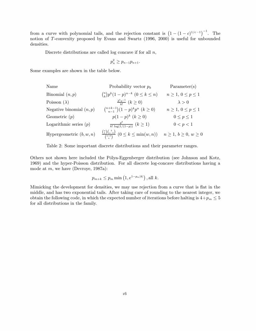
Discrete distributions are called log concave if for all n,

p2n ≥ pn−1pn+1.

Some examples are shown in the table below.

Name Probability vector pk Parameter(s)

Binomial (n, p)(nk

)pk(1− p)n−k (0 ≤ k ≤ n) n ≥ 1, 0 ≤ p ≤ 1

Poisson (λ) λke−λ

k!(k ≥ 0) λ > 0

Negative binomial (n, p)(n+k−1n−1

)(1− p)kpn (k ≥ 0) n ≥ 1, 0 ≤ p ≤ 1

Geometric (p) p(1− p)k (k ≥ 0) 0 ≤ p ≤ 1

Logarithmic series (p) pk

k! log(1/(1−p)) (k ≥ 1) 0 < p < 1

Hypergeometric (b, w, n)(wk)(

bn−k)

(w+bn )

(0 ≤ k ≤ min(w, n)) n ≥ 1, b ≥ 0, w ≥ 0

Table 2: Some important discrete distributions and their parameter ranges.

Others not shown here included the Polya-Eggenberger distribution (see Johnson and Kotz,1969) and the hyper-Poisson distribution. For all discrete log-concave distributions having amode at m, we have (Devroye, 1987a):

pm+k ≤ pm min(1, e1−pm|k|) , all k.

Mimicking the development for densities, we may use rejection from a curve that is flat in themiddle, and has two exponential tails. After taking care of rounding to the nearest integer, weobtain the following code, in which the expected number of iterations before halting is 4+pm ≤ 5for all distributions in the family.

Compute w ← 1 + pm/2 (once)

repeat

Generate U, V,W uniformly on [0, 1], and let S be a random sign.

If U ≤ w1+w

then Y ← V w/pmelse Y ← (w − log V )/pm

X ← S round(Y )until W min (1, ew−pmY ) ≤ pm+X/pmreturn m+X

We can tighten the rejection constant further to 2 + pm for log concave distributions that aremonotonically decreasing. The disadvantage in the code is the requirement that pm must becomputed.

The development for log-concave distributions can be aped for other classes. For ex-ample, the adaptive rejection method of Gilks and Wild can be used for unimodal densitieswith known mode m. One just needs to replace the exponential upper and lower bounds byhistograms. This is covered in an exercise in Devroye (1986a). General algorithms are knownfor all Lipschitz densities with known bounds on the Lipschitz constant C and variance σ2, andall unimodal densities with mode at m, and variance bounded by σ2, to give two examples (seeDevroye, 1984b, 1986a).

4. Indirect problems

A certain amount of work is devoted to indirect problems, in which distributions are notdescribed by their density, distribution function or discrete probability vector. A partial listfollows, with brief descriptions on how the solutions may be constructed.

4.1. Characteristic functions. If the characteristic function

ϕ(t) =� {

eitX}

is known in black box format, very little can be done in a universal manner. In particularcases, we may have enough information to be able to deduce that a density exists and that it isbounded in a certain way. For example, from the inversion formula

f(x) =1

2π

∫ϕ(t)e−itxdt,

we deduce the bounds

supx

f(x) ≤Mdef=

1

2π

∫|ϕ(t)|dt

and

supx

x2f(x) ≤M ′ def=

1

2π

∫|ϕ′′(t)|dt

Thus, we havef(x) ≤ min(M,M ′/x2),

a bound that is easily dealt with by rejection. In principle, then, rejection can be used, with f(x)approximated at will by integral approximations based on the inversion integral. This method

requires bounds on the integral approximation, and these depend in turn on the smoothness ofϕ. Explicit bounds on some smoothness parameters must be available. There are descriptionsand worked out examples in Devroye (1981b, 1986b, 1988). Devroye (1988) uses this methodto simulate the sum Sn of n i.i.d. random variables with common characteristic function ϕ inexpected time not depending upon n, as Sn has characteristic function ϕn.

Polya showed that any convex function ϕ on the positive halfline that decreases from 1to 0 is the characteristic function of a symmetric random variable if we extend it to the realline by setting ϕ(−t) = ϕ(t). These distributions correspond to random variables distributedas Y/Z, where Y and Z are independent, Y has the de la Vallee-Poussin density

1

2π

(sin(x/2)

x/2

)2

, x ∈ �

(for which random variate generation by rejection is trivial), and Z has distribution function onthe positive halfline given by 1− ϕ(t) + tϕ′(t). See Dugue and Girault (1955) for this propertyand Devroye (1984a) for its implications in random variate generation. Note that we havemade a space warp from the complex to the real domain. This has unexpected corollaries. Forexample, if E1, E2 are independent exponential random variables, U is a uniform [0, 1] randomvariable, and α ∈ (0, 1], then Y/Z with

Z = (E1 +E2

�U<α)

1α

is symmetric stable of parameter (α), with characteristic function e−|t|α

. The Linnik-Lahadistribution (Laha, 1961) with parameter α ∈ (0, 1] is described by

ϕ(t) =1

1 + |t|α .

Here Y/Z with

Z =

(α+ 1−

√(α+ 1)2 − 4αU

2U− 1

) 1α

has the desired distribution.

4.2. Fourier coefficients. Assume that the density f , suitably scaled and translated, issupported on [−π, π]. Then the Fourier coefficients are given by

ak =�{

cos(kX)

π

}, bk =

�{

sin(kX)

π

}, k ≥ 0.

They uniquely describe the distribution. If the series absolutely converges,∑

k

|ak|+ |bk| <∞,

then the following trigonometric series is absolutely and uniformly convergent to f :

f(x) =a0

2+∞∑

k=1

(ak cos(kx) + bk sin(kx)).

If we only use terms with index up to n, then the error made is not more than

Rn+1 =∞∑

k=n+1

√a2k + b2

k.

If we know bounds on Rn, then one can use rejection with an alternating series method togenerate random variates (Devroye, 1989).

A particularly simple situation occurs when only the cosine coefficients are nonzero, asoccurs for symmetric distributions. Assume furthermore that the Fourier cosine series coeffi-cients ak are convex and ak ↓ 0 as k → ∞. Even without absolute convergence, the Fouriercosine series converges, and can in fact be rewritten as follows:

f(x) =

∞∑

k=0

π(k + 1)∆2akKk(x),

where ∆2ak = ak+2 − 2ak+1 + ak (a positive number, by convexity), and

Kk(x) =1

2π(k + 1)

(sin((k + 1)x/2)

sin(x/2)

)2

, |x| ≤ π,

is the Fejer kernel. As Kk(x) ≤ min((k + 1)/4, π/(2(k+ 1)x2), random variates from it can begenerated in expected time uniformly bounded in k by rejection. Thus, the following simplealgorithm does the job:

Generate U uniformly on [0, 1].Z ← 0, S ← π∆2a0.

while U > S do

Z ← Z + 1.S ← S + π(Z + 1)∆2aZ.

Generate X with Fejer density KZ.

return X

4.3. The moments are known. Let µn denote the n-th moment of a random variable X.One could ask to generate a random variate when for each n, µn is computable (in a black box).Again, this is a nearly impossible problem to solve, unless additional information is available.For one thing, there may not be a unique solution. A sufficient condition that guarantees theuniqueness is Carleman’s condition

∞∑

n=0

|µ2n|−1

2n =∞

(see Akhiezer, 1965). Sufficient conditions in terms of a density f exist, such as Krein’s condition∫ − log(f(x))

1 + x2dx =∞,

combined with Lin’s condition, applicable to symmetric and differentiable densities, which statesthat x|f ′(x)|/f(x) ↑ ∞ as x → ∞ (Lin, 1997, Krein, 1944, Stoyanov, 2000). Whenever thedistribution is of compact support, the moments determine the distribution. In fact, there are

various ways for reconstructing the density from the moments. An example is provided by theseries

f(x) =∞∑

k=0

akφj(x), |x| ≤ 1,

where φk is the Legendre polynomial of degree k, and ak is a linear function of all moments upto the k-th. The series truncated at index n has an error not exceeding

Cr∫ |f (r+1)|

(1− x2)1/4nr−1/2

where r is an integer and Cr is a constant depending upon r only (Jackson, 1930). Rejectionwith dominating curve of the form C ′/(1− x2)1/4 (a symmetric beta) and with the alternatingseries method can thus lead to a generator (Devroye, 1989).

The situation is much more interesting when X is supported on the positive integers.Let

Mr =� {X(X − 1) · · · (X − r + 1)}

denote the r-th factorial moment. Then, approximate pj =� {X = j} by

pnj =1

j!

n∑

i=0

(−1)iMj+i

i!.

Note that pnj ≥ pj for n even, pnj ≤ pj for n odd, and pnj → pj as n → ∞ provided that� {(1 + u)X} <∞ for some u > 0. Under this condition, an alternating series rejection methodcan be implemented, with a dominating curve suggested by the crude bound

pj ≤ min

(1,µrjr

).

In fact, we may even attempt inversion, as the partial sums p0 + p1 + · · ·+ pj are available withany desired accuracy: it suffices to increase n until we are absolutely sure in which interval agiven uniform random variate U lies. For more details, see Devroye (1991).

4.4. The moment generating function. For random variables on the positive integers, asin the previous section, we may have knowledge of the moment generating function

k(s) = p0 + p1s+ p2s2 + · · · = � {

sX}.

Here we have trivially,

pj ≤k(s)

sj,

where s > 0 can be picked at will. Approximations for pj can be constructed based on differencesof higher orders. For example, if we take t > 0 arbitrary, then we can define

pnj =

∑j

i=0(−1)j−i(ji

)k(it)

j!tj

and note that

0 ≤ pnj − pj ≤1

(1− jt)j+1− 1.

This is sufficient to apply the alternating series method (Devroye, 1991).

4.5. An infinite series. Some densities are known as infinite series. Examples include thetheta distribution (Renyi and Szekeres, 1967) with distribution function

F (x) =∞∑

j=−∞(1− 2j2x2)e−j

2x2

=4π5/2

x3

∞∑

j=1

j2e−π2j2/x2

, x > 0,

and the Kolmogorov-Smirnov distribution (Feller, 1948) with distribution function

F (x) = 1− 2∞∑

j=1

(−1)je−2j2x2

, x > 0.

In the examples above, it is relatively straightforward to find tight bounding curves, and toapply the alternating series method (Devroye, 1981a and 1997).

4.6. Hazard rates. Let X be a positive random variable with density f and distributionfunction F . Then the hazard rate, the probability of instantaneous death given that one is stillalive, is given by

h(x) =f(x)

1− F (x).

Assume that one is given h (note that h ≥ 0 must integrate to∞). Then f can be recovered asfollows:

f(x) = h(x)e−∫ x

0 h(y)dy.

This may pose a problem for random variate generation. Various algorithms for simulation inthe presence of hazard rates are surveyed by Devroye (1986c), the most useful among which isthe thinning method of Lewis and Shedler (1979): assume that h ≤ g, where g is another hazardrate. If 0 < Y1 < Y2 < · · · is a nonhomogeneous Poisson point process with rate function g, andU1, U2, . . . is a sequence of independent uniform [0, 1] random variables, independent of the Yi’s,and if i is the smallest index for which Uig(Yi) ≤ f(Yi), then X = Yi has hazard rate h.

This is not a circular argument if we know how to generate a nonhomogeneous Poissonpoint process with rate function g. Define the cumulative rate function G(x) =

∫ x0g(y)dy. Let

E1, E2, . . . be i.i.d. exponential random variables with partial sums Si =∑i

j=1 Ej . Then the

sequence Yi = Ginv(Si), i ≥ 1, is a nonhomogeneous Poisson point process with rate g. Thus,the thinning method is a Poisson process version of the rejection method.

If h(0) is finite, and X has the given hazard rate, then for a dhr (decreasing hazard rate)distribution, we can use g = h(0). In that case, the expected number of iterations before haltingis

� {h(0)X}. However, we can dynamically thin (Devroye, 1986c) by lowering g as values h(Yi)trickle in. In that case, the expected time is finite when X has a finite logarithmic moment,and in any case, it is not more than 4 +

√24

� {h(0)X}.

4.7. A distributional identity. The theory of fixed points and contractions can be used toderive many limit laws in probability (see, e.g., Rosler and Ruschendorf, 2001). These often aredescribed as distributional identities known to have a unique solution. For example, the identity

XL= W (X + 1)

where W is a fixed random variable on [0, 1] and X ≥ 0 sometimes has a unique solution for X.By iterating the identity, we see that if the solution exists, it can be represented as

XL= W1 +W1W2 +W1W2W3 + · · · ,

where the Wi’s are i.i.d. These are known as perpetuities (Vervaat, 1979, Goldie and Grubel,1996). Some more work in the complex domain can help out: for example, when W = U 1/α,where U is uniform [0, 1] and α > 0 leads to the characteristic function

ϕ(t) = eα∫ 1

0eitx−1x dx.

For the particular case α = 1, we have Dickman’s distribution (Dickman, 1930), which is thelimit law of

1

n

n∑

i=1

iZi

where Zi is Bernoulli (1/i). None of the three representations above (infinite series, Fouriertransform, limit of a discrete sum) gives a satisfactory path to an exact algorithm (althoughapproximations are trivial). The solution in Devroye (2001) uses the characteristic functionrepresentation in an alternating series method, after first determining explicit bounds on thedensity of f that can be used in the rejection method. A simpler approach to this particulardistributional identity is still lacking, and a good exact solution for distributional identities ingeneral is sorely needed.

Consider distributional identities of the form

XL= f1(U)X + f2(U)X ′ + f3(U)

where the fi’s are known functions, U is a uniform random variate, and X,X ′ are i.i.d. and inde-pendent of U . Exact generation here is approached by discretization in Devroye and Neininger(2002): suitably discretize the distributions of fi(U), and apply the map n times, starting witharbitrary values (say, zero) for X,X ′. If Xn is the random variable thus obtained, and Fn is itsdistribution function, note that Fn can be calculated as a sum, due to the discretization. Sometheoretical work is needed (which involves parameters of the fi’s) to obtain inequalities of thetype ∣∣∣∣

Fn(x+ δ)− Fn(x)

δ− f(x)

∣∣∣∣ ≤ Rn(x),

where Rn(x) is explicitly known and can be made as small as desired by appropriate choice ofall the parameters (the discretization, δ and n). This suffices to apply the alternating seriesmethod, yet again.

4.8. Kolmogorov and Levy measures. Infinitely divisible distributions (Sato, 2000) haveseveral representations. One of them is Kolmogorov’s canonical representation for the logarithmof the characteristic function:

logϕ(t) = ict+

∫eitx − 1− itx

x2dK(x),

where K(−∞) = 0, K ↑, and K(∞)−K(−∞) = σ2. Thus, K can be viewed as some sort ofmeasure. When K puts mass σ2 at the origin, then we obtain the normal distribution. WhenK puts mass λ at 1, then the Poisson (λ) distribution is obtained. However, in general, weonly have representations as integrals. For example, with c = 1, K(x) = min(x2/2, 1/2) on thepositive halfline, we obtain Dickman’s distribution,

logϕ(t) =

∫ 1

0

eitx − 1

xdx.

Bondesson (1982) presents approximations when one is given the measure K. Basically,if K is approximated by n point masses each of total weight σ2/n, then the characteristicfunction can be written as a product, where each term in the product, assuming c = 0, is of theform

eα(eitβ−1−itβ)

for fixed values of α and β. This is the characteristic function of β(X − α) where X is Poisson(α). Thus, approximations consist of sums of such random variables. However, if the truedistribution has a density, such discrete approximations are not acceptable.

5. Random processes

A random process Xt, t ∈�d, can not be produced using a finite amount of resources, as

the domain of the index is uncountable. So, it is customary to say that we can generate a randomprocess exactly if for any k, and for any set of indices t1, . . . , tk, we can generate the randomvector (Xt1 , . . . ,Xtk) exactly. Often, these points are nicely spaced out. In many processes,we have particularly elegant independence properties. For example, for all Levy processes andsetting d = 1, we have X0 = 0, Xt1 ,Xt2 − Xt1 , . . . ,Xtk − Xtk−1

independent, and furthermore,less important to us, the distribution of Xs+t−Xs depends upon t only and we have continuity:� {|Xs+t − Xs| > ε} → 0 as t ↓ 0 for all ε > 0. With that independence alone, we can thusgenerate each piece independently. When k is large, to protect against a proliferation of errors,it is wise to use a dyadic strategy: first generate the process at tk/2, then at tk/4 and t3k/4, andso on. The dyadic trick requires that we know the distribution of Xs+u − Xs conditional onXs+t −Xs for all 0 ≤ u ≤ t.

An example suffices to drive home this point. In Brownian motion (S(t), t ≥ 0) (a Levyprocess), we have differences Xs+t − Xs that are distributed as

√tN , where N is a standard

normal random variable. Furthermore, setting u = t/2, we see that

Xs+t −Xs = (Xs+t −Xs+u) + (Xs+u −Xs)

is a sum of two independent normal random variables with variances t/2 each. Conditional on

Xs+t −Xs, Xs+u −Xs thus is distributed as

Xs+t −Xs

2+

√t

2N.

Therefore, the dyadic trick applies beautifully. In the same manner, one can simulate theBrownian bridge on [0, 1], B(t) = S(t)− tS(1). For the first systematic examples of the use ofthis splitting trick, see Caflish, Morokoff and Owen (1997), and Fox (1999).

In a more advanced example, consider a gamma process S(t), where S(t) is distributedas a gamma random variable with parameter αt. This is not a Levy process, but rather a mono-tonically increasing process. We have the following recursive property: given S(t), S(t/2)/S(t)is distributed as a symmetric beta with parameter αt/2. This allows one to apply the dyadictrick.

Perhaps the most basic of all processes is the Poisson point process. These processesare completely described by an increasing sequence of occurrences 0 < X1 < X2, · · ·. In ahomogeneous point process of density λ, the inter-occurrence distances are i.i.d. and distributedas exponentials of mean 1/λ. In a nonhomegenoeous Poisson point process of density λ(t), a

nonnegative function, the integrals∫ Xi+1

Xiλ(t) dt are i.i.d. exponential. If Λ(t) =

∫ t0λ(t)dt, then it

is easy to see that Xi+1−Xi is distributed as Λinv(Λ(Xi)+E)−Xi, where E is exponential. Wealready discussed sampling by thinning (rejection) for this process elsewhere. This process viewalso yields a simple but not uniformly fast generator for the Poisson distribution: if E1, E2, . . .are i.i.d. exponential random variables, and X is the smallest integer such that

X+1∑

i=1

Ei > λ,

then X is Poisson (λ), as we are just counting the number of occurrences of a unit densityhomogeneous Poisson point process in the interval [0, λ]. By noting that an exponential isdistributed as the logarithm of one over a uniform, we see that we may equivalently generatei.i.d. uniform [0, 1] random variables U1, U2, . . . and let X be the smallest integer such that

X+1∏

i=1

Ui < e−λ.

This is the so-called product method for Poisson random variates.

6. Markov chain methodology

We say that we generate X by the Markov chain method if we can generate a Markovchain Xn, n ≥ 1 with the property that

limn→∞

� {Xn ≤ z} =� {X∞ ≤ z},

at all z at which the function� {X∞ ≤ z} is continuous (here ≤ is to be taken componentwise).

We write XnL→ X∞, and say that Xn converges in distribution to X∞. This is a weak notion,

as Xn may be discrete and X∞ continuous. For example, we may partition�d into a grid of

cells of sides 1/n1/(2d), and let pu be the probability content of cell u. Let Xn be the midpoint of

cell u, where cell u is selected with probability pu. A simple exercise shows that XnL→ X∞ for

any distribution of X∞. Yet, Xn is discrete, and X∞ may have any type of distribution. Oneneeds of course a way of computing the pu’s. For this, knowledge of the distribution function Fof X∞ at each point suffices, as pu can be written as a finite linear combination of the values ofF at the vertices of the cell u. If Xn needs to have a density, one can define Xn as a uniformvariate over the cell u, picked as above. In the latter case, if X∞ has any density, we have astronger kind of convergence, namely convergence in total variation (see below), by virtue ofthe Lebesgue density theorem (Wheeden and Zygmund, 1977; Devroye, 1987b). A good generalreference for this section is Haggstrom (2002).

The paradigm described in the previous paragraph is a special case of what one could callthe limit law method. Many processes, such as averages, maxima, and so forth, have asymptoticdistributions that are severely restricted (e.g., averages of independent random variables have astable limit law). Markov chains can easily be molded to nearly all distributions we can imagine,hence the emphasis on them as a tool.

In the exact Markov chain method, we can use properties of the Markov chain to generate

a random variateXT , whereXTL= X∞, where we recall that

L= denotes “is distributed as”. There

are a certain number of tricks that one can use to define a computable stopping time T . Thefirst one was the so-called coupling from the past method of Propp and Wilson (1996), whichhas been shown to work well for discrete Markov chains, especially for the generation of randomcombinatorial objects. For general continuous distributions, a sufficiently general constructionof stopping times is still lacking.

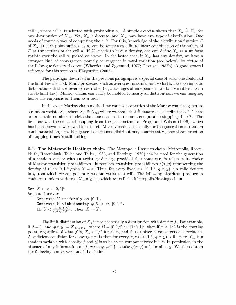
6.1. The Metropolis-Hastings chain. The Metropolis-Hastings chain (Metropolis, Rosen-bluth, Rosenbluth, Teller and Teller, 1953, and Hastings, 1970) can be used for the generationof a random variate with an arbitrary density, provided that some care is taken in its choiceof Markov transition probabilities. It requires transition probabilities q(x, y) representing thedensity of Y on [0, 1]d given X = x. Thus, for every fixed x ∈ [0, 1]d, q(x, y) is a valid densityin y from which we can generate random variates at will. The following algorithm produces achain on random variates {Xn, n ≥ 1}, which we call the Metropolis-Hastings chain:

Set X ← x ∈ [0, 1]d.Repeat forever:

Generate U uniformly on [0, 1].Generate Y with density q(X, ·) on [0, 1]d.

If U < f(Y )q(Y,X)

f(X)q(X,Y ), then X ← Y .

The limit distribution ofXn is not necessarily a distribution with density f . For example,if d = 1, and q(x, y) = 2

�(x,y)∈B, where B = [0, 1/2]2 ∪ [1/2, 1]2, then if x < 1/2 is the starting

point, regardless of what f is, Xn < 1/2 for all n, and thus, universal convergence is excluded.A sufficient condition for convergence is that for every x, y ∈ [0, 1]d, q(x, y) > 0. Here X∞ is arandom variable with density f and ≤ is to be taken componentwise in

�d. In particular, in the

absence of any information on f , we may well just take q(x, y) = 1 for all x, y. We then obtainthe following simple version of the chain:

Set X ← x ∈ [0, 1]d.Repeat forever:

Generate U uniformly on [0, 1].Generate Y uniformly on [0, 1]d.If U < f(Y )/f(X), then X ← Y .

We would have obtained the same algorithm if we had the symmetry condition q(x, y) =q(y, x), so we call this the symmetric Metropolis-Hastings chain. The algorithm that uses auniform Y thus produces a sequence of X’s that are selected from among uniforms. In thissense, they are “pure” and amenable to theoretical analysis. In the subsection below, we recalla lower bound for such pure methods.

6.2. The independence sampler. Tierney (1994) proposed q(x, y) ≡ q(y) for all x, y. Theindependence sampler thus reads:

Set X ← x ∈ [0, 1]d.Repeat forever:

Generate U uniformly on [0, 1].Generate Y with density q on [0, 1]d.

If U < f(Y )q(X)

f(X)q(Y ), then X ← Y .

If q = f , then no rejection takes place, and this algorithm produces an i.i.d. sequence of randomvariates with density f . Otherwise, if q > 0 there is convergence (in total variation, see below),and even geometric convergence at the rate 1− infx q(x)/f(x) (Liu, 1996). One thus should tryand match q as well as possible to f .

6.3. The discrete Metropolis chain. The chains given above all remain valid if the statespace is finite, provided that the density f(x) and conditional density q(x, y) are replaced bya stationary probability πx and a transition probability p(x, y) (summing to one with respectto y). In the discrete case, there is an important special case. A graph model for the uniformgeneration of random objects is the following. Let each node in the finite graph (V,E) correspondto an object. Create a connected graph by joining nodes that are near. For example, if a noderepresents an n-bit vector, then connect it to all nodes at Hamming distance one. The degreeδ(x) of a node x is its number of neighbors, and N(x) is the set of its neighbors. Set

q(x, y) =

�y∈N(x)

δ(x).

If we wish to have a uniform stationary vector, that is, each node x has asymptotic probability1/|V |, then the Metropolis-Hastings chain method reduces to this:

Set X ← x ∈ V .Repeat forever:

Generate Y uniformly in N(X).Generate U uniformly on [0, 1].If U < δ(X)/δ(Y ), then X ← Y .

If the degrees are the same, then we always accept. Note also that we have a uniformlimit only if the graph thus obtained is aperiodic, which in this case is equivalent to asking thatit is not bipartite.

In some situations, there is a positive energy function H(x) of the variable x, and thedesired asymptotic density is

f(x) = Ce−H(x),

where C is a normalization constant. As an example, consider x is a n-bit pixel vector for animage, where H(x) takes into account occurrences of patterns in the image. We select q(x, y) asabove by defining neighborhoods for all x. As x is a bit vector, neighborhoods can be selectedbased on Hamming distance, and in that case, q(x, y) = q(y, x) for all x, y. The symmetricMetropolis-Hastings chain then applies (in a discrete version) and we have:

Set X ← x ∈ V .Repeat forever:

Generate U uniformly on [0, 1].Generate Y uniformly in N(X).If U < exp(H(X)−H(Y )), then X ← Y .

For further discussion and examples, see Besag (1986), Geman and Geman (1984) and Gemanand McClure (1985).

6.4. Letac’s lower bound. Generating a random variate with density f on the real line canalways be done by generating a random variate with some density g on [0, 1] via a monotonetransformation. Thus, restricting oneself to [0, 1] is reasonable and universal. Assume thus thatour random variate X is supported on [0, 1]. Letac (1975) showed that any generator whichoutputs X ← UT , where T is a stopping time and U1, U2, . . . is an i.i.d. sequence of uniform[0, 1] random variables must satisfy

� {T} ≥ supxf(x).

Applying a simple rejection method with the bound supx f(x) requires a number of iterationsequal to supx f(x), and is thus optimal. (In fact, two uniforms are consumed per iteration, butthere are methods of recirculating the second uniform.) Since some of the symmetric Metropolis-Hastings chains and independence samplers are covered by Letac’s model, we note that even ifthey were stopped at some stopping time T tuned to return an exact random variate at thatpoint, Letac’s bound indicates that they cannot do better than the rejection method. There aretwo caveats though: firstly, the rejection method requires knowledge of supx f(x); secondly, forthe Markov chains, we do not know when to stop, and thus have only an approximation. Thus,for fair comparisons, we need lower bounds in terms of approximation errors.

6.5. Rate of convergence. The rate of convergence can be measured by the total variationdistance

Vndef= sup

A

| � {Xn ∈ A} −� {X∞ ∈ A}|,

where A ranges over all Borel sets of�d, and X∞ is the limit law for Xn. Note Scheffe’s identity

(Scheffe, 1947)

Vn =1

2

∫|fn(x)− f(x)|dx,

where fn is the density of Xn (with the above continuous versions of the chains, started at X0,we know that Xn has a density for n > 0.)

Under additional restrictions on q, e.g.,

infx

infy

q(x, y)

f(x)> 0,

we know that Vn ≤ exp(−ρn) for some ρ > 0 (Holden, 1998; Jarner and Hansen, 1998). Formore on total variation convergence of Markov chains, see Meyn and Tweedie (1993).

6.6. The Metropolis random walk. The Metropolis random walk is the Metropolis chainobtained by setting

q(x, y) = q(y, x) = g(y − x)

where g is symmetric about 0. On the real line, we could take, e.g., g(u) = (1/2)e−|u|. Thealgorithm thus becomes:

Set X ← x ∈ �d.

Repeat forever:

Generate U uniformly on [0, 1].Generate Z with density g.Set Y ← X + Z.If U < f(Y )/f(X), then X ← Y .

If g has support over all of�d, then the Metropolis random walk converges.

6.7. The Gibbs sampler. Among Markov chains that do not use rejection, we cite the Gibbssampler (Geman and Geman, 1984) which uses the following method to generate Xn+1 givenXn = (Xn,1, . . . ,Xn,d): first generate

Xn+1,1 ∼ f(·|Xn,2, . . . ,Xn,d).

Then generateXn+1,2 ∼ f(·|Xn+1,1,Xn,3 . . . ,Xn,d),

and continue on untilXn+1,d ∼ f(·|Xn+1,1, . . . ,Xn+1,d−1).

Under certain mixing conditions, satisfied if each conditional density is supported on all of thereal line, this chain converges. Of course, one needs to be able to generate from all the d − 1-dimensional conditional densities. It is also possible to group variables and generate randomvectors at each step, holding all the components not involved in the random vector fixed.

6.8. Universal generators. A universal generator for densities generates a random variateX with density f without any a priori knowledge about f . The existence of such a generatoris discussed in this section. It is noteworthy that a universal discrete generator (where X issupported on the positive integers) is easily obtained by inversion (see above). In fact, givenany distribution function F on the reals, an approximate inversion method can be obtainedby constructing a convergent iterative solution of U = F (X), where U is uniform [0, 1]. Forexample, binary search could be employed.

Assume that we can compute f as in a black box, and that X is supported on [0, 1]d (seethe previous section for a discussion of this assumption). We recall that if (X,Y ) is uniformlydistributed on the set A = {(x, y) : x ∈ [0, 1]d, 0 ≤ y ≤ f(x)}, then X has density f . Thus,the purpose is to generate a uniform random vector on A. This can be achieved by the Gibbssampler, starting from any x ∈ [0, 1]d:

Set X ← x ∈ [0, 1]d.Repeat forever:

Generate U uniformly on [0, 1].Set Y ← Uf(X).Repeat

Generate X uniformly on [0, 1]d

Until f(X) ≥ Y .

This algorithm is also known as the slice sampler (Swendsen and Wang, 1987; Besag and Green,1993). In the first step of each iteration, given X, Y is produced with the conditional distributionrequired, that is, the uniform distribution on [0, f(X)]. Given Y , a newX is generated uniformlyon the part of [0, 1]d that is tucked under the curve of f . We chose to do this by rejection,because nothing is known about f . If some information is known about f , serious accelerationsare possible. For example, if f is monotone decreasing on [0, 1], binary search may be used toreduce the search region rapidly. If f is strictly unimodal, then a slight adaptation of binarysearch may help. To illustrate the latter point for d = 1, assume that both f and f inv areavailable in black box format, and that f is supported on the real line. Then the followingalgorithm always converges, where f` and fr denote the left and right solutions of f(x) = Y :

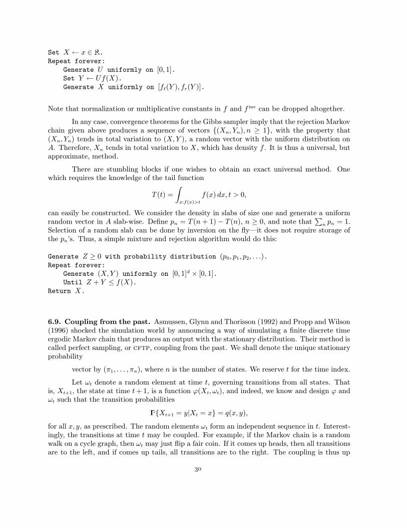
Set X ← x ∈ �.

Repeat forever:

Generate U uniformly on [0, 1].Set Y ← Uf(X).Generate X uniformly on [f`(Y ), fr(Y )].

Note that normalization or multiplicative constants in f and f inv can be dropped altogether.

In any case, convergence theorems for the Gibbs sampler imply that the rejection Markovchain given above produces a sequence of vectors {(Xn, Yn), n ≥ 1}, with the property that(Xn, Yn) tends in total variation to (X,Y ), a random vector with the uniform distribution onA. Therefore, Xn tends in total variation to X, which has density f . It is thus a universal, butapproximate, method.

There are stumbling blocks if one wishes to obtain an exact universal method. Onewhich requires the knowledge of the tail function

T (t) =

∫

x:f(x)>t

f(x) dx, t > 0,

can easily be constructed. We consider the density in slabs of size one and generate a uniformrandom vector in A slab-wise. Define pn = T (n+ 1)− T (n), n ≥ 0, and note that

∑n pn = 1.

Selection of a random slab can be done by inversion on the fly—it does not require storage ofthe pn’s. Thus, a simple mixture and rejection algorithm would do this:

Generate Z ≥ 0 with probability distribution (p0, p1, p2, . . .).Repeat forever:

Generate (X,Y ) uniformly on [0, 1]d × [0, 1].Until Z + Y ≤ f(X).

Return X.

6.9. Coupling from the past. Asmussen, Glynn and Thorisson (1992) and Propp and Wilson(1996) shocked the simulation world by announcing a way of simulating a finite discrete timeergodic Markov chain that produces an output with the stationary distribution. Their method iscalled perfect sampling, or cftp, coupling from the past. We shall denote the unique stationaryprobability

vector by (π1, . . . , πn), where n is the number of states. We reserve t for the time index.

Let ωt denote a random element at time t, governing transitions from all states. Thatis, Xt+1, the state at time t+ 1, is a function ϕ(Xt, ωt), and indeed, we know and design ϕ andωt such that the transition probabilities

� {Xt+1 = y|Xt = x} = q(x, y),

for all x, y, as prescribed. The random elements ωt form an independent sequence in t. Interest-ingly, the transitions at time t may be coupled. For example, if the Markov chain is a randomwalk on a cycle graph, then ωt may just flip a fair coin. If it comes up heads, then all transitionsare to the left, and if comes up tails, all transitions are to the right. The coupling is thus up

to the designer. In the cftp method, the sequence ωt is fixed once and for all, but we need togenerate only a finite number of them, luckily, to run the algorithm.

Pick a positive integer T . A basic run of length T consists of n Markov chains, eachfired up from a different state for T time units, starting at time −T until time 0, using therandom elements ωt,−T ≤ t < 0. This yields n runs Xt(i), 1 ≤ i ≤ n (i denotes the startingpoint), −T ≤ t ≤ 0, with X−T (i) = i. Observe that if two runs collide at a given time t, thenthey will remain together forever. If X0(i) is the same for all i, then all runs have collided. Inthat case, Propp and Wilson showed that X0(.) has the stationary distribution. If there is noagreement among the X0(i)’s, then replace T by 2T and repeat, always doubling the horizonuntil all X0(i)’s agree. Return the first X0(.) for which agreement was observed.

It is interesting that coupling in the future does not work. We cannot simply start the nchains X0(i) = i and let T be the first time when they coalesce, because there are no guaranteesthat XT (.) has the stationary distribution. To see this, consider a directed cycle with n vertices,in which state 1 is the only state with a loop (occurring with probability ε > 0). Coalescencecan only take place at this state, so XT (.) = 1, no matter what. Yet, the limiting distributionis roughly uniform over the states when ε > 0 is small.

The effort needed may be prohibitive, as the time until agreement in a well designedcoupling is roughly related to the mixing time of a Markov chain, so that n times the mixingtime provides a rough bound of the computational complexity. Luckily, we have the freedom todesign the random elements in such a manner that coalescence can be checked without doingn runs. For example, for a random walk on the chain graph with n vertices, where a loop isadded (with probability 1/2) at each state to make the Markov chain aperiodic, we design theωt such that no two paths ever cross. Then coalescence can be checked by following the chainsstarted at states 1 and n only. The coupling in ωt is as follows: draw a uniform integer from{−2,−1, 1, 2}. If it is −2, then all transitions are to the left, except the transition from state 1,which stays. If it is 2, then all transitions are to the right, except the transition from state n,which stays. If it is −1, then all states stay, except state n, which takes a step to the left. If itis 1, then all states stay, except state 1, which takes a step to the right. As the number of stepsuntil the two extreme runs meet is of the order of n2, the expected complexity is also of thatorder. For more on the basics of random walks on graphs and mixing times for Markov chains,see Aldous and Fill (2004).

If the state space is countably infinite or uncountable (say,�d), then special constructions

are needed to make sure that we only have to run finitely many chains, see, e.g., Green andMurdoch (2000), Wilson (2000), Murdoch (2000), or Mira, Moller and Roberts (2001). Mostsolutions assume the existence of a known dominating density g, with f ≤ cg for a constant c,with random samples from g needed to move ahead. The resulting algorithms are still inferiorto the corresponding rejection method, so further research is needed in this direction.

6.10. Further research. If one accepts approximations with density fn of the density f ,where n is the computational complexity of the approximation, then a study must be madethat compares

∫|fn − f | among various methods. For example, fn could be the n-th iterate

in the slice sampler, while a competitor could be gn, the density in the approximate rejectionmethod, which (incorrectly) uses rejection from n (so that gn is proportional to min(f, n), and∫|gn − f | = 2

∫(f − n)+). Both methods have similar complexities (linear in n), but a broad

comparison of the total variation errors is still lacking. In fact, the rejection method could bemade adaptive: whenever an X is generated for which f(X) > n, then replace n by f(X) andcontinue.

Simple exact simulation methods that are based upon iterative non-Markovian schemescould be of interest. Can coupling from the past be extended and simplified?

8. References

J. H. Ahrens, “Sampling from general distributions by suboptimal division of domains,” vol. 19,Grazer Mathematische Berichte, 1993.

J. H. Ahrens, “A one-table method for sampling from continuous and discrete distribu-tions,” Computing, vol. 54, pp. 127–146, 1995.

J. H. Ahrens and U. Dieter, “Computer methods for sampling from gamma, beta, Poisson and bi-nomial distributions,” Computing, vol. 12, pp. 223–246, 1974.

J. H. Ahrens and U. Dieter, “Sampling from binomial and Poisson distributions: a method withbounded computation times,” Computing, vol. 25, pp. 193–208, 1980.

J. H. Ahrens and U. Dieter, “Generating gamma variates by a modified rejection tech-nique,” Communications of the ACM, vol. 25, pp. 47–54, 1982.

J. H. Ahrens and U. Dieter, “An alias method for sampling from the normal distribution,” Com-puting, vol. 42, pp. 159–17159-170, 1989.

J. H. Ahrens and U. Dieter, “A convenient sampling method with bounded computa-tion times for Poisson distributions,” in: The Frontiers of Statistical Computation, Simula-tion and Modeling, (edited by P. R. Nelson, E. J. Dudewicz, A. Ozturk, and E. C. van derMeulen), pp. 137–149, American Sciences Press, Columbus, OH, 1991.

J. H. Ahrens, K. D. Kohrt, and U. Dieter, “Algorithm 599. Sampling from gamma and Pois-son distributions,” ACM Transactions on Mathematical Software, vol. 9, pp. 255–257, 1983.

N. I. Akhiezer, The Classical Moment Problem, Hafner, New York, 1965.

D. Aldous and J. Fill, “Reversible Markov Chains and Random Walks on Graphs,” Manuscriptaavailable at http://128.32.135.2/users/aldous/RWG/book.html, 2004.

S. Asmussen, P. Glynn, and H. Thorisson, “Stationary detection in the initial transient prob-lem,” ACM Transactions on Modeling and Computer Simulation, vol. 2, pp. 130–157, 1992.

R. W. Bailey, “Polar generation of random variates with the t distribution,” Mathemat-ics of Computation, vol. 62, pp. 779–781, 1994.

J. Besag, “On the statistical analysis of dirty pictures (with discussions),” Journal of the RoyalStatistical Society, Series B, pp. 259–302, 1986.

J. Besag and P. J. Green, “Spatial statistics and Bayesian computation,” Journal of the RoyalStatistical Society B, vol. 55, pp. 25–37, 1993.

D. J. Best, “A simple algorithm for the computer generation of random samples from a Stu-dent’s t or symmetric beta distribution,” in: COMPSTAT 1978: Proceedings in Computa-tional Statistics, (edited by L. C. A. Corsten and J. Hermans), pp. 341–347, Physica Ver-lag, Wien, Austria, 1978.

D. J. Best, “Letter to the editor,” Applied Statistics, vol. 27, p. 181, 1978.

D. J. Best, “A note on gamma variate generators with shape parameter less than unity,” Com-puting, vol. 30, pp. 185–188, 1983.

L. Bondesson, “On simulation from infinitely divisible distributions,” Advances in Applied Prob-ability, vol. 14, pp. 855–869, 1982.

G. E. P. Box and M. E. Muller, “A note on the generation of random normal deviates,” An-nals of Mathematical Statistics, vol. 29, pp. 610–611, 1958.

R. E. Caflisch, W. J. Morokoff, and A. B. Owen, “Valuation of mortgage backed securi-ties using Brownian bridges to reduce effective dimension,” Journal of Computational Fi-nance, vol. 1, pp. 27–46, 1997.

J. M. Chambers, C. L. Mallows, and B. W. Stuck, “A method for simulating stable random vari-ables,” Journal of the American Statistical Association, vol. 71, pp. 340–344, 1976.

R. C. H. Cheng, “The generation of gamma variables with non-integral shape parameter,” Ap-plied Statistics, vol. 26, pp. 71–75, 1977.

R. C. H. Cheng and G. M. Feast, “Some simple gamma variate generators,” Applied Statis-tics, vol. 28, pp. 290–295, 1979.

R. C. H. Cheng and G. M. Feast, “Gamma variate generators with increased shape parame-ter range,” Communications of the ACM, vol. 23, pp. 389–393, 1980.

H. C. Chen and Y. Asau, “On generating random variates from an empirical distribu-tion,” AIIE Transactions, vol. 6, pp. 163–166, 1974.

L. Devroye, “The series method in random variate generation and its application to theKolmogorov-Smirnov distribution,” American Journal of Mathematical and Management Sci-ences, vol. 1, pp. 359–379, 1981a.

L. Devroye, “The computer generation of random variables with a given characteristic func-tion,” Computers and Mathematics with Applications, vol. 7, pp. 547–552, 1981b.

L. Devroye, “The computer generation of Poisson random variables,” Computing, vol. 26,pp. 197–207, 1981c.

L. Devroye, “Methods for generating random variates with Polya characteristic functions,”Statistics and Probability Letters, vol. 2, pp. 257–261, 1984a.

L. Devroye, “Random variate generation for unimodal and monotone densities,” Comput-ing, vol. 32, pp. 43–68, 1984b.

L. Devroye, “A simple algorithm for generating random variates with a log-concave den-sity,” Computing, vol. 33, pp. 247–257, 1984c.

L. Devroye, Non-Uniform Random Variate Generation, Springer-Verlag, New York, 1986a.

L. Devroye, “An automatic method for generating random variables with a given characteris-tic function,” SIAM Journal of Applied Mathematics, vol. 46, pp. 698–719, 1986b.

L. Devroye, “The analysis of some algorithms for generating random variates with a given haz-ard rate,” Naval Research Logistics Quarterly, vol. 33, pp. 281–292, 1986c.

L. Devroye, “A simple generator for discrete log-concave distributions,” Computing, vol. 39,pp. 87–91, 1987a.

L. Devroye, A Course in Density Estimation, Birkhauser, Boston, 1987b.

L. Devroye, “Generating sums in constant average time,” in: Proceedings of the 1988 Win-ter Simulation Conference, (edited by M. A. Abrams, P. L. Haigh and J. C. Comfort), pp. 425–431, IEEE, San Diego, CA., 1988.

L. Devroye, “On random variate generation when only moments or Fourier coefficients areknown,” Mathematics and Computers in Simulation, vol. 31, pp. 71–89, 1989.

L. Devroye, “A note on Linnik’s distribution,” Statistics and Probability Letters, vol. 9, pp. 305–306, 1990.

L. Devroye, “Algorithms for generating discrete random variables with a given generating func-tion or a given moment sequence,” SIAM Journal on Scientific and Statistical Comput-ing, vol. 12, pp. 107–126, 1991.

L. Devroye, “Random variate generation in one line of code,” in: 1996 Winter Simulation Con-ference Proceedings, (edited by J. M. Charnes, D. J. Morrice, D. T. Brunner and J. J. Swain),pp. 265–272, ACM, San Diego, CA, 1996.

L. Devroye, “Simulating theta random variates,” Statistics and Probability Letters, vol. 31,pp. 2785–2791, 1997.

L. Devroye, J. Fill, and R. Neininger, “Perfect simulation from the quicksort limit distribu-tion,” Electronic Communications in Probability, vol. 5, pp. 95–99, 2000.

L. Devroye, “Simulating perpetuities,” Methodologies and Computing in Applied Probabil-ity, vol. 3, pp. 97–115, 2001.

L. Devroye and R. Neininger, “Density approximation and exact simulation of random vari-ables that are solutions of fixed-point equations,” Advances of Applied Probability, vol. 34,pp. 441–468, 2002.

K. Dickman, “On the frequency of numbers containing prime factors of a certain magni-tude,” Arkiv for Mathematik, Astronomi oc Fysik, vol. 22A, p. 1014, 1930.

D. Dugue and M. Girault, “Fonctions convexes de Polya,” Publications de l’Institut de Statis-tique des Universites de Paris, vol. 4, pp. 3–10, 1955.

M. Evans and T. Swartz, “Random variable generation using concavity properties of trans-formed densities,” Journal of Computational and Graphical Statistics, vol. 7, pp. 514–528, 1996.

M. Evans and T. Swartz, Approximating Integrals Via Monte Carlo and Deterministic Meth-ods, Oxford University Press, Oxford, UK, 2000.

W. Feller, “On the Kolmogorov-Smirnov limit theorems for empirical distributions,” An-nals of Mathematical Statistics, vol. 19, pp. 177–189, 1948.

J. Fill, “An interruptible algorithm for perfect sampling via Markov chains,” The Annals of Ap-plied Probability, vol. 8, pp. 131–162, 1998.

P. Flajolet and N. Saheb, “The complexity of generating an exponentially distributed vari-ate,” Journal of Algorithms, vol. 7, pp. 463–488, 1986.

B. L. Fox, Strategies for Quasi-Monte Carlo, Kluwer Academic Publishers, Boston, 1999.

A. E. Gelfand and A. F. M. Smith, “Sampling-based approaches to calculating marginal densi-ties,” Journal of the American Statistical Association, vol. 85, pp. 398–409, 1990.

S. Geman and D. Geman, “Stochastic relaxation, Gibbs distributions, and the Bayesian restora-tion of images,” IEEE Transactions on Pattern Analysis and Machine Intelligence, vol. 6,pp. 721–741, 1984.

S. Geman and D. McClure, “Bayesian image analysis: An application to single photon emis-sion tomography,” in: Proceedings of the Statistical Computing Section, pp. 12–18, Washing-ton, DC, 1985.

W. R. Gilks and P. Wild, “Adaptive rejection for Gibbs sampling,” Applied Statistics, vol. 41,pp. 337–348, 1992.

W. R. Gilks, N. G. Best, and K. K. C. Tan, “Adaptive rejection Metropolis sampling,” Ap-plied Statistics, vol. 41, pp. 337–348, 1995.

C. M. Goldie and R. Grubel, “Perpetuities with thin tails,” Advances in Applied Probabil-ity, vol. 28, pp. 463–480, 1996.

P. J. Green and D. J. Murdoch, “Exact sampling for Bayesian inference: towards general pur-pose algorithms (with discussion),” in: Monte Carlo Methods, (edited by J. M. Bernardo,J. O. Berger, A. P. Dawid, and A. F. M. Smith), pp. 301–321, Bayesian Statistics, vol. 6, Ox-ford university Press, Oxford, 2000.

O. Haggstrom, Finite Markov Chains and Algorithmic Applications, Cambridge Univer-sity Press, Cambridge, UK, 2002.

W. Hastings, “Monte Carlo sampling methods using Markov chains and their applica-tions,” Biometrika, vol. 57, pp. 97-110, 1970.

L. Holden, “Geometric convergence of the Metropolis-Hastings simulation algorithm,” Statis-tics and Probability Letters, vol. 39, pp. 371–377, 1998.

W. Hormann, “The generation of binomial random variates,” Journal of Statistical Computa-tion and Simulation, vol. 46, pp. 101–110, 1993a.

W. Hormann, “The transformed rejection method for generating Poisson random variables,” In-surance: Mathematics and Economics, vol. 12, pp. 39–45, 1993b.

W. Hormann, “A universal generator for discrete log-concave distributions,” Computing, vol. 52,pp. 89–96, 1994.

W. Hormann and G. Derflinger, “Universal generators for correlation induction,” in: COMP-STAT 94, (edited by R. Dutter and W. Grossmann), pp. 52–57, Physica-Verlag, Heidel-berg, 1994.

W. Hormann, “A rejection technique for sampling from T-concave distributions,” ACM Trans-actions on Mathematical Software, vol. 21, pp. 182–193, 1995.

W. Hormann, J. Leydold, and G. Derflinger, Automatic Nonuniform Random Variate Genera-tion, Springer-Verlag, Berlin, 2004.

D. Huffman, “A method for the construction of minimum-redundancy codes,” Proceed-ings of the IRE, vol. 40, pp. 1098–1101, 1952.

D. Jackson, “The Theory of Approximation,” Colloquia Publications, vol. 11, American Math-ematical Society, Providence, RI, 1930.

S. F. Jarner and E. Hansen, “Geometric ergodicity of Metropolis algorithms,” Depart-ment of Statistics, University of Copenhagen, 1998.

N. L. Johnson and S. Kotz, Distributions in Statistics: Discrete Distributions, John Wi-ley, New York, N.Y., 1969.

V. Kachitvichyanukul and B. W. Schmeiser, “Binomial random variate generation,” Communi-cations of the ACM, vol. 31, pp. 216–222, 1988.

V. Kachitvichyanukul and B. W. Schmeiser, “Algorithm 678: BTPEC: sampling from the bino-mial distribution,” ACM Transactions on Mathematical Software, vol. 15, pp. 394–397, 1989.

M. Kanter, “Stable densities under change of scale and total variation inequalities,” An-nals of Probability, vol. 3, pp. 697–707, 1975.

M. S. Keane and G. L. O’Brien, “A Bernoulli factory,” ACM Transactions on Modeling and Com-puter Simulation, vol. 4, pp. 213–219, 1994.

D. E. Knuth and A. C. Yao, “The complexity of nonuniform random number generation,” in: Al-gorithms and Complexity, (edited by J. E. Traub), pp. 357–428, Academic Press, New York,N.Y., 1976.

S. Kotz and I. V. Ostrovskii, “A mixture representation of the Linnik distribution,” Statis-tics and Probability Letters, vol. 26, pp. 61–64, 1996.

M. G. Krein, “On one extrapolation problem of A.N. Kolmogorov,” Dokl. Akad. Nauk SSSR,vol. 46, pp. 339–342, 1944.

R. G. Laha, “On a class of unimodal distributions,” Proceedings of the American Mathemati-cal Society, vol. 12, pp. 181–184, 1961.

D. Le Minh, “Generating gamma variates,” ACM Transactions on Mathematical Software,vol. 14, pp. 261–266, 1988.

G. Letac, “On building random variables of a given distribution,” Annals of Probabil-ity, vol. 3, pp. 298–306, 1975.

P. A. W. Lewis and G. S. Shedler, “Simulation of nonhomogeneous Poisson processes by thin-ning,” Naval Research Logistics Quarterly, vol. 26, pp. 403–413, 1979.

J. Leydold, “Automatic sampling with the ratio-of-uniforms method,” ACM Transactions onMathematical Software, vol. 26, pp. 78–98, 2000a.

J. Leydold, “A note on transformed density rejection,” Computing, vol. 65, pp. 187–192, 2000b.

J. Leydold, “A simple universal generator for continuous and discrete univariate T-concave dis-tributions,” ACM Transactions on Mathematical Software, vol. 27, pp. 66–82, 2001.

G. D. Lin, “On the moment problem,” Statistics and Probability Letters, vol. 35, pp. 85–90, 1997.

Yu. V. Linnik, “Linear forms and statistical criteria,I,II,” Selected Translations in Mathemati-cal Statistics and Probability, vol. 3, pp. 1–90, 1962.

J. S. Liu, “Metropolized independent sampling with comparisons to rejection sampling and im-portance sampling,” Statistics and Computing, vol. 6, pp. 113–119, 1996.

G. Marsaglia and W. W. Tsang, “A simple method for generating gamma variables,” ACMTransactions on Mathematical Software , vol. 24, pp. 341–350, 2001.

G. Marsaglia, M. D. Maclaren, and T. A. Bray, “A fast procedure for generating normal ran-dom variables,” Communications of the ACM, vol. 7, pp. 4–10, 1964.

G. Marsaglia, “The squeeze method for generating gamma variates,” Computers and Mathe-matics with Applications, vol. 3, pp. 321–325, 1977.

G. Marsaglia and W. W. Tsang, “A fast, easily implemented method for sampling from decreas-ing or symmetric unimodal density functions,” SIAM Journal on Scientific and Statistical Com-puting, vol. 5, pp. 349–359, 1984.

N. Metropolis, A. Rosenbluth, M. Rosenbluth, A. Teller, and E. Teller, “Equations of state cal-culations by fast computing machines,” Journal of Chemical. Physics, vol. 21, p. 10871091, 1953.

S. P. Meyn and R. L. Tweedie, Markov Chains and Stochastic Stability, Springer-Verlag, Lion-don, 1993.

A. Mira, J. Moller, and G. O. Roberts, “Perfect slice samplers,” Journal of the Royal Statisti-cal Society B, vol. 63, pp. 593–606, 2001.

D. J. Murdoch, “Exact sampling for Bayesian inference: unbounded state spaces,” in: MonteCarlo Methods, (edited by N. Madras), pp. 111–121, Fields Institute Communications, vol. 6,American Mathematical Society, 2000.

R. B. Nelsen, An Introduction to Copulas , Springer-Verlag, Berlin, 1999.

J. G. Propp and D. B. Wilson, “Exact sampling with coupled Markov chains and applica-tions to statistical mechanics,” Random Structures and Algorithms, vol. 9, pp. 223–252, 1996.

S. T. Rachev, Probability Metrics and the Stability of Stochastic Models, John Wiley, NewYork, 1991.

A. Renyi and G. Szekeres, “On the height of trees,” Journal of the Australian Mathematical So-ciety, vol. 7, pp. 497–507, 1967.

U. Rosler and L. Ruschendorf, “The contraction method for recursive algorithms,” Algorith-mica, vol. 29, pp. 3–33, 2001.

K. Sato, Levy Processes and Infinitely Divisible Distributions, Cambridge University Press,Cambridge, 2000.

H. Scheffe, “A useful convergence theorem for probability distributions,” Annals of Mathemat-ical Statistics, vol. 18, pp. 434–458, 1947.

B. W. Schmeiser and A. J. G. Babu, “Beta variate generation via exponential majorizing func-tions,” Operations Research, vol. 28, pp. 917–926, 1980.

B. W. Schmeiser and R. Lal, “Squeeze methods for generating gamma variates,” Jour-nal of the American Statistical Association, vol. 75, pp. 679–682, 1980.

E. Stadlober, “Sampling from Poisson, binomial and hypergeometric distributions: ratio of uni-forms as a simple fast alternative,” Habilitationsschrift, Institute of Statistics, Technical Uni-versity of Graz, Austria, 1988.

E. Stadlober, “Binomial random variate generation: a method based on ratio of uniforms,” Amer-ican Journal of Mathematical and Management Sciences, vol. 9, pp. 1–20, 1989.

E. Stadlober, “The ratio of uniforms approach for generating discrete random variates,” Jour-nal of Computational and Applied Mathematics, vol. 31, pp. 181–189, 1990.

J. Stoyanov, “Krein condition in probabilistic moment problems,” Bernoulli, vol. 6, pp. 939–949, 2000.

R. Swendsen and J. Wang, “Non-universal critical dynamics in Monte Carlo simulation,” Phys-ical review Letters, vol. 58, pp. 86–88, 1987.

L. Tierney, “Markov chains for exploring posterior distributions,” Annals of Statistics, vol. 22,pp. 1701–1762, 1994.

G. Ulrich, “Computer generation of distributions on the m-sphere,” Applied Statistics, vol. 33,pp. 158–163, 1984.

W. Vervaat, “On a stochastic difference equation and a representation of non-negative in-finitely divisible random variables,” Advances in Applied Probability, vol. 11, pp. 750–783, 1979.

J. von Neumann, “Various techniques used in connection with random digits,” CollectedWorks, vol. 5, pp. 768–770, Pergamon Press, 1963. also: in Monte Carlo Method, National Bu-reau of Standards Series, Vol. 12, pp. 36-38, 1951.

A. J. Walker, “New fast method for generating discrete random numbers with arbitrary fre-quency distributions,” Electronics Letters, vol. 10, pp. 127–128, 1974.

A. J. Walker, “An efficient method for generating discrete random variables with general dis-tributions,” ACM Transactions on Mathematical Software, vol. 3, pp. 253–256, 1977.

R. L. Wheeden and A. Zygmund, Measure and Integral, Marcel Dekker, New York, N.Y., 1977.

D. B. Wilson, “Layered multishift coupling for use in perfect sampling algorithms (with a primeron CFTP),” in: Monte Carlo Methods, (edited by N. Madras), pp. 141–176, Fields Institute Com-munications, vol. 6, American Mathematical Society, 2000.

H. Zechner and E. Stadlober, “Generating beta variates via patchwork rejection,” Comput-ing, vol. 50, pp. 1–18, 1993.

V. M. Zolotarev, “On analytic properties of stable distribution laws,” Selected Transla-tions in Mathematical Statistics and Probability, vol. 1, pp. 207–211, 1959.

V. M. Zolotarev, “On the representation of stable laws by integrals,” Selected Transla-tions in Mathematical Statistics and Probability, vol. 6, pp. 84–88, 1966.

V. M. Zolotarev, “Integral transformations of distributions and estimates of parameters of mul-tidimensional spherically symmetric stable laws,” in: Contributions to Probability, pp. 283–305, Academic Press, 1981.

V. M. Zolotarev, One-Dimensional Stable Distributions, American Mathematical Society, Prov-idence, R.I., 1986.