Generating Random Variates

• Use Trace Driven Simulations

• Use Empirical Distributions

• Use Parametric Distributions

Ref: L. Devroye Non-Uniform Random Variate Generation

Trace-driven Simulations

+ Strong validity argument+ Easy to model systems- Expensive- Validity (data representative?)- Sensitivity analysis difficult- Results cannot be generalized to other systems

(restrictive)- Slow- No rare data information

Empirical Distributions (histograms)

+ Strong validity argument+ Easy to model systems+ Replicate- Data may not be representative- Sensitivity analysis is difficult- Results cannot be generalized to other systems- Difficult to model dependent data- Need a lot of data (must do conditional sampling)- Outliers and rare data problems

Parametric Probability Model

+ Results can be generalized

+ Can do sensitivity analysis

+ Replicate

- Data may not be representative

- Probability distribution selection error

- Parametric fitting error

Random Variate Generation:General Methods

• Inverse Transform

• Composition

• Acceptance/Rejection

• Special Properties

Criteria for Comparing Algorithms

• Mathematical validity – does it give what it is supposed to?

• Numerical stability – do some “seeds” cause problems?

• Speed• Memory requirements – are they excessively

large?• Implementation (portability)• Parametric stability – is it uniformly fast for all

input parameters (e.g. will it take longer to generate PP as rate increases?)

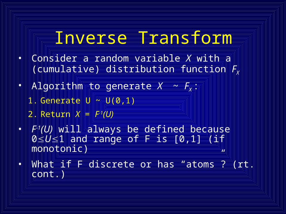
Inverse Transform• Consider a random variable X with a (cumulative)

distribution function FX

• Algorithm to generate X ~ FX :

1. Generate U ~ U(0,1)

2. Return X = F-1(U)

• F-1(U) will always be defined because 0U1 and range of F is [0,1] (if monotonic)

• What if F discrete or has “atoms”? (rt. cont.)

Consider discrete random variate, X

-4 21

P{X=k} = Pk

P-4 P1P2

U (0,1)

Random Number, U, falls in interval k with Prob = Pk

Return k corresponding to interval (use an array or table)

0 1

Pk = 1 so lay out Pks along Unit Interval

Equivalent to “inverting” the CDF

x

1

U1

U2

X1=2X2=-4

-4 21

P{X=k}

Fx(k) = Prob{X≤k}

Generating Continuous Random Variates

FX(x)

x

1

U1

U2

X1X2

Proof Algorithm Works• Must show the X generated by the algorithm

is, in fact, from FX : P{X x} = FX(x)

• P{X x} = P{FX-1(U) x} =

P{U FX(x)} = FX(x) = P{X x}

• First equality is conjecture, X = FX-1

(U), second is mult. by Fx (monotone non-dec)

• Note: The = in the conjecture should really be , meaning RVs have same distribution.

defn

defn

e.g. Exponential R.V.

• X is an exponential random variable with mean

• To generate values of X set U = Fx(X) and solve for (rv) X.

X = - ln(1-U) (or X = - ln(U))

otherwise 0

0x if 1 / xexF

Weibull Random Variable (with parameters and )

PDF: f(x) = - x-1 , x0, 0 otherwise

CDF:F(x) = 1- , x0

Setting F(x) = u~U(0,1)

leads to x = (-LN(1-u))1/.

)-(x/e )-(x/e

Triangular Distribution

— Used when a crude, single mode distribution is needed.

2(x-a)/(b-a)(c-a) for a x b

— The PDF is f(x) = 2(c-x)/(c-a)(c-b) for b x c

0 otherwise

where a and c are the boundaries, and b is the mode.

a cb

f(x)

x

— The CDF is F(v) = (v-a)2/(b-a)(c-a) for a v b

1 - (c-v)2/(c-a)(c-b) for b v c

— By the inversion method,

v = a + (u)1/2[(b-a)(c-a)]1/2 for 0 u (b-a)/(c-a)

c - (1-u)1/2[(c-a)(c-b)]1/2 for (b-a)/(c-a) u 1

where F(b) = (b-a)/(c-a)

Geometric Random Variable (with parameter p)

- Number of trials until the first success (with probability p)

- Probability mass function (PMF) P{X=j} = p(1-p) j-1, j=1,2,…

- Cumulative distribution function (CDF)

F(k) = j<k p(1-p) j-1 = 1- (1-p)k

If u = F(k) ~U(0,1), then k = LN(1-u)/(1-p) +1 = LN(1-u)/(1-p).

u = 1- (1-p)k

1- u = (1-p)k

k = LN(1-u)/LN(1-p) (use floor function to discretize)

Inverse Transform: Advantages

• Intuitive

• Can be very fast

• Accurate

• One random variate generated per U(0,1) random number

• Allows variance-reduction techniques to be applied (later)

• Truncation easy

• Order statistics are easy

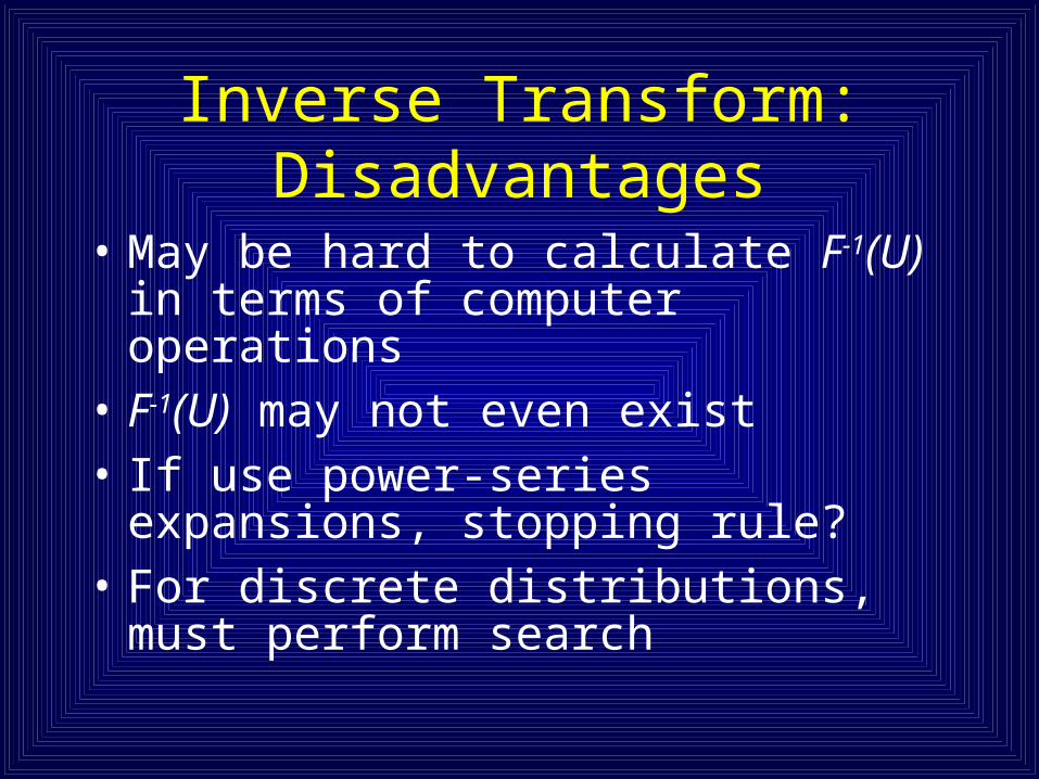
Inverse Transform: Disadvantages

• May be hard to calculate F-1(U) in terms of computer operations

• F-1(U) may not even exist• If use power-series expansions, stopping

rule?• For discrete distributions, must perform

search

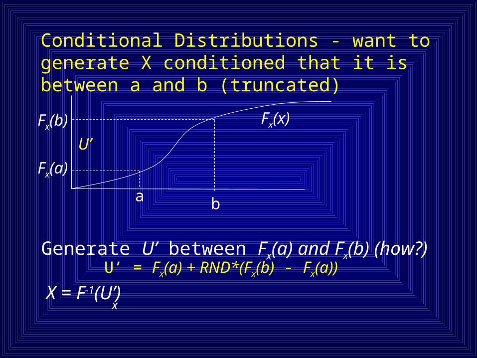
Conditional Distributions - want to generate X conditioned that it is between a and b (truncated)

Fx(x)

a b

Fx(b)

Fx(a)

Generate U’ between Fx(a) and Fx(b) (how?)

X = F-1(U’)x

U’ = Fx(a) + RND*(Fx(b) - Fx(a))

U’

Inverse Transform for Discrete Random Variates

• Inverse transform can be used for discrete random variables, also

• E.g., can use empirical distribution function (see next slide)

• If using known probabilities, replace 1/n step size with p(xi) step size

Variate Generation Techniques: Empirical Distribution

How to sample from a discrete empirical distribution:• Determine {(x1, F(x1)), (x2, F(x2)),…, (xn, F(xn))}• Generate u• Search for interval (F(xi) u F(xi+1))• Report xi

1/n

1

0 x1 x2 x3 xn

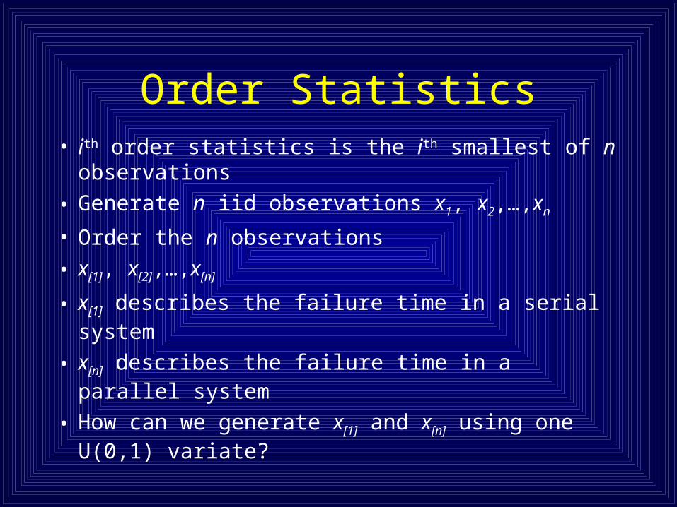
Order Statistics• ith order statistics is the ith smallest of n

observations

• Generate n iid observations x1, x2,…,xn

• Order the n observations

• x[1], x[2],…,x[n]

• x[1] describes the failure time in a serial system

• x[n] describes the failure time in a parallel system

• How can we generate x[1] and x[n] using one U(0,1) variate?

Order Statistics• Serial system

• Parallel system

1 2 n…

n

2

1

…

Order Statistics• F[n](a) = P{x[n]a} = P{Max{xi}a}

= P{x1a, x2a, …, xna}

= P{x1a} P{x2a} … P{xna}(indep)

= Fn(a) (identically distributed)Represents CDF of failure time of parallel

system using CDF of failure time of individual component

• Inversion: Fn(a) = U implies a = F-1((U)1/n)

Order Statistics

• F[1](a) = P{x[1]a} = 1 - P{x[1]>a} =1-P{Min{xi}>a}

= 1 - P{x1>a, x2>a, …, xn>a}

= 1 - P{x1>a} P{x2>a} … P{xn>a}= 1 – (1 - F(a))n

Represents CDF of failure time of serial system using CDF of failure time of individual component

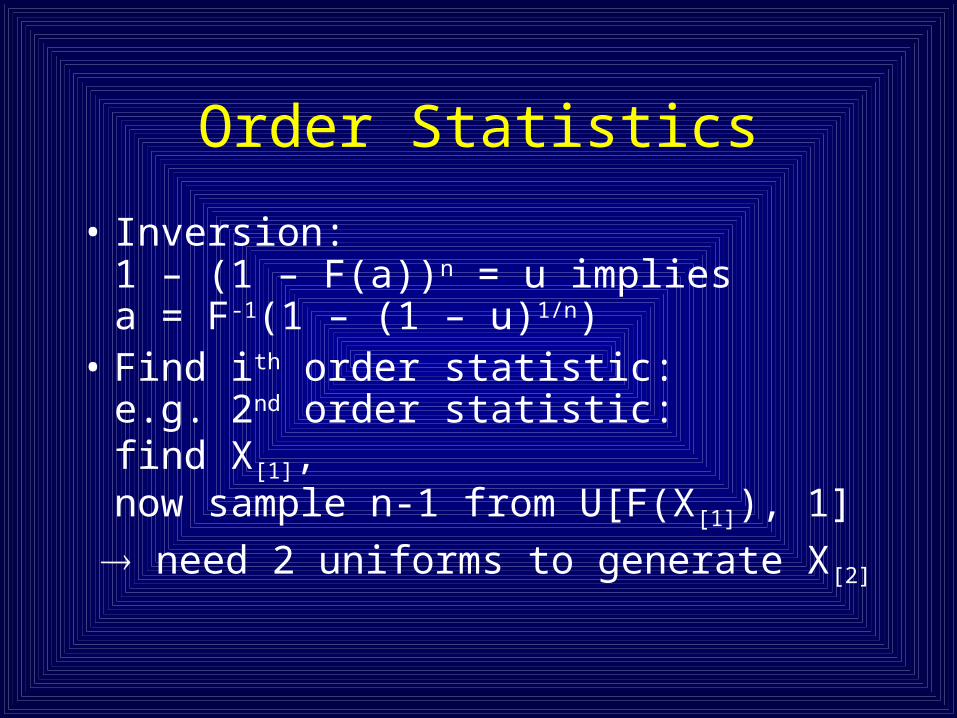
Order Statistics

• Inversion:1 – (1 – F(a))n = u implies a = F-1(1 – (1 – u)1/n)

• Find ith order statistic:e.g. 2nd order statistic: find X[1], now sample n-1 from U[F(X[1]), 1]

need 2 uniforms to generate X[2]

NOTE

— As n+, u1/n 1 and 1 - (1 - u)1/n 0 for u ~ U(0, 1)

— Once the CDF of the order statistics are known, the densities (PDFs) can be obtained by differentiating.

u

0F-1(1-(1-u)1/n) F-1(u) F-1(u1/n) X

F(X)1

U(0,1)

u1/n

1- (1-u)1/n

Example

Let X be exponential with mean = 1/5, and u U(0, 1).

Let n = 100

Then x[100] = (-1/5)1n(1-u1/100) and

x[1] = (-1/5)1n(1 - (1 - (1 - u)1/100)) = (-1/5) 1n((1 -

u)1/100))

For u=.2, x[100] = .827 and x[1] = .0004.For u=.5, x[100] = .995 and x[1] = .0014.For u=.8, x[100] = 1.22 and x[1] = .0032.

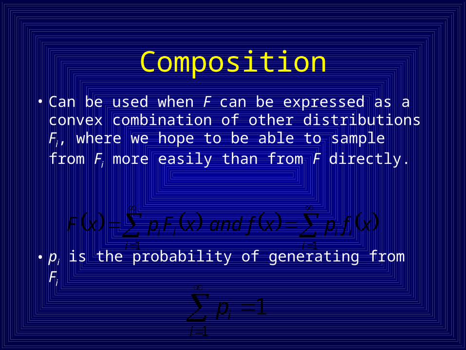
Composition• Can be used when F can be expressed as a

convex combination of other distributions Fi, where we hope to be able to sample from Fi more easily than from F directly.

• pi is the probability of generating from Fi

11 i

iii

ii xfpxf and xFpxF

11

iip

Composition: Graphical Example

f(x)

0.5

0

Area = 0.5 Area = 0.5x

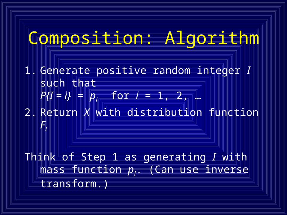
Composition: Algorithm

1. Generate positive random integer I such thatP{I = i} = pi for i = 1, 2, …

2. Return X with distribution function FI

Think of Step 1 as generating I with mass function pI. (Can use inverse transform.)

Composition: Another Example

f(x)

2-a

a

x0 1

Area = a

Area = 1 - a

1. Generate U1

2. If U1 a, generate and return U2

3. Else generate and return X from right-triangular distribution

Acceptance/Rejection

• X has density f(x) with bounded support

• If F is hard (or impossible) to invert, too messy for composition... what to do?

Generate Y from a more manageable distribution and accept as coming from f with a certain probability

x

f(x)

M’(x)

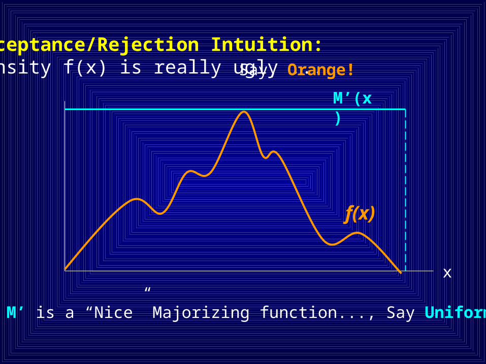
Acceptance/Rejection Intuition:Density f(x) is really ugly ... Say, Orange!

M’ is a “Nice” Majorizing function..., Say Uniform

x

f(x)

M’(x)

Intuition:Throw darts at rectangle under M’ until hit f

X

Reject!Missed again!

Accept X! - done

Proof: Prob{Accept X} is Proportional to height of f(X)

Acceptance/Rejection

• Create majorizing function M(x) f(x) for all x; normalize M( ) to be a density (area=1)

r(x) = M(x)/c where c is the area under M(x)

• Algorithm:1. Generate X from r(x)

2. Generate Y from U(0,M(X)) (independent of X)

3. If Y f(X), Return X; else go to 1 and repeat

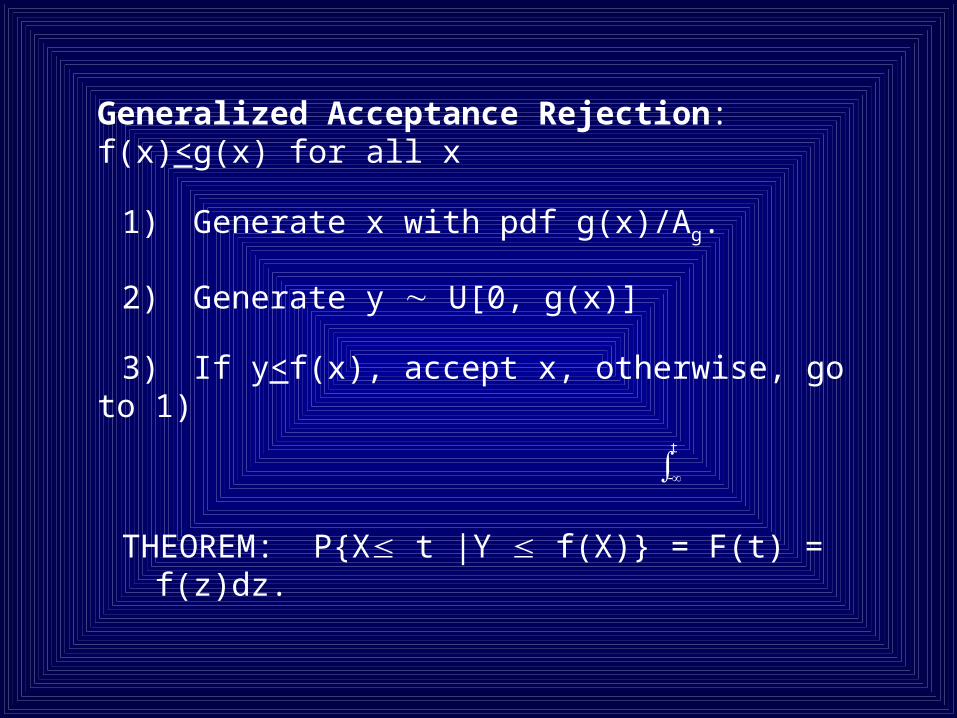
Generalized Acceptance Rejection: f(x)<g(x) for all x

1) Generate x with pdf g(x)/Ag.

2) Generate y U[0, g(x)]

3) If y<f(x), accept x, otherwise, go to 1)

THEOREM: P{X t |Y f(X)} = F(t) = f(z)dz.t

-

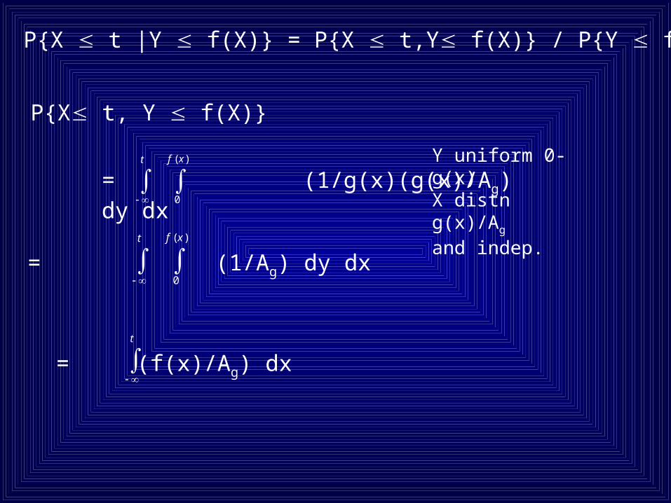
Proof: P{X t |Y f(X)} = P{X t,Y f(X)} / P{Y f(X)}

P{X t, Y f(X)}

= (1/g(x)(g(x)/Ag) dy dx( )

0

f xt

= (1/Ag) dy dx

= (f(x)/Ag) dxt

( )

0

f xt

Y uniform 0-g(x)X distn g(x)/Ag

and indep.

Second,

P{Y f(X)}

= g(x)/(g(x)/Ag) dy dx

( )

0

f x

= (1/Ag) dy dx

= (f(x)/Ag) dx = 1/Ag

( )

0

f x

Therefore, P{X t | Y f(X)} = f(x) dxt

Performance of AlgorithmWill Accept X with a probability equal to

(area under f(X))/ (area under M’(X))

If c = area under M’( ), Probability of acceptance is 1/c – so want c to be small

What is the expected number of U’s needed to generate one X?

2c Why?Each iteration is coin flip (Bernoulli Trial). Number of trials until first success is Geometric, G(p)E[G] = 1/p and here p=1/c (2 Us per iteration)

Increase Prob(accept) and stop with tighter Majorizing Function, M(X)

x

f(x)

M(x)

X

f(X)

f(X)/M(X)

M’(x)

What if f(x) is hard to evaluate?

Use minorizing function m(x) f(x)

f(x)

M(x)

m(x)

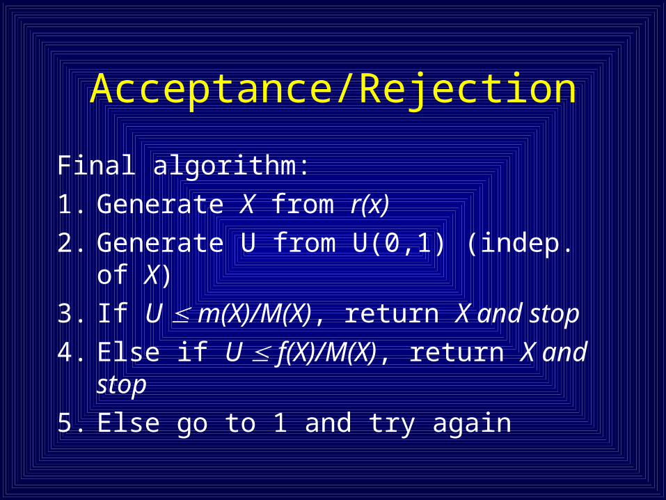
Acceptance/Rejection

Final algorithm:

1. Generate X from r(x)

2. Generate U from U(0,1) (indep. of X)

3. If U m(X)/M(X), return X and stop

4. Else if U f(X)/M(X), return X and stop

5. Else go to 1 and try again

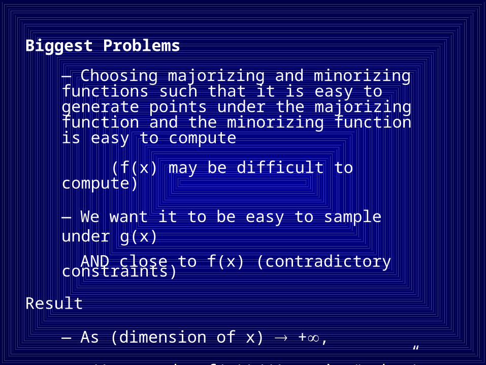
Biggest Problems

— Choosing majorizing and minorizing functions such that it is easy to generate points under the majorizing function and the minorizing function is easy to compute

(f(x) may be difficult to compute)

— We want it to be easy to sample under g(x)

AND close to f(x) (contradictory constraints)

Result

— As (dimension of x) +,

(Area under f(x))/(Area in “cube”) 0

Special Properties

• Methods that make use of “special properties” of distributions to generate them

• E.g. n2 = where Xi is N(0,1)

random variable

• Z1 and Z2 are 2 with k1 and k2 degrees of

freedom, then is Fk1,k2

2

1

n

ii

X

1 1

2 2

/

/

Z kX

Z k

Special Properties

• An Erlang is a sum of exponentials

ERL (r,) =i=1,2,…,r (- 1n(ui)) = - 1n(i=1,2,…,r ui))

(Gamma allows r to be non-negative real)

• If X is Gamma (,1), and Y = X, then Y is Gamma (, ).

If = 1, then X is Exp (1).

• Beta is a ratio of Gammas

X1 is distributed Gamma (1, )

X2 is distributed Gamma (2, )

X1 and X2 are independent

Then X1/(X1+X2) is distributed Beta (1, 2)

Binomial Random Variable Binomial(n,p)

(Bernoulli Approach)

0) X = 0, i = 1

1) Generate U distributed U(0, 1)

2) If U p, X X+1

If U > p, X X

If in, set i i+1 and go to 1)

If i = n, stop with X distributed Binomial (n,p)

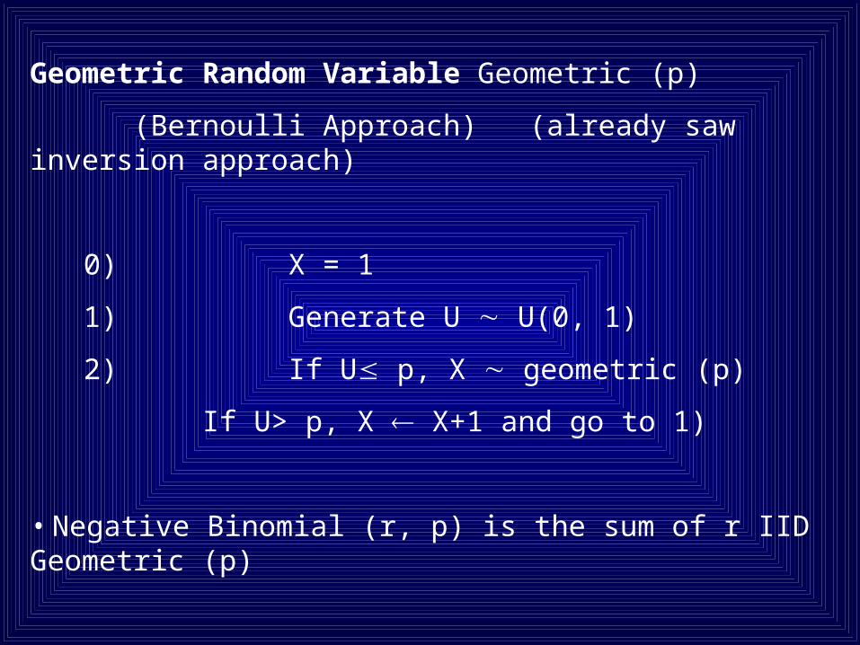
Geometric Random Variable Geometric (p)

(Bernoulli Approach) (already saw inversion approach)

0) X = 1

1) Generate U U(0, 1)

2) If U p, X geometric (p)

If U> p, X X+1 and go to 1)

• Negative Binomial (r, p) is the sum of r IID Geometric (p)

Example of Special Properties:

Poisson RV, P, is sum of exponentials in unit interval

0 1

E[1/] E[1/] E[1/] E[1/]

Has same probability as a Poisson() = 3...

- ln{Ui} ≤ 1 ≤ - ln{Ui} <=> P = kk

i=1

k+1

i=1

Generate E[1/] - ln{Ui} (–L*LN{RND} in sigma)

- ln{Ui} ≤ 1 ≤ - ln{Ui} <=> P = kk

i=1

k+1

i=1

- ln{Ui} ≤ 1 ≤ - ln{ Ui}i=1

k k+1

i=1

ln{Ui} ≥ -1/ ≥ ln{ Ui}i=1

k k+1

i=1

Ui ≥ e-1/ ≥ Uii=1

k k+1

i=1

(log of sum is product of logs)

(multiple by -1/ )

(take exp of everything-monotonic)

Algorithm: to generate Poisson (mean = ), multiplyiid Uniforms (RND) until product is less than e-1/ .

Special Properties:

Assume have Census Data only for Poisson Arrivalseg: Hospitals, Deli Queues, etc.

Use fact that, given K Poisson events occur in T,The Event times are distributed as K Uniforms on (0,T)

First arrival time: Generate T1 = T*U[1:K] = smallest in K Uniforms on (0,T) (min order statistic) = T*(1 – U1/K) (beware of rounding errors on computer)

Next interarrival time = smallest of K-1 Uniforms on (0,T-T1): Generate T2 = (T-T1)*(1 – U1/(K-1))

and so on until get K events in T

Special Properties

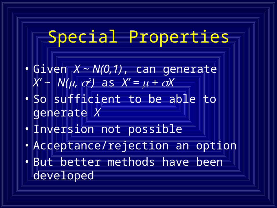
• Given X ~ N(0,1), can generate X’ ~ N(, 2) as X’ = + X

• So sufficient to be able to generate X

• Inversion not possible

• Acceptance/rejection an option

• But better methods have been developed

Normal Random Variables

• Need only generate N(0, 1)

— If X is IID N(0, 1), then Y = X+ is N(,)

1) Crude (Central Limit Theorem) Method

• U U(0, 1), hence E(U) = .5 and V(U) = 1/12.

• Set Y = Ui, hence E(Y) = n/2 and V(Y) = n/12

• By CLT, (Y-n/2)/(n/12)1/2 D N(0, 1) as n +

• Consider Ui-6 (i.e., n = 12).

However n may be too small!

1

n

i

12

1i

Box-Muller Method

• Generate U1, U2 U(0,1) random numbers• Generate

and

• X1 and X2 will be iid N(0,1) random variables

1 1 22ln cos 2X U U

2 1 22ln sin 2X U U

Box-Muller Explanation

• If X1 and X2 iid N(0,1)

• D2 = X12 + X2

2 is 22 which is the SAME as

an Exponential(2)

• X1 = D cos X2 = D sin

where = 2U2

DX2

X1

2lnD U

Polar Method

1. Let U1, U2 be U(0,1),

2. define Vi = 2Ui – 1: Vi is U(-1,1)

3. Define S = V12 + V2

2

4. If S>1, go to 1.

5. If S1, then

1. X1=V1Y and X2=V2Y are iid N(0,1)

2ln SY

S

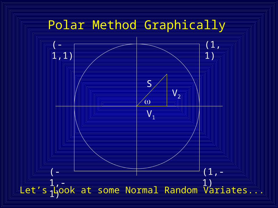
Polar Method Graphically

V1

V2

(-1,-1) (1,-1)

(-1,1)

S

(1,1)

Let’s Look at some Normal Random Variates...

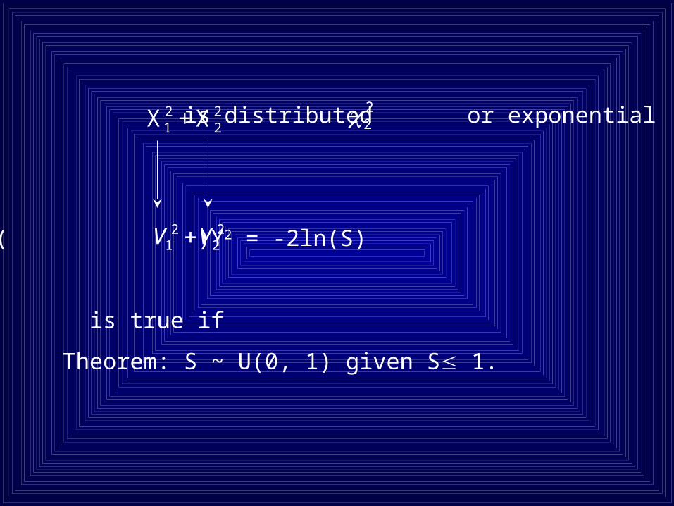
Notes

— is distributed or exponential (2)

or ( )Y2 = -2ln(S)

is true if

Theorem: S ~ U(0, 1) given S 1.

2 21 2X + X

22

2 21 2V V

Proof:

P{S z | S 1} = P{Sz , S1}/ P{S1} = P{Sz }/ P{S1}

= P{ z | S 1}

(since =S) and ( )Y2 = -21n(S))

= P{-(z- )1/2 V1 z- )1/2} / P{S1}

= 1/2 (2/4) (z- )1/2 dV2 / ( /4)

= (zcos2()/2) d/ ( /4) = z

2 21 2V V

2 21 2V V

22V

1/ 2

1/ 2

z

z/ 2

/ 2

2 21 2V V

22V

22V

(later)

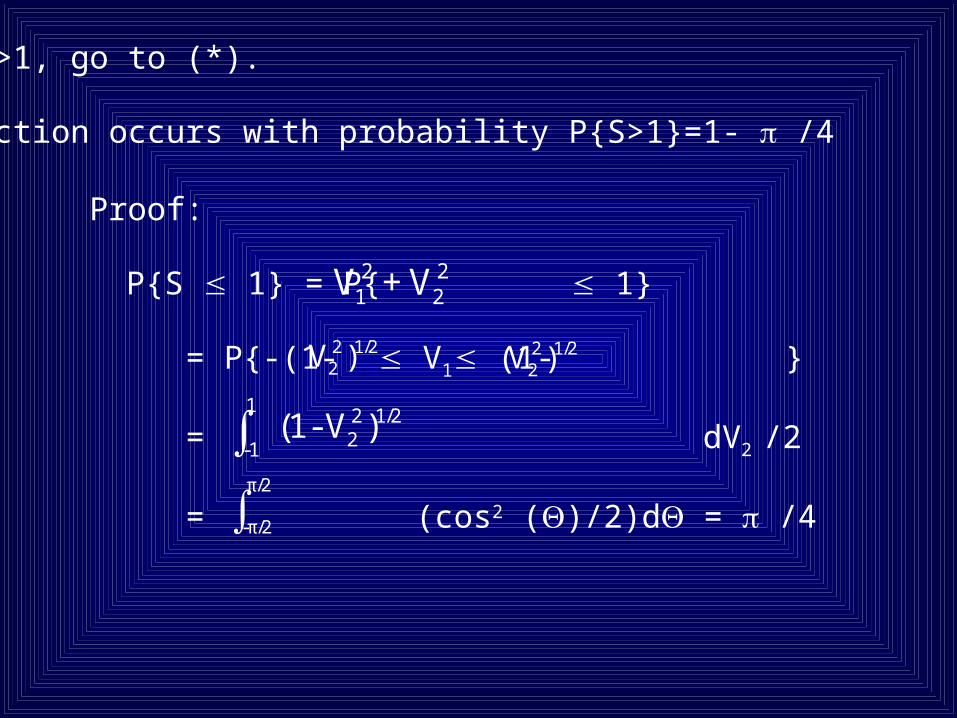
Proof:

P{S 1} = P{ 1}

= P{-(1- V1 (1- }

= dV2 /2

= (cos2 ()/2)d = /4

2 21 2V + V

2 1/22V )

π/2

-π/2

1 2 1/22-1

(1- V )

If S>1, go to (*).

Rejection occurs with probability P{S>1}=1- /4

2 1/22V )

Scatter Plot of X1 and X2 from NOR{} in Sigma

Two successive Normals from Sigma

X1

-418

-260

-102

56

214

372

530

-382 -234 -86 62 210 358 506

X2

Histograms of X1 and X2 from NOR{} in SigmaTwo successive Normals from Sigma

X2

0

108

216

324

432

540

648

-418 -387 -356 -325 -294 -263 -232 -201 -170 -139 -108 -77 -46 -15 16 47 78 109 140 171 202 233 264 295 326 357

Count

Two successive Normals from Sigma

X1

0

103

206

309

412

515

618

-382 -353 -324 -295 -266 -237 -208 -179 -150 -121 -92 -63 -34 -5 24 53 82 111 140 169 198 227 256 285 314 343

Count

Autocorrelations of X1 and X2 from NOR{} in Sigma

Two successive Normals from Sigma

Lag

-1

0

1

0 1 2 3 4 5 6 7 8 9 10

X1

Two successive Normals from Sigma

Lag

-1

0

1

0 1 2 3 4 5 6 7 8 9 10

X2

Histograms of X1 and X2 from Exact Box Muller Algorithm

C:\TEACHING\SIMULA~1\__IEOR~1\BOXMULLR.OUT (X2 Histogram)

X2

0

154

308

462

616

770

924

-247 -227 -207 -187 -167 -147 -127 -107 -87 -67 -47 -27 -7 13 33 53 73 93 113 133 153 173 193 213 233 253

Count

C:\TEACHING\SIMULA~1\__IEOR~1\BOXMULLR.OUT (X1 Histogram)

X1

0

167

334

501

668

835

1002

-296 -274 -252 -230 -208 -186 -164 -142 -120 -98 -76 -54 -32 -10 12 34 56 78 100 122 144 166 188 210 232 254

Count

C:\TEACHING\SIMULA~1\__IEOR~1\BOXMULLR.OUT (Autocorrelations of X1)

Lag

-1

0

1

0 1 2 3 4 5 6 7 8 9 10

X1

C:\TEACHING\SIMULA~1\__IEOR~1\BOXMULLR.OUT (Autocorrelations of X2)

Lag

-1

0

1

0 1 2 3 4 5 6 7 8 9 10

X2

Autocorrelations of X1 and X2 - Exact Box Muller Algorithm

BOXMULLR.OUT (X2 vs. X1)

X1

-247

-144

-41

62

165

268

371

-296 -183 -70 43 156 269 382

X2

Scatter plot of X1 and X2 - Exact Box Muller Algorithm

This is weird! WHY? – Marsaglia’s Theorem in polar coordinates

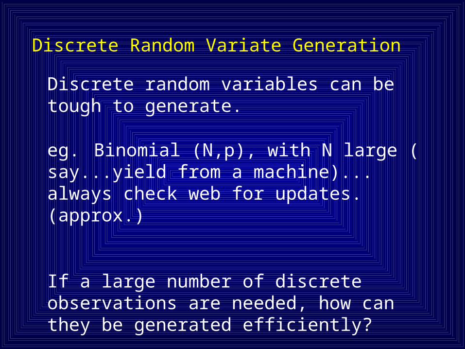
Discrete random variables can be tough to generate.

eg. Binomial (N,p), with N large ( say...yield from a machine)... always check web for updates. (approx.)

If a large number of discrete observations are needed, how can they be generated efficiently?

Discrete Random Variate Generation

Discrete Random Variate Generation

• Crude method: Inversion Requires searching (sort mass function first)

• Continuous approximation e.g. “Geometric is the greatest integer <

Exponential”

• Alias method, ref: Kromal & Peterson, Statistical Computing 33.4, pp.214-218

Alias Method

• Use when

— there are a large number of discrete values.

— you want to generate many variates from this distribution.

• Requires only one U(0, 1) variate.

• Transforms a discrete random variable into a discrete uniform random variable with aliases at each value

(using conditional probability).

Example:

p1 = .2 p2 = .4 p3 = .35 p4 = .05

If uniform, pi = .25 for i = 1, 2, 3, 4

.25

1 2 3 4

.25

Define Qi = probability that i is actually chosen given that i is first selected

= P{i chosen | i selected}

Ai is where to move (alias) to if i is not chosen

1

.25

1 2 3 4

23

4

322

A1 = 2 A2 = 3 A3 = 3 A4 = 2Q1 = .8 Q2 = .6 Q3 = 1. Q4 = .2

Qi = probability that i is actually chosen given that i is first selected

= P{i chosen | i selected}

Ai is where to move (alias) to if i is not chosen

Other Possible Alias Combinations

A1 = 3 A2 = 2 A3 = 2 A4 = 3Q1 = .8 Q2 = 1. Q1 = .4 Q2 = .2

A1 = 3 A2 = 3 A3 = 3 A4 = 2Q1 = .8 Q2 = .8 Q1 = 1. Q2 = .2

0. .2 .25 .4 .50 .75 .80 1.0

1 2 2 3 3 4 2

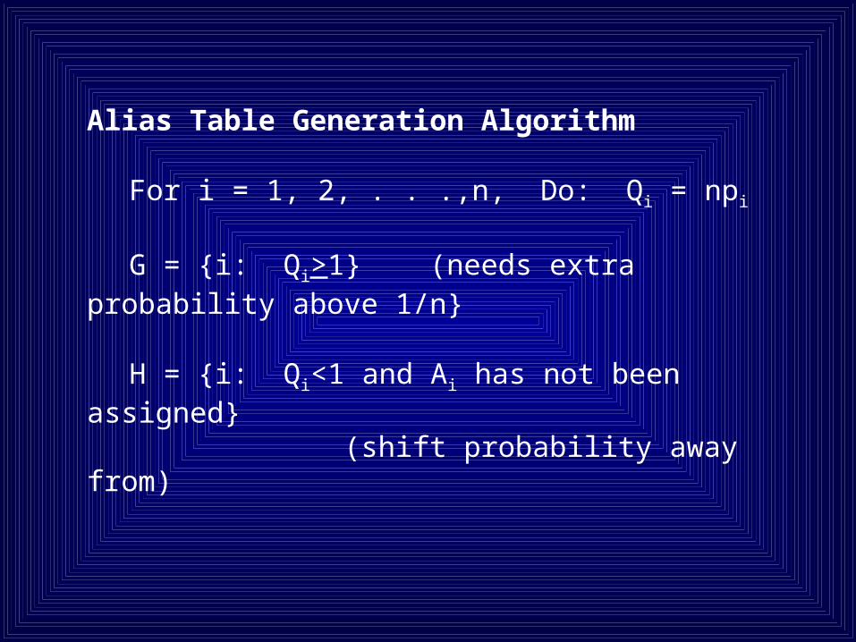
Alias Table Generation Algorithm

For i = 1, 2, . . .,n, Do: Qi = npi

G = {i: Qi>1} (needs extra probability above 1/n}

H = {i: Qi<1 and Ai has not been assigned}(shift probability away from)

While H is nonempty Do:

j: any member of H

k: any member of G

Aj = k

Qk = Qk - (1-Qj)

If Qk <1 then:

G = G\{k}

H = H{k}

end

H = H\{j}

end

Example

i: 1 2 3 4 5pi: .210 .278 .089 .189 .234

Qi: 1.050 1.390 .445 .945 1.170

G X X XH X X

j = 3, k = 1i: 1 2 3 4 5pi: .210 .278 .089 .189 .234

Qi: .495 1.390 .445 .945 1.170

G X XH X XAi 1

j = 1, k =2i: 1 2 3 4 5pi: .210 .278 .089 .189 .234

Qi: .495 .885 .445 .945 1.170

G XH X XAi 2 1

j = 2, k = 5i: 1 2 3 4 5pi: .210 .278 .089 .189 .234

Qi: .495 .885 .445 .945 1.055

G XH XAi 2 5 1

j = 4, k =5i: 1 2 3 4 5pi: .210 .278 .089 .189 .234

Qi: .495 .885 .445 .945 1.000

G XHAi 2 5 1 5

To verify that the table is correct, use

P{i chosen} = P{i chosen | j selected} P{j selected}

= (Qi/n) + (1-Qj)(1/n)j i

p1 = (1/5) (.495 +.555) = .210

p2 = (1/5) (.885 +.505) = .278

p3 = (1/5) (.445) = .089

p4 = (1/5) (.945) = .189

p5 = (1/5) (1.000 +.115 + .055) = .234

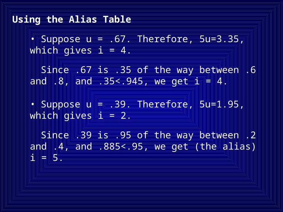
Using the Alias Table

• Suppose u = .67. Therefore, 5u=3.35, which gives i = 4.

Since .67 is .35 of the way between .6 and .8, and .35<.945, we get i = 4.

• Suppose u = .39. Therefore, 5u=1.95, which gives i = 2.

Since .39 is .95 of the way between .2 and .4, and .885<.95, we get (the alias) i = 5.

Marsaglia Tables

• For discrete random variables

• Must have probabilities with denominator as a power of 2

• Use when

— there are a large number of discrete values(shifts work from n values to log2 (n) values)

— you want to generate many values from this distribution

• Requires 2 U(0, 1) variates (actually only need one)

Example

Prob. Binary .5 .25 .125 .0625 .03125

p0=7/32 .00111 x x x

p1=10/32 .01010 x x

p2=10/32 .01010 x x

p3=3/32 .00011 x x

p4=2/32 .00010 x

qi .5 .125 .3125 .0625

Algorithm:

1) pick an urn with probability qi

2) pick a value from the urn with discrete uniform

NOTE: At most log2 (n) values of qi needed (= #columns).

Check with Law of Total Probability:

p0 = 0 +(.125)(1) + (.3125)(1/5) + (.0625)(1/2) = 7/32

p1 = (.5)(1/2) 0 + (.3125)(1/5) +0 = 10/32

p2 = (.5)(1/2) 0 + (.3125)(1/5) +0 = 10/32

p3 = 0 +0 + (.3125)(1/5) + (.0625)(1/2) = 3/32

p4 = 0 +0 + (.3125)(1/5) +0 = 2/32

Poisson Process

Key: times between arrivals are exponentially distributed

N(t)

0t

3

2

1

4

E(1/)

E(1/)E(1/)E(1/) E(1/)

Nonhomogeneous PP

• Rate no longer constant: (t), with distribution

• Tempting: time between ti+1 and ti exponentially distributed with rate (ti)

• BAD IDEA

0

t

t y dy

Nonhomogeneous PP

(t)

tti

Generating at rate (ti) might cause arrival during closed period!

NHPP

(t)

t

Use thinning – same idea as acceptance/rejection:

1. Generate from PP with rate max

2. Accept with probability (t)/max max

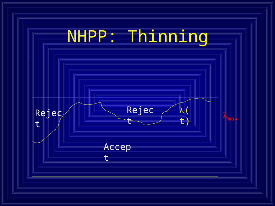
NHPP: Thinning

max

(t)

Accept

RejectReject

exp(m)

m = max (t)

t

m(t)

0

t

* Generate a homogeneous Poisson process with rate m.

* Accept arrivals with probability (t)/m

Inhomogeneous Poisson Process (Thinning)

AcceptReject

see Sigma model NONPOIS.MOD

NHPP: Inversion

t

(t)

Exp(1)

What about fact we don’t really know (t)?

Generating Dependent Data

• Many ways to generate dependent data

• AR(p) process: autoregressive process:Yt = a1Yt-1 + a2Yt-2 + … + apYt-p + t

• MA(q) process: moving average process:Yt = t + b1t-1 + … + bqt-q

• EAR process: exponential autoregressive:Yt = R*Yt-1 + M*ERL{1}*(RND>R)

Autocorrelation

AR(1) autocorrelation lag k = k

Satisfies 1st order difference equn

k = α k-1 k>0

with boundary condition 0=1

Soln: k = αk

EAR Process

• EAR_Q.MOD

• Histograms of the interarrival and service times will appear exponentially distributed.

• Plots of the values over time will look very different

• Output from the model will be very different as R is varied

demo earQ.MOD

Driving Processes

Problem: Real World Stochastic Processes are not independent nor identically distributed...not even stationary.

• Serial Dependencies: yield drift

• Spikes: hard and soft failures

• Cross Dependencies: maintenance

• Nonstationarity – trends, cycles (rush hours)

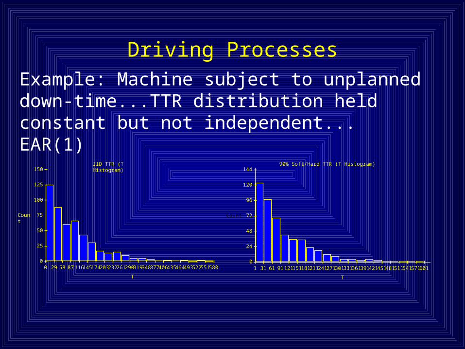
Driving ProcessesExample: Machine subject to unplanned down-time...TTR distribution held constant but not independent... EAR(1)

IID TTR (T Histogram)

T

0

25

50

75

100

125

150

0 29 58 87 116145174203232261290319348377406435464493522551580

Count Count

90% Soft/Hard TTR (T Histogram)

T

0

24

48

72

96

120

144

1 31 61 91 121151181211241271301331361391421451481511541571601

Driving Processes

Example: WIP Charts

iid TTR (WIP vs. Time)

Time

0

50

100

150

200

250

0 10000 20000 30000 40000 50000

WIP

aveW=4.990% SOFT/HARD TTR (WIP vs. Time)

Time

0

50

100

150

200

250

0 20000 40000 60000 80000 100000

WIP

aveW=44.3

Ref: Edward McKenzie "Time Series Analysis in Water Resources" in Water Resources Bulletin; 21.4 pp. 645-650.

Motivation: wish to model realistic situation where random process has serial correlation. This is different from time-dependency (say, for modeling rush-hour traffic) in that value of process depends on its own history, maybe in addition to being dependent on its index (time).

Criteria: (P.A.W.Lewis: Multivariate Analysis - V. (pp: 151-166) North Holland)1. Models specified by marginal distributions and correlation structure.

2. Few parameters that can be easily interpreted.

3. Structure is linear in parameters, making them easy to fit and generate

Models for Dependent Discrete-Valued Processes

AR(order 1) (Markov Models)

Continuous Autoregressive order-1 sequence, {Xn} satisfies the difference equation

(Xn-) = α(Xn-1- ) + n or remove means

Xn = αXn-1 + n with {n} being a sequence of iid random variables and α is a

positive fraction...process retains fraction, α, of previous value.

Note: If Xn is discrete then n must be dependent on Xn-1 ...want to reduce Xn-1 by the "right" amount to have same distn.

Models for Dependent Discrete-Valued Processes

McKenzie's idea: Generate each “unit” in integer Xn-1

separately, and "keep" it with probability α .

Replace αXn-1 with α*Xn-1 defined as

where {Bi()} is an iid sequence of Bernoulli trials with Prob{B=1} = α. This "reduces" Xn-1 by the same amount

(expected) as in the continuous autoregression.

1

11

( )nX

n ii

X B

Poisson random variables (eg. number arriving in a interval at bus stop).

Xn = α*Xn-1+ n

With n Poisson with mean (1-α), if Xo is Poisson with mean , then so are the Xn.

The correlation at lag k is αk.

This process is time-reversible.

Applications

Negative Binomial (Note: check reference on this?)

(Number of trials until successes where prob of success on each trial is ) .

Xn = α*Xn-1+ n

n is NB(,) and αi (Binomial probability in the term α*X ) is Beta with parameters α and (1-α).

This has the same AR(1) correlation structure as the other models. k= αk Process is also time-reversible.

(Special case of Neg. Binomial)

Xn = αXn-1+ BnGn

with Bn Bernoulli with Prob(B=1) = 1- α and Gn is Geometric with parameter .

This is discrete analog with the EAR process.

McKenzie also discusses Binomial and Bernoulli as well as adding time dependencies (seasonally, trends, etc.)

Geometric

Summary: Generating Random Variates

• Could Use Trace Driven Simulations

• Could Use Empirical Distributions

• Could Use Parametric Distributions

Know the advantages and disadvantages of each approach...

Summary: General Methods

• Inverse Transform

• Composition

• Acceptance/Rejection

• Special Properties

Look at the data! Scatter plots, histograms,

autocorrelations, etc.

Data Gathering

• Needing more Data is a common, but usually invalid, excuse. Why? (sensitivity?)

• Timing Devices – RFID chips

• Benefits vs. hassle of tracking customers

Collect queue lengths Why? L/=W

• Coordinating between observers

• Hawthorn effect

Distributions and BestFit or ExpertFit or Stat::fit or...

• Gamma

• Exponential (ie. Gamma w/ param 1)

• Erlang (ie. Gamma w/ integer param)

• Beta (-> Gamma in the limit)

• Log-Logistic

• Lognormal *** ln not log10 ***

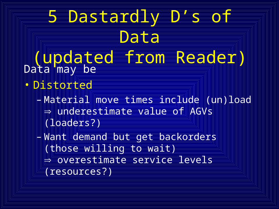
5 Dastardly D’s of Data(updated from Reader)

Data may be

• Distorted– Material move times include (un)load underestimate value of AGVs (loaders?)

– Want demand but get backorders (those willing to wait) overestimate service levels (resources?)

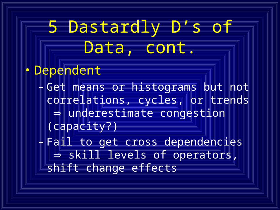
5 Dastardly D’s of Data, cont.

• Dependent– Get means or histograms but not correlations,

cycles, or trends underestimate congestion (capacity?)

– Fail to get cross dependencies skill levels of operators, shift change effects

5 Dastardly D’s of Data, cont.• Deleted

Data is censored (accounting) model not valid with new data

• DamagedData entry errors, collection errors (observer effect)

• Datedlast month’s data, different product mix valid models later fail validation

6th and 7th Dastardly D of Data...

• Doctored – well intentioned people tried to clean it up...

• Deceptive - any of the other problems might be intentional!

Data often used for performance evaluations,

or thought to be...

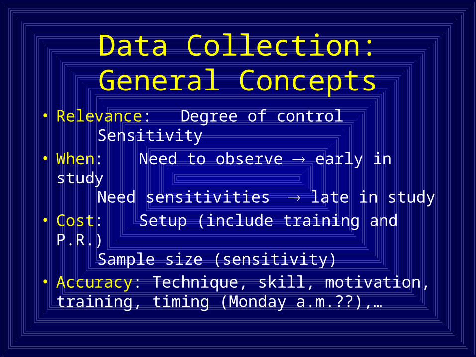
Data Collection: General Concepts

• Relevance: Degree of controlSensitivity

• When: Need to observe early in studyNeed sensitivities late in study

• Cost: Setup (include training and P.R.)Sample size (sensitivity)

• Accuracy: Technique, skill, motivation, training, timing (Monday a.m.??),…

Data Collection, cont.

• Precision: Technique, etc.Sample sizeSample interval (dependencies)

• Analysis: Error controlVerificationDependencies within data setDependencies between data sets

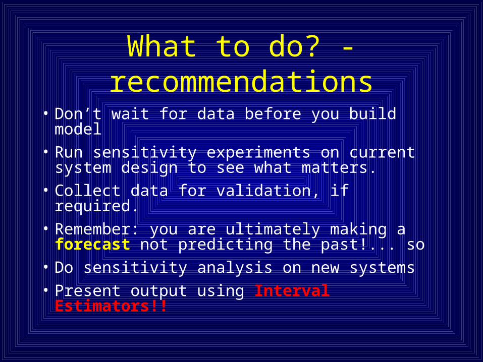
What to do? - recommendations

• Don’t wait for data before you build model

• Run sensitivity experiments on current system design to see what matters.

• Collect data for validation, if required.

• Remember: you are ultimately making a forecast not predicting the past!... so

• Do sensitivity analysis on new systems

• Present output using Interval Estimators!!

Simulation study

Formulate questions

Characterize answers

Design experiments

Develop, verify, refine model - as necessary

(Re)plan study and (re)secure resources

Do sensitivity analysis

If necessary, collect data

Analyze, Advise - and Caution

Start

Redesign and Run Experiments

Identify Prejudices

Enough time and money?

Anticipate system and human behavior

Code, re-code until have ‘no known errors’

Adjust Expectations