Non-parametric Approaches to Inference · Non-parametric Approaches to Inference Dr. Martyn...
51
Non-parametric Approaches to Inference Dr. Martyn McFarquhar Division of Neuroscience & Experimental Psychology The University of Manchester Edinburgh SPM course, 2017 1
Transcript of Non-parametric Approaches to Inference · Non-parametric Approaches to Inference Dr. Martyn...

Non-parametric Approaches to Inference
Dr. Martyn McFarquhar
Division of Neuroscience & Experimental Psychology The University of Manchester
Edinburgh SPM course, 20171

The parametric approachThe SPM approach is based on traditional parametric statistics
We makes assumptions about the form and parameters of the population distribution of the data
Non-parametric methods make no such assumptions
y ⇠ N (µ,�2)
y ⇠ Pois(�)
Important to understand the parametric approach in order to understand how non-parametric methods differ
2

The parametric approach
In the classical statistical framework the parameters of the population distribution are constants that we wish to estimate
μσ2
y1 y2 y3 yn…
3

The parametric approach
μσ2
y1 y2 y3 yn…
μσ2
y1 y2 y3 yn…
µ̂(1) µ̂(2) µ̂(3) µ̂(k)
μσ2
y1 y2 y3 yn…
Sample 2 …Sample 3Sample 1 Sample k
…Histogram of sampleMean
sampleMean
Frequency
-0.6 -0.4 -0.2 0.0 0.2 0.4 0.6
050
100
150
200
Sampling distribution of µ̂
μσ2
y1 y2 y3 yn…
4

The parametric approachThe sampling distribution is the probability distribution of a statistic estimated from a sample of size n
µ̂ ⇠ N✓µ,
�2
n
◆
As the sample mean is unbiased its average value is the true population value
It can tell us the most probable values of and how variable those values are
µ̂
If we assume that the population distribution is normal then the sampling distribution of is easily derivedµ̂
5

The parametric approach
Histogram of sample
sample
Frequency
-1.5 -1.0 -0.5 0.0 0.5 1.0 1.5
050
100
150
Histogram of sample
sample
Frequency
-1.5 -1.0 -0.5 0.0 0.5 1.0 1.5
050
100
150
200
250
Histogram of sample
sample
Frequency
-1.5 -1.0 -0.5 0.0 0.5 1.0 1.5
050
100
150
Histogram of sample
sample
Frequency
-1.5 -1.0 -0.5 0.0 0.5 1.0 1.5
050
100
150
n = 5, k = 1000 n = 10, k = 1000 n = 20, k = 1000 n = 100, k = 1000
µ̂ ⇠ N✓µ,
�2
n
◆
Although our interest in the true value of μ, all we know from the sampling distribution is that
• On average the sample mean will equal the true value • Larger samples lead to lower variance/higher precision of
the estimate
6

The parametric approachIn order to make a decision about the true value of μ we perform a hypothesis test
z =µ̂� µpVar(µ̂)
=µ̂p�2/n
t =µ̂� µqdVar(µ̂)
=µ̂p�̂2/n
This involves comparing our estimate of μ to some proposed value for the true μ — usually taken as 0
The difference is not very meaningful on its own as it depends on how variable the estimate is
If we divide the difference by its variability, we can produce a standardised index of how “meaningful” the difference is
7

The parametric approachWe are still left with a problem — how big does z or t need to be for us to make a decision about the proposed value of μ?
If we know the sampling distribution of the estimate of μ (and the estimate of 𝜎2) we can derive the distribution of z and t when the true value of μ equals the proposed value
This is the null distribution of the test statistic
From this we can calculate the p-value • Probability of finding a test statistic as large, or larger, if the
null were true
z ⇠ N (0, 1)
t ⇠ T (n� 1)
8

The parametric approachThe point is that
Assumed distribution for the population
Sampling distribution for the estimates
Null distribution of the test statistic
p-value
As such, if we use the p-value for inference we have to accept that its validity rests entirely on the assumed distribution of the population
9

The parametric approach
Assumed distribution for the population
Sampling distribution for the estimates
Null distribution of the test statistic
p-value
As such, if we use the p-value for inference we have to accept that its validity rests entirely on the assumed distribution of the population
If the population distribution is far from normal then • The sampling distribution of the estimates will be wrong • The null distribution of the test statistic will be wrong • The p-value will be wrong
The point is that
10

Non-parametric approachesThe validity of parametric approaches rest on assumptions about the distribution in the population
Non-parametric approaches do not make any assumptions about the population distribution — their validity does not rely on assuming a probability model for the population
Range of non-parametric procedures that you may be aware of • Friedman’s ANOVA • Kruskall-Wallis Test • Mann-Whitney U • Wilcoxon signed rank test
As computing power has increased the use of such tests has been somewhat overshadowed by resampling methods
11

The resampling solutionThere are a number of different resampling methods
• Bootstrap• Jackknife• Permutation testing
In neuroimaging the dominant approach is becoming permutation tests — the most straightforward way of arriving at non-parametric versions of the p-value
No matter the approach, the principle is the same • We treat our sample as a proxy for the population • Use a specific scheme to (re)sample values from our sample • Do this many times recomputing values of interest to build up
a distribution that can be used for inference
12

The permutation test
Use our data to approximate the null and thus calculate p-values without assuming any form for the population distribution
Permutation testing was originally developed by Fisher & Pitman during the 1930s
The use of parametric methods came about because it was impractical to perform permutation tests without computers
13

The permutation test
The use of parametric methods came about because it was impractical to perform permutation tests without computers
“If Fisher…had access to modern computers, it is likely that permutation
tests would be the standard procedure”
- Salkind (2010) Encyclopedia of Research Design
Permutation testing was originally developed by Fisher & Pitman during the 1930s
Use our data to approximate the null and thus calculate p-values without assuming any form for the population distribution
14

The permutation testExample of two groups
The key concept in permutation testing is rearranging the data labels
3 A
6 A
9 A
7 B
4 B1 B
Mean of A = 6 Mean of B = 4
3 B
6 A
9 B
7 A
4 B1 A
Mean of A = 4.66 Mean of B = 5.33
Difference = 2 Difference = 0.67
Original data Permuted data
15

The permutation testExample of two groups
For two groups of three subjects there are 20 different orderings of the group labels
1. AAABBB 2. AABABB3. AABBAB4. AABBBA5. ABAABB6. ABABAB7. ABABBA8. ABBAAB9. ABBABA10. ABBBAA
11. BAAABB12. BAABAB13. BAABBA14. BABAAB15. BABABA16. BABBAA17. BBAAAB18. BBAABA19. BBABAA20. BBBAAA
For each rearrangement we calculate the statistic of interest and save it
✓6
3
◆=
6!
3!(6� 3)!= 20
16

The permutation testExample of two groups
For two groups of three subjects there are 20 different orderings of the group labels
1. AAABBB 2. AABABB3. AABBAB4. AABBBA5. ABAABB6. ABABAB7. ABABBA8. ABBAAB9. ABBABA10. ABBBAA
11. BAAABB12. BAABAB13. BAABBA14. BABAAB15. BABABA16. BABBAA17. BBAAAB18. BBAABA19. BBABAA20. BBBAAA
✓6
3
◆=
6!
3!(6� 3)!= 20
Importantly the original order is included
For each rearrangement we calculate the statistic of interest and save it
17

The permutation testExample of two groups
By rearranging the labels we are calculating the test statistic under the null hypothesis of no difference
By saving each value we build an approximate null distribution
Once we have this distribution we can calculate the probability of getting our original test statistic, or larger, under the null
This gives us an approximate p-value
Histogram of meanDiff
meanDiff
Frequency
-1.5 -1.0 -0.5 0.0 0.5 1.0 1.5
0200
400
600
800
18

The permutation testRearranging the data
Generally speaking it is not the labels that we rearrange, rather it is the data itself
For simple models of groups this is the same as rearranging the labels
3 A
6 A
9 A7 B
4 B
1 B
6 A
7 A
1 A3 B
9 B
4 B
Mean of A = 6 Mean of B = 4
Mean of A = 4.66 Mean of B = 5.33
Original data Permuted data
19

The permutation testRearranging the data
For simple models of groups this is the same as rearranging the labels
18 10
26 10
34 1017 11
28 11
14 12
17 10
34 10
26 1018 11
14 11
28 12
Original data Permuted data
Slope = -5.5 Slope = -1
More general — allows us to permute models with no labels
Generally speaking it is not the labels that we rearrange, rather it is the data itself
20

The permutation testConceptual justification for permutations
The null hypothesis under rearrangement is that there is no relationship between the outcome variable and the predictor variables
As such, we can see what values we would get if those pairings were arbitrary
As such, the pairing of outcome values and predictor values is arbitrary
By breaking that pairing through rearrangement we create a realisation of the claim under the null
Our ability to do this relies on assumptions of exchangeability
21

The permutation testExchangeability
Formally, exchangeability means that under the null the joint distribution of the data do not change under rearrangement
Y = X� + ✏
✏ ⇠ N (0,�2I)
Any ordering of Y will lead to errors that are distributed as above
Designs that this precludes: • Groups with difference variances • Repeated measures/non-independent data
These can be incorporated using assumptions of weak exchangeability
22

The permutation testExchangeability — equal variance
Original error distributions for group A and B
Error distribution for row swapping 1
Error distribution for row swapping 2
Under rearrangement the errors are conceivably drawn from the same distribution as the original groups
-4 -2 0 2 4
0.0
0.2
0.4
0.6
-4 -2 0 2 4
0.0
0.2
0.4
0.6
-4 -2 0 2 40.00.20.40.60.8
-4 -2 0 2 4
0.00.20.40.60.8
-4 -2 0 2 4
0.0
0.4
0.8
-4 -2 0 2 4
0.0
0.2
0.4
0.6
-4 -2 0 2 4
0.0
0.2
0.4
0.6
-4 -2 0 2 40.0
0.4
0.8
23
-20 -10 0 10 20
0.0
0.2
0.4
-20 -10 0 10 20
0.00
0.03
0.06
-20 -10 0 10 200.00
0.10
-20 -10 0 10 20
0.00
0.10
0.20
-20 -10 0 10 20
0.00
0.10
-20 -10 0 10 20
0.00
0.10
0.20
-20 -10 0 10 20
0.00
0.10
0.20
-20 -10 0 10 200.00
0.10
0.20
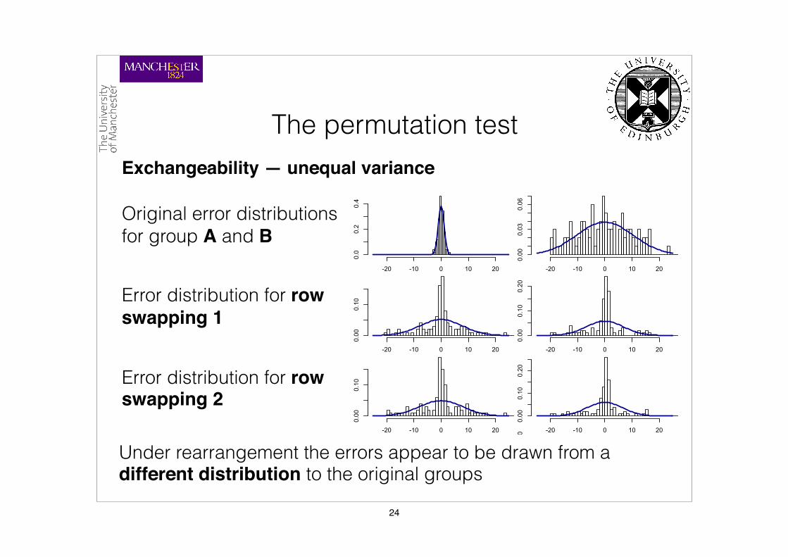
The permutation testExchangeability — unequal variance
Original error distributions for group A and B
Error distribution for row swapping 1
Error distribution for row swapping 2
Under rearrangement the errors appear to be drawn from a different distribution to the original groups
24
The permutation testExchangeability
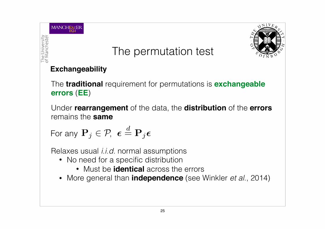
The traditional requirement for permutations is exchangeable errors (EE)
Under rearrangement of the data, the distribution of the errors remains the same
For any , ✏ d= Pj✏Pj 2 P
Relaxes usual i.i.d. normal assumptions • No need for a specific distribution
• Must be identical across the errors • More general than independence (see Winkler et al., 2014)
25

For any , ✏ d= Sj✏Sj 2 S
The permutation testExchangeability
A less restrictive assumption is independent and symmetric errors (ISE) — allows for errors that are not exchangeable
If both EE and ISE we can row-swap and sign-flip
Under sign-flipping of the data, the distribution of the errors remains the same
Relaxes usual i.i.d. normal assumptions • No need for a specific distribution
• Must be identical and symmetric • Independence is a necessity
26

The permutation testWeak exchangeability
Sometimes neither EE nor ISE can be assumed for the data as a whole — with a blocked structure then EE or ISE can be assumed at the level of the blocks
Example: Difference variances)IS
E
}}
EEEE
Note that row-swapping within each group will have no effect on the group means
Within block exchangeability
27

The permutation testWeak exchangeability
Sometimes neither EE nor ISE can be assumed for the data as a whole — with a blocked structure then EE or ISE can be assumed at the level of the blocks
Example: Repeated measures
)IS
E}}
}
}
Sub 1
Sub 2
Sub 3
Sub 4
EE
)Cannot swap rows or perform sign flips within a subject
Can swap rows and sign flip subjects as a whole
Between block exchangeability
28

The permutation testSign flipping for different variance groups
Original error distributions for group A and B
Error distribution for sign-flipping 1
Error distribution for sign-flipping 2
By using sign-flipping alone we can now conceive of the errors as drawn from the same distributions as the original data
-20 -10 0 10 20
0.0
0.2
0.4
-20 -10 0 10 20
0.00
0.02
0.04
0.06
-20 -10 0 10 20
0.0
0.2
0.4
0.6
-20 -10 0 10 20
0.00
0.03
0.06
-20 -10 0 10 20
0.0
0.2
0.4
-20 -10 0 10 20
0.00
0.03
0.06
-20 -10 0 10 20
0.0
0.2
0.4
-20 -10 0 10 20
0.00
0.02
0.04
0.06
29

The permutation testSign flipping for different variance groups
Y1 <- rnorm(100, 10, 1)Y2 <- rnorm(100, 10, 5)
Y <- c(Y1,Y2)Groups <- as.factor(c(rep("A",100), rep("B",100)))
paraTval <- t.test(Y ~ Groups)$stat
tdist <- rep(0,10000)
for (i in 1:10000){ signFlips <- sample(c(-1,1), size=200, replace=TRUE)newY <- signFlips*Ytdist[i] <- t.test(newY ~ Groups)$stat
}
permPval <- mean(abs(tdist) >= paraTval)
R Code
> permPval[1] 0.3407
> t.test(Y ~ Groups)
Welch Two Sample t-test
data: Y by Groupst = 0.94409, df = 107.24, p-value = 0.3472
Random sign-flipping is enough to break the connection between the outcome and predictors without rearrangement
30

Permutation testing in the GLMPermutation matrix
We can rearrange and/or sign-flip the data by pre-multiplying with a permutation matrix
exchangeability blocks, and the choice of an appropriate statistic forthese cases.
p-ValuesRegardless of the choice of the test statistic, p-values offer a common
measure of evidence against the null hypothesis. For a certain test statis-tic T, which can be any of those discussed above, and a particular ob-served value T0 of this statistic after the experiment has beenconducted, the p-value is the probability of observing, by chance, atest statistic equal or larger than the one computed with the observedvalues, i.e., P(T ≥ T0|H0). Although here we only consider one-sidedtests, where evidence against H0 corresponds to larger values of T0,two-sided or negative-valued tests and their p-values can be similarlydefined. In parametric settings, under a number of assumptions, the p-values can be obtained by referring to the theoretical distribution ofthe chosen statistic (such as the F distribution), either through aknown formula, or using tabulated values. In non-parametric settings,these assumptions are avoided. Instead, the data are randomly shuffled,many times, in amanner consistentwith the null hypothesis. Themodelis fitted repeatedly once for every shuffle, and for each fit a new realisa-tion of the statistic, Tj⁎, is computed, being j a permutation index. An em-pirical distribution of T⁎ under the null hypothesis is constructed, and
from this null distribution a p-value is computed as 1J∑ j I T⁎
j ≥T0
! ",
where J is the number of shufflings performed, and I(∙) is the indicatorfunction. From this it can be seen that the non-parametric p-valuesare discrete, with each possible p-value being a multiple of 1/J. It is im-portant to note that the permutation distribution should include the ob-served statistic without permutation (Edgington, 1969; Phipson andSmyth, 2010), and thus the smallest possible p-value is 1/J, not zero.
Permutations and exchangeability
Perhaps the most important aspect of permutation tests is the man-ner in which data are shuffled under the null hypothesis. It is the nullhypothesis, together with assumptions about exchangeability, whichdetermines the permutation strategy. Let the j-th permutation beexpressed by Pj, a N × N permutation matrix, a matrix that has all ele-ments being either 0 or 1, each row and column having exactly one 1(Fig. 1a). Pre-multiplication of a matrix by Pj permutes its rows. We de-note P ¼ P j
# $the set of all permutation matrices under consideration,
indexed by the subscript j. We similarly define a sign flipping matrix Sj,a N × N diagonal matrix whose non-zero elements consist only of +1or −1 (Fig. 1b). Pre-multiplication of a matrix by Sj implements a setof sign flips for each row. Likewise, S ¼ S j
# $denotes the set of all sign
flipping matrices under consideration. We consider also both schemestogether, whereB j ¼ P j′S j″ implements sign flips followed by permuta-tion; the set of all possible such transformations is denoted as B = {Bj}.Throughout the paper, we use generic terms as shuffling or rearrange-ment whenever the distinction between permutation, sign flippingor combined permutation with sign flipping is not pertinent. Finally,let β̂
"j and Tj⁎, respectively, be the estimated regression coefficients
and the computed statistic for the shuffling j.The essential assumption of permutationmethods is that, for a given
set of variables, their joint probability distribution does not change if theyare rearranged. This can be expressed in terms of exchangeable errors orindependent and symmetric errors, each of these weakening differentassumptions when compared to parametric methods.
Exchangeable errors (EE) is the traditional permutation requirement(Good, 2005). The formal statement is that, for any permutation P j∈P,ϵdP jϵ, where the symbol d denotes equality of distributions. In otherwords, the errors are considered exchangeable if their joint distributionis invariant with respect to permutation. Exchangeability is similar to,yet more general than, independence, as exchangeable errors can haveall-equal and homogeneous dependence. Relative to the common
parametric assumptions of independent, normally and identically dis-tributed (iid) errors, EE relaxes two aspects. First, normality is no longerassumed, although identical distributions are required. Second, theindependence assumption isweakened slightly to allow exchangeabilitywhen the observations are not independent, but their joint distributionismaintained after permutation.While exchangeability is a general con-dition that applies to any distribution, we note that the multivariatenormal distribution is indeed exchangeable if all off-diagonal elementsof the covariance matrix are identical to each other (not necessarilyequal to zero) and all the diagonal elements are also identical to eachother. In parametric settings, such dependence structure is often re-ferred to as compound symmetry.
Independent and symmetric errors (ISE) can be considered formeasurements that arise, for instance, from differences between twogroups if the variances are not assumed to be the same. The formalstatement for permutation under ISE is that for any sign flipping matrixS j∈S; ϵd S jϵ, that is, the joint distribution of the error terms is invariantwith respect to sign flipping. Relative to the parametric assumptions ofindependent, normally and identically distributed errors, ISE relaxesnormality, although symmetry (i.e., non-skewness) of distributions is
−4.01
−2.97
−1.98
0.00
+0.96
−1.01
+3.00
+4.02
+2.03
Permutationmatrix
Originaldata
Permuteddata
0 0 0 0 00 0 0 00 0 0
0 0 0 00 0 0
0 0 0
000
00
0 00 0
0 0 0
1
0 00
0 0 00
0 00 0 0
0 00 00 0
0 00 0
0 0 0
000
0
00
00
00
0
00
11
11
11
11
−4.01−2.97−1.98
0.00+0.96
−1.01
+3.00+4.02
+2.03
(a)
+4.01+2.97−1.98
0.00+0.96
−1.01
+3.00−4.02
−2.03
−4.01−2.97−1.98
0.00+0.96
−1.01
+3.00+4.02
+2.03
Sign-flippingmatrix
Originaldata
Sign-flippeddata
0 0 0 00 0 0 00 0 0
0 0 0 00 0 0
0 0 0
000
00
00
0 00 0
00 0 0
00 0
0 00 00 0
0 00 0
0 0 0
00
0
00
00
00
00
00
00
0
0
00
−1−1
+1+1
−1+1
0
−1
−1+1
(b)
+4.01
+2.97
−1.98
0.00
+0.96
−1.01
+3.00
−4.02
−2.03
× =
× =
× =
Permutation andsign-flipping matrix
Originaldata
Permuted &sign-flipped
0 0 0 0 00 0 0 00 0 0
0 0 0 00 0 0
0 0 0
000
00
0 00 0
0 0 0
+1
0 00
0 0 00
0 00 0 0
0 00 00 0
0 00 0
0 0 0
000
0
00
00
00
0
00
−1−1
−1−1
+1+1
−1+1
−4.01−2.97−1.98
0.00+0.96
−1.01
+3.00+4.02
+2.03
(c)
Fig. 1. Examples of a permutation matrix (a), of a sign flippingmatrix (b), and of a matrixthat does permutation and sign flipping (c). Pre-multiplication by a permutation matrixshuffles the order of the data, whereas by a sign flipping matrix changes the sign of arandom subset of data points.
383A.M. Winkler et al. / NeuroImage 92 (2014) 381–397
Winkler et al. (2014) NeuroImage
The original data can be seen as pre-multiplication with an identity permutation matrix
31

Permutation testing in the GLMPermutation matrix
exchangeability blocks, and the choice of an appropriate statistic forthese cases.
p-ValuesRegardless of the choice of the test statistic, p-values offer a common
measure of evidence against the null hypothesis. For a certain test statis-tic T, which can be any of those discussed above, and a particular ob-served value T0 of this statistic after the experiment has beenconducted, the p-value is the probability of observing, by chance, atest statistic equal or larger than the one computed with the observedvalues, i.e., P(T ≥ T0|H0). Although here we only consider one-sidedtests, where evidence against H0 corresponds to larger values of T0,two-sided or negative-valued tests and their p-values can be similarlydefined. In parametric settings, under a number of assumptions, the p-values can be obtained by referring to the theoretical distribution ofthe chosen statistic (such as the F distribution), either through aknown formula, or using tabulated values. In non-parametric settings,these assumptions are avoided. Instead, the data are randomly shuffled,many times, in amanner consistentwith the null hypothesis. Themodelis fitted repeatedly once for every shuffle, and for each fit a new realisa-tion of the statistic, Tj⁎, is computed, being j a permutation index. An em-pirical distribution of T⁎ under the null hypothesis is constructed, and
from this null distribution a p-value is computed as 1J∑ j I T⁎
j ≥T0
! ",
where J is the number of shufflings performed, and I(∙) is the indicatorfunction. From this it can be seen that the non-parametric p-valuesare discrete, with each possible p-value being a multiple of 1/J. It is im-portant to note that the permutation distribution should include the ob-served statistic without permutation (Edgington, 1969; Phipson andSmyth, 2010), and thus the smallest possible p-value is 1/J, not zero.
Permutations and exchangeability
Perhaps the most important aspect of permutation tests is the man-ner in which data are shuffled under the null hypothesis. It is the nullhypothesis, together with assumptions about exchangeability, whichdetermines the permutation strategy. Let the j-th permutation beexpressed by Pj, a N × N permutation matrix, a matrix that has all ele-ments being either 0 or 1, each row and column having exactly one 1(Fig. 1a). Pre-multiplication of a matrix by Pj permutes its rows. We de-note P ¼ P j
# $the set of all permutation matrices under consideration,
indexed by the subscript j. We similarly define a sign flipping matrix Sj,a N × N diagonal matrix whose non-zero elements consist only of +1or −1 (Fig. 1b). Pre-multiplication of a matrix by Sj implements a setof sign flips for each row. Likewise, S ¼ S j
# $denotes the set of all sign
flipping matrices under consideration. We consider also both schemestogether, whereB j ¼ P j′S j″ implements sign flips followed by permuta-tion; the set of all possible such transformations is denoted as B = {Bj}.Throughout the paper, we use generic terms as shuffling or rearrange-ment whenever the distinction between permutation, sign flippingor combined permutation with sign flipping is not pertinent. Finally,let β̂
"j and Tj⁎, respectively, be the estimated regression coefficients
and the computed statistic for the shuffling j.The essential assumption of permutationmethods is that, for a given
set of variables, their joint probability distribution does not change if theyare rearranged. This can be expressed in terms of exchangeable errors orindependent and symmetric errors, each of these weakening differentassumptions when compared to parametric methods.
Exchangeable errors (EE) is the traditional permutation requirement(Good, 2005). The formal statement is that, for any permutation P j∈P,ϵdP jϵ, where the symbol d denotes equality of distributions. In otherwords, the errors are considered exchangeable if their joint distributionis invariant with respect to permutation. Exchangeability is similar to,yet more general than, independence, as exchangeable errors can haveall-equal and homogeneous dependence. Relative to the common
parametric assumptions of independent, normally and identically dis-tributed (iid) errors, EE relaxes two aspects. First, normality is no longerassumed, although identical distributions are required. Second, theindependence assumption isweakened slightly to allow exchangeabilitywhen the observations are not independent, but their joint distributionismaintained after permutation.While exchangeability is a general con-dition that applies to any distribution, we note that the multivariatenormal distribution is indeed exchangeable if all off-diagonal elementsof the covariance matrix are identical to each other (not necessarilyequal to zero) and all the diagonal elements are also identical to eachother. In parametric settings, such dependence structure is often re-ferred to as compound symmetry.
Independent and symmetric errors (ISE) can be considered formeasurements that arise, for instance, from differences between twogroups if the variances are not assumed to be the same. The formalstatement for permutation under ISE is that for any sign flipping matrixS j∈S; ϵd S jϵ, that is, the joint distribution of the error terms is invariantwith respect to sign flipping. Relative to the parametric assumptions ofindependent, normally and identically distributed errors, ISE relaxesnormality, although symmetry (i.e., non-skewness) of distributions is
−4.01
−2.97
−1.98
0.00
+0.96
−1.01
+3.00
+4.02
+2.03
Permutationmatrix
Originaldata
Permuteddata
0 0 0 0 00 0 0 00 0 0
0 0 0 00 0 0
0 0 0
000
00
0 00 0
0 0 0
1
0 00
0 0 00
0 00 0 0
0 00 00 0
0 00 0
0 0 0
000
0
00
00
00
0
00
11
11
11
11
−4.01−2.97−1.98
0.00+0.96
−1.01
+3.00+4.02
+2.03
(a)
+4.01+2.97−1.98
0.00+0.96
−1.01
+3.00−4.02
−2.03
−4.01−2.97−1.98
0.00+0.96
−1.01
+3.00+4.02
+2.03
Sign-flippingmatrix
Originaldata
Sign-flippeddata
0 0 0 00 0 0 00 0 0
0 0 0 00 0 0
0 0 0
000
00
00
0 00 0
00 0 0
00 0
0 00 00 0
0 00 0
0 0 0
00
0
00
00
00
00
00
00
0
0
00
−1−1
+1+1
−1+1
0
−1
−1+1
(b)
+4.01
+2.97
−1.98
0.00
+0.96
−1.01
+3.00
−4.02
−2.03
× =
× =
× =
Permutation andsign-flipping matrix
Originaldata
Permuted &sign-flipped
0 0 0 0 00 0 0 00 0 0
0 0 0 00 0 0
0 0 0
000
00
0 00 0
0 0 0
+1
0 00
0 0 00
0 00 0 0
0 00 00 0
0 00 0
0 0 0
000
0
00
00
00
0
00
−1−1
−1−1
+1+1
−1+1
−4.01−2.97−1.98
0.00+0.96
−1.01
+3.00+4.02
+2.03
(c)
Fig. 1. Examples of a permutation matrix (a), of a sign flippingmatrix (b), and of a matrixthat does permutation and sign flipping (c). Pre-multiplication by a permutation matrixshuffles the order of the data, whereas by a sign flipping matrix changes the sign of arandom subset of data points.
383A.M. Winkler et al. / NeuroImage 92 (2014) 381–397
We can rearrange and/or sign-flip the data by pre-multiplying with a permutation matrix
Winkler et al. (2014) NeuroImage32

Permutation testing in the GLMPermutation matrix
Within-block exchangeability
Ridgway, 2009), they often only approached particular cases, did notconsider the possibility of permutation of blocks of observations, didnot use full matrix notation as more common in neuroimaging litera-ture, and often did not consider implementation complexities due tothe large size of imaging datasets. In this section we focus on the Freed-man–Lane and the Smith methods, which, as we show in Permutationstrategies, produce the best results in terms of control over error ratesand power.
The Freedman–Lane procedure (Freedman and Lane, 1983) can beperformed through the following steps:
1. Regress Y against the full model that contains both the effects ofinterest and the nuisance variables, i.e. Y = Xβ + Zγ + ϵ. Use theestimated parameters β̂ to compute the statistic of interest, and callthis statistic T0.
2. RegressY against a reducedmodel that contains only the nuisance ef-fects, i.e. Y= Zγ+ ϵZ, obtaining estimated parameters γ̂ and estimat-ed residuals ϵ̂Z.
3. Compute a set of permuted data Yj∗. This is done by pre-multiplying
the residuals from the reduced model produced in the previousstep, ϵ̂Z, by a permutation matrix, Pj, then adding back the estimatednuisance effects, i.e. Y!
j ¼ P jϵ̂Z þ Zγ̂.4. Regress the permuted data Yj
∗ against the full model, i.e. Yj∗ = Xβ +
Zγ+ ϵ, and use the estimated β̂!j to compute the statistic of interest.
Call this statistic Tj∗.5. Repeat Steps 2–4many times to build the reference distribution of T⁎
under the null hypothesis.6. Count howmany times Tj∗ was found to be equal to or larger than T0,
and divide the count by the number of permutations; the result is thep-value.
For Steps 2 and 3, it is not necessary to actually fit the reducedmodelat each point in the image. The permuted dataset can equivalently beobtained as Yj
∗=(PjRZ+HZ)Y, which is particularly efficient for neuro-imaging applications in the typical case of a single design matrix for allimage points, as the term PjRZ + HZ is then constant throughout theimage and so, needs to be computed just once. Moreover, the additionof nuisance variables back in Step 3 is not strictly necessary, and themodel can be expressed simply as PjRZY= Xβ+ Zγ + ϵ, implying thatthe permutations can actually be performed just by permuting the rowsof the residual-forming matrix RZ. The Freedman–Lane strategy is theone used in the randomise algorithm, discussed in Appendix B.
The rationale for this permutationmethod is that, if the null hypoth-esis is true, then β = 0, and so the residuals from the reduced modelwith only nuisance variables, ϵZ, should not be different than the resid-uals from the full model, ϵ, and can, therefore, be used to create thereference distribution from which p-values can be obtained.
The Smith procedure consists of orthogonalising the regressors ofinterest with respect to the nuisance variables. This is done by pre-multiplication of X by the residual forming matrix due to Z, i.e., RZ,then permuting this orthogonalised version of the regressors of interest.The nuisance regressors remain in the model.2
For both the Freedman–Lane and the Smith procedures, if the er-rors are independent and symmetric (ISE), the permutation matricesPj can be replaced for sign flipping matrices Sj. If both EE and ISE areconsidered appropriate, then permutation and sign flipping can beused concomitantly.
Restricted exchangeabilitySomeexperimental designs involvemultiple observations from each
subject, or the subjectsmay come fromgroups thatmay possess charac-teristics that may render their distributions not perfectly comparable.Both situations violate exchangeability. However, when the depen-dence between observations has a block structure, this structure canbe taken into account when permuting the model, restricting the setof all otherwise possible permutations to only those that respect the re-lationship between observations (Pesarin, 2001); observations that areexchangeable only in some subsets of all possible permutations are saidweakly exchangeable (Good, 2002). The EE and ISE assumptions are thenasserted at the level of these exchangeability blocks, rather than for eachobservation individually. The experimental hypothesis and the studydesign determine how the EBs should be formed and how the permuta-tion or sign flipping matrices should be constructed. Except Huh–Jhun,the other methods in Table 2 can be applied at the block level as inthe unrestricted case.
Within-block exchangeability.Observations that share the same depen-dence structure, either assumed or known in advance, can be used todefine EBs such that EE are asserted with respect to these blocks only,and the empirical distribution is constructed by permuting exclu-sively within block, as shown in Fig. 2. Once the blocks have beendefined, the regression of nuisance variables and the construction ofthe reference distribution can follow strategies as Freedman–Laneor Smith, as above. The ISE, when applicable, is transparent to this kindof block structure, so that the sign flips occur as under unrestrictedexchangeability. For within-block exchangeability, in general each EB
corresponds to a VG for the computation of the test statistic. SeeAppendix C for examples.
Whole-block exchangeability. Certain experimental hypotheses mayrequire the comparison of sets of observations to be treated as awhole, being not exchangeable within set. Exchangeability blocks canbe constructed such that each include, in a consistent order, all theobservations pertaining to a given set and, differently than in within-block exchangeability, here each block is exchanged with the otherson their entirety, while maintaining the order of observations withinblock unaltered. For ISE, the signs are flipped for all observations withinblock at once. Variance groups are not constructed one per block;instead, each VG encompasses one or more observations per block, allin the same order, e.g., one VG with the first observation of each block,
2 We name this method after Smith because, although orthogonalisation is a wellknownprocedure, it does not seem to have been proposed by anyone to address the issueswith permutation methods with the GLM until Smith and others presented it in a confer-ence poster (Nichols et al., 2008). We also use the eponym to keep it consistent withRidgway (2009),and to keep the convention of calling the methods by the earliest authorthat we could identify as the proponent for eachmethod, even though thismethod seemsto have been proposed by an anonymous referee of O'Gorman (2005).
Permutationmatrix
Sign-flippingmatrix
0 0 00 0 0
0 0 00 0 0 00 0 00 0 0 0
000
0
0
00
00
0
0 0 0 00 0 00 0 0 0
00
0 00 0
0000
00
0 0 00 00 0 0
0
0 00 0
00
0000
+1+1
−1+1
+1−1
+1−1
+1
Block 1
Block 2
Block 3
0 00 0
0 00 0 00 0 00 0 0 0
000
0
00
0
0
0 0 00 0 00 0 0
0
0 00 0
0000
00
0 0 00 00 0 0
0
0 00 0
00
0000
11
11
11
11
1
000
00
00
00 0
Fig. 2. Left: Example of a permutation matrix that shuffles data within block only. Theblocks are not required to be of the same size. The elements outside the diagonal blocksare always equal to zero, such that data cannot be swapped across blocks. Right: Exampleof a sign flipping matrix. Differently than within-block permutation matrices, here signflipping matrices are transparent to the definitions of the blocks, such that the block def-initions do not need to be taken into account, albeit their corresponding variance groupsare considered when computing the statistic.
385A.M. Winkler et al. / NeuroImage 92 (2014) 381–397
another with the second of each block and so on. Consequently, allblocks must be of the same size, and all with their observations orderedconsistently, either for EE or for ISE. Examples of permutation and signflipping matrices for whole block permutation are shown in Fig. 3. SeeAppendix C for examples.
Variance groups mismatching exchangeability blocks. While variancegroups can be defined implicitly, as above, according to whetherwithin- or whole-block permutation is to be performed, this is notcompulsory. In some cases the EBs are defined based on the non-independence between observations, even if the variances across allobservations can still be assumed to be identical. See Appendix C foran example using a paired t-test.
Choice of the configuration of exchangeability blocks. The choice betweenwhole-block and within-block is based on assumptions, or on knowl-edge about the non-independence between the error terms, as well ason the need to effectively break, at each permutation, the relationshipbetween the data and the regressors of interest. Whole-block can beconsidered whenever the relationship within subsets of observations,all of the same size, is not identical, but follows a pattern that repeats it-self at each subset. Within-block exchangeability can be consideredwhen the relationship between all observations within a subset is iden-tical, even if the subsets are not of the same size, or the relationship itselfis not the same for all of them. Whole-block and within-block arestraightforward ways to determine the set of valid permutations, butare not the only possibility to determine them, nor are mutually exclu-sive. Whole-block and within-block can be mixed with each other invarious levels of increasing complexity.
Choice of the statistic with exchangeability blocks. All the permutationstrategies discussed in the previous section can be used with virtuallyany statistic, the choice resting on particular applications, and constitut-ing a separate topic. The presence of restrictions on exchangeability and
variance groups reduces the choices available, though. The statistics Fand t, described in Model and notation, are pivotal and follow knowndistributions when, among other assumptions, the error terms for allobservations are identically distributed. Under these assumptions, allthe errors terms can be pooled to compute the residual sum of squares(the term ϵ̂′ ϵ̂ in Eq. (3)) and so, the variance of the parameter estimates.This forms the basis for parametric inference, and is also useful for non-parametric tests. However, the presence of EBs can be incompatiblewith the equality of distributions across all observations, with the unde-sired consequence that pivotality is lost, as shown in the Results. Al-though these statistics can still be used with permutation methods ingeneral, the lack of pivotality for imaging applications can cause prob-lems for correction of multiple testing. When exchangeability blocksand associated variance groups are present, a suitable statistic can becomputed as:
G ¼ψ̂′C C′ M′WM
! "−1C
# $−1C′ψ̂
Λ " rank Cð Þð6Þ
whereW is aN× N diagonal weightingmatrix that has elementsWnn ¼
∑n′∈gnRn′n′
ϵ̂′gn ϵ̂gn, where gn represents the variance group to which the n-th ob-
servation belongs, Rn′n′ is the n′-th diagonal element of the residualforming matrix, and ϵ̂gn is the vector of residuals associated with thesame VG.3 In other words, each diagonal element of W is the reciprocalof the estimated variance for their corresponding group. This varianceestimator is equivalent to the one proposed by Horn et al. (1975). Theremaining term in Eq. (6) is given by (Welch, 1951):
Λ ¼ 1þ 2 s−1ð Þs sþ 2ð Þ
X
g
1Xn∈g
Rnn1−
Xn∈g
Wnn
trace Wð Þ
0
@
1
A2
ð7Þ
wheres ¼rank(C) as before. The statisticGprovides a generalisation of anumber of well known statistical tests, some of them summarised inTable 3. When there is only one VG, variance estimates can be pooledacross all observations, resulting in Λ = 1 and so, G = F. If W = V−1,the inverse of the true covariance matrix, G is the statistic for an F-testin a weighted least squares model (WLS) (Christensen, 2002). If thereare multiple variance groups, G is equivalent to the v2 statistic for theproblemof testing themeans for these groups under no homoscedastic-ity assumption, i.e., when the variances cannot be assumed to be allequal (Welch, 1951).4 If, despite heteroscedasticity, Λ is replaced by 1,G is equivalent to the James' statistic for the same problem (James,
1951). When rank(C) = 1, and if there are more than one VG, sign β̂! "
ffiffiffiffiG
pis the well-known v statistic for the Behrens–Fisher problem
(Aspin and Welch, 1949; Fisher, 1935b); with only one VG present, thesame expression produces the Student's t statistic, as shown earlier. Ifthe definition of the blocks and variance groups is respected, all theseparticular cases produce pivotal statistics, and the generalisation pro-vided by G allows straightforward implementation.
Number of permutations
For a study with N observations, the maximum number of possiblepermutations is N!, and the maximum number of possible sign flips is2N. However, in the presence of B exchangeability blocks that are
0
001
11 0
0
00 1
100
1=
00
0 1
0 0 00 00 0 0
00 0 00 00 0 0
0
0 00 0
0000
0
0 00 0
0
0000
0
0
00 1
100
10
00
11
1
00
0
0
000
0000
000
0 00 0 0
00 00
11
00
001
00
Permutationmatrix
Identitymatrix
Blockpermutation
matrix
0
0
00 1
100
1=
0
0
000
0−1
+1−1
0 0 00 00 0 0
00 0 00 00 0 0
0
0 00 0
0000
0
0 00 0
0
0000
00
00 0
0
00
0
00
0
0
0 00 0 0
00 00
0
0
000
0−1
−1−1
+1+1
+1−1
−1−1
0 00 0
0
0000
Sign-flippingmatrix
Identitymatrix
Blocksign-flipping
matrix
(a)
(b)
Fig. 3. (a) Example of a permutation matrix that shuffles whole blocks of data. Theblocks need to be of the same size. (b) Example of a sign flipping matrix that changesthe signs of the blocks as a whole. Both matrices can be constructed by the Kroneckerproduct (represented by the symbol ⊗) of a permutation or a sign flipping matrix (withsize determined by the number of blocks) and an identity matrix (with size determinedby the number of observations per block).
3 Note that, for clarity, G is defined in Eq. (6) as a function of M, ψ and C in theunpartitioned model. With the partitioning described in the Appendix A, each of thesevariables is replaced by their equivalents in the partitioned, full model, i.e., [X Z], [β′ γ′]′and [Is × s 0s × (r − s)]′ respectively.
4 If the errors are independent and normally distributed, yet not necessarily with equalvariances (i.e., Λ≠ 1), parametric p-values for G can be approximated by referring to theF-distribution with degrees of freedom v1 = s and v2 = 2(s − 1)/3/(Λ − 1).
386 A.M. Winkler et al. / NeuroImage 92 (2014) 381–397
Whole-block exchangeability
Winkler et al. (2014) NeuroImage33
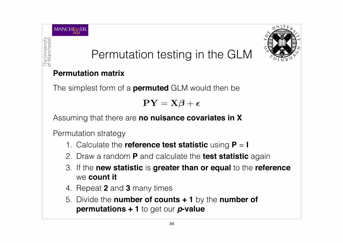
Permutation testing in the GLMPermutation matrix
The simplest form of a permuted GLM would then be
PY = X� + ✏
Assuming that there are no nuisance covariates in X
Permutation strategy 1. Calculate the reference test statistic using P = I 2. Draw a random P and calculate the test statistic again 3. If the new statistic is greater than or equal to the reference
we count it 4. Repeat 2 and 3 many times 5. Divide the number of counts + 1 by the number of
permutations + 1 to get our p-value34

Permutation testing in the GLM
% Generate some dataY(1:20) = normrnd(6,2,20,1);Y(21:40) = normrnd(5,2,20,1);
% Design matrix and contrastX = [ones(1,20) zeros(1,20); zeros(1,20) ones(1,20)]'; L = [1 -1];
% Reference modelbeta = inv(X'*X)*X'*Y;resid = Y - X*beta;sigma = (resid'*resid) / 38;refF = ((L*beta)' * inv(L*inv(X'*X)*L') * (L*beta)) / sigma;
% Parametric p-valueparaP = fcdf(refF, 1, 38, ‘upper');
Example in MATLAB
Randomly generate some data, fit a two-sample GLM with a contrast comparing the groups using an F-test
35

Permutation testing in the GLM
% Permutationscount = zeros(5000,1);for i = 1:5000 P = eye(40); P = P(randperm(40),:); Yperm = P*Y; betaPerm = inv(X'*X)*X'*Yperm; residPerm = Yperm - X*betaPerm; sigmaPerm = (residPerm'*residPerm) / 38; Fdist(i,1) = ((L*betaPerm)' * inv(L*inv(X'*X)*L') * (L*betaPerm)) / sigmaPerm; if Fdist(i,1) >= refF count(i) = 1; endend % Permutation p-valuepermP = (sum(count) + 1) / (5001);
Example in MATLAB
Across 5,000 repetitions create a random permutation matrix, pre-multiply the data, re-fit the model and recalculate the F-test
36

Permutation testing in the GLM
Strong correspondence between parametric and non-parametric p-values when data are normal
0 2 4 6 8 10 12 14 16 18 20Replication
0
0.2
0.4
0.6
0.8
1
p-value
ParametricPermutation
Example in MATLAB
37

Permutation testing in the GLMPermutation testing with nuisance covariates
So far we have only considered models with a single continuous covariate or single factor
In cases where we have multiple covariate/factors permutations become more difficult
Under the null of no effect for one covariate/factor there may still be other effects in the model that should be accounted for
If we just permuted the data, we will disrupt all the effects in the model — not looking at the model under the null of one effect being 0 with all other effects accounted for
38

Permutation testing in the GLMPermutation testing with nuisance covariates
The Freedman-Lane (Freedman & Lane, 1983) approach is
The permuted data Y* are given by
Y⇤ = X� + Z� + ✏
Y⇤ = P✏Z + Z� Residuals from the model containing only the nuisance effects
Can also express the model as
Effects of interest
(PRZ +HZ)Y = X� + Z� + ✏
Nuisance effects
39

Permutation testing in the GLMRandomise algorithm
The key steps in the randomise algorithm are:
1. The contrast is used to partition the model into effects of interest and nuisance effects
2. The model containing only nuisance effects is fit and nuisance partition residuals are formed
3. These residuals are permuted
4. The nuisance effects are added back, the full model is fit and the test statistic is calculated and saved
5. Steps 3 and 4 are repeated many times to build up the null distribution of the test statistic
40

Permutation tests in neuroimaging
Permutation methods can also provide a family wise error correction as an alternative to RFT
For each iteration we 1. Calculate the largest statistic in
the image 2. For each voxel compare the
reference statistic to the largest permuted statistic
The p-value is then the probability of finding a statistic as large, or larger, under the null anywhere in the image
Multiple comparisons correction
produce normalised greymatter images using the segmented tissue im-ages from the preprocessing.
One particular issue in using the MANOVA approach for modellingmultimodal data is that differentmodalities often provide images of dif-ferent resolution. For example, a typical structural MR image may havearound 10 times as many voxels as a typical task-based fMR image. Inorder for a voxel-by-voxel analysis to work, it is necessary to rescaleone of themodalities to match the other. Our own limited investigationof this issue suggests that results are relatively invariant towhether oneup-samples the functional to the dimensions of the structural, or down-samples the structural to the dimensions of the functional. Where thebenefit of resampling the higher resolution image becomes clear iswith the increase in computational speed and decrease in computation-al burden formodel estimation and inference by permutation, as well asa reduction in the number of hypothesis tests thatmust be corrected forat the voxel-level. That being said, the choice of approach will likely
depend on the modality of most interest, and the investigator's opinionon the trade-off between increased computational speed and the loss ofinformation engendered by interpolating a higher-resolution image tosmaller dimensions.
Another issue, typical to VBM investigations, is the necessity ofa correction for head size to allow for sensible between-subjectcomparisons. In SPM, it is possible to provide values to performproportional scaling of the images before the model is estimated.As there is no such facility in MRM, the proportional scaling was per-formed manually on the normalised grey matter images before theywere entered into the model. Specifically, the value at each voxel ofthe normalised grey matter images was divided by the participant'stotal intracranial volume (estimated using the Easy_volume toolhttp://www.sbirc.ed.ac.uk/cyril; as described in Pernet et al., 2009)to produce proportionally scaled versions of the DARTEL results.For the multivariate GLM, this strategy is preferable to entering thesevalues as covariates given that any covariate will influence all themodel parameters, irrespective of the modality. This could be seen asa disadvantage of the multivariate approach to multimodal integration,particularly in those cases where co-varying for a nuisance variablein one modality is seen as preferable to rescaling the raw data. Othercovariates that may be relevant for both modalities can be enteredinto the model directly, though for simplicity of presentation, we donot include any here. Only after the proportional scaling were thegrey matter images resampled to the same dimensions as the imagesof parameter estimates from the functional models. In addition, itis worth mentioning that at present the permutation approach imple-mented in MRM does not account for non-stationarity when usingcluster-level inference. As approaches to permutation that accommo-date non-uniform smoothness of the images have been proposed byHayasaka et al. (2004), this could be implemented in the future toallow researchers to appropriately use cluster-level statistics for analy-ses of data such as structural MR images.
As a final step, we produced a mask to restrict the analysis to onlyregions of grey matter. This was done by averaging the scaled andresampled grey matter images and then producing a binary imageincluding voxels with an intensity N0.2. Such an approach is in keepingwith the recommendations given by Ashburner (2010).
7.2. Model estimation and results
The group-level model used for these data consisted only of thegrouping variable for controls or rMDD. Themodel was therefore equiv-alent to amultivariate formof a simple two-sample t-test. As this designwas specified as a MANOVA model, the structural and functional datawere treated as non-commensurate. As such, the Cmatrix of the generallinear hypothesis test of the main effect of diagnosis was specified as I2.Results of this contrast, thresholded at an uncorrected p b 0.001, re-vealed a cluster of 48 voxels in the left lingual gyrus (peak at −15−73 −7 with F(2,25) = 19.26). Following up this result using dLDA atthe peak voxel revealed a single discriminant function with absolutevalues of the standardised weights given as 0.826 for the structural mo-dality and 0.850 for the functional modality. This result is particularlyinteresting because it suggests that, at this peak voxel, a near equal bal-ance of themodalities providesmaximal separation of the groups. Usingthe partial F-testmethodology described in Appendix B gives significantresults for both the structural and functional modalities (bothp b 0.001), suggesting that each modality is contributing to groupseparation.
Of further interest here is that conducting the univariate equivalentsof this analysis on each modality separately revealed smaller test statis-tics at this peak, as shown in Fig. 11. Here, a clear advantage of the mul-tivariate approach is seen as the individual results from the univariateanalyses have been strengthened by virtue of the fact that equivalentresults are seen across modalities. The results of the dLDA at this voxelenhance this interpretation given that nearly equal weight is given for
Fig. 9. Comparisons between the SPMGaussian random field,MRMpermutation, and SwEnon-parametric bootstrap approaches to FWE correction. The numbers above the imagesindicate the number of voxels surviving thresholding in each image. The permutation andbootstrap distributions are displayed with the 5% thresholds indicated. The originalmaximum reference test statistic has been cropped to make the histograms morereadable. For comparison, the 5% F threshold given by SPM12 was 28.40. Total time tocomplete the non-parametric approaches (in minutes) were MRM = 12.62, SwE =213.88.
Table 2P-value comparisons between the different FWE methods for the seven smallest maximareported by SPM.
Peak location (mm) p-GRF p-PERM p-BOOT
x y z
−45 −37 17 0.002 b 0.001 0.00142 −16 35 0.008 0.003 0.0040 −25 −1 0.019 0.006 0.00721 59 5 0.026 0.008 0.011−33 −1 −37 0.035 0.010 0.015−21 35 38 0.035 0.010 0.01551 11 2 0.047 0.011 0.020
p-GRF = FWE-corrected p-values from the SPM GRF approach.p-PERM=FWE-corrected p-values from theMRMpermutation approach (5000 reshuffles).p-BOOT = FWE-corrected p-values from the SwE non-parametric bootstrap approach(5000 bootstrap resamples).
384 M. McFarquhar et al. / NeuroImage 132 (2016) 373–389
Build the null distribution of largest test statistics
41

Permutation tests in neuroimaging
Though this is naturally suited to voxel inference we can extend the approach to cluster inference as well
Multiple comparisons correction
For each iteration we 1. Form clusters by thresholding the image using parametric p-values
2. Find the largest cluster in the image 3. Compare the size of each reference cluster to the largest
permuted cluster
Build the null distribution of largest clusters
The p-value is then the probability of finding a cluster as large, or larger, under the null anywhere in the image
42
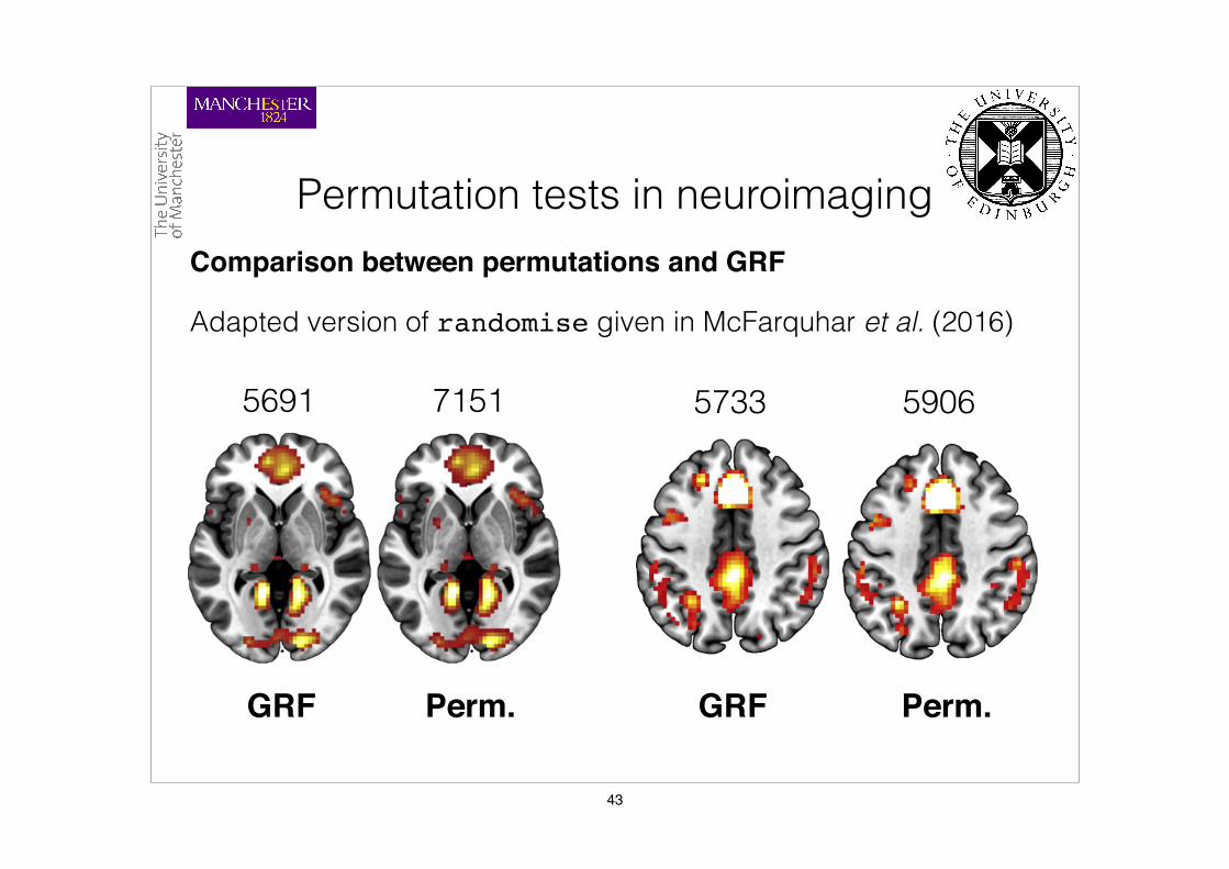
Comparison between permutations and GRF
Adapted version of randomise given in McFarquhar et al. (2016)
Permutation tests in neuroimaging
produce normalised greymatter images using the segmented tissue im-ages from the preprocessing.
One particular issue in using the MANOVA approach for modellingmultimodal data is that differentmodalities often provide images of dif-ferent resolution. For example, a typical structural MR image may havearound 10 times as many voxels as a typical task-based fMR image. Inorder for a voxel-by-voxel analysis to work, it is necessary to rescaleone of themodalities to match the other. Our own limited investigationof this issue suggests that results are relatively invariant towhether oneup-samples the functional to the dimensions of the structural, or down-samples the structural to the dimensions of the functional. Where thebenefit of resampling the higher resolution image becomes clear iswith the increase in computational speed and decrease in computation-al burden formodel estimation and inference by permutation, as well asa reduction in the number of hypothesis tests thatmust be corrected forat the voxel-level. That being said, the choice of approach will likely
depend on the modality of most interest, and the investigator's opinionon the trade-off between increased computational speed and the loss ofinformation engendered by interpolating a higher-resolution image tosmaller dimensions.
Another issue, typical to VBM investigations, is the necessity ofa correction for head size to allow for sensible between-subjectcomparisons. In SPM, it is possible to provide values to performproportional scaling of the images before the model is estimated.As there is no such facility in MRM, the proportional scaling was per-formed manually on the normalised grey matter images before theywere entered into the model. Specifically, the value at each voxel ofthe normalised grey matter images was divided by the participant'stotal intracranial volume (estimated using the Easy_volume toolhttp://www.sbirc.ed.ac.uk/cyril; as described in Pernet et al., 2009)to produce proportionally scaled versions of the DARTEL results.For the multivariate GLM, this strategy is preferable to entering thesevalues as covariates given that any covariate will influence all themodel parameters, irrespective of the modality. This could be seen asa disadvantage of the multivariate approach to multimodal integration,particularly in those cases where co-varying for a nuisance variablein one modality is seen as preferable to rescaling the raw data. Othercovariates that may be relevant for both modalities can be enteredinto the model directly, though for simplicity of presentation, we donot include any here. Only after the proportional scaling were thegrey matter images resampled to the same dimensions as the imagesof parameter estimates from the functional models. In addition, itis worth mentioning that at present the permutation approach imple-mented in MRM does not account for non-stationarity when usingcluster-level inference. As approaches to permutation that accommo-date non-uniform smoothness of the images have been proposed byHayasaka et al. (2004), this could be implemented in the future toallow researchers to appropriately use cluster-level statistics for analy-ses of data such as structural MR images.
As a final step, we produced a mask to restrict the analysis to onlyregions of grey matter. This was done by averaging the scaled andresampled grey matter images and then producing a binary imageincluding voxels with an intensity N0.2. Such an approach is in keepingwith the recommendations given by Ashburner (2010).
7.2. Model estimation and results
The group-level model used for these data consisted only of thegrouping variable for controls or rMDD. Themodel was therefore equiv-alent to amultivariate formof a simple two-sample t-test. As this designwas specified as a MANOVA model, the structural and functional datawere treated as non-commensurate. As such, the Cmatrix of the generallinear hypothesis test of the main effect of diagnosis was specified as I2.Results of this contrast, thresholded at an uncorrected p b 0.001, re-vealed a cluster of 48 voxels in the left lingual gyrus (peak at −15−73 −7 with F(2,25) = 19.26). Following up this result using dLDA atthe peak voxel revealed a single discriminant function with absolutevalues of the standardised weights given as 0.826 for the structural mo-dality and 0.850 for the functional modality. This result is particularlyinteresting because it suggests that, at this peak voxel, a near equal bal-ance of themodalities providesmaximal separation of the groups. Usingthe partial F-testmethodology described in Appendix B gives significantresults for both the structural and functional modalities (bothp b 0.001), suggesting that each modality is contributing to groupseparation.
Of further interest here is that conducting the univariate equivalentsof this analysis on each modality separately revealed smaller test statis-tics at this peak, as shown in Fig. 11. Here, a clear advantage of the mul-tivariate approach is seen as the individual results from the univariateanalyses have been strengthened by virtue of the fact that equivalentresults are seen across modalities. The results of the dLDA at this voxelenhance this interpretation given that nearly equal weight is given for
Fig. 9. Comparisons between the SPMGaussian random field,MRMpermutation, and SwEnon-parametric bootstrap approaches to FWE correction. The numbers above the imagesindicate the number of voxels surviving thresholding in each image. The permutation andbootstrap distributions are displayed with the 5% thresholds indicated. The originalmaximum reference test statistic has been cropped to make the histograms morereadable. For comparison, the 5% F threshold given by SPM12 was 28.40. Total time tocomplete the non-parametric approaches (in minutes) were MRM = 12.62, SwE =213.88.
Table 2P-value comparisons between the different FWE methods for the seven smallest maximareported by SPM.
Peak location (mm) p-GRF p-PERM p-BOOT
x y z
−45 −37 17 0.002 b 0.001 0.00142 −16 35 0.008 0.003 0.0040 −25 −1 0.019 0.006 0.00721 59 5 0.026 0.008 0.011−33 −1 −37 0.035 0.010 0.015−21 35 38 0.035 0.010 0.01551 11 2 0.047 0.011 0.020
p-GRF = FWE-corrected p-values from the SPM GRF approach.p-PERM=FWE-corrected p-values from theMRMpermutation approach (5000 reshuffles).p-BOOT = FWE-corrected p-values from the SwE non-parametric bootstrap approach(5000 bootstrap resamples).
384 M. McFarquhar et al. / NeuroImage 132 (2016) 373–389
5691 7151
limitations of making this assumption in the multivariate GLM. Fig. 7shows the comparisons between the models estimated earlier andthose estimated with fewer assumptions. Voxels in pink indicate over-laps between the previous model and the unrestricted model. Voxelsin orange indicate those found in the restricted model only, with voxelsin green indicating those found in the unrestricted model only. Lookingacross these results, it is clear that although the number of voxels sur-viving thresholding do differ between the restricted and unrestrictedmodels, these are generally fringe cases on the edges of clusters that ap-pear irrespective of the covariance assumptions. In addition, it is alsoclear that assuming covariance heterogeneity generally leads to moreconservative inference, and while this is preferable to overly liberalinference, it will lead to a reduction in power if homogeneity can beassumed. This appears particularly true of SwE, where the reduction in
surviving voxels when covariance heterogeneity is assumed is consis-tently the greatest. Again, SPM and GLM FLEX appear to differ due totheir implementations of the non-sphericity correction, with the SPM/GLM FLEX and MRM/SwE split still apparent. This would suggestthat the biggest differentiator between thesemethods is not their abilityto accommodate a different covariance structure per group; rather, it istheir use of unique vs pooled structures across an image. As such bothMRM and SwE are the preferred approaches, with SwE providingmore flexibility in allowing the covariance structure to differ betweengroups, but seemingly losing some sensitivity, particularly in thebetween-subject comparisons. It is also worth noting that themultivar-iate approach is capable of incorporating covariance heterogeneityusing approximate degrees of freedom corrections such as the Welch–James and Brown–Forsythe approaches (Keselman and Lix, 1997; Lix
z = 47
SPM 12
(a) Main effect of Age
GLM FLEX MRM SwE
(b) Main effect of Condition
(c) Age x Condition
z = 42
z = 15
20
15
10
5
2725 2724 2725 2723
12
9
6
3
8
6
4
2
1601 1575 1158 1156
5733 6514 5906 5907
Fig. 5. Examples of the results found for 3 different contrasts from the 4 software packages. (a) The main effect of age (b) Themain effect of the repeatedmeasurement conditions (c) Theage by repeated measurement condition interaction. All contrasts are thresholded at p F-values. Note these results come from the restricted model comparisons where covariancehomogeneity is assumed.
380 M. McFarquhar et al. / NeuroImage 132 (2016) 373–389
5733 5906
GRF Perm. GRF Perm.
43

Comparison between permutations and GRF
Adapted version of randomise given in McFarquhar et al. (2016)
Permutation tests in neuroimaging
2725 2725 1601 5906
GRF Perm. GRF Perm.
limitations of making this assumption in the multivariate GLM. Fig. 7shows the comparisons between the models estimated earlier andthose estimated with fewer assumptions. Voxels in pink indicate over-laps between the previous model and the unrestricted model. Voxelsin orange indicate those found in the restricted model only, with voxelsin green indicating those found in the unrestricted model only. Lookingacross these results, it is clear that although the number of voxels sur-viving thresholding do differ between the restricted and unrestrictedmodels, these are generally fringe cases on the edges of clusters that ap-pear irrespective of the covariance assumptions. In addition, it is alsoclear that assuming covariance heterogeneity generally leads to moreconservative inference, and while this is preferable to overly liberalinference, it will lead to a reduction in power if homogeneity can beassumed. This appears particularly true of SwE, where the reduction in
surviving voxels when covariance heterogeneity is assumed is consis-tently the greatest. Again, SPM and GLM FLEX appear to differ due totheir implementations of the non-sphericity correction, with the SPM/GLM FLEX and MRM/SwE split still apparent. This would suggestthat the biggest differentiator between thesemethods is not their abilityto accommodate a different covariance structure per group; rather, it istheir use of unique vs pooled structures across an image. As such bothMRM and SwE are the preferred approaches, with SwE providingmore flexibility in allowing the covariance structure to differ betweengroups, but seemingly losing some sensitivity, particularly in thebetween-subject comparisons. It is also worth noting that themultivar-iate approach is capable of incorporating covariance heterogeneityusing approximate degrees of freedom corrections such as the Welch–James and Brown–Forsythe approaches (Keselman and Lix, 1997; Lix
z = 47
SPM 12
(a) Main effect of Age
GLM FLEX MRM SwE
(b) Main effect of Condition
(c) Age x Condition
z = 42
z = 15
20
15
10
5
2725 2724 2725 2723
12
9
6
3
8
6
4
2
1601 1575 1158 1156
5733 6514 5906 5907
Fig. 5. Examples of the results found for 3 different contrasts from the 4 software packages. (a) The main effect of age (b) Themain effect of the repeatedmeasurement conditions (c) Theage by repeated measurement condition interaction. All contrasts are thresholded at p F-values. Note these results come from the restricted model comparisons where covariancehomogeneity is assumed.
380 M. McFarquhar et al. / NeuroImage 132 (2016) 373–389
44

Permutation tests in neuroimagingEklund, Nichols & Knutsson (2016)
The advantages of permutation methods was recently put into sharp focus by Eklund et al. (2016)
Took resting state dataset as null data and fit blocked and event-related designs using SPM, FSL and AFNI
Compared cluster and voxel correction techniques across 1,000 repetitions of the analysis using
• GRF (SPM and FSL) • Monte Carlo simulation (AFNI) • Permutation tests
As the model and the data have no correspondence we should only see a significant result anywhere in the brain 5% of the time
45

Permutation tests in neuroimaging
(a) (b)
(c)
Supplementary Figure 1: Results for two sample t-test and cluster-wise inference using a cluster defining threshold (CDT) ofp = 0.01, showing estimated familywise error rates for 4 - 10 mm of smoothing and four different activity paradigms (B1, B2,E1, E2), for SPM, FSL, AFNI and a permutation test. These results are for a group size of 10 (giving a total of 20 subjects).Each statistic map was first thresholded using a CDT of p = 0.01, uncorrected for multiple comparisons, and the survivingclusters were then compared to a FWE-corrected cluster extent threshold, pFWE = 0.05. The estimated familywise error ratesare simply the number of analyses with any significant group differences divided by the number of analyses (1,000). Note thatthe default CDT is p = 0.001 in SPM and p = 0.01 in FSL (AFNI does not have a default setting). Also note that the defaultamount of smoothing is 8 mm in SPM, 5 mm in FSL and 4 mm in AFNI. (a) results for Beijing data (b) results for Cambridgedata (c) results for Oulu data.
(a) (b)
(c)
Supplementary Figure 2: Results for two sample t-test and cluster-wise inference using a cluster defining threshold (CDT) ofp = 0.001, showing estimated familywise error rates for 4 - 10 mm of smoothing and four different activity paradigms (B1, B2,E1, E2), for SPM, FSL, AFNI and a permutation test. These results are for a group size of 10 (giving a total of 20 subjects).Each statistic map was first thresholded using a CDT of p = 0.001, uncorrected for multiple comparisons, and the survivingclusters were then compared to a FWE-corrected cluster extent threshold, pFWE = 0.05. The estimated familywise error ratesare simply the number of analyses with any significant group differences divided by the number of analyses (1,000). Note thatthe default CDT is p = 0.001 in SPM and p = 0.01 in FSL (AFNI does not have a default setting). Also note that the defaultamount of smoothing is 8 mm in SPM, 5 mm in FSL and 4 mm in AFNI. (a) results for Beijing data (b) results for Cambridgedata (c) results for Oulu data.
Eklund, Nichols & Knutsson (2016)
Cluster-level correction
46

Permutation tests in neuroimaging
(a) (b)
(c)
Supplementary Figure 5: Results for two-sample t-test and voxel-wise inference, showing estimated familywise error ratesfor 4 - 10 mm of smoothing and four different activity paradigms (B1, B2, E1, E2), for SPM, FSL, AFNI and a permutationtest. These results are for a group size of 10 (giving a total of 20 subjects). Each statistic map was thresholded using a FWE-corrected voxel-wise threshold of pFWE = 0.05. The estimated familywise error rates are simply the number of analyses withany significant results divided by the number of analyses (1,000). Note that the default amount of smoothing is 8 mm in SPM, 5mm in FSL and 4 mm in AFNI. (a) results for Beijing data (b) results for Cambridge data (c) results for Oulu data.
Eklund, Nichols & Knutsson (2016)
Voxel-level correction
47

Permutation testing softwarePermutation tests are not available in SPM
Need specific toolboxes/software • SnPM
• Tom Nichols & Andrew Holmes (Nichols & Holmes, 2001) • SPM Toolbox — (warwick.ac.uk/snpm)
• MRM• Martyn McFarquhar (McFarquhar et al., 2016) • MATLAB Toolbox (www.click2go.umip.com)
• PALM• Andersson Winkler • MATLAB Toolbox — (fsl.fmrib.ox.ac.uk/fsl/fslwiki/PALM)
• randomise• Steve Smith, Tim Behrens, Matthew Webster & Tom Nichols
(Winkler et al., 2014) • FSL command line tool — (fsl.fmrib.ox.ac.uk/fsl/fslwiki/FSL)
48

Permutation tests in neuroimagingComputational burden
Consider what we are asking the computer to do
If we want 5,000 permutations, even refitting the model in 1 second would mean waiting 1 hour 23 minutes for it to finish
We need to get the computer to re-estimate the model at every voxel in much less than 1 second to get decent time
GPGPU — my own experiments have yielded a model refit of ~23ms — about 2 minutes for 5,000 permutations
Others methods revolve around simulating the tails of the null (Winkler et al., 2016)
49

The future of neuroimagingThere seems little reason to not use permutation tests with neuroimaging datasets
We do not have to assume that normality holds at every voxel, and get a multiple comparisons correction that always works
We can extend the calculation of p-values to non-standard statistics irrespective of their tractability under the null
The challenge now is not statistical but computational — parallel processing seems the obvious approach
As computer power increases, permutation testing will get faster — at which point there are no reasons not to use it
50

References
Winkler, A.M., Ridgway, G.R., Webster, M.A., Smith, S.M. & Nichols, T.E. (2014). Permutation inference for the general linear model, NeuroImage, 92, 381-97.
Eklund, A., Nichols, T.E. & Knutsson, H. (2016). Cluster failure: Why fMRI inferences for spatial extent have inflated false positive rates, Proceedings of the National Academy of Sciences, 113, 7900-05.
McFarquhar, M., McKie, S., Emsley, R., Suckling, J., Elliott, R. & Williams, S. (2016). Multivariate and repeated measures (MRM): A new toolbox for dependent and multimodal group-level neuroimaging data, NeuroImage, 132, 373-89.
Nichols, T.E. & Holmes, A.P. (2001). Nonparametric permutation tests for functional neuroimaging: A primer with examples, Human Brain Mapping, 15, 1-25.
Winkler, A.M., Ridgway, G.R., Douaud, G., Nichols, T.E. & Smith, S.M. (2016). Faster permutation inference in brain imaging, NeuroImage, 141, 502-16.
51