Non-holonomic Differential Drive Mobile Robot Control & Design :

Critical Dynamics and Coupling Constraints

by

Iman Anvari

A Thesis Presented in Partial Fulfillmentof the Requirement for the Degree

Master of Science

Approved November 2013 by theGraduate Supervisory Committee:

Armando A Rodriguez, ChairJenni Si

Konstantinos Tsakalis

ARIZONA STATE UNIVERSITY

December 2013

ABSTRACT

Mobile robots are used in a broad range of application areas; e.g. search and

rescue, reconnaissance, exploration, etc. Given the increasing need for high perfor-

mance mobile robots, the area has received attention by researchers. In this thesis,

critical control and control-relevant design issues for differential drive mobile robots

is addressed.

Two major themes that have been explored are the use of kinematic models for

control design and the use of decentralized proportional plus integral (PI) control.

While these topics have received much attention, there still remain critical questions

which have not been rigorously addressed. In this thesis, answers to the following

critical questions are provided:

When is

1. a kinematic model sufficient for control design?

2. coupled dynamics essential?

3. a decentralized PI inner loop velocity controller sufficient?

4. centralized multiple-input multiple-output (MIMO) control essential?

and how can one design the robot to relax the requirements implied in 1 and 2?

In this thesis, the following is shown:

1. The nonlinear kinematic model will suffice for control design when the inner

velocity (dynamic) loop is much faster (10X) than the slower outer positioning

loop.

i

2. A dynamic model is essential when the inner velocity (dynamic) loop is less

than two times faster than the slower outer positioning loop.

3. A decentralized inner loop PI velocity controller will be sufficient for accomplish-

ing high performance control when the required velocity bandwidth is small, rel-

ative to the peak dynamic coupling frequency. A rule-of-thumb which depends

on the robot aspect ratio is given.

4. A centralized MIMO velocity controller is needed when the required bandwidth

is large, relative to the peak dynamic coupling frequency. Here, the analysis in

the thesis is sparse making the topic an area for future analytical work. Despite

this, it is clearly shown that a centralized MIMO inner loop controller can offer

increased performance vis-a-vis a decentralized PI controller.

5. Finally, it is shown how the dynamic coupling depends on the robot aspect ratio

and how the coupling can be significantly reduced. As such, this can be used

to ease the requirements imposed by 2 and 4 above.

ii

To my loving parents, without whom none of my success would have been possible

iii

ACKNOWLEDGMENTS

It is with immense gratitude that I acknowledge the support and help of my ad-

visor, Professor Rodriguez, his guidance and persistent help motivated me through

difficulties and made this thesis possible.

I would like to thank all of my friends for their unconditional moral support, and

for being there for me when my family could not.

iv

TABLE OF CONTENTS

Page

LIST OF TABLES . . . . . . . . . . . . . . . . . . . . . . . . . . . . . . . . . . . . . . . . . . . . . . . . . . . . . . . . . vii

LIST OF FIGURES . . . . . . . . . . . . . . . . . . . . . . . . . . . . . . . . . . . . . . . . . . . . . . . . . . . . . . . . viii

CHAPTER

1 Introduction. . . . . . . . . . . . . . . . . . . . . . . . . . . . . . . . . . . . . . . . . . . . . . . . . . . . . . . . . 1

1.1 A Brief History . . . . . . . . . . . . . . . . . . . . . . . . . . . . . . . . . . . . . . . . . . . . . . . . . 1

1.2 Literature Sruvey . . . . . . . . . . . . . . . . . . . . . . . . . . . . . . . . . . . . . . . . . . . . . . . 2

1.2.1 Main Problems . . . . . . . . . . . . . . . . . . . . . . . . . . . . . . . . . . . . . . . . . . 2

1.3 Objective . . . . . . . . . . . . . . . . . . . . . . . . . . . . . . . . . . . . . . . . . . . . . . . . . . . . . . 5

1.4 Thesis Organization . . . . . . . . . . . . . . . . . . . . . . . . . . . . . . . . . . . . . . . . . . . . . 6

1.5 Summary and Conclusion . . . . . . . . . . . . . . . . . . . . . . . . . . . . . . . . . . . . . . . 8

2 Mathematical Model . . . . . . . . . . . . . . . . . . . . . . . . . . . . . . . . . . . . . . . . . . . . . . . . . 9

2.1 Non-Holonomic Constraint . . . . . . . . . . . . . . . . . . . . . . . . . . . . . . . . . . . . . . 9

2.2 Robot Kinematics . . . . . . . . . . . . . . . . . . . . . . . . . . . . . . . . . . . . . . . . . . . . . . 12

2.3 Robot Dynamics . . . . . . . . . . . . . . . . . . . . . . . . . . . . . . . . . . . . . . . . . . . . . . . . 14

2.4 Actuator Dynamics . . . . . . . . . . . . . . . . . . . . . . . . . . . . . . . . . . . . . . . . . . . . . 18

2.5 Kinematics Vs. Dynamics . . . . . . . . . . . . . . . . . . . . . . . . . . . . . . . . . . . . . . . 22

2.6 Robot + Actuator Dynamics . . . . . . . . . . . . . . . . . . . . . . . . . . . . . . . . . . . . 25

2.6.1 Plant Characteristics . . . . . . . . . . . . . . . . . . . . . . . . . . . . . . . . . . . . . 27

2.6.2 Power . . . . . . . . . . . . . . . . . . . . . . . . . . . . . . . . . . . . . . . . . . . . . . . . . . . 30

2.6.3 Mass . . . . . . . . . . . . . . . . . . . . . . . . . . . . . . . . . . . . . . . . . . . . . . . . . . . . 31

2.6.4 Plant Analysis . . . . . . . . . . . . . . . . . . . . . . . . . . . . . . . . . . . . . . . . . . . 32

2.6.5 Robot Aspect Ratio . . . . . . . . . . . . . . . . . . . . . . . . . . . . . . . . . . . . . . 34

2.7 Conclusion . . . . . . . . . . . . . . . . . . . . . . . . . . . . . . . . . . . . . . . . . . . . . . . . . . . . . 40

3 Dynamics Control Design . . . . . . . . . . . . . . . . . . . . . . . . . . . . . . . . . . . . . . . . . . . . 41

v

CHAPTER Page

3.1 Decentralized Control . . . . . . . . . . . . . . . . . . . . . . . . . . . . . . . . . . . . . . . . . . . 41

3.1.1 Proportional Controller . . . . . . . . . . . . . . . . . . . . . . . . . . . . . . . . . . . 42

3.1.2 PI Controller . . . . . . . . . . . . . . . . . . . . . . . . . . . . . . . . . . . . . . . . . . . . 45

3.2 Inner Loop (Dynamics) Vs. Outer Loop (Kinematics) . . . . . . . . . . . . . 47

3.2.1 Cartesian Stabilization . . . . . . . . . . . . . . . . . . . . . . . . . . . . . . . . . . . 47

3.2.2 Kinematic Design Limitations . . . . . . . . . . . . . . . . . . . . . . . . . . . . . 49

3.3 Decentralized Control Limitation . . . . . . . . . . . . . . . . . . . . . . . . . . . . . . . . 51

3.4 Centralized Control (Linear Quadratic Regulator) . . . . . . . . . . . . . . . . . 55

3.5 Summary and Conclusion . . . . . . . . . . . . . . . . . . . . . . . . . . . . . . . . . . . . . . . 57

4 Trajectory Planning . . . . . . . . . . . . . . . . . . . . . . . . . . . . . . . . . . . . . . . . . . . . . . . . . 59

4.1 Planning . . . . . . . . . . . . . . . . . . . . . . . . . . . . . . . . . . . . . . . . . . . . . . . . . . . . . . . 59

4.2 Trajectory:Path and Timing law . . . . . . . . . . . . . . . . . . . . . . . . . . . . . . . . . 59

4.3 Effects of Kinematic Constraint . . . . . . . . . . . . . . . . . . . . . . . . . . . . . . . . . . 60

4.4 Differential Flatness. . . . . . . . . . . . . . . . . . . . . . . . . . . . . . . . . . . . . . . . . . . . . 61

4.5 Conclusion . . . . . . . . . . . . . . . . . . . . . . . . . . . . . . . . . . . . . . . . . . . . . . . . . . . . . 62

5 Summary and Future Work . . . . . . . . . . . . . . . . . . . . . . . . . . . . . . . . . . . . . . . . . . 63

REFERENCES . . . . . . . . . . . . . . . . . . . . . . . . . . . . . . . . . . . . . . . . . . . . . . . . . . . . . . . . . . . . 66

APPENDIX

A MATLAB Codes . . . . . . . . . . . . . . . . . . . . . . . . . . . . . . . . . . . . . . . . . . . . . . . . . . . . 69

vi

LIST OF TABLES

Table Page

2.1 Dynamic Model Parameter Description and their Nominal Values . . . . . 28

vii

LIST OF FIGURES

Figure Page

2.1 Pure rolling disk and its generalized coordinates in 2D plane . . . . . . . . . . 11

2.2 Mecanum wheel can move sideways and is holonomic . . . . . . . . . . . . . . . . . 12

2.3 Generalized coordinates for a mobile robot . . . . . . . . . . . . . . . . . . . . . . . . . . . 13

2.4 Linear and Angular velocity of the robot. . . . . . . . . . . . . . . . . . . . . . . . . . . . . 15

2.5 Circuit equivalent of a DC motor with a free body attached . . . . . . . . . . . 19

2.6 Torque applied to a free body . . . . . . . . . . . . . . . . . . . . . . . . . . . . . . . . . . . . . . . 20

2.7 DC Motor block diagram . . . . . . . . . . . . . . . . . . . . . . . . . . . . . . . . . . . . . . . . . . . 21

2.8 Block diagram of a mobile robot’s kinematic . . . . . . . . . . . . . . . . . . . . . . . . . 22

2.9 Block diagram of a mobile robot including actuator and body dynamics 23

2.10 Actuator and body dynamics block diagram from ωRref& ωLref

to ωR

& ωL . . . . . . . . . . . . . . . . . . . . . . . . . . . . . . . . . . . . . . . . . . . . . . . . . . . . . . . . . . . . . 24

2.11 Singular Value plot of Mobile Robot Dynamics . . . . . . . . . . . . . . . . . . . . . . . 28

2.12 Bode Magnitude Plot of Mobile Robot Dynamics . . . . . . . . . . . . . . . . . . . . . 29

2.13 Variation of Power Vs. Km . . . . . . . . . . . . . . . . . . . . . . . . . . . . . . . . . . . . . . . . . 31

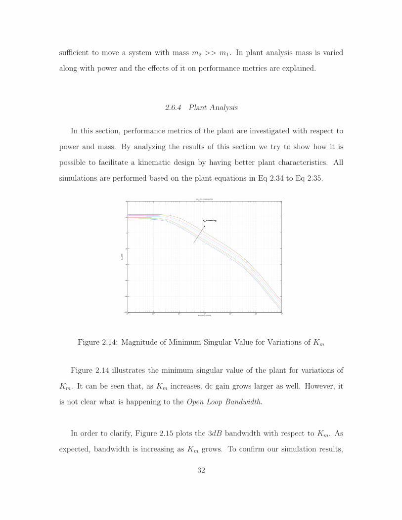
2.14 Magnitude of Minimum Singular Value for Variations of Km . . . . . . . . . . 32

2.15 Open Loop Bandwidth Vs. Km . . . . . . . . . . . . . . . . . . . . . . . . . . . . . . . . . . . . 33

2.16 Magnitude of Diagonal and Off-Diagonal elements for Variations of Km 34

2.17 Magnitude of Off-Diagonal to Diagonal ratio . . . . . . . . . . . . . . . . . . . . . . . . 35

2.18 Cuboid Shape Mobile Robot . . . . . . . . . . . . . . . . . . . . . . . . . . . . . . . . . . . . . . . . 36

2.19 Peak coupling ratio behavior Vs. robot’s aspect ratio . . . . . . . . . . . . . . . . . 37

2.20 Magnitude of Off-Diagonal to Diagonal ratio for Variations of Km . . . . 37

2.21 Magnitude of Minimum Singular Value for Variations of Mass . . . . . . . . . 38

2.22 Open Loop Bandwidth Vs. mass . . . . . . . . . . . . . . . . . . . . . . . . . . . . . . . . . . . 39

2.23 Magnitude of Diagonal and Off-Diagonal elements for Variations of Mass 39

viii

Figure Page

3.1 Decentralized Controller Architecture for Speed Control . . . . . . . . . . . . . . 42

3.2 Magnitude of Diagonal and off-Diagonal elements for variations of K. . . 43

3.3 Minimum singular value for variations of K . . . . . . . . . . . . . . . . . . . . . . . . . . 43

3.4 Bandwidth of the system Vs. Proportional gain (K) . . . . . . . . . . . . . . . . . . 44

3.5 Decentralized Controller Architecture for Speed Control . . . . . . . . . . . . . . 44

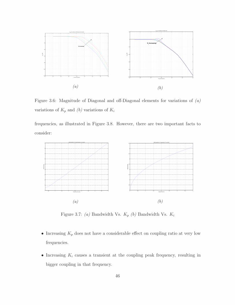
3.6 Magnitude of Diagonal and off-Diagonal elements for variations of (a)

variations of Kp and (b) variations of Ki . . . . . . . . . . . . . . . . . . . . . . . . . . . . . 46

3.7 (a) Bandwidth Vs. Kp (b) Bandwidth Vs. Ki . . . . . . . . . . . . . . . . . . . . . . . . 46

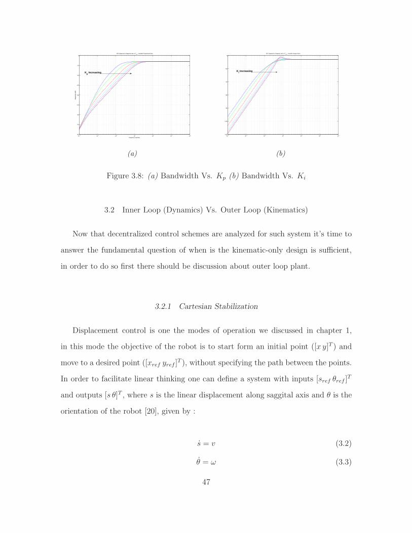
3.8 (a) Bandwidth Vs. Kp (b) Bandwidth Vs. Ki . . . . . . . . . . . . . . . . . . . . . . . . 47

3.9 Displacement Control Block Diagram from Sref and θref to s and θ . . . . 48

3.10 Mobile Robot in Cartesian Stabilization mode . . . . . . . . . . . . . . . . . . . . . . . 48

3.11 Positioning System (Displacement Control) Block Diagram. . . . . . . . . . . . 49

3.12 Error between ideal (Kinematic) and actual (Kinematic + Dynamics)

system Vs. BW ratio . . . . . . . . . . . . . . . . . . . . . . . . . . . . . . . . . . . . . . . . . . . . . . . 50

3.13 (a) max|S12| Vs. BW (b) max|S11| Vs. BW . . . . . . . . . . . . . . . . . . . . . . . . . 51

3.14 |S12

S11| . . . . . . . . . . . . . . . . . . . . . . . . . . . . . . . . . . . . . . . . . . . . . . . . . . . . . . . . . . . . . . 52

3.15 Peak |S12

S11| within BW Vs BW . . . . . . . . . . . . . . . . . . . . . . . . . . . . . . . . . . . . . . 53

3.16 ps Vs. Aspect Ratio . . . . . . . . . . . . . . . . . . . . . . . . . . . . . . . . . . . . . . . . . . . . . . . . 54

3.17 Rule of thumb Vs. Aspect Ratio . . . . . . . . . . . . . . . . . . . . . . . . . . . . . . . . . . . . 54

3.18 Dynamics Plant with a Linear Quadratic Regulator . . . . . . . . . . . . . . . . . . 56

3.19 Closed loop coupling ratio with decentralized control . . . . . . . . . . . . . . . . . 57

3.20 Closed loop coupling ratio with centralized control . . . . . . . . . . . . . . . . . . . 58

ix

Chapter 1

INTRODUCTION

1.1 A Brief History

Contrary to popular belief, Robots are relatively old devices, with Leonardo’s me-

chanical knight dating back to 1495 being the first robot recorded in history [1]. First

major wave of robots started in late 60’s at industrial environments, where manual

labor was gradually being replaced by automated robots in the production lines [2] [3].

The presence of robots in industry have been fortified for many years now; how-

ever, there still remains a huge gap in the market for other types mostly due to

technology limitations and high prices. Recent developments have significantly in-

creased computing capabilities of processors while lowering the costs. This allows

cheap, precise and powerful robots to become a reality in the upcoming years, where

they will only be limited by human imagination.

In 1948 W.Grey Walter designed the first Mobile Robot called Machina Specultrix.

This robot was equipped with a light sensor to explore the environment. Because of

the simple design this machine was extremely unreliable and in need of constant at-

tention [4].

Johns Hopkins University developed the Beast in 1960 utilizing sonar to wander

around the halls until its batteries ran low [5].

1

In 1969 Mowbot was introduced to market where as the first attempt in auto-

matic lawn mowing [6]. In early 90’s Joseph Engelberger, father of industrial robotic

arm, designed the first commercially available autonomous mobile hospital robot [7]

. Later in 1997 NASA sent the Mars Pathfinder with its rover Sojourner to Mars.

Equipped with a hazard avoidance system, Sojourner was able to autonomously find

its way through unknown martian terrain.

Over the past decade the development of mobile robots has faced a new era with

ever increasing processing power of computers along with accurate sensors. In the

past two decades mobile robots, along with their capabilities and their design aspects

have been a very popular topic between scientist from various fields such as controls,

robotics, computer science, etc.

1.2 Literature Sruvey

In this section relevant research will be explored in order to put a foundation for

our work and justify the objective of this document. Although research in this area

has been going on for many years, the most recent articles will be more emphasized.

1.2.1 Main Problems

There are some major problems concerning Mobile Robots which robotic and con-

trol community try to answer. A Mobile Robot, as the name suggests, has to move

from an initial point and reach a final destination, while satisfying speed and/or po-

sition constraints on its way.

2

This task has been broken down into different problems and addressed separately

or together. These problems are classified as:

1. Path Tracking (Trajectory Tracking)

2. Point to Point (Cartesian) Stabilization

3. Posture Regulation (Parking Problem)

4. Velocity Control

Path Tracking is the highest level problem which consists of a robot following a

predefined path and reaching a destination. A more general form of path tracking

is the Trajectory Tracking problem which is proposed by defining a timing law on

the desired path; implicitly putting a velocity constraint on the robot at each sample

point.

One of the most common solutions for this class of problems is through Liapunov-

Like stabilization [8] [9] [10]. In this method a linear or non-linear controller is pro-

posed and the stability of the closed loop system is proved through Liapunov function

[11] [12] [13]. In this approach a non-linear geometric model of mobile robot (Kine-

matics) is incorporated for control design and closed loop stability analysis. [14], [15]

and [16] are some examples of using model predictive controller for trajectory tracking

of nonholonomic systens.

Point to Point stabilization in nature is a simpler problem, where the robot only

has to start from an initial point and reach a destination point. In this class of prob-

lems the behavior of the robot between the initial and final point, and also the final

orientation of the robot is not explicitly controlled. Point to Point stabilization can be

3

addressed as a subclass of Path Tracking or Posture Regulation problems, depending

on the the goal being to follow a path or just reaching a reference point.

Posture regulation is a general form of Point to Point stabilization. The objective

of the robot in this problem is to start from an initial posture and end up at a final

posture. Due to the non-holonomic nature of the system and it limitations, this class

of problems has been recognized as the hardest issues in mobile robotic society.

Liapunov stabilization is the oldest method to solve this problem at kinematic

level [17] [13] [18] [19]. However, recent studies have managed to simplify this prob-

lem by transforming the inputs from posture to displacement and orientation and use

linear controllers to address the problem [20] [21]. This approach not only simplifies

the controller structure, but also allows a more performance based control system

design as well.

Other than [20] and [21], in which the dynamics are included but not explicitly

controlled, all of the previous problems have been addressed in aKinematic level. This

means that the actuator and robot dynamics are neglected and it is assumed that

velocity commands are realized instantaneously. This negligence is justified provided

that the motor is powerful enough or it is already being controlled using lower level

controllers [18] [22] [19] [11] [23]. This brings out the importance of Velocity Control.

Velocity Control of the mobile robot is a very fundamental problem. This is be-

cause underneath any technique addressing the problems mentioned earlier, there is

a need for seamless velocity tracking.

4

In order to achieve this goal different approaches have been proposed. One method

is to cancel the dynamics of the system using state feedback based on the exact knowl-

edge of such dynamics [13], [24], [25]. This method is highly sensitive to the parameter

error and is not considered a very practical approach.

Recent studies have put more focus on the dynamic model and its effects on the

system as a whole. Both the robot and a simplified actuator dynamics have been

considered in [20] and [21]. As it was mentioned earlier, two PID controllers are in-

corporated to solve both path and trajectory problems. In this method the velocity

is not sensed or explicitly controlled. Solely depending on position sensing, which is

in general more prone to errors compared to velocity sensing, can make the system

more susceptible to errors.

In [26] a detailed model of mobile robot including the dynamics and toque cou-

pling has been proposed, the dynamic are then controlled using a Model Reference

Adaptive controller at torque level. Although this is a genuine effort in considering

the dynamics, in most systems commanding torques is not a viable option.

1.3 Objective

From literature survey one can observe while there are many control approaches

for each of the proposed problems, there are gaps in the dynamic modeling aspects of

mobile robots. While all of the surveyed works address the proposed problems, they

are heavily based on assumptions of neglecting the dynamics, which from a control

system design point of view may be unjust.

5

This document explores two major themes : the use of nonlinear kinematic models

for control design and the use of decentralized proportional plus integral (PI) control.

While these topics have received much attention, there still remain critical questions

which have not been rigorously addressed. In this document answers to the following

fundamental questions are provided:

1. When is the Kinematic Model sufficient ?

2. When is the Dynamic Model essential?

3. When is a Decentralized Control scheme sufficient?

4. When is a Centralized Control (MIMO) essential?

The answers to the proposed questions are intended to be used for development of

aMobile Robotic System (MRS) as a part of Flexible Autonomous Machines operating

in an uncertain Environment (FAME) project at Arizona State University.

1.4 Thesis Organization

The remainder of the thesis is organized as follows:

Chapter 2 provides explanations on the mathematical model of a differential drive

mobile robot. In this chapter dynamic and kinematic model are explained along with

non-holonomic constraints of the robot. Additionally, their differences and limita-

tions are thoroughly explored in this chapter. The detailed dynamic model of the

Mobile robot with torque coupling is then introduced. Performance metrics such as

Coupling Ratio and Bandwidth effects of Power and Mass on such system are then an-

alyzed. Finally the dependency of dynamic coupling on the aspect ratio of the robot

is discussed in details. Coupling analysis shows that for a cuboid shape robot with

6

aspect ratio of√5 the coupling goes to zero, allowing for simpler control structures

to be used. At the end by summarizing our analysis we answer how can one design a

system to facilitate a kinematic design, helping with fundamental question 1 and 2.

In Chapter 3, in order to answer the first two previously mentioned fundamental

questions, effects of inner loop system (Dynamics Velocity Loop) on the outer loop

system (Kinematic Position Loop) is compared and a rule of thumb is derived. It’s

concluded that if the Inner loop dynamics is much faster (ten times faster) than the

outer loop kinematics, the error will be small enough, allowing for a kinematic design.

On the other hand if the inner loop dynamics are not fast enough (less than two time

faster than the outer loop) then the error will be large, thus the need for dynamic

model consideration.

Different control schemes for the dynamic model are then analyzed. Decentralized

P and PI controller are designed for such systems and different performance aspects

of such scheme is explored. The limitations of using a decentralized control is then

addressed and a rule of thumb for the third fundamental question is derived. It is

stated that operating in low frequencies, relative to the peak coupling frequency (ωc),

would yield high performance closed loop characteristics. The driven rule of thumb

for the third question is dependent on the aspect ratio of the robot and can become

less strict as we reach the zero coupling aspect ratio of√5.

Finally, it’s shown that if high velocity bandwidth, relative to the peak dynamic

coupling frequency, is desired A Centeralized LQR controller is required. Further

analysis clearly states that the centralized control is able to overcome limitations of

the decentralized scheme, thus allowing us to answer the forth fundamental question.

7

Here, the analysis in the thesis is sparse making the topic an area for future analyt-

ical work

Chapter 4 discusses the outer loop path generation problem of the mobile robot,

focusing on generating viable speed commands for a desired path, which can be ap-

plied to the controlled dynamics discussed in previous chapters.

Chapter 5 summarizes the results in this thesis and proposes the possibility of

future works that hasn’t been addressed in this document.

1.5 Summary and Conclusion

In section 1.1 a brief history of mobile robots was given. Section 1.2 thoroughly

discussed the research that has been done on mobile robots, addressing main problems

of the field. In section 1.3 the main objective of this thesis, and the reasoning behind

it was proposed. Finally section 1.4 showed how the rest of this thesis is organized

and what is discussed in each chapter.

8

Chapter 2

MATHEMATICAL MODEL

Deriving a precise mathematical model is a crucial part of designing control sys-

tem for any physical plants such as mobile robots. In this chapter dynamics and

kinematics of a differential drive robot are derived and differences between the two

models and limitations of the kinematic model are explored.

The pure rolling nature of the wheels causes a reduction in the local mobility of

the robot. This limitation is expressed as a non-holonomic constraint which is fur-

ther discussed. In later chapters the importance of the non-holonomic constraint in

trajectory planning is thoroughly discussed.

2.1 Non-Holonomic Constraint

Wheeled vehicles are generally subjected to a constraint. For instance, a car can

reach any final configuration in its plane, but it can never move sideways. Hence, de-

pending on the goal configuration, it requires to perform a series of maneuvers (such

as parallel parking) to reach the desired state.

First, holonomic and non-holonomic systems have to be defined. Let’s consider a

mechanical system with generalized coordinates q ∈ C, where C is the configuration

space of the proposed system and coincides with Rn. For such system, a constraint is

called Kinematic when it only involves generalized coordinates (q) and velocities (q).

9

Kinematic Constraints are usually defined in Pfaffian Form

vTi (q)q = 0 i = 1, ..., k < n (2.1)

where vi’s are k linearly independent vectors.

If all of the kinematic constraints defined by Equation 2.10 are integrable to a

form of

hi(q) = mi i = 1, ..., k < n

where, mi is the integration constant, then they are considered to be holonomic con-

straints and the system subjected to them is called a holonomic system. Joints in a

robotic manipulator are common example of such constraints.

Each holonomic constraint causes a loss of accessibility of the system in its con-

figuration space. Hence, for a system with k holonomic constraints, the accessible

configurations are reduced to a n− k dimensional subset of C.

A non-holonomic system on the other hand, is subjected to at least one non-

integrable (i.e. non-holonomic) constraint. Although such constraint limits the local

mobility of the system, due to its non-integrable nature, the accessibility to C is

not affected. Hence, generalized coordinates are not reduced. However, generalized

velocities in a system subjected to k non-holonomic constraint belongs to a (n − k)

dimensional subspace.

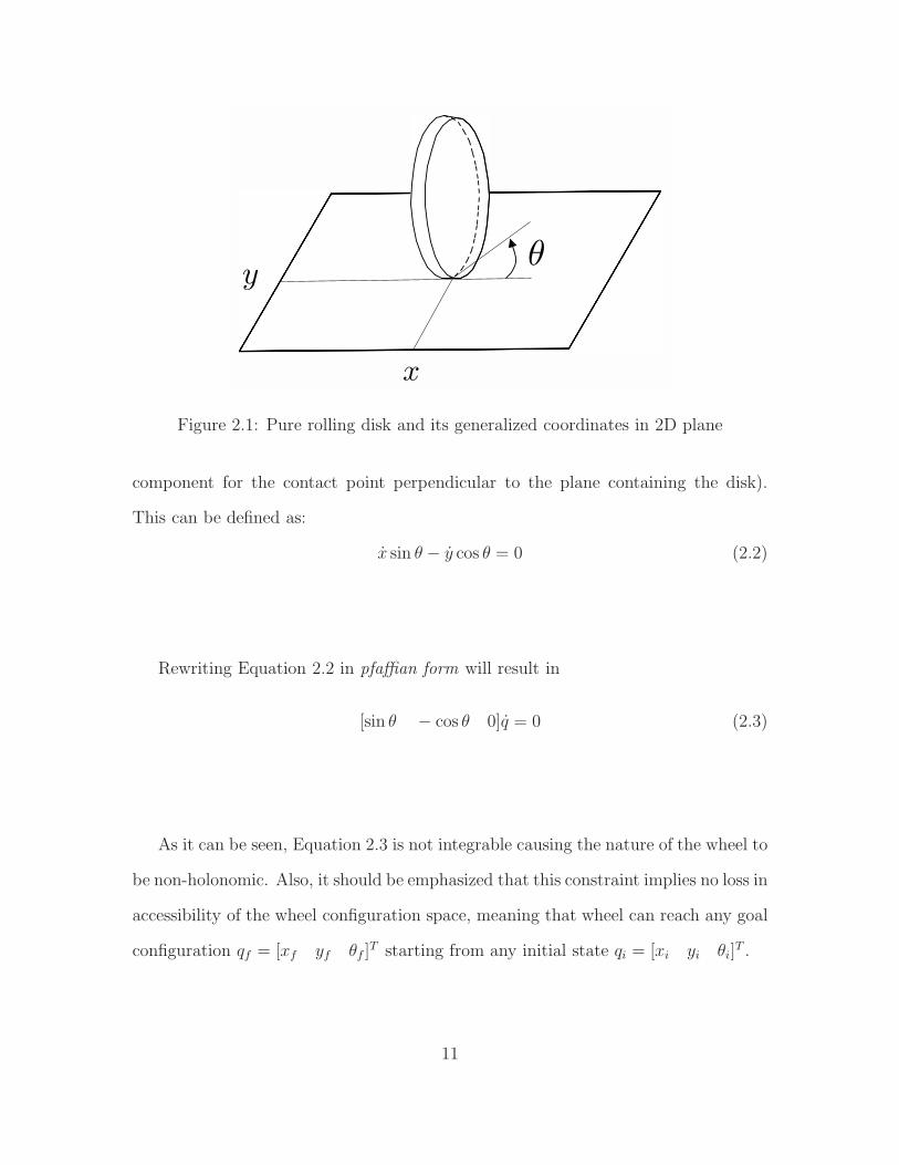
Wheels are typical sources of non-holonomic constraints. Consider the disk in

Figure 2.1 with generalized coordinates q = [x y θ]T , assuming the disk can only

roll on the touching plane without slipping to the sides (i.e. there is no velocity

10

x

yθ

Figure 2.1: Pure rolling disk and its generalized coordinates in 2D plane

component for the contact point perpendicular to the plane containing the disk).

This can be defined as:

x sin θ − y cos θ = 0 (2.2)

Rewriting Equation 2.2 in pfaffian form will result in

[sin θ − cos θ 0]q = 0 (2.3)

As it can be seen, Equation 2.3 is not integrable causing the nature of the wheel to

be non-holonomic. Also, it should be emphasized that this constraint implies no loss in

accessibility of the wheel configuration space, meaning that wheel can reach any goal

configuration qf = [xf yf θf ]T starting from any initial state qi = [xi yi θi]

T .

11

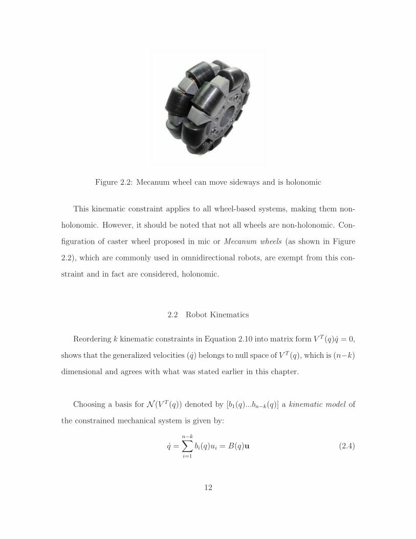
Figure 2.2: Mecanum wheel can move sideways and is holonomic

This kinematic constraint applies to all wheel-based systems, making them non-

holonomic. However, it should be noted that not all wheels are non-holonomic. Con-

figuration of caster wheel proposed in mic or Mecanum wheels (as shown in Figure

2.2), which are commonly used in omnidirectional robots, are exempt from this con-

straint and in fact are considered, holonomic.

2.2 Robot Kinematics

Reordering k kinematic constraints in Equation 2.10 into matrix form V T (q)q = 0,

shows that the generalized velocities (q) belongs to null space of V T (q), which is (n−k)

dimensional and agrees with what was stated earlier in this chapter.

Choosing a basis for N (V T (q)) denoted by [b1(q)...bn−k(q)] a kinematic model of

the constrained mechanical system is given by:

q =

n−k∑

i=1

bi(q)ui = B(q)u (2.4)

12

where u = [u1...un−k]T ∈ R

n−k is the input vector and q ∈ Rn is the state vector.

The basis for nullspace of V T (q) is not unique and typically, it can be chosen such

that inputs ui represent a physical concept. However, these inputs should not directly

represent forces or torques, hence the name kinematic model.

c.g

x

∠θ

y

Figure 2.3: Generalized coordinates for a mobile robot

Consider the mobile robot in Figure 2.3. Using generalized coordinate vector

q = [x y θ] the robot’s posture can be defined on its whole configuration space.

The wheels driving the robot make it non-holonomic and imposes the pure rolling

constraint on the system which as discussed before, is expressed as

V T (q)q = [sin θ − cos θ 0]q = 0 (2.5)

13

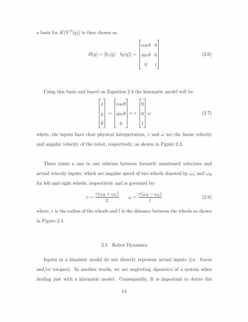
a basis for N (V T (q)) is then chosen as

B(q) = [b1(q) b2(q)] =

cos θ 0

sin θ 0

0 1

(2.6)

Using this basis and based on Equation 2.4 the kinematic model will be

x

y

θ

=

cos θ

sin θ

0

v +

0

0

1

ω (2.7)

where, the inputs have clear physical interpretation, v and ω are the linear velocity

and angular velocity of the robot, respectively, as shown in Figure 2.3.

There exists a one to one relation between formerly mentioned velocities and

actual velocity inputs, which are angular speed of two wheels denoted by ωL and ωR

for left and right wheels, respectively and is governed by:

v =r(ωR + ωL)

2ω =

r(ωR − ωL)

l(2.8)

where, r is the radius of the wheels and l is the distance between the wheels as shown

in Figure 2.4.

2.3 Robot Dynamics

Inputs in a kinamtic model do not directly represent actual inputs (i.e. forces

and/or torques). In another words, we are neglecting dynamics of a system when

dealing just with a kinematic model. Consequently, It is important to derive the

14

ω

v

l

ωR

r

Figure 2.4: Linear and Angular velocity of the robot

dynamic model and explore its characteristics.

There are two methods for dynamic model derivation. Newton-Euler method de-

scribes the system in terms of all the forces and momentum acting on the system

based of direct interpretations of Newtons Second Law of Motion.

On the other hand, Lagrange method incorporates the concepts of Work and En-

ergy to indirectly derive the equations of motion. Here, Lagrange method is chosen

due to its more systematic nature and automatic elimination of workless and con-

straint forces.

Lagrangian of a system is defined as the difference between its kinetic and poten-

tial energy

15

L(q, q) = T (q, q)− U(q) = 1

2qT I(q)q − U(q) (2.9)

where, T (q, q) and U(q) are the kinetic and potential energy, respectively and I(q) is

the inertia matrix of the mechanical system.

Lagrange-Euler equations representing the dynamics are expressed as

d

dt

(

∂L∂q

)T

−(

∂L∂q

)T

= 0 (2.10)

This general form of Lagrange equation applies to holonomic system. In case of a

non-holonomic system we have to replace Equation 2.10 by

d

dt

(

∂L∂q

)T

−(

∂L∂q

)T

= S(q)τ + V (q)λ (2.11)

where, S(q) is a (n by m) matrix mapping the (m = n − k) external inputs τ to

generalized forces, V (q) is the transpose of V T (q) in Equation 2.5 governing the non-

holonomic constraint. λ ∈ Rm is the vector of the Lagrange multipliers representing

the forces required to impose such constraint in the configuration plane. V (q)λ is the

reaction forces at generalized coordinate plane.

Based on Equation 2.9 and Equation 2.10, the dynamical model of a non-holonomic

mechanical system is obtained as

I(q)q + n(q, q) = S(q)τ + V (q)λ (2.12)

V T (q)q = 0 (2.13)

n(q, q) = I(q)q − 1

2

(

∂

∂q(qT I(q)q)

)T

+

(

∂U(q)∂q

)T

(2.14)

16

where n(q, q) given in Eq 2.14 represents vector of centripetal and coriolis terms [26]

[27].

Let I be the moment of inertia around the central vertical axis and m the mass

of the differential drive mobile robot in 2.3. Using the Lagrange representation in

Equation 2.12 and Equation 2.13, the dynamic model of the robot is then derived.

m 0 0

0 m 0

0 0 I

x

y

θ

=

cos θ 0

sin θ 0

0 1

τl

τa

+

sin θ

− cos θ

0

λ (2.15)

[

sin θ − cos θ 0

]

q = 0 (2.16)

Where, τl and τa represent the linear force and angular torque of the mobile robot,

respectively. The robot is in inertial frame coriolis and centripetal term n(q, q) is

non-existence [26].

The relations between linear velocity (v), angular velocity (ω) and the generalized

velocities (q) are

v =√

x2 + y2 (2.17)

ω = θ (2.18)

Using derivatives of Equation 2.17 and Equation 2.18, the dynamic model represented

in matrix form in Equation 2.15 can be rewritten in a more familiar form.

17

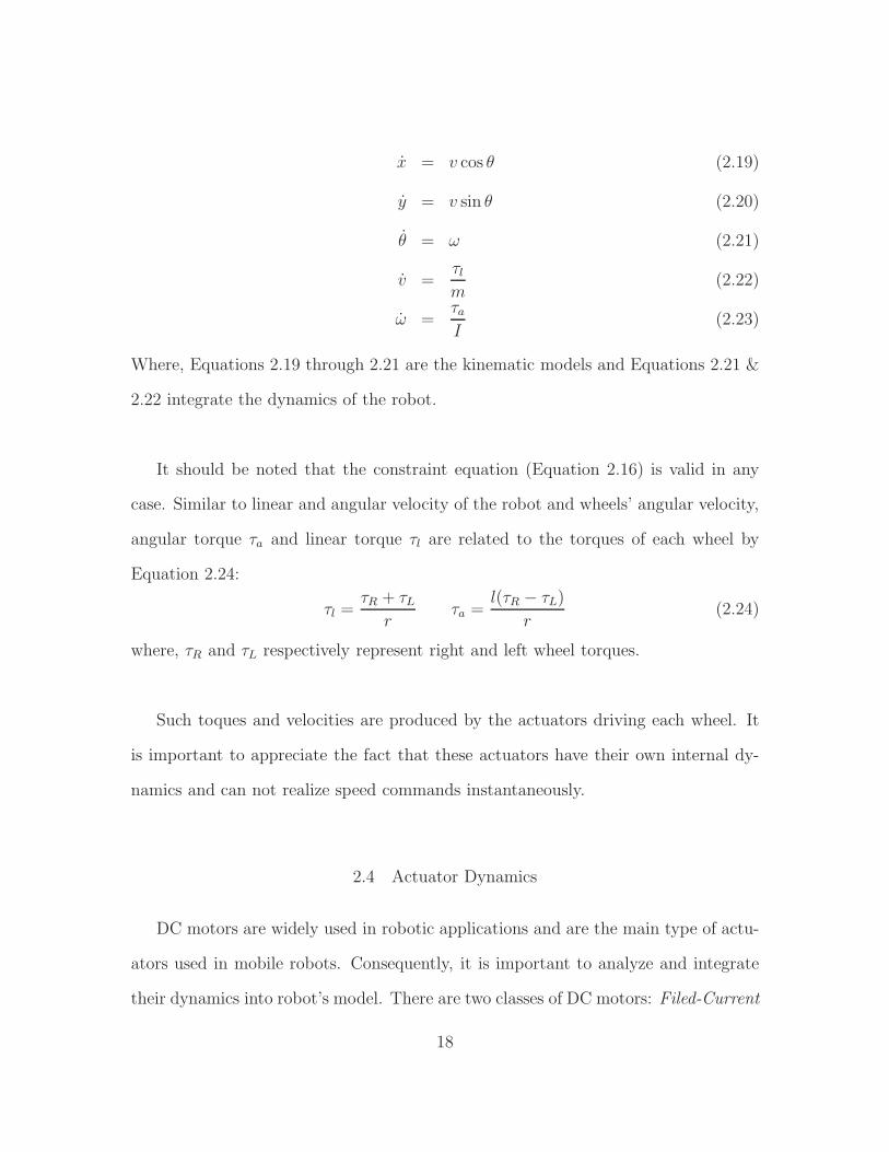
x = v cos θ (2.19)

y = v sin θ (2.20)

θ = ω (2.21)

v =τlm

(2.22)

ω =τaI

(2.23)

Where, Equations 2.19 through 2.21 are the kinematic models and Equations 2.21 &

2.22 integrate the dynamics of the robot.

It should be noted that the constraint equation (Equation 2.16) is valid in any

case. Similar to linear and angular velocity of the robot and wheels’ angular velocity,

angular torque τa and linear torque τl are related to the torques of each wheel by

Equation 2.24:

τl =τR + τL

rτa =

l(τR − τL)

r(2.24)

where, τR and τL respectively represent right and left wheel torques.

Such toques and velocities are produced by the actuators driving each wheel. It

is important to appreciate the fact that these actuators have their own internal dy-

namics and can not realize speed commands instantaneously.

2.4 Actuator Dynamics

DC motors are widely used in robotic applications and are the main type of actu-

ators used in mobile robots. Consequently, it is important to analyze and integrate

their dynamics into robot’s model. There are two classes of DC motors: Filed-Current

18

Controlled and Armature-Current Controlled. In a Field-Current Controlled motor,

the armature current ia is kept constant while the field-current is controlled using

field voltage Vf commands.

On the other hand, in a Armature-Current Controlled motor, the armature volt-

age Va is the command to control the armature current while keeping the field-current

if constant. Armature-current controlled DC motors are more common choice in mo-

bile robots and are the basis of further discussions in this text. For a more detailed

discussion on DC motor modeling refer to [28], [29] and [30].

_

+

Ra La

ev

+

-

Fixed

field

ia

τ

cω

J

Figure 2.5: Circuit equivalent of a DC motor with a free body attached

In an Armature-Current Controlled structure, the motor torque is linearly depen-

dent on the armature current by

τm(s)

Ia(s)= Km (2.25)

19

where, τm(s) is the motor torque in S-domain and Km is called the motor torque

constant.

Based on circuit model provided in Figure 2.5, and considering the back EMF

voltage (vb), induced by the rotation of armature winding, the voltage relation on the

armature will be

va = vr + vL + vb (2.26)

Back EMF has a linear relation to angular speed through back EMF constant Kb,

taking Laplace transform of Equation 2.26 the following equation is achieved.

Va(s)− Vb(s) = Va(s)−Kb ω(s) = (Ra + Las)Ia(s) (2.27)

θ

τm cθ = cω

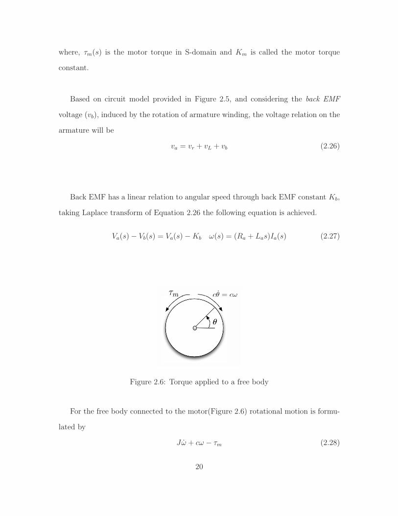
Figure 2.6: Torque applied to a free body

For the free body connected to the motor(Figure 2.6) rotational motion is formu-

lated by

Jω + cω − τm (2.28)

20

where, ω is the angular velocity, c is motor friction constant and J is the moment of

inertia of the rotor.

Taking Laplace transform the transfer function from the input motor torque to

angular velocity is obtained

ω(s)

Tm(s)=

1

J.s+ c(2.29)

Using Equations 2.25,2.27 and 2.29 transfer function from armature voltage to

angular velocity is

ω(s)

Va(s)=

Km

(La.s+Ra)(Js+ c) +KbKm

(2.30)

Closed loop block diagram of DC motor model expressed in Equation 2.30 is shown

in Figure 2.7, angular displacement can also be found by integrating ω(s).

+-

1

Las+Ra

Va(s) Ia(s) Tm(s)

Km

ω(s)1

Js+ c

Kb

Figure 2.7: DC Motor block diagram

21

2.5 Kinematics Vs. Dynamics

In previous sections kinematics and dynamics of a differential drive mobile robot

was systematically derived. In robotic society it is very common to use the kine-

matic model as the plant for control design [13] [18] [31] [12] [19]. This is justified

by assuming that the motor is powerful enough to make the dynamic effects negligible.

This section is intended to have a deeper look into this matter by comparing the

kinematic and dynamic model and exploring the limitations of the kinematic model.

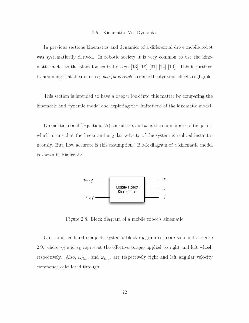
Kinematic model (Equation 2.7) considers v and ω as the main inputs of the plant,

which means that the linear and angular velocity of the system is realized instanta-

neously. But, how accurate is this assumption? Block diagram of a kinematic model

is shown in Figure 2.8.

Mobile Robot

Kinematics

x

y

θ

vref

ωref

Figure 2.8: Block diagram of a mobile robot’s kinematic

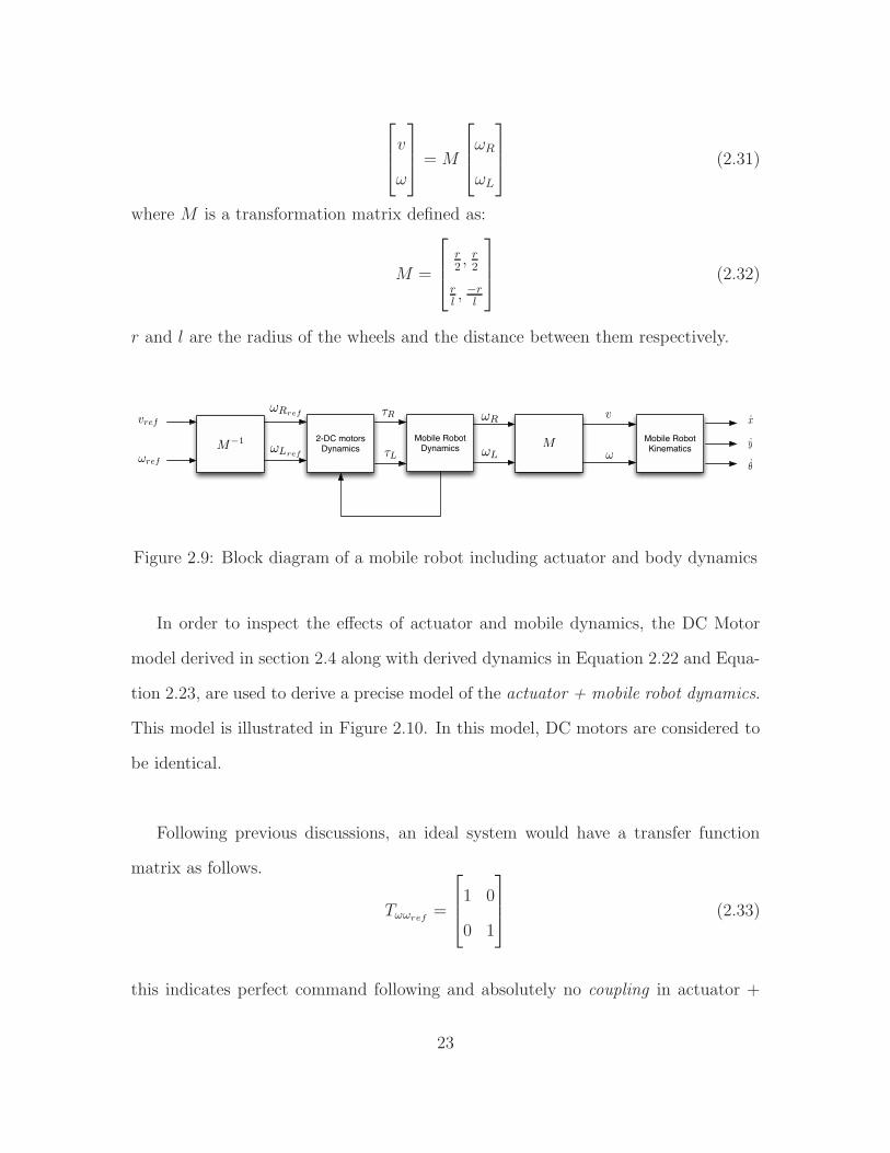
On the other hand complete system’s block diagram so more similar to Figure

2.9, where τR and τL represent the effective torque applied to right and left wheel,

respectively. Also, ωRrefand ωLref

are respectively right and left angular velocity

commands calculated through:

22

v

ω

= M

ωR

ωL

(2.31)

where M is a transformation matrix defined as:

M =

r2, r2

rl, −r

l

(2.32)

r and l are the radius of the wheels and the distance between them respectively.

x

y

θ

vref

ωrefτL

τR v

ω

2-DC motors Dynamics

ωRref

ωLref ωL

ωR

Mobile Robot Dynamics

Mobile Robot KinematicsM

−1 M

Figure 2.9: Block diagram of a mobile robot including actuator and body dynamics

In order to inspect the effects of actuator and mobile dynamics, the DC Motor

model derived in section 2.4 along with derived dynamics in Equation 2.22 and Equa-

tion 2.23, are used to derive a precise model of the actuator + mobile robot dynamics.

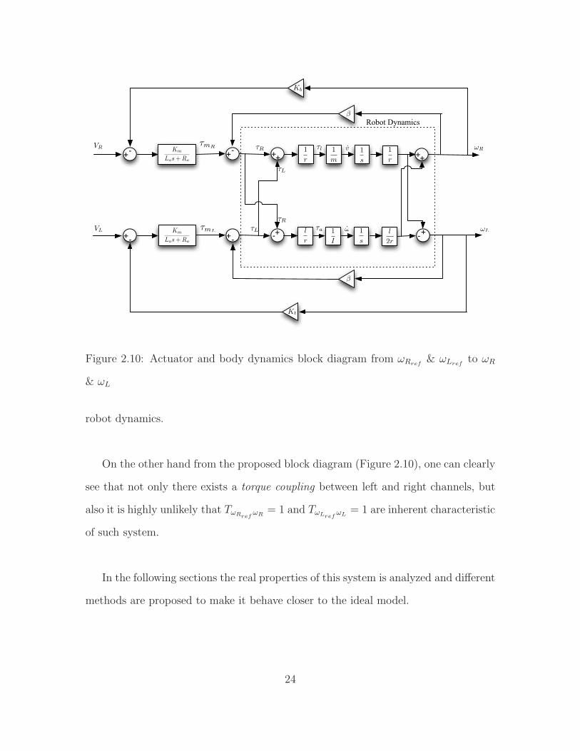
This model is illustrated in Figure 2.10. In this model, DC motors are considered to

be identical.

Following previous discussions, an ideal system would have a transfer function

matrix as follows.

Tωωref=

1 0

0 1

(2.33)

this indicates perfect command following and absolutely no coupling in actuator +

23

τl

+- Km

Las+Ra

+-

++

+-+

-

Km

Las+Ra

+-

τR

τL

1

s

1

r

++

+1

s

l

r

1

I

l

2r-

τL

τR

τa

1

m

1

r

v

ω

β

Kb

Kb

β

VR

VL

ωR

ωL

τmR

τmL

Robot Dynamics

Figure 2.10: Actuator and body dynamics block diagram from ωRref& ωLref

to ωR

& ωL

robot dynamics.

On the other hand from the proposed block diagram (Figure 2.10), one can clearly

see that not only there exists a torque coupling between left and right channels, but

also it is highly unlikely that TωRrefωR

= 1 and TωLrefωL

= 1 are inherent characteristic

of such system.

In the following sections the real properties of this system is analyzed and different

methods are proposed to make it behave closer to the ideal model.

24

2.6 Robot + Actuator Dynamics

In this section, properties of the actuator + robot dynamics will be discussed in

more details. For a system shown in 2.9 one can derive equations as expressed Eq

2.34 to Eq 2.35:

v

ω

= Jm2×2T2×2Km2×2i− Jm2×2T2×2β2×2ωw (2.34)

i = −L2×2R2×2i− L2×2K2×2ωw + L2×2V (2.35)

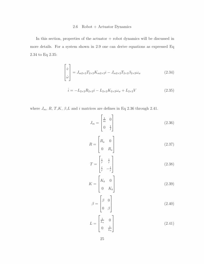
where Jm, R, T ,K, β,L and i matrices are defines in Eq 2.36 through 2.41.

Jm =

1m

0

0 1I

(2.36)

R =

Ra 0

0 Ra

(2.37)

T =

1r

1r

lr

− lr

(2.38)

K =

Kb 0

0 Kb

(2.39)

β =

β 0

0 β

(2.40)

L =

1La

0

0 1La

(2.41)

25

i =

ia1

ia2

(2.42)

Assuming La ≈ 0,one can approximate the transfer function matrix of the system

shown in Fig 2.10 as

Pωv =

Pωv11 Pωv12

Pωv21 Pωv22

(2.43)

where,

Pωv11 = Pωv22 ≈a(s+ z1)

(s+ p1)(s+ p2)(2.44)

Pωv12 = Pωv21 ≈ds

(s+ p1)(s+ p2)(2.45)

Gains, poles and zeros are approximately located at

a =Km

JLa

(2.46)

d =Km(J2 − J1)

J1J2La

(2.47)

p1 ≈2(Raβ +KbKm)

RaJ1(2.48)

p2 ≈2(Raβ +KbKm)

RaJ2(2.49)

z1 ≈(Raβ +KbKm)

RaJ2

(2.50)

26

where, J, J1 and J2 are inertial parameters which are used to model mass and inertia

of the robot. These parameters are expressed as

J =J1J2

J1 + J2=

2Imr2

2I + l2m(2.51)

J1 = mr2 (2.52)

J2 =2r2I

l2(2.53)

Table 2.1 describes the physical representation of each parameter along with the

nominal value of them. Further numerical calculations and simulations are based

upon the nominal plant.

Figure 2.11 and Figure2.12, respectively depict the Singular value and Bode plot

of Pd.

From Figure 2.12 one can easily conclude that, depending on the application,

neglecting the dynamics can have drastic outcomes. Before proceeding further, per-

formance metrics have to be selected to assist us in in-depth analysis of the plant.

2.6.1 Plant Characteristics

In general, when designing and analyzing a system, one needs to satisfy a perfor-

mance goal or goals. These goals are quantified using performance metrics. Based on

27

Table 2.1: Dynamic Model Parameter Description and their Nominal Values

Parameter Description Nominal Value

Km Torque Constant 0.0487 N.m/Amp

La Armature Inductance 0.64× 10−3 H

Ra Armature Resistance 0.27 ohm

r Wheel Raduis 0.1 m

m Mass 30 Kg

I Interia 0.83 Kg.m2

l Distance between the wheels 0.5 m

β Friction Constant 0.021 N.m.s

Kb Back EMF Constant 0.0487 V/(rad/sec)

10−2

10−1

100

101

102

103

104

−120

−100

−80

−60

−40

−20

0

20

Singular Values of the 2 Motor channels, Robot’s dynamics included

Frequency (rad/s)

Sin

gula

r V

alue

s (d

B)

σmin

σmax

Figure 2.11: Singular Value plot of Mobile Robot Dynamics

previous discussions, we need this system to look close to I2x2. This means there are

two important factors to consider:

• Bandwidth

28

−120

−100

−80

−60

−40

−20

0

20From: v1

To:

ω1

10−2

10−1

100

101

102

103

104

−120

−100

−80

−60

−40

−20

0

20

To:

ω2

From: v2

10−2

10−1

100

101

102

103

104

Bode Diagram

Frequency (rad/s)

Mag

nitu

de (

dB)

Figure 2.12: Bode Magnitude Plot of Mobile Robot Dynamics

• Coupling

Bandwidth is a measure of system’s speed, larger bandwidth generally means

less response time. In other words, Bandwidth measures the frequency range at which

the system behaves close to a constant, and is easier to be controlled.

Bandwidth can have different definitions based on the case. In this document,

3dB Bandwidth of plant’s minimum Singular Value will be used as a performance

metric which is defined as:

|σmin(ω3dB)| =|σmin(0)|√

2(2.54)

29

Coupling is the behavior of the off-diagonal elements in the transfer function

matrix, while it is not considered as a metric by itself. However, it is crucial for it to

get quantified.

Based on bode plot of the system (Figure 2.12) it is clear that this system has

small coupling at low and high frequencies with a peak in the middle. As discussed

before, ideally this term has to be small compared to the diagonal term, which justifies

using the following ratio as a measure of coupling.

Cratio =|P12(ω)||P11(ω)|

(2.55)

In this equation, smaller Cratio means smaller coupling, thus better plant char-

acteristics. It should be noted that each of these metrics can have slightly different

meaning for different type of systems. A desirable plant, would be a system with high

bandwidth and small coupling. In following sections designing a robot with desirable

characteristics is discussed in details.

2.6.2 Power

It was previously mentioned that it is common for robotic scientists to neglect

robot and actuator dynamics based on the concept that Motors are powerful enough.

In order to have an in depth discussion about this statement, Power should be defined

in terms of motor parameters. Using DC-Motor model derived in Section 2.4, dc power

can be derived as

P (0) = τ(0)ω(0) (2.56)

30

0 0.01 0.02 0.03 0.04 0.05 0.06 0.07 0.08 0.09 0.10

200

400

600

800

1000

1200Motor Power Vs. Torque Constant

Km (N.m/Amp)

Pow

er (

Wat

ts)

Figure 2.13: Variation of Power Vs. Km

where,

τ(0) =Kmβ

βRa +KmKb

× Va (2.57)

ω(0) =Km

βRa +KmKb

× Va (2.58)

τ(0) and ω(0) represent the dc torque and speed of the motor, respectively. Ac-

cording to these equations, it is obvious that Km has direct effect on the power. For

further analysis, Km is used as a mean to manipulate power’s value. Figure 2.13

shows the relation between power and Km for this motor.

2.6.3 Mass

The discussion of power is incomplete without considering mass. While a motor

is considered powerful for a system with mass m1, it may not be powerful, or even

31

sufficient to move a system with mass m2 >> m1. In plant analysis mass is varied

along with power and the effects of it on performance metrics are explained.

2.6.4 Plant Analysis

In this section, performance metrics of the plant are investigated with respect to

power and mass. By analyzing the results of this section we try to show how it is

possible to facilitate a kinematic design by having better plant characteristics. All

simulations are performed based on the plant equations in Eq 2.34 to Eq 2.35.

10−2

10−1

100

101

102

103

104

−100

−80

−60

−40

−20

0

20

40

Frequency (rad/sec)

|σm

in|(

dB)

|σmin

| for variations of Km

Km

increasing

Figure 2.14: Magnitude of Minimum Singular Value for Variations of Km

Figure 2.14 illustrates the minimum singular value of the plant for variations of

Km. It can be seen that, as Km increases, dc gain grows larger as well. However, it

is not clear what is happening to the Open Loop Bandwidth.

In order to clarify, Figure 2.15 plots the 3dB bandwidth with respect to Km. As

expected, bandwidth is increasing as Km grows. To confirm our simulation results,

32

0 0.05 0.1 0.15 0.2 0.25 0.3 0.35 0.4 0.450.2

0.3

0.4

0.5

0.6

0.7

0.8

0.9

1

1.1

1.2

Km

3dB

Ban

dwid

th o

f |σ m

in|

Plant Bandwidth Vs. Km

Figure 2.15: Open Loop Bandwidth Vs. Km

the open loop bandwidth has been calculated analytically in Equation 2.59.

BW3dB(σmin) ≈2(Raβ +KbKm)

RaJ1(2.59)

This confirms that open loop bandwidth increases linearly with Km.

Plotting the Diagonal with respect to Off Diagonal elements of Pd, as shown Fig-

ure 2.16, provides more insight into how the plant behaves. The off-diagonal peak

moves further into higher frequencies as Km increases. This means a larger frequency

range of small coupling behavior, which is desirable.

The diagonal and off diagonal elements have exactly similar poles, which means

they will have similar behavior in a particular frequency range. This confirms the

33

10−2

10−1

100

101

102

103

104

−100

−80

−60

−40

−20

0

20

40

From: v1 To: ω1

Mag

nitu

de (

dB)

Bode Diagram

Frequency (rad/s)

As Km

gets bigger, |Tv

1ω

1

| gets bigger

As Km

gets bigger, ωc increases

At low frequencys diagonal/off diagonal gets bigger as Km increases

Figure 2.16: Magnitude of Diagonal and Off-Diagonal elements for Variations of Km

importance of choosing Coupling Ratio as a metric.

2.6.5 Robot Aspect Ratio

Figure 2.17 plots the coupling ratio with Vs. frequency for the nominal plant. As

it can be seen in this figure, the ratio grows to a constant peak as frequency increases.

The coupling ratio is calculated as

Cratio =

∣

∣

∣

∣

Pωv11

Pωv12

∣

∣

∣

∣

=

∣

∣

∣

∣

g1s+ z1

s

∣

∣

∣

∣

(2.60)

|g1| =∣

∣

∣

∣

J2 + J1

J2 − J1

∣

∣

∣

∣

(2.61)

where, the peak happens at ωc .

34

10−2

10−1

100

101

102

103

104

−40

−35

−30

−25

−20

−15

−10

−5

Diagonal to Off−Diagonal ratio of Tω v

frequency (rad/sec)

Cra

tio

Figure 2.17: Magnitude of Off-Diagonal to Diagonal ratio

The peak value of coupling ratio is defined in Equation 2.61, where it is dependent

on the inertial parameters of the system J1 and J2. Substituting inertial parameters

into |g1|, the peak can be derived as

|g1| =∣

∣

∣

∣

∣

2Il2−m

2Il2+m

∣

∣

∣

∣

∣

(2.62)

It is observed that coupling peak is dependent on mass, inertia and distance

between the wheels. In order to gain more insight let’s consider the simple mobile

robot in Figure 2.18. Assuming an absolute cuboid with length d and width w, Inertia

around the z axis is then calculated by

I =m

12(w2 + d2) (2.63)

35

Figure 2.18: Cuboid Shape Mobile Robot

Assuming the distance between the wheels is almost equal to the robot width

(l ≈ w), by substituting I from Equation 2.63 into 2.62, |g1| can be calculated as :

|g1| =∣

∣

∣

∣

−5w2 + d2

7w2 + d2

∣

∣

∣

∣

(2.64)

which shows the dependency of peak coupling on the structure of the robot, more

specifically the aspect ratio of the robot. The aspect ratio of the robot is defined as :

robot aspect ratio (RAR) =d

w(2.65)

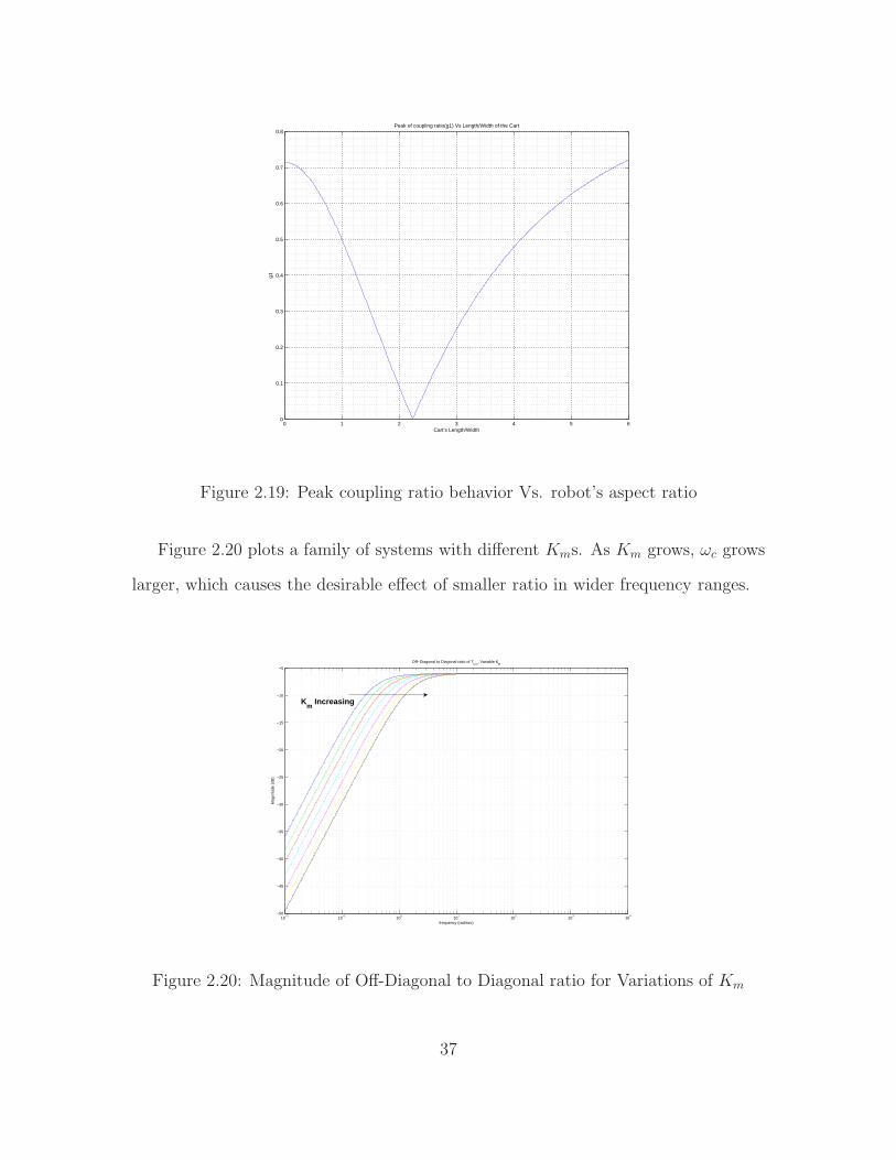
Fig 2.19 depicts how peak coupling changes as we change the aspect ratio. As

the aspect ratio grows, peak coupling reaches 0 at dw=

√5, and as we deviate from

this point the peak grows to larger values. This means an aspect ratio of√5 would

ensure zero coupling for the robot, assuming the robot has an absolute cuboid shape

of course.

36

0 1 2 3 4 5 60

0.1

0.2

0.3

0.4

0.5

0.6

0.7

0.8Peak of coupling ratio(g1) Vs Length/Width of the Cart

Cart’s Length/Width

g1

Figure 2.19: Peak coupling ratio behavior Vs. robot’s aspect ratio

Figure 2.20 plots a family of systems with different Kms. As Km grows, ωc grows

larger, which causes the desirable effect of smaller ratio in wider frequency ranges.

10−2

10−1

100

101

102

103

104

−50

−45

−40

−35

−30

−25

−20

−15

−10

−5

Off−Diagonal to Diagonal ratio of Tω v, Variable K

m

frequency (rad/sec)

Mag

nitu

de (

dB)

Km

Increasing

Figure 2.20: Magnitude of Off-Diagonal to Diagonal ratio for Variations of Km

37

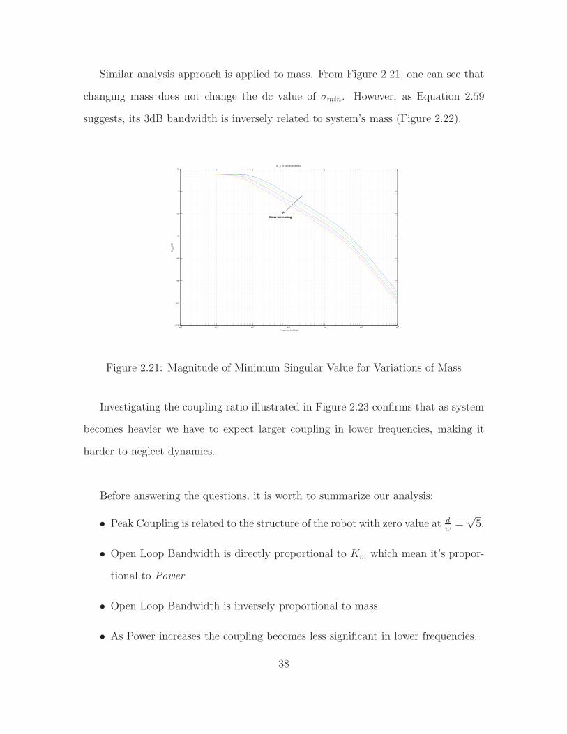
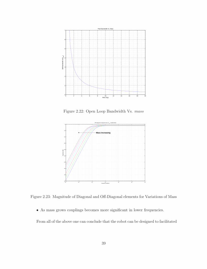
Similar analysis approach is applied to mass. From Figure 2.21, one can see that

changing mass does not change the dc value of σmin. However, as Equation 2.59

suggests, its 3dB bandwidth is inversely related to system’s mass (Figure 2.22).

10−2

10−1

100

101

102

103

104

−120

−100

−80

−60

−40

−20

0

20

Frequency (rad/sec)

|σm

in|(

dB)

|σmin

| for variations of Mass

Mass Increasing

Figure 2.21: Magnitude of Minimum Singular Value for Variations of Mass

Investigating the coupling ratio illustrated in Figure 2.23 confirms that as system

becomes heavier we have to expect larger coupling in lower frequencies, making it

harder to neglect dynamics.

Before answering the questions, it is worth to summarize our analysis:

• Peak Coupling is related to the structure of the robot with zero value at dw=

√5.

• Open Loop Bandwidth is directly proportional to Km which mean it’s propor-

tional to Power.

• Open Loop Bandwidth is inversely proportional to mass.

• As Power increases the coupling becomes less significant in lower frequencies.

38

0 2 4 6 8 10 12 14 16 18 200

1

2

3

4

5

6

7

Mass (Kg)

3dB

Ban

dwid

th o

f |σ m

in|

Plant Bandwidth Vs. Mass

Figure 2.22: Open Loop Bandwidth Vs. mass

10−2

10−1

100

101

102

103

104

−50

−45

−40

−35

−30

−25

−20

−15

−10

−5

Off−Diagonal to Diagonal ratio of Tω v, Variable Mass

frequency (rad/sec)

Mag

nitu

de (

dB)

Mass Increasing

Figure 2.23: Magnitude of Diagonal and Off-Diagonal elements for Variations of Mass

• As mass grows couplings becomes more significant in lower frequencies.

From all of the above one can conclude that the robot can be designed to facilitated

39

a kinematic control design, more power, smaller mass and an optimum aspect ratio

is all that is needed.

2.7 Conclusion

In this chapter, mathematical modelling of a differential drive mobile robot was

discussed. Furthermore, the differences and limitations of both dynamic and kine-

matic models were explained. The detailed dynamic model of the Mobile robot with

torque coupling is then introduced followed by the effects of power,mass and aspect

ratio of the robot on Bandwidth and coupling characteristics of the plant. Finally,

using all this discussion it’s addressed how can one design a mobile robot system to

facilitate kinematic control design.

40

Chapter 3

DYNAMICS CONTROL DESIGN

This chapter is dedicated to address the control of the Mobile Robot Dynamics (Inner

Loop). Decentralized control architecture based on P and PI controllers is proposed

and applied to the Dynamics plant. One mode of the outer loop is briefly discussed,

allowing us to analyze the relation between the inner loop (Dynamics) and outer loop

(Kinematics). Analyzing such relation results in answering the first two fundamental

questions:

1. When is the Kinematic model sufficient?

2. When is the Dynamic model essential?

In section 3.3 the limitation of a decentralized control architecture is exposed, and

a rule of thumb based on the aspect ratio of the robot is derived, hence answering

the third fundamental question : ” When is the Decentralized control sufficient?”.

Finally a centralized control architecture ( LQR ) is proposed and implemented,

confirming that it’s possible to overcome decentralized control limitations using cen-

tralized scheme. maximum error

3.1 Decentralized Control

In this section different schemes of decentralized controller are implemented in

order to control the dynamic plant of the mobile robot. The block diagram of such

implementation is shown in Figure 3.1.

41

The plant (2-DC motors + Mobile Robot Dynamics) is governed by Eq 2.34 to

Eq 2.35 through out the whole chapter, the controller is specifically defined in each

section.

2-DC motors + Mobile Robot

Dynamics

+-

+-

ωRref

ωLref

C1

ωR

ωLC2

Figure 3.1: Decentralized Controller Architecture for Speed Control

Ideally the motors on the robot are identical, which justifies for C1 and C2 to be

equal to each other.

3.1.1 Proportional Controller

Proportional or P Controller is the simplest form of decentralized control, where

C1 = C2 = K and K is just a gain. Figure 3.2 plots how the diagonal and off diagonal

elements of Tωrefω change as the proportional gain changes, as K increases:

• Steady state error decreases .

• Peak of the off-diagonal element moves to higher frequencies.

• Off-diagonal element gets smaller in lower frequencies.

As it can be seen in Figure 3.3, increasing the proportional gain also increases the

dc gain of minimum singular value.

42

10−2

10−1

100

101

102

103

104

−140

−120

−100

−80

−60

−40

−20

0From: In(1) To: omega1n

Mag

nitu

de (

dB)

Diagonal and Off−diagonal frequency response, Variation of K

Frequency (rad/s)

As K increases Zero SS error gets smaller

As K increases ωc becomes larger

AS gain(K) increases coupling gets smaller at lowe frequencies

Figure 3.2: Magnitude of Diagonal and off-Diagonal elements for variations of K

10−2

10−1

100

101

102

103

104

−140

−120

−100

−80

−60

−40

−20

0

Frequency (rad/sec)

|σm

in|(

dB)

|σmin

| for variations of K(Proportional Controller)

K Increasing

Figure 3.3: Minimum singular value for variations of K

Bandwidth of the closed loop system grows linearly with respect to K, as shown

in Figure 3.4.

Off-diagonal to diagonal ratio is plotted in Figure 3.5. As K increases, the peak

of the coupling ratio moves to higher frequencies. This will result in smaller ratios at

43

low frequencies, hence better closed loop behavior.

0 0.5 1 1.5 2 2.5 3 3.5 40

1

2

3

4

5

6

7

83dB bandwidth Vs. Proportional gain (K1=K2) W/P Controller

Proportional Gain (K1=K2)

3dB

Ban

dwid

th (

rad/

sec)

Figure 3.4: Bandwidth of the system Vs. Proportional gain (K)

10−2

10−1

100

101

102

103

104

−70

−60

−50

−40

−30

−20

−10

0

Off−Diagonal to Diagonal ratio of Tω v, Variable K

frequency (rad/sec)

Mag

nitu

de (

dB)

K Increasing

Figure 3.5: Decentralized Controller Architecture for Speed Control

44

One can argue that desired performance specifications are achievable if K is ar-

bitrary large. However, in practice we are always limited by non-linearities such as

Saturation and amplification of High frequency Noise. The other downside of using a

P controller is the non-zero steady state error.

In order to eliminate the steady state error a PI architecture is implemented in

the next section.

3.1.2 PI Controller

A PI controller is essential to eliminate the steady state error and follows this

general structure :

C1 = C2 = Kp +Ki

s(3.1)

where, Kp and Ki are the proportional and integral gain respectively.

Same analysis approach is followed for both parameter. Figure 3.6 illustrate how

σmin changes as Kp and Ki change. It is worth to mention that increasing each one

of them increases the bandwidth.

Proportional gain has a more dominant effect compared to the integral gain as

shown in Figure 3.7. It should be noted that increasing Ki causes bigger transients

as well, which may not be desirable. Closed loop dc gain of the system is 0 dB,

indicating zero steady state error to input commands as expected.

Similar to P controller, increasing Kp and Ki moves the coupling peak to higher

45

10−4

10−3

10−2

10−1

100

101

102

103

104

−120

−100

−80

−60

−40

−20

0

Frequency (rad/sec)

|σm

in|(

dB)

|σmin

| for variations of K(Proportional Controller)

K increasing

(a)

10−2

10−1

100

101

102

103

104

−100

−80

−60

−40

−20

0

20

|σmin

| for variations of Integral Gain

Frequency (rad/sec)

|σm

in|(

dB)

Ki Increasing

(b)

Figure 3.6: Magnitude of Diagonal and off-Diagonal elements for variations of (a)

variations of Kp and (b) variations of Ki

frequencies, as illustrated in Figure 3.8. However, there are two important facts to

consider:

0.5 1 1.5 2 2.5 3 3.5 4 4.5 50

1

2

3

4

5

6

7

8

93dB bandwidth Vs. Proportional gain, PI controller

Proportional Gain (Kp)

3dB

Ban

dwid

th

(a)

0 0.5 1 1.5 2 2.5 3 3.5 40

0.5

1

1.5

2

2.5

3

3.5

4

4.53dB bandwidth Vs. Integral gain, PI controller

Integral Gain (Ki)

3dB

Ban

dwid

th

(b)

Figure 3.7: (a) Bandwidth Vs. Kp (b) Bandwidth Vs. Ki

• Increasing Kp does not have a considerable effect on coupling ratio at very low

frequencies.

• Increasing Ki causes a transient at the coupling peak frequency, resulting in

bigger coupling in that frequency.

46

10−2

10−1

100

101

102

103

104

−80

−70

−60

−50

−40

−30

−20

−10

0

Off−Diagonal to Diagonal ratio of Tω v, Variable Propotional Gain

frequency (rad/sec)

Mag

nitu

de (

dB)

Kp Increasing

(a)

10−2

10−1

100

101

102

103

104

−120

−100

−80

−60

−40

−20

0

Off−Diagonal to Diagonal ratio of Tω v, Variable Integral Gain

Ki Increasing

(b)

Figure 3.8: (a) Bandwidth Vs. Kp (b) Bandwidth Vs. Ki

3.2 Inner Loop (Dynamics) Vs. Outer Loop (Kinematics)

Now that decentralized control schemes are analyzed for such system it’s time to

answer the fundamental question of when is the kinematic-only design is sufficient,

in order to do so first there should be discussion about outer loop plant.

3.2.1 Cartesian Stabilization

Displacement control is one the modes of operation we discussed in chapter 1,

in this mode the objective of the robot is to start form an initial point ([x y]T ) and

move to a desired point ([xref yref ]T ), without specifying the path between the points.

In order to facilitate linear thinking one can define a system with inputs [sref θref ]T

and outputs [s θ]T , where s is the linear displacement along saggital axis and θ is the

orientation of the robot [20], given by :

s = v (3.2)

θ = ω (3.3)

47

block diagram of such system is shown in Fig 3.9. The outer loop controller can

be designed based on any classical controller which makes addressing the problem

much easier. In practice however measuring s is impossible and commanding sref is

meaningless. However these problems can be addressed using the right calculations.

vref

ωref τL

τR2-DC

motors

Dynamics

ωRref

ωLrefωL

ωRMobile

Robot

DynamicsMM

−1

Inner

Loop

Controller

Outer

Loop

Controller

VR

VL

V

ω

1

s

1

s

S

θ

Sref

θref−

−

+

+

eθ

es

Figure 3.9: Displacement Control Block Diagram from Sref and θref to s and θ

As stated s is immeasurable but es can be calculated, consider the robot in Fig

3.10, the robot positioning problem will be solved if ∆l → 0.

Figure 3.10: Mobile Robot in Cartesian Stabilization mode

In order for the robot to goes to the desired position sref and θref should be

generated such that ∆λ and ∆φ go to zero, meaning es = ∆λ and eθ = ∆φ, thus if

48

the controller converges s and θ error to zero the displacement problem of the system

is solved. One can generate θref and es using the following equations

θref = tan−1

(

∆yref∆xref

)

(3.4)

es = ∆l.cos(∆φ) =√

(∆yref)2 + (∆xref )2.cos[tan−1

(

∆yref∆xref

)

− θ] (3.5)

vref

ωref τL

τR2-DC

motors

Dynamics

ωRref

ωLrefωL

ωRMobile

Robot

DynamicsMM

−1Inner Loop

Controller

Outer

Loop

Controller

VR

VL

V

ω

x

θ

xref

yref−

−

+

+

eθ

es

Kinematicscalculation

−

+

es θref

θref

y

Figure 3.11: Positioning System (Displacement Control) Block Diagram

The complete diagram of a positioning system using this method is shown in

Fig 3.11, it should be noted that although using linear controller is simpler but the

effects of moving the non-linearities outside the loop may be undesirable, which is

not discussed here.

Using decentralized proportional controller for both inner loop and outer loop

system one can analyze how changing the bandwidth of the inner loop affects the

whole system. As inner loop system gets faster with respect to the outer loop, the

actual system becomes more similar to the ideal Kinematic model, meaning it is easier

to neglect the dynamic and design based on kinematic thinking.

3.2.2 Kinematic Design Limitations

Fig 3.12 shows the maximum error of σmin between the actual system (Kinematic

+ Dynamics) and an Ideal system (Kinematics Only), using nominal value parameters

49

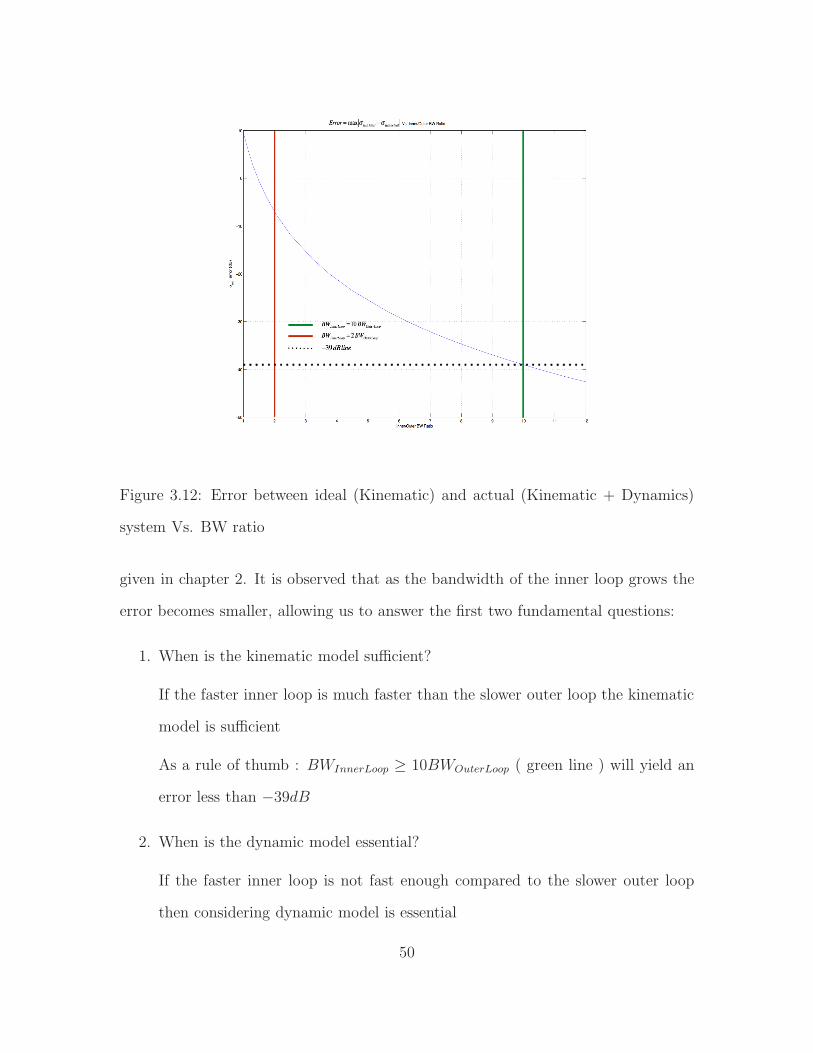
Figure 3.12: Error between ideal (Kinematic) and actual (Kinematic + Dynamics)

system Vs. BW ratio

given in chapter 2. It is observed that as the bandwidth of the inner loop grows the

error becomes smaller, allowing us to answer the first two fundamental questions:

1. When is the kinematic model sufficient?

If the faster inner loop is much faster than the slower outer loop the kinematic

model is sufficient

As a rule of thumb : BWInnerLoop ≥ 10BWOuterLoop ( green line ) will yield an

error less than −39dB

2. When is the dynamic model essential?

If the faster inner loop is not fast enough compared to the slower outer loop

then considering dynamic model is essential

50

As a rule of thumb: BWInnerLoop ≤ 2BWOuterLoop ( red line ) can yield and error

up to 10dB

3.3 Decentralized Control Limitation

From previous discussions we know that making the inner loop fast is desirable,

but of course operating at higher frequencies comes with a price, in our system this

price is the sensitivity function. Defining the sensitivity as

S = (I + PK)−1 =

S11 S12

S21 S22

(3.6)

It is critical for us that the peak of the elements of S are small in our frequency of

operation and also the off-diagonal element is much smaller that the diagonal element

so that the cross coupling is minimum.

(a) (b)

Figure 3.13: (a) max|S12| Vs. BW (b) max|S11| Vs. BW

Fig 3.13 plots the peak magnitude of these elements for systems with different

bandwidths, as bandwidth increases the peak becomes bigger which is undesirable.

51

10−3

10−2

10−1

100

101

102

103

104

−140

−120

−100

−80

−60

−40

−20

0

frequency (rad/sec)

|S12

/S11

|

Magnitude of Sensitivity Coupling (|S12/S11|) , varying BW

BW (σmin

) Incerasing

Figure 3.14: |S12

S11

|

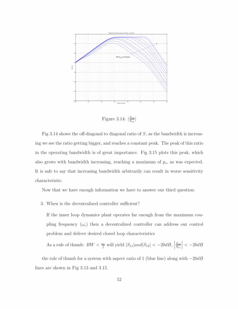
Fig 3.14 shows the off-diagonal to diagonal ratio of S, as the bandwidth is increas-

ing we see the ratio getting bigger, and reaches a constant peak. The peak of this ratio

in the operating bandwidth is of great importance. Fig 3.15 plots this peak, which

also grows with bandwidth increasing, reaching a maximum of ps, as was expected.

It is safe to say that increasing bandwidth arbitrarily can result in worse sensitivity

characteristic.

Now that we have enough information we have to answer our third question:

3. When is the decentralized controller sufficient?

If the inner loop dynamics plant operates far enough from the maximum cou-

pling frequency (ωc) then a decentralized controller can address our control

problem and deliver desired closed loop characteristics

As a rule of thumb: BW < ωc

fwill yield |S11|and|S12| < −20dB,

∣

∣

∣

S12

S11

∣

∣

∣< −20dB

the rule of thumb for a system with aspect ratio of 1 (blue line) along with −20dB

lines are shown in Fig 3.13 and 3.15.

52

RAR Changing

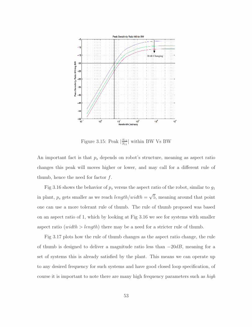
Figure 3.15: Peak |S12

S11| within BW Vs BW

An important fact is that ps depends on robot’s structure, meaning as aspect ratio

changes this peak will moves higher or lower, and may call for a different rule of

thumb, hence the need for factor f .

Fig 3.16 shows the behavior of ps versus the aspect ratio of the robot, similar to g1

in plant, ps gets smaller as we reach length/width =√5, meaning around that point

one can use a more tolerant rule of thumb. The rule of thumb proposed was based

on an aspect ratio of 1, which by looking at Fig 3.16 we see for systems with smaller

aspect ratio (width > length) there may be a need for a stricter rule of thumb.

Fig 3.17 plots how the rule of thumb changes as the aspect ratio change, the rule

of thumb is designed to deliver a magnitude ratio less than −20dB, meaning for a

set of systems this is already satisfied by the plant. This means we can operate up

to any desired frequency for such systems and have good closed loop specification, of

course it is important to note there are many high frequency parameters such as high

53

Sweet Spot

Vs. Robot AspectRatio

Figure 3.16: ps Vs. Aspect Ratio

0 0.5 1 1.5 2 2.5 3 3.5 4

5

10

15

20

25

30

35

40

Length/Width Ratio

f (ru

le o

f thu

mb

fact

or)

Rule of Thumb Ratio Vs. Robot Length/Width Ratio

Sweet Spot

Figure 3.17: Rule of thumb Vs. Aspect Ratio

frequency noise, sensor noise, saturation and non-linearties that are being neglected

here.

54

For boundary systems the rule of thumb is BW < ωc/4, this means operating

at any frequency above this point will not deliver desired specification unless we are

meeting the ideal aspect ratio range. This bring us to our last question:

4. When is the centralized controller essential?

If we operate close to the maximum coupling frequency (ωc) then a centralized

controller is essential

As an intuitive rule of thumb: BW > ωc

3.4 Centralized Control (Linear Quadratic Regulator)

This section is dedicated to design and analysis of a centralized controller for

mobile robot dynamics. Controller of choice is a Linear Quadratic Regulator with

full state feedback.

The plant is defined in Eq to Eq. In order to achieve zero steady state error to step

reference command two integrator have to be augmented to the plant output. The

augmented plant, denoted by Pd has the state equation:

x = Ax+Bu (3.7)

where

u = up (3.8)

x =

xI

xp

=

xI

yp

xr

(3.9)

xI = [θ1 θ2]T are the integrator states and xr is the rest of the plant’s states other

55

than plant outputs yp. Now by minimizing the quadratic cost function one can reach

a optimal control law for such plant:

J(u) =1

2

∫

∞

0

(xtQx+ ρutu)dt (3.10)

where ρ = 0.01 and Q = diag[1, 1, 1, 1, qIa1, qIa2, 2, 2]. qIa1 and qIa2 penalize the

armature currents allowing for different coupling characteristics as discussed further

in the following section. Selecting u = −Gx where G = [Gyp Gr GI ] will result in an

LQR architecture shown in Fig 3.18.

2-DC motors + Mobile Robot

Dynamics

yp =

[

ωR

ωL

]

+-

[

ωRref

ωLref

]

Xr =

Ia1

Ia2

ω

v

+-

Gr

Gyp

I

SGI

u

Figure 3.18: Dynamics Plant with a Linear Quadratic Regulator

As stated in section 3.3, the closed loop coupling ratio (∣

∣

∣

Tωωref12

Tωωref11

∣

∣

∣) has a constant

peak at high frequencies, which is dependent on the aspect ratio of the robot. Using

a decentralized controller, one can increase the closed loop peak frequency (ωC) by

increasing the bandwidth of the system ( Fig 3.19 ). While increasing the bandwidth

results in some desirable closed loop characteristics, as discussed in section 3.3 can

cause undesirable properties as well. On the other hand, using a centralized LQR

controller and a proper selection of Q, it is possible to shape the closed loop coupling

ratio.

56

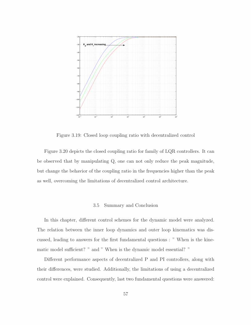
10−2

10−1

100

101

102

103

104

−120

−110

−100

−90

−80

−70

−60

−50

−40

−30

−20

Kp and K

i increasing

Figure 3.19: Closed loop coupling ratio with decentralized control

Figure 3.20 depicts the closed coupling ratio for family of LQR controllers. It can

be observed that by manipulating Q, one can not only reduce the peak magnitude,

but change the behavior of the coupling ratio in the frequencies higher than the peak

as well, overcoming the limitations of decentralized control architecture.

3.5 Summary and Conclusion

In this chapter, different control schemes for the dynamic model were analyzed.

The relation between the inner loop dynamics and outer loop kinematics was dis-

cussed, leading to answers for the first fundamental questions : ” When is the kine-

matic model sufficient? ” and ” When is the dynamic model essential? ”

Different performance aspects of decentralized P and PI controllers, along with

their differences, were studied. Additionally, the limitations of using a decentralized

control were explained. Consequently, last two fundamental questions were answered:

57

10−2

10−1

100

101

102

103

104

−90

−80

−70

−60

−50

−40

−30

−20

−10

0

Off−Diagonal to Diagonal ratio of Tω v, LQR Controller

frequency (rad/sec)

Mag

nitu

de (

dB)

Figure 3.20: Closed loop coupling ratio with centralized control

” When is the decentralized control sufficient? ” and ” When is the centralized control

essential?”

Finally, by implementing a centralized control architecture ( LQR ) and perform-

ing further analysis, it was possible to show that the centralized control is able to

overcome limitations of the decentralized scheme.

58

Chapter 4

TRAJECTORY PLANNING

4.1 Planning

In an industrial setting or in the field a mobile robot needs a trajectory to follow

and complete a goal. Planning this trajectory can be done in many different ways to

satisfy conditions such as minimum distance, minimum travel time, etc. However, in

general, this task can be broken down into finding a path and define a required timing

law on such path.

Trajectory planning is a considerably challenging topic. What can make this topic

even more challenging topic in non-holonomic systems is the fact that not only it has

to meet the boundary conditions. However, the non-holonomic constraint has to sat-

isfied at all points.

In this chapter path planning for a non-holonomic mobile robot and timing law

is discussed. A flat output system and its characteristics is then defined. Finally

admissible trajectory planning is thoroughly discussed.

4.2 Trajectory:Path and Timing law

Consider a trajectory q(t), t ∈ [ti, tf ] that guides a mobile robot from initial

configuration q(ti) = qi to final configuration q(tf ) = qt in time T = ti − tf . This

trajectory can be broken down into a geometric path q(g), where dq(g)dg

6= 0 and a

59

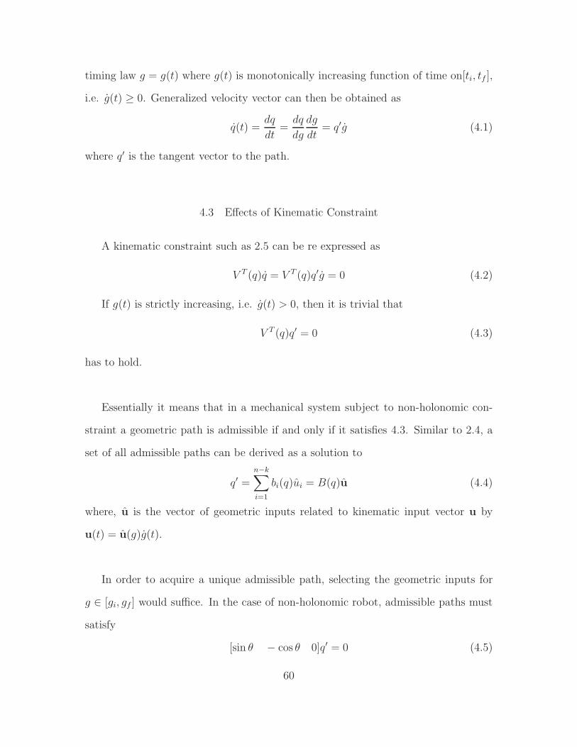
timing law g = g(t) where g(t) is monotonically increasing function of time on[ti, tf ],

i.e. g(t) ≥ 0. Generalized velocity vector can then be obtained as

q(t) =dq

dt=

dq

dg

dg

dt= q′g (4.1)

where q′ is the tangent vector to the path.

4.3 Effects of Kinematic Constraint

A kinematic constraint such as 2.5 can be re expressed as

V T (q)q = V T (q)q′g = 0 (4.2)

If g(t) is strictly increasing, i.e. g(t) > 0, then it is trivial that

V T (q)q′ = 0 (4.3)

has to hold.

Essentially it means that in a mechanical system subject to non-holonomic con-

straint a geometric path is admissible if and only if it satisfies 4.3. Similar to 2.4, a

set of all admissible paths can be derived as a solution to

q′ =

n−k∑

i=1

bi(q)ui = B(q)u (4.4)

where, u is the vector of geometric inputs related to kinematic input vector u by

u(t) = u(g)g(t).

In order to acquire a unique admissible path, selecting the geometric inputs for

g ∈ [gi, gf ] would suffice. In the case of non-holonomic robot, admissible paths must

satisfy

[sin θ − cos θ 0]q′ = 0 (4.5)

60

Therefore, all the admissible paths can be formulated as

x′

y′

θ′

=

cos θ 0

sin θ 0

0 1

v

ω

(4.6)

where,

v(t) = v(g)g(t) (4.7)

ω(t) = ω(g)g(t) (4.8)

The kinematic constraint in Equation 4.5 states that an admissible path for a

non-holonomic robot should have a tangent aligned with the robot’s sagittal axis. In

another words, no edges or sharp points are allowed on the path.

4.4 Differential Flatness

Consider a non-linear system defined by

x = f(x) + g(x)u (4.9)

y = h(x) + d(x)u (4.10)

Such system is differentially flat if there exists a set of outputs y, where states x

and control inputs u can be expressed as unique functions of y and its derivatives:

x = fcn1(y, y, y, ..., y(n)) (4.11)

u = fcn2(y, y, y, ..., y(n)) (4.12)

Outputs y are called flat outputs. Cartesian coordinates [x, y] in mobile robots

are considered flat outputs, consider geometric model in Equation 4.6, by defining an

output Cartesian path [x(g), y(g)] one can calculate the orientation from

θ(g) = atan2(y′(g), x′(g)) + kπ k = 0, 1 (4.13)

61

where, k defines if the robot is moving forward (k = 0) or backward (k = 1) and

atan2 is a variation of arctangent 1 that calculates the angle between the x axis and

the line passing through point (x, y) from origin.

The states are then obtained as q(g) = [x(g) y(g) θ(g)]T and the geometric

velocity inputs are uniquely defined by Equation 4.14 and 4.15.

v(g) = ±√

x′(g)2 + y′(g)2 (4.14)

ω(g) =y′′(g)x′(g)− x′′(g)y′(g)

x′(g)2 + y′(g)2(4.15)

This means that a unique path along with unique velocities can be defined for the

robot.

4.5 Conclusion

In this chapter the outer loop path generation problem of the mobile robot was

discussed. For this purpose, generating viable speed commands for a desired path

had more focus on.

At first, path planning for non-holonomic mobile robots were presented. After

defining a flat output system and the features incorporated with it, trajectory plan-

ning was fully explained.

1Using tangent half formula an expression can be derived : atan2 = 2arctan(y/(√

x2 + y2 + x))

62

Chapter 5

SUMMARY AND FUTURE WORK

In this thesis, a thorough discussion on mobile robot control & design, and the

problems and limitations incorporated with it, was provided. Additionally, commonly

neglected aspects of mobile robot design in the literature were explained. Four funda-

mental questions were proposed, were answers to them would clarify such neglected

aspects.

A thorough study of mobile robot kinematics and dynamics were performed, and

the design aspects of a differential drive mobile robot was discussed. The dependency

between shape, power and mass of the robot on dynamics and coupling was clearly

addressed. Based on such dependencies, facilitating a kinematic-only design through

desirable plant characteristics was studied.

Next the relation between the inner loop dynamics and the outer loop kinematics

was discussed, leading to answers to the first two fundamental questions proposed

earlier:

1. When is the kinematic model sufficient?

When ( Faster Inner ) Velocity Loop is much faster than ( Slower Outer )

Position Loop

2. When is the dynamic model essential?

When ( Faster Inner ) Velocity Loop is not fast enough compared to ( Slower

Outer ) Position Loop

63

The performance of decentralized control was then studied and the limitation of

such control structure was exposed in terms of the closed loop characteristics. Based

on such analysis answers were provided to the last two fundamental questions:

3. When is the decentralized control sufficient?

When system operates at low enough frequencies with respect to coupling peak

4. When is the centralized control essential?

When system operates at frequencies close to coupling peak or higher frequencies

Finally a centralized control architecture ( LQR Servo ) was implemented con-

firming the possibility of overcoming limitation arising from the centralized control.

In this thesis, many details concerning design and control of mobile robots were

discussed and addressed, however mobile robotic is a very vast and complicated field

of science, and one can always go into more details about every aspect of it. The

following topics are proposed as a guideline for possible future work for this article:

• More complicated inner loop dynamics

As discussed before there are parameters such as surface friction] and saturation

that yet to be considered in the dynamic plant, allowing further analysis for more

aggressive specification ( higher bandwidth, less cross coupling ) of such plant.

Additionally further analysis on the structured and unstructured uncertainties

( parametric/dynamic ) of the plant, and robustness of different control scheme

to such uncertainties is suggested.

• Outer loop kinematics issues

Position control aspect of mobile robot, such as outer loop control design and

performance analysis has yet to be discussed in greater details. A systematic

comparison of distinct combination of outer loop and inner loop strategies is

highly suggested.

64

• Hardware Implementation

The proposed material in this document has provided a guide to design and

control differential drive mobile robots, while minimizing undesirable charac-

teristics of such system. The next step is to design and implement a robot

based on results driven in this thesis. Of course an important discussion which

would be complementary to our results is the trade off analysis between desired

performance and cost for an actual system.

65

REFERENCES

[1] M.E. Rosheim. In the footsteps of leonardo [articulated anthropomorphic robot].Robotics Automation Magazine, IEEE, 4(2):12–14, 1997.

[2] RD Schraft and G Schmierer. Serviceroboter, 1998.

[3] Joseph L Jones and Anita M Flynn. Mobile robots: inspiration to implementa-tion. AK Peters, Ltd., 1993.

[4] Peter F Bladin. W. grey walter, pioneer in the electroencephalogram, robotics,cybernetics, artificial intelligence. Journal of clinical neuroscience, 13(2):170–177, 2006.

[5] P Marsh. Machines with mobilityjohns hopkins beast robot. Robots, 1985.

[6] S Lawrence Bellinger. Self-propelled random motion lawnmower, March 16 1971.US Patent 3,570,227.

[7] Joseph F Engelberger. Health-care robotics goes commercial: the helpmateex-perience. Robotica, 11(06):517–523, 1993.

[8] Claude Samson and K Ait-Abderrahim. Feedback control of a nonholonomicwheeled cart in cartesian space. In Robotics and Automation, 1991. Proceedings.,1991 IEEE International Conference on, pages 1136–1141. IEEE, 1991.

[9] Brigitte d’Andrea Novel, Gianni Campion, and Georges Bastin. Control of non-holonomic wheeled mobile robots by state feedback linearization. The Interna-tional journal of robotics research, 14(6):543–559, 1995.

[10] Alessandro De Luca and Marika D Di Benedetto. Control of nonholonomicsystems via dynamic compensation. Kybernetika, 29(6):593–608, 1993.

[11] G. Klancar, D. Matko, and S. Blazic. Mobile robot control on a reference path. InIntelligent Control, 2005. Proceedings of the 2005 IEEE International Symposiumon, Mediterrean Conference on Control and Automation, pages 1343–1348, 2005.

[12] Shouling He. Feedback control design of differential-drive wheeled mobile robots.In Advanced Robotics, 2005. ICAR’05. Proceedings., 12th International Confer-ence on, pages 135–140. IEEE, 2005.

[13] Bruno Siciliano, Lorenzo Sciavicco, Luigi Villani, and Giuseppe Oriolo. Robotics:modelling, planning and control. Springer, 2011.

[14] A Ollero and O Amidi. Predictive path tracking of mobile robots. applicationto the cmu navlab. In Proceedings of 5th International Conference on AdvancedRobotics, Robots in Unstructured Environments, ICAR, volume 91, pages 1081–1086, 1991.

66

[15] Julio E Normey-Rico, Juan Gomez-Ortega, and Eduardo F Camacho. A smith-predictor-based generalised predictive controller for mobile robot path-tracking.Control Engineering Practice, 7(6):729–740, 1999.

[16] Gregor Klancar and Igor Skrjanc. Tracking-error model-based predictive controlfor mobile robots in real time. Robotics and Autonomous Systems, 55(6):460–469,2007.

[17] Y. Kanayama, Y. Kimura, F. Miyazaki, and T. Noguchi. A stable trackingcontrol method for an autonomous mobile robot. In Robotics and Automation,1990. Proceedings., 1990 IEEE International Conference on, pages 384–389 vol.1,1990.

[18] Roland Siegwart and Illah Reza Nourbakhsh. Intro to Autonomous MobileRobots. MIT press, 2004.

[19] PK Padhy, Takeshi Sasaki, Sousuke Nakamura, and Hideki Hashimoto. Modelingand position control of mobile robot. In Advanced Motion Control, 2010 11thIEEE International Workshop on, pages 100–105. IEEE, 2010.

[20] Frederico C Vieira, Adelardo AD Medeiros, Pablo J Alsina, and Antonio PAraujo Jr. Position and orientation control of a two-wheeled differentially drivennonholonomic mobile robot. In ICINCO (2), pages 256–262, 2004.

[21] A.D. Araujo, P.J. Alsina, and S.M. Dias. Nonholonomic wheeled mobile robotpositioning controller using decoupling and variable structure model referenceadaptive control. In American Control Conference, 2006, pages 6 pp.–, 2006.

[22] Alessandro De Luca, Giuseppe Oriolo, and Marilena Vendittelli. Control ofwheeled mobile robots: An experimental overview. In Ramsete, pages 181–226.Springer, 2001.

[23] G. Oriolo, A. De Luca, and M. Vendittelli. Wmr control via dynamic feedbacklinearization: design, implementation, and experimental validation. Control Sys-tems Technology, IEEE Transactions on, 10(6):835–852, 2002.

[24] R. Fierro and F.L. Lewis. Control of a nonholonomic mobile robot: backsteppingkinematics into dynamics. In Decision and Control, 1995., Proceedings of the34th IEEE Conference on, volume 4, pages 3805–3810 vol.4, 1995.

[25] S. Nandy, S.N. Shome, G. Chakraborty, and C.S. Kumar. A modular approachto detailed dynamic formulation and control of wheeled mobile robot. In Mecha-tronics and Automation (ICMA), 2011 International Conference on, pages 1471–1478, 2011.

[26] Divya Aneesh. Tracking controller of mobile robot. In Computing, Electronicsand Electrical Technologies (ICCEET), 2012 International Conference on, pages343–349. IEEE, 2012.

67

[27] Francesco Mondada, Edoardo Franzi, and Andre Guignard. The development ofkhepera. In Proceedings of the 1st international Khepera workshop, volume 64,pages 7–13. Citeseer, 1999.

[28] Richard C Dorf and Robert H Bishop. Modern control systems. Pearson, 2011.

[29] Richard C Dorf and Robert H Bishop. Modern Control Systems: Solutions Man-ual. Addison-Wesley, 1998.

[30] Naresh K Sinha, Colin D Dicenzo, and Barna Szabados. Modeling of dc motorsfor control applications. Industrial Electronics and Control Instrumentation,IEEE Transactions on, (2):84–88, 1974.

[31] Gerald Cook. Mobile robots: navigation, control and remote sensing. Wiley-IEEEPress, 2011.

68

APPENDIX A

MATLAB CODES

69

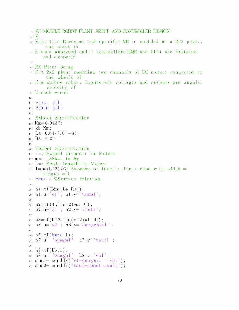
1 %% MOBILE ROBOT PLANT SETUP AND CONTROLLER DESIGN2 %3 % In th i s Document and s p e c i f i c MR i s modeled as a 2x2 plant ,

the p lant i s4 % then analyzed and 2 c o n t r o l l e r s (LQR and PID) are des igend

and compared5

6 %% Plant Setup7 % A 2x2 plant modeling two channe l s o f DC motors connected to

the wheels o f8 % a mobile robot , Inputs are vo l t a g e s and outputs are angular

v e l o c i t y o f9 % each wheel

10

11 c l e a r a l l ;12 c l o s e a l l ;13

14 %Motor S p e c i f i c a t i o n15 Km=0.0487;16 kb=Km;17 La=0.64∗(10ˆ−3) ;18 Ra=0.27 ;19

20 %Robot S p e c i f i c a t i o n21 r=; %wheel diameter in Meters22 m=; %Mass in Kg23 L=; %Axis l ength in Meters24 I=m∗(Lˆ2) /6 ; %moment o f i n e r t i a f o r a cube with width =

length = L25 beta=; %Sur face f r i c t i o n26

27 h1=t f (Km, [ La Ra ] ) ;28 h1 . u=’ e1 ’ ; h1 . y=’ taum1 ’ ;29

30 h2=t f ( 1 , [ ( r ˆ2)∗m 0 ] ) ;31 h2 . u=’ x1 ’ ; h2 . y=’ vhat1 ’ ;32

33 h3=t f (Lˆ2 , [ 2∗ ( r ˆ2)∗ I 0 ] ) ;34 h3 . u=’ x2 ’ ; h3 . y=’ omegahat1 ’ ;35

36 h7=t f ( beta , 1 ) ;37 h7 . u= ’ omega1 ’ ; h7 . y=’ tau f1 ’ ;38

39 h8=t f (kb , 1 ) ;40 h8 . u= ’ omega1 ’ ; h8 . y=’ vb1 ’ ;41 sum1= sumblk ( ’ e1=omegar1 − vb1 ’ ) ;42 sum2= sumblk ( ’ tau1=taum1−tau f1 ’ ) ;

70

43 sum3= sumblk ( ’ x1=tau1+tau2 ’ ) ;44 sum4= sumblk ( ’ x2=tau1−tau2 ’ ) ;45 sum5= sumblk ( ’ omega1 = vhat1 + omegahat1 ’ ) ;46

47

48 h4=t f (Km, [ La Ra ] ) ;49 h4 . u=’ e2 ’ ; h4 . y=’ taum2 ’ ;50

51 h6=t f ( 1 , [ ( r ˆ2)∗m 0 ] ) ;52 h6 . u=’ x4 ’ ; h6 . y=’ vhat2 ’ ;53

54 h5=t f (Lˆ2 , [ 2∗ ( r ˆ2)∗ I 0 ] ) ;55 h5 . u=’ x3 ’ ; h5 . y=’ omegahat2 ’ ;56

57 h9=t f ( beta , 1 ) ;58 h9 . u= ’ omega2 ’ ; h9 . y=’ tau f2 ’ ;59

60 h10=t f ( kb , 1 ) ;61 h10 . u= ’ omega2 ’ ; h10 . y=’ vb2 ’ ;62

63 sum6= sumblk ( ’ e2=omegar2 − vb2 ’ ) ;64 sum7= sumblk ( ’ tau2=taum2−tau f2 ’ ) ;65 sum8= sumblk ( ’ x3=tau1 − tau2 ’ ) ;66 sum9= sumblk ( ’ x4=tau2 + tau1 ’ ) ;67 sum10= sumblk ( ’ omega2 = vhat2 − omegahat2 ’ ) ;68

69 ML=connect ( s s ( h1 ) , h2 , h3 , s s ( h4 ) , h5 , h6 , h7 , h8 , h9 , h10 , sum1 , sum2 ,sum3 , sum4 , sum5 , sum6 , sum7 , sum8 , sum9 , sum10 ,{ ’ omegar1 ’ , ’omegar2 ’ } ,{ ’ omega1 ’ , ’ omega2 ’ }) ;

70 ML. statename={ ’ i a 1 ’ , ’ x2 ’ , ’ x3 ’ , ’ i a 2 ’ , ’ x5 ’ , ’ x6 ’ } ;71

72 %Plant Plot s73

74 %StepPlot75 f 1=f i g u r e ;76 f 1=s t epp l o t (ML) ;77 g r id on ;78 t i t l e ( ’ Step response o f the 2 Motor channels , Robot ’ ’ s

dynamics inc luded ’ ) ;79

80 %Singu la r Value p lo t81 f 2=f i g u r e ;82 f 2=sigmaplot (ML,{10ˆ−2 ,10ˆ4}) ;83 s e t op t i on s ( f2 , ’ FreqUnits ’ , ’Hz ’ ) ;84 g r id ;85 t i t l e ( ’ S ingu la r Values o f the p lant ’ ) ;86

71

87 MLmin=minrea l (ML, [ ] , 0 ) ;88 MLmin. u={ ’ omegar1n ’ , ’ omegar2n ’ } ;89 MLmin. y={ ’ omega1n ’ , ’ omega2n ’ } ;90

91 % StepPlot92 f 3=f i g u r e ;93 f 3=s t epp l o t (MLmin) ;94 g r id on ;95 t i t l e ( ’ Step response o f the 2 Motor channels , Robot ’ ’ s

dynamics inc luded ’ ) ;96

97 % ∗ S ingu la r Value p lo t98 f 4=f i g u r e ;99 f 4=sigmaplot (MLmin) ;

100 s e t op t i on s ( f4 , ’ FreqUnits ’ , ’Hz ’ ) ;101 g r id ;102 t i t l e ( ’ S ingu la r Values o f the 2 Motor channels , Robot ’ ’ s

dynamics inc luded ’ ) ;103

104 [ Aol , Bol , Col , Dol ]= ssdata (MLmin) ;105

106

107 k f f 1=1/dcgain (MLmin(1 , 1 ) ) ;108 k f f 2=1/dcgain (MLmin(2 , 2 ) ) ;109

110 FFrob=MLmin∗ [ k f f 1 , 0 ; 0 , k f f 2 ] ;111

112 FFrob . u={ ’ omegar1n ’ , ’ omegar2n ’ } ;113 FFrob . y={ ’ omega1n ’ , ’ omega2n ’ } ;114

115 % %StepPlot116 f f 1=f i g u r e ;117 f f 1=s t epp l o t (FFrob ) ;118 g r id on ;119 t i t l e ( ’ Step response o f the 2 Motor channe l s Feed Forward

Open Loop , Robot ’ ’ s dynamics inc luded ’ ) ;120

121 % %Singu la r Value p lo t122 f f 2=f i g u r e ;123 f f 2=sigmaplot (FFrob ) ;124 s e t op t i on s ( f f 2 , ’ FreqUnits ’ , ’Hz ’ ) ;125 g r id ;126 t i t l e ( ’ S ingu la r Values o f the 2 Motor channe l s Feed Forward

Open Loop , Robot ’ ’ s dynamics inc luded ’ ) ;127

128 %% LQR Design

72

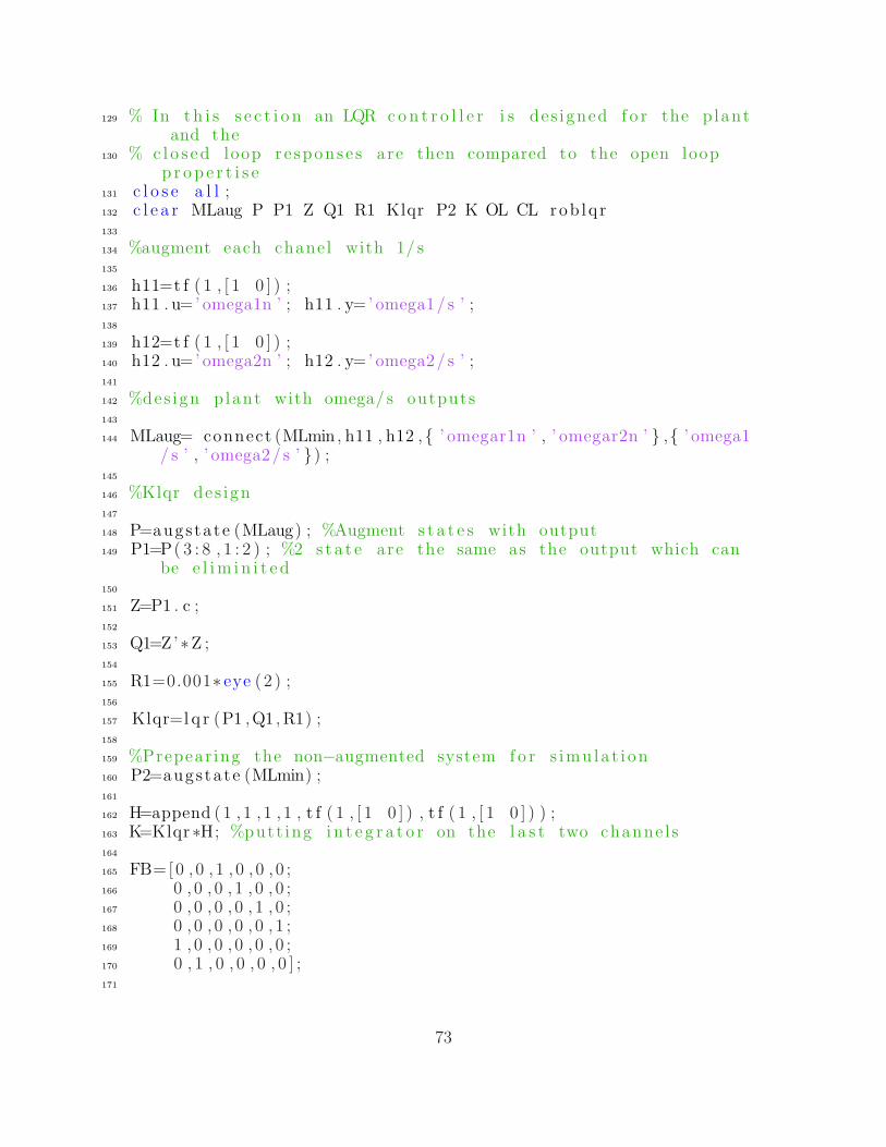
129 % In th i s s e c t i o n an LQR co n t r o l l e r i s des igned f o r the p lantand the

130 % c lo s ed loop r e sponse s are then compared to the open loopp r o p e r t i s e

131 c l o s e a l l ;132 c l e a r MLaug P P1 Z Q1 R1 Klqr P2 K OL CL rob lq r133

134 %augment each chanel with 1/ s135

136 h11=t f ( 1 , [ 1 0 ] ) ;137 h11 . u=’ omega1n ’ ; h11 . y=’ omega1/ s ’ ;138

139 h12=t f ( 1 , [ 1 0 ] ) ;140 h12 . u=’ omega2n ’ ; h12 . y=’ omega2/ s ’ ;141

142 %des ign p lant with omega/ s outputs143

144 MLaug= connect (MLmin , h11 , h12 ,{ ’ omegar1n ’ , ’ omegar2n ’ } ,{ ’ omega1/ s ’ , ’ omega2/ s ’ }) ;

145

146 %Klqr des ign147

148 P=augstate (MLaug) ; %Augment s t a t e s with output149 P1=P( 3 : 8 , 1 : 2 ) ; %2 s t a t e are the same as the output which can

be e l im i n i t e d150

151 Z=P1 . c ;152

153 Q1=Z’∗Z ;154

155 R1=0.001∗ eye (2 ) ;156

157 Klqr=l q r (P1 ,Q1 ,R1) ;158

159 %Prepear ing the non−augmented system f o r s imu la t i on160 P2=augstate (MLmin) ;161

162 H=append (1 , 1 , 1 , 1 , t f ( 1 , [ 1 0 ] ) , t f ( 1 , [ 1 0 ] ) ) ;163 K=Klqr∗H; %putt ing i n t e g r a t o r on the l a s t two channe l s164

165 FB=[0 , 0 , 1 , 0 , 0 , 0 ;166 0 , 0 , 0 , 1 , 0 , 0 ;167 0 , 0 , 0 , 0 , 1 , 0 ;168 0 , 0 , 0 , 0 , 0 , 1 ;169 1 , 0 , 0 , 0 , 0 , 0 ;170 0 , 1 , 0 , 0 , 0 , 0 ] ;171

73

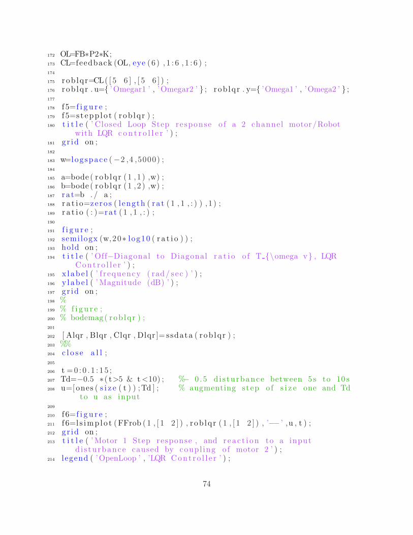
172 OL=FB∗P2∗K;173 CL=feedback (OL, eye (6 ) , 1 : 6 , 1 : 6 ) ;174

175 r ob lq r=CL( [ 5 6 ] , [ 5 6 ] ) ;176 r ob lq r . u={ ’Omegar1 ’ , ’Omegar2 ’ } ; r ob lq r . y={ ’Omega1 ’ , ’Omega2 ’ } ;177

178 f 5=f i g u r e ;179 f 5=s t epp l o t ( r ob lq r ) ;180 t i t l e ( ’ Closed Loop Step response o f a 2 channel motor/Robot

with LQR co n t r o l l e r ’ ) ;181 g r id on ;182

183 w=log space (−2 ,4 ,5000) ;184

185 a=bode ( rob lq r (1 , 1 ) ,w) ;186 b=bode ( rob lq r (1 , 2 ) ,w) ;187 r a t=b . / a ;188 r a t i o=zero s ( l ength ( ra t ( 1 , 1 , : ) ) ,1 ) ;189 r a t i o ( : )=ra t ( 1 , 1 , : ) ;190

191 f i g u r e ;192 semi logx (w,20∗ l og10 ( r a t i o ) ) ;193 hold on ;194 t i t l e ( ’ Off−Diagonal to Diagonal r a t i o o f T {\omega v} , LQR

Cont r o l l e r ’ ) ;195 x l ab e l ( ’ f r equency ( rad/ sec ) ’ ) ;196 y l ab e l ( ’Magnitude (dB) ’ ) ;197 g r id on ;198 %199 % f i g u r e ;200 % bodemag( rob lq r ) ;201

202 [ Alqr , Blqr , Clqr , Dlqr ]= ssdata ( rob lq r ) ;203 %%204 c l o s e a l l ;205

206 t =0 : 0 . 1 : 1 5 ;207 Td=−0.5 ∗( t>5 & t<10) ; %− 0 . 5 d i s tu rbance between 5 s to 10 s208 u=[ones ( s i z e ( t ) ) ;Td ] ; % augmenting step o f s i z e one and Td

to u as input209

210 f 6=f i g u r e ;211 f 6=l s imp l o t (FFrob ( 1 , [ 1 2 ] ) , r ob lq r ( 1 , [ 1 2 ] ) , ’−− ’ ,u , t ) ;212 g r id on ;213 t i t l e ( ’Motor 1 Step response , and r ea c t i on to a input

d i s tu rbance caused by coupl ing o f motor 2 ’ ) ;214 l egend ( ’OpenLoop ’ , ’LQR Cont r o l l e r ’ ) ;

74

215

216 u1=[Td ; ones ( s i z e ( t ) ) ] ;217 f 7=f i g u r e ;218 f 7=l s imp l o t (FFrob ( 2 , [ 1 2 ] ) , r ob lq r ( 2 , [ 1 2 ] ) , ’−− ’ , u1 , t ) ;219 g r id on ;220 t i t l e ( ’Motor 2 Step response , and r ea c t i on to a input

d i s tu rbance caused by coupl ing o f motor 1 ’ ) ;221 l egend ( ’OpenLoop ’ , ’LQR Cont r o l l e r ’ ) ;222 %ML aug= connect (ML, h11 , h12 ,{ ’ omegar1 ’ , ’ omegar2 ’} ,{ ’ omega1 ’ , ’

omega1/s ’ , ’ omega2 ’ , ’ omega2/s ’ } ) ;223

224 f 8=f i g u r e ;225 f 8=s t epp l o t (FFrob , rob lqr , ’−− ’ ) ;226 g r id on ;227 t i t l e ( ’ s t ep response o f the Openloop VS Closed Loop ’ ) ;228 l egend ( ’Open Loop ’ , ’LQR Cont r o l l e r ’ ) ;229

230 f 9=f i g u r e ;231 f 9=sigmaplot (FFrob ) ;232 hold on ;233 s igmaplot ( rob lqr , ’−− ’ ) ;234 g r id on ;235 l egend ( ’Open Loop ’ , ’LQR Cont r o l l e r ’ ) ;236

237 f 10=f i g u r e ;238 f 10=l s imp l o t ( rob lqr , u , t ) ;239 g r id on ;240 t i t l e ( ’Motor 1 Step response , and r ea c t i on to a input

d i s tu rbance caused by coupl ing o f motor 2 ’ ) ;241 l egend ( ’LQR Cont r o l l e r ’ ) ;242

243

244 f 11=f i g u r e ;245 f 11=l s imp l o t ( rob lqr , u1 , t ) ;246 g r id on ;247 t i t l e ( ’Motor 2 Step response , and r ea c t i on to a input

d i s tu rbance caused by coupl ing o f motor 1 ’ ) ;248 l egend ( ’LQR Cont r o l l e r ’ ) ;249

250 %% PI Cont r o l l e r251 % In th i s s e c t i o n a PI c o n t r o l l e r i s des igend f o r each

channel252

253 C1=pidtune (MLmin(1 , 1 ) , ’ p i ’ ) ;254 C2=pidtune (MLmin(2 , 2 ) , ’ p i ’ ) ;255 % C1 . k i =1;256 % C2 . k i =1;

75

257 C1 . kp=10;258 C2 . kp=10;259 KPID=append (C1 ,C2) ;260

261 FF=MLmin∗KPID ;262

263 robpid=feedback (FF, eye (2 ) ) ;264

265 w=log space (−2 ,4 ,100) ;266

267 a=bode ( robpid (1 , 1 ) ,w) ;268 b=bode ( robpid (1 , 2 ) ,w) ;269 r a t=b . / a ;270 r a t i o=zero s ( l ength ( ra t ( 1 , 1 , : ) ) ,1 ) ;271 r a t i o ( : )=ra t ( 1 , 1 , : ) ;272

273 semi logx (w,20∗ l og10 ( r a t i o ) , ’ k−− ’ ) ;274

275 % st epp l o t ( robpid ) ;276 %% PID vs . LQR277 % The f o l l ow ing p l o t s prov ide a comparison between PI and LQR

c o n t r o l l e r s278 % fo r the same plant279

280 c l o s e a l l ;281

282 t =0 : 0 . 1 : 1 5 ;283 Td=−0.5 ∗( t>5 & t<10) ; %− 0 . 5 d i s tu rbance between 5 s to 10 s284 u=[ones ( s i z e ( t ) ) ;Td ] ; % augmenting step o f s i z e one and Td

to u as input285

286 f 6=f i g u r e ;287 f 6=l s imp l o t ( robpid ( 1 , [ 1 2 ] ) , r ob lq r ( 1 , [ 1 2 ] ) , ’−− ’ ,u , t ) ;288 g r id on ;289 t i t l e ( ’Motor 1 Step response , and r ea c t i on to a input

d i s tu rbance caused by coupl ing o f motor 2 ’ ) ;290 l egend ( ’PID Cont r o l l e r ’ , ’LQR Cont r o l l e r ’ ) ;291

292 u1=[Td ; ones ( s i z e ( t ) ) ] ;293 f 7=f i g u r e ;294 f 7=l s imp l o t ( robpid ( 2 , [ 1 2 ] ) , r ob lq r ( 2 , [ 1 2 ] ) , ’−− ’ , u1 , t ) ;295 g r id on ;296 t i t l e ( ’Motor 2 Step response , and r ea c t i on to a input

d i s tu rbance caused by coupl ing o f motor 1 ’ ) ;297 l egend ( ’PID Cont r o l l e r ’ , ’LQR Cont r o l l e r ’ ) ;298 %ML aug= connect (ML, h11 , h12 ,{ ’ omegar1 ’ , ’ omegar2 ’} ,{ ’ omega1 ’ , ’

omega1/s ’ , ’ omega2 ’ , ’ omega2/s ’ } ) ;

76

299

300 f 8=f i g u r e ;301 f 8=s t epp l o t ( robpid , rob lqr , ’−− ’ ) ;302 g r id on ;303 t i t l e ( ’ s t ep response o f the Openloop VS Closed Loop ’ ) ;304 l egend ( ’PID Cont r o l l e r ’ , ’LQR Cont r o l l e r ’ ) ;305

306 f 9=f i g u r e ;307 f 9=sigmaplot ( robpid ) ;308 hold on ;309 s igmaplot ( rob lqr , ’−− ’ ) ;310 g r id on ;311 l egend ( ’PID Cont r o l l e r ’ , ’LQR Cont r o l l e r ’ ) ;312

313 f 10=f i g u r e ;314 f 10=l s imp l o t ( rob lqr , u , t ) ;315 g r id on ;316 t i t l e ( ’Motor 1 Step response , and r ea c t i on to a input

d i s tu rbance caused by coupl ing o f motor 2 ’ ) ;317 l egend ( ’LQR Cont r o l l e r ’ ) ;318

319

320 f 11=f i g u r e ;321 f 11=l s imp l o t ( rob lqr , u1 , t ) ;322 g r id on ;323 t i t l e ( ’Motor 2 Step response , and r ea c t i on to a input

d i s tu rbance caused by coupl ing o f motor 1 ’ ) ;324 l egend ( ’LQR Cont r o l l e r ’ ) ;325

326 f 10=f i g u r e ;327 f 10=l s imp l o t ( robpid , u , t ) ;328 g r id on ;329 t i t l e ( ’Motor 1 Step response , and r ea c t i on to a input

d i s tu rbance caused by coupl ing o f motor 2 ’ ) ;330 l egend ( ’PID Cont r o l l e r ’ ) ;331

332

333 f 11=f i g u r e ;334 f 11=l s imp l o t ( robpid , u1 , t ) ;335 g r id on ;336 t i t l e ( ’Motor 2 Step response , and r ea c t i on to a input

d i s tu rbance caused by coupl ing o f motor 1 ’ ) ;337 l egend ( ’PID Cont r o l l e r ’ ) ;338

339

340 %% Sen s i t i v i t y a n a l y s i s

77

341 % This s e c t i o n S en s e t i v i t y and Complement s e n s i t i v i t y o ffo rmer ly des igned

342 % c o n t r o l l e r s are p l o t t ed and compared343

344 c l o s e a l l ;345

346 Plant=FB∗P2 ;347 Cont r o l l e r=ss (K) ;348 Loopslqr=loopsens ( Plant , Con t r o l l e r ) ;349

350 Loopspid=loopsens (MLmin,KPID) ;351

352 f i g u r e ;353 bodemag( Loopslqr . Si , Loopspid . S i ) ;354 t i t l e ( ’ S e n s i t i v i t y Bode Magnitude ’ ) ;355 l egend ( ’LQR Cont r o l l e r ’ , ’PID Cont r o l l e r s ’ ) ;356 g r id on ;357

358 f i g u r e ;359 f 19=bodeplot ( Loopslqr . Si , Loopspid . S i ) ;360 t i t l e ( ’ S e n s i t i v i t y Bode Phase ’ ) ;361 l egend ( ’LQR Cont r o l l e r ’ , ’PID Cont r o l l e r s ’ ) ;362 g r id on ;363 s e t op t i on s ( f19 , ’ MagVisible ’ , ’ o f f ’ ) ;364

365

366 f i g u r e ;367 bodemag( Loopslqr . Ti , Loopspid . Ti ) ;368 t i t l e ( ’Complement S e n s i t i v i t y Bode Magnitude ’ ) ;369 l egend ( ’LQR Cont r o l l e r ’ , ’PID Cont r o l l e r ’ ) ;370 g r id on ;371

372 f i g u r e ;373 f 20=bodeplot ( Loopslqr . Ti , Loopspid . Ti ) ;374 t i t l e ( ’Complement S e n s i t i v i t y Bode Phase ’ ) ;375 l egend ( ’LQR Cont r o l l e r ’ , ’PID Cont r o l l e r s ’ ) ;376 g r id on ;377 s e t op t i on s ( f20 , ’ MagVisible ’ , ’ o f f ’ ) ;378

379 f i g u r e ;380 f 22=bodeplot ( Loopslqr . Si , Loopspid . S i ) ;381 t i t l e ( ’ S e n s i t i v i t y Bode ’ ) ;382 l egend ( ’LQR Cont r o l l e r ’ , ’PID Cont r o l l e r s ’ ) ;383 g r id on ;384

385 f i g u r e ;386 f 21=bodeplot ( Loopslqr . Ti , Loopspid . Ti ) ;

78

387 t i t l e ( ’Complement S e n s i t i v i t y Bode ’ ) ;388 l egend ( ’LQR Cont r o l l e r ’ , ’PID Cont r o l l e r s ’ ) ;389 g r id on ;

1 %%2 c l e a r a l l ;3 c l o s e a l l ;4 f 1=f i g u r e ;5

6 tmc= %motor torque constant ;7

8 f o r i =1: l ength ( tmc )9

10 %motor specs11 Km=tmc( i ) ;12 kb=;13 La=;14 Ra=;15 beta=;16 J=;17

18

19 h1= t f (Km, [ La ,Ra ] ) ;20 h1 . u=’ e ’ ; h1 . y= ’ tau ’ ;21

22 h2= t f ( 1 , [ J , beta ] ) ;23 h2 . u=’ tau ’ ; h2 . y= ’ omega ’ ;24

25 h3= t f ( kb , 1 ) ;26 h3 . u=’ omega ’ ; h3 . y=’ vb ’ ;27

28 sum1=sumblk ( ’ e=v−vb ’ ) ;29

30 dcm=connect ( s s ( h1 ) , h2 , h3 , sum1 , ’ v ’ ,{ ’ tau ’ , ’ omega ’ }) ;31

32 %33 t =0 :1 : 24 ;34 u=t ;35 [ y , t ]= l s im (dcm , u , t ) ;36 %37 Power ( i )=y (24 , 1 ) ∗y (24 , 2 ) ;38 Power2 ( i ) =(24ˆ2)∗beta ∗ ( (Km/( beta∗Ra+Km∗kb ) ) ˆ2) ; %Power in

watts39 Power ( i )=Power2 ( i ) ∗(1.341∗10ˆ−3) ; %Power in hp40 dc=Km/( beta∗Ra+Km∗kb ) ;41

42 end43

79

44 p lo t ( tmc , Power ) ;45 hold on ;46

47 p lo t ( tmc , Power , ’ r ’ ) ;48

49 %%50 c l e a r a l l ;51 c l o s e a l l ;52 f 1=f i g u r e ;53

54 R=%armature r e s i s t a n c e ;55

56 f o r i =1: l ength (R)57

58 Km=;59 kb=;60 La=;61 Ra=R( i ) ;62 beta=;63 J=;64

65

66 h1= t f (Km, [ La ,Ra ] ) ;67 h1 . u=’ e ’ ; h1 . y= ’ tau ’ ;68

69 h2= t f ( 1 , [ J , beta ] ) ;70 h2 . u=’ tau ’ ; h2 . y= ’ omega ’ ;71

72 h3= t f ( kb , 1 ) ;73 h3 . u=’ omega ’ ; h3 . y=’ vb ’ ;74

75 sum1=sumblk ( ’ e=v−vb ’ ) ;76

77 dcm=connect ( s s ( h1 ) , h2 , h3 , sum1 , ’ v ’ ,{ ’ tau ’ , ’ omega ’ }) ;78

79

80 Power2 ( i ) =(24ˆ2)∗beta ∗ ( (Km/( beta∗Ra+Km∗kb ) ) ˆ2) ; %Power inwatts

81 Power ( i )=Power2 ( i ) ∗(1.341∗10ˆ−3) ; %Power in hp82

83 end84 %85 % plo t ( tmc , Power ) ;86 % hold on ;87

88 p lo t (R, Power , ’ r ’ ) ;89

80

90

91 %% DC motor bandwidth req92

93 c l e a r a l l ;94 c l o s e a l l ;95 f 1=f i g u r e ;96

97 l i n e o r d e r={ ’b ’ , ’ g ’ , ’ r ’ , ’ c ’ , ’m’ , ’ k−. ’ , ’b−− ’ , ’ r−− ’ , ’ k−− ’ , ’b−. ’ ,’ r−. ’ , ’ g−− ’ } ;

98

99 tmc=[0 .01 0 .05 0 .08 0 . 1 0 . 3 0 . 4 0 . 6 0 . 7 0 . 9 2 3 4 ] ;100

101 f 2=f i g u r e ;102 f 3=f i g u r e ;103 f 4=f i g u r e ;104 f 5=f i g u r e ;105

106 f o r i =1: l ength ( tmc )107

108 Km=tmc( i ) ;109 kb=0.0847;110 La=0.64∗(10ˆ−3) ;111 Ra=0.27 ;112 beta =0.021 ;113 J=0.00057892;114

115

116 h1= t f (Km, [ La ,Ra ] ) ;117 h1 . u=’ e ’ ; h1 . y= ’ tau ’ ;118

119 h2= t f ( 1 , [ J , beta ] ) ;120 h2 . u=’ tau ’ ; h2 . y= ’ omega ’ ;121

122 h3= t f ( kb , 1 ) ;123 h3 . u=’ omega ’ ; h3 . y=’ vb ’ ;124

125 sum1=sumblk ( ’ e=v−vb ’ ) ;126

127 dcm=connect ( s s ( h1 ) , h2 , h3 , sum1 , ’ v ’ ,{ ’ tau ’ , ’ omega ’ }) ;128 f i g u r e ( f 1 ) ;129 s t epp l o t (dcm , l i n e o r d e r { i }) ;130 hold on ;131

132 f i g u r e ( f 2 ) ;133 bodemag(dcm , l i n e o r d e r { i }) ;134 hold on ;135 g r id on ;

81

136

137 bw( i )=bandwidth (dcm(2 ,1 ) ) ;138

139 Power2 ( i ) =(24ˆ2)∗beta ∗ ( (Km/( beta∗Ra+Km∗kb ) ) ˆ2) ; %Power inwatts

140 Power ( i )=Power2 ( i ) ∗(1.341∗10ˆ−3) ; %Power in hp141 % dc=Km/( beta∗Ra+Km∗kb ) ;142

143 f i g u r e ( f 4 ) ;144 pzmap(dcm , l i n e o r d e r { i }) ;145 hold on ;146

147 S=s t ep i n f o (dcm) ;148 s e t t ime ( i )=S (2 ) . Set t l ingTime ;149

150

151 end152 %153 % plo t ( tmc , Power ) ;154 % hold on ;155

156 % plo t ( tmc , Power , ’ r ’ ) ;157 f i g u r e ( f 3 ) ;158 p lo t (Power ,bw) ;159 g r id on ;160 x l ab e l ( ’Power ’ ) ;161 y l ab e l ( ’ Bandwidth ’ ) ;162

163 f i g u r e ( f 5 ) ;164 p lo t ( tmc , s e t t ime ) ;165

166 %% DC motor + va r i ab l e i n e r t i a p l o t s167

168 c l e a r a l l ;169 c l o s e a l l ;170 f 1=f i g u r e ;171

172 l i n e o r d e r={ ’b ’ , ’ g ’ , ’ r ’ , ’ c ’ , ’m’ , ’ k−. ’ , ’b−− ’ , ’ r−− ’ , ’ k−− ’ , ’b−. ’ ,’ r−. ’ , ’ g−− ’ } ;

173

174 tmc=[0 .01 0 .02 0 .04 0 .06 0 .0847 0 . 1 0 . 3 0 . 5 0 . 7 0 . 9 1 2 3 4 56 ] ;

175 i n e r t i a =(10ˆ−5) ∗ [ 10 40 60 70 80 9 0 ] ;176

177 f 2=f i g u r e ;178 f 3=f i g u r e ;179 f 4=f i g u r e ;

82

180 f o r j =1: l ength ( i n e r t i a )181

182 f o r i =1: l ength ( tmc )183

184 Km=tmc( i ) ;185 kb=0.0847;186 La=0.64∗(10ˆ−3) ;187 Ra=0.27 ;188 beta =0.021 ;189 J=i n e r t i a ( j ) ;190

191

192 h1= t f (Km, [ La ,Ra ] ) ;193 h1 . u=’ e ’ ; h1 . y=’ tau ’ ;194

195 h2= t f ( 1 , [ J , beta ] ) ;196 h2 . u=’ tau ’ ; h2 . y=’ omega ’ ;197

198 h3= t f ( kb , 1 ) ;199 h3 . u=’ omega ’ ; h3 . y=’ vb ’ ;200

201 sum1=sumblk ( ’ e=v−vb ’ ) ;202

203 dcm=connect ( s s ( h1 ) , h2 , h3 , sum1 , ’ v ’ ,{ ’ tau ’ , ’ omega ’ }) ;204

205 % f i g u r e ( f 2 ) ;206 % bodemag(dcm , l i n e o r d e r { i }) ;207 % hold on ;208 % gr id on ;209 %210 bw( j , i )=bandwidth (dcm(2 ,1 ) ) ;211

212 Power2 ( j , i ) =(24ˆ2)∗beta ∗ ( (Km/( beta∗Ra+Km∗kb ) ) ˆ2) ; %Power in watts

213 Power ( j , i )=Power2 ( i ) ∗(1.341∗10ˆ−3) ; %Power in hp214

215 end216 f i g u r e ( f 2 ) ;217 p lo t ( Power2 ( j , : ) ,bw( j , : ) , l i n e o r d e r { j }) ;218 hold on ;219 g r id on ;220

221 end222

223 %224 % plo t ( tmc , Power ) ;225 % hold on ;

83

226

227 % plo t ( tmc , Power , ’ r ’ ) ;228 % f i g u r e ( f 3 ) ;229 % plo t (Power ,bw) ;230 % gr id on ;231 % xlabe l ( ’ Power ’ ) ;232 % ylabe l ( ’ Bandwidth ’ ) ;233 %% PURE TF ana l y s i s o f the motor234 %235 c l e a r a l l ;236 c l o s e a l l ;237 f 1=f i g u r e ;238

239 % fo r k=1:40240

241 tmc=;242 f o r i =1: l ength ( tmc )243

244 Km=tmc( i ) ;245

246 kb=;247 La=;248 Ra=;249 beta=;250 J=;251

252 dcm=t f (Km, [ J∗La J∗Ra+beta∗La beta ∗Ra+Km∗kb ] ) ;253

254 f i g u r e ( f 1 ) ;255 pzmap(dcm) ;256 hold on ;257

258 dcg ( i )=dcgain (dcm) ;259 end260

261 %% PURE TF ana l y s i s o f the motor262 %263 c l e a r a l l ;264 c l o s e a l l ;265

266 l i n e o r d e r={ ’b ’ , ’ g ’ , ’ r ’ , ’ c ’ , ’m’ , ’ k−. ’ , ’b−− ’ , ’ r−− ’ , ’ k−− ’ , ’b−. ’ ,’ r−. ’ , ’ g−− ’ } ;

267 tmc=%motor torque constant ;268

269 f 1=f i g u r e ;270 f 2=f i g u r e ;271 f 3=f i g u r e ;

84

272 f 4=f i g u r e ;273 f 5=f i g u r e ;274

275 % fo r k=1:40276

277

278 f o r i =1: l ength ( tmc )279

280 Km=tmc( i ) ;281 kb=0.0847;282 La=0.64∗(10ˆ−3) ;283 Ra=0.27 ;284 beta =0.021 ;285 J=0.00057892;286

287 dcm=t f (Km, [ J∗La J∗Ra+beta∗La beta ∗Ra+Km∗kb ] ) ;288 %289 f i g u r e ( f 1 ) ;290 pzmap(dcm) ;291 hold on ;292 %293 f i g u r e ( f 2 ) ;294 bodemag(dcm , l i n e o r d e r { i }) ;295 hold on ;296 %297 f i g u r e ( f 3 ) ;298 s tep (dcm , l i n e o r d e r { i }) ;299 hold on ;300 %301 S=s t ep i n f o (dcm) ;302 s e t t ime ( i )=S . Set t l ingTime ;303

304 % bw( i )=bandwidth (dcm) ;305

306 vin=; %input vo l t age307 Ts=(Km/Ra) ∗vin ; %S t a l l Torque308 omega0=vin /kb ; %No load speed309 powermax( i )=(Ts∗omega0 ) /4 ;310 end311

312 f i g u r e ( f 4 ) ;313 p lo t ( tmc , powermax) ;314

315 f i g u r e ( f 5 ) ;316 p lo t ( tmc , s e t t ime ) ;317

318

85

319 hold on ;320

321 %% 2 dc motors comparison322 c l o s e a l l ;323 c l e a r a l l ;324

325

326 l i n e o r d e r={ ’b ’ , ’ g ’ , ’ r ’ , ’ c ’ , ’m’ , ’ k−. ’ , ’b−− ’ , ’ r−− ’ , ’ k−− ’ , ’b−. ’ ,’ r−. ’ , ’ g−− ’ } ;

327 tmc=[1000 2000 3000 4000 5000 6000 7000 8000 9000 10000 1100012000 ] ;

328

329 f 1=f i g u r e ;330 f 2=f i g u r e ;331 f 3=f i g u r e ;332 f 4=f i g u r e ;333 f 5=f i g u r e ;334

335 % fo r k=1:40336

337

338 f o r i =1: l ength ( tmc )339

340 Km2=tmc ( i ) ;341 kb2=;342 La2=;343 Ra2=;344 beta2=;345 J2=;346

347

348 dcm=t f (Km2, [ J2∗La2 J2∗Ra2+beta2∗La2 beta2∗Ra2+Km2∗kb2 ] ) ;349 %350 f i g u r e ( f 1 ) ;351 pzmap(dcm) ;352 hold on ;353 %354 f i g u r e ( f 2 ) ;355 bodemag(dcm , l i n e o r d e r { i }) ;356 hold on ;357 %358 f i g u r e ( f 3 ) ;359 s tep (dcm , l i n e o r d e r { i }) ;360 hold on ;361 %362 S=s t ep i n f o (dcm) ;363 s e t t ime ( i )=S . Set t l ingTime ;

86

364

365 % bw( i )=bandwidth (dcm) ;366

367 vin=24; %input vo l t age368 Ts=(Km2/Ra2) ∗( vin ˆ2) ; %S t a l l Torque369 omega0=vin /kb2 ; %No load speed370 powermax( i )=(Ts∗omega0 ) /4 ;371 Power2 ( i ) =(24ˆ2)∗beta2 ∗ ( (Km2/( beta2∗Ra2+Km2∗kb2 ) ) ˆ2) ; %Power

in watts372 end373

374 f i g u r e ( f 4 ) ;375 p lo t ( tmc , powermax) ;376 hold on ;377 p lo t ( tmc , Power2 , ’ r ’ ) ;378

379 f i g u r e ( f 5 ) ;380 p lo t ( tmc , s e t t ime ) ;381

382 %% 2 dc motors comparison383 c l o s e a l l ;384 c l e a r a l l ;385

386 l i n e o r d e r={ ’b ’ , ’ g ’ , ’ r ’ , ’ c ’ , ’m’ , ’ k−. ’ , ’b−− ’ , ’ r−− ’ , ’ k−− ’ , ’b−. ’ ,’ r−. ’ , ’ g−− ’ } ;

387 tmc=[0 .01 0 .05 0 . 1 0 . 2 0 . 3 0 . 5 1 ] ;388

389 f 1=f i g u r e ;390 f 2=f i g u r e ;391 f 3=f i g u r e ;392 f 4=f i g u r e ;393 f 5=f i g u r e ;394

395 % fo r k=1:40396

397 f o r i =1: l ength ( tmc )398

399 Km2=tmc ( i ) ;400 kb2=;401 La2=;402 Ra2=;403 beta2=;404 J2=;405

406

407 dcm=t f (Km2, [ J2∗La2 J2∗Ra2+beta2∗La2 beta2∗Ra2+Km2∗kb2 ] ) ;408 %

87

409 f i g u r e ( f 1 ) ;410 pzmap(dcm) ;411 hold on ;412 %413 f i g u r e ( f 2 ) ;414 bodemag(dcm , l i n e o r d e r { i }) ;415 hold on ;416 %417 f i g u r e ( f 3 ) ;418 s tep (dcm , l i n e o r d e r { i }) ;419 hold on ;420 %421 S=s t ep i n f o (dcm) ;422 s e t t ime ( i )=S . Set t l ingTime ;423

424 % bw( i )=bandwidth (dcm) ;425

426 vin=24; %input vo l t age427 Ts=(Km2/Ra2) ∗( vin ˆ2) ; %S t a l l Torque428 omega0=vin /kb2 ; %No load speed429 powermax( i )=(Ts∗omega0 ) /4 ;430 Power2 ( i ) =(24ˆ2)∗beta2 ∗ ( (Km2/( beta2∗Ra2+Km2∗kb2 ) ) ˆ2) ; %Power

in watts431 end432

433 f i g u r e ( f 4 ) ;434 p lo t ( tmc , powermax) ;435 hold on ;436 p lo t ( tmc , Power2 , ’ r ’ ) ;437

438 f i g u r e ( f 5 ) ;439 p lo t ( tmc , s e t t ime ) ;

1 %% ROVER2 % Prope r t i e s o f the p lant3 c l e a r a l l ;4 c l o s e a l l ;5

6 %Motor S p e c i f i c a t i o n7 Km=%torque constant ;8 kb=Km;9 La=%armature inductance ;

10 Ra=%armature r e s i s t a n c e ;11

12 %Robot S p e c i f i c a t i o n13 r=; %wheel diameter in Meters14 m=; %Mass in Kg15 L=; %Axis l ength in Meters

88

16 I=m∗(Lˆ2) /6 ; %moment o f i n e r t i a f o r a cube with width =length = L

17 beta=; %Sur face f r i c t i o n18

19 h1= t f (Km, [ La ,Ra ] ) ;20 h1 . u=’ e ’ ; h1 . y= ’ tau ’ ;21

22 h2= t f ( 1 , [ J , beta ] ) ;23 h2 . u=’ tau ’ ; h2 . y= ’ omega ’ ;24

25 h3= t f ( kb , 1 ) ;26 h3 . u=’ omega ’ ; h3 . y=’ vb ’ ;27

28 sum1=sumblk ( ’ e=v−vb ’ ) ;29

30 dcm=connect ( s s ( h1 ) , h2 , h3 , sum1 , ’ v ’ ,{ ’ tau ’ , ’ omega ’ }) ;31

32 Power2=(24ˆ2)∗beta ∗ ( (Km/( beta∗Ra+Km∗kb ) ) ˆ2) ; %Power in watts33 powerrov=Power2 ∗(1.341∗10ˆ−3) ; %Power in hp34

35 ppmrov=powerrov /m;36

37 h1=t f (Km, [ La Ra ] ) ;38 h1 . u=’ e1 ’ ; h1 . y=’ tau1 ’ ;39

40 h2=t f ( 1 , [ ( r ˆ2)∗m 0 ] ) ;41 h2 . u=’ x1 ’ ; h2 . y=’ vhat1 ’ ;42

43 h3=t f (Lˆ2 , [ 2∗ ( r ˆ2)∗ I 0 ] ) ;44 h3 . u=’ x2 ’ ; h3 . y=’ omegahat1 ’ ;45

46 h7=t f ( beta , 1 ) ;47 h7 . u= ’ omega1 ’ ; h7 . y=’ tau f1 ’ ;48

49 h8=t f (kb , 1 ) ;50 h8 . u= ’ omega1 ’ ; h8 . y=’ vb1 ’ ;51

52 %sumblocks in channel 153 sum1= sumblk ( ’ e1=omegar1 − vb1 ’ ) ;54 sum2= sumblk ( ’ c1=tau1−tau f1 ’ ) ;55 sum3= sumblk ( ’ x1=c1+tau2 ’ ) ;56 sum4= sumblk ( ’ x2=c1−tau2 ’ ) ;57 sum5= sumblk ( ’ omega1 = vhat1 + omegahat1 ’ ) ;58

59

60 %Trans f er f un c t i on s and t h e i r input output names in channel 261

89

62 h4=t f (Km, [ La Ra ] ) ;63 h4 . u=’ e2 ’ ; h4 . y=’ tau2 ’ ;64

65 h6=t f ( 1 , [ ( r ˆ2)∗m 0 ] ) ;66 h6 . u=’ x4 ’ ; h6 . y=’ vhat2 ’ ;67

68 h5=t f (Lˆ2 , [ 2∗ ( r ˆ2)∗ I 0 ] ) ;69 h5 . u=’ x3 ’ ; h5 . y=’ omegahat2 ’ ;70

71 h9=t f ( beta , 1 ) ;72 h9 . u= ’ omega2 ’ ; h9 . y=’ tau f2 ’ ;73

74 h10=t f ( kb , 1 ) ;75 h10 . u= ’ omega2 ’ ; h10 . y=’ vb2 ’ ;76

77 sum6= sumblk ( ’ e2=omegar2 − vb2 ’ ) ;78 sum7= sumblk ( ’ c2=tau2−tau f2 ’ ) ;79 sum8= sumblk ( ’ x3=tau1 − c2 ’ ) ;80 sum9= sumblk ( ’ x4=c2 + tau1 ’ ) ;81 sum10= sumblk ( ’ omega2 = vhat2 − omegahat2 ’ ) ;82

83 ML=connect ( s s ( h1 ) , h2 , h3 , s s ( h4 ) , h5 , h6 , h7 , h8 , h9 , h10 , sum1 , sum2 ,sum3 , sum4 , sum5 , sum6 , sum7 , sum8 , sum9 , sum10 ,{ ’ omegar1 ’ , ’omegar2 ’ } ,{ ’ omega1 ’ , ’ omega2 ’ }) ;

84 ML. statename={ ’ i a 1 ’ , ’ x2 ’ , ’ x3 ’ , ’ i a 2 ’ , ’ x5 ’ , ’ x6 ’ } ;85

86 MLminrover=minrea l (ML, [ ] , 0 ) ;87 MLminrover . u={ ’ omegar1n ’ , ’ omegar2n ’ } ;88 MLminrover . y={ ’ omega1n ’ , ’ omega2n ’ } ;89

90 BWrovol=bandwidth (MLminrover (1 , 1 ) ) ; % Motor Bandwidth91

92 %eva lua t ing the response at 0 rad/ sec93 mag0rov=bode (MLminrover , 0 ) ;94 magrat0rovol=mag0rov (1 , 1 ) /mag0rov (1 , 2 ) ;95

96 %eva lua t ing the response at OmegaBW97 %98 magbw=bode (MLmin, reqbw ) ;99 magratbw ( k)=magbw(1 ,1 ) /magbw(1 ,2 ) ;

100

101 S=s t ep i n f o (MLminrover (1 , 1 ) ) ;102 t s r o v o l=S . Set t l ingTime ;103

104 rob=feedback (MLminrover , eye (2 ) ) ;105

106 BWrovcl=bandwidth ( rob (1 , 1 ) ) ; % Motor Bandwidth

90

107

108 %eva lua t ing the response at 0 rad/ sec109 mag0rov=bode ( rob , 0 ) ;110 magrat0rovcl=mag0rov (1 , 1 ) /mag0rov (1 , 2 ) ;111

112 %eva lua t ing the response at OmegaBW113 %114 magbw=bode (MLmin, reqbw ) ;115 magratbw ( k)=magbw(1 ,1 ) /magbw(1 ,2 ) ;116

117 S=s t ep i n f o ( rob (1 , 1 ) ) ;118 t s r o v c l=S . Set t l ingTime ;119

120 %% Open Loop , POWER/MASS Plot s121 % Prope r t i e s o f the p lant122 c l e a r v a r s −EXCEPT t s r o v c l t s r o v o l magrat0rovcl magrat0rovol

BWrovcl BWrovol powerrov ppmrov MLminrover rob ;123 c l o s e a l l ;124

125 mc=%motor torque constant ;126 mass=%system Mass ;127 reqbw=; %Required BW in rad/ sec128

129 l i n e o r d e r={ ’b ’ , ’ g ’ , ’ r ’ , ’ c ’ , ’m’ , ’ k−. ’ , ’b−− ’ , ’ r−− ’ , ’ k−− ’ , ’b−. ’ ,’ r−. ’ , ’ g−− ’ } ;

130

131 %Power132 f o r i =1: l ength (mc)133

134 Km=mc( i ) ;135 kb=0.0847;136 La=0.64∗(10ˆ−3) ;137 Ra=0.27 ;138 beta =0.021 ;139 J=0.00057892;140

141 dcm=t f (Km, [ J∗La J∗Ra+beta∗La beta ∗Ra+Km∗kb ] ) ;142

143 Power2 ( i ) =(24ˆ2)∗beta ∗ ( (Km/( beta∗Ra+Km∗kb ) ) ˆ2) ; %Power inwatts

144 Power ( i )=Power2 ( i ) ∗(1.341∗10ˆ−3) ; %Power in hp145 end146

147 f 5=f i g u r e ;148 p lo t (mc , Power2 ) ;149 t i t l e ( ’Motor Power Vs . Torque Constant ’ ) ;150 x l ab e l ( ’Km (N.m/Amp) ’ ) ;

91

151 y l ab e l ( ’Power (Watts ) ’ ) ;152 g r id minor ;153

154 f 6=f i g u r e ;155 f 7=f i g u r e ;156 f 8=f i g u r e ;157 f 9=f i g u r e ;158 f 10=f i g u r e ;159 f 11=f i g u r e ;160 f 12=f i g u r e ;161 f 13=f i g u r e ;162 f 14=f i g u r e ;163 f 15=f i g u r e ;164

165 % rover bode166 % bodemag(MLminrover , ’ k− ’) ;167 % h=f i ndob j ( gcf , ’ type ’ , ’ l i n e ’ ) ;168 % se t (h , ’ l inewidth ’ , 1 . 1 ) ;169 % hold on ;170

171

172 k=1;173

174

175 f o r i =1: l ength (mass )176

177 f o r j =1: l ength (mc)178

179 Km=mc( j ) ;180 kb=0.0847;181 La=0.64∗(10ˆ−3) ;182 Ra=0.27 ;183 r =0.1 ;184 m=mass ( i ) ;185 L=0.5 ;186 I=m∗(Lˆ2) /6 ; %moment o f i n e r t i a f o r a cube with width

= length = L187 beta =0.021 ;188

189 pmr(k )=Power ( j ) /mass ( i ) ; %Computing Power to Massr a t i o

190 pmr1 ( i , j )=Power2 ( j ) /mass ( i ) ;191

192 %Trans f er f un c t i on s and t h e i r input output names inchanel 1

193

194 h1=t f (Km, [ La Ra ] ) ;

92

195 h1 . u=’ e1 ’ ; h1 . y= ’ tau1 ’ ;196

197 h2=t f ( 1 , [ ( r ˆ2)∗m 0 ] ) ;198 h2 . u=’ x1 ’ ; h2 . y= ’ vhat1 ’ ;199

200 h3=t f (Lˆ2 , [ 2∗ ( r ˆ2)∗ I 0 ] ) ;201 h3 . u=’ x2 ’ ; h3 . y= ’ omegahat1 ’ ;202

203 h7=t f ( beta , 1 ) ;204 h7 . u= ’ omega1 ’ ; h7 . y=’ tau f1 ’ ;205

206 h8=t f (kb , 1 ) ;207 h8 . u= ’ omega1 ’ ; h8 . y=’ vb1 ’ ;208

209 %sumblocks in channel 1210 sum1= sumblk ( ’ e1=omegar1 − vb1 ’ ) ;211 sum2= sumblk ( ’ c1=tau1−tau f1 ’ ) ;212 sum3= sumblk ( ’ x1=c1+tau2 ’ ) ;213 sum4= sumblk ( ’ x2=c1−tau2 ’ ) ;214 sum5= sumblk ( ’ omega1 = vhat1 + omegahat1 ’ ) ;215

216

217 %Trans f er f un c t i on s and t h e i r input output names inchannel 2

218

219 h4=t f (Km, [ La Ra ] ) ;220 h4 . u=’ e2 ’ ; h4 . y= ’ tau2 ’ ;221

222 h6=t f ( 1 , [ ( r ˆ2)∗m 0 ] ) ;223 h6 . u=’ x4 ’ ; h6 . y= ’ vhat2 ’ ;224

225 h5=t f (Lˆ2 , [ 2∗ ( r ˆ2)∗ I 0 ] ) ;226 h5 . u=’ x3 ’ ; h5 . y= ’ omegahat2 ’ ;227

228 h9=t f ( beta , 1 ) ;229 h9 . u= ’ omega2 ’ ; h9 . y=’ tau f2 ’ ;230

231 h10=t f ( kb , 1 ) ;232 h10 . u= ’ omega2 ’ ; h10 . y=’ vb2 ’ ;233

234

235 %sumblocks in channel 1236 sum6= sumblk ( ’ e2=omegar2 − vb2 ’ ) ;237 sum7= sumblk ( ’ c2=tau2−tau f2 ’ ) ;238 sum8= sumblk ( ’ x3=tau1 − c2 ’ ) ;239 sum9= sumblk ( ’ x4=c2 + tau1 ’ ) ;240 sum10= sumblk ( ’ omega2 = vhat2 − omegahat2 ’ ) ;

93

241

242 %connect models243 ML=connect ( s s ( h1 ) , h2 , h3 , s s ( h4 ) , h5 , h6 , h7 , h8 , h9 , h10 ,

sum1 , sum2 , sum3 , sum4 , sum5 , sum6 , sum7 , sum8 , sum9 , sum10,{ ’ omegar1 ’ , ’ omegar2 ’ } ,{ ’ omega1 ’ , ’ omega2 ’ }) ;

244 ML. statename={ ’ i a 1 ’ , ’ x2 ’ , ’ x3 ’ , ’ i a 2 ’ , ’ x5 ’ , ’ x6 ’ } ;245

246 %Minimum r e a l i z a t i o n Plant247

248 MLmin=minrea l (ML, [ ] , 0 ) ;249 MLmin. u={ ’ omegar1n ’ , ’ omegar2n ’ } ;250 MLmin. y={ ’ omega1n ’ , ’ omega2n ’ } ;251

252 %3dB bandwidth253 BW(k)=bandwidth (MLmin(1 , 1 ) ) ;254 BW1( i , j )=bandwidth (MLmin(1 , 1 ) ) ;255

256 %Max Transient f r equency257 [mag , phase ,w]=bode (MLmin(1 , 2 ) ) ;258 [Y, I ]=max(mag) ;259

260 maxoffdiagmag ( i , j )= Y;261 maxo f fd i ag f r eq ( i , j )=w( I ) ;262

263 %Transient Mag / DC gain264

265 TMDC( i , j )=abs (Y/ dcgain (MLmin(1 , 2 ) ) ) ;266

267 %eva lua t ing the response at 0 rad/ sec268 mag0=bode (MLmin, 0 ) ;269 magrat0 ( k )=mag0 (1 , 1 ) /mag0 (1 , 2 ) ;270

271 %eva lua t ing the response at OmegaBW272

273 magbw=bode (MLmin , reqbw ) ;274 magratbw ( k )=magbw(1 ,1 ) /magbw(1 ,2 ) ;275

276 S=s t ep i n f o (MLmin(1 , 1 ) ) ;277 t s ( k )=S . Set t l ingTime ;278

279 k=k+1;280

281

282 end283

284 f i g u r e ( f 6 ) ;285 p lo t (mc ,BW1( i , : ) , l i n e o r d e r { i }) ;

94

286 hold on ;287

288 f i g u r e ( f 7 ) ;289 p lo t (mc , maxoffdiagmag ( i , : ) , l i n e o r d e r { i }) ;290 hold on ;291

292 f i g u r e ( f 8 ) ;293 p lo t (mc ,TMDC( i , : ) , l i n e o r d e r { i }) ;294 hold on ;295

296 f i g u r e ( f 9 ) ;297 p lo t (mc , maxo f fd i ag f req ( i , : ) , l i n e o r d e r { i }) ;298 hold on ;299

300 f i g u r e ( f10 ) ;301 p lo t (Power2 ,BW1( i , : ) , l i n e o r d e r { i }) ;302 hold on ;303

304 f i g u r e ( f11 ) ;305 p lo t (Power2 ,TMDC( i , : ) , l i n e o r d e r { i }) ;306 hold on ;307

308 f i g u r e ( f12 ) ;309 p lo t (Power2 , maxo f fd i ag f r eq ( i , : ) , l i n e o r d e r { i }) ;310 hold on ;311

312 f i g u r e ( f13 ) ;313 p lo t (pmr1 ( i , : ) ,BW1( i , : ) , l i n e o r d e r { i }) ;314 hold on ;315

316 f i g u r e ( f15 ) ;317 p lo t (BW1( i , : ) , pmr1 ( i , : ) , l i n e o r d e r { i }) ;318 hold on ;319

320 f i g u r e ( f14 ) ;321 p lo t (pmr1 ( i , : ) ,TMDC( i , : ) , l i n e o r d e r { i }) ;322 hold on ;323

324

325

326 end327

328

329 l e g=s t r c a t ( tmc , t c s t r ) ;330

331 tmc2={ ’ , BW= ’ } ;332 t c s t r 2=num2str (BW’ ) ;

95

333 l e g2=s t r c a t ( tmc2 , t c s t r 2 ) ;334

335 tmc3={ ’ , Ts= ’ } ;336 t c s t r 3=num2str ( ts ’ ) ;337 l e g3=s t r c a t ( tmc3 , t c s t r 3 ) ;338

339 l e g en=s t r c a t ( leg , l eg2 ) ;340

341

342 l e g e=s t r t r im ( c e l l s t r ( l eg en ) ) ;343

344 f i g u r e ( f 5 ) ;345 l egend ( ’ Rover ’ , l e g e { :} ) ;346

347 massstr={ ’Mass (Kg)= ’ } ; %adding Mass= to beg in ing o f eachtorque constant legend

348 mass1str=num2str (mass ’ ) ;349 mass2str=s t r c a t ( massstr , mass1str ) ;350

351 l i n e ( [ 0 max(pmr) ] , [ reqbw reqbw ] , ’ c o l o r ’ , ’ r ’ , ’ L ineSty l e ’ , ’−− ’ )% Required Bandwidth Line

352

353 f i g u r e ( f 6 ) ;354 y l ab e l ( ’ 3dB Bandwidth ( rad/ second ) ’ ) ;355 x l ab e l ( ’Km (N.m/Amp) ’ ) ;356 t i t l e ( ’ 3dB Bandwidth vs torque constant ’ ) ;357 l egend ( num2str (mass ’ ) ) ;358 g r id minor ;359

360 f i g u r e ( f 7 ) ;361 t i t l e ( ’ Off Diagonal Peak bode magnitude vs torque constant ’ )

;362 g r id minor ;363 x l ab e l ( ’Km (N.m/Amp) ’ ) ;364 y l ab e l ( ’Maximum Off d iagona l t r a n s i e n t va lue ’ ) ;365 l egend ( num2str (mass ’ ) ) ;366

367 f i g u r e ( f 8 ) ;368 t i t l e ( ’ Off Diagonal Transient Peak Magnitude / DC gain Vs .

torque constant ’ ) ;369 g r id minor ;370 x l ab e l ( ’Km (N.m/Amp) ’ ) ;371 y l ab e l ( ’ Transient Peak Magnitude / DC gain ’ ) ;372 l egend ( num2str (mass ’ ) ) ;373

374 f i g u r e ( f 9 ) ;

96

375 t i t l e ( ’ Off Diagonal Peak Transient Frequency vs Torqueconstant ’ ) ;

376 g r id minor ;377 x l ab e l ( ’Km (N.m/Amp) ’ ) ;378 y l ab e l ( ’ Peak Transient Frequency ( rad/ sec ) ’ ) ;379 l egend ( num2str (mass ’ ) ) ;380

381 f i g u r e ( f10 ) ;382 y l ab e l ( ’ 3dB Bandwidth ( rad/ second ) ’ ) ;383 x l ab e l ( ’ Power (Watts ) ’ ) ;384 t i t l e ( ’ 3dB Bandwidth vs Power ’ ) ;385 l egend ( num2str (mass ’ ) ) ;386 g r id minor ;387

388 f i g u r e ( f11 ) ;389 t i t l e ( ’ ( Off Diagonal Transient Peak Magnitude / DC gain ) Vs .

Power ’ ) ;390 g r id minor ;391 x l ab e l ( ’ Power (Watts ) ’ ) ;392 y l ab e l ( ’ Transient Peak Magnitude / DC gain ’ ) ;393 l egend ( num2str (mass ’ ) ) ;394

395 f i g u r e ( f12 ) ;396 t i t l e ( ’ Off Diagonal Peak Transient Frequency vs Power ’ ) ;397 g r id minor ;398 x l ab e l ( ’ Power (Watts ) ’ ) ;399 y l ab e l ( ’ Peak Transient Frequency ( rad/ sec ) ’ ) ;400 l egend ( num2str (mass ’ ) ) ;401

402 f i g u r e ( f13 ) ;403 g r id minor ;404 y l ab e l ( ’ 3dB Bandwidth ( rad/ second ) ’ ) ;405 x l ab e l ( ’ Power/Mass (Watts/Kg) ’ ) ;406 t i t l e ( ’ 3dB Bandwidth vs Power/Mass ’ ) ;407 l egend ( num2str (mass ’ ) ) ;408

409 f i g u r e ( f13 ) ;410 y l ab e l ( ’ 3dB Bandwidth ( rad/ second ) ’ ) ;411 x l ab e l ( ’ Power/Mass (Watts/Kg) ’ ) ;412 t i t l e ( ’ 3dB Bandwidth vs Power/Mass ’ ) ;413 l egend ( num2str (mass ’ ) ) ;414 g r id minor ;415

416 f i g u r e ( f15 ) ;417 x l ab e l ( ’ 3dB Bandwidth ( rad/ second ) ’ ) ;418 y l ab e l ( ’ Power/Mass (Watts/Kg) ’ ) ;419 t i t l e ( ’Power/Mass Vs . 3dB Bandwidth ’ ) ;

97

420 l egend ( num2str (mass ’ ) ) ;421 g r id minor ;422 xlim ( [ 0 1 5 ] ) ;423 l i n e ( [ 0 max(Pmr1 ( 1 , : ) ) ] , [ reqbw reqbw ] , ’ c o l o r ’ , ’ r ’ , ’ L ineSty l e

’ , ’−− ’ ) % Required Bandwidth Line424

425

426 f i g u r e ( f14 ) ;427 y l ab e l ( ’ Off Diagonal Transient Peak Magnitude / DC gain ’ ) ;428 x l ab e l ( ’ Power/Mass (Watts/Kg) ’ ) ;429 t i t l e ( ’ ( Off Diagonal Transient Peak Magnitude / DC gain ) Vs .

Power/Mass ’ ) ;430 l egend ( num2str (mass ’ ) ) ;431 g r id minor ;432

433 %% CL(P) , Var iab le Con t r o l l e r gain , Var iab le Power , OL VS CL434 % Prope r t i e s o f the p lant435 c l e a r v a r s −EXCEPT t s r o v c l t s r o v o l magrat0rovcl magrat0rovol

BWrovcl BWrovol powerrov ppmrov MLminrover rob ;436 c l o s e a l l ;437

438 mc=%motor torque constant ;439 mass=%system Mass ;440 reqbw=; %Required BW in rad/ sec441

442 l i n e o r d e r={ ’b ’ , ’ g ’ , ’ r ’ , ’ c ’ , ’m’ , ’ k−. ’ , ’b−− ’ , ’ r−− ’ , ’ k−− ’ , ’b−. ’ ,’ r−. ’ , ’ g−− ’ } ;

443

444 gain=%propo r t i ona l ga in s ;445

446

447 f o r i =1: l ength (mc)448

449 Km=mc( i ) ;450 kb=0.0847;451 La=0.64∗(10ˆ−3) ;452 Ra=0.27 ;453 beta =0.021 ;454 J=0.00057892;455

456 dcm=t f (Km, [ J∗La J∗Ra+beta∗La beta ∗Ra+Km∗kb ] ) ;457

458

459

460

461 Power2 ( i ) =(24ˆ2)∗beta ∗ ( (Km/( beta∗Ra+Km∗kb ) ) ˆ2) ; %Power inwatts

98

462 Power ( i )=Power2 ( i ) ∗(1.341∗10ˆ−3) ; %Power in hp463 end464

465

466 f 6=f i g u r e ;467 f 7=f i g u r e ;468 f 8=f i g u r e ;469

470

471 f o r i =1: l ength ( ga in )472

473 C1=t f ( ga in ( i ) ,1 ) ;474 C2=C1 ;475

476

477 f o r j =1: l ength (mc)478

479

480 Km=mc( j ) ;481 kb=0.0847;482 La=0.64∗(10ˆ−3) ;483 Ra=0.27 ;484 r =0.1 ;485 m=mass ;486 L=0.5 ;487 I=m∗(Lˆ2) /6 ; %moment o f i n e r t i a f o r a cube with

width = length = L488 beta =0.021 ;489

490 pmr( j )=Power2 ( j ) /m;491

492 %Trans f er f un c t i on s and t h e i r input output namesin chanel 1

493

494 h1=t f (Km, [ La Ra ] ) ;495 h1 . u=’ e1 ’ ; h1 . y= ’ tau1 ’ ;496

497 h2=t f ( 1 , [ ( r ˆ2)∗m 0 ] ) ;498 h2 . u=’ x1 ’ ; h2 . y= ’ vhat1 ’ ;499

500 h3=t f (Lˆ2 , [ 2∗ ( r ˆ2)∗ I 0 ] ) ;501 h3 . u=’ x2 ’ ; h3 . y= ’ omegahat1 ’ ;502

503 h7=t f ( beta , 1 ) ;504 h7 . u= ’ omega1 ’ ; h7 . y=’ tau f1 ’ ;505

506 h8=t f ( kb , 1 ) ;

99

507 h8 . u= ’ omega1 ’ ; h8 . y=’ vb1 ’ ;508

509 %sumblocks in channel 1510 sum1= sumblk ( ’ e1=omegar1 − vb1 ’ ) ;511 sum2= sumblk ( ’ c1=tau1−tau f1 ’ ) ;512 sum3= sumblk ( ’ x1=c1+tau2 ’ ) ;513 sum4= sumblk ( ’ x2=c1−tau2 ’ ) ;514 sum5= sumblk ( ’ omega1 = vhat1 + omegahat1 ’ ) ;515

516

517 %Trans f er f un c t i on s and t h e i r input output namesin channel 2

518

519 h4=t f (Km, [ La Ra ] ) ;520 h4 . u=’ e2 ’ ; h4 . y= ’ tau2 ’ ;521

522 h6=t f ( 1 , [ ( r ˆ2)∗m 0 ] ) ;523 h6 . u=’ x4 ’ ; h6 . y= ’ vhat2 ’ ;524

525 h5=t f (Lˆ2 , [ 2∗ ( r ˆ2)∗ I 0 ] ) ;526 h5 . u=’ x3 ’ ; h5 . y= ’ omegahat2 ’ ;527

528 h9=t f ( beta , 1 ) ;529 h9 . u= ’ omega2 ’ ; h9 . y=’ tau f2 ’ ;530

531 h10=t f (kb , 1 ) ;532 h10 . u= ’ omega2 ’ ; h10 . y= ’ vb2 ’ ;533

534

535 %sumblocks in channel 1536 sum6= sumblk ( ’ e2=omegar2 − vb2 ’ ) ;537 sum7= sumblk ( ’ c2=tau2−tau f2 ’ ) ;538 sum8= sumblk ( ’ x3=tau1 − c2 ’ ) ;539 sum9= sumblk ( ’ x4=c2 + tau1 ’ ) ;540 sum10= sumblk ( ’ omega2 = vhat2 − omegahat2 ’ ) ;541

542 %connect models543 ML=connect ( s s ( h1 ) , h2 , h3 , s s ( h4 ) , h5 , h6 , h7 , h8 , h9 , h10

, sum1 , sum2 , sum3 , sum4 , sum5 , sum6 , sum7 , sum8 , sum9 ,sum10 ,{ ’ omegar1 ’ , ’ omegar2 ’ } ,{ ’ omega1 ’ , ’ omega2 ’}) ;

544 ML. statename={ ’ i a 1 ’ , ’ x2 ’ , ’ x3 ’ , ’ i a 2 ’ , ’ x5 ’ , ’ x6 ’ } ;545

546 MLmin=minrea l (ML, [ ] , 0 ) ;547 MLmin. u={ ’ omegar1n ’ , ’ omegar2n ’ } ;548 MLmin. y={ ’ omega1n ’ , ’ omega2n ’ } ;549

100

550 Kp=append (C1 ,C2) ;551 FF=MLmin∗Kp;552 r ob c l=feedback (FF, eye (2 ) ) ;553

554 %3dB bandwidth555 BWOL( j )=bandwidth (MLmin(1 , 1 ) ) ;556 BWCL( i , j )=bandwidth ( r obc l ( 1 , 1 ) ) ;557

558 end559

560 f i g u r e ( f 6 ) ;561 p lo t (mc ,BWCL( i , : ) , l i n e o r d e r { i }) ;562 hold on ;563

564 f i g u r e ( f 7 ) ;565 p lo t (Power2 ,BWCL( i , : ) , l i n e o r d e r { i }) ;566 hold on ;567 %568 f i g u r e ( f 8 ) ;569 p lo t (BWCL( i , : ) ,pmr , l i n e o r d e r { i }) ;570 hold on ;571

572

573

574 end575

576

577 f i g u r e ( f 6 ) ;578 p lo t (mc ,BWOL( : ) , ’b ’ ) ;579 y l ab e l ( ’ 3dB Bandwidth ( rad/ second ) ’ ) ;580 x l ab e l ( ’Km’ ) ;581 t i t l e ( ’ 3dB Bandwidth vs Torque constant , Var iab le

Propo r t i ona l Con t r o l l e r ’ ) ;582 g r id minor ;583 tmc={ ’CL, kp= ’ } ;584 l e g=s t r c a t ( tmc , num2str ( gain ’ ) ) ;585 l egend ( l e g { :} , ’Open Loop ’ ) ;586

587 f i g u r e ( f 7 ) ;588 p lo t (Power2 ,BWOL( : ) , ’b ’ ) ;589 y l ab e l ( ’ 3dB Bandwidth ( rad/ second ) ’ ) ;590 x l ab e l ( ’Power ( watts ) ’ ) ;591 t i t l e ( ’ 3dB Bandwidth vs Power , Var iab le Propo r t i ona l

Con t r o l l e r ’ ) ;592 g r id minor ;593 tmc={ ’CL, kp= ’ } ;594 l e g=s t r c a t ( tmc , num2str ( gain ’ ) ) ;

101

595 l egend ( l e g { :} , ’Open Loop ’ ) ;596

597 f i g u r e ( f 8 ) ;598 p lo t (BWOL( : ) ,pmr , ’b ’ ) ;599 x l ab e l ( ’ 3dB Bandwidth ( rad/ second ) ’ ) ;600 y l ab e l ( ’Power/Mass ( watts /Kg) ’ ) ;601 t i t l e ( ’ 3dB Bandwidth vs Power/Mass Ratio , Var iab le

Propo r t i ona l Con t r o l l e r ’ ) ;602 g r id minor ;603 tmc={ ’CL, kp= ’ } ;604 l e g=s t r c a t ( tmc , num2str ( gain ’ ) ) ;605 l egend ( l e g { :} , ’Open Loop ’ ) ;606

607

608 %% CL(PI ) , Var iab le Con t r o l l e r gain , Var iab le Power , OL VS CL609 % Prope r t i e s o f the p lant610 c l e a r v a r s −EXCEPT t s r o v c l t s r o v o l magrat0rovcl magrat0rovol

BWrovcl BWrovol powerrov ppmrov MLminrover rob ;611 c l o s e a l l ;612

613 mc=%motor torque constant ;614 mass=%system Mass ;615 reqbw=; %Required BW in rad/ sec616

617 l i n e o r d e r={ ’b ’ , ’ g ’ , ’ r ’ , ’ c ’ , ’m’ , ’ k−. ’ , ’b−− ’ , ’ r−− ’ , ’ k−− ’ , ’b−. ’ ,’ r−. ’ , ’ g−− ’ } ;

618 pgain=%propo r t i ona l ga in ;619 i g a i n=%i n t e g r a l ga in ;620

621 f o r i =1: l ength (mc)622

623 Km=mc( i ) ;624 kb=0.0847;625 La=0.64∗(10ˆ−3) ;626 Ra=0.27 ;627 beta =0.021 ;628 J=0.00057892;629 dcm=t f (Km, [ J∗La J∗Ra+beta∗La beta ∗Ra+Km∗kb ] ) ;630 Power2 ( i ) =(24ˆ2)∗beta ∗ ( (Km/( beta∗Ra+Km∗kb ) ) ˆ2) ; %Power in

watts631 Power ( i )=Power2 ( i ) ∗(1.341∗10ˆ−3) ; %Power in hp632 end633

634

635 f 4=f i g u r e ;636 f 5=f i g u r e ;637 f 6=f i g u r e ;

102

638 f 7=f i g u r e ;639 f 8=f i g u r e ;640 f 9=f i g u r e ;641

642 f o r i =1: l ength ( pgain )643

644 C1=pid ( pgain ( i ) , 0 . 1 ) ;645 C2=C1 ;646

647

648 f o r j =1: l ength (mc)649

650 Km=mc( j ) ;651 kb=0.0847;652 La=0.64∗(10ˆ−3) ;653 Ra=0.27 ;654 r =0.1 ;655 m=mass ;656 L=0.5 ;657 I=m∗(Lˆ2) /6 ; %moment o f i n e r t i a f o r a cube with

width = length = L658 beta =0.021 ;659

660 pmr( j )=Power2 ( j ) /mass ;661

662 %Trans f er f un c t i on s and t h e i r input output namesin chanel 1

663

664 h1=t f (Km, [ La Ra ] ) ;665 h1 . u=’ e1 ’ ; h1 . y= ’ tau1 ’ ;666

667 h2=t f ( 1 , [ ( r ˆ2)∗m 0 ] ) ;668 h2 . u=’ x1 ’ ; h2 . y= ’ vhat1 ’ ;669

670 h3=t f (Lˆ2 , [ 2∗ ( r ˆ2)∗ I 0 ] ) ;671 h3 . u=’ x2 ’ ; h3 . y= ’ omegahat1 ’ ;672

673 h7=t f ( beta , 1 ) ;674 h7 . u= ’ omega1 ’ ; h7 . y=’ tau f1 ’ ;675

676 h8=t f ( kb , 1 ) ;677 h8 . u= ’ omega1 ’ ; h8 . y=’ vb1 ’ ;678

679 %sumblocks in channel 1680 sum1= sumblk ( ’ e1=omegar1 − vb1 ’ ) ;681 sum2= sumblk ( ’ c1=tau1−tau f1 ’ ) ;682 sum3= sumblk ( ’ x1=c1+tau2 ’ ) ;

103

683 sum4= sumblk ( ’ x2=c1−tau2 ’ ) ;684 sum5= sumblk ( ’ omega1 = vhat1 + omegahat1 ’ ) ;685

686

687 %Trans f er f un c t i on s and t h e i r input output namesin channel 2

688

689 h4=t f (Km, [ La Ra ] ) ;690 h4 . u=’ e2 ’ ; h4 . y= ’ tau2 ’ ;691

692 h6=t f ( 1 , [ ( r ˆ2)∗m 0 ] ) ;693 h6 . u=’ x4 ’ ; h6 . y= ’ vhat2 ’ ;694

695 h5=t f (Lˆ2 , [ 2∗ ( r ˆ2)∗ I 0 ] ) ;696 h5 . u=’ x3 ’ ; h5 . y= ’ omegahat2 ’ ;697

698 h9=t f ( beta , 1 ) ;699 h9 . u= ’ omega2 ’ ; h9 . y=’ tau f2 ’ ;700

701 h10=t f (kb , 1 ) ;702 h10 . u= ’ omega2 ’ ; h10 . y= ’ vb2 ’ ;703

704

705 %sumblocks in channel 1706 sum6= sumblk ( ’ e2=omegar2 − vb2 ’ ) ;707 sum7= sumblk ( ’ c2=tau2−tau f2 ’ ) ;708 sum8= sumblk ( ’ x3=tau1 − c2 ’ ) ;709 sum9= sumblk ( ’ x4=c2 + tau1 ’ ) ;710 sum10= sumblk ( ’ omega2 = vhat2 − omegahat2 ’ ) ;711

712 %connect models713 ML=connect ( s s ( h1 ) , h2 , h3 , s s ( h4 ) , h5 , h6 , h7 , h8 , h9 , h10

, sum1 , sum2 , sum3 , sum4 , sum5 , sum6 , sum7 , sum8 , sum9 ,sum10 ,{ ’ omegar1 ’ , ’ omegar2 ’ } ,{ ’ omega1 ’ , ’ omega2 ’}) ;

714 ML. statename={ ’ i a 1 ’ , ’ x2 ’ , ’ x3 ’ , ’ i a 2 ’ , ’ x5 ’ , ’ x6 ’ } ;715

716 %Minimum r e a l i z a t i o n Plant717

718 MLmin=minrea l (ML, [ ] , 0 ) ;719 MLmin. u={ ’ omegar1n ’ , ’ omegar2n ’ } ;720 MLmin. y={ ’ omega1n ’ , ’ omega2n ’ } ;721

722 %Minimum Rea l i z a t i on Plot s723

724 %StepPlot725 % f i g u r e ( f 3 ) ;

104

726 % f3=s t epp l o t (MLmin) ;727 % gr id on ;728 % t i t l e ( ’ Step response o f the 2 Motor channels ,

Robot ’ ’ s dynamics inc luded ’ ) ;729

730 %Singu la r Value p lo t731 % f i g u r e ( f 4 ) ;732 % sigmaplot (MLmin , sopt , l i n e o r d e r {k}) ;733 % se t op t i on s ( f4 , ’ FreqUnits ’ , ’ Hz ’ ) ;734 % gr id ;735 % t i t l e ( ’ S ingu la r Values o f the 2 Motor

channels , Robot ’ ’ s dynamics inc luded ’ ) ;736 % hold a l l ;737 %738 % [ Aol , Bol , Col , Dol ]= ssdata (MLmin) ;739

740 % f i g u r e ( f 5 ) ;741 % bodemag(MLmin , l i n e o r d e r {k}) ;742 % gr id on ;743 % t i t l e ( ’ Frequency Response o f the Open

Loop System ’ ) ;744 % hold a l l ;745

746

747 Kp=append (C1 ,C2) ;748 FF=MLmin∗Kp;749 r ob c l=feedback (FF, eye (2 ) ) ;750

751 %3dB bandwidth752 BWOL( j )=bandwidth (MLmin(1 , 1 ) ) ;753 BWCL( i , j )=bandwidth ( r obc l ( 1 , 1 ) ) ;754

755 end756

757 f i g u r e ( f 4 ) ;758 p lo t (Power2 ,BWCL( i , : ) , l i n e o r d e r { i }) ;759 hold on ;760 %761 f i g u r e ( f 5 ) ;762 p lo t (BWCL( i , : ) ,pmr , l i n e o r d e r { i }) ;763 hold on ;764

765 f i g u r e ( f 6 ) ;766 p lo t (mc ,BWCL( i , : ) , l i n e o r d e r { i }) ;767 hold on ;768 %769

105

770

771

772 end773

774 f i g u r e ( f 4 ) ;775 p lo t (Power2 ,BWOL( : ) , ’b ’ ) ;776 y l ab e l ( ’ 3dB Bandwidth ( rad/ second ) ’ ) ;777 x l ab e l ( ’Power ( watts ) ’ ) ;778 t i t l e ( ’ 3dB Bandwidth vs Power , PI c o n t r o l l e r W/ Var iab le

Propo r t i ona l Gain ’ ) ;779 g r id minor ;780 tmc={ ’CL, kp= ’ } ;781 l e g=s t r c a t ( tmc , num2str ( pgain ’ ) ) ;782 l egend ( l e g { :} , ’Open Loop ’ ) ;783

784 f i g u r e ( f 5 ) ;785 p lo t (BWOL( : ) ,pmr , ’b ’ ) ;786 x l ab e l ( ’ 3dB Bandwidth ( rad/ second ) ’ ) ;787 y l ab e l ( ’Power/Mass ( watts /Kg) ’ ) ;788 t i t l e ( ’ 3dB Bandwidth vs Power/Mass Ratio , PI c o n t r o l l e r W/

Var iab le Propo r t i ona l Gain ’ ) ;789 g r id minor ;790 tmc={ ’CL, kp= ’ } ;791 l e g=s t r c a t ( tmc , num2str ( pgain ’ ) ) ;792 l egend ( l e g { :} , ’Open Loop ’ ) ;793

794 f i g u r e ( f 6 ) ;795 p lo t (mc ,BWOL( : ) , ’b ’ ) ;796 y l ab e l ( ’ 3dB Bandwidth ( rad/ second ) ’ ) ;797 x l ab e l ( ’Km’ ) ;798 t i t l e ( ’ 3dB Bandwidth vs Torque constant , PI c o n t r o l l e r W/

Var iab le Propo r t i ona l Gain ’ ) ;799 g r id minor ;800 tmc={ ’CL, kp= ’ } ;801 l e g=s t r c a t ( tmc , num2str ( pgain ’ ) ) ;802 l egend ( l e g { :} , ’Open Loop ’ ) ;803

804

805 f o r i =1: l ength ( i g a i n )806

807 C1=pid ( 0 . 1 , i g a i n ( i ) ) ;808 C2=C1 ;809

810

811 f o r j =1: l ength (mc)812

813 Km=mc( j ) ;

106

814 kb=0.0847;815 La=0.64∗(10ˆ−3) ;816 Ra=0.27 ;817 r =0.1 ;818 m=mass ;819 L=0.5 ;820 I=m∗(Lˆ2) /6 ; %moment o f i n e r t i a f o r a cube with

width = length = L821 beta =0.021 ;822

823

824 %Trans f er f un c t i on s and t h e i r input output namesin chanel 1

825

826 h1=t f (Km, [ La Ra ] ) ;827 h1 . u=’ e1 ’ ; h1 . y= ’ tau1 ’ ;828

829 h2=t f ( 1 , [ ( r ˆ2)∗m 0 ] ) ;830 h2 . u=’ x1 ’ ; h2 . y= ’ vhat1 ’ ;831

832 h3=t f (Lˆ2 , [ 2∗ ( r ˆ2)∗ I 0 ] ) ;833 h3 . u=’ x2 ’ ; h3 . y= ’ omegahat1 ’ ;834

835 h7=t f ( beta , 1 ) ;836 h7 . u= ’ omega1 ’ ; h7 . y=’ tau f1 ’ ;837

838 h8=t f ( kb , 1 ) ;839 h8 . u= ’ omega1 ’ ; h8 . y=’ vb1 ’ ;840

841 %sumblocks in channel 1842 sum1= sumblk ( ’ e1=omegar1 − vb1 ’ ) ;843 sum2= sumblk ( ’ c1=tau1−tau f1 ’ ) ;844 sum3= sumblk ( ’ x1=c1+tau2 ’ ) ;845 sum4= sumblk ( ’ x2=c1−tau2 ’ ) ;846 sum5= sumblk ( ’ omega1 = vhat1 + omegahat1 ’ ) ;847

848

849 %Trans f er f un c t i on s and t h e i r input output namesin channel 2

850

851 h4=t f (Km, [ La Ra ] ) ;852 h4 . u=’ e2 ’ ; h4 . y= ’ tau2 ’ ;853

854 h6=t f ( 1 , [ ( r ˆ2)∗m 0 ] ) ;855 h6 . u=’ x4 ’ ; h6 . y= ’ vhat2 ’ ;856

857 h5=t f (Lˆ2 , [ 2∗ ( r ˆ2)∗ I 0 ] ) ;

107

858 h5 . u=’ x3 ’ ; h5 . y= ’ omegahat2 ’ ;859

860 h9=t f ( beta , 1 ) ;861 h9 . u= ’ omega2 ’ ; h9 . y=’ tau f2 ’ ;862

863 h10=t f (kb , 1 ) ;864 h10 . u= ’ omega2 ’ ; h10 . y= ’ vb2 ’ ;865

866

867 %sumblocks in channel 1868 sum6= sumblk ( ’ e2=omegar2 − vb2 ’ ) ;869 sum7= sumblk ( ’ c2=tau2−tau f2 ’ ) ;870 sum8= sumblk ( ’ x3=tau1 − c2 ’ ) ;871 sum9= sumblk ( ’ x4=c2 + tau1 ’ ) ;872 sum10= sumblk ( ’ omega2 = vhat2 − omegahat2 ’ ) ;873

874 %connect models875 ML=connect ( s s ( h1 ) , h2 , h3 , s s ( h4 ) , h5 , h6 , h7 , h8 , h9 , h10

, sum1 , sum2 , sum3 , sum4 , sum5 , sum6 , sum7 , sum8 , sum9 ,sum10 ,{ ’ omegar1 ’ , ’ omegar2 ’ } ,{ ’ omega1 ’ , ’ omega2 ’}) ;

876 ML. statename={ ’ i a 1 ’ , ’ x2 ’ , ’ x3 ’ , ’ i a 2 ’ , ’ x5 ’ , ’ x6 ’ } ;877

878 MLmin=minrea l (ML, [ ] , 0 ) ;879 MLmin. u={ ’ omegar1n ’ , ’ omegar2n ’ } ;880 MLmin. y={ ’ omega1n ’ , ’ omega2n ’ } ;881

882 Kp=append (C1 ,C2) ;883 FF=MLmin∗Kp;884 r ob c l=feedback (FF, eye (2 ) ) ;885

886 %3dB bandwidth887 BWOL( j )=bandwidth (MLmin(1 , 1 ) ) ;888 BWCL( i , j )=bandwidth ( r obc l ( 1 , 1 ) ) ;889

890 end891

892 f i g u r e ( f 7 ) ;893 p lo t (mc ,BWCL( i , : ) , l i n e o r d e r { i }) ;894 hold on ;895

896 f i g u r e ( f 8 ) ;897 p lo t (Power2 ,BWCL( i , : ) , l i n e o r d e r { i }) ;898 hold on ;899 %900 f i g u r e ( f 9 ) ;901 p lo t (BWCL( i , : ) ,pmr , l i n e o r d e r { i }) ;

108

902 hold on ;903

904

905 end906

907 f i g u r e ( f 7 ) ;908 p lo t (mc ,BWOL( : ) , ’b ’ ) ;909 y l ab e l ( ’ 3dB Bandwidth ( rad/ second ) ’ ) ;910 x l ab e l ( ’Km’ ) ;911 t i t l e ( ’ 3dB Bandwidth vs Torque constant , PI c o n t r o l l e r W/

Var iab le I n t e g r a l Gain ’ ) ;912 g r id minor ;913 tmc={ ’CL, k i= ’ } ;914 l e g=s t r c a t ( tmc , num2str ( iga in ’ ) ) ;915 l egend ( l e g { :} , ’Open Loop ’ ) ;916

917 f i g u r e ( f 8 ) ;918 p lo t (Power2 ,BWOL( : ) , ’b ’ ) ;919 y l ab e l ( ’ 3dB Bandwidth ( rad/ second ) ’ ) ;920 x l ab e l ( ’Power ( watts ) ’ ) ;921 t i t l e ( ’ 3dB Bandwidth vs Power , PI c o n t r o l l e r W/ Var iab le

I n t e g r a l Gain ’ ) ;922 g r id minor ;923 tmc={ ’CL, k i= ’ } ;924 l e g=s t r c a t ( tmc , num2str ( pgain ’ ) ) ;925 l egend ( l e g { :} , ’Open Loop ’ ) ;926

927 f i g u r e ( f 9 ) ;928 p lo t (BWOL( : ) ,pmr , ’b ’ ) ;929 x l ab e l ( ’ 3dB Bandwidth ( rad/ second ) ’ ) ;930 y l ab e l ( ’Power/Mass ( watts /Kg) ’ ) ;931 t i t l e ( ’ 3dB Bandwidth vs Power/Mass Ratio , PI c o n t r o l l e r W/

Var iab le I n t e g r a l Gain ’ ) ;932 g r id minor ;933 tmc={ ’CL, k i= ’ } ;934 l e g=s t r c a t ( tmc , num2str ( pgain ’ ) ) ;935 l egend ( l e g { :} , ’Open Loop ’ ) ;936

937

938

939 %% CL, S e n s i t i v i t y (P)940 % Prope r t i e s o f the p lant941

942 c l e a r v a r s −EXCEPT t s r o v c l t s r o v o l magrat0rovcl magrat0rovolBWrovcl BWrovol powerrov ppmrov MLminrover rob ;

943 c l o s e a l l ;944

109

945 mc=%motor torque constant ;946 mass=%system Mass ;947 reqbw=; %Required BW in rad/ sec948

949 l i n e o r d e r={ ’b ’ , ’ g ’ , ’ r ’ , ’ c ’ , ’m’ , ’ k−. ’ , ’b−− ’ , ’ r−− ’ , ’ k−− ’ , ’b−. ’ ,’ r−. ’ , ’ g−− ’ } ;

950 l i n e o r d e r={ ’b ’ , ’ g ’ , ’ r ’ , ’ c ’ , ’m’ , ’ k−. ’ , ’b−− ’ , ’ r−− ’ , ’ k−− ’ , ’b−. ’ ,’ r−. ’ , ’ g−− ’ } ;

951

952

953 f 2=f i g u r e ;954 f 3=f i g u r e ;955 f 4=f i g u r e ;956 f 5=f i g u r e ;957

958

959

960 f o r g=1: l ength ( ga in )961

962 C1=t f ( ga in ( g ) ,1 ) ;963 C2=t f ( ga in ( g ) ,1 ) ;964

965 Km=mc ;966 kb=0.0847;967 La=0.64∗(10ˆ−3) ;968 Ra=0.27 ;969 r =0.1 ;970 m=mass ;971 L=0.5 ;972 I=m∗(Lˆ2) /6 ; %moment o f i n e r t i a f o r a cube with

width = length = L973 beta =0.021 ;974

975

976 %Trans f er f un c t i on s and t h e i r input output namesin chanel 1

977

978 h1=t f (Km, [ La Ra ] ) ;979 h1 . u=’ e1 ’ ; h1 . y= ’ tau1 ’ ;980

981 h2=t f ( 1 , [ ( r ˆ2)∗m 0 ] ) ;982 h2 . u=’ x1 ’ ; h2 . y= ’ vhat1 ’ ;983

984 h3=t f (Lˆ2 , [ 2∗ ( r ˆ2)∗ I 0 ] ) ;985 h3 . u=’ x2 ’ ; h3 . y= ’ omegahat1 ’ ;986

987 h7=t f ( beta , 1 ) ;

110

988 h7 . u= ’ omega1 ’ ; h7 . y=’ tau f1 ’ ;989

990 h8=t f ( kb , 1 ) ;991 h8 . u= ’ omega1 ’ ; h8 . y=’ vb1 ’ ;992

993 %sumblocks in channel 1994 sum1= sumblk ( ’ e1=omegar1 − vb1 ’ ) ;995 sum2= sumblk ( ’ c1=tau1−tau f1 ’ ) ;996 sum3= sumblk ( ’ x1=c1+tau2 ’ ) ;997 sum4= sumblk ( ’ x2=c1−tau2 ’ ) ;998 sum5= sumblk ( ’ omega1 = vhat1 + omegahat1 ’ ) ;999

1000

1001 %Trans f er f un c t i on s and t h e i r input output namesin channel 2

1002

1003 h4=t f (Km, [ La Ra ] ) ;1004 h4 . u=’ e2 ’ ; h4 . y= ’ tau2 ’ ;1005

1006 h6=t f ( 1 , [ ( r ˆ2)∗m 0 ] ) ;1007 h6 . u=’ x4 ’ ; h6 . y= ’ vhat2 ’ ;1008

1009 h5=t f (Lˆ2 , [ 2∗ ( r ˆ2)∗ I 0 ] ) ;1010 h5 . u=’ x3 ’ ; h5 . y= ’ omegahat2 ’ ;1011

1012 h9=t f ( beta , 1 ) ;1013 h9 . u= ’ omega2 ’ ; h9 . y=’ tau f2 ’ ;1014

1015 h10=t f (kb , 1 ) ;1016 h10 . u= ’ omega2 ’ ; h10 . y= ’ vb2 ’ ;1017

1018

1019 %sumblocks in channel 11020 sum6= sumblk ( ’ e2=omegar2 − vb2 ’ ) ;1021 sum7= sumblk ( ’ c2=tau2−tau f2 ’ ) ;1022 sum8= sumblk ( ’ x3=tau1 − c2 ’ ) ;1023 sum9= sumblk ( ’ x4=c2 + tau1 ’ ) ;1024 sum10= sumblk ( ’ omega2 = vhat2 − omegahat2 ’ ) ;1025

1026 %connect models1027 ML=connect ( s s ( h1 ) , h2 , h3 , s s ( h4 ) , h5 , h6 , h7 , h8 , h9 , h10

, sum1 , sum2 , sum3 , sum4 , sum5 , sum6 , sum7 , sum8 , sum9 ,sum10 ,{ ’ omegar1 ’ , ’ omegar2 ’ } ,{ ’ omega1 ’ , ’ omega2 ’}) ;

1028 ML. statename={ ’ i a 1 ’ , ’ x2 ’ , ’ x3 ’ , ’ i a 2 ’ , ’ x5 ’ , ’ x6 ’ } ;1029

1030 MLmin=minrea l (ML, [ ] , 0 ) ;

111

1031 MLmin. u={ ’ omegar1n ’ , ’ omegar2n ’ } ;1032 MLmin. y={ ’ omega1n ’ , ’ omega2n ’ } ;1033

1034 Kp=append (C1 ,C2) ;1035 FF=MLmin∗Kp;1036 r ob c l=feedback (FF, eye (2 ) ) ;1037

1038 Loopspid=loopsens (FF, eye (2 ) ) ;1039

1040 f i g u r e ( f 2 ) ;1041 bodemag( Loopspid . Si , l i n e o r d e r {g }) ;1042 t i t l e ( ’ S e n s i t i v i t y Bode Magnitude with P

con t r o l l e r , v a r i ab l e K1 , f i x ed K2 ’ ) ;1043 g r id minor ;1044 hold a l l ;1045

1046 f i g u r e ( f 3 ) ;1047 bodemag( Loopspid . Ti , l i n e o r d e r {g }) ;1048 t i t l e ( ’Complement S e n s i t i v i t y Bode Magnitude with

P con t r o l l e r , v a r i ab l e K1 , f i x ed K2 ’ ) ;1049 g r id minor ;1050 hold a l l ;1051

1052 f i g u r e ( f 5 )1053 bodemag( robc l , l i n e o r d e r {g }) ;1054 t i t l e ( ’Bode magnitude o f the c l o s e l oops system ’ )

;1055 g r id minor ;1056 hold a l l ;1057

1058 %3dB bandwidth1059 BWCL( g )=bandwidth ( r obc l ( 1 , 1 ) ) ;1060

1061 end1062

1063 tmc={ ’Kp= ’ } ;1064 l e g=s t r c a t ( tmc , num2str ( gain ’ ) ) ;1065

1066 f i g u r e ( f 2 ) ;1067 l egend ( l e g { :} ) ;1068

1069 f i g u r e ( f 3 ) ;1070 l egend ( l e g { :} )1071

1072 f i g u r e ( f 5 ) ;1073 l egend ( l e g { :} )1074

112

1075 f i g u r e ( f 4 ) ;1076 p lo t ( gain ,BWCL) ;1077 t i t l e ( ’ 3dB Bandwidth Vs . Con t r o l l e r ga in ’ ) ;1078 x l ab e l ( ’ Con t r o l l e r Gain ’ ) ;1079 y l ab e l ( ’ 3dB Bandwidth ’ ) ;1080

1081 %% CL, S e n s i t i v i t y (P VS PI )1082 % Prope r t i e s o f the p lant1083

1084 c l e a r v a r s −EXCEPT t s r o v c l t s r o v o l magrat0rovcl magrat0rovolBWrovcl BWrovol powerrov ppmrov MLminrover rob ;

1085 c l o s e a l l ;1086

1087 mc=;1088 mass=;1089 gain=;1090 Km=mc ;1091 kb=;1092 La=;1093 Ra=;1094 r=;1095 m=mass ;1096 L=;1097 I=m∗(Lˆ2) /6 ; %moment o f i n e r t i a f o r a cube with width =

length = L1098 beta=;1099 %Trans f er f un c t i on s and t h e i r input output names in chanel 11100

1101 h1=t f (Km, [ La Ra ] ) ;1102 h1 . u=’ e1 ’ ; h1 . y=’ tau1 ’ ;1103

1104 h2=t f ( 1 , [ ( r ˆ2)∗m 0 ] ) ;1105 h2 . u=’ x1 ’ ; h2 . y=’ vhat1 ’ ;1106

1107 h3=t f (Lˆ2 , [ 2∗ ( r ˆ2)∗ I 0 ] ) ;1108 h3 . u=’ x2 ’ ; h3 . y=’ omegahat1 ’ ;1109

1110 h7=t f ( beta , 1 ) ;1111 h7 . u= ’ omega1 ’ ; h7 . y=’ tau f1 ’ ;1112

1113 h8=t f (kb , 1 ) ;1114 h8 . u= ’ omega1 ’ ; h8 . y=’ vb1 ’ ;1115

1116 %sumblocks in channel 11117 sum1= sumblk ( ’ e1=omegar1 − vb1 ’ ) ;1118 sum2= sumblk ( ’ c1=tau1−tau f1 ’ ) ;1119 sum3= sumblk ( ’ x1=c1+tau2 ’ ) ;

113

1120 sum4= sumblk ( ’ x2=c1−tau2 ’ ) ;1121 sum5= sumblk ( ’ omega1 = vhat1 + omegahat1 ’ ) ;1122

1123

1124 %Trans f er f un c t i on s and t h e i r input output names in channel 21125

1126 h4=t f (Km, [ La Ra ] ) ;1127 h4 . u=’ e2 ’ ; h4 . y=’ tau2 ’ ;1128

1129 h6=t f ( 1 , [ ( r ˆ2)∗m 0 ] ) ;1130 h6 . u=’ x4 ’ ; h6 . y=’ vhat2 ’ ;1131

1132 h5=t f (Lˆ2 , [ 2∗ ( r ˆ2)∗ I 0 ] ) ;1133 h5 . u=’ x3 ’ ; h5 . y=’ omegahat2 ’ ;1134

1135 h9=t f ( beta , 1 ) ;1136 h9 . u= ’ omega2 ’ ; h9 . y=’ tau f2 ’ ;1137

1138 h10=t f ( kb , 1 ) ;1139 h10 . u= ’ omega2 ’ ; h10 . y=’ vb2 ’ ;1140

1141

1142 %sumblocks in channel 11143 sum6= sumblk ( ’ e2=omegar2 − vb2 ’ ) ;1144 sum7= sumblk ( ’ c2=tau2−tau f2 ’ ) ;1145 sum8= sumblk ( ’ x3=tau1 − c2 ’ ) ;1146 sum9= sumblk ( ’ x4=c2 + tau1 ’ ) ;1147 sum10= sumblk ( ’ omega2 = vhat2 − omegahat2 ’ ) ;1148

1149 %connect models1150 ML=connect ( s s ( h1 ) , h2 , h3 , s s ( h4 ) , h5 , h6 , h7 , h8 , h9 , h10 , sum1 , sum2 ,

sum3 , sum4 , sum5 , sum6 , sum7 , sum8 , sum9 , sum10 ,{ ’ omegar1 ’ , ’omegar2 ’ } ,{ ’ omega1 ’ , ’ omega2 ’ }) ;

1151 ML. statename={ ’ i a 1 ’ , ’ x2 ’ , ’ x3 ’ , ’ i a 2 ’ , ’ x5 ’ , ’ x6 ’ } ;1152

1153 %Minimum r e a l i z a t i o n Plant1154

1155 MLmin=minrea l (ML, [ ] , 0 ) ;1156 MLmin. u={ ’ omegar1n ’ , ’ omegar2n ’ } ;1157 MLmin. y={ ’ omega1n ’ , ’ omega2n ’ } ;1158

1159

1160 l i n e o r d e r={ ’b ’ , ’ g ’ , ’ r ’ , ’ c ’ , ’m’ , ’ k ’ } ;1161 l i n e o r d e r 2={ ’b−− ’ , ’ g−− ’ , ’ r−− ’ , ’ c−− ’ , ’m−− ’ , ’ k−− ’ } ;1162

1163

1164 f 2=f i g u r e ;

114

1165 f 3=f i g u r e ;1166 f 4=f i g u r e ;1167 f 5=f i g u r e ;1168

1169

1170

1171 f o r g=1: l ength ( ga in )1172

1173 C1=t f ( ga in ( g ) ,1 ) ;1174 C2=C1 ;1175 CPI1=t f ( ga in ( g ) , [ 1 0 ] ) ;1176 CPI2=CPI1 ;1177

1178 Kp=append (C1 ,C2) ;1179 FF=MLmin∗Kp;1180 r ob c l=feedback (FF, eye (2 ) ) ;1181

1182 Loopspid=loopsens (FF, eye (2 ) ) ;1183

1184 Kpi=append (CPI1 , CPI2) ;1185 FFpi=MLmin∗Kpi ;1186 r o b c l p i=feedback (FFpi , eye (2 ) ) ;1187

1188 Loopspi=loopsens (FFpi , eye (2 ) ) ;1189

1190 f i g u r e ( f 2 ) ;1191 bodemag( Loopspid . Si , l i n e o r d e r {g }) ;1192 hold a l l ;1193 bodemag( Loopspi . Si , l i n e o r d e r 2 {g }) ;1194 t i t l e ( ’ S e n s i t i v i t y Bode Magnitude with P

con t r o l l e r , v a r i ab l e K1 , f i x ed K2 ’ ) ;1195 g r id minor ;1196 hold a l l ;1197

1198 f i g u r e ( f 3 ) ;1199 bodemag( Loopspid . Ti , l i n e o r d e r {g }) ;1200 hold a l l ;1201 bodemag( Loopspi . Ti , l i n e o r d e r 2 {g }) ;1202 t i t l e ( ’Complement S e n s i t i v i t y Bode Magnitude with

P con t r o l l e r , v a r i ab l e K1 , f i x ed K2 ’ ) ;1203 g r id minor ;1204 hold a l l ;1205

1206 f i g u r e ( f 5 )1207 bodemag( robc l , l i n e o r d e r {g }) ;1208 hold a l l ;1209 bodemag( robc lp i , l i n e o r d e r 2 {g}) ;

115

1210 t i t l e ( ’Bode magnitude o f the c l o s e l oops system ’ );

1211 g r id minor ;1212 hold a l l ;1213

1214 %3dB bandwidth1215 BWCL( g )=bandwidth ( r obc l ( 1 , 1 ) ) ;1216 BWCLPi( g )=bandwidth ( r o b c l p i ( 1 , 1 ) ) ;1217

1218 end1219

1220 tmc={ ’Kp= ’ } ;1221 l e g=s t r c a t ( tmc , num2str ( gain ’ ) ) ;1222

1223 f i g u r e ( f 2 ) ;1224 l egend ( l e g { :} ) ;1225

1226 f i g u r e ( f 3 ) ;1227 l egend ( l e g { :} )1228

1229 f i g u r e ( f 5 ) ;1230 l egend ( l e g { :} )1231

1232 f i g u r e ( f 4 ) ;1233 p lo t ( gain ,BWCL) ;1234 hold on ;1235 p lo t ( gain ,BWCLPi, ’ r ’ ) ;1236 t i t l e ( ’ 3dB Bandwidth Vs . Con t r o l l e r ga in ’ ) ;1237 x l ab e l ( ’ Con t r o l l e r Gain ’ ) ;1238 y l ab e l ( ’ 3dB Bandwidth ’ ) ;1239 %% OPEN LOOP POWER + MASS PLOTS1240 % Prope r t i e s o f the p lant1241 c l e a r v a r s −EXCEPT t s r o v c l t s r o v o l magrat0rovcl magrat0rovol

BWrovcl BWrovol powerrov ppmrov MLminrover rob ;1242 c l o s e a l l ;1243

1244 mc=%motor torque constant ;1245 mass=%system Mass ;1246 reqbw=; %Required BW in rad/ sec1247

1248 l i n e o r d e r={ ’b ’ , ’ g ’ , ’ r ’ , ’ c ’ , ’m’ , ’ k−. ’ , ’b−− ’ , ’ r−− ’ , ’ k−− ’ , ’b−. ’ ,’ r−. ’ , ’ g−− ’ } ;

1249 r eq t s=reqbw /5 ;1250 r eq ra t =10; %Required d iagona l / o f f d i a g o n a l r a t i o1251

1252 %gray area c a l c u l a t i o n1253

116

1254 tenpoffbw =0.9∗ reqbw ;1255 t e npo f f r a t =0.9∗ r eq ra t ;1256 t e npo f f t s =1.1∗ r eq t s ;1257

1258

1259 f o r i =1: l ength (mc)1260

1261 Km=mc( i ) ;1262 kb=0.0847;1263 La=0.64∗(10ˆ−3) ;1264 Ra=0.27 ;1265 beta =0.021 ;1266 J=0.00057892;1267

1268

1269 h1= t f (Km, [ La ,Ra ] ) ;1270 h1 . u=’ e ’ ; h1 . y= ’ tau ’ ;1271

1272 h2= t f ( 1 , [ J , beta ] ) ;1273 h2 . u=’ tau ’ ; h2 . y= ’ omega ’ ;1274

1275 h3= t f ( kb , 1 ) ;1276 h3 . u=’ omega ’ ; h3 . y=’ vb ’ ;1277

1278 sum1=sumblk ( ’ e=v−vb ’ ) ;1279

1280 dcm=connect ( s s ( h1 ) , h2 , h3 , sum1 , ’ v ’ ,{ ’ tau ’ , ’ omega ’ }) ;1281

1282 Power2 ( i ) =(24ˆ2)∗beta ∗ ( (Km/( beta∗Ra+Km∗kb ) ) ˆ2) ; %Power inwatts

1283 Power ( i )=Power2 ( i ) ∗(1.341∗10ˆ−3) ; %Power in hp1284

1285 end1286

1287 % f3=f i g u r e ;1288 % f4=f i g u r e ;1289 f 5=f i g u r e ;1290 f 6=f i g u r e ;1291 % f7=f i g u r e ;1292 % f8=f i g u r e ;1293 % f9=f i g u r e ;1294

1295

1296 k=1;1297

1298

1299 f o r i =1: l ength (mass )

117

1300

1301 f o r j =1: l ength (mc)1302

1303 Km=mc( j ) ;1304 kb=0.0847;1305 La=0.64∗(10ˆ−3) ;1306 Ra=0.27 ;1307 r =0.1 ;1308 m=mass ( i ) ;1309 L=0.5 ;1310 I=m∗(Lˆ2) /6 ; %moment o f i n e r t i a f o r a cube with width

= length = L1311 beta =0.021 ;1312

1313 pmr(k )=Power ( j ) /mass ( i ) ; %Computing Power to Massr a t i o

1314

1315

1316 %Trans f er f un c t i on s and t h e i r input output names inchanel 1

1317

1318 h1=t f (Km, [ La Ra ] ) ;1319 h1 . u=’ e1 ’ ; h1 . y= ’ tau1 ’ ;1320

1321 h2=t f ( 1 , [ ( r ˆ2)∗m 0 ] ) ;1322 h2 . u=’ x1 ’ ; h2 . y= ’ vhat1 ’ ;1323

1324 h3=t f (Lˆ2 , [ 2∗ ( r ˆ2)∗ I 0 ] ) ;1325 h3 . u=’ x2 ’ ; h3 . y= ’ omegahat1 ’ ;1326

1327 h7=t f ( beta , 1 ) ;1328 h7 . u= ’ omega1 ’ ; h7 . y=’ tau f1 ’ ;1329

1330 h8=t f (kb , 1 ) ;1331 h8 . u= ’ omega1 ’ ; h8 . y=’ vb1 ’ ;1332

1333 %sumblocks in channel 11334 sum1= sumblk ( ’ e1=omegar1 − vb1 ’ ) ;1335 sum2= sumblk ( ’ c1=tau1−tau f1 ’ ) ;1336 sum3= sumblk ( ’ x1=c1+tau2 ’ ) ;1337 sum4= sumblk ( ’ x2=c1−tau2 ’ ) ;1338 sum5= sumblk ( ’ omega1 = vhat1 + omegahat1 ’ ) ;1339

1340

1341 %Trans f er f un c t i on s and t h e i r input output names inchannel 2

1342

118

1343 h4=t f (Km, [ La Ra ] ) ;1344 h4 . u=’ e2 ’ ; h4 . y= ’ tau2 ’ ;1345

1346 h6=t f ( 1 , [ ( r ˆ2)∗m 0 ] ) ;1347 h6 . u=’ x4 ’ ; h6 . y= ’ vhat2 ’ ;1348

1349 h5=t f (Lˆ2 , [ 2∗ ( r ˆ2)∗ I 0 ] ) ;1350 h5 . u=’ x3 ’ ; h5 . y= ’ omegahat2 ’ ;1351

1352 h9=t f ( beta , 1 ) ;1353 h9 . u= ’ omega2 ’ ; h9 . y=’ tau f2 ’ ;1354

1355 h10=t f ( kb , 1 ) ;1356 h10 . u= ’ omega2 ’ ; h10 . y=’ vb2 ’ ;1357

1358

1359 %sumblocks in channel 11360 sum6= sumblk ( ’ e2=omegar2 − vb2 ’ ) ;1361 sum7= sumblk ( ’ c2=tau2−tau f2 ’ ) ;1362 sum8= sumblk ( ’ x3=tau1 − c2 ’ ) ;1363 sum9= sumblk ( ’ x4=c2 + tau1 ’ ) ;1364 sum10= sumblk ( ’ omega2 = vhat2 − omegahat2 ’ ) ;1365

1366 %connect models1367 ML=connect ( s s ( h1 ) , h2 , h3 , s s ( h4 ) , h5 , h6 , h7 , h8 , h9 , h10 ,

sum1 , sum2 , sum3 , sum4 , sum5 , sum6 , sum7 , sum8 , sum9 , sum10,{ ’ omegar1 ’ , ’ omegar2 ’ } ,{ ’ omega1 ’ , ’ omega2 ’ }) ;

1368 ML. statename={ ’ i a 1 ’ , ’ x2 ’ , ’ x3 ’ , ’ i a 2 ’ , ’ x5 ’ , ’ x6 ’ } ;1369

1370 %Minimum r e a l i z a t i o n Plant1371

1372 MLmin=minrea l (ML, [ ] , 0 ) ;1373 MLmin. u={ ’ omegar1n ’ , ’ omegar2n ’ } ;1374 MLmin. y={ ’ omega1n ’ , ’ omega2n ’ } ;1375

1376 BW( i , j )=bandwidth (MLmin(1 , 1 ) ) ; % Motor Bandwidth1377

1378 S=s t ep i n f o (MLmin(1 , 1 ) ) ;1379 t s ( i , j )=S . Set t l ingTime ;1380

1381 k=k+1;1382

1383 end1384

1385 f i g u r e ( f 5 ) ;1386 p lo t (Power , t s ( i , : ) , l i n e o r d e r { i }) ;1387 hold on ;

119

1388

1389 f i g u r e ( f 6 ) ;1390 p lo t (Power ,BW( i , : ) , l i n e o r d e r { i }) ;1391 hold on ;1392

1393 end1394

1395 tmc={ ’Mass (Kg)= ’ } ;1396 t c s t r=num2str (mass ’ ) ;1397 l e g=s t r c a t ( tmc , t c s t r ) ;1398 l e g e=s t r t r im ( c e l l s t r ( l e g ) ) ;1399

1400 f i g u r e ( f 5 ) ;1401 y l ab e l ( ’ S e t t l i n g Time ( seconds ) ’ ) ;1402 x l ab e l ( ’Power (hp) ’ ) ;1403 t i t l e ( ’ S e t t l i n g time Vs . Power f o r Open Loop systems with

d i f f e r e n t Masses ’ ) ;1404 g r id on ;1405

1406 l i n e ( [ 0 max(Power ) ] , [ r e q t s r eq t s ] , ’ c o l o r ’ , ’ r ’ , ’ L ineSty l e ’ , ’−−’ ) % Required Bandwidth Line

1407 l i n e ( [ 0 max(Power ) ] , [ t e np o f f t s t e npo f f t s ] , ’ c o l o r ’ , [ 0 . 5 0 . 50 . 5 ] , ’ L ineSty l e ’ , ’−− ’ ) %10% o f f Bandwidth Line

1408 p lo t ( powerrov , t s r ovo l , ’ rO ’ , ’ MarkerFaceColor ’ , ’ r ’ ) % RoverS p e c i f i c a t i o n

1409

1410

1411 l egend ( l e g e { :} , ’Minimum Design Goal ’ , ’10% Off Design Goal ’ , ’Rover ’ ) ;

1412

1413

1414 f i g u r e ( f 6 ) ;1415 y l ab e l ( ’ Bandwidth ( radian / seconds ) ’ ) ;1416 x l ab e l ( ’Power (hp) ’ ) ;1417 t i t l e ( ’ Sysem Bandwidth Vs . Power f o r Open Loop systems with

d i f f e r e n t Masses ’ ) ;1418 g r id on ;1419

1420 l i n e ( [ 0 max(Power ) ] , [ reqbw reqbw ] , ’ c o l o r ’ , ’ r ’ , ’ L ineSty l e ’ , ’−−’ ) % Required Bandwidth Line

1421 l i n e ( [ 0 max(Power ) ] , [ tenpoffbw tenpoffbw ] , ’ c o l o r ’ , [ 0 . 5 0 . 50 . 5 ] , ’ L ineSty l e ’ , ’−− ’ ) %10% o f f Bandwidth Line

1422 p lo t ( powerrov , BWrovol , ’ rO ’ , ’ MarkerFaceColor ’ , ’ r ’ ) % RoverS p e c i f i c a t i o n

1423

1424

120

1425 l egend ( l e g e { :} , ’Minimum Design Goal ’ , ’10% Off Design Goal ’ , ’Rover ’ ) ;

1426

1427 %% Closed Loop , POWER/MASS Plot s1428

1429 % Prope r t i e s o f the p lant1430 c l e a r v a r s −EXCEPT t s r o v c l t s r o v o l magrat0rovcl magrat0rovol

BWrovcl BWrovol powerrov ppmrov MLminrover rob ;1431 c l o s e a l l ;1432

1433 mc=%motor torque constant ;1434 mass=%system Mass ;1435 reqbw=; %Required BW in rad/ sec1436

1437 l i n e o r d e r={ ’b ’ , ’ g ’ , ’ r ’ , ’ c ’ , ’m’ , ’ k−. ’ , ’b−− ’ , ’ r−− ’ , ’ k−− ’ , ’b−. ’ ,’ r−. ’ , ’ g−− ’ } ;

1438

1439 % Power Ca l cu l a t i on1440

1441 f o r i =1: l ength (mc)1442

1443 Km=mc( i ) ;1444 kb=0.0487;1445 La=0.64∗(10ˆ−3) ;1446 Ra=0.27 ;1447 beta =0.021 ;1448 J=0.00057892;1449

1450

1451 h1= t f (Km, [ La ,Ra ] ) ;1452 h1 . u=’ e ’ ; h1 . y= ’ tau ’ ;1453

1454 h2= t f ( 1 , [ J , beta ] ) ;1455 h2 . u=’ tau ’ ; h2 . y= ’ omega ’ ;1456

1457 h3= t f ( kb , 1 ) ;1458 h3 . u=’ omega ’ ; h3 . y=’ vb ’ ;1459

1460 sum1=sumblk ( ’ e=v−vb ’ ) ;1461

1462 dcm=connect ( s s ( h1 ) , h2 , h3 , sum1 , ’ v ’ ,{ ’ tau ’ , ’ omega ’ }) ;1463

1464

1465 t =0 :1 : 24 ;1466 u=t ;1467 [ y , t ]= l s im (dcm , u , t ) ;1468

121

1469 Power ( i )=y (24 , 1 ) ∗y (24 , 2 ) /746 ;1470

1471 end1472 f 5=f i g u r e ;1473

1474 %rover bode1475 bodemag( rob , ’ k− ’ ) ;1476 h=f i ndob j ( gcf , ’ type ’ , ’ l i n e ’ ) ;1477 s e t (h , ’ l i n ew id th ’ , 1 . 2 ) ;1478 hold on ;1479

1480

1481 l o ops=loopsens (MLminrover , eye (2 ) ) ;1482

1483 f 3=f i g u r e ;1484

1485 bodemag( l oops . Si , ’ k− ’ ) ;1486 h=f i ndob j ( gcf , ’ type ’ , ’ l i n e ’ ) ;1487 s e t (h , ’ l i n ew id th ’ , 1 . 2 ) ;1488 hold on ;1489

1490 f 4=f i g u r e ;1491

1492 bodemag( l oops . Ti , ’ k− ’ ) ;1493 h=f i ndob j ( gcf , ’ type ’ , ’ l i n e ’ ) ;1494 s e t (h , ’ l i n ew id th ’ , 1 . 2 ) ;1495 hold on ;1496

1497 % f6=f i g u r e ;1498 % f7=f i g u r e ;1499 % f8=f i g u r e ;1500 % f9=f i g u r e ;1501

1502

1503 k=1;1504

1505

1506 f o r i =1: l ength (mc)1507

1508 f o r j =1: l ength (mass )1509

1510 Km=mc( i ) ;1511 kb=0.0487;1512 La=0.64∗(10ˆ−3) ;1513 Ra=0.27 ;1514 r =0.1 ;1515 m=mass ( j ) ;

122

1516 L=0.5 ;1517 I=m∗(Lˆ2) /6 ; %moment o f i n e r t i a f o r a cube with width

= length = L1518 beta =0.021 ;1519

1520 pmr(k )=Power ( i ) /mass ( j ) ; %Computing Power to Massr a t i o

1521

1522

1523 %Trans f er f un c t i on s and t h e i r input output names inchanel 1

1524

1525 h1=t f (Km, [ La Ra ] ) ;1526 h1 . u=’ e1 ’ ; h1 . y= ’ tau1 ’ ;1527

1528 h2=t f ( 1 , [ ( r ˆ2)∗m 0 ] ) ;1529 h2 . u=’ x1 ’ ; h2 . y= ’ vhat1 ’ ;1530

1531 h3=t f (Lˆ2 , [ 2∗ ( r ˆ2)∗ I 0 ] ) ;1532 h3 . u=’ x2 ’ ; h3 . y= ’ omegahat1 ’ ;1533

1534 h7=t f ( beta , 1 ) ;1535 h7 . u= ’ omega1 ’ ; h7 . y=’ tau f1 ’ ;1536

1537 h8=t f (kb , 1 ) ;1538 h8 . u= ’ omega1 ’ ; h8 . y=’ vb1 ’ ;1539

1540 %sumblocks in channel 11541 sum1= sumblk ( ’ e1=omegar1 − vb1 ’ ) ;1542 sum2= sumblk ( ’ c1=tau1−tau f1 ’ ) ;1543 sum3= sumblk ( ’ x1=c1+tau2 ’ ) ;1544 sum4= sumblk ( ’ x2=c1−tau2 ’ ) ;1545 sum5= sumblk ( ’ omega1 = vhat1 + omegahat1 ’ ) ;1546

1547

1548 %Trans f er f un c t i on s and t h e i r input output names inchannel 2

1549

1550 h4=t f (Km, [ La Ra ] ) ;1551 h4 . u=’ e2 ’ ; h4 . y= ’ tau2 ’ ;1552

1553 h6=t f ( 1 , [ ( r ˆ2)∗m 0 ] ) ;1554 h6 . u=’ x4 ’ ; h6 . y= ’ vhat2 ’ ;1555

1556 h5=t f (Lˆ2 , [ 2∗ ( r ˆ2)∗ I 0 ] ) ;1557 h5 . u=’ x3 ’ ; h5 . y= ’ omegahat2 ’ ;1558

123

1559 h9=t f ( beta , 1 ) ;1560 h9 . u= ’ omega2 ’ ; h9 . y=’ tau f2 ’ ;1561

1562 h10=t f ( kb , 1 ) ;1563 h10 . u= ’ omega2 ’ ; h10 . y=’ vb2 ’ ;1564

1565

1566 %sumblocks in channel 11567 sum6= sumblk ( ’ e2=omegar2 − vb2 ’ ) ;1568 sum7= sumblk ( ’ c2=tau2−tau f2 ’ ) ;1569 sum8= sumblk ( ’ x3=tau1 − c2 ’ ) ;1570 sum9= sumblk ( ’ x4=c2 + tau1 ’ ) ;1571 sum10= sumblk ( ’ omega2 = vhat2 − omegahat2 ’ ) ;1572

1573 %connect models1574 ML=connect ( s s ( h1 ) , h2 , h3 , s s ( h4 ) , h5 , h6 , h7 , h8 , h9 , h10 ,

sum1 , sum2 , sum3 , sum4 , sum5 , sum6 , sum7 , sum8 , sum9 , sum10,{ ’ omegar1 ’ , ’ omegar2 ’ } ,{ ’ omega1 ’ , ’ omega2 ’ }) ;

1575 ML. statename={ ’ i a 1 ’ , ’ x2 ’ , ’ x3 ’ , ’ i a 2 ’ , ’ x5 ’ , ’ x6 ’ } ;1576

1577 %Minimum r e a l i z a t i o n Plant1578

1579 MLmin=minrea l (ML, [ ] , 0 ) ;1580 MLmin. u={ ’ omegar1n ’ , ’ omegar2n ’ } ;1581 MLmin. y={ ’ omega1n ’ , ’ omega2n ’ } ;1582

1583 %Minimum Rea l i z a t i on Plot s1584

1585 %StepPlot1586 % f i g u r e ( f 3 ) ;1587 % f3=s t epp l o t (MLmin) ;1588 % gr id on ;1589 % t i t l e ( ’ Step response o f the 2 Motor channels , Robot

’ ’ s dynamics inc luded ’ ) ;1590

1591 %Singu la r Value p lo t1592 % f i g u r e ( f 4 ) ;1593 % sigmaplot (MLmin, sopt , l i n e o r d e r {k}) ;1594 % se t op t i on s ( f4 , ’ FreqUnits ’ , ’ Hz ’ ) ;1595 % gr id ;1596 % t i t l e ( ’ S ingu la r Values o f the 2 Motor channels ,

Robot ’ ’ s dynamics inc luded ’ ) ;1597 % hold a l l ;1598

1599 r ob c l=feedback (MLmin , eye (2 ) ) ;1600

1601 f i g u r e ( f 5 ) ;

124

1602 bodemag( robc l , l i n e o r d e r {k}) ;1603 g r id on ;1604 t i t l e ( ’ Frequency Response o f the Closed Loop System ’ )

;1605 hold a l l ;1606

1607 BW(k)=bandwidth ( r obc l ( 1 , 1 ) ) ; % Motor Bandwidth1608

1609 %eva lua t ing the response at 0 rad/ sec1610 mag0=bode ( robc l , 0 ) ;1611 magrat0 ( k )=mag0 (1 , 1 ) /mag0 (1 , 2 ) ;1612

1613 %eva lua t ing the response at OmegaBW1614

1615 magbw=bode ( robc l , reqbw ) ;1616 magratbw ( k )=magbw(1 ,1 ) /magbw(1 ,2 ) ;1617

1618 S=s t ep i n f o ( r ob c l ( 1 , 1 ) ) ;1619 t s ( k )=S . Set t l ingTime ;1620

1621 %Sen s e t i v i t y p l o t s1622 l o ops=loopsens (MLmin , eye (2 ) ) ;1623

1624 f i g u r e ( f 3 ) ;1625 bodemag( l oops . Si , l i n e o r d e r {k}) ;1626 t i t l e ( ’ S e n s e t i v i t y Magnitude Closed loop System with

K=I , Var iab le Power/Mass ’ ) ;1627 g r id on ;1628 hold a l l ;1629

1630 f i g u r e ( f 4 ) ;1631 bodemag( l oops . Ti , l i n e o r d e r {k}) ;1632 t i t l e ( ’Complement Magnitude Closed loop System with

no K=I , Var iab le Power/Mass ’ ) ;1633 g r id on ;1634 hold a l l ;1635

1636 k=k+1;1637

1638

1639 end1640 end1641

1642 tmc={ ’Power/Mass (hp/Kg) = ’ } ; %adding Mass= to beg in ing o feach torque constant legend

1643 t c s t r=num2str (pmr ’ ) ;1644

125

1645 l e g=s t r c a t ( tmc , t c s t r ) ;1646

1647 tmc2={ ’ , BW= ’ } ;1648 t c s t r 2=num2str (BW’ ) ;1649 l e g2=s t r c a t ( tmc2 , t c s t r 2 ) ;1650

1651 % tmc3={ ’ , Ts= ’} ;1652 % tc s t r 3=num2str ( ts ’ ) ;1653 % leg3=s t r c a t ( tmc3 , t c s t r 3 ) ;1654

1655 l e g en=s t r c a t ( leg , l eg2 ) ;1656

1657

1658 l e g e=s t r t r im ( c e l l s t r ( l eg en ) ) ;1659

1660

1661 f i g u r e ( f 3 ) ;1662 l egend ( ’ Rover ’ , l e g e { :} ) ;1663

1664 f i g u r e ( f 4 ) ;1665 l egend ( ’ Rover ’ , l e g e { :} ) ;1666

1667 f i g u r e ( f 5 ) ;1668 l egend ( ’ Rover ’ , l e g e { :} ) ;1669

1670 f i g u r e ( f 6 ) ;1671 p lo t (pmr , t s ) ;1672 y l ab e l ( ’ S e t t l i n g Time ( Seconds ) ’ ) ;1673 x l ab e l ( ’Power per Kg (hp/Kg) ’ ) ;1674 t i t l e ( ’ S e t t l i n g time vs Power to Mass r a t i o p l o t ’ ) ;1675

1676 f i g u r e ( f 7 ) ;1677 p lo t (pmr ,BW) ;1678 y l ab e l ( ’ System Bandwidth ( rad/ sec ) ’ ) ;1679 x l ab e l ( ’Power per Kg (hp/Kg) ’ ) ;1680 t i t l e ( ’ Badnwidth vs Power to Mass r a t i o p l o t ’ ) ;1681

1682 f i g u r e ( f 8 ) ;1683 p lo t (pmr , magrat0 ) ;1684 y l ab e l ( ’ d iagona l DC gain / o f f d iagona l DC gain ’ ) ;1685 x l ab e l ( ’Power per Kg (hp/Kg) ’ ) ;1686 t i t l e ( ’ d iagona l to o f f d iagona l dc ga in r a t i o vs Power to

Mass r a t i o p l o t ’ ) ;1687

1688 f i g u r e ( f 9 ) ;1689 p lo t (pmr , magratbw ) ;1690 y l ab e l ( ’ d iagona l amplitude / o f f d iagona l amplitude ’ ) ;

126

1691 x l ab e l ( ’Power per Kg (hp/Kg) ’ ) ;1692 t i t l e ( ’ d iagona l to o f f d iagona l amplitude r a t i o @ bandwidth

f requency vs Power to Mass r a t i o p l o t ’ ) ;1693

1694 %% OL VS CL1695 % Prope r t i e s o f the p lant1696 c l e a r v a r s −EXCEPT t s r o v c l t s r o v o l magrat0rovcl magrat0rovol

BWrovcl BWrovol powerrov ppmrov ;1697 c l o s e a l l ;1698

1699 mc=%motor torque constant ;1700 mass=%system Mass ;1701 reqbw=; %Required BW in rad/ sec1702

1703 l i n e o r d e r={ ’b ’ , ’ g ’ , ’ r ’ , ’ c ’ , ’m’ , ’ k−. ’ , ’b−− ’ , ’ r−− ’ , ’ k−− ’ , ’b−. ’ ,’ r−. ’ , ’ g−− ’ } ;

1704 r eq t s=reqbw /5 ;1705

1706 r eq ra t =10; %Required d iagona l / o f f d i a g o n a l r a t i o1707

1708 %gray area c a l c u l a t i o n1709

1710 tenpoffbw =0.9∗ reqbw ;1711 t e npo f f r a t =0.9∗ r eq ra t ;1712 t e npo f f t s =1.1∗ r eq t s ;1713

1714

1715 l i n e o r d e r={ ’b ’ , ’ g ’ , ’ r ’ , ’ c ’ , ’m’ , ’ y ’ , ’ k ’ , ’b−− ’ , ’ r−− ’ , ’ k−− ’ , ’b−.’ , ’ r−. ’ , ’ g−− ’ } ;

1716

1717 Kminit=0.0487;1718

1719 % Power Ca l cu l a t i on @ 24 V1720

1721 f o r i =1: l ength (mc)1722

1723 Km=mc( i ) ;1724 kb=0.0847;1725 La=0.64∗(10ˆ−3) ;1726 Ra=0.27 ;1727 beta =0.021 ;1728 J=0.00057892;1729

1730 dcm=t f (Km, [ J∗La J∗Ra+beta∗La beta ∗Ra+Km∗kb ] ) ;1731

1732 vin=24; %input vo l t age1733 Ts=(Km/Ra) ∗vin ; %S t a l l Torque

127

1734 omega0=vin /kb ; %No load speed1735 Power2 ( i )=(Ts∗omega0 ) /4 ;1736 Power ( i )=Power2 ( i ) ∗(1.341∗10ˆ−3) ; %Power in hp1737

1738 end1739

1740

1741 f 6=f i g u r e ;1742 f 7=f i g u r e ;1743 f 8=f i g u r e ;1744 f 9=f i g u r e ;1745

1746

1747 k=1;1748

1749

1750 f o r i =1: l ength (mc)1751

1752 f o r j =1: l ength (mass )1753

1754 Km=mc( i ) ;1755 kb=0.0847;1756 La=0.64∗(10ˆ−3) ;1757 Ra=0.27 ;1758 r =0.1 ;1759 m=mass ( j ) ;1760 L=0.5 ;1761 I=m∗(Lˆ2) /6 ; %moment o f i n e r t i a f o r a cube with width

= length = L1762 beta =0.021 ;1763

1764 pmr(k )=Power ( i ) /mass ( j ) ; %Computing Power to Massr a t i o

1765

1766

1767 %Trans f er f un c t i on s and t h e i r input output names inchanel 1

1768

1769 h1=t f (Km, [ La Ra ] ) ;1770 h1 . u=’ e1 ’ ; h1 . y= ’ tau1 ’ ;1771

1772 h2=t f ( 1 , [ ( r ˆ2)∗m 0 ] ) ;1773 h2 . u=’ x1 ’ ; h2 . y= ’ vhat1 ’ ;1774

1775 h3=t f (Lˆ2 , [ 2∗ ( r ˆ2)∗ I 0 ] ) ;1776 h3 . u=’ x2 ’ ; h3 . y= ’ omegahat1 ’ ;1777

128

1778 h7=t f ( beta , 1 ) ;1779 h7 . u= ’ omega1 ’ ; h7 . y=’ tau f1 ’ ;1780

1781 h8=t f (kb , 1 ) ;1782 h8 . u= ’ omega1 ’ ; h8 . y=’ vb1 ’ ;1783

1784 %sumblocks in channel 11785 sum1= sumblk ( ’ e1=omegar1 − vb1 ’ ) ;1786 sum2= sumblk ( ’ c1=tau1−tau f1 ’ ) ;1787 sum3= sumblk ( ’ x1=c1+tau2 ’ ) ;1788 sum4= sumblk ( ’ x2=c1−tau2 ’ ) ;1789 sum5= sumblk ( ’ omega1 = vhat1 + omegahat1 ’ ) ;1790

1791

1792 %Trans f er f un c t i on s and t h e i r input output names inchannel 2

1793

1794 h4=t f (Km, [ La Ra ] ) ;1795 h4 . u=’ e2 ’ ; h4 . y= ’ tau2 ’ ;1796

1797 h6=t f ( 1 , [ ( r ˆ2)∗m 0 ] ) ;1798 h6 . u=’ x4 ’ ; h6 . y= ’ vhat2 ’ ;1799

1800 h5=t f (Lˆ2 , [ 2∗ ( r ˆ2)∗ I 0 ] ) ;1801 h5 . u=’ x3 ’ ; h5 . y= ’ omegahat2 ’ ;1802

1803 h9=t f ( beta , 1 ) ;1804 h9 . u= ’ omega2 ’ ; h9 . y=’ tau f2 ’ ;1805

1806 h10=t f ( kb , 1 ) ;1807 h10 . u= ’ omega2 ’ ; h10 . y=’ vb2 ’ ;1808

1809

1810 %sumblocks in channel 11811 sum6= sumblk ( ’ e2=omegar2 − vb2 ’ ) ;1812 sum7= sumblk ( ’ c2=tau2−tau f2 ’ ) ;1813 sum8= sumblk ( ’ x3=tau1 − c2 ’ ) ;1814 sum9= sumblk ( ’ x4=c2 + tau1 ’ ) ;1815 sum10= sumblk ( ’ omega2 = vhat2 − omegahat2 ’ ) ;1816

1817 %connect models1818 ML=connect ( s s ( h1 ) , h2 , h3 , s s ( h4 ) , h5 , h6 , h7 , h8 , h9 , h10 ,

sum1 , sum2 , sum3 , sum4 , sum5 , sum6 , sum7 , sum8 , sum9 , sum10,{ ’ omegar1 ’ , ’ omegar2 ’ } ,{ ’ omega1 ’ , ’ omega2 ’ }) ;

1819 ML. statename={ ’ i a 1 ’ , ’ x2 ’ , ’ x3 ’ , ’ i a 2 ’ , ’ x5 ’ , ’ x6 ’ } ;1820

1821 %Minimum r e a l i z a t i o n Plant

129

1822

1823 MLmin=minrea l (ML, [ ] , 0 ) ;1824 MLmin. u={ ’ omegar1n ’ , ’ omegar2n ’ } ;1825 MLmin. y={ ’ omega1n ’ , ’ omega2n ’ } ;1826

1827 r ob c l=feedback (MLmin , eye (2 ) ) ;1828

1829 BWol( k)=bandwidth (MLmin(1 , 1 ) ) ; % System Bandwidth1830

1831 BWcl( k)=bandwidth ( r obc l ( 1 , 1 ) ) ; % System Bandwidth1832

1833 %eva lua t ing the response at 0 rad/ sec1834 mag0ol=bode (MLmin, 0 ) ;1835 magrat0ol ( k )=mag0ol ( 1 , 1 ) /mag0ol ( 1 , 2 ) ;1836

1837 mag0cl=bode ( robc l , 0 ) ;1838 magrat0cl ( k )=mag0cl ( 1 , 1 ) /mag0cl ( 1 , 2 ) ;1839

1840 %eva lua t ing the response at OmegaBW1841 magbwol=bode (MLmin , reqbw ) ;1842 magratbwol ( k )=magbwol (1 , 1 ) /magbwol (1 , 2 ) ;1843

1844 magbwcl=bode ( robc l , reqbw ) ;1845 magratbwcl ( k )=magbwcl ( 1 , 1 ) /magbwcl ( 1 , 2 ) ;1846

1847 Sol=s t e p i n f o (MLmin(1 , 1 ) ) ;1848 t s o l ( k )=Sol . Set t l ingTime ;1849

1850 Sc l=s t e p i n f o ( r ob c l ( 1 , 1 ) ) ;1851 t s c l ( k )=Sc l . Set t l ingTime ;1852

1853

1854 k=k+1;1855

1856

1857 end1858 end1859

1860

1861

1862 f i g u r e ( f 6 ) ;1863 p lo t (pmr , t s o l ) ;1864 y l ab e l ( ’ S e t t l i n g Time ( Seconds ) ’ ) ;1865 x l ab e l ( ’Power per Kg (hp/Kg) ’ ) ;1866 t i t l e ( ’ S e t t l i n g time vs Power to Mass r a t i o p l o t ’ ) ;1867 hold on ;1868 p lo t (pmr , t s c l , ’ g ’ ) ;

130

1869

1870 g r id on ;1871

1872 %Se t t l i n g Time1873 pmtscl=in t e rp1 ( t s c l , pmr , r eq t s ) ;1874 pmtsol=in t e rp1 ( t s o l , pmr , r eq t s ) ;1875

1876 pmtscl2=int e rp1 ( t s c l , pmr , t e npo f f t s ) ;1877 pmtsol2=int e rp1 ( t s o l , pmr , t e npo f f t s ) ;1878

1879 l i n e ( [ 0 max(pmr) ] , [ r e q t s r eq t s ] , ’ c o l o r ’ , ’ r ’ , ’ L ineSty l e ’ , ’−− ’ )% Required Bandwidth Line

1880

1881 l i n e ( [ 0 max(pmr) ] , [ t e np o f f t s t e npo f f t s ] , ’ c o l o r ’ , [ 0 . 5 0 . 50 . 5 ] , ’ L ineSty l e ’ , ’−− ’ ) %10% o f f Bandwidth Line

1882

1883 p lo t ( ppmrov , t s r o vc l , ’ rO ’ , ’ MarkerFaceColor ’ , ’ r ’ ) % RoverS p e c i f i c a t i o n

1884

1885 p lo t ( ppmrov , t s r ovo l , ’ rO ’ , ’ MarkerFaceColor ’ , ’ r ’ ) % RoverS p e c i f i c a t i o n

1886

1887

1888 i f ˜ i snan ( pmtsol )1889 l i n e ( [ pmtsol pmtsol ] , [ 0 r eq t s ] , ’ c o l o r ’ , ’ r ’ , ’ L ineSty l e ’ , ’−− ’ ) ;1890 end1891

1892 i f ˜ i snan ( pmtscl )1893 l i n e ( [ pmtscl pmtscl ] , [ 0 r eq t s ] , ’ c o l o r ’ , ’ r ’ , ’ L ineSty l e ’ , ’−− ’ ) ;1894 end1895

1896 i f ˜ i snan ( pmtsol2 )1897 l i n e ( [ pmtsol2 pmtsol2 ] , [ 0 t e npo f f t s ] , ’ c o l o r ’ , [ 0 . 5 0 . 5 0 . 5 ] , ’

L ineSty l e ’ , ’−− ’ ) ;1898 end1899

1900 i f ˜ i snan ( pmtscl2 )1901 l i n e ( [ pmtscl2 pmtscl2 ] , [ 0 t e npo f f t s ] , ’ c o l o r ’ , [ 0 . 5 0 . 5 0 . 5 ] , ’

L ineSty l e ’ , ’−− ’ ) ;1902 end1903

1904 l egend ( ’Open Loop System ’ , ’ Closed Loop System ’ , ’MinimumDesign Goal ’ , ’10% Off Design Goal ’ , ’ Rover ’ ) ;

1905

1906

1907 f i g u r e ( f 7 ) ;1908 p lo t (pmr ,BWol) ;

131

1909 y l ab e l ( ’ System Bandwidth ( rad/ sec ) ’ ) ;1910 x l ab e l ( ’Power per Kg (hp/Kg) ’ ) ;1911 t i t l e ( ’ Badnwidth vs Power to Mass r a t i o p l o t ’ ) ;1912 hold on ;1913 p lo t (pmr ,BWcl , ’ g ’ ) ;1914 g r id on ;1915

1916 %Bandwidth1917 pmcl=int e rp1 (BWcl , pmr , reqbw ) ;1918 pmol=int e rp1 (BWol , pmr , reqbw ) ;1919

1920 pmcl2=int e rp1 (BWcl , pmr , tenpoffbw ) ;1921 pmol2=int e rp1 (BWol , pmr , tenpoffbw ) ;1922

1923 l i n e ( [ 0 max(pmr) ] , [ reqbw reqbw ] , ’ c o l o r ’ , ’ r ’ , ’ L ineSty l e ’ , ’−− ’ )% Required Bandwidth Line

1924 l i n e ( [ 0 max(pmr) ] , [ tenpoffbw tenpoffbw ] , ’ c o l o r ’ , [ 0 . 5 0 . 50 . 5 ] , ’ L ineSty l e ’ , ’−− ’ ) %10% o f f Bandwidth Line

1925

1926

1927 p lo t ( ppmrov , BWrovcl , ’ rO ’ , ’ MarkerFaceColor ’ , ’ r ’ ) % RoverS p e c i f i c a t i o n

1928 p lo t ( ppmrov , BWrovol , ’ rO ’ , ’ MarkerFaceColor ’ , ’ r ’ ) % RoverS p e c i f i c a t i o n

1929

1930 i f ˜ i snan ( pmol )1931 l i n e ( [ pmol pmol ] , [ 0 reqbw ] , ’ c o l o r ’ , ’ r ’ , ’ L ineSty l e ’ , ’−− ’ ) ;1932 end1933

1934 i f ˜ i snan ( pmcl )1935 l i n e ( [ pmcl pmcl ] , [ 0 reqbw ] , ’ c o l o r ’ , ’ r ’ , ’ L ineSty l e ’ , ’−− ’ ) ;1936 end1937

1938 i f ˜ i snan ( pmol2 )1939 l i n e ( [ pmol2 pmol2 ] , [ 0 tenpoffbw ] , ’ c o l o r ’ , [ 0 . 5 0 . 5 0 . 5 ] , ’

L ineSty l e ’ , ’−− ’ ) ;1940 end1941

1942 i f ˜ i snan ( pmcl2 )1943 l i n e ( [ pmcl2 pmcl2 ] , [ 0 tenpoffbw ] , ’ c o l o r ’ , [ 0 . 5 0 . 5 0 . 5 ] , ’

L ineSty l e ’ , ’−− ’ ) ;1944 end1945

1946 l egend ( ’Open Loop System ’ , ’ Closed Loop System ’ , ’MinimumDesign Goal ’ , ’10% Off Design Goal ’ , ’ Rover ’ ) ;

1947

1948 %Diagonal /Off Diagonal

132

1949

1950 f i g u r e ( f 8 ) ;1951 p lo t (pmr , magrat0ol ) ;1952 y l ab e l ( ’ d iagona l DC gain / o f f d iagona l DC gain ’ ) ;1953 x l ab e l ( ’Power per Kg (hp/Kg) ’ ) ;1954 t i t l e ( ’ d iagona l to o f f d iagona l dc ga in r a t i o vs Power to

Mass r a t i o p l o t ’ ) ;1955 hold on ;1956 p lo t (pmr , magrat0cl , ’ g ’ ) ;1957 g r id on ;1958

1959 %in t e r p o l a t e data1960 pmratcl=in t e rp1 ( magrat0cl , pmr , r eq ra t ) ;1961 pmratol=in t e rp1 ( magrat0ol , pmr , r eq ra t ) ;1962

1963 pmratcl2=int e rp1 ( magrat0cl , pmr , t e npo f f r a t ) ;1964 pmratol2=int e rp1 ( magrat0ol , pmr , t e npo f f r a t ) ;1965

1966 l i n e ( [ 0 max(pmr) ] , [ r eq ra t r eqra t ] , ’ c o l o r ’ , ’ r ’ , ’ L ineSty l e ’ , ’−−’ ) % Required Bandwidth Line

1967 l i n e ( [ 0 max(pmr) ] , [ t e np o f f r a t t e npo f f r a t ] , ’ c o l o r ’ , [ 0 . 5 0 . 50 . 5 ] , ’ L ineSty l e ’ , ’−− ’ ) % 10% o f f Bandwidth Line

1968

1969 p lo t ( ppmrov , magrat0rovol , ’ rO ’ , ’ MarkerFaceColor ’ , ’ r ’ ) % RoverS p e c i f i c a t i o n

1970

1971 p lo t ( ppmrov , magrat0rovcl , ’ rO ’ , ’ MarkerFaceColor ’ , ’ r ’ ) % RoverS p e c i f i c a t i o n

1972

1973 i f ˜ i snan ( pmratol )1974 l i n e ( [ pmratol pmratol ] , [ 0 r eq ra t ] , ’ c o l o r ’ , ’ r ’ , ’ L ineSty l e ’ , ’−−

’ ) ;1975 end1976

1977 i f ˜ i snan ( pmratcl )1978 l i n e ( [ pmratcl pmratcl ] , [ 0 r eq ra t ] , ’ c o l o r ’ , ’ r ’ , ’ L ineSty l e ’ , ’−−

’ ) ;1979 end1980

1981 i f ˜ i snan ( pmratol2 )1982 l i n e ( [ pmratol2 pmratol2 ] , [ 0 t e npo f f r a t ] , ’ c o l o r ’ , [ 0 . 5 0 . 5

0 . 5 ] , ’ L ineSty l e ’ , ’−− ’ ) ;1983 end1984

1985 i f ˜ i snan ( pmratcl2 )1986 l i n e ( [ pmratcl2 pmratcl2 ] , [ 0 t e npo f f r a t ] , ’ c o l o r ’ , [ 0 . 5 0 . 5

0 . 5 ] , ’ L ineSty l e ’ , ’−− ’ ) ;

133

1987 end1988 l egend ( ’Open Loop System ’ , ’ Closed Loop System ’ , ’Minimum

Design Goal ’ , ’10% Off Design Goal ’ , ’ Rover ’ ) ;1989

1990

1991 f i g u r e ( f 9 ) ;1992 p lo t (pmr , magratbwol ) ;1993 y l ab e l ( ’ d iagona l amplitude / o f f d iagona l amplitude ’ ) ;1994 x l ab e l ( ’Power per Kg (hp/Kg) ’ ) ;1995 t i t l e ( ’ d iagona l to o f f d iagona l amplitude r a t i o @ bandwidth

f requency vs Power to Mass r a t i o p l o t ’ ) ;1996 hold on ;1997 p lo t (pmr , magratbwcl , ’ g ’ ) ;1998 l egend ( ’Open Loop System ’ , ’ Closed Loop System ’ ) ;1999

2000 %in t e r p o l a t e data2001 pmratbwcl=int e rp1 (magratbwcl , pmr , reqrat , ’ pchip ’ ) ;2002 pmratbwol=int e rp1 (magratbwol , pmr , reqrat , ’ pchip ’ ) ;2003

2004 l i n e ( [ 0 max(pmr) ] , [ r eq ra t r eqra t ] , ’ c o l o r ’ , ’ r ’ , ’ L ineSty l e ’ , ’−−’ ) % Required Bandwidth Line

2005 l i n e ( [ pmratbwol pmratbwol ] , [ 0 r eqra t ] , ’ c o l o r ’ , ’ r ’ , ’ L ineSty l e ’, ’−− ’ ) ;

2006 l i n e ( [ pmratbwcl pmratbwcl ] , [ 0 r eqra t ] , ’ c o l o r ’ , ’ r ’ , ’ L ineSty l e ’, ’−− ’ ) ;

134