Control of Non Holonomic Systems by Active Constraints
156
Control of Non Holonomic Systems by Active Constraints Franco Rampazzo University of Padova [email protected] SADCO Summer School Imperial College, London September 5-9, 2011
Transcript of Control of Non Holonomic Systems by Active Constraints

Control of Non Holonomic Systems
by Active Constraints
Franco RampazzoUniversity of [email protected]
SADCO Summer SchoolImperial College, London
September 5-9, 2011

2
This version. Due to time constraints these notes are in a preliminaryform. They surely need much revision. An online copy will be soon avail-able on www.math.unipd.it/∼rampazzo. Updated versions will be uploadedat the same address. The author wishes to express his gratitude to ElenaBossolini and Dario Paccagnan who have helped him in the technical prepa-ration of these notes in due time. Of course, the blame for still existingmisprints or errors is to be put entirely on the author.

Contents
1 Introduction 7
1.1 Coordinates (=constraints) as controls . . . . . . . . . . . . . 7
1.2 Vibrational stabilizability . . . . . . . . . . . . . . . . . . . . 8
1.3 These notes’ organization . . . . . . . . . . . . . . . . . . . . 11
I Nonlinear Systems with Unbounded Controls 13
2 Quadratic control systems 15
2.1 Quadratic control systems . . . . . . . . . . . . . . . . . . . . 16
2.1.1 A graph-differential inclusion . . . . . . . . . . . . . . 17
2.1.2 L2-reparameterizazion . . . . . . . . . . . . . . . . . . 18
2.2 Stabilization . . . . . . . . . . . . . . . . . . . . . . . . . . . 22
2.2.1 Lyapunov functions . . . . . . . . . . . . . . . . . . . 27
2.3 A selection technique . . . . . . . . . . . . . . . . . . . . . . . 30
3 Affine control systems 33
3.1 Introduction . . . . . . . . . . . . . . . . . . . . . . . . . . . . 34
3.2 The scalar case and the commutative case . . . . . . . . . . . 36
3.3 Non commutative systems . . . . . . . . . . . . . . . . . . . . 40
3.4 Optimal control problems . . . . . . . . . . . . . . . . . . . . 45
II Moving, bilateral, constraints as controls for mechani-cal systems 51
4 Control of holonomic systems 53
4.1 Introduction . . . . . . . . . . . . . . . . . . . . . . . . . . . . 53
4.2 Control equations . . . . . . . . . . . . . . . . . . . . . . . . . 56
4.3 The input-output map . . . . . . . . . . . . . . . . . . . . . . 58
3

4 CONTENTS
4.4 The orthogonal curvature . . . . . . . . . . . . . . . . . . . . 60
5 Control of non-holonomic systems 65
5.1 Non-holonomic systems with active constraints as controls . . 65
5.1.1 General setting . . . . . . . . . . . . . . . . . . . . . . 66
5.1.2 Equations of motion . . . . . . . . . . . . . . . . . . . 67
5.2 Orthogonal decompositions . . . . . . . . . . . . . . . . . . . 69
5.2.1 Tangent bundle . . . . . . . . . . . . . . . . . . . . . . 69
5.2.2 Cotangent bundle . . . . . . . . . . . . . . . . . . . . 71
5.3 A closed system of control equations . . . . . . . . . . . . . . 71
5.3.1 The system without control-constraints . . . . . . . . 73
5.3.2 The non-holonomic system with control-constraints . . 75
5.3.3 The case without non-holonomic constraints . . . . . . 77
5.4 A control system with a reduced number of equations . . . . 78
5.4.1 Reduction of the number of equations . . . . . . . . . 80
5.5 Continuity properties of the input-output map . . . . . . . . 82
5.6 Quadratic term . . . . . . . . . . . . . . . . . . . . . . . . . . 84
6 Stabilization by control-constraints 87
6.1 Holonomic systems . . . . . . . . . . . . . . . . . . . . . . . . 87
6.2 Examples . . . . . . . . . . . . . . . . . . . . . . . . . . . . . 94
6.3 Non-holonomic systems . . . . . . . . . . . . . . . . . . . . . 101
6.4 An Example: the Roller Racer . . . . . . . . . . . . . . . . . 101
A Basics on Differential Manifolds 107
A.1 Differential manifolds . . . . . . . . . . . . . . . . . . . . . . . 107
A.1.1 The tangent bundle . . . . . . . . . . . . . . . . . . . 110
A.2 Submanifolds . . . . . . . . . . . . . . . . . . . . . . . . . . . 112
A.3 Vector bundles . . . . . . . . . . . . . . . . . . . . . . . . . . 118
A.3.1 Tensor calculus on vector spaces . . . . . . . . . . . . 119
A.3.2 Tensor bundles . . . . . . . . . . . . . . . . . . . . . . 122
A.3.3 Some examples of sections of tensor bundles . . . . . . 123
A.4 Ordinary Differential Equations . . . . . . . . . . . . . . . . 125
A.4.1 The Flow-Box Theorem . . . . . . . . . . . . . . . . . 127
A.5 Distributions, co-distributions, integral submanifolds . . . . . 127
A.5.1 Lie derivatives, Lie brackets, exterior derivatives . . . 128
A.5.2 Distributions and codistributions . . . . . . . . . . . . 130
A.5.3 Involutivity, commutativity, and integrability . . . . . 131
A.5.4 Frobenius Theorem . . . . . . . . . . . . . . . . . . . . 132

CONTENTS 5
B Lagrangian and Hamiltonian type equations 135B.1 Parametrized Fenchel-Legendre transforms . . . . . . . . . . . 135B.2 Lagrangian and Hamiltonian type equations . . . . . . . . . . 138
B.2.1 Invariance by coordinates changes . . . . . . . . . . . 140B.3 Newton’s equations as Lagrangian and Hamiltonian type equa-
tions . . . . . . . . . . . . . . . . . . . . . . . . . . . . . . . . 145B.3.1 Newton’s equations . . . . . . . . . . . . . . . . . . . . 145B.3.2 Newton’s equations as Lagrangian type equations . . . 147B.3.3 Newton’s equations in Hamiltonian form . . . . . . . . 148

6 CONTENTS

Chapter 1
Introduction
1.1 Coordinates (=constraints) as controls
A mechanical system can be controlled in two fundamentally different ways.In a commonly adopted framework [18, 39], the controller modifies the timeevolution of the system by applying additional forces. This leads to a controlproblem in standard form, where the time derivatives of the state variablesdepend continuously on the control function.
In other situations, also physically realistic, the controller acts on thesystem by directly assigning (as controls) the values of some of the coordi-nates. 1 The evolution of the remaining coordinates can then be determinedby solving a control system where the vector field is a quadratic polynomialof the time derivatives of the control-coordinates.
This alternative point of view was introduced, independently, in [?] andin [29]. An akin approach can also be found within in the literature ofunderactuated system (see e.g. [3]).
Pre-assigning some coordinates’ evolution have a global counterpart inthe following scheme: consider a system whose configuration space is a dif-ferential manifold Q, and assume that a surjective submersion2
π : Q → U
is given (see Figure 1.1). A control t 7→ u(t) ∈ U acts on the system asa moving bilateral constraint, meaning that a trajectory q(·) agrees withthis constraint if π(q(t)) = u(t) for every time t. As it is well-known from
1In a more intrinsic language one says that the controls are additional time-dependent(bilateral) constraints.
2See Definition A.2.1 in Appendix A.
7

8 CHAPTER 1. INTRODUCTION
Figure 1.1: Surjective submersions, in 2- and 1-dimensional control spaces.
elementary Mechanics, the problem is not well-posed unless we specify theset of reaction forces one utilizes to implement u: we simply assume thatthis reaction forces are orthogonal (with respect to the Riemannian metricinduced by the inertial tensor) to the submanifolds π(q) = u = cost (theso-called frozen constraint) . This is, in fact, nothing but the d’Alemberthypothesis.
Within this second approach, a number of classical control problems canbe investigated.
For instance one can study stabilizability or optimal control problems.Actually, these notes are mainly concerned with stabilizability, and, morespecifically, with vibrational stabilizability. However we will touch an impor-tant aspect connected with optimization in the chapter dealing with impul-sive control systems (see Chapter 4).
1.2 Vibrational stabilizability
By ”vibrational stabilizability” we shall mean the possibility of stabilizingthe system at a given state q by means of some control u(·) that oscillatesrapidly around u = π(q).
A well known example where stability is obtained by oscillation of aparameter is provided by a pendulum whose suspension point can oscillate
1.2. VIBRATIONAL STABILIZABILITY 9
on a vertical guide, as in Figure 1.2. In this case Q = S1 × I, U = I, whereS1 is the circle and is an open interval, and π is simply the projection onthe second factor I. Calling q1 the angle and q2 the height of the pivot, onehas u = q2. If we take q1 = 0 as the (unstable) upper vertical position ofthe pendulum, it is well-known (see for example [1, 25, 26] and referencestherein) that this configuration can be made stable by rapidly moving thepivot up and down a fixed value u. (This is commonly refereed as the”Kapitza pendulum”).
Figure 1.2: A pendulum with vertically moving pivot.
More generally, we will see that this system can be asymptotically sta-bilized at any angle q1 with −π/2 < q1 < π/2, by a suitable choice of anoscillating control function.
On the other hand, consider the variable length pendulum, where thepivot is fixed at the origin, but the radius of oscillation r can be assignedas a function of time, see Figure 1.2. The system is again described by twocoordinates (q1, q2), the angle and the length. However, in this case, theupright equilibrium position is not stabilizable by any oscillatory motion ofthe control u = q2(t) (the radius) around a fixed value q2.
The crucial difference between the above systems is that the equationof motion of the first one contains a quadratic term in the time derivativeu
.= du/dt, while the equation for the variable-length pendulum is affine
w.r.t. the variable u. An akin case where vibrational stabilizability is notachievable occurs if, instead of the length of the pendulum, the control

10 CHAPTER 1. INTRODUCTION
Figure 1.3: Length as control.
u represents a second pendulum attached at the free end of the primarypendulum (see Figure 1.2).
Figure 1.4: Second pendulum as control.
In order to understand the general problem, one has to consider twomain issues:
• The geometric issue. It involves the orthogonal curvature of the

1.3. THESE NOTES’ ORGANIZATION 11
foliation made of the fibers of the projection π, namely the family
Λ.=π−1(q) q ∈ Q
. Orthogonality is here meant with respect
to the Riemannian metric associated with the kinetic energy. The or-thogonal curvature is a measure of how a geodesic, which is orthogonalto the leaf π−1(q) at a given point q, fails to remain perpendicular tothe other leaves it meets. If this curvature is non-zero, then the result-ing control equations (which are second order for q, or, equivalently,first order for the corresponding Hamiltonian-type system) contain aquadratic term in the time derivative u of the control function. Thiswill be analyzed in detail in Chapter 4.
The above geometrical considerations are valid when the original sys-tem on Q is holonomic, i.e. it derives from a Newtonian system sub-ject to space (ideal) constraints. However, if also non holonomic con-straints3 act on the original system, the relation between quadraticdependence and geometry is much more involved, as it will be illus-trated in Chapter 5.
• The analytical issue. In brief, the question consists in how to exploitthe quadratic terms in u, in order to achieve stabilization. In partic-ular, we shall study the set of solutions for a system with quadratic,unbounded, controls, making essential use of reparameterization tech-niques. These, in turn, will be combined with arguments involvinglocal controllability or Lyapunov functions for the convexification ofthe reparameterized system.
Incidentally, a chapter (Chapter 3) will be devoted to the particu-lar case when the quadratic term is zero (which corresponds, on themechanical side, to the vanishing of the orthogonal curvature). Actu-ally, this subject is more crucial in optimization than in stabilization,even though it provides a case where vibrational stabilization is notattainable.
1.3 These notes’ organization
This notes are organized as follows: There are two Parts, the former dealingwith control systems depending on the (unbounded) derivative of the con-trols, the latter concerning applications to mechanical systems. In particular
3i.e. constraints on the velocities which cannot be integrated, namely obtained fromholonomic constraints by diffrentiation.

12 CHAPTER 1. INTRODUCTION
Part 1 consists of Chapter 2 and Chapter 3. In Chapter 2 one investigatesthe case when the derivative of the control appear quadratically in the equa-tions. The closure of solutions’ set is studied together with stabilizabilityissues. Chapter 3 concerns the particular case when the dependence on thederivative of the control is affine. The question of the closure of the solu-tions’ set is briefly mentioned, together with its strict connection with theinteraction between impulses —namely, discontinuities of the control— andLie brackets of the involved vector fields.
Part 2 is made of Chapters 4-6. Chapter 4 is devoted to the dynamicsof holonomic systems driven by active constraints. In particular the controlequations are presented. Moreover, some sections are devoted to curvature-like aspects and their close relation with the functional dependence of theequations on the control’s derivative. In Chapter 5 the more involved dy-namics of non holonomic systems is investigated. Equation in coordinatesare deduced. In addition, intrinsic interpretation of the quadratic depen-dence on the control’s derivative extend the results found for non-holonomicsystems. In particular, besides the curvature-term already present in theholonomic case, one sees that the ”lack of holonomy” brings in the equationa new quadratic term. This is essential in many issues, e.g. in vibrationalstabilization, as it is also illustrated by an example.
Two Appendices conclude these notes. The former is a quite basic andrapid exposition of fundamental notions on differential manifolds. The lat-ter, which is not directly connected with the other parts of the notes, con-sists of a medley of elementary considerations on the invariant structure ofLagrangian and Hamiltonian equations.

Part I
Nonlinear Systems withUnbounded Controls
13


Chapter 2
Quadratic control systems
We investigate general control systems of the form:
x = f(x) +
m∑α=1
gα(x) uα +
m∑α,β=1
hα,β(x) uαuβ . (2.1)
The state variable x and the control variable u take values in IRn and in IRm,respectively. We remark that no a priori bounds are imposed on the deriva-tive u. The important degenerate case where all the hα,β vanish identically–namely, the affine control case– will be discussed in Chapter 3 .
Remark 2.0.1 To avoid confusion with other issues that go under the samename in literature, let us point out that
1. The vector fields g, h (2.1) are not assumed to be constant. In partic-ular, the unboundedness of u interferes with the nonlinearity of thesefields;
2. The controls v.= u are point-wise unbounded . (Actually, this is true
also in the standard case of quadratic systems).
Our main goal is to understand under which conditions the system canbe stabilized to a given point x. In particular, relying on the quadraticdependence on u of the right-hand side of (2.1), in Section 2.3 we shallinvestigate what can be called vibrational stabilization, that is a stabilizationachieved by means of small rapid oscillations of the control function. InChapter 6 these results will be applied to the stabilization of the mechanicalsystems.
15

16 CHAPTER 2. QUADRATIC CONTROL SYSTEMS
We assume that the functions f , gα, and hα,β = hβ,α are at least twicecontinuously differentiable. We remark that the more general system
x = f(t, x, u) +m∑α=1
gα(t, x, u) uα +m∑
α,β=1
hα,β(t, x, u) uαuβ ,
where the vector fields depend also on time and on the control u, can beeasily rewritten in the form (2.1). Indeed, it suffices to work in the extendedstate space x ∈ IR1+n+m, introducing the additional state variables x0 = tand xn+α = uα , with equations
x0 = 1 , xn+α = uα α = 1, . . . ,m .
2.1 Quadratic control systems
Given the initial conditionx(0) = x , (2.2)
for every smooth control function u : [0, T ] 7→ IRm one obtains a uniquesolution t 7→ x(t, u) of the Cauchy problem (2.1)-(2.2). More generally,since the equation (2.1) is quadratic w.r.t. the derivative u, it is natural toconsider admissible controls in a set of absolutely continuous functions u(·)with derivatives in L2. For example, for a given K > 0, one could allow thecontrols to belong to
u : [0, T ] 7→ IRm ;
∫ T
0
∣∣u(t)∣∣2 dt ≤ K
. (2.3)
Since our aim is stabilization, it is conceivable to investigate the limits ofthis set of trajectories. In fact, the main goal of the following analysis is toprovide a characterization of the closure (in appropriate topologies) of thisset of trajectories. This will be achieved in terms of an auxiliary differentialinclusion.
It is expectable that three main factors interplay in this program:
(I) the (pointwise) unboundedness of the controls derivatives u;
(II) the quadratic dependence on u;

2.1. QUADRATIC CONTROL SYSTEMS 17
(III) the usual chattering phenomena.
Let us comment on these factors:
(I) Notice that the pointwise unboundedness of u cannot be approachedwith mere measure-theoretical tools. This has been widely recognized in thecase of affine dependence (namely hα,β ≡ 0) —see Chapter 3 — and has abasic-theoretical explication in the fact that the vector fields gα and hα,β arenot constant. Incidentally, we remark that the fact of gα and hα,β being notconstant, despite appearance, is an intrinsic property, easily expressed bythe condition that all Lie brackets are equal to zero (See Theorem A.4.2 andthe following comments). One can say that unboundedness of the controlsmakes the non-commutativity of the vector fields crucial in the very definitionof solution.
(II) If the system where affine in u we would allow a wider class of con-trols then the one in (2.3). An instance is given by a family of controls whosederivatives are uniformly L1-bounded (see Chapter 3). In the general case,it is crucial that for rapidly one dimensional oscillations of the controls u(smaller and smaller in the C0 norm) the linear term is practically negligibleso the dynamics is asymptotically governed only by the quadratic term.
(III) The chattering phenomena are already present in the case of L∞-bounded controls, so there is no surprise in finding them in this more gen-eral situation. In particular, once reduced the system to a bounded-controlsystem (via suitable reparameterization) the limits of trajectories are repre-sented as trajectories of the convexified dynamics.
2.1.1 A graph-differential inclusion
Let us notice that the system (2.1) is naturally connected with the differen-tial inclusion
x ∈ F(x), (2.4)
where, for every x ∈ IRn,
F(x).= co
f(x) +
m∑α=1
gα(x)wα +
m∑α,β=1
hα,β(x)wαwβ ; (w1, . . . , wm) ∈ IRm
.
(2.5)Here and in the sequel, for any given subset A of a topological vector space,coA denotes the closed convex hull of A.

18 CHAPTER 2. QUADRATIC CONTROL SYSTEMS
In addition, it will be convenient to work also in an extended state space,
using the variable x =
(x0
x
)∈ IR1+n, where x0 represents time. For every
x, consider the set
F (x).= co
(1
f(x)
)(a0)2 +
∑mα=1
(0
gα(x)
)a0aα+
+∑m
α,β=1
(0
hα,β(x)
)aαaβ ; a0 ∈ [0, 1],
∑mα=0(a
α)2 = 1.
(2.6)
Notice that F is a convex, compact valued multifunction on IR1+n, Lipschitzcontinuous w.r.t. the Hausdorff metric [2]. (Instead, F is not bounded).
For a given interval [0, S], the set of trajectories of the graph differentialinclusion
d
dsx(s) ∈ F (x(s)) , x(0) =
(0x♯
)(2.7)
is a non-empty, closed, bounded subset of C([0, S] ; IR1+n
). Consider one
particular solution, say s 7→ x(s) =
(x0(s)x(s)
), defined for s ∈ [0, S]. Assume
that T.= x0(S) > 0. Since the map s 7→ x0(s) is non-decreasing, it admits
a generalized inverse
s = s(t) iff x0(s) = t . (2.8)
Indeed, for all but countably many times t ∈ [0, T ] there exists a uniquevalue of the parameter s such that the identity on the right of (2.8) holds.We can thus define a corresponding trajectory
t 7→ x(t) = x(s(t)
)∈ IRn. (2.9)
This map is well defined for almost all times t ∈ [0, T ].
2.1.2 L2-reparameterizazion
To establish a connection between the original control system (2.1) and thedifferential inclusion (2.7), consider first a smooth control function u(·). Letus define a reparameterized time variable by setting1
s(t).=
∫ t
0
(1 +
m∑α=1
(uα)2(τ))dτ . (2.10)
1See [46] for a more general version of reparameterization including the polynomialdependence on u.

2.1. QUADRATIC CONTROL SYSTEMS 19
Notice that the map t 7→ s(t) is strictly increasing. The inverse map s 7→ t(s)is uniformly Lipschitz continuous and satisfies
dt
ds=
(1 +
m∑α=1
(uα)2(t)
)−1
.
Let now x : [0, T ] 7→ IRn be a solution of (2.1) corresponding to the smooth
control u : [0, T ] 7→ IRm. We claim that the map s 7→ x(s).=
(t(s)
x(t(s))
)is a
solution to the differential inclusion (2.7). Indeed, setting
a0(s).=
1√1 +
∑mβ=1(u
β)2(t(s)
) , aα(s).=
uα(t(s)
)√1 +
∑mβ=1(u
β)2(t(s)
) ,(2.11)
α = 1, . . . ,m, one has
dtds = (a0)2(s)
dxds = f
(x(s)
)(a0)2(s) +
∑mα=1 gα
(x(s)
)a0(s)aα(s)+
+∑m
α,β=1 hα,β
(x(s)
)aα(s)aβ(s) .
(2.12)
Hence x(·) = (t(·), x(·)) verifies (2.7), because, by (2.11),
a0(s) ∈ [0, 1] ,
m∑α=0
(aα)2(s) ≡ 1 .
Notice that the derivatives uα can now be recovered as
uα(t) =aα(s(t))
a0(s(t))α = 1, . . . ,m . (2.13)
The following theorem shows that every solution of the differential inclu-sion (2.7) can be approximated by smooth solutions of the original controlsystem (2.1).
Theorem 2.1.1 Let x = (x0, x) : [0, S] 7→ IR1+n be a solution to the mul-tivalued Cauchy problem (2.7) such that x0(S) = T > 0. Then there existsa sequence of smooth control functions uν : [0, T ] 7→ IRM such that thecorresponding solutions
s 7→ xν(s) =
(tν(s)xν(s)
)

20 CHAPTER 2. QUADRATIC CONTROL SYSTEMS
of the equations (2.11)-(2.12) converge to the map s 7→ x(s) uniformly on[0, S]. Moreover, defining the function x(t) = x(s(t)) as in (2.9), we have
limν→∞
∫ T
0
∣∣x(t) − xν(t)∣∣ dt = 0 . (2.14)
Proof. By the assumption, the extended vector fields
f =
(1f
), gα =
(0gα
), hα,β =
(0
hα,β
)are Lipschitz continuous. Consider the set of trajectories of the controlsystem
d
dsx = f ·(a0)2+
m∑α=1
gα a0aα+
m∑α,β=1
hα,β aαaβ , x(0) =
(0x♯
), (2.15)
where the controls a = (a0, a1, . . . , am) satisfy the pointwise constraints
a0(s) ∈ [0, 1] ,m∑α=0
(aα)2(s) = 1 s ∈ [0, S] . (2.16)
In the above setting, it is well known [2] that the set of trajectories
s 7→ x(s) = (x0, x1, . . . , xn)(s)
of (2.15)-(2.16) is dense on the set of solutions to the differential inclu-sion (2.7). Hence there exists a sequence of control functions s 7→ aν(s) =(a0ν , . . . , a
mν
)(s), ν ≥ 1, such that the corresponding solutions s 7→ xν(s) of
(2.15) converge to x(·) uniformly for s ∈ [0, S]. In particular, this impliesthe convergence of the first components:
x0ν(S) =
∫ S
0
[a0ν(s)
]2ds → x0(S) = T . (2.17)
We now observe that the “input-output map” a(·) 7→ x(·, a) from controlsto trajectories is uniformly continuous as a map from L1
([0, S] ; IR1+m
)into
C([0, S] ; IR1+n
). By slightly modifying the controls aν in L1, we can replace
the sequence aν by a new sequence of smooth control functions aν : [0, S] 7→IR1+m with the following properties:
a0ν(s) > 0 for all s ∈ [0, S] , ν ≥ 1 . (2.18)

2.1. QUADRATIC CONTROL SYSTEMS 21
∫ S
0
[a0ν(s)
]2ds = T for all ν ≥ 1 , (2.19)
limν→∞
∫ S
0
∣∣aν(s) − aν(s)∣∣ ds = 0 . (2.20)
This implies the uniform convergence
limν→∞
∥∥x(·, aν) − x(·)∥∥C([0,S]; IR1+n)
= 0 . (2.21)
By (2.18), for each ν ≥ 1 the map
s 7→ x0ν(s).=
∫ s
0
[a0ν(s)
]2ds
is strictly increasing. Therefore it has a smooth inverse s = sν(t). Recalling(2.13), we now define the sequence of smooth control functions uν : [0, T ] 7→IRm by setting uν(t) =
(u1ν , . . . , u
mν )(t), with
uαν (t) =
∫ t
0
aαν (sν(τ))
a0ν(sν(τ))dτ . (2.22)
By construction, the solutions t 7→ xν(t , uν) of the original system (2.1) cor-responding to the controls uν coincide with the trajectories t 7→ (x1ν , . . . , x
nν )(sν(t)),
where xν = (x0ν , x1ν , . . . , x
nν ) is the solution of (2.15) with control aν =
(a0ν , . . . , amν ).
To prove the last statement in the theorem, define the increasing func-tions
t(s) =
∫ s
0
[a0(r)
]2dr , tν(s) =
∫ s
0
[a0ν(r)
]2dr ,
and let t 7→ s(t), t 7→ sν(t) be their inverses, respectively. Notice that eachsν(·) is smooth. Moreover,∣∣∣∣ ddst(s)
∣∣∣∣ ≤ 1 ,
∣∣∣∣ ddstν(s)
∣∣∣∣ ≤ 1 , (2.23)
limν→∞
∫ T
0
∣∣s(t) − sν(t)∣∣ dt = lim
ν→∞
∫ S
0
∣∣t(s) − tν(s)∣∣ ds = 0 . (2.24)
Using (2.23), we obtain the estimate∫ T
0
∣∣x(t) − xν(t)∣∣ dt =
∫ T
0
∣∣∣x(s(t)) − xν(s(t))∣∣∣ dt+
∫ T
0
∣∣∣xν(s(t)) − xν(sν(t))∣∣∣ dt
(2.25)
≤∫ S
0
∣∣x(s) − xν(s)∣∣ ds+ C ·
∫ T
0
∣∣s(t) − sν(t)∣∣ dt .

22 CHAPTER 2. QUADRATIC CONTROL SYSTEMS
Here the constant C denotes an upper bound for the derivative w.r.t. s,for example
C.= sup
x
∣∣f(x)∣∣+∑i
∣∣gα(x)∣∣+∑α,β
∣∣hα,β(x)∣∣ , (2.26)
where the supremum is taken over a compact set containing the graphs of allfunctions xν(·). By (2.21) and (2.24), the right hand side of (2.25) vanishesin the limit ν → ∞. This completes the proof of the theorem.
Remark 2.1.2 For a given time interval [0, T ], we are considering con-trols u(·) in the Sobolev space W 1,2. The corresponding solutions are ab-solutely continuous maps, namely they belong to W 1,1. Now consider asequence of control functions uν , whose derivatives are uniformly boundedin L2. Assume that the corresponding reparameterized trajectories s 7→(tν(s), xν(s)), constructed as in (2.11)-(2.12), converge to a path s 7→ (t(s), x(s)),providing a solution to (2.7). We wish to point out that, in general, the pro-jection on the state space t 7→ x(s(t)) may well be discontinuous. Noticethat, on the contrary, the uniform limit of the controls t 7→ uν(t) must beHolder continuous, because of the uniform L2 bound on the derivatives. Acompletely different situation arises when all the vector fields hα,β vanishidentically, so that (2.1) reduces to
x = f(x) +
m∑α=1
gα(x) uα (2.27)
This case will be treated in Chapter 3.
2.2 Stabilization
In this section we examine various concepts of stability for the impulsivesystem (2.1) and relate them to the weak stability of the differential inclusion(2.6)-(2.7).
Definition 2.2.1 We say that the control system (2.1) is stabilizable at thepoint x ∈ IRn if, for every ε > 0 there exists δ > 0 such that the followingholds. For every initial state x♯ with |x♯−x| ≤ δ there exists a smooth controlfunction t 7→ u(t) = (u1, . . . , um)(t) such that the corresponding trajectoryof (2.1)-(2.2) satisfies
|x(t, u) − x| ≤ ε ∀t ≥ 0 . (2.28)

2.2. STABILIZATION 23
We say that the system (2.1) is asymptotically stabilizable at the pointx if a control u(·) can be found such that, in addition to (2.28), there holds
limt→∞
x(t, u) = x . (2.29)
Remark 2.2.2 Notice that the point x needs not to be an equilibrium pointfor the vector field f .
Remark 2.2.3 We require here that the stabilizing controls be smooth. Asit will become apparent in the sequel, this is hardly a restriction. Indeed, inall cases under consideration, if a stabilizing control u ∈ W 1,2 is found, byapproximation one can construct a smooth control u which is still stabilizing.
Remark 2.2.4 In the above definitions we are not putting any constrainton the control function u : [0,∞[ 7→ IRm. In principle, one may well have|u(t)| → ∞ as t→ ∞. If one wishes to stabilize the system (2.1) and at thesame time keep the control values within a small neighborhood of a givenvalue u, it suffices to consider the stabilization problem for an augmentedsystem, adding the variables xn+1, . . . , xn+m together with the equations
xn+α = uα α = 1, . . . ,m .
Similar stability concepts can be also defined for a differential inclusion
x ∈ K(x) , (2.30)
see for example [56]. We recall that a trajectory of (2.30) is an absolutelycontinuous function t 7→ x(t) which satisfies the differential inclusion ata.e. time t.
Definition 5.2. The point x is weakly stable for the differential inclusion(2.30) if, for every ε > 0 there exists δ > 0 such that the following holds.For every initial state x♯ with |x♯ − x| ≤ δ there exists a trajectory x(·) of(2.30) such that
x(0) = x♯ , |x(t) − x| ≤ ε ∀t ≥ 0 . (2.31)
Moreover, x is weakly asymptotically stable if, there exists a trajectory which,in addition to (2.31), satisfies
limt→∞
x(t) = x . (2.32)

24 CHAPTER 2. QUADRATIC CONTROL SYSTEMS
In connection with the multifunction F defined at (2.6), we consider asecond multifunction F obtained by projecting the sets F (x) ⊂ IR × IRn
into the second factor IRn. More precisely, we set
F(x).= co
f(x) (a0)2 +
∑mα=1 gα(x) a0aα +
∑mα,β=1 hα,β(x) aαaβ ;
w0 ∈ [0, 1] ,∑m
α=0(wα)2 = 1
.
(2.33)Observe that, if the vector fields f, gα , and hα,β are Lipschitz continuous,then the multifunction F is Lipschitz continuous with compact, convexvalues. Our first result in this section is:
Theorem 2.2.5 The impulsive system (2.1) is asymptotically stabilizable atthe point x if and only if x is weakly asymptotically stable for the projectedgraph differential inclusion
d
dsx(s) ∈ F(x(s)) . (2.34)
Proof. Let x be weakly asymptotically stable for (2.34). Without lossof generality, we can assume x = 0.
Given ε > 0, choose δ > 0 such that, if |x♯| ≤ δ, then there exists atrajectory t 7→ x(s) of the differential inclusion (2.34) such that x(0) = x♯,|x(s)| ≤ ε/2 for all t ≥ 0 and x(s) → 0 as t → ∞. Using the basicapproximation property stated in Theorem 2.1.1, we will construct a smoothcontrol t 7→ u(t) = (u1, . . . , um)(t) such that the corresponding trajectoryx(·;u) of (2.1)-(2.2) satisfies
|x(t)| ≤ ε ∀t ≥ 0 , limt→∞
x(t) = 0 . (2.35)
Define the decreasing sequence of positive numbers εk.= ε 2−k. For each
k ≥ 0, choose δk > 0 so that, whenever |x♯| ≤ δk, there exists a solution to(2.34) with
x(0) = x♯ , lims→∞
x(s) = 0 , |x(s)| < εk2
∀s ≥ 0 . (2.36)
Choose a sequence of strictly positive integers k(1) ≤ k(2) ≤ · · · , such that
limj→∞
k(j) = ∞ ,∞∑j=1
δk(j) = ∞ . (2.37)

2.2. STABILIZATION 25
Note that the second condition in (2.37) is certainly satisfied if the numbersk(j) grow at a sufficiently slow rate.
Assume |x♯| ≤ δ0. A smooth control u steering the system (2.1) from x♯
asymptotically toward the origin will be constructed by induction on j. Forj = 1, let x : [0, s1] 7→ IRn be a trajectory of the differential inclusion (2.34)such that
x(0) = x♯ , |x(s1)| <δk(1)
3, |x(s)| < ε0
2∀s ∈ [0, s1] .
By the definition of F, there exists a trajectory of the differential inclusion(2.7) having the form s 7→ x(s) = (x0(s), x(s)). Notice that, in order toapply Theorem 2.1.1 and approximate x(·) with a smooth solution of thecontrol system (2.1) we would need x0(s1) > 0. This is not yet guaranteedby the above construction. To take care of this problem, we define s′1
.=
s1 + δk(1)/3C, where C provides a local upper bound for the magnitude ofthe vector field f , as in (2.26). We then prolong the trajectory x(·) to thelarger interval [0, s′1], by setting
d
ds
(x0(s)x(s)
)=
(1
f(x)
)s ∈ ]s1, s
′1] .
This construction achieves the inequalities
x0(s′1) ≥ s′1 − s1 ≥δk(1)
3C, |x(s′1)| <
2
3δk(1) .
Set τ1.= x0(s′1). By Theorem 2.1.1, there exists a smooth control u :
[0, τ1] 7→ IRm such that the corresponding solution s 7→ (x0(s, u), x(s, u)) of(2.11)-(2.12) differs from the above trajectory by less than δk(1)/3, namely
|x0(s, u) − x0(s)| <δk(1)
3, |x(s, u) − x(s)| <
δk(1)
3∀s ∈ [0, s′1] .
In particular, setting x(t, u).= x(s(t), u) as in (2.9), this implies
|x(τ1, u)| < δk(1) , |x(t, u)| < ε02
+δk(1)
3≤ ε0 ∀t ∈ [0, τ1] .
The construction now proceeds by induction on j. Assume that a smoothcontrol u(·) has been constructed on the time interval [0, τj ], in such a waythat
|x(τj , u)| < δk(j) , |x(t, u)| < εk(j−1) ∀t ∈ [τj−1, τj ] . (2.38)

26 CHAPTER 2. QUADRATIC CONTROL SYSTEMS
By assumptions, there exists a trajectory s 7→ x(s) of the differential inclu-sion (2.34) such that
x(0) = x(τj , u) , |x(sj)| <δk(j+1)
3, |x(s)| <
εk(j)
2∀s ∈ [0, sj ] .
(2.39)This trajectory is extended to the slightly larger interval [0, s′j ], with s′j =sj + δk(j)/3C, by setting
d
ds
(x0(s)x(s)
)=
(1
f(x)
)s ∈ ]sj , s
′j ] . (2.40)
Notice that, by (2.39), (2.40), and (2.26), we have
x0(s′j) ≥ s′j − sj ≥δk(j)
3C, |x(s′j)| <
2
3δk(j+1) . (2.41)
Set τj+1.= τj + x0(s′j). Using again Theorem 2.1.1, we can extend the
control u : [0, τj ] 7→ IRm to a continuous, piecewise smooth control defined onthe larger interval [0, τj+1], such that the corresponding solution s 7→ x(s, u)of (2.1)-(2.2) satisfies
|x(τj+1, u)| < δk(j+1) , |x(t, u)| < εk(j) ∀t ∈ [τj , τj+1] . (2.42)
Notice that, at this stage, the control u is obtained by piecing togethertwo smooth control functions, defined on the intervals [0, τj ] and [τj , τj+1]respectively. This makes u continuous but possibly not C1 in a neighborhoodof the point τj . To fix this problem, we slightly modify the values of u ina small neighborhood of τj , so that u becomes smooth also at this point,while the strict inequalities (2.42) still hold.
Having completed the inductive steps for all j ≥ 1 we observe that
limj→∞
τj =∑j
δk(j)
3C= ∞
because of (2.37). As t → ∞, by (2.42) we have x(t, u) → 0. This showsthat the impulsive system (2.1) is asymptotically stabilizable at the origin,proving one of the implications stated in the theorem.
The converse implication is obvious, because every solution of the system(2.1) corresponding to a smooth control yields a solution to the differentialinclusion (2.34), after a suitable time rescaling.

2.2. STABILIZATION 27
Corollary 2.2.6 Let a point x be weakly asymptotically stable for the dif-ferential inclusion (2.4), namely x ∈ F(x). Then the system (2.1) is asymp-totically stabilizable at x.
Proof. Since the point x is weakly asymptotically stable for (2.4), thenit is asymptotically stable for the differential inclusion (2.34), which, in turn,implies that the impulsive system (2.1) can be stabilized at x.
2.2.1 Lyapunov functions
There is an extensive literature, in the context of O.D.E’s and of control sys-tems or differential inclusions, relating the stability of an equilibrium stateto the existence of a Lyapunov function. We recall below the basic defini-tion, in a form suitable for our applications. For simplicity, we henceforthconsider the case x = 0 ∈ IRn, which of course is not restrictive.
Definition 2.2.7 A scalar function V defined on a neighborhood N of theorigin is a weak Lyapunov function for the differential inclusion
x ∈ F(x)
if the following holds.(i) V is continuous on N , and continuously differentiable on N \ 0.(ii) V (0) = 0 while V (x) > 0 for all x = 0.(iii) For each δ > 0 sufficiently small, the sublevel set x ; V (x) ≤ δ
is compact.(iv) At each x = 0 one has
infy∈F(x)
∇V (x) · y ≤ 0 . (2.43)
The following theorem relates the stability of the impulsive control sys-tem (2.1) to the existence of a Lyapunov function for the differential inclusion(2.4).
Theorem 2.2.8 Consider the multifunction F defined at (2.5). Assumethat the differential inclusion (2.4) admits a Lyapunov function V = V (x)defined on a neighborhood N of the origin. Then the control system (2.1)can be stabilized at the origin.
Remark 2.2.9 Notice that the multifunction F in (2.5) has unboundedvalues. Yet we can rephrase condition (iv) in the definition 2.2.7 with the

28 CHAPTER 2. QUADRATIC CONTROL SYSTEMS
following equivalent condition, which is formulated in terms of the boundedmultifunction F governing (2.6):
(iv′) For every x ∈ N \ 0, there exists y = (y0, y) ∈ F (x) such that
∇V (x) · y ≤ 0 y0 > 0 . (2.44)
Remark 2.2.10 The set of conditions (i)-(iii) and (iv’) represents a slightstrengthening of the notion of weak Lyapunov function when this is appliedto the projected graph differential equation (2.34). Yet, let us point out thatthe weak stability of (2.34) is not enough to guarantee the stability of thecontrol system (2.1), so the condition y0 > 0 in (2.44) plays a crucial role.Indeed, on IR2, consider the constant vector fields f = (1, 0), h11 = (0, 1),h22 = (0,−1), g1 = g2 = h12 = h21 = (0, 0). Then, choosing a0 = 0,a1 = a2 = 1/
√2 we see that (0, 0, 0) ∈ F (x) for every x ∈ IR2. Hence
condition
infy∈F (x)
∇V · y ≤ 0
is trivially satisfied by any function V . However, it is clear that in this casethe system (2.1) is not stabilizable at the origin.
Remark 2.2.11 Theorem 2.29 is somewhat weaker than its counterpart,Theorem 2.2.5, dealing with asymptotic stability. Indeed, to prove that theimpulsive control system (2.1) is stabilizable, we need to assume not onlythat the differential inclusion (2.34) is weakly stable, but also that thereexists a Lyapunov function.
Proof of Theorem 2.2.8. Given ε > 0, choose δ > 0 such that
V (x) ≤ 2δ implies |x| ≤ ε.
Let an initial state x♯ be given, with V (x♯) ≤ δ.
According to Remark 2.2.9, for every x = 0 there exists (y0, y) ∈ F (x)such that (2.44) holds. We recall that the multifunction F in (2.6) is Lips-chitz continuous, with compact, convex values. Since the set Ω
.= x ; δ ≤
V (x) ≤ 3δ is compact, by the continuity of ∇V we can find κ > 0 suchthat, for every x ∈ Ω, there exists y = (y0, y) ∈ F (x) with
∇V (x) · y ≤ 0 , y0 ≥ κ.
The control u will be defined inductively on a sequence of the timeintervals [τj−1, τj ], with τj ≥ jκ. Set τ0 = 0. Consider the differential

2.2. STABILIZATION 29
inclusion
d
dsx(s) ∈
F (x(s)) ∩ (y0, y) ; ∇V (x) · y ≤ 0 , y0 ≥ κ if δ < V (x) < 2δ ,F (x(s)) if V (x) ≤ δ or V (x) ≥ 2δ ,
(2.45)with initial data x(0) = (0, x♯). The right- hand side of (2.45) is an up-per semicontinuous multifunction, with nonempty compact convex values.Therefore (see for example [2]), the Cauchy problem admits at least onesolution s 7→ x(s) = (x0(s), x(s)), defined for s ∈ [0, 1]. We observe thatthis solution satisfies
x0(1) ≥ κ , V (x(s)) ≤ δ ∀s ∈ [0, 1] .
Hence, by Theorem 2.1.1 there exists a smooth control u : [0, τ1] 7→ IRm,with τ1 = x0(1) ≥ κ, such that the corresponding trajectory of (2.1)-2.2)satisfies
V (x(t, u)) <3
2δ = 2δ − 2−1δ ∀t ∈ [0, τ1] .
By induction, assume now that a smooth control u(·) has been con-structed on the interval [0, τj ] with τj ≥ κ j, and that the correspondingtrajectory t 7→ x(t, u) of the impulsive system (2.1)-(2.2) satisfies
V (x(t, u)) ≤ 2δ − 2−jδ t ∈ [0, τj ] . (2.46)
We then construct a solution s 7→ x(s) = (x0(s), x(s)) of the differentialinclusion (2.45) for s ∈ [0, 1], with initial data x(0) = (0, x(τj , u)). Thisfunction will satisfy
x0(1) ≥ κ , V (x(s)) < 2δ − 2−jδ ∀s ∈ [0, 1] .
Using again Theorem 2.1.1, we can prolong the control u to a larger timeinterval [0, τj+1], with τj+1 − τj = x0(1) ≥ κ, in such a way that
V (x(t, u)) < 2δ − 2−j−1δ t ∈ [0, τj+1] . (2.47)
At a first stage, this control u will be piecewise smooth, continuous but notC1 in a neighborhood of the point τj . By a local approximation, we canslightly change its values in a small neighborhood of the point τj , making itsmooth also at the point τj , and preserving the strict inequalities (2.47).
Since τj ≥ k j for all j ≥ 1, as j → ∞ the induction procedure generatesa smooth control function u(·), defined for all t ≥ 0, whose correspondingtrajectory satisfies V (x(t, u)) < 2δ for all t ≥ 0. This completes the proofof the theorem.

30 CHAPTER 2. QUADRATIC CONTROL SYSTEMS
Let us consider the 2-homogeneous term of F :
F2.= f(x) + co
m∑
α,β=1
hα,β(x)wαwβ ; (w1, . . . , wm) ∈ IRm
In Remark 2.3.2 one easily shows that
f(x) + F2 ⊂ F .
Therefore, from Theorem 2.2.8 we obtain the following result.
Corollary 2.2.12 Assume that the reduced differential inclusion
x ∈ f(x) + F2 (2.48)
admits a Lyapunov function V = V (x) defined on a neighborhood N of theorigin. Then the control system (2.1) can be stabilized at the origin.
2.3 A selection technique
In the previous section we proved two general results, relating the stabilityof the control system (2.1) to the weak stability of the differential inclusion(2.4). A complete description of the sets F(x) in (2.5) may often be verydifficult. However, as shown in [56], to establish a stability property itsuffices to construct a suitable family of smooth selections. We shall brieflydescribe this approach.
Let a point x ∈ IRn be given, and assume that there exists a C1 selection
γ(x, ξ) ∈ F1(x).= co
m∑α=1
gα(x)wα +
m∑α,β=1
hα,β(x)wαwβ ; (w1, . . . , wm) ∈ IRm
depending on an additional parameter ξ ∈ IRd, such that
f(x) + γ(x, ξ) = 0 . (2.49)
for some ξ ∈ IRd. Assuming that γ is defined on an entire neighborhoodof (x, ξ), consider the Jacobian matrices of partial derivatives computed at(x, ξ):
A.=∂f
∂x+∂γ
∂x, B
.=∂γ
∂ξ.

2.3. A SELECTION TECHNIQUE 31
Theorem 2.3.1 In the above setting, if the linear system with constantcoefficients
x = Ax+Bξ (2.50)
is completely controllable, then the differential inclusion (2.4)-(2.5) is weaklyasymptotically stable at the point x.
We recall that the system (2.50) is completely controllable if and only ifthe matricesA,B satisfy the algebraic relation Rank
[B, AB, . . . , An−1B
]=
n. This guarantees that the system can be steered from any initial state toany final state, within any given time interval [8, 58].
To prove the theorem, consider the control system
x = f(x) + γ(x, ξ). (2.51)
By a classical result in control theory, the above assumptions imply that,for every point x♯ sufficiently close to x, there exists a trajectory startingfrom x♯ reaching x in finite time. In particular, in view of (2.49), the system(2.51) is asymptotically stabilizable at the point x. Since all trajectoriesof (2.51) are also trajectories of the differential inclusion (2.4), the resultfollows.
Remark 2.3.2 Toward the construction of smooth selections from the mul-tifunction F we observe that each closed convex set F(x) can be equivalentlywritten as
F(x).= f(x) + F1(x) + F2(x)
= f(x) + co∑m
α=1 gα(x)wα +∑m
α,β=1 hα,β(x)wαwβ ; (w1, . . . , wm) ∈ IRm
+co
m∑
α,β=1
hα,β(x)wαwβ ; (w1, . . . , wm) ∈ IRm
(2.52)
Indeed, by definition we have F(x) = f(x)+F1(x). To establish the identity(2.52) it thus suffices to prove that
F1 + F2 ⊆ F1 . (2.53)
Since the set F1(x) is convex and contains the origin, for every (w1, . . . , wm) ∈IRm and ε ∈ [0, 1] we have
yε.= ε
m∑α=1
gα(x)wα√ε
+m∑
α,β=1
hα,β(x)wαwβ
ε
∈ F1 .

32 CHAPTER 2. QUADRATIC CONTROL SYSTEMS
Letting ε→ 0 we find
limε→0+
yε =
m∑α,β=1
hα,β(x)wαwβ . (2.54)
Since F1(x) is closed, it must contain the right hand side of (2.54). Thisproves the inclusion F2 ⊆ F1. Next, observing that F2 is a cone, for everyy2 ∈ F2 and ε > 0 we have ε−1y2 ∈ F2 ⊆ F1. Therefore, if y1 ∈ F1 we canwrite
y1 + y2 = limε→0+
(1 − ε)y1 + ε(ε−1y2) ∈ F1
because F1 is closed and convex. This proves (2.53).
Remark 2.3.3 By Theorem 2.3.1 and the above remark, one may establisha stability result be constructing suitable selections γ(x, ξ) ∈ F2(x) from thecone F2.

Chapter 3
Affine control systems
In this chapter we shall deal with systems affine in the control, namely thecase when the quadratic coefficients hα,β in the general control equation(2.1) vanish identically and reduces to
x = f(x) + g1(x)u1 + · · · + gm(x)um. (3.1)
It is clear that classes of controls larger than those of the general case can beconsidered for equation (3.1): certainly absolutely continuous controls areo.k., but it is also intuitive –even though not trivial– that even discontinuouscontrols might be allowed. There is a wide literature for systems like (3.1),and we give here just a small and non-exhaustive account of the existing re-sults. Moreover, systems like (3.1) are more interesting in optimization withslow growth than in stabilization, even though they provide an interestingexample where vibrational stabilizability is not achievable.
As we have mentioned, the interest in this extension of the ordinary no-tion of trajectory for equation (3.1) is motivated e.g. by optimal controlproblems with slow growth, where minimizing sequences possibly convergeto discontinuous maps. We stress two main facts. First, the genuine non-linear nature of the problem implies that a naive distributional approachdoes not work, even if the control is scalar valued. In other words the dy-namical equation governing the motion cannot be interpreted as an equalitybetween distributions. Secondly, as soon as the control is vector-valued,the noncommutativity of Lie brackets of vector fields makes the problem
33

34 CHAPTER 3. AFFINE CONTROL SYSTEMS
of determining a discontinuity of the trajectory much more involved. Forinstance, assume that the control [appears linearly in the dynamics and]consists of a [vector-valued] measure concentrated at time t. It turns outthat the mere knowledge of this measure is not sufficient for determining thecorresponding jump of the trajectory. In fact, in order to compute this jumpone needs a description of the path bridging (istantaneously at t = t) thegap of the control’s primitive. This leads to a notion of space-time control,which can be regarded as the limit of the graphs of primitives of ordinary–i.e. absolutely continuous– controls. Let us point out that two distinctspace-time controls may have the same spatial projection. And, unless allinvolved Lie brackets vanish identically, two such space-time controls pos-sibly generate distinct (space-time) trajectories and, hence, distinct costs.Let us remark that the set of [the graphs of] ordinary trajectories is densein the set of space-time trajectories. Moreover, for a large class of minimumproblems an optimal space-time trajectory does exist. Hence, the space-timeembedding can be considered as a natural extension of the original problemwith slow growth.Besides Mechanics, further applications can be found inmathematical modelling of optimal advertising [20].
There is a lot of important references moving around nonlinear impulsiveproblems. The following is a short, incomplete, list of these works: [20],[40],[53],[54],[55],[62],[63].
3.1 Introduction
While there is no difficulty to give a robust notion of solution tox = f(x) +Gξ = f(x) + g1ξ1 + · · · + gmξm
x(t) = xt ∈ [t, T ] (3.2)
when G is a constant matrix (and g1, . . . , gm are its columns), ξ is a firstorder distribution –i.e., ξ = u, u ∈ L1
loc – a distributional approach turns outto be not adequate as soon as the gi are x-dependent:
x = f(x) +G(x)ξ = f(x) + g1(x)ξ1 + · · · + gm(x)ξm
x(t) = x. (3.3)
In fact, we observe that x is a solution of (3.2) corresponding to a controlξ ∈ L1 if and only if the map
z = x−G · u, (3.4)
3.1. INTRODUCTION 35
with u(t)=∫ tt ξ(s) ds, is a solution of
z = f(z, u)=f(z +Gu)
z(t) = x.(3.5)
Notice that since ξ belongs to L1, the map u belongs to AC, where ACdenotes the set of absolutely continuous maps. Yet both (3.4) and (3.5) aremeaningful for a control u ∈ L1 as well. Moreover in view of the linearityof (3.4) and of wellknown properties of the input-output map of (3.5) wemay pass to the limit when a sequence of controls un ∈ AC converges (e.g.,in the L1-norm) to a control u ∈ L1. Hence, given a map u ∈ L1, one candefine the solution x of (3.2) corresponding to (the distribution) ξ = u as
x=z +Gu,
where z is the solution to (3.5).
In other words the input-output map Φ : AC → L1, which to a control uassociates the solution x = Φ(u) of (3.2) corresponding to ξ = u [is contin-uous when AC is endowed with the L1-topology and] can be continuouslyextended to a map Φ : L1 → L1. That is, the continuous map Φ rendersthe diagram commutative, where e denotes the (dense) embedding of AC
ACL1L1ΦeΦin L1. And the above given notion of solution x corresponding to a controlu ∈ L1 is nothing but Φ(u). Notice that the solution Φ(u) is defined up to aset of null measure. (Yet, a notion of solution pointwise defined of a subsetI ⊂ [t, T ] can be trivially given by considering sequences un converging to uin L1 and pointwise in I (see [6] and [9])).
We remark that as soon as u has bounded variation – which implies thatξ = u is a Radon-measure – the solution x = Φ(u) is a solution ”in measure”of (3.2), that is, (3.2) is verified as an identity between the measure x and themeasure on the right-hand side. Summing up the above considerations wecan say that for equations like (3.2) no difficulty arises when one wishes to

36 CHAPTER 3. AFFINE CONTROL SYSTEMS
extend the notion of solution in order to include the case where the controlξ is the (distributional) derivative of a L1 function (see also [52] for thecase when G depend on t). This can be done by continuous extension ofthe input-output map. And, as soon as u has bounded variation, this isequivalent to give a notion of solution “in measure”.
However, there are essentially two crucial drawbacks in the attempt ofextending the arguments of the linear case to the nonlinear equation (3.3):
(i) for m = 1, i.e., when (3.3) reduces tox = f(x) + g1(x)ξ
x(t) = x(3.6)
the approach based on the continuous extension of the input-outputmap still works. On the contrary, the approach “in measure” lacksnatural features of well-posedness (see below);
(ii) the “continuous extension” approach, valid for the scalar control-case(i.e., m = 1), does not hold any longer when m ≥ 2.
While the problem described in (i) is a genuine analytical question (rely-ing essentially in the fact that a naive distributional approach does not workfor nonlinear systems), the difficulty pointed out in (ii) is directly related toa more differential geometric issue, namely the fact that (in general)
[gi, gj ](x) = 0,
where [gi, gj ] is the Lie bracket of gi and gj :
[gi, gj ] = ∇gjgi −∇gigj .
Actually, when
[gi, gj ](x) = 0 ∀x ∈ Rn, i, j = 1, . . . ,m, (3.7)
the “extension approach” does work [9], just as in the case when m = 1(which trivially verifies the commutativity hypothesis (3.6)).
3.2 The scalar case and the commutative case
As mentioned above, when m = 1, we can address the problem of giving arobust notion of solution to (3.3) by exploiting the same extension argument

3.2. THE SCALAR CASE AND THE COMMUTATIVE CASE 37
which turned out to be successful in the linear case. At various levels of gen-erality this approach has been pursued in [59], [6] (see also [50],[21],[51] andthe references therein). More precisely, under standard regularity assump-tions one proves that the input-output map of (3.6)
Φ : AC → L1
–where Φ(u) is the classical (i.e., Caratheodory) solution of (3.6) correspond-ing to u(t) =
∫ tt ξ(s) ds – is uniformly continuous when AC is endowed with
the L1 topology: hence Φ can be continuously extended to (3.6).Therefore, just as in the linear case, there is a continuous mapping Φ
which renders the diagram commutative. The reason why this happens relies
ACL1L1ΦeΦon the fact that (3.6) can be transformed into a linear system. Indeed, letus consider the system
α = ξ
x = f(x) + g1(x)ξ
(α, x)(t) = (0, x),
(3.8)
which is formally obtained from (3.6) by adding the variable α and theequation α = ξ.
It is straightforward to show that the change of coordinates
(α, y) = Γ(α, y)=(α, exp[−αg1]x)
transforms the vector field (1, g1) into the constant vector (1, 0, . . . , 0).Hence, (α, x)(·) = (u, x)(·) is the solution of (3.8) corresponding to ξ if
and only if(α, y)=Γ (α, x)
is the solution to α = ξ
y = f(α, y)
(α, y)(t) = (0, x),
(3.9)

38 CHAPTER 3. AFFINE CONTROL SYSTEMS
where, for every (α, y) = Γ(α, x),
(0, f)(α, y)=dΓ(α, x) · (0, f(x)),
dΓ denoting the derivative of Γ.Let us set u=
∫ tt ξ(s) ds and let us denote the solution to
y = f(u, y)
y(t) = x
by Φ(u). Hence
(u,Φ(u)) = Γ−1 · (u, Φ(u)). (3.10)
It is easy to show that Φ(u) can be extended from AC to L1, continuouslywith respect to the L1-topology (see [6], [9]). Hence by (3.10), the same canbe stated for Φ.
In other words the solution x of (3.6) corresponding to ξ = u, withu ∈ L1, coincides with the L1-limit of (classical) solutions xn correspondingto a sequence un ∈ AC converging to u in L1. The above arguments showthat x is independent of the particular sequence un approximating u andis defined up to a set of measure zero. (Yet the notion of solution can berefined in order to get a trajectory pointwise defined e.g., at the final time).We conclude this section by remarking that a direct approach “in measure”does not work although it works for the transformed system (3.9). Moreover,it is easy to check that the above given notion of solution x correspondingto a distribution ξ = u is nothing but the Γ−1-transform of the (measure)solution (y0, y) of (3.9), namely (u, x) = Γ−1(y0, y).
A quite critical (and convincing) argument against a direct approachin measure can be found in [22]. An heuristic, non-rigorous explanation ofthe reason why a “solution in measure” cannot verify elementary propertiesof well-posedness can be argued by considering, the control ξ = u whereu(t) = 0 for all t ∈ [t, t] and u(t) = 1 for t ∈]t, T ]. Is is clear that a solutionx to (3.6) corresponding to ξ has to jump at t = t and that the jump shouldsatisfy a relation like
x(t+) − x(t−) = g1(x(t))(u(t+) − u(t−)).
Now the question is: which is the “value of x(t)” where g has to be evaluated?It is obvious that an answer to this question is crucial in the attempt ofgiving to (3.6) a distributional meaning. Yet, any such answer (for exampleone could decide to take the right-limit of x at t, or the left-limit, the

3.2. THE SCALAR CASE AND THE COMMUTATIVE CASE 39
intermediate point, ect.) turns out to be unsatisfactory in that it does notagree with elementary well-posedness requirements (again, see [22]).
When g1, . . . , gm verify the commutativity conditions
[gi, gj ] = 0 ∀i, j = 1, . . . ,m (3.11)
the approach pursued in the scalar case can be easily extended to system(3.3) for any m ≥ 1. The details can be found e.g. in [9]. We only remarkthat a trasformation of coordinates analogous to the one performed in thelinear-case plays a crucial role in the proof of the extendability of the input-output map. More precisely one considers the trasformation Γ : Rm×Rn →Rm × Rn defined by1
Γ(α, x)=(α, exp[−α1g1] · · · exp[−αmgm]x), (3.12)
for every (α, x) = (α1, . . . , αm, x1, . . . , xn) ∈ Rm × Rn.
It is straigthforward to check that Γ changes the systemα = ξ
x = f(x) +∑m
i=1 gi(x)ξi
(α, x)(t) = (0, x)
(3.13)
into the simpler system α = ξ
y = f(α, y)
(α, y)(t) = (0, x)
(3.14)
where, for every (α, y) = Γ(α, y),
(0, f)(α, y)=dΓ(α, x) · (0, f(x)).
Therefore one can proceed as in the scalar case and prove the extendabilityof the input-output map of (3.14), which in turn implies the extendabilityof the input-output map of (3.13).
1If h is a vector field, we use the standard notation exp[th] to mean the function thatmaps an initial condition y into the value at t of the solution of the Cauchy problemx = f(x), x(0) = y.

40 CHAPTER 3. AFFINE CONTROL SYSTEMS
3.3 Non commutative systems
For the purpose of continuously extending the input-output map from the setof L1 controls to the set of controls which are the distributional derivativesof L1-maps the commutativity condition (3.11) is crucial, as is illustratedby the following example.
Example 3.3.1 Let g1 and g2 be smooth vector fields in Rn such that[g1, g2] = 0 and let us consider the system
x = g1(x)ξ1 + g2(x)ξ2
x(0) = 0,t ∈ [0, 2].
Let us fix the control (ξ1, ξ2) = u, u = (χ[0,1[, χ[0,1[), where χE denotes thecharacteristic function of E.
Both sequences
u1n(t) =
(1, 1) t ∈ [0, 1 − 1/n]
(1, 1 − n(t− 1 + 1/n)) t ∈ [1 − 1/n, 1]
(1 − n(t− 1), 0) t ∈ [1, 1 + 1/n]
(0, 0) t ∈ [1 + 1/n, 2]
and
u2n(t) =
(1, 1) t ∈ [0, 1 − 1/n]
(1 − n(t− 1 + 1/n), 1) t ∈ [1 − 1/n, 1]
(0, 1 − n(t− 1)) t ∈ [1, 1 + 1/n]
(0, 0) t ∈ [1 + 1/n, 2]
(are in AC and) converge to u in the L1-topology.
Yet the solutions x1n corresponding to the controls u1n converge to themap
x1(t) = a1χ[1,2] a1=exp(g1) exp(g2)(0)
while the solutions x2n corresponding to the controls u2n converge to the map
x2(t) = a2χ[1,2] a2=exp(g2) exp(g1)(0)
Since [g1, g2] = 0, in general one has a1 = a2.

3.3. NON COMMUTATIVE SYSTEMS 41
This example might suggest that, whereas the input-output of (3.6) failsto be continuously extendable to a set of controls that includes measures,one could try to extend the input-output map corresponding to the graphsof the controls (and of the trajectories). Actually this is the idea underlyingthe approach pursued in [12], [30]-[33], [34]-[38], [53]-[54]. Let us brieflyillustrate the main idea of this approach.
To begin with, let us consider the set
UK=u ∈ AC([t, T ],Rm), V Tt (u) ≤ K,
where AC([t, T ],Rm) denotes the set of absolutely continuous maps from[t, T ] into Rm and V T
t (u) denotes the variation of u in [t, T ]. Since u isabsolutely continuous, one has
V Tt (u) =
∫ T
t|u| dt.
Now let ϕ0 : [0, I] → [t, T ] be a differentiable surjective map, with ϕ′0(s) ≥ 0
∀s ∈ [0, 1], where the sign “′” denotes differentiation with respect to thevariable s. It is trivial to verify that a map x is the trajectory of (3.6)corresponding to a control ξ = u, u ∈ UK , if and only if the space-timetrajectory (y0, y) : [0, 1] → R1+n defined by
(y0, y)(s)=(ϕ0(s), x ϕ0(s)) ∀s ∈ [0, 1]
is the solution of y′0 = ϕ
′0
y′
= f(y)ϕ′0 +
∑gi(y)ϕ
′i
(y0, y)(0) = (0, x)
(3.15)
corresponding to the space-time control
(ϕ0, ϕ)(s)=(ϕ0(s), u ϕ0(s)).
In other words (3.15) is the system resulting from (3.6) – more precisely,from (3.6) supplemented with the equation t = 1– after reparametrizingtime by means of t = ϕ0(s). And the equivalence between (3.6) and (3.15)relies on the injectivity of ϕ0. Yet, in principle there is no problem inconsidering space-time controls (ϕ0, ϕ) with a ϕ0 merely non decreasing.Of course, unless ϕ0 is injective, the space-time control (ϕ0, ϕ) is not thereparametrization of (the graph of a) control u ∈ UK .

42 CHAPTER 3. AFFINE CONTROL SYSTEMS
In fact a “spatial projection” of (ϕ0, ϕ), say a selection of ϕϕ−10 (t), is in
general discontinuous. Hence it cannot belong to UK . In a sense, (ϕ0, ϕ) con-tains the information of a “spatial control” u(t) ∈ ϕ ϕ−1
0 (t) plus the extra-information represented by the restriction of ϕ to those intervals where ϕ0is constant. Actually, let [s1, s2] ⊆ [0, 1] be such that ϕ
′0(s) = 0 ∀s ∈ [s1, s2].
One has ϕ0(s) = ϕ0(s1) = t ∀s ∈ [s1, s2], while in general ϕ(s1) = ϕ(s2).Hence (ϕ0, ϕ)(s) cannot be the reparametrization of the graph of a con-tinuous control u(t): actually one has u(t−) = ϕ(s1), u(t+) = ϕ(s2). Theextra-information is here provided by the restriction ϕ|[s1,s2]. Indeed, inorder to compute the “jump” of the trajectory x at t1, namely the vector
x(t+) − x(t−) = y(s2) − y(s1),
it is not sufficient to know the gap u(t+) − u(t−) = ϕ(s2) − ϕ(s1), because“during” the s-interval [s1, s2] the state y evolves according to the controlleddynamics
y′
=
m∑i=1
gi(y)ϕ′i. (3.16)
Therefore in order to calculate the “jump” y(s2) − y(s1) one has to knowthe whole restriction ϕ|[s1,s2].
Remark 3.3.2 Of course in the commutative case the mere knowledge ofthe gap ϕ(s2)−ϕ(s1) is sufficient for the computation of y(s2)−y(s1). Thisvery fact, together with the density theorem below, explain why there areno problems in extending the input-output map when the vector fields gicommute.
Let us make the above considerations more precise. We shall considerthe set ΦK of space-time controls with variation bounded by K, defined by
ΦK =
(ϕ0, ϕ) ∈ Lip([0, 1], [t, T ] × Rm) : |(ϕ′0, ϕ
′)(s)| ≤ K + T, ϕ
′0(s) ≥ 0
a.e. in [0, 1], ϕ0([0, 1]) = [t, T ], V 10 (ϕ) ≤ K
,
where 0 ≤ t < T and Lip(E,F ) denotes the set of Lipshitz continuous mapsfrom E into F . Let us denote the set of corresponding solution to [3.15]by ΛK . In the space-time setting, the set UK has to be identified with thesubset
Φ+K=
(ϕ0, ϕ) ∈ ΦK , ϕ′0 ≥ 0 a.e. in [0, 1]
⊂ ΦK
in a obvious way (see e.g. [34], [36], [47]). Let us denote the correspondingset of solutions to (3.15) by Λ+
K . The following can be trivially proved:

3.3. NON COMMUTATIVE SYSTEMS 43
Lemma 3.3.3 Let Φ+K denote the closure of Φ+
K in C0([0, 1],R1+n). ThenΦ+K = ΦK .
Remark 3.3.4 In Lemma 3.3.3 and in the results below concerning the den-sity of Λ+
K and the continuity of the input-output map a topology could beconsidered on both ΦK and ΛK , that is (weaker and) more appropriate thanthe C0-topology (see e.g., [6] and [34]). We only point out that this topologykeeps track of the free-parameter character of system (3.15), namely of thefact that if (y0, y)(s) is the solution corresponding to (ϕ0, ϕ)(s) and s(σ) isa reparametrization of [0, 1] than (y0, y) s(σ) is the solution correspondingto (ϕ0, ϕ) s(σ). Yet we use the C0 topology, for this choice is not toorestrictive and, at the same time, allows one to simplify the presentation ofseveral subjects.
Theorem 3.3.5 ([12]). The input-output map I : ΦK :→ ΛK , which toevery (ϕ0, ϕ) ∈ ΦK associates the corresponding solution to (3.15), is con-tinuous w.r. to the C0 norm on both ΦK and ΛK .
From the relations Λ+K = I(Φ+
K),ΛK = I(ΦK) and the continuity of I weobtain:
Corollary 3.3.1 Let Λ+K denote the closure of Λ+
K in the C0 norm. ThenΛ+K = ΛK .
Now let us come back to our original question, that is: can one givea notion of solution to (3.3) corresponding to a control ξ = u, with u anL1-map? Let us restrict our attention (see Remark 3.3.7 below) to the setof controls
U∗K=u ∈ BV ([t, T ],Rm), V T
t (u) ≤ K.
Observe that the original set UK is dense in U∗K w.r. to the L1-topology.
Fix u ∈ U∗K . On one hand, the previous example show that the we cannot
extend continuously the notion of solution corresponding to a control u fromUK to U∗
K . In fact, distinct sequences, (un), (un) in UK approximating ugive rise to sequences of solutions (xn) and (xn) respectively, that in generalconverge to distinct limits.
On the other hand one can consider a graph-completion of u.
Definition 3.3.6 A graph-completion of u is a space-time control (ϕ0, ϕ) ∈ΦK such that u([t, T ]) ⊆ ϕ([0, 1]).

44 CHAPTER 3. AFFINE CONTROL SYSTEMS
Notice that a graph-completion always exists: it is sufficient to bridge thegaps of u with straight lines and to parametrize the so-obtained (rectifiable)(m+ 1) path with an abscissa that is proportional to the arc-length (in thiscase the total variation of ϕ equals the total variation of u). Of course, thereis no special reason to prefer this graph-completion to another one wheregaps are filled with curves which are not rectilinear (see the next section).
Now, whereas we are not able to define a solution of (3.3) correspondingto a control u ∈ U∗
K , we can consider the solution (y0, y)(s) of (3.15) corre-sponding to a graph-completion (ϕ0, ϕ) of u. If one whishes to come back tothe parameter t, any selection of y0 y−1
0 (t) can be considered as a solutionof (3.3) corresponding to the graph-completion (ϕ0, ϕ).
Notice that in view of Corollary 3.3.1 the space-time trajectory (y0, y)can be uniformly approximated by means of trajectories (yn0 , y
n) ∈ Λ+K cor-
responding to space-time controls (ϕn0 , ϕn) uniformly converging to (ϕ0, ϕ).
In practice this means that the solution (y0, y) corresponding to a graph-completion (ϕ0, ϕ) of u can be approached by the graphs of the solutionsxn corresponding to controls un whose (reparametrized) graphs converge to(ϕ0, ϕ).
We have constructed a class of trajectories, namely the set ΛK , in whichthe class of original trajectories, here identified with Λ+
K , is dense. The setΛK concides with the set of outputs of system (3.15) corresponding to the in-puts in ΦK , the set of graph-completions (it is obvious that each space-timecontrol (ϕ0, ϕ) is the graph-completion of a suitable control u ∈ U∗
K). Thisgives an answer to the question of defining a notion of output of (3.3) cor-responding to a control ξ = u, with u ∈ U∗
K . In fact, in order to define suchan output we have to choose –in principle, arbitrarily – a graph-completion(ϕ0, ϕ) of u and to consider the corresponding trajectory. Let us remarkthat for a wide class of optimal control problems having (3.3) as dynam-ics the optimal control exists only in the set ΦK (see next section). Inthis case the optimal strategy consists of a control u ∈ U∗
K and a suitablegraph-completion of u.
Remark 3.3.7 When the variation of u is not bounded the situation ismuch more involved. For example, the input-output map is not continu-ous even when it is restricted to continuous controls, as is shown in [59].The question is addresses in [10] where a concept of looping control is intro-duced: roughly speaking a looping control is a represantation of the limit ofa sequence of controls with larger and larger variation.

3.4. OPTIMAL CONTROL PROBLEMS 45
3.4 Optimal control problems
In order to give an idea of the questions involved in optimal control problemssubject to a dynamics of the form (3.3), let us consider the following Mayerproblem: let ψ : Rn → R be a continuous map and let us define the finalcost functional as
C(u)=ψ(x[u](T )),
where x[u](·) denotes the trajectory ofx = f(x) +
∑mi=1 gi(x)ui
x(t) = x(3.17)
corresponding to the control ξ = u. The problem
minimizeu∈UKC(u) (3.18)
consists in looking for a control u ∈ UK such that C(u) = minu∈UKC(u).We begin by observing that an optimal control u ∈ UK in general does
not exists. This is due essentially to the lack of compactness of UK . In orderto frame this phenomenon of non-existence in a more theoretical picturewe begin by observing that it is not related to any lack of convexity: nochattering controls are needed here. Instead, the non-existence of an optimalcontrol u ∈ UK is linked to a fact that, in analogy with a similar pathologyoccurring in the Calculus of Variations, could be called lack of coerciveness.As a matter of fact, in the classical problem
minimizex ∈ AC
x(a) = A
x(b) = B
∫ b
aL(x, x) dt, (3.19)
the term coerciveness refers to the fact that the Lagrangian L is superlinearin x. Roughly speaking, this avoids the occurrence of minimizing sequencesof trajectories that converge to a discontinuous map. In Control Theory, onone hand several problems involve a bounded dynamics: this is sufficient toavoid jumps of the optimal trajectories. On the other hand it often happensthat, although the dynamics is unbounded, a sort of coerciveness conditionpenalizes the use of too large velocities. For instance, this is the case of theso-called linear-quadratic problems.
On the contrary, problem (3.18) involves a unbounded dynamics – u hasno bounds – and no condition makes the use of larger and larger controls

46 CHAPTER 3. AFFINE CONTROL SYSTEMS
unfavorable for the pursuit of the infimum of C. The Example 3.4.1 belowprovides a typical situation of non-existence of an optimal control. Succes-sively we shall present an extension of the general problem (3.18) and testthis extension with the special problem of Example 3.4.1.
Example 3.4.1 Let us consider the systemx1 = u1
x2 = u2
x3 = arctan(x21 + x22) − x2u12 + x1u2
2
(x1, x2, x3) = (0, 0, 0)
t ∈ [0, 1] (3.20)
and let us address the problem of minimizing the Mayer functional
C(u) = x3[u](1)
over the set Uπ, where x[u](·) denotes the solution to (3.20) and xi[u], i = 1, 2, 3,is its i-th component. Since the integral∫ α
0
x1(σ)x2(σ) − x2(σ)x1(σ)
2dσ
coincides with the area spanned by the vector (x1, x2)(σ) in the interval [0, α],it is not difficult to check that the maps
un(t)=[cos(πn(1 − 1/n− t)) − 1, sin(πn(1 − 1/n− t))]χ[1−1/n,1]
define a minimizing sequence. Moreover, one has
infu∈UπC(u) = limn→∞C(un) = −π/2.
Now, one can easily verify that every minimizing sequence un verifies
limn→∞x3(un)(t) = 0 ∀t ∈ [0, 1[,
limn→∞x3(un)(t) = −π/2,
which, in particular, implies that no optimal control exists in Uπ. Also,observe that although the sequence
un=[cos(πn(t− 1 + 1/n)) − 1, sin(πn(t− 1 + 1/n))]χ[1−1/n,1]
it is not minimizing (in that limn→∞C(un) = π/2) one has
lim|un(t) − un(t)| = 0 ∀t ∈ [0, 1].

3.4. OPTIMAL CONTROL PROBLEMS 47
Extension of problem (3.18). We now introduce an extension of theproblem (3.18), that is, a new minimum problem (3.22) having the followingfeatures:
(i) the infimum value of (3.18) coincides with the infimum value of (3.22);
(ii) the class of elements where one seeks the infimum of (3.18) is dense inthe corresponding class of (3.22), with respect to a topology for whichthe functional of (3.22) is continuous.
We shall consider the extended cost functional
Ce(ϕ0, ϕ)=ψ(y[ϕ0, ϕ](1))
where (y0, y)[ϕ0, ϕ](·) denotes the solution ofy′0 = ϕ
′0
y′
= f(y)ϕ′0 +
∑mi=1 gi(y)ϕ
′i
(y0, y)(0) = (0, x)
(3.21)
corresponding to the space-time control (ϕ0, ϕ) ∈ ΦK . We define the ex-tended problem (3.22) as
minimize(ϕ0,ϕ)∈ΦKCe(ϕ0, ϕ). (3.22)
Theorem 3.4.2 Problem (3.22) admits an optimal control (ϕ0, ϕ) ∈ ΦK ,that is
Ce(ϕ0, ϕ) = inf(ϕ0,ϕ)∈ΦKC(ϕ0, ϕ). (3.23)
Moreover, for every sequence (ϕn0 , ϕn)(·) in Φ+
K which converges to (ϕ0, ϕ)one has that the sequence (un) in UK defined by
un(t) = ϕn (ϕn0 )−1(t) ∀t ∈ [t, T ]
verifies
limn→∞C(un) = infu∈UKC(u) = Ce(ϕ0, ϕ). (3.24)
Remark 3.4.3 In particular (3.23)-(3.24) yield
infu∈UKC(u) = inf(ϕ0,ϕ)∈ΦKCe(ϕ0, ϕ)

48 CHAPTER 3. AFFINE CONTROL SYSTEMS
Proof of Theorem 3.4.2 By Theorem 3.3.5 the map
(ϕ0, ϕ) → ψ(y[ϕ](1))
is continuous with respect to the C0-norm. Moreover by Ascoli-Arzela’s the-orem the set ΦK is compact, from which the existence of an optimal controlfollows. The remaining part of the thesis is a straightforward consequenceof the density of Φ+
K in ΦK and of the continuity of the input-output mapI.
Application to Example 3.4.1. The space-time versions of the systemand the cost-fuctional in Example 3.4.1 are given by
y′0 = ϕ
′0
y′1 = ϕ
′1
y′2 = ϕ
′2
y′3 = arctan(y21 + y22) − y2ϕ
′1
2 +y1ϕ
′2
2
(y0, y1, y2, y3)(0) = (0, 0, 0, 0),
andCe(ϕ0, ϕ) = y3[ϕ0, ϕ1](1),
respectively. By Theorem 3.4.2 the extended problem
minimize(ϕ0,ϕ)∈ΦπCe(ϕ0, ϕ)
has one solution. By the considerations made in Example 3.4.1 it is clearthat the space-time control
(ϕ0, ϕ(s))=(2s, 0, 0)χ[0,1/2[(s) + (0, cos(π − 2πs) − 1, sin(π − 2πs))χ[1/2,1](s)
is optimal for the extended problem.It is straightforward to check that the sequence (ϕn0 , ϕ
n) defined by
(ϕn0 , ϕn(s))=
((s− s/n)χ[0,1/2[(s) + (1 + s/n− 1/n)χ[1/2,1](s), ϕ(s)
)lies in Φπ, converges to (ϕ0, ϕ), and verifies
un(t) = ϕn (ϕn0 )−1(t)
for every n and every t ∈ [0, 1], where (un) is the sequence of maps definedin Example 3.4.1. This explains why (un) is a minimizing sequence, while

3.4. OPTIMAL CONTROL PROBLEMS 49
(un) is not a minimizing sequence. In fact, the space-time controls (ϕn0 , ϕn)
defined by
(ϕn0 , ϕn)(s)=(ϕn0 (s), ϕ(s))
ϕ(s)=(0, cos(2πs− π) − 1, sin(2πs− π))
are space-time representations of the un, that is
un(t) = ϕn (ϕn0 )−1(t),
and they converge uniformly to the space-time control (ϕ0, ϕ), which is notoptimal, for
Ce(ϕ0, ϕ) =π
2.
We conclude by remarking that both (un) and (un) converge pointwise tothe control u = (−1, 0)χ1. Yet the information that (un) [resp. un] is [resp.is not] a minimizing sequence cannot be deduced by the mere knowledge ofu (or equivalently, of ξ = (−1, 0)u = (−1, 0)δ1). On the contrary, this
information is contained in the specification of the graph-completion (ϕ0, ϕ)of u.

50 CHAPTER 3. AFFINE CONTROL SYSTEMS
Part II
Moving, bilateral, constraintsas controls for mechanical
systems
51


Chapter 4
Control of holonomic systems
4.1 Introduction
Let N,M, ν be positive integers such that ν ≤ N . Let Q be an (N + M)-dimensional differential manifold, which will be regarded as the space ofconfigurations of a mechanical system 1.
The system will be controlled by means of an active (holonomic, time-dependent) constraint. Let an M -dimensional differential manifold U begiven, together with a surjective submersion
π : Q 7→ U . (4.1)
The fibers π−1(u) ⊂ Q will be regarded as the states of the active constraint.The set of all these fibers can be identified with the control manifold U .
Let I be a time interval and let u : I 7→ U be a continuously differentiablemap. We say that a trajectory q : I → Q agrees with the control u(·) if
π q(t) = u(t) ∀t ∈ I . (4.2)
For each q ∈ Q, consider the subspace of the tangent space at q given by
∆q.= ker Tqπ .
Here Tqπ denotes the linear tangent map between the tangent spaces TqQand Tπ(q)U . Clearly, ∆ is the integrable distribution whose integral mani-folds are precisely the fibers π−1(u).
The general setting will be as follows:
1As customary, we assume that such mechanical system is obtained by a finite collectionof material points and rigid bodies connected by time-independent holonomic constraints,physically obeying to D’Alembert Principle.
53

54 CHAPTER 4. CONTROL OF HOLONOMIC SYSTEMS
Figure 4.1: Length as control
1) The manifold Q is endowed with a Riemannian metric g = gq[·, ·],the so-called kinetic metric, which defines the kinetic energy T . Moreprecisely, for each q ∈ Q and v ∈ TqQ one has
T (q,v).=
1
2gq[v,v] . (4.3)
We shall use the notation v 7→ gq(v) to denote the isomorphism fromTqQ to T ∗
qQ induced by the scalar product gq[·, ·]. Namely, for everyv ∈ TqQ, the 1-form gq(v) is defined by
⟨gq(v),w⟩ .= gq[v,w] ∀w ∈ TqQ , (4.4)
where ⟨·, ·⟩ is the duality between the tangent space TqQ and thecotangent space T ∗
qQ.
If q ∈ Q and W ⊂ Tq, W⊥ denotes the subspace of Tq consisting ofall vectors that are orthogonal to every vector in W :
W⊥ .= v ∈ Tq | gq[v,w] = 0 ∀w ∈W . (4.5)
For a given distribution E ⊂ TQ, the orthogonal distribution E⊥ ⊂TQ is defined by setting E⊥
q.= (Eq)⊥, for every q ∈ Q.
We use PE : TqQ → Eq to denote the orthogonal projection on Eq.Namely, for every v ∈ TqQ, PE(v) is the unique vector in Eq suchthat v − PE(v) ∈ E⊥
q .

4.1. INTRODUCTION 55
2) The mechanical system is subject to forces. In the Hamiltonian for-malism, these are represented by vertical vector fields on the cotangentbundle T ∗Q. We recall that, in a natural local system of coordinates(q, p), the fact that F is vertical means that its q-component is zero,namely F =
∑N+Mi=1 Fi
∂∂pi
.
3) The constraints (5.1) and (5.3) are dynamically implemented by reac-tion forces obeying
D’Alembert Principle: If t 7→ q(t) is a trajectory which satisfiesboth (5.1) and (5.3), and R(t) is the constraint reaction at a time t,then
R(t) ∈ ker(
∆q(t) ∩ Γq(t)
). (4.6)
In other words, regarding the reaction force R(t) as an element of thecotangent space T ∗
q(t)Q, one has
⟨R(t) , v⟩ = 0 ∀v ∈ ∆q(t) ∩ Γq(t) ⊆ Tq(t)Q . 2 (4.7)
Figure 4.2: Second pendulum as control
We deal here with the case without non-holonomic constraints (formallyΓ = TQ). We begin by presenting the control equation of a curve agree-
2By considering the ”vector VR(·) corresponding to R(·) ”, namely VR.= g−1(R), one
has gq(t)[VR,v] = 0 for all v ∈ ∆q(t), that is R is ”orthogonal” to ∆q(t), which is theway D’Alembert Principle is sometimes formulated.

56 CHAPTER 4. CONTROL OF HOLONOMIC SYSTEMS
ing with a control u(·)(under the assumptions stated in the Introduction).These equations can be formulated in an intrinsic way (see [29], [11]). Weprefer to state them in coordinates, and we refer e.g. to [?], [?], [8] fortheir deductions (see also [19] and [29]). Successively we will see how thefunctional dependence of the dynamics on the derivative u is related to thegeometric properties of the foliation Λ
.= π−1(u) u ∈ U. In particular
Figure 4.3: A pendulum with vertically moving pivot.
the quadratic dependence is equivalent to the existence geodesics orthogo-nal to Λ. This, in turn, is necessary and sufficient for a certain orthogonalcurvature is equal to zero. We remark (see Part I) that the non-vanishingof the term quadratic in u is crucial for vibrational stabilization.
4.2 Control equations
Consider a ∆-adapted coordinate chart (qi, qN+α), i = 1, . . . , N, α = 1, . . . ,M ,on an open subset O of U , and a coordinate chart (uα) on a subset of theprojection π(O) ⊂ U . We can obviously set xN+α = uα, α = 1, . . . ,M .So, without danger of confusion, we shall sometimes refer to (qi, uα) (in-stead of (qi, qN+α)) as ∆-adapted coordinates. We also use the compactnotation (q♯, q), where q♯
.= (q1, . . . , qN ), q
.= (qN+1, . . . , qN+M ). Let(
(qi, uα), (pi, pN+α))
= (q♯, q, p♯, p) be the corresponding local coordinates
on the fiber bundle T ∗Q. Let G = (gr,s)r,s=1,...,N+M be the matrix represent-ing the kinetic metric g, and let G−1 = (gr,s)r,s=1,...,N+M denote its inverse.

4.2. CONTROL EQUATIONS 57
In the following, we consider the sub-matrices
G1.= (gi,j) , G2
.= (gN+α,N+β) , (G−1)2
.=(gN+α,N+β
),
G12.= (gi,N+α) , (G−1)12
.=(gi,N+α
),
with the convention that the Latin indices i, j run from 1 to N , while theGreek indices α, β run from 1 to M . Let us also set
A = (ai,j).= (G1)
−1, E = (eα,β).= ((G−1)2)
−1,
K = (kiN+α).= (G−1)12E .
(4.8)
Proposition 4.2.1 Let u(·) : I 7→ U be twice continuously differentiable,and let (q,p) : I 7→ T ∗Q be a curve verifying the Hamiltonian equations ofmotion and such that q agrees with u. 3
Then the coordinate maps t 7→ (q(t), p♯(t)) =(q♯(t), q(t), p♯(t)
)satisfy
the control equation differential equationq♯
q
p♯
=
Ap♯
t
0
−12p♯
t ∂A∂q p♯
+
Ku
u
−p♯t ∂K∂q♯ u
+
0
0
12 u
t ∂E∂q u
+
0
0
F u(·),u(·)
,
(4.9)where
F u(·),u(·).=(Fu(·),u(·)1 , . . . , F
u(·),u(·)N
). (4.10)
For convenience, in (4.9) we have written all vectors as column vectors,while the superscript t denotes transposition. Componentwise, (4.9) reads:
qi = ai,jpj + kiN+αuα
qα = uα
pi = −12∂aℓ,j
∂qipℓpj − ∂kjα
∂qipj u
α + 12∂eα,β∂qi
uαuβ + Fu(·),u(·)i .
(4.11)
As announced above, we do not give here a proof of Proposition 4.2.1, forwhich we refer to the quoted references. However, we shall hint how todeduce the control equations (4.11) from the more general case where nonholonomic constraints act on the system as well (see Subsection 5.3.3).
3By possibly restricting the size of the interval I, we can assume that q(t) remainsinside the domain of the single chart (q, q) for every t ∈ I.

58 CHAPTER 4. CONTROL OF HOLONOMIC SYSTEMS
4.3 The input-output map
The presence of the derivative u in the dynamic equations (4.9) dependson the Riemannian metric g defining the kinetic energy and the integralfoliation Γ of ∆,
Λ.= π−1(u) u ∈ U. (4.12)
In this section we review the main results in this direction. To simplifythe discussion, throughout this section we shall assume that the additionalforces F vanish identically, so that in (4.10) one has
Fu(·),u(·)Q ≡ 0 .
The following definitions were introduced in [?].
Definition 4.3.1 A local, ∆-adapted, system of coordinates (q♯, q) on Qis called N -fit for hyperimpulses if, for every differentiable control functionu(·), the right-hand side of the corresponding equation of motion (4.11) doesnot contains any quadratic term in the variable u.
A local, ∆-adapted, system of coordinates (q♯, q) on Q is called stronglyN -fit for hyperimpulses if, for every differentiable control function u(·), theright-hand side of (4.11) is independent of the variable u.
Moreover, we shall call generic any local , ∆-adapted, system of coordi-nates (q♯, q) which is not N -fit for hyperimpulses.
Remark 4.3.2 The denomination “N -fit for hyperimpulses” for a systemof coordinates (q♯, q) refers to the fact that, if the dependence on u is only
linear, one can then construct solutions(q♯(·), p♯(·)
)also for discontinuous
controls u(·). In general, a jump in u(·) will produce a discontinuity ofboth q(·) and p(·). For this reason we call it a hyperimpulse, as opposite toimpulse, which can cause a discontinuity in the component p(·) only.
A first characterization of N -fit coordinates was derived in [?]. It isimportant to observe that the property of being N -fit depends only on themetric g and on the foliation Λ, while it is independent of the particularthe system of ∆-adapted coordinates. This allows one to give the followingdefinitions.
Definition 4.3.3 [?] The foliation Λ is called N -fit for hyperimpulses ifthere exists an atlas of ∆-adapted charts that are also N -fit for hyperim-pulses. In this case, all ∆-adapted charts are N -fit for hyperimpulses.

4.3. THE INPUT-OUTPUT MAP 59
The foliation Λ is called strongly N -fit for hyperimpulses if there existsan atlas of ∆-adapted charts which are strongly N -fit for hyperimpulses.
Moreover, the foliation Λ will be called generic if it is not N -fit forhyperimpulses.
The paper [?] established the connection between the N -fitness of thefoliation Λ and the bundle-like property of the metric, introduced in [49, 48].We recall here the main definitions and results.
Definition 4.3.4 The metric g is bundle-like with respect to the foliationΛ if, for one (hence for every) Λ- adapted chart, it has a local representationof the form
N∑i,j=1
gi,j(q♯, q)ωi ⊗ ωj +
M∑α,β=1
gN+α,N+β(q)dqN+α ⊗ dqN+β ,
where ω1, . . . , ωN are linearly independent 1-forms such that, for each q ∈ Qin the domain of the chart, one has
(i)(ω1, . . . , ωN , dqN+1, . . . , dqN+M
)is a basis of the cotangent space
T ∗qQ× T ∗
uU ;(ii)
⟨ωi(q), Y
⟩= 0, for every Y ∈ ∆⊥
q and all i = 1, . . . , N .
We recall that ∆⊥q is the orthogonal bundle (see defined at (4.5)). If
g is bundle-like with respect to the foliation Λ, the latter is also called aRiemannian foliation, because in this case a Riemannian structure can bewell defined also on the quotient space.
Theorem 4.3.5 Consider the foliation Λ as in (4.12). The following state-ments are equivalent:
i) The foliation Λ is N -fit for hyperimpulses.
ii) The metric g is bundle-like with respect to the foliation Λ, i.e., thefoliation Λ is Riemannian.
iii) For any u, u ∈ U the map du,u(·) : Q 7→ IR defined by
du(q).= dist
(q, π−1(u)
)is constant. In other words, given two leaves, the points of one of the twoare all at the same distance from the other leaf. (This allows one to definea metric on the set of leaves.)
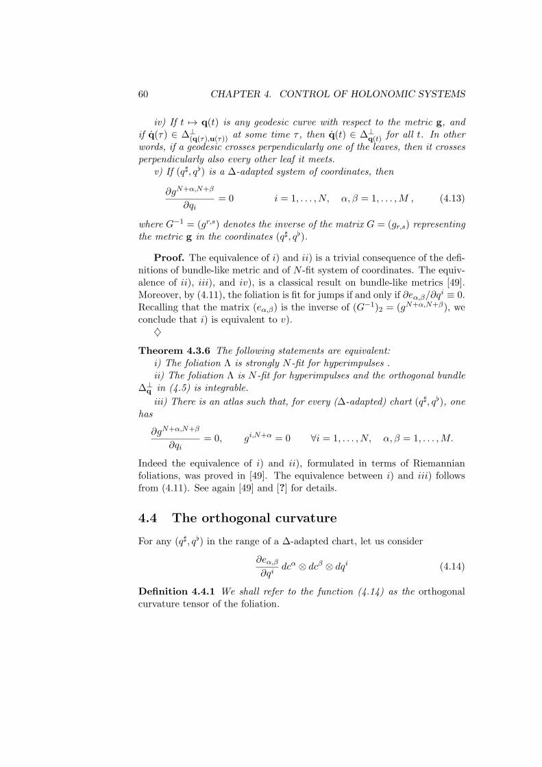
60 CHAPTER 4. CONTROL OF HOLONOMIC SYSTEMS
iv) If t 7→ q(t) is any geodesic curve with respect to the metric g, andif q(τ) ∈ ∆⊥
(q(τ),u(τ)) at some time τ , then q(t) ∈ ∆⊥q(t) for all t. In other
words, if a geodesic crosses perpendicularly one of the leaves, then it crossesperpendicularly also every other leaf it meets.
v) If (q♯, q) is a ∆-adapted system of coordinates, then
∂gN+α,N+β
∂qi= 0 i = 1, . . . , N, α, β = 1, . . . ,M , (4.13)
where G−1 = (gr,s) denotes the inverse of the matrix G = (gr,s) representingthe metric g in the coordinates (q♯, q).
Proof. The equivalence of i) and ii) is a trivial consequence of the defi-nitions of bundle-like metric and of N -fit system of coordinates. The equiv-alence of ii), iii), and iv), is a classical result on bundle-like metrics [49].Moreover, by (4.11), the foliation is fit for jumps if and only if ∂eα,β/∂q
i ≡ 0.Recalling that the matrix (eα,β) is the inverse of (G−1)2 = (gN+α,N+β), weconclude that i) is equivalent to v).
Theorem 4.3.6 The following statements are equivalent:i) The foliation Λ is strongly N -fit for hyperimpulses .ii) The foliation Λ is N -fit for hyperimpulses and the orthogonal bundle
∆⊥q in (4.5) is integrable.
iii) There is an atlas such that, for every (∆-adapted) chart (q♯, q), onehas
∂gN+α,N+β
∂qi= 0, gi,N+α = 0 ∀i = 1, . . . , N, α, β = 1, . . . ,M.
Indeed the equivalence of i) and ii), formulated in terms of Riemannianfoliations, was proved in [49]. The equivalence between i) and iii) followsfrom (4.11). See again [49] and [?] for details.
4.4 The orthogonal curvature
For any (q♯, q) in the range of a ∆-adapted chart, let us consider
∂eα,β∂qi
dcα ⊗ dcβ ⊗ dqi (4.14)
Definition 4.4.1 We shall refer to the function (4.14) as the orthogonalcurvature tensor of the foliation.

4.4. THE ORTHOGONAL CURVATURE 61
Lemma 4.4.2 The function in (4.14) is intrinsically defined with respect
to the foliation Λ. This means that if (q♯, q) is a ∆-adapted chart then
∂eα,β∂qi
=∂uγ
∂qN+α
∂qN+δ
∂qN+β
∂qj
∂qi∂eγ,δ∂qj
. (4.15)
Proof. Since (q♯, q) and (q, q) are ∆-adapted, the coordinate transfor-
mation (q♯, q) 7→ (q, q) satisfies ∂q
∂q = 0. Therefore,
gN+α,N+β =∂qN+α
∂qN+γ
∂qN+β
∂qN+δgN+γ,N+δ.
By inverting the matrices on both sides of the above identity one obtains
eα,β =∂qN+γ
∂QN+α
∂qN+δ
∂qN+βeγ,δ,
which implies (4.15), because q = q(q) is independent of q♯.
Remark 4.4.3 Although the quantity in (4.14) is not a tensor in the strictsense of the word, by (4.15) it still transforms like a tensor w.r.t. to changesof ∆-adapted coordinates. Hence, it is intrinsically defined in terms of thefoliation. By a slight abuse of language, we thus define (4.14) as the orthog-onal curvature tensor of the foliation Λ.
According to Theorem 4.3.5, the foliation Λ is N -fit for hyperimpulses ifand only if the the corresponding orthogonal curvature is identically equalto zero. We now give a geometric construction which clarifies the meaningof the coefficients ∂eα,β/∂q
i in (4.14), in the general case (see Figure 4.4).
In the following, given a tangent vector V ∈ T(q,u)(Q × U), we denoteby τ 7→ γV(τ) the geodesic curve starting from (q, u) with velocity V. Inother words,
γV(0) = (q, u) ,dγVdτ
(0) = V .
The exponential map is then defined by setting
Exp(q,u)(V).= γV(1).
This is well defined for all vectors V in a neighborhood of the origin.

62 CHAPTER 4. CONTROL OF HOLONOMIC SYSTEMS
Fix any point q ∈ Q and consider any non-zero vector V ∈ ∆⊥(q) . Con-
struct the geodesic curve that originates at q with speed V, namely
s 7→ γV(s).= Expq(sV) . (4.16)
Next, for each s = 0, consider the orthogonal space ∆⊥qs at the point qs =
γV(s). Assuming that s is sufficiently small, a transversality argument yieldsthe existence of a unique vector W ∈ ∆⊥
qs such that
ExpqsW = qs ∈ π−1(π(q)) . (4.17)
In other words, we are moving back to a point qs on the original leafπ−1(π(q)), following a second geodesic curve that is orthogonal to π−1(π(qs)).In general, qs = q. We claim that, setting σ
.= s2, the map
σ 7→ q√σ
defines a unique tangent vector Z(V) ∈ Tq . Moreover, the map V 7→ Z(V)is a homogeneous quadratic map from ∆⊥
q into the tangent space TqQ ⊂Tq(Q). In turn, this determines a unique symmetric bilinear mapping B :∆⊥
q ⊗ ∆⊥q 7→ TqQ such that B(V,V) = Z(V), namely
B(V1,V2).=
1
4Z(V1 + V2) −
1
4Z(V1 −V2) . (4.18)
The relation between the bilinear mapping (4.18) and the curvature ten-sor (4.14) can be best analyzed by using coordinates. Consider an orthonor-mal basis (J1, . . . , JM ) of ∆⊥
q , together with local ”U-orthonormal coordi-
nates” (q♯, q), constructed as [11]. If V = w1J1 + · · ·+wMJM , then by con-struction the point (qs,us) has coordinates (0, sw) = (0, . . . , 0, sw1, . . . , swM ).Let (q1w(s), . . . , qNw (s), 0, . . . , 0) be the coordinates of the point qs, (con-structed as in [11]). We have:
Theorem 4.4.4 The curve s 7→ qw(s) ∈ IRN is continuous and satisfies
lims→0
qiw(s)
s2=
1
2
M∑α,β=1
∂eα,β∂qi
wαwβ i = 1, . . . , N . (4.19)
We refer to [11] for the proof of this result, which is based on the con-
struction of U-orthonormal coordinates.
4.4. THE ORTHOGONAL CURVATURE 63
Figure 4.4: The geodesics involved in the computation of the orthogonalcurvature.

64 CHAPTER 4. CONTROL OF HOLONOMIC SYSTEMS

Chapter 5
Control of non-holonomicsystems
We consider a mechanical system as in Chapter 4 with, in addition, a nonholonomic constraint. This means that, at each point q ∈ Q, velocities mustbelong to a given subset of the tangent space. We shall consider ”linear”non holonomic constraints, which means that at each q ∈ Q the velocitieshave to lie in a subspace Γq ⊆ TqQ. The fact that the constraint is nonholonomic means that the distribution q → Γq is not integrable: there isno foliation whose leaves have the Γq as tangent spaces. (see AppendixA.) In other words, the constraints on the velocities cannot be deduced bydifferentiations from configuration constraints.
5.1 Non-holonomic systems with active constraintsas controls
Let N,M, ν be positive integers such that ν ≤ N . Let Q be an (N + M)-dimensional differential manifold, which will be regarded as the space ofconfigurations of a mechanical system.
Let Γ be a distribution on Q, i.e. a vector sub-bundle of the tangentspace TQ. Throughout the following, we consider trajectories t 7→ q(t) ∈ Qof the mechanical system which are continuously differentiable and satisfythe geometric constraint
q(t) ∈ Γq(t) . (5.1)
We do not assume Γ to be integrable, so that (5.1) is a non holonomicconstraint.
65

66 CHAPTER 5. CONTROL OF NON-HOLONOMIC SYSTEMS
In our model, the system will be controlled by means of an active (holo-nomic, time-dependent) constraint. To describe this constraint, let an M -dimensional differential manifold U be given, together with a submersion
π : Q 7→ U . (5.2)
The fibers π−1(u) ⊂ Q will be regarded as the states of the active constraint.The set of all these fibers can be identified with the control manifold U .
Let I be a time interval and let u : I 7→ U be a continuously differentiablemap. We say that a trajectory q : I → Q agrees with the control u(·) if
π q(t) = u(t) ∀t ∈ I . (5.3)
For each q ∈ Q, consider the subspace of the tangent space at q given by
∆q.= ker Tqπ .
Here Tqπ denotes the linear tangent map between the tangent spaces TqQand Tπ(q)U . Clearly, ∆ is the holonomic distribution whose integral mani-folds are precisely the fibers π−1(u).
5.1.1 General setting
1) The manifold Q is endowed with a Riemannian metric g = gq[·, ·],the so-called kinetic metric, which defines the kinetic energy T . Moreprecisely, for each q ∈ Q and v ∈ TqQ one has
T (q,v).=
1
2gq[v,v] . (5.4)
We shall use the notation v 7→ gq(v) to denote the isomorphism fromTqQ to T ∗
qQ induced by the scalar product gq[·, ·]. Namely, for everyv ∈ TqQ, the 1-form gq(v) is defined by
⟨gq(v),w⟩ .= gq[v,w] ∀w ∈ TqQ , (5.5)
where ⟨·, ·⟩ is the duality between the tangent space TqQ and thecotangent space T ∗
qQ.
If q ∈ Q and W ⊂ Tq, W⊥ denotes the subspace of Tq consisting ofall vectors that are perpendicular to every vector in W :
W⊥ .= v ∈ Tq | gq[v,w] = 0 ∀w ∈W .

5.1. NON-HOLONOMIC SYSTEMSWITH ACTIVE CONSTRAINTS AS CONTROLS67
For a given distribution E ⊂ TQ, the orthogonal distribution E⊥ ⊂TQ is defined by setting E⊥
q.= (Eq)⊥, for every q ∈ Q.
We use PE : TqQ → Eq to denote the orthogonal projection on Eq.Namely, for every v ∈ TqQ, PE(v) is the unique vector in Eq suchthat v − PE(v) ∈ E⊥
q .
2) Throughout the following, we shall assume that the holonomic distri-bution ∆ and the non-holonomic distribution Γ satisfy the tranversal-ity condition
∆q + Γq = TqQ ∀q ∈ Q . (5.6)
Notice that this is equivalent to
∆⊥ ∩ Γ⊥ = 0 . (5.7)
3) The mechanical system is subject to forces. In the Hamiltonian for-malism, these are represented by vertical vector fields on the cotangentbundle T ∗Q. We recall that, in a natural local system of coordinates(q, p), the fact that F is vertical means that its q-component is zero,namely F =
∑N+Mi=1 Fi
∂∂pi
.
4) The constraints (5.1) and (5.3) are dynamically implemented by reac-tion forces obeying
D’Alembert Principle: If t 7→ q(t) is a trajectory which satisfiesboth (5.1) and (5.3), and R(t) is the constraint reaction at a time t,then
R(t) ∈ ker(
∆q(t) ∩ Γq(t)
). (5.8)
In other words, regarding the reaction force R(t) as an element of thecotangent space T ∗
q(t)Q, one has
⟨R(t) , v⟩ = 0 ∀v ∈ ∆q(t) ∩ Γq(t) ⊆ Tq(t)Q . (5.9)
5.1.2 Equations of motion
For each q ∈ Q, we shall use g−1q to denote the inverse of the isomorphism
gq at (5.5). Moreover we define the scalar product on the cotangent spaceg−1q [·, ·] : T ∗
qQ× T ∗qQ 7→ IR by setting
g−1q [p, p]
.= gq [g−1
q (p), g−1q (p)] ∀ (p, p) ∈ T ∗
qQ× T ∗qQ .

68 CHAPTER 5. CONTROL OF NON-HOLONOMIC SYSTEMS
For every q ∈ Q, we shall use H(q, ·) to denote the Legendre transform ofthe map v → T (q,v), so that
H(q,p) =1
2g−1q [p,p]
(= T (q,g−1(p))
)∀ p ∈ T ∗
qQ . (5.10)
The map H : T ∗Q → IR will be called the Hamiltonian corresponding to thekinetic energy T .
Let (q) = (q♯, q) be local, ∆-adapted, coordinates on Q, and let (u) co-ordinates on U , such that the domain of the chart (q) is mapped by π into thedomain of the chart (u). We can assume, as usual, q(= (qN+1, . . . , qN+M )) =u(= (u1, . . . , qM )). From Classical Mechanics it follows that, given a smoothcontrol t 7→ u(t) (here regarded as a time-dependent holonomic constraintverifyng d’Alembert Hypothethis), the corresponding motion t 7→ (q, p)(t) onT ∗Q verifies the relations
q(t) =∂H
∂p(q(t), p(t))
p(t) = − ∂H
∂q(q(t), p(t)) + F (t, q(t), p(t)) +R(t)
q(t) = u(t)
p(t) ∈ gq(t)(Γq(t))
R(t) ∈ ker ∆q(t) + ker Γq(t) .
(5.11)
We have used H, F , R, and g to denote the local expressions of H, F, R, andg, respectively. For simplicity, we use the same notation for the distributionsΓ,∆ on Q and their local expressions in coordinates. Moreover, we usethe notation v 7→ gq(v) to denote the local expression of the isomorphismv 7→ gq(v).
The first two equations in (5.11) are the dynamical equations written inHamiltonian form. The first one yields the inverse of the Legendre transform.The third equation represents the (holonomic) control-constraint. Relyingon the fact that π is a submersion, we shall always choose local coordinates(qr) and (uα) such that qN+α = uα, for all α = 1, . . . ,M . We thus regardthis equation as prescribing a priori the evolution of the last M coordinates:qN+1, . . . , qN+M . The fourth relation in (5.11) is the Hamiltonian version ofthe non holonomic constraint (5.1). The fifth relation is clearly equivalentto (5.8), i.e. it represents d’Alembert’s Principle.

5.2. ORTHOGONAL DECOMPOSITIONS 69
Remark 5.1.1 Although a global, intrinsic formulation of these equationscan be given (see [29]) we are here mainly interested in their local coordinate-wise expression. Indeed, a major goal of our analysis is to understand thefunctional dependence on the time derivative u of the control.
The special case where no active constraints are present can be obtainedby taking ∆ ≡ T ∗Q, i.e. ker(∆) = 0. In this case, (5.11) reduces tothe standard Hamiltonian version of the dynamical equations with non-holonomic constraints, namely
q(t) =∂H
∂p(q(t), p(t))
p(t) = − ∂H
∂q(q(t), p(t)) + F (t, q(t), p(t)) +R(t)
p(t) ∈ gq(t)(Γq(t))
R(t) ∈ ker Γq(t) ,
(5.12)
5.2 Orthogonal decompositions of the tangent andthe cotangent bundles
To derive a set of equations describing the constrained motion, it will beconvenient to decompose both the tangent bundle TQ and the cotangentbundle T ∗Q as direct sums of three suitable vector sub-bundles. We recallthat Q is a manifold of dimension N +M , while ∆ and Γ are distributionson Q, having dimensions N and N +M − ν, respectively.
5.2.1 Tangent bundle
Definition 5.2.1 For every q ∈ Q, we define the following three subspacesof TqQ.
(TqQ)I.= ∆q∩Γq , (TqQ)II
.= Γ⊥
q , (TqQ)III.= (∆q∩Γq)⊥∩Γq .
(5.13)
Proposition 5.2.1 For each q ∈ Q, the three subspaces in (5.13) are mu-tually orthogonal and span the entire tangent space, namely
TqQ = (TqQ)I ⊕ (TqQ)II ⊕ (TqQ)III . (5.14)

70 CHAPTER 5. CONTROL OF NON-HOLONOMIC SYSTEMS
Moreover,
(TqQ)I ⊕ (TqQ)III = Γ . (5.15)
If the transversality condition (5.6) holds, then the above subspaces havedimensions
dim(TqQ)I = N − ν , dim(TqQ)II = ν , dim(TqQ)III = M .(5.16)
Proof. The orthogonality of the subspaces (TqQ)I and (TqQ)II is im-mediately clear from the definitions. Observing that(
(TqQ)I⊕(TqQ)II
)⊥=(
(TqQ)I
)⊥∩(
(TqQ)II
)⊥= (∆q∩Γq)⊥∩Γq = (TqQ)III ,
we obtain the orthogonal decomposition (5.14). In particular, this implies
(TqQ)I ⊕ (TqQ)III =(
(TqQ)II
)⊥= Γq .
Finally, if (5.6) holds, then
dim(∆q∩Γq) = dim(∆q)+dim(Γq)−dim(TqQ) = N+(N+M−ν)−(N+M) = N−ν .
Moreover, dim(
(TqQ)II
)= dim(TqQ) - dim(Γq) = ν. The last equality in
(5.16) now follows from (5.14).
For J ∈ I, II, III, the perpendicular projection onto the subspace(TQ)J will be denoted by
PJ : TqQ 7→ (TqQ)J . (5.17)
Remark 5.2.2 Under the assumption (5.6), the third subspace in the de-composition (5.14) can be equivalently written as
(TqQ)III = PΓ(∆⊥q ).
Indeed, for any vector v ∈ TqQ one has v ∈ PΓ(∆⊥q ) iff
v ∈ Γq ∩ (∆⊥q + Γ⊥
q ) = Γq ∩ (∆q ∩ Γq)⊥.

5.3. A CLOSED SYSTEM OF CONTROL EQUATIONS 71
5.2.2 Cotangent bundle
Thanks to the isomorphism g : TQ 7→ T ∗Q defined at (5.5), one can use(5.14) to obtain a similar decomposition of the cotangent bundle as thedirect sum of three vector bundles:
T ∗Q = (T ∗Q)I ⊕ (T ∗Q)II ⊕ (T ∗Q)III , (5.18)
where, for J ∈ I, II, III,
(T ∗qQ)J
.= gq
((TqQ)J
). (5.19)
We denote by P∗J : T ∗
qQ → (T ∗qQ)J the perpendicular projection w.r.t. the
metric g−1. The above construction yields
P∗J = g PJ g−1 . (5.20)
In view of Proposition 5.2.1 one obtains:
Proposition 5.2.2 If the transversality condition (5.6) holds, then
dim(
(T ∗qQ)I
)= N−ν , dim
((T ∗
qQ)II
)= ν , dim
((T ∗
qQ)III
)= M .
(5.21)Moreover, for every q ∈ Q the three subspaces (T ∗
qQ)I , (T∗qQ)II , (T
∗qQ)III
are pairwise orthogonal (w.r.t. the metric g−1). In particular, (T ∗qQ)II =
ker(Γq).
5.3 A closed system of control equations
The following result, providing different ways to express the constraint (5.1),is straightforward.
Lemma 5.3.1 Let t 7→ q(t) ∈ Q be a C1 map. Let p(t).= g(q(t)). More-
over, setqII(t)
.= PII(q(t)), pII
.= P∗
II(p(t)).
Then the non-holonomic constraint q(t) ∈ Γq(t) can be expressed in any ofthe following equivalent forms:
p(t) ∈ g(Γq(t)) ⇐⇒ qII(t) = 0 ⇐⇒ pII(t) = 0. (5.22)

72 CHAPTER 5. CONTROL OF NON-HOLONOMIC SYSTEMS
On a given, natural chart (q, p) on T ∗Q, and for J ∈ I, II, III, we de-note by P ∗
J the (q-dependent) matrix representing the projection P∗J . In this
coordinate system, the components of the force and of the constraint reac-tion will be denoted as FJ
.= P ∗
J F and RJ.= P ∗
J R. For every J = I, II, III,consider the bilinear (q-dependent, possibly not symmetric), IRN+M -valuedmap
(p, p) 7→ θJ [p, p].=(
[θJ ]r,sℓ prps
)ℓ=1,...,N+M
, (5.23)
where
[θJ ]r,sℓ.=
N+M∑i=1
(∂(P ∗
J )rℓ∂qi
gi,s − 1
2
∂gr,s
∂qi(P ∗
J )iℓ
). (5.24)
The following result will be essential in deriving the equations of motions,relative to the bundle decomposition introduced above.
Lemma 5.3.2 Let t 7→ (q, p)(t) be a C1 map. For J ∈ I, II, III, define
pJ(t).= P ∗
J p(t) , (5.25)
so that p(t) = pI(t) + pII(t) + pIII(t) for all t. Let t 7→ R(t) be a continuousmap. Then the following statements are equivalent.
A) The map p(·) satisfies the equation
p(t) = − ∂H
∂q(q(t), p(t)) + F (t, q(t), p(t)) +R(t) . (5.26)
B) The maps (pI)(·), (pII)(·), (pIII)(·) satisfy the system
pJ(t) = θJ [p(t), p(t)]+FJ(t, q(t), p(t))+RJ(t), J ∈ I, II, III .(5.27)
Remark 5.3.1 In general θJ [p, p] /∈ P ∗J (IRN+M ). Indeed, the derivative pJ
may not be contained in the sub-space P ∗J (IRN+M ).
Proof of Lemma 5.3.2. Assume that B) holds. By summing the threeequations in (5.27) one obtains
p(t) = pI(t) + pII(t) + pIII(t)
= θI [p(t), p(t)] + θII [p(t), p(t)] + θIII [p(t), p(t)] + F (t, q(t), p(t)) +R(t)
= (P ∗I + P ∗
II + P ∗III)
(−∂H∂q
(q(t), p(t))
)+ F (t, q(t), p(t)) +R(t)
= −∂H∂q
(q(t), p(t)) + F (t, q(t), p(t)) +R(t)

5.3. A CLOSED SYSTEM OF CONTROL EQUATIONS 73
where we have exploited the identities
P ∗I + P ∗
II + P ∗III = Id,
∂P ∗I
∂q+∂P ∗
II
∂q+∂P ∗
III
∂q=
∂(Id)
∂q= 0.
This proves the validity of the differential equation (5.26).
Conversely, assume that A) holds. Then, for J ∈ I, II, III one has
pJ =d
dt(P ∗
J p) =(∂P ∗
J
∂q· q(t)
)p(t) + P ∗
J p(t)
=(∂P ∗
J
∂q· g−1(p)
)p(t) + P ∗
J
(−1
2
∂g−1
∂q[p(t), p(t)] + F (t, q(t), p(t)) +R(t)
)= θJ [p(t), p(t)] + FJ(t, q(t), p(t)) +RJ(t) .
This proves the validity of the differential equations for pI , pII , and pIII in(5.27).
5.3.1 The system without control-constraints
The equations of motion for a non-holonomic system with external forcescan be found in several textbooks, see for example [1, 5, 4]. We review herea form of these equations, relative to decompositions (5.14) and (5.18)
Theorem 5.3.1 Let t 7→ q(t) be a continuously differentiable path and setp(t)
.= g(q(t)). Then the path (q, p)(·) satisfies the non-holonomic equations
(5.12) (with no active constraints) if and only if it is a solution of
q = g−1(p)
pI = θI [p, p] + FI
pII = 0
pIII = θIII [p, p] + FIII .
(5.28)
Proof. Assume that the relations (5.12) hold. For every J ∈ I, II, IIIconsider the projection qJ(t)
.= PJ q(t), where PJ is the coordinate represen-
tation of the projection PJ . By Lemma 5.3.1 one has qII(t) = 0 and hence

74 CHAPTER 5. CONTROL OF NON-HOLONOMIC SYSTEMS
pII(t) = 0, for every t. Therefore, the third and the first equation in (5.28)are straightforward:
pII ≡ 0 , q = g−1(pI + pIII) = g−1(p).
Next, since P ∗I (IRN+M ) ⊕ P ∗
III(IRN+M ) = g(Γ), the last relation in (5.12)
(i.e. the d’Alembert condition) implies P ∗I (R(t)) = P ∗
III(R(t)) = 0 for allt. Using the second equation in (5.12 and Lemma 5.3.2, for J ∈ I, III wethus obtain
pJ = θJ [p, p] + FJ(t) .
This proves the validity of the differential equations for pI and pIII in (5.28).
Conversely, let the equations in (5.28) hold, with θI , θIII defined as in(5.23)-(5.24).
The third equation in (5.12) follows from pII = 0. In particular p =pI + pIII . The first equation in (5.12) follows by
q = g−1(pI + pIII) = g−1(p) =∂H
∂p.
If the constraint reaction R(t) is defined by
R(t).= p(t) +
∂H
∂q(q(t), p(t)) − F (t, q(t), p(t)), (5.29)
then the second equation in (5.12) is trivially satisfied.
We claim that the fourth relation in (5.12) also holds, namely R(t) ∈ker Γq(t) for every time t. Indeed, by Lemma 5.3.2, (5.29) is equivalent to
pI(t) = θI(p(t), p(t)) + FI(t, q(t), p(t)) +RI(t)
pII(t) = θII(p(t), p(t)) + FII(t, q(t), p(t)) +RII(t)
pIII(t) = θIII(p(t), p(t)) + FIII(t, q(t), p(t)) +RIII(t) .
Hence, by the second and third equations in (5.28) one hasRI(t) = RIII(t) =0. This implies R(t) ∈ P ∗
II(IRN+M ) = ker Γq(t).

5.3. A CLOSED SYSTEM OF CONTROL EQUATIONS 75
5.3.2 The non-holonomic system with control-constraints
In this section we write the equations of motion controlled by means of activeconstraints (5.11) in an equivalent form, as a closed system of controlleddifferential equations, supplemented by algebraic relations.
Since π : Q 7→ U is a submersion, the transversality assumption (5.6)implies that, for every q ∈ Q, the restriction of the tangent map Tqπ to thesubspace (TqQ)III is an isomorphism from (TqQ)III onto TUπ(q). We shalluse h to denote the inverse of this isomorphism, and define k
.= g h.
We now choose local coordinates (q, p) on T ∗Q, together with coordinatesu on U , such that
qN+1 = u1 , . . . , qN+M = uM . (5.30)
The expressions of h and k in local coordinates will be denoted by h andk, respectively. We recall that the bilinear map θI was defined at (5.23)-(5.24). In the following, it is understood that the maps u, q should takevalues within the domains of the respective charts.
Theorem 5.3.2 Let I be a time interval and let u : I → IRM be a C1
control function. Let q : I 7→ IRN be a C1 path and set p(t).= g(q(t)).
Then the path (q, p) : I → T ∗Q satisfies the non holonomic equations (5.11)(with constraints as controls) if and only if the following two conditions aresatisfied.
(i) Setting pJ(t).= P ∗
J (p(t)), for every t ∈ I one has
q = g−1(pI) + h(u)
pI = θI [pI + k(u) , pI + k(u)] + FI
pII = 0
pIII = k(u) .
(5.31)
(ii) At some time t0 ∈ I one has qN+α(t0) = uα(t0) for all α = 1, . . . ,M .
Proof. 1. Assume that all relations in (5.11) are satisfied. By (5.22)the fourth relation in (5.11) implies pII = 0. Using the third equation in

76 CHAPTER 5. CONTROL OF NON-HOLONOMIC SYSTEMS
(5.11) we obtainpIII = g(qIII) = g(h(u)) = k(u)
p = pI + pIII = pI + k(u)
q(t) = g−1(p) = g−1(pI + k(u)) = g−1(pI) + h(u) .
(5.32)
Finally, the fifth relation in (5.11), i.e. the d’Alembert condition, impliesP ∗I R(t) = 0. Hence, by the second equation on (5.11) and Lemma 5.3.2, we
obtain
pI =d
dt
(P ∗I p)
= θI [p, p] + FI = θI [pI + k(u), pI + k(u)] + FI .
This yields the second equation in (5.31).
2. Viceversa, assume that all the relations in (5.31) hold, and let us setp.= pI + k(u). By (5.22), the equation pII = 0 implies the fourth relation
in (5.11). Moreover, from the first equation in (5.31) and the identities in(5.32) we obtain
q = g−1(pI) + h(u) = g−1(p) =∂H
∂p(q, p) .
By defining
R(t).= p+
∂H
∂q(q, p) − F (t, q(t), p(t)), (5.33)
the second equation in (5.11) is clearly satisfied. It remains to check the fifthequation in (5.11), namely R(t) ∈ ker ∆q(t)+ker Γq(t). Since by constructionker ∆+ker Γ = (T ∗Q)II+(T ∗Q)III , this is equivalent to proving that RI = 0.By Lemma 5.3.2, (5.33) is equivalent to the three equalities
pI = θI [p, p] + FI +RI
pII = θII [p, p] + FII +RII
pIII = θIII [p, p] + FII +RIII .
(5.34)
By subtracting the second equation in (5.31) from the first identity in(5.34) we obtain RI(t) = 0.

5.3. A CLOSED SYSTEM OF CONTROL EQUATIONS 77
Remark 5.3.2 In order to express more clearly the functional dependenceon u, let us write the equations (5.31) in the form
q = g−1(pI) + h(u)
pI = θI [pI , pI ] + Υ[pI , u] + Ψ[u, u] + FI
pII = 0
pIII = k(u) ,
(5.35)
where
Υ[pI , k(u)].= θI [pI , k(u)]+θI [k(u) , pI ], Ψ[u, u]
.= θI [k(u) , k(u)].
(5.36)
5.3.3 The case without non-holonomic constraints
When there is no presence of non-holonomic constraints, that is, whenΓq = TQ for all q ∈ Q, the equations in (5.35) should reduce to (4.9),the controls system we have introduced in Chapter 4. In fact, we had notproved the validity of those equations and we have referred to the fact thatthey could be obtained as a degenerate case (ν = 0) of the case with nonholonomic constraints. We leave to the reader the explicit deduction of (4.9)from (5.35). While this is a bit laborious, we point out that it reduces toelementary steps based on basic matrix computations and on the followingcrucial issues:
1. when ν = 0, the decomposition T ∗Q = (T ∗Q)I ⊕ (T ∗Q)II ⊕ (T ∗Q)IIIreduces to (T ∗Q)I = g(∆), (T ∗Q)II = 0, (T ∗Q)III = g(∆⊥),g(∆) ⊕ g(∆⊥).
2. In any natural system of coordinates on T ∗Q connected with ∆-adaptedcoordinates (q♯, q), the projection P∗
I reduces to the projection on thefirst n-dimensional component, namely it is given by the (N + M) ×(N + M) constant matrix where upper left N × N minor coincideswith the unit matrix and the other digits are zero.
3. The space ∆⊥q is generated my the last M columns of the matrix g
representing the kinetic metric g.
Remark 5.3.3 Notice that the simplifying issue in passing from the casewith non holonomic constraints to that without such constraints relies just

78 CHAPTER 5. CONTROL OF NON-HOLONOMIC SYSTEMS
on the fact that (in all ∆- adapted coordinates) the projection P∗I is constant.
Hence, the only possible occurrence of the u-quadratic term in the controlequations is due to the non vanishing of the orthogonal curvature introducedin Chapter 4. On the contrary, in the general case, an extra occurrence ofthe quadratic term is due to the fact that in general the projection P∗
I isnot constant, which is indeed a manifestation of the non-holonomy of theadditional constraint q ∈ Γq.
5.4 A control system with a reduced number ofequations
Let q = (q1, . . . , qN+M ) be ∆-adapted coordinates on a open set Ø ⊆ Q , sothat
∆ = span ∂
∂q1, . . . ,
∂
∂qN
.
The main goal of this section is to write the equations of motion in terms ofthese state coordinates, together with additional coordinates ξ1, . . . , ξN+M
corresponding to suitable bases of the cotangent bundle T ∗Q, decomposedas in (5.18). It will turn out that the number of control equations can bereduced to 2N − ν. In fact, the relevant equations will involve only thevariables q1, . . . , qN , ξ1, . . . , ξN−ν .
Consider a family V1, . . . ,VN+M of smooth, linearly independent vec-tor fields on Q, such that
(TqQ)I = spanV1(q), . . . ,VN−ν(q)
,
(TqQ)II = spanVN−ν+1(q), . . . ,VN (q)
,
(TqQ)III = spanVN+1(q), . . . ,VN+M (q)
.
(5.37)
Throughout the following, we assume that the vectors V1, . . . ,VN−ν,which generate (TqQ)I , are orthogonal, i.e.
g[Vr,Vs] = 0 ∀r, s ∈ 1, . . . , N − ν, r = s . (5.38)
In addition, for i = 1, . . . , N +M , we define the basis of cotangent vectors
Ωi.=
g(Vi)g[Vi, Vi]
, (5.39)
5.4. A CONTROL SYSTEMWITH A REDUCEDNUMBEROF EQUATIONS79
By (5.19), this yields
(T ∗qQ)I = span
Ω1(q), . . . ,ΩN−ν(q)
,
(T ∗qQ)II = span
ΩN−ν+1(q), . . . ,ΩN (q)
,
(T ∗qQ)III = span
ΩN+1(q), . . . ,ΩN+M (q)
.
By (5.40) and (5.39), the differential forms Ω1, . . . ,ΩN−ν are mutuallyorthogonal with respect to the metric g−1, namely
g−1[Ωr, Ωs] = 0 ∀r, s ∈ 1, . . . , N − ν, r = s . (5.40)
Moreover, the basisΩ1(q), . . . ,ΩN−ν(q)
is dual to the basis
V1(q), . . . ,VN−ν(q)
,
i.e.
⟨Ωr, Vs⟩ = δr,s ∀r, s = 1, . . . , N − ν.
This choice of orthogonal bases makes it easy to compute the projections PIand P∗
I . Indeed, for any tangent vector w and any cotangent vector p onehas
PI(w) =N−ν∑ℓ=1
⟨Ωℓ, w⟩ Vℓ =N−ν∑ℓ=1
g[w,Vℓ]g[Vℓ,Vℓ]
Vℓ, (5.41)
P∗I (p) =
N−ν∑ℓ=1
⟨p, Vℓ⟩Ωℓ =N−ν∑ℓ=1
g−1[p,Ωℓ]
g−1[Ωℓ, Ωℓ]Ωℓ . (5.42)
In the following, to simplify notation, whenever repeated indices takingvalues from 1 to N+M are summed, the summation symbol will be omitted.On the other hand, summations ranging over a smaller set of indices will beexplicitly written. Let g = (gr,s) be the matrix representing the Riemannianmetric g in the q-coordinates. In turn, the inverse matrix g−1 = (gr,s)represents the metric g−1 on the cotangent space.
For ℓ = 1, . . . , N + M , let V 1ℓ, . . . , V
N+Mℓ be the q-components of Vℓ,
so that Vℓ = V iℓ∂∂qi
. If the (column) vector v ∈ IRN+M yields the coor-dinate representation of v, then by (5.41) the projected vector PI(v) hascoordinates PI v, where the (N +M) × (N +M) matrix PI is defined by
(PI)sr.=
N−ν∑ℓ=1
gr,kVkℓV
sℓ
gi,jV iℓV j
ℓr, s = 1, . . . , N +M .

80 CHAPTER 5. CONTROL OF NON-HOLONOMIC SYSTEMS
Similarly, let Ωr,1, . . . ,Ωr,N+M be the components of Ωr, so that Ωr =Ωr,sdq
s. If the (row) vector p ∈ IRM+N yields the coordinate representationof the covector p, then by (5.42) the projected the vector P∗
I (p) has coordi-nates given by pP ∗
I , where the (N + M) × (N + M) matrix P ∗I is defined
by
(P ∗I )rs
.=
N−ν∑ℓ=1
gr,k Ωℓ,k Ωℓ,s
gi,j V iℓ V j
ℓ. (5.43)
In order to derive a reduced form of the system (5.31), we need to writean explicit expression of the (q-dependent) matrices h and k. Let us definethe (N +M) ×M matrix VIII and the M ×M matrix V III
III by setting
VIII.=(V r
N+α
), V III
III.=(V N+β
N+α
)Here and in the sequel, Greek indices such as α, β range from 1 to M ,while Latin indices such as r, s range from 1 to N + M . Recalling theidentities (5.30), it is easy to check that the injective linear map h : TUπ(q) 7→(TqQ)III ⊂ TqQ introduced in Section 5.3.2 is represented by the (N+M)×M matrix
h = VIII ·(V III
III
)−1.
In turn, the linear map k(·) = g(h(·)) is represented by the (N +M)×Mmatrix
k.= g · h = g · VIII ·
(V III
III
)−1.
5.4.1 Reduction of the number of equations
It clearly suffices to derive equations describing the first N components(q1, , . . . , qN ) of q, because by (5.30) the last M components coincide withthose of the control u. This already reduces the number of differential equa-tions in (5.31) from 2N + 2M to 2N +M .
Relying on the fact that the projection P∗I takes values in the subbundle
(T ∗Q)I , which has dimension N−ν, one can reduce the number of equationsto 2N − ν, as shown in the following theorem.
Theorem 5.4.1 Let (q, p, u)(·) be as in Theorem 5.3.2. Moreover, let (ξ, η, λ)be the components of p = pidq
i w.r.t. the frame Ω1, . . . ,ΩN+M, so that
p(t) =
N−ν∑ℓ=1
ξℓ(t)Ωℓ +
N∑ℓ=N−ν+1
ηℓ(t)Ωℓ +
N+M∑ℓ=N+1
λℓ(t)Ωℓ .

5.4. A CONTROL SYSTEMWITH A REDUCEDNUMBEROF EQUATIONS81
Then the curve t 7→ (q(t), pI(t), pII(t), pIII(t), u(t)) satisfies the control sys-tem (5.35) if and only if the curve t 7→ (q(t), ξ(t), η(t), λ(t), u(t)) is a solutionof
qr =
N−ν∑ℓ=1
W rℓξℓ + hrN+αu
α r = 1, . . . , N
ξm = θm[ξ, ξ] + Υm [ξ , u] + Ψm[u, u] + Fm m = 1, . . . , N − ν
qN+α = uα α = 1, . . . ,M
η = 0
λ = (VIII)t · k · u
(5.44)where: i) for every ℓ = 1, . . . , N − ν, and r = 1, · · · , N we have set W r
ℓ.=
V rℓ/(gh,kV
hℓV
kℓ); ii) the superscript t denotes transposition; and iii) for
every m = 1, . . . , N − ν,
θm[ξ, ξ].=∑N−ν
a,b=1 θa,bm ξaξb, with
θa,bm.=
[θI ]r,si Ωr,aΩs,b −
N∑j=1
∂Ωi,a
∂qjgj,sΩs,b
V im,
Υm [ξ , u].=∑N−ν
a=1 Υaα,m ξa u
α, with
Υaα,m
.=
Υrα,i Ωr,a −
∂Ωi,a
∂qN+α−
N∑j=1
∂Ωi,a
∂qjV i
mhjN+α
V im,
Ψm [w, w].= Ψα,β,mw
αwβ, with
Ψα,β,m.= Ψα,β,iV
im , Fm
.= FiV
im .
(5.45)

82 CHAPTER 5. CONTROL OF NON-HOLONOMIC SYSTEMS
Proof. Recalling that pI i =∑N−ν
ℓ=1 ξℓΩi,ℓ, one obtains
pi =
N−ν∑ℓ=1
ξℓΩi,ℓ +
N−ν∑ℓ=1
N∑j=1
ξℓ∂Ωi,ℓ
∂qjqj
=
N−ν∑ℓ=1
ξℓΩi,ℓ +
N−ν∑ℓ=1
N∑j=1
(ξℓ∂Ωi,ℓ
∂qjgjrpIr + hjN+αu
α
)+
N−ν∑ℓ=1
M∑α=1
ξℓ∂Ωi,ℓ
∂qN+αuα
=
N−ν∑ℓ=1
ξℓΩi,ℓ +
N−ν∑ℓ=1
N∑j=1
(ξℓ∂Ωi,ℓ
∂qjgjr(
N−ν∑ℓ=1
ξℓΩi,ℓ) + hjN+αuα
)+
N−ν∑ℓ=1
M∑α=1
ξℓ∂Ωi,ℓ
∂qN+αuα .
(5.46)Since Ωi,rV
im = δr,m, for all r,m = 1, . . . , N − ν, by (5.46) and the second
equation in (5.31) one obtains the equations for the adjoint variable ξ. Theother equations in (5.44) are trivially derived by substitution.
5.5 Continuity properties of the input-output map
We now examine the connections between the following properties:
i) The continuity of the input-output functional u(·) 7→ (q(·), p(·)).
ii) The vanishing of the “centrifugal” term Ψ[u, u] in (5.36).
iii) The invariance of the distribution Γ∩(Γ∩∆)⊥ in Γ-constrained inertialmotions.
As in Section 2, T will denote the kinetic energy associated with themetric g, defined at (5.4), while Γ denotes a non-holonomic distribution onthe manifold Q.
Definition 5.5.1 Let I be a time interval. A C2 map q : I → Q will becalled a free inertial motion if, in any set of coordinates, its local expressionq(·) provides a solution to the Euler-Lagrange equations
d
dt
∂T∂q
− ∂T∂q
= 0. (5.47)
Definition 5.5.2 A C2 map q : I → Q will be called a Γ-constrained inertialmotion if, in any set of coordinates, its local expression q(·) is a solution of
d
dt
∂T∂q
− ∂T∂q
∈ ker Γ (5.48)

5.5. CONTINUITY PROPERTIES OF THE INPUT-OUTPUT MAP 83
and satisfies non holonomic constraints
q ∈ Γ. (5.49)
Definition 5.5.3 Let S ⊆ TQ be any set. We say that S is invariant forthe free inertial flow, (or equivalently: inertially invariant), if, for every freeinertial motion q : I → Q such that (q, q)(t0) ∈ S for some t0 ∈ I, one has
(q, q)(t) ∈ S ∀t ∈ I. (5.50)
Definition 5.5.4 Let S ⊆ T Q be any set. We say that S is invariant forthe Γ-constrained inertial flow, (or equivalently: Γ-inertially invariant), if,for every Γ-constrained inertial motion q : I → Q such that (q, q)(t0) ∈ Sfor some t0 ∈ I, one has
(q, q)(t) ∈ S ∀t ∈ I. (5.51)
Theorem 5.5.1 The following conditions are equivalent:
1) If F ≡ 0, for every C1 control u(·) and every solution q(·) of the controldifferential equation (on Q)
q = h(u),
the map
t 7→ (q(t), p(t)).=(q(t) , k(u(t))
)is a solution of (5.31). Equivalently, pI(t) = 0 for all t ∈ I.
2) For every local chart (q) the (vector-valued) quadratic form Ψ definedat (5.36) vanishes identically.
3) For every local chart (q), the (vector-valued) quadratic form v 7→θI [v, v] in (5.23) vanishes on the subspace P ∗
III(IRN+M ).
4) The sub-bundle (TQ)III = Γ ∩ (Γ ∩ ∆)⊥ is Γ-inertially invariant.
Proof. Let a continuously differentiable control u(·) be given. If condition2) holds true then, by the linearity of the equation for pI , there is a solution(q, p)(·) of (5.31) such that pI ≡ 0. This solution verifies the equation for q,so that q = h(u) and p = pIII = g(q) = k(u). Hence condition 1) is verified.Conversely, if Ψ is not identically zero, then it is not possible that for everyinitial condition and every control there exists a solution (q, p) such thatpI ≡ 0. Hence conditions 1) and 2) are equivalent.

84 CHAPTER 5. CONTROL OF NON-HOLONOMIC SYSTEMS
The equivalence of 1) and 3) follows directly by the definition of θI andΨ.
Finally, 1) holds true if and only if 4) is verified: indeed, on one handit is well known that the equations (5.31) can be (locally) written in theLagrangian form (5.48)-(5.49). On the other hand the condition pI = 0 isequivalent to q ∈ Γ ∩ (Γ ∩ ∆)⊥.
5.6 A geometric interpretation of the quadraticterm
Let us fix u ∈ U , w ∈ TuU and let u : V → IRM be a chart defined on aneighborhood of u.
Let u = (u1, . . . , uM ) be the coordinates of u, and let the M -tuple w =(w1, . . . , wM ) be defined by w =
∑Mα=1 w
α ∂∂uα . Fix a map η : [0, 1] → IR of
class C1 such that
∥η∥2 = 1, η(0) = η(1) = 0, η(0+) = η(1−) (5.52)
Finally, let the family of curves
uϵ : [0, ϵ] → U ϵ ∈ [0, 1]
be such that for every ϵ ∈]0, 1] (the image uϵ([0, 1]) is entirely included inthe coordinates’ domain V and) the local expression uϵ(·) of uϵ is given by :
uϵ(t).= u+ ϵη(t/ϵ)w ∀t ∈ [0, 1] (5.53)
Notice that
uϵ(0) = w ∀ϵ ∈]0, 1],
∫ ϵ
0uϵ(s)ds = 0,
∫ ϵ
0η2(t/ϵ)dt = ϵ (5.54)
Now choose q ∈ Q such that u = π(q). For every ϵ ∈]0, 1], let us considerthe solution (qϵ,pϵ) : [0, ϵ] → T ∗Q of the control system locally expressedby (5.35), with initial condition (qϵ(0),pϵ(0)) = (q,g(h · w)). 1
Let us consider the continuous curve b : [0, 1] → Q
ϵ 7→ b(ϵ).= qϵ(ϵ)
Remark 5.6.1 The image b([0,1]) lies on the leaf π−1(u) , i.e. π (b(ϵ)) =u, for all ϵ ∈ [0, 1].
1See Section 5.4 for the definition of the isomorphism h.

5.6. QUADRATIC TERM 85
Theorem 5.6.1 The map b is twice differentiable at ϵ = 0 and, for anynatural system of coordinates (q, v) one has
db
dϵ(0) = 0
d2 b
dϵ2(0) = gjiΨi[w,w]
∂
∂vj
where the Ψi’s are the components of the (IRN+M -valued) quadratic form Ψdefined in (5.36).
Definition 5.6.2 In view of Theorem 5.6.1, for every q ∈ Q let us call thebilinear map
w → Ψi[w,w]gij∂
∂vj
(=d2b
dϵ2(0)
)the curvature of the Γ-constrained orthogonal bundle (TqQ)III .
Proof of Theorem 5.6.1. Let local coordinates (q) and (u) be chosennear q and u = π(q), respectively. It is not restrictive to assume thatq(q) = 0, u(u) = 0. For every r = 1, . . . , N + M let vr
.= hrαw
α, so that,hw = v = vr ∂
∂qr ∈ (TqQ)III). Let qϵ be the coordinate representation of
the curve qϵ. For every s ∈ [0, ϵ] let us set pϵ(s).= g(qϵ) (where the matrix
g is evaluated at (qϵ(s))), and let us notice that (qϵ, pϵ)(·) verify
q = pI · g−1(q) + h · u
pI = θI [pI + k(u) , pI + k(u)]
pII = 0
pIII = k(u)
q(0) = 0
(pI , pII , pIII)(0) = (0, 0, kw).
(5.55)
where pJ.= PJ(p), for J = I, II, III. In particular, since the derivatives
uϵ are equi-bounded, by standard estimates it follows that the trajectories

86 CHAPTER 5. CONTROL OF NON-HOLONOMIC SYSTEMS
(qϵ, pϵ) are equi-bounded as well. Therefore, since pI(0) = 0,
qϵ(ϵ) =
∫ ϵ
0
((pϵ)I(s) · g−1(qϵ(s)) + h(qϵ(s)) · uϵ(s)
)ds =
∫ ϵ
0
((pϵ)I(0) · g−1(0) + h(0) · uϵ(s) + o(ϵ)
)ds =
o(ϵ2) + h(0) ·∫ ϵ
0uϵ(s) ds = o(ϵ2)
(5.56)
and
qϵ(ϵ) − v = g−1(qϵ(ϵ)
)· pϵ(ϵ) − g−1
((0))· (k(0) · w) =
g−1(qϵ(ϵ)
)·∫ ϵ
0θI(qϵ(s))
[pI ϵ(s) + k(qϵ(s)) · uϵ(s) , pI ϵ(s) + k(qϵ(s)) · uϵ(s)
]ds =
g−1 (0) ·∫ ϵ
0θI(0)
[k(0) · uϵ(s) , k(0) · uϵ(s)
]ds+ o(ϵ2) =
g−1 (0) · θI(0)[k(0) · w , k(0) · w]
∫ ϵ
0η2(t/ϵ) dt+ o(ϵ2)
= ϵg−1 (0) · θI(0)[k(0) · w , k(0) · w] + o(ϵ2)(5.57)
By (5.56) and (5.57), if b(·) is the local expression of b(·), we get
db
dϵ= lim
ϵ→0
(qϵ(ϵ), qϵ(ϵ)
)− (0, v)
ϵ=(
0 , g−1 (0) ·(θI(0)
[k(0) · w , k(0) · w
])=(
0 , g−1 (0) · Ψ(0)[w ,w
])= (0, g1,iΨi[w,w], . . . , gN+M,iΨi[w,w])

Chapter 6
Stabilization bycontrol-constraints
6.1 Holonomic systems
Let us recall the control equations from Chapter 4. LetG = (gr,s)r,s=1,...,N+M
be the matrix that represents the covariant inertial tensor in a given coor-dinate chart (q♯, q). In particular, the kinetic energy of the whole systemat a state (q♯, q) with velocity (v, w) ∈ IRN+M is given by
T =1
2gi,j(q
♯, q)vivj + gi,N+α(q♯, q)viwα +1
2gN+α,N+β(q♯, q)wαwβ.
Here and in the sequel, i, j = 1, . . . , N while α, β = 1, . . . ,M . By G−1 =(gr,s)r,s=1,...,N+M we denote the inverse of G. Moreover, we consider thesub-matrices G1
.= (gi,j), (G−1)2
.=(gN+α,N+β
), and (G−1)12
.=(gi,N+α
).
Finally, we introduce the matrices
A =(ai,j) .
= (G1)−1 , E = (eα,β)
.= ((G−1)2)
−1 , K =(kiα) .
= (G−1)12E .(6.1)
We recall that all the above matrices depend on the variables q = (q♯, q).Concerning the external force, our main assumption will be
Hypothesis (A). The force F u,w acting on the whole system does notexplicitly depend on time,and, moreover, is affine w.r.t. the time derivativeof the control, so that
F u,u = F u,u(q♯, p♯) = F u0 (q♯, p♯) + F u1 (q, p♯) · u . (6.2)
where we have set p♯ = (p1, . . . , pN ).
87

88 CHAPTER 6. STABILIZATION BY CONTROL-CONSTRAINTS
(E.g., positional forces F u,u(q) = F u0 (q, p♯) not necessarily conservative,verify this hypothesis. Forces which are affine functions of the velocity,which implies F u,u(q♯, p♯) = F u0 (q♯, p♯) + F u1 (q) · u are o.k. as well.)
We can thus write the control equations in the formq♯
q
p♯
=
Ap♯
t
0
−12p♯
∂A∂q♯p♯
t + F u0
+
K
1M
−p♯ ∂K∂q♯ + F u1
u+ ut
0
0
12∂E∂q♯
u .
(6.3)
Our main goal is to find conditions which imply that the system (6.3) isstabilizable at a point (q♯, q, 0).
Two results concerning stabilizability will be described here. The firstone relies on suitable smooth selections from the corresponding set-valuedmaps, as in Theorem 2.3.1. The second one is based on the use of Lyapunovfunctions.
For each (q♯, q), consider the cone
Γ(q♯, q).= co
wt∂E(q♯, q)
∂q♯w ; w ∈ IRM
. (6.4)
Let ξ ∈ IRd be an auxiliary control variable, ranging on a neighborhoodof a point ξ ∈ IRd. Aiming to apply Theorem 2.3.1, let us consider a controlsystem of the form q♯ = Ap♯
t
p♯ = F u0 (q♯, p♯) + γ(q♯, p♯, u, ξ) ,
(6.5)
where γ is a suitable selection from the cone Γ. It will be convenient towrite (6.5) in the more compact form(
q♯
p♯t
)= Φ(q♯, p♯, u, ξ) , (6.6)
regarding (q♯, p♯) ∈ IRN+N as state variables and ξ ∈ IRd as control variable.Assume that
F u0 (q♯, 0) + γ(q♯, 0, u, ξ) = 0 . (6.7)

6.1. HOLONOMIC SYSTEMS 89
By (6.5) this implies Φ(q♯, 0, u, ξ) = 0 ∈ IR2N . To test the local controlla-bility of (6.5) at the equilibrium point (q♯, 0, u, ξ) we look at the linearizedsystem with constant coefficients(
q♯
p♯t
)= Λ
(q♯
p♯t
)+ Bξ , (6.8)
where
Λ =∂Φ
∂(q♯, p♯)B =
∂Φ
∂ξ
with all partial derivatives being computed at the point (q♯, 0, u, ξ).1 Wecan now state
Theorem 6.1.1 Assume that a smooth map
(q♯, p♯, u, ξ) 7→ γ(q♯, p♯, u, ξ) ∈ Γ(q♯, q) (6.9)
can be chosen in such a way that (6.7) holds and so that the linear system(6.8) is completely controllable. Then the system (6.3) is asymptoticallystabilizable at the point (q♯, 0, u).
Proof. According to Theorem 2.3.1 and Remark 2.3.2, it suffices to showthat the control system
q♯
p♯
u
=
Ap♯
t
−12p
t ∂A∂q♯p♯ + F u0
0
+
K
−p♯t ∂K∂q♯ + F u1
1M
w+
wt
0
12∂E∂q♯
0
w +
0
γ(q♯, p♯, u, ξ)
0
(6.10)
is locally controllable at (q♯, 0, u). Notice that in (6.10) the state variablesare q♯, p♯, u, while w, ξ are the controls. Computing the Jacobian matrices
1Exploiting the equality q = u, hereon we are sometimes using the notation u insteadq.

90 CHAPTER 6. STABILIZATION BY CONTROL-CONSTRAINTS
of partial derivatives at the point (q♯, p♯, u, w, ξ) = (q♯, 0, u, 0, ξ), we obtaina linear system with constant coefficients, of the form
q♯
p♯u
=
Λ11 0 0Λ21 Λ22 Λ23
0 0 0
q♯
p♯u
+
0 B12
B21 B22
0 1M
( ξw
).=
.= Λ
q♯
p♯u
+(B1 B2
)( ξw
)(6.11)
By assumption, the linear system (6.8) is completely controllable. There-fore
Rank[B, ΛB, . . . , Λ2N−1B
]= 2N . (6.12)
We now observe that the matrices Λ,B at (6.8) correspond to the submatri-ces
Λ =
(Λ11 0Λ21 Λ22
), B =
(0B21
). (6.13)
Hence from (6.12) it follows
span[B1, ΛB1, . . . , Λ2N−1B1
]=
q♯
p♯0
; q♯ ∈ IRN , p♯ ∈ IRN
.
(6.14)Adding to this subspace the subspace generated by the columns of the ma-trix B2, we obtain the entire space IR2N+M . We thus conclude that the linearsystem (6.11) is completely controllable. In turn, this implies that the non-linear system (6.10) is asymptotically stabilizable at (q♯, 0, u), completingthe proof.
By choosing a special kind of selection and relying of the particularstructure of (6.5), we can deduce Corollary 6.1.1 below. To state it, if k is apositive integer such that kM ≥ N and W = (w1, . . . , wk) ∈ IRM×k, let us

6.1. HOLONOMIC SYSTEMS 91
consider the N × kM matrix
M(u, q♯,W ).=
∂e1,β∂q1
wβ1 , . . . ,∂eM,β∂q1
wβ1 , . . . . . . . . . ,∂e1,β∂q1
wβk , . . . ,∂eM,β∂q1
wβk
· · · · · ·
∂e1,β∂qN
wβ1 , . . . ,∂eM,β∂qN
wβ1 , . . . . . . . . . ,∂e1,β∂q1
wβk , . . . ,∂eM,β∂qN
wβk
.
(6.15)
Corollary 6.1.1 Let k be a positive integer and assume that for a givenstate (q♯, u) there exists a k-tuple W = (w1, . . . , wk) ∈ (RM )k such that
Rank(M(u, q♯, W )
)= N (6.16)
and (F u0 )1 +
∑Mα,β=1
∂eα,β∂q1
∑kr=1 w
αr w
βr = 0
· · ·· · ·
(F u0 )N +∑M
α,β=1∂eα,β∂qN
∑kr=1 w
αr w
βr = 0,
(6.17)
where the involved functions are computed at (q♯, p♯, u) = (q♯, 0, u). Thenthe system (6.3) is asymptotically stabilizable at the point (q♯, 0, u).
Proof. Let us observe that the matrices Λ and B in (6.13) have thefollowing form:
B =
0N×d
∂γ∂ξ
Λ =
0N×N A
∂(F+γ)∂q♯
∂(F+γ)∂p♯
(6.18)
so that, in particular,
ΛB =
A · ∂γ∂ξ
∂(F+γ)∂p♯
· ∂γ∂ξ
. (6.19)
Let us set d = kM , ξ = W = (w1, . . . , wk), and
γi(q♯, u,W )
.=
1
2
k∑ℓ=1
∂eα,β∂qi
wαℓ wβℓ i = 1, . . . , N.

92 CHAPTER 6. STABILIZATION BY CONTROL-CONSTRAINTS
Notice that, by 2-homogeneity γ = (γ1, . . . , γN ), is in fact a selection of theset-valued map Γ defined in (6.4). In view of Theorem 6.1.1, to prove theasymptotic stability it is sufficient find
ξ = W
such (6.17) holds and, moreover,
Rank [B,ΛB] (q♯, 0, u, W ) = 2N.
Since A is a non-singular matrix, by (6.19) the latter condition is equivalentto
Rank
(∂γ
∂W
)(q♯, 0, u, W ) = N. (6.20)
In turn, this coincides with (6.16), so the proof is concluded.
We now describe a second approach, based on Corollary 2.2.12 and onthe construction of a suitable, energy-like, Lyapunov function. Through-out the following we assume that the external force F in (6.2) admits therepresentation
F = F (q♯, p♯, u, w) = − ∂U
∂(q♯, u)+ F1(q
♯, p♯, u) · w (6.21)
in terms of a potential function U = U(q♯, q).
Definition 6.1.1 Given a k-tuple of vectors W.= w1, . . . , wk ⊂ IRM , the
corresponding asymptotic effective potential (q♯, u) 7→ UW (q♯, u) is definedas
UW (q♯, u).= U(q♯, u) − 1
2
k∑ℓ=1
wtℓE(q♯, u)wℓ
(= U(q♯, u) − 1
2
k∑ℓ=1
M∑α,β=1
eα,β(q♯, u)wαℓ wβℓ
).
Theorem 6.1.2 . Let the external force F have the form (6.21). For agiven state (q♯, u), assume that there exist a neighborhood N of (q♯, u) and ak-tuple W
.= w1, . . . , wk ⊂ IRM , as in Definition 6.1.1 which, in addition,
satisfy the following property:

6.2. EXAMPLES 93
There exists a continuously differentiable map u 7→ β(u) defined on aneighborhood of u such that the function
(q♯, u) 7→ UW (q♯, u) + β(u)
has a strict local minimum at (q♯, u) = (q♯, u).
Then the system (6.3) is stabilizable at (q♯, 0, u).
Proof. As in Section 2.3, consider the symmetrized differential inclusioncorresponding to (6.3), namely q♯
p♯z
∈ co
Ap♯
t
−12p♯
t ∂A∂q♯p♯ − ∂U
∂q♯
0
+ wt
012∂E∂q♯
0
w , w ∈ IRM
.
(6.22)
To prove the theorem, it suffices to show that the point (q♯, 0, u) is astable equilibrium for the differential equation q♯
p♯u
=
Ap♯−1
2p♯t ∂A∂q♯p♯ − ∂UW
∂q♯
0
. (6.23)
Indeed, by the definition of UW , the right hand side of (6.23) is a selectionof the right hand-side of (6.22). Introducing the Hamiltonian function
HW.=
1
2pApt + UW ,
the equation (6.23) can be written in the following Hamiltonian form:
(q♯ , p♯ , u
)t=
(∂HW
∂p♯, − ∂HW
∂q♯, 0
). (6.24)
Therefore the map
V (q♯, p♯, u).= HW (q♯, p♯, u) + β(u) (6.25)
is a Lyapunov function for (6.23), from which it follows that (q♯, 0, z) is astable equilibrium for (6.23).

94 CHAPTER 6. STABILIZATION BY CONTROL-CONSTRAINTS
u
q
θg
g
v
v
θ
h
Figure 6.1: A pendulum whose pivot oscillates vertically (on the left) andhorizontally (center). On the right: a bead sliding without friction along arotating axis.
6.2 Examples
Example 1 (pendulum with oscillating pivot).2 Let us consider apendulum with fixed length r = 1, whose pivot is moving on the vertical y-axis, as shown in Figure 6.2, left. Its position is described by two variables:the clockwise angle θ formed by the pendulum with the y-axis, and theheight h of the pivot. We now consider h = u(t) to be our control variable,while the evolution of the other variable θ = q(t) will be determined by theequations of motion. We assume that the control function t 7→ u(t) can beassigned as a function of time, ranging over a neighborhood of the origin.
We assume that the both the pendulum and its pivot have unit mass, sothat the kinetic matrix G and the matrices in (6.1) take the form
G =
(1 − sin q− sin q 2
)A = (1), E = (1+cos2 q), K = (sin q).
Remark 6.2.1 To be consistent with the general theory we need to put amass on the pivot as well. This is needed in order that the matrix G beinvertible. On the other hand it is easy to show that the resulting controlequations are independent of the mass of the pivot. Actually this shouldexpected, since the motion of the pivot is here considered as a control. Ofcourse, what is not independent of the mass of the pivot is the constraintreaction necessary to produce a given motion of u.
2Without danger of confusion, in these examples we shall use the notation q instead ofq♯.

6.2. EXAMPLES 95
Notice that orthogonal curvature of the constraint foliation Λ –i.e. the co-efficient of (u)2, see Section 4.4— is different from zero, for dE
dq = −2 sin q cos q.In the presence of downward gravitational acceleration g, the control
equations for q and the corresponding momentum p is given byq = p+ (sin q)u
p = −∂U∂q − p(cos q)u− (sin q)(cos q)u2 ,
(6.26)
where U(q, u).= g cos q is the gravitational potential.
Using Theorem 6.1.2, it is easy to check that this system is stabilizable atthe upward equilibrium point (q, p, u) = (0, 0, 0). Indeed, choosing W = wwith w > g , the corresponding effective potential
UW = g cos q − 1
2(1 + cos2 q)w2.
has a strict local minimum at q = 0.To illustrate an application of Theorem 6.1.1, we now show that the
above system is asymptotically stabilizable at every position (q, 0, 0) with0 < |q| < π/2. To fix the ideas, assume q > 0, the other case being entirelysimilar. For ξ > 0, the map γ(q, p, ξ) = −ξ provides a smooth selection fromthe cone
Γ(q, u).= co
∂E(q, u)
∂qw2 ; w ∈ IR
= −ξ ; ξ ≥ 0.
The corresponding system (6.5), with ξ as control variable, now takes theform
q = pp = g sin q − ξ .
(6.27)
It is easy to check that (q, p, ξ) = (q, 0, g sin q) is an equilibrium positionand the system is locally controllable at this point. Indeed, the linearizedcontrol system with constant coefficients is(
qp
)=
(0 1
−g cos q 0
)(qp
)+
(0−1
)ξ .
By Theorem 6.1.1, the system (6.26) is asymptotically stabilizable at (q, 0, 0).By similar arguments one can show that, by means of horizontal oscilla-
tions of the pivot, one can stabilize the system at any position of the form(q, 0, 0), with π
2 ≤ |q| ≤ π.

96 CHAPTER 6. STABILIZATION BY CONTROL-CONSTRAINTS
Example 2 (sliding bead). Consider the mechanical system repre-sented in Figure 6.2(right), consisting of a bead sliding without frictionalong a bar, and subject to gravity. The bar can be rotated around the ori-gin, in a vertical plane. Calling q the distance of the bead from the origin,while u is the angle formed by the bar with the vertical line. Regarding u asthe controlled variable, in this case the kinetic matrix G and the matricesin (6.1) take the form
G =
(1 00 q2
), A = (1) , E = (q2) , K = (0) .
The orthogonal curvature of the constraint foliation Λ is not vanishing iden-tically: indeed, one has dE
dq = 2q. The control equations for q and thecorresponding momentum p are
q = pp = −g cosu+ qu2 .
(6.28)
This case is more intuitive than the previous ones. Indeed, it is clearthat a rapid oscillation of the angle u generates a centrifugal force thatcan contrast the gravitational force. More precisely, the system can beasymptotically stabilized at each (q, p, u) ∈ ]0,+∞[×0× ] − π/2, π/2[ . Asimple proof of this fact follows from Theorem 6.1.1. Indeed, for q > 0 wetrivially have Γ(q, u) = qw2 ; w ∈ IR = ξ ∈ IR ; ξ ≥ 0. It is now clearthat, if cos u > 0, then the control system
q = pp = −g cos u+ ξ ,
(6.29)
admits the equilibrium point (q, 0, ξ), with ξ = g cos u > 0. Moreover,this system is completely controllable around this equilibrium point, usingwith controls ξ ≥ 0. An application of Theorem 6.1.1 yields the asymptoticstability property.
We remark that the stabilizing controls cannot be independent of theposition q and the velocity p. In particular, the approach in Theorem 6.1.2,based on effective potential, cannot be pursued in this case, because a con-stant control w cannot stabilize the system
q = pp = −g cosu+ qw2.
Example 3 (double pendulum with moving pivot). So far wehave considered examples with scalar controls. We wish now to study a case

6.2. EXAMPLES 97
where the control u is two-dimensional, hence the cone (6.4) is also two-dimensional. Consider a double pendulum consisting of three point massesP0, P1, P2, such that the distances |P0P1|, |P1P2| are fixed, say both equalto 1. Let these points be subject to the gravitational force and constrainedwithout friction on a vertical plane. Let (u1, u2) be the cartesian coordinatesof the pivot P0 , and let q1, q2 the clockwise angles formed by P0P1 and P1P2
with the upper vertical half lines centered in P0 and P1, respectively, seeFigure 6.2. Because of the constraints, the state of the system P0, P1, P2is thus entirely described by the four coordinates (q1, q2, u1, u2). The reducedsystem, obtained by regarding the parameters (u1, u2) as controls and thecoordinates (q1, q2) as state-coordinates, is two-dimensional. We assumethat the all three points have unit mass, so that the matrix G = (grs)representing the kinetic energy is given by
G =
2 cos(q1 − q2) 2 cos q1 −2 sin q1
cos(q1 − q2) 1 cos q2 − sin q2
2 cos q1 cos q2 3 0
−2 sin q1 − sin q2 0 3
,
Moreover, recalling (6.1), we have
E =
1 − 4(sin q1)2
−3+cos 3(q1−q2) − 2 sin 2q1
−3+cos 3(q1−q2)
− 2 sin 2q1
−3+cos 3(q1−q2) 1 − 4(sin q1)2
−3+cos 3(q1−q2)
,
(F u0 )1 = 2g sin q1, (F u0 )2 = g sin q2.
Let us observe, as in Remark 6.2.1, that the matrix E and the correspondingcontrol equations are independent of the pivot’s mass.
Proposition 6.2.1 For every q1 ∈]0, π/4[ (resp. q1 ∈] − π/4, 0[) thereexists δ > 0 such that for all q2 ∈] − δ, 0[ (resp. q2 ∈] − δ, 0[) the system isstabilizable at (q1, q2, p1, p2, u1, u2) = (q1, q2, 0, 0, 0, 0).Moreover, the system is stabilizable at (q1, q2, p1, p2, u1, u2) = (0, 0, 0, 0, 0, 0).
Remark 6.2.2 For obvious reasons of translational invariance, if we replace(u1, u2) = (0, 0) with any other value (u1, u2) ∈ IR2 the result holds true aswell.

98 CHAPTER 6. STABILIZATION BY CONTROL-CONSTRAINTS
2
u
u1
2
q1
q2 P
P
P0
1
Figure 6.2: Controlling the double pendulum by moving the pivot at P0 .
Proof of Proposition 6.2.1. Using Corollary 6.1.1 with N = M = 2 andk = 1, we have that the system can be stabilized to (q1, q2, u1, u2) providedthere exist w ∈ IR2 such that
2g sin q1 +∑2
α,β=1∂eα,β∂q1
wαwβ = 0
g sin q2 +∑2
α,β=1∂eα,β∂q2
wαwβ = 0
(6.30)
and
det
∂e1,1∂q1
w1 +∂e1,2∂q1
w2 ∂e2,1∂q1
w1 +∂e2,2∂q1
w2
∂e1,1∂q2
w1 +∂e1,2∂q2
w2 ∂e2,1∂q2
w1 +∂e2,2∂q2
w2
= 0 (6.31)
Notice that the latter relation can be written as
Qα,βwαwβ = 0 (6.32)
where the matrix Q =(Qα,β
)is defined by
Q.=∂E
∂q1·(
0 −11 0
)· ∂E∂q2
. (6.33)
We recall that E denotes the matrix (eα,β). Moreover, it is meant that thefunctions in (6.30)-(6.33) are computed at (q1, q2).
Let us fix q1 ∈]0, π/4[. In order to establish the existence of a δ > 0 suchthat for every q2 ∈] − δ, 0[ there is a w verifying the relations (6.30),(6.31),we need to study the intersections of the level sets of the quadratic formsQ, ∂E
∂q1, ∂E∂q2
.

6.2. EXAMPLES 99
Let us write the matrix ∂E∂q1
and ∂E∂q2
explicitly:
∂E∂q1
=
8 sin q1(−3 cos q1+cos(q1−2q2)
)(−3+cos(2(q1−q2))
)2 −4
(−3 cos 2q1+cos 2q2
)(−3+cos(2(q1−q2))
)2
−4
(−3 cos 2q1+cos 2q2
)(−3+cos(2(q1−q2))
)2 −8 cos q1
(3 sin q1+sin(q1−2q2)
)(−3+cos(2(q1−q2))
)2
∂E∂q2
=
8 sin2 q1 sin(2(q1−q2))(−3+cos(2(q1−q2))
)24 sin 2q1 sin(2(q1−q2))(−3+cos(2(q1−q2))
)2
4 sin 2q1 sin(2(q1−q2))(−3+cos(2(q1−q2))
)28 cos2 q1 sin(2(q1−q2))(−3+cos(2(q1−q2))
)2
In particular, one has
det
(∂E
∂q1(q1, q2)
)= − 16(
− 3 + cos(2(q1 − q2)))2 < 0 , det
(∂E
∂q2(q1, q2)
)= 0
for all q1, q2.Hence, one has:
(i) The quadratic form w 7→ wt ∂E∂q1
w is indefinite, so it can be factorized
by two linear, independent, forms. Let us assume that, q2 ∈] − q1, 0[,
so that, in particular,∂e2,2∂q1
< 0. Hence, for suitable functions a =
a(q1, q2), b = b(q1, q2) such that a(q1, q2) = b(q1, q2) for all q1, q2, onehas
∂eα,β∂q1
wαwβ =∂e2,2∂q1
(w2 − aw1)(w2 − bw1).
(ii) If q2 ∈] − q1, 0[, the quadratic form w 7→ wt ∂E∂q2
w is positive semi-definite. Hence it can be factorized by the positive scalar function∂e2,2∂q1
and the square of a linear function. Moreover this linear functioncoincides with one of the two linear factors of the quadratic form w 7→wt ∂E
∂q1w. This is a trivial consequence of the identity(
∂e1,2∂q2
∂e2,2∂q1
)2
−2∂e2,1∂q1
∂e2,2∂q1
∂e1,2∂q2
∂e2,2∂q1
∂e2,2∂q2
+∂e1,1∂q1
∂e2,2∂q1
(∂e2,2∂q2
)2
= 0,

100 CHAPTER 6. STABILIZATION BY CONTROL-CONSTRAINTS
which can be verified by direct computation. Let (w2 − aw1) be thecommon factor of the two quadratic forms. Hence, we obtain
∂eα,β∂q2
wαwβ =∂e2,2∂q2
(w2 − aw1)2.
(iii) The quadratic form w 7→ wtQw is semi-definite and, at each (q1, q2),it is proportional to the form wt ∂E
∂q2w. More precisely, one has
Qα,βwαwβ =
(∂e2,2∂q1
· a− b
2
)∂eα,β∂q2
wαwβ =
(∂e2,2∂q1
· ∂e2,2∂q2
· a− b
2
)(w2−aw1)2.
This is easily deduced by (6.33). Notice, in particular, the formQα,βw
αwβ is never equal to the null form, since a(q1, q2) = b(q1, q2)for all q1, q2.
If S is a 2 × 2 matrix and ρ ∈ IR let us set
wtSw = ρ .= w ∈ IR2 | wtSw = ρ.
Since wt ∂E∂q2
w is positive definite and sin q2 < 0, there exists a real numberη > 0 such thatwt ∂E
∂q2w = − sin q2v
= w ∈ IR2 : (w2−aw1) = η∪w ∈ IR2 : (w2−aw1) = −η,
so that, in particular,wt ∂E
∂q2w = −g sin q2
∩ w ∈ IR2 : (w2 − aw1) = 0 = ∅.
By (iii) this implieswt ∂E
∂q2w = −g sin q2
∩ wtQw = 0 = ∅. (6.34)
Moreover, by (i) the line w ∈ IR2 : (w2 − aw1) = 0 is asymptotic to thehyperbolic arc
wt ∂E
∂q1w = −2g sin q1
,
which implieswt ∂E
∂q1w = −2g sin q1
∩wt ∂E
∂q2w = −g sin q2
= ∅ . (6.35)

6.3. NON-HOLONOMIC SYSTEMS 101
Putting (6.34) and (6.35) together, we obtain the first statement of thetheorem.
On the other hand, the second statement will be proved by an applicationof Theorem 6.1.2. Since U(q) = g(2 cos q1 + cos q2) is a potential, by lettingW = (0, η) and β(u)
.= (u1)2 + (u2)2, we have that the effective potential
UW (q, u).= U(q) + η2e2,2(q) + β(u)
has a strict minimum at (q, u) = (0, 0, 0, 0) as soon as |η| is large enough.In view of Theorem 6.1.2, this implies the that the system is stabilizable at(q1, q2, p1, p2, u
1, u2) = (0, 0, 0, 0, 0, 0).
6.3 Non-holonomic systems
Let us remark a crucial difference with the case without non holonomicconstraints. In that case the presence of the quadratic term is completelydetermined by the relation between the kinetic metrics and the distribu-tion ∆. In particular this quadratic term accounts for the curvature of theorthogonal distribution ∆⊥ (see Chapter 4 and [11]). Instead, when thenon holonomic constraint q ∈ Γ is acting on the system we may well havethat the orthogonal distribution ∆⊥ has zero-curvature while the dynamicalequations still contain a term which is quadratic in u. This is the case, forinstance, of the Roller Racer.
6.4 An Example: the Roller Racer
The Roller Racer is a classical example of a non-holonomic system, widelyinvestigated within the theory of the momentum map, see e.g. [5, 18]. Itconsists of two rigid planar bodies, connected at a point by a rotating joint,as shown in fig.6.4. One of the two bodies has a much larger mass than theother. Let ρ be the distance between the joint and the center of mass of theheavier body. To simplify computations we also assume that the center ofmass of the lighter body coincides with the joint.
The coordinates (q1, q2, q3, u) are as follows . We let (q3, q1) = (x, y) bethe Euclidean coordinates of the center of mass of the large body. Moreover,q2 = θ is the counter-clockwise angle between the horizontal axis and themajor axis of the large body, and u = ϕ is the counter-clockwise anglebetween the major axes of the two bodies.

102 CHAPTER 6. STABILIZATION BY CONTROL-CONSTRAINTS
Figure 6.3: The roller racer.
The non-holonomic constraint consists in assuming that each pair ofwheels rotate (without slipping) parallel to the corresponding body. Thiscorresponds to the condition
(q, u) ∈ Γ.= ker(ω1) ∩ ker(ω2),
where ω1 .
= cos q2 dq1 − sin q2 dq3
ω2 .= cos(q2 + u) dq1 + ρ cosu dq2 − sin(q2 + u) dq3 .
(6.36)
Γ is the (non-integrable) distribution determining the non-holonomic con-straint. In other words, admissible motions t 7→ (q, u)(t) are subject to
cos q2(t) q1(t) − sin q2(t) q3(t) = 0 ,cos(q2(t) + u(t)) q1(t) + ρ cosu(t) q2(t) − sin(q2(t) + u(t)) q3(t) = 0 .
(6.37)The coordinate ϕ = u is regarded as a control.The transversality condition is trivially satisfied, because
∆ker = spandu, Γker = spanω1, ω2,

6.4. AN EXAMPLE: THE ROLLER RACER 103
and spanω1, ω2 ∩ spandu = 0.For simplicity, we normalize the mass of the large body, setting it = 1.
The moment of inertia of the large body with respect to the vertical axispassing through its center of mass is denoted by I. The mass of the smallbody is regarded as negligible, but its moment of inertia J with respect tothe vertical axis passing through the center of mass (of the small body) isassumed to be different from zero.3 The kinetic matrix (gi,j) and its inverse(gi,j) are computed as
(gi,j) =
1 0 0 0
0 I + J 0 J
0 0 1 0
0 J 0 J
(gi,j) = G−1 =
1 0 0 0
0 1I 0 −1
I
0 0 1 0
0 −1I 0 I+J
JI
.
Let us start by finding a basis for the decomposition TQ = (TQ)I ⊕(TQ)II ⊕ (TQ)III . Notice that the vectors
w1 = 2ρ cosu sin q2∂
∂q1+ 2 sinu
∂
∂q2+ 2ρ cosu cos q2
∂
∂q3and w2 =
∂
∂u
form a basis for Γ. Since Γ = span ∂∂q1
, ∂∂q2
, ∂∂q3
, w1 is a basis for (TQ)I =Γ ∩ ∆.
It is also straightforward to verify that
(TQ)II = Γ⊥ = ker g(w1),g(w2) = span v2,v3 , (6.38)
where
v2 =I csc q2 tanu
ρ
∂
∂q1− ∂
∂q2+
∂
∂u, v3 = − cot q2
∂
∂q1+
∂
∂q3.
Since (TQ)III is perpendicular to both (TQ)I ⊕ (TQ)II and we get
(TQ)III = kerg(v1),g(v2O),g(w3)
= spanv4 (6.39)
where we have set
v4.=
1
∆0
(−1
2Jρ sin q2 sin 2u
∂
∂q1− J sin2 u
∂
∂q2− 1
2Jρ cos q2 sin 2u
∂
∂q3
),
3This is a standard approximation adopted in the existing literature.

104 CHAPTER 6. STABILIZATION BY CONTROL-CONSTRAINTS
∆0.= ρ2 cos2 u+ (I + J) sin2 u.Then setting V1
.= v1,V2
.= v2,V3
.= v3,V4 .
= v4 we have obtained afamily of vector fields (on an open subset of the configuration manifold) asin (5.37).
To get the equation we need primarily the computation of the coefficients(5.45). For this purpose, let us begin with observing that the form Ω1
generating (T ∗Q)I is given by
Ω1 = Ω1,1dq1 + Ω2,1dq
2 + Ω3,1dq3 + Ω4,1dq
4 = g(V1) =
(2ρ cosu sin q2)dq1 + (2(I + J) sinu)dq2 + (2ρ cosu cos q2)dq3 + (2J sinu)dq4
Let us remind that the projection matrix P ∗I is computed as (see (5.43))
(P ∗I )rs =
4∑k=1
gr,kΩk,1Ωs,1∑4a,b=1 ga,bV
a1V b
1
.
Let us set ∆1 = I + J + ρ2 + (−I − J + ρ2) cos 2u, ∆2 = (I + J) sin q2 +J cos q2 cosu sinu, ∆3 = −(I + J) cos q2 + J cosu sin q2 sinu, ∆4 = −I −3J + 5IJ2 + 4J3 − ρ2.
Then, trivial computations make the four differential equations in (5.44)explicit:
q1 = 2ρ cosu sin q2 · ξ − Jρ sin q2 sin 2u2∆0
· u
q2 = 2 sinu · ξ − J sin2 u∆0
· u
q3 = 2ρ cos q2 cosu · ξ − Jρ cos q2 sin 2u2∆0
· u
ξ = − sin 2u((I+J−ρ2)
∆1+ 1
2(ρ2/∆4+sin2 u)
)· ξu− 2Jρ2 cosu
∆21
· u2.
(6.40)
Remark 6.4.1 By implementing a rapidly oscillating control like, for in-stance, uϵ = u+ϵ sin t/ϵ, one can simply verify that the motion of the RollerRacer’s barycenter will approximate a forward line (if u = 0) or a circle (ifu = 0, |u| < π/2.
This could be easily modified into a result of stabilization, for example inthe case when the Roller Racer runs on a non horizontal plane (and gravityis present).
Let us remark that the force producing the motion (under the actionof the control uϵ) is essentially due to the quadratic term —see Chapter

6.4. AN EXAMPLE: THE ROLLER RACER 105
2—, which, in turn, would be zero if a non holonomic constraint were notacting on the system —see also Remark 5.3.3 . Notice that this last circum-stance could be regarded as modeling the Roller Racer running on a ideallyfrictionless plane.
Remark 6.4.2 In view of Remark 6.4.1 it would be interesting to investi-gate the problem of obtaining the non holonomic constraint as a ”limit” oflarger and larger orthogonal friction acting on the toy’s wheels.

106 CHAPTER 6. STABILIZATION BY CONTROL-CONSTRAINTS

Appendix A
Basics on DifferentialManifolds
A.1 Differential manifolds
Let M be a set, let r be a positive integer, and let (Ui, ϕi)i∈I be a collectionof pairs such that
• for all i ∈ I, Ui ⊂ M, and∪i∈I Ui = M
• for all i ∈ I, ϕi is a injective map from Ui into IRni , for some positiveinteger ni
• ϕi(Ui) is an open subset
• for all pairs i, j such that Ui ∩ Uj = ∅ the map
ϕj ϕ−1i : ϕi(Ui ∩ Uj) → ϕj(Ui ∩ Uj)
is a Cr diffeomorphism.
Every collection (Ui, ϕi)i∈I having the properties stated above is calledan atlas for M, and the pairs (Ui, ϕi) are called charts.
There is a unique topology on M such that every chart’s domain Ui isan open subset, and every ϕi is a homeomorphism from Ui onto its imageϕ(Ui). It is easy to check that with respect to this topology a subset A ⊂ Mis open if for every chart (Ui, ϕi) such that Ui ∩A = ∅, the image ϕi(Ui ∩A)is an open subset of IRni .
In principle, for i = j, nj and nj need not to be equal. However, theyare equal if Ui and Uj lie on the same connected component:
107

108 APPENDIX A. BASICS ON DIFFERENTIAL MANIFOLDS
Lemma A.1.1 Let n be a positive integer. Then the set C(n) made of pointm ∈ M such that for every chart (Ui, ϕi) at m
1 one has ni = n is closed andopen. In particular, on every connected component of M the ni’s coincide.
Proof. 2 For every pair of indexes i, j such that Ui ∩ Uj = ∅ one hasni = nj . Indeed the map
f.= ϕi ϕ−1
j : ϕj(Ui ∩ Uj) → ϕi(Ui ∩ Uj)
is a Cr-isomorphism. Let x ∈ ϕj(Ui ∩ Uj) and let Df(x)(·) denote thedifferential of f at x. In particular, Df(x) is a linear isomorphism from IRnj
onto IRni , so nj = ni.
Let n be a positive integer. If C(n) is non-empty there exists m ∈ Msuch that ni = n for one —hence for every— chart (Ui, ϕi) at m. The setC(n) is clearly open: if m ∈ C(n), and (Ui, ϕi) is a chart at m, then ni = n.Since (Ui, ϕi) is also a chart at every m′ ∈ Ui, Ui ⊆ C(n). Let us prove thatC(n) is closed as well. If m ∈ A
.= M\C(n) and (Uj , ϕj) is a chart at m,
then Uj ⊆ A. In particular, A is open, so C(n) is closed.
Let U ⊆ M be an open subset, let q be a positive integer, and letϕ : U → IRq be a homeomorphism from U onto its image ϕ(U) ⊆ IRq. Leti ∈ I be such that U∩Ui = ∅. The pairs (ϕ,U), (Ui, ϕi) are called compatibleif ϕ ϕ−1
i is a Cr-isomorphism (from ϕi(U ∩ Ui) onto ϕ(U ∩ Ui)).Two atlases on M (Ui, ϕi)i∈I , (Uj , ϕj)i∈J are called compatible if for
every i ∈ I and every j ∈ J the charts (Uj , ϕj), (Ui, ϕi) are compatible.Clearly compatibility is an equivalence relation on the set of atlases on M.An equivalence class of atlases is a differential structure on M of class Cr.
Definition A.1.2 A set M together with a differential structure of classCr is called a manifold of class Cr. If (Ui, ϕi)i∈I is an atlas belonging tothe given differential structure and there is n such that ni = n for all i ∈ Ithen one says that the manifold M has dimension n, or, equivalently, thatM is a n-manifold.3
1We say that a chart (Ui, ϕi) is at m if m ∈ Ui.2Actually, there would be no need of the differentiable structure. Indeed, thanks to
the Invariance Domain Theorem this fact is true also when the maps ϕi ϕ−1j are homeo-
morphism.3It is straightforward to check that n is well defined, i.e. it does not depend on the
particular atlas used to define it. Actually it is easy to show that n depends only on M:that is, if it is defined for a Cr differential structure on M it is defined also for all Cr
differential structures on M.

A.1. DIFFERENTIAL MANIFOLDS 109
When speaking of a manifold, we shall tacitly always make the followingassumption:
• If m1,m2 ∈ M, m1 = m2, there are charts (U1, ϕ1), (U2, ϕ2) such thatm1 ∈ U1, m2 ∈ U2, and U1 ∩ U2 = ∅.
(This makes our manifold a Hausdorff topological space.)
Remark A.1.3 Let us point out that one can have different differentialCr structures on a set M. For instance, if M = IR then the atlas A1
made of the one chart (U1, ϕ1) = (IR, id), where id denotes the identity mapgives IR the same differential structure as the one given by the atlas A2
made of the unique chart (U2, ϕ2) = (IR, arctan). Also, the same structureis given by the union A1 ∪ A2. Instead, the atlas A3 made of the uniquechart (U3, ϕ3(t)) = (IR, t3), which gives a C∞ differential structure is not Cq
equivalent to A1, for the map s→ s13 is not even differentiable at s = 0. Of
course A1 and A3 endow IR with the same C0 (=topological) structure. Itis easy to construct atlases which give the same Cr structure but a differentCr
′structure on a set M. For this purpose, observe that for every positive
integer n and every open subset A ⊂ IRn, any atlas on A made by only onechart (U, ϕ) gives A a C∞ structure as soon as ϕ is a homeomorphism! For
instance the square M =] − 1, 1[×] − 1, 1[ with the chart ϕ(x, y) = (x13 , y 1
5)is a C∞ (actually, analytic !) manifold...
When no otherwise specified, by manifold we shall mean a differentialmanifold of class (at least ) C1 with dimension n > 0.
Definition A.1.4 Let M, M′ be manifolds of dimension n and d, respec-tively, let s be a non-negative integer such that s ≤ r, and let f : M → M′
be a map. Let m ∈ M. The map f is said differentiable at m if, for ev-ery chart (U, ϕ) of M at m and every chart (V, ψ) of N at f(m), the mapψ f ϕ−1 is differentiable at ϕ(m) 4. The map f is said differentiable if itis differentiable at each point of M.
Remark A.1.5 Clearly, the notion of differentiability depends on the dif-ferential structure. for instance, with reference to Remark A.1.3, the mapt 7→ t
13 is not differentiable from (IR, ϕ1) into itself but it is differentiable as
map from (IR, ϕ3) into (IR, ϕ1).
4Notice that ψ ϕ−1 maps an open subset of IRn into IRd —with the usual Euclideanstructure—, where the notion of differentiability coincides with the classical one.

110 APPENDIX A. BASICS ON DIFFERENTIAL MANIFOLDS
A.1.1 The tangent bundle
Definition A.1.6 Let M be a n-manifold and let us fix m ∈ M. If (U, ϕ),(U , ϕ) are charts at m and v, v ∈ IRn we say that the triples (U, ϕ, v) and(U , ϕ, v) are equivalent if
∂(ϕ ϕ−1)
∂x(x)(v) = v,
where we have set x.= ϕ(m). It is easy to check that this is indeed an equiv-
alence relation. Let [(U, ϕ, v)] denote the class of equivalence of (U, ϕ, v).Every equivalence class will be called a tangent vector at m. The set oftangent vectors at m will be called the tangent space of M at m, and willbe denoted by TmM.
TmM inherits the structure of vector space from IRn. Namely, if v =[(U, ϕ, v)] ,w = [(U, ϕ,w)], α, β ∈ R, we set
αv + βw.= [(U, ϕ, αv + βw)].
Because of the linearity of the maps ∂(ϕϕ−1)∂x (x)(·), this definition is in fact
independent of the representatives of v and w.
Let M be a n-manifold of class Cr, with r > 1. Let us consider the set
TM .=∪
m∈MTmM.
We can endow TM with a Cr−1 differential structure in the following way.For every subset U ⊆ M let us define the subset TU ⊆ TM by letting
TU.=∪m∈U
TmM.
Let (Ui, ϕi)i∈I be an atlas for M. Let us define an atlas (Ui,Φi)i∈I for TMby setting
Ui.= TUi Φi(m,v)
.= (x, v)
as soon as ϕi(m) = x and v = [(Ui, ϕi, v)].Clearly, each map Φi is a bijection from Ui onto ϕi(Ui)× IRn. Moreover,
for all pair i, j such that Ui ∩Uj = ∅, one has Ui ∩ Uj = ∅. Furthermore, thetransition map Φi Φ−1
j is defined by
Φi Φ−1j (x, v) =
(ϕi ϕ−1
j (x) ,∂(ϕi ϕ−1
j )
∂x· v
),

A.1. DIFFERENTIAL MANIFOLDS 111
which is clearly a diffeomorphism of class Cr−1 from ϕj(Uj) × IRn onto
ϕi(Ui) × IRn Let us remark that the maps ϕi are linear in the second argu-ment.
Fix m ∈ M and let (ϕ,U) be a chart at m. If x1, . . . , xn denote thecoordinates corresponding to the chart (ϕ,U) , the vectors
∂
∂xj.= [(ϕ,U, ej)], j = 1, . . . , n
—where ej stands for the j-th element of the canonical base of IRn— forma basis for the vector space TmM. In particular, Φi(m,v) = (x, v) if andonly if x = ϕi(m) and
v = vi∂
∂xi,
where we have adopted the so-called Einstein summation convention (whichprescribes that if in an expression an index i ∈ I appears twice we have toperform the summation of the expression for all i ∈ I.)
The collection (TUi,Φi)i∈I is clearly a Cr−1 atlas on TM which makesTM a 2n-manifold of class Cr−1. This manifold is called the tangent bundleof M 5
Notational convention. If f : M → Q is a map between two manifoldsM and Q, m ∈ M, and if (U, x = ϕ) and (V, y = ψ) are charts at mand f(m), respectively, respectively, let us define the map fϕ,ψ : IRn ⊇ϕ(U ∩ f−1(V )) →→ IRd by setting
fϕ,ψ.= ψ f ϕ−1.
Let us call this map the representation of f in the coordinate charts (U, x =ϕ) and (V, y = ψ).
Definition A.1.7 Let M,Q be manifolds of dimension n and d, respec-tively, and let f : M → Q be a differentiable map. We define a map
Df : TM → TQ
by setting, for every m ∈ M and v ∈ TmM,
Df(m,v).=(f(m), Tmf(v)
) (∈ Tf(m)Q
)5If we performed the same construction starting with an atlas (U ′
i′ , ϕ′i′)i′∈I′ equivalent
to (Ui, ϕi)i∈I we would end up with an atlas (U ′i′ , ϕ
′i′∈I′)i′∈I′ for TM which is equivalent
to (Ui, ϕi)i∈I . We leave the proof of this trivial fact as an exercise.

112 APPENDIX A. BASICS ON DIFFERENTIAL MANIFOLDS
where, if (U, x = ϕ) and (V, y = ψ) are charts at m and f(m), respectively,and v = vi ∂
∂xi, x
.= ϕ(m), we have set
Tmf(v) =
(∂f jϕ,ψ∂xi
(x)vi
)∂
∂yj. (A.1)
The function Df is called the tangent map of f , and the linear function
Tmf(·) : TmM → TnQ
is called the tangent map to f at m. Sometimes f∗ is also called the deriva-tive (or the differential) of f .
Notice that (A.1) gives the coordinate expression of Tmf(m)(v) = wj ∂∂yj
:
wj =∂f jϕ,ψ∂xi
vi ∀j = 1, . . . , d
The proof that the definition of Tmf(v) is independent of the choices ofthe charts at m and f(m) is trivial, and we let it as an exercise.
Let us observe that the rank of the Jacobian matrix∂fϕ,ψ∂x (x) is in fact
independent of the chosen charts. We call this number the rank of Tmf . Ifthe rank of Tmf is equal to k for every m ∈M , we say that Df has constantrank equal to k.
A.2 Submanifolds
Definition A.2.1 Let M,Q be manifolds of dimension n and d, respec-tively, and let f : M → Q be a differentiable map.
• f is called an immersion if, for every m ∈M , Tmf is injective, i.e., ifDf has constant rank equal to n.
• f is called a submersion if, for every m ∈ M , Tmf is surjective, i.e.,if Df has constant rank equal to d.
The following Lemma characterizes immersions and submersions as hav-ing special local expression when composed with suitable charts.

A.2. SUBMANIFOLDS 113
Lemma A.2.2 A function f : M → Q is a submersion if and only if(A) d ≤ n, and, for every m ∈ M, there exists a chart (U, x = ϕ) at
m such that, for every chart (V, y = ψ) at f(m), fϕ,ψ coincides with theprojection on the first d components, i.e.,
fϕ,ψ(x1, · · · , xd, . . . , xn) = (x1, · · · , xd) ∀(x1, · · · , xd, . . . , xn) ∈ ϕ(U).
In particular, every submersion is an open map, i.e. it maps open sets intoopen sets.
Proof Let us assume (A). Then, for every m ∈ M, f is a submersionbecause
rankTmf = rank∂fϕ,ψ∂x (x)
= rank
1d 0d,n−d
0n−d,d 0n−d,n−d
= d,
where x.= ϕ(m), 1d stands for the unit matrix of dimension d, and, for
all positive integers i, j, 0i,j denotes the i × j zero matrix. Conversely, letf be a submersion at a point m ∈ M. Let (W, z = ξ) and (V, y = ψ) becharts at m and f(m) respectively. For every element z ∈ IRn let us setzI = (z1, . . . , zd), and zII = (zd+1, . . . , zn). Without loss of generality, we
can assume that the first d columns of the Jacobian matrix∂fξ,ψ∂z (x) form a
non-singular matrix. We use∂fξ,ψ∂zI
(x) to denote this matrix. Let us considerthe map
k : ξ(W ) → IRn
defined by
k(z) =(k1(z), kII(z)
)=(fξ,ψ(z), zII
)Since the matrix
∂fξ,ψ∂zI
(x) is non singular, the matrix ∂k∂z (x) is non-singular
as well, so, by the Inverse Map Theorem, there exists an open neighborhoodZ ⊆ ξ(W )(⊆ IRn) of x such that k(Z) ⊆ IRn is open and the restriction k|Zis a diffeomorphism from Z onto k(Z). Hence the pair (U, x = ϕ) defined by
U.= ξ−1(Z) ϕ
.= k ξ : U → ϕ(U) ⊆ IRn.
is a chart. Moreover, it verifies (A). Indeed, one has
fϕ,ψ(x) = fξ,ψ k−1(x) = kI k−1(x) = xI = (x1, · · · , xd)
for all x ∈ ϕ(U).

114 APPENDIX A. BASICS ON DIFFERENTIAL MANIFOLDS
Definition A.2.3 We call a chart (U, x = ϕ) on M like the one whoseexistence is stated in Lemma A.2.2 a chart adapted to the submersion f .
Lemma A.2.4 A function f : M → Q is an immersion if and only if(B) n ≤ d, and, for every m ∈ M, there exists a chart (V, y = ψ) at
f(m) such that, for every chart (U, x = ϕ) at m, there is a neighborhood U ′
of f(m) such that
fϕ,ψ(x1, · · · , xd) = (x1, · · · , xd, 0, . . . , 0)
for all (x1, · · · , xd) ∈ ϕ(U ∩U ′) . In particular, every immersion f is locallyinjective, i.e., for every m ∈ M , there exists a neighbourhood U of M suchthat the restriction f : U → Q is injective.
Proof For any vector v = (v1, . . . , vd) ∈ IRd, let us set vI.= (v1, . . . , vn)
and vII.= (vn+1, . . . , vd). Let (U, x = ϕ) be a chart of M at m, let (W, z = ξ)
be a chart of M′ at m′ = f(m), and let us set x.= ϕ(m). Let us consider
the mapx 7→ f Iϕ,ξ(x)
from ϕ(U) into IRd.Clearly, it is not restrictive to assume that the Jacobian matrix
∂f Iϕ,ξ∂x
(x)
is non-singular. Then, by the Inverse Mapping Theorem, there exists anopen neighborhood A of x such that f Iϕ,ξ(A) ⊂ IRn is open and the restriction
f Iϕ,ξ : A→ f Iϕ,ξ(A)
is a diffeomorphism of class Cr. Let
η : f Iϕ,ξ(A) → A
denote the inverse map, and let us define the map ψ = (ψI , ψII) by setting
ψI.= η ξI ψII
.= ξII − f IIϕ,ξ η ξI
For every y ∈ ξ(W ∩ V ) one has,
ψ ξ−1(y) =(η(yI) , yII−f IIϕ,ξ η ξI ξ−1(y)
)=(η(yI) , yII−f IIϕ,ξ η(yI)
),

A.2. SUBMANIFOLDS 115
so the Jacobian matrix of ψ ξ−1 is nonsingular at any y ∈ ξ(W ∩ V ), forthe Jacobian matrix of η is nonsingular at any y ∈ f Iϕ,ξ(A). It follows that
the map ψ is a homeomorphism from V.= W ∩ ξ−1(f Iϕ,ξ(A)) onto its image,
and (V, y = ψ) is a chart at f(m).
Finally, for every x ∈ ϕ(A), one has
fϕ,ψ(x) = (ψI , ψII) f ϕ−1(x) = (x, 0),
which concludes the proof.
Definition A.2.5 We call a chart (V, y = ϕ) on Q like the one of LemmaA.2.4 a chart adapted to the immersion f . 6
Definition A.2.6 (Submanifolds).Let r, s be positive integers such thats ≤ r. A subset Q of a differential manifold M of class Cr is called asubmanifold of class Cs if
i) Q is a manifold of class Cs, and
ii) the inclusion map i : Q → M is am immersion of class Cs.
We shall say that Q is a submanifold (without additional specification)if it is a submanifold of class Cr.
Definition A.2.7 (Embedded submanifolds). A submanifold Q ⊆ M(of any class) is called embedded if the manifold topology of Q coincides withthe relative topology induced by the topology of M. A submanifold Q ⊆ M(of any class) is called locally embedded if for any point q ∈ Q there exista neighborhood Aq of q (in Q !) such that Aq is an embedded submanifold.
Examples The image Q1 = c(]0, 2π[) of the map c :]0, 2π[→ IR2, c(s).=
(sin s, sin(2s)) can be given the structure a one-dimensional submanifold ofIR2of class C∞ 7But Q is not embedded: for instance, c(]π−1, π+1[), whichis a neighborhood of q = (0, 0) in the topology of Q, does not contain anyneighborhood of q in the topology induced by the topology of IR2.
60f course, 0 can be replaced with any other constant a ∈ IRn−d.7We mean that Q1 is endowed with the one-chart atlas A = Q1, c
−1. Of course onecan consider different, non equivalent atlases. For instance, if c′
.= c(s)
.= (sin s,− sin(2s)),
A′ .= Q1, c′−1 is not equivalent to A.
116 APPENDIX A. BASICS ON DIFFERENTIAL MANIFOLDS
On the other hand Q2 = (x, y) ∈ IR2 x2 + y2 = 1 is an embeddedsubmanifold of class C∞. Finally Q3
.= c[0, π] cannot be given the struc-
ture of a C1 submanifold .(Why? Prove that Q3 is a Lipschitz embeddedsubmanifold8)
Proposition A.2.8 (Characterization of embedded submanifolds)Let M be a manifold of class Cr and consider a subset Q ⊆ M. Then thefollowing conditions are equivalent:
1) Q is an embedded submanifold of class Cr and dimension n− d ≤ n,
2) for every q ∈ Q there exists a chart (U, ϕ) and open subsets A1 ⊂IRd, A2 ⊂ IRn−d such that, m(U) = A1 × A2, and, if x(q) = (a1, a2),then
Q∩ U = ϕ−1(a1 ×A2)
Charts like the one in condition 2) are called adapted to the (embedded)submanifold Q.
Remark A.2.9 Clearly, if Q is an embedded submanifold, the collection ofpairs (
Ui ∩Q, ϕi|Ui∩Q
)| (U, ϕ) is adapted to N
is an atlas for the manifold N .
Embedded submanifolds are often obtained as pre-image of submersionsor as images of suitable restrictions of immersions. This is made precise bythe following result:
Theorem A.2.10 Let M M′ be manifolds of class Cr, with r ≥ 1, and letn and d be the dimensions of M and M′, respectively. Let
f : M → M′
be a differentiable mapping of class Cr. Then:
1) if f is a submersion, for each m′ ∈ f(M), f−1(m′) is an embeddedsubmanifold of M of class Cr and dimension n− d;
8A Lipschitz manifold is a manifold whose transition maps are locally Lipschitz.Clearly, all manifolds of class Cr with r ≥ 1, are Lipschitz. A Lipschitz submanifoldof a M is a subset Q ⊂ M with the structure of a Lipschitz manifold and such that theimmersion i : Q → M is locally injective and locally Lipschitz.

A.2. SUBMANIFOLDS 117
2) if f is an immersion, then the image f(M) is a locally embeddedsubmanifold of class Cr.
Proof Let us prove 1). Let m′ ∈ M′ and let us set Q .= f−1(m′). Let
us choose m ∈ Q, and let (V, y = ψ) be a chart at m′. By Lemma ?? thereexists a chart (U, x = ϕ) at m such that
fϕ,ψ(x1, . . . , xn) = (x1, . . . , xd)
for all (x1, . . . , xn) ∈ ϕ(U). Of course, it is not restrictive to assume thatthere exist open subsets A1 ⊂ IRd, A2 ⊆ IRn−d such that ϕ(U) = A1 × A2
and ψ(V ) = A1 and ϕ(m) = (0, 0) ∈ A1 ×A2. Hence
ϕ(Q∩ U) = 0 ×A2,
which, by Proposition A.2.8, implies that Q(= f−1(m′)) is an embeddedsubmanifold od dimension n− d.
Let us prove [2)]. Let m ∈ M and let us set m′ .= f(m). Let (U, x = ϕ)be a chart at m. By Lemma A.2.4 there is a chart (V, y = ψ) and an openneighborhood U ′ ⊆ U of m such that
fϕ,ψ(x1, · · · , xd) = (x1, · · · , xd, 0, . . . , 0) (A.2)
for all (x1, · · · , xd) ∈ A1.= ϕ(U ∩ U ′). It is not restrictive to assume that
there exists an open subset A2 ∈ IRd−n such that (0, 0) ∈ A1 ×A2, ψ(m′) =(0, 0), and ψ(V ) = A1 ×A2. Hence, by (A.2),
ψ(f(U ∩ U ′) ∩ V ) = ψ f ϕ−1(ϕ(U ∩ U ′) ∩ V ) = A1 × 0,
which, by Proposition A.2.8 implies that f(U ∩U ′) is an embedded subman-ifold.
Theorem A.2.10 can be easily generalized to the following result, some-
times referred to as the constant rank theorem
Theorem A.2.11 (Constant rank theorem)Let M M′ be manifolds ofclass Cr, with r ≥ 1. Let f : M → M′ be a differentiable mapping of classCr such that Df has constant rank k. Then:
• for each m′ ∈ f(M) f−1(m′) is an embedded submanifold of M ofclass Cr and dimension n− k, where n is the dimension of M;
• for each m ∈ M there is a neighborhood Um of m such that the imagef(Um) is an embedded submanifold of M′ of dimension k.

118 APPENDIX A. BASICS ON DIFFERENTIAL MANIFOLDS
A.3 Vector bundles
Definition A.3.1 Let r, s be non-negative integers. A s-dimensional vectorbundle of class Cr is a triple (E,M, π), where E is a manifold of class Cr
(the total space), M is a manifold (the base manifold, or simply the base)and π : E → M is a surjective map (the projection), verifying the followingconditions:
i) for every m ∈ M, the fiber Em.= π−1(m) has a structure of vector
space;
ii) for every m ∈ M, there is a neighborhood U of m and a diffeomor-phism Φ : π−1(U) → U × IRs of class Cr —called a local trivializationof E— such that,
Pr1 Φ(e) = π(e),
for all e ∈ π−1(U), where Pr1 denotes the projection of U × IRs ontothe first factor. Moreover, for every m ∈ U , the restriction of Φ to thefiber Em, Φ : Em → m × IRs is a linear isomorphism.
The first example of fiber bundle is the tangent bundle TM of a n −dimensional manifold M of class Cr, with r ≥ 2, which is in fact a n-dimensional fiber bundle of class Cr−1 as soon we let the total space, thebase, and the projection be TM, M and πTM , the latter denoting thecanonical projection of TM onto M. For each m ∈ M, if (U, x = ϕ) is achart at m, Φ
.=(πTM ,Φ
)is clearly a local trivialization from (πTM)−1(U)
onto U × IRn.
Definition A.3.2 (Sections) Let (E,M, π) be a fiber bundle. A map s :M → E is called a section of (E,M, π) (shortly, of E) if
π s(m) = m
for all m ∈ M′. In particular, a section of the tangent bundle TM is calleda vector field.
Starting from the tangent bundle TM, we can construct other fiberbundles on the base M, the tensor bundles. Let us begin with recalling thenotion of tensor on a vector space.

A.3. VECTOR BUNDLES 119
A.3.1 Tensor calculus on vector spaces
. Let n be a positive integer, and let V be a n-dimensional real vector space.We use V ∗ to denote the dual space of V , that is the n-dimensional vectorspace of linear functionals from V into IR —which are also called covectors,or linear forms. If (α, v) ∈ V ∗ × V let us set
< α, v >.= α(v).
< ·, · > is called the natural pairing of V and V ∗. We identify (V ∗)∗ = V ∗∗
with V via the pairing ≺ v, α ≻ .=< α, v >.
Let r be a positive integer. A covariant r-tensor on V is a multilinearmapping
G : V × · · · × V︸ ︷︷ ︸→ IR
r times
The vector space of r-covariant tensors will be denoted by T r0 (V )
Let s be a positive integer.A contravariant s-tensor on V is a multilinearmapping
G : V ∗ × · · · × V ∗︸ ︷︷ ︸→ IR
s times
The vector space of s-contravariant tensors will be denoted by T 0s (V ) (Notice
that T s0 (V ) = T 0s (V ∗)).
A mixed tensor of type
(rs
)( i.e.,r-covariant and s-contravariant ) is
a multilinear mapping
G : V ∗ × · · · × V ∗︸ ︷︷ ︸× V × · · · × V︸ ︷︷ ︸→ IR
s times r times
The vector space of tensors of type
(rs
)will be denoted by T rs (V ). Clearly’
one has T 01 (V ) = V (via the identification V ∗∗ = V , T 1
0 (V ) = V ∗. Moreover,one can identify T 1
1 (V ) with End(V ), the space of endomorphisms on V 9: itis sufficient to identify any f ∈ End(V ) with the tensor Lf ∈ T 1
1 (V ) definedby Lf (α, v)
.=< α, f(v) > (α f(v)).
9An endomorphism is an linear mapping from V into itself.

120 APPENDIX A. BASICS ON DIFFERENTIAL MANIFOLDS
Given two tensors F ∈ T rs (V ), G ∈ T pq (V ) let us define the tensor F⊗G ∈T r+ps+q (V ) by setting
F ⊗G(α1, . . . , αs+q, v1, . . . , vr+p).=
F (α1, . . . , αs, v1, . . . , vr)G(αs+1, . . . , αs+q, vr+1, . . . , vr+p)
The tensor F ⊗G is called the tensor product of F and G. In particular, ifv1, . . . , vn is a basis of V and v1, . . . , vn is the dual basis of V ∗, for allordered s-tuples i1, . . . , is and all ordered r-tuples j1, . . . , ir of elements of1, . . . , n one can consider the tensor products
vi1 ⊗ · · · ⊗ vis ⊗ vj1 ⊗ · · · ⊗ vjr .
It is trivial to verify that the so-obtained ns+r tensors (of type
(rs
)) form
a basis for the vector space T rs (V ). In particular, T rs (V ) has dimension equalto ns+r. In fact, for every tensor F ∈ T rs (V ), one has
F = F i1,...,isj1,...,irvi1 ⊗ · · · ⊗ vis ⊗ vj1 ⊗ · · · ⊗ vjr
where the components F i1,...,isj1,...,irare defined as follows:
F i1,...,isj1,...,ir
.= F (vj1 , . . . , vjr , vi1 , . . . , vis) .
Proposition A.3.3 (Change of variables) Let us consider two basis,
B = v1, . . . , vn , B = v1, . . . , vn
and the corresponding dual bases,
B∗ = v1, . . . , vn , B∗ = v1, . . . , vn
. Let F ∈ T rs (V ) and let F i1,...,isj1,...,irand F i1,...,isj1,...,ir
be the components of F in the
bases B,B∗ and B, B∗, respectively, that is
F = F i1,...,isj1,...,irvi1 ⊗ · · · ⊗ vis ⊗ vj1 ⊗ · · · ⊗ vjr =
F i1,...,isj1,...,irvi1 ⊗ · · · ⊗ vis ⊗ vj1 ⊗ · · · ⊗ vjr .

A.3. VECTOR BUNDLES 121
Let A = (Akj ) be the real, nonsingular n × n matrix —where the upper andlower indexes be regarded as a column and row indexes, respectively— suchthat
vj = Akj vk ∀j = 1, . . . , n.
Let A = Akj denote the transposed of A, namely Akj.= Ajk, and let C = Ckj
denote the inverse of A. Then
F i1,...,isj1,...,ir= Ci1k1 . . . C
isksAh1j1 . . . A
hrjsF k1,...,ksh1,...,hr
.
Alternating forms
For every non negative integer k ≤ let us consider the subspace Λk(V ) ⊂T k0 (V ) of those multinear maps
ω : V × · · · × V︸ ︷︷ ︸→ IR
(i.e. k-covariant 0-contravariant tensors) which are alternating (equivalently,anti-symmetric). In general, a tensor F is alternating if it change signwhenever two arguments are interchanged. With obvious meaning of thenotation, this means that:
F (. . . , a, . . . , b, . . . ) = −F (. . . , b, . . . , a, . . . )
These tensors of Λk(V ) called (exterior) k-forms. Clearly Λ1(V ) = V ∗.
Let us just define the wedge product ∧ on external forms. The wedgeproduct is bilinear and associative. Moreover r is a non-negative integer,and ω1, . . . , ωr are 1-forms, the product ω1 ∧ · · · ∧ ωr is a r− form definedby setting
ω1 ∧ · · · ∧ ωr(v1, . . . , vr) = det (⟨ωi, vj⟩)i,j=1,...r
The extension to all forms can be made by linearity, by observing that
• If v1, . . . , vn is a basis of V ∗, for every k ≤ n, the
(nk
)elements
vi1 ∧ · · · ∧ vik i1 < · · · < ik
form a basis of Λk(V ), which in particular has dimension
(nk
)In particular, let us observe that

122 APPENDIX A. BASICS ON DIFFERENTIAL MANIFOLDS
• If α, β ∈ V ∗(= Λ1(V )) one has
α ∧ β = −β ∧ α = α⊗ β − β ⊗ α.
• If α is a k-form and β is a h-form, and k + h ≤ n, then α ∧ β is ak + h-form, and
α ∧ β = (−1)k+h+1β ∧ α.
Symplectic forms
A symplectic form on a vector spaceV is a non-degenerate 2-form on V . Werecall that a 2-form ω is non-degenerate if, for a given v ∈ V ,
ω(v, w) = 0 ∀w ∈ V ⇒ v = 0.
Using non-degeneracy and skew-symmetry one can show that the existenceof a symplectic form implies that the dimension of V is even.
A symplectic form establishes a isomorphism S : V → V ∗, which isdefined by setting, for all v, w ∈ V ,
< S(v), w >.= ω(v, w).
Clearly, S is linear. Moreover, since ω is non-degenerate, one has
v ∈ kerS ⇔ S(v) = 0 ⇔ ω(v, w) = 0 ∀w ∈ V ⇔ v = 0,
so that S is injective, which implies that that S is an isomorphism. The mapS−1 is used to define Hamiltonian vector fields on the cotangent bundle ofa manifold (see below).
A.3.2 Tensor bundles
Let k, l be non-negative integers and let us consider the set
T lkM.=∪
m∈MT lk(TmM)
Similarly to the case of the tangent bundle, this set can be endowed with a
structure of fiber bundle as follows ...... T lkM is called the bundle of
(lk
)-
tensors on M . Notice that this bundle (with base M) have dimension nl+k.So, if M is a manifold of class Cr, with r ≥ 1, as a manifold T lkM hasdimension n+ nl+k.

A.3. VECTOR BUNDLES 123
Also, we shall set
ΛkM .=∪
m∈MΛk(TmM)
and endow it of a structure of fiber bundle in the usual way. Notice that
this bundle (with base M) have dimension
(nk
)). So, if M is a manifold
of class Cr, with r ≥ 1, the manifold ΛkM has dimension
(nk
).
A.3.3 Some examples of sections of tensor bundles
We have already given the general notion of section of a fiber bundle. Inparticular, sections of tensor bundles on M are called also tensor fields onM. The sections of TM are usually called vector fields, while the sectionsof T ∗M are called differential 1-formon M, or, also, covector fields.The sections of ΛkM are called differential k-forms M. (For brevity,sometimes they are simply called k-forms.)
Since tensor fields are mappings between differentiable manifolds it isclear what one means that a tensor field is of class Cr. Notice, in particular,that id M is a manifold of class Cs then a tensor field can be at most ofclass Cs−1.
Let us see some special cases of tensor fields that are of common use.
Vector fields
The vector fields are the sections of the tangent bundle. They are connectedwith the notion of ordinary differential equation (see below).
Riemannian metrics
A 2-covariant tensor field g is called a Riemannian metric if for every m ∈M g(m) is non-degenerate, symmetric, and positive definite. This means,respectively,
g(m)(v, w) = 0 ∀w ∈ TmM → v = 0
g(m)(v, w) = g(m)(w, v) ∀v, w ∈ TmM,
andg(m)(v, v) > 0 ∀v ∈ TmM.
In other words, for every m ∈ M g(m) is a scalar product on the vectorspace TmM. A manifold of class Cr (r ≥ 1) equipped with a Riemannianmetrics is called a Riemannian manifolds.

124 APPENDIX A. BASICS ON DIFFERENTIAL MANIFOLDS
Using partition of unity 10 one can prove that on every manifold thereexists one Riemannian metric. The metric is said flat if there is exists atlasA such that on each chart (U, x = ϕ) of A one has
g(m) = gijdxi ⊗ dxj ∀m ∈ U
with all the components gij’s constant (Of course the gij ’ can change withthe chart).
If (M, gM) and (Q, gQ) are Riemannian manifolds, and F : M → Q is adiffeomorphism, f is called an isometry if F∗g
Q = gM, F∗gQ is the pull-back
of gQ, that is the 2-covariant tensor on M defined by
F∗gQ(m)(v, w)
.= gQ(F (m))
(TmF (v), TmF (w)
)for all m ∈ M and all v, w ∈ TmM.
Riemannian Geometry investigates the properties of Riemannian mani-folds up to isometries. We refer the interested reader to the many existingtextbooks on the subject(see e.eg. []).
The duality tensor field.
Let M be any manifold. There exists a tensor I ∈ T 11 (M) such that for
every chart (U, xϕ) one has
I(m) =
n∑1=1
dxi ⊗ ∂
∂xi
In others word, in all coordinate systems, (Iji ) coincides with the identitymatrix. This can be defined directly (using any atlas and verifying that ifa tensor as components (Iji ) on a chart, then it has the same componentswith the other charts on the intersection of the respective domains), or bydefining Id intrinsically: in fact it is sufficient to set
I(m)(α, v).= ⟨α, v⟩ ∀α ∈ T ∗M, v ∈ TM
where, as usual, ⟨·, ·⟩ denotes the duality pairing.
10A partition of unity is....

A.4. ORDINARY DIFFERENTIAL EQUATIONS 125
The Lieuville 1-form on T ∗M
Let M be any manifold class C2. There exists a one 1-form θ on T ∗M—that is θ ∈ T ∗(T ∗M)— such that for every chart (U, x = ϕ) on M onehas
θ(m, p) = pidxi ∀(m, p) ∈ T ∗U, (A.3)
where the pi are the components of p ∈ T ∗mM with respect to the basis
dx1, . . . , dxn. The form θ is called the Lieuville form. Let us remark that thisis a form on T ∗M, so (A.3) means that, in the basis dx1, . . . , dxn, dp1, . . . , dpn
of T ∗m,p(T
∗M), the covector θ(m, p) ∈ T ∗m,p(T
∗M) has components (p1, . . . , pn, 0, . . . , 0).The existence of such a form can be verified directly ( by testing that it
transforms in the right way with the bundle- transition maps).However it is usually defined intrinsically as follows:
• Call piT ∗M the canonical projection
The symplectic 2-form on T ∗M
Let M be any manifold class C2. There exists a 2-form ω on T ∗M —thatis ω ∈ Ω2(M)— such that for every chart (U, x = ϕ) on M one has
ω(m, p) = dxi ∧ dpi ∀(m, p) ∈ T ∗U, (A.4)
where the pi are the components of p ∈ T ∗mM with respect to the basis
dx1, . . . , dxn. The form ω is called the canonical symplectic form on T ∗M.
A.4 Ordinary Differential Equations
Definition A.4.1 Let M be a manifold of class Cr, with r ≥ 1. A vectorfield on M is a section of (TM,M, πTM), where πTM denotes the canonicalprojection of TM onto M. In other words, f is a vector field if and only iff is a map f : M → TM verifying
f(m) ∈ m × TmM
for all m ∈ M.11
A time-dependent vector field on M is a map is a map f : I×M → TMsuch that i) I is a real interval, and ii) for every t ∈ I, f(t, ·) is a vectorfield on M.
11Sometimes the notation f(m) is used to denote what is in fact, the second componentof f(m) —i.e., an element of TmM. Yet, in general the real meaning is unambiguousbecause of the context.

126 APPENDIX A. BASICS ON DIFFERENTIAL MANIFOLDS
We wish to give an chart-independent notion for a differential equationdefined by a (possibly) time-dependent vector field. For this purpose, if I isa real interval, m : I → M is a continuous map, and t is an interior pointof I such that m(·) is differentiable at t, we use m(t) or dm
dt (t) to denote the
image of the vector ∂∂t ∈ TtI through the tangent map of m(·) at t. Namely,
we let
m(t) =dm
dt(t)
.= m∗(t)
(∂
∂t
)(∈ Tm(t)M)
Let us (U, x = ϕ) be a chart at m(t), so that the map x(s).= ϕm(s) can be
defined in ]t− δ, t+ δ[ for a δ sufficiently small. Then x(·) :]t− δ, t+ δ[→ IRn
is differentiable at s = t, and
m(t) =dm
dt(t) =
dxi
dt(t)
∂
∂xi.
Therefore, if f is a time-dependent vector field defined on I×M, the notation
m(t) = f(t,m(t)) (A.5)
makes perfectly sense.
Let us observe that, if
f(m) = f i(t,m)∂
∂xi
with respect to the chart (U, x = ϕ), (A.5) is equivalent to
dx
dt(t) = fϕ(t, x(t)) (A.6)
where fϕ is the the representation of f with respect to the chart (U, x = ϕ),which is defined by
fϕ(t, x) =(f1(t, ϕ−1(x)), · · · , fn(t, ϕ−1(x))
)∀x ∈ ϕ(U).
So, via composition with charts, most of the questions for ODE’s canbe reduced to analogous questions for ODE’s on IRn. On the other hand,there a lot of issues even in the Euclidean setting that have a chart invari-ant formulation. For instance the transport of both vectors and covectors,which are accounted by variational and adjoint equations (see below), canbe expressed in a chart-independent way.

A.5. DISTRIBUTIONS, CO-DISTRIBUTIONS, INTEGRAL SUBMANIFOLDS127
A.4.1 The Flow-Box Theorem
The Flow-box theorem says the if f is a locally Lipschitz, time-independent,vector field and m ∈M is a non-equilibrium point, i.e. f(m) = 0, then f isconstant in a neighborhood of m.
Theorem A.4.2 Let M be a manifold and let f be a time-independentvector field on M, of class C1. Let m ∈M be a point such that
f(m) = 0.
Then there exists a chart (U, x = ϕ) near m such that
fϕ(x) =∂
∂x1∀x ∈ ϕ(U) 12
The theorem can be extended to locally Lipschitz vector fields. (see [41])
As it is known the thesis is not valid for more than one vector fields (withthe same chart). In fact, according to the ”multiple flow-box theorem”, twovector fields can be rendered constant in a chart if and only if their Liebracket (see below) is equal to zero.
A.5 Distributions, co-distributions, integral sub-manifolds
A distribution 13 ∆ on a differentiable manifold M is a set-valued functionq 7→ ∆q which maps a point q ∈ M into a subspace ∆q of the tangentspace TqM . (If ∆q has constant dimension a distribution can also be re-garded as a vector sub-bundle of the tangent bundle). If n is the dimensionof M , a distribution ∆ with constant dimension k ≤ n is called (com-pletely) integrable if in a neighborhood of any point q ∈ M one can findlocal coordinates (x, y) = (x1, . . . , xk, y1, . . . , yn−k) such that i) each levelset Lq
.= q | y(q) = y(q) is a k-dimensional submanifold of M , and ii)
the tangent space to Lq at a point q ∈ Lq coincides with ∆q. The sets Lqare called (local) integral submanifolds of the distribution ∆. Clearly, the
12Of course, the statement is still valid when ∂∂x1
is replaced by any constant, non-zero,vector field in the open subset ϕ(U).
13This notion of distribution has nothing to do with the synonymous concept of Schwartzdistributions.

128 APPENDIX A. BASICS ON DIFFERENTIAL MANIFOLDS
question whether integral manifolds do exist is trivial when k = 1, for theproblem reduces to a question of solutions’ existence for an ODE. On thecontrary, if k > 1, local integral submanifolds do not exist unless a geo-metrical condition, namely involutivity, is verified. As is well-known, theFrobenius Theorem characterizes local integrability by means of involutiv-ity. We recall that a distribution ∆ is called involutive if for every pair offields (f, g) belonging to ∆,14 the Lie bracket
[f, g] = Dg · f −Df · g
belongs to ∆ as well.
A.5.1 Lie derivatives, Lie brackets, exterior derivatives
Let us begin by recalling the classical notions of Lie derivative and exteriorderivative. 15.
Though the two definitions below are given in coordinate terms, it istrivial to verify they are invariant for local changes of coordinates. In fact,intrinsic definitions can be given as well.
Definition A.5.1 (Lie derivatives) Let M be a manifold, let r, s be non-negative integers and let E be the (r, s)-type tensor bundle on M 16. IfT : M → E is a section of E (i.e. a (r, s)-type tensor field) of class C1 andf is a vector field on M of class C1, then the Lie derivative LfT of T alongf is the (continuous) section of E defined as follows.
Let (U, x) be a coordinate chart, and let
T (q) = T i1,...,irj1,...,js(q)
∂
∂xi1⊗ . . .
∂
∂xir⊗ dxj1 ⊗ . . . dxjs ∀q ∈ U ,
where: i)the multi-indexes i1, . . . , ir and j1, . . . , js range, respectively, overall r-tuples and s-tuples of elements of 1, . . . , n; ii)the real functions T i1,...,irj1,...,js
are of class C1; and iii)the summation convention is adopted. Then the Liederivative LfT is expressed on U by
LfT = W i1,...,irj1,...,js
∂
∂xi1⊗ . . .
∂
∂xir⊗ dxj1 ⊗ . . . dxjs , (A.7)
14We say that a vector field f belongs to ∆ if f(q) ∈ ∆q for every q ∈M .15Extensions of these objects to the case when the involved functions are locally Lips-
chitz can be found in [41]16This means that, for each q ∈M ,
Eq = TqM ⊗ · · · ⊗ TqM︸ ︷︷ ︸r times
⊗T ∗qM ⊗ · · · ⊗ T ∗
qM︸ ︷︷ ︸s times

A.5. DISTRIBUTIONS, CO-DISTRIBUTIONS, INTEGRAL SUBMANIFOLDS129
where, for every value of the multi-indexes (i1, . . . , ir) and (j1, . . . , js), themap W i1,...,ir
j1,...,js: U → IR is defined by
W i1,...,irj1,...,js
.= f c
∂Ti1...irj1...js
∂xc − ∂f i1∂xc T
c...irj1...js
− . . .− ∂f ir
∂xc Ti1...ir−1cj1...js
+
∂fc
∂xj1T i1...irc...js
+ . . .+ ∂fc
∂xjsT i1...irj1...js−1c
.
Definition A.5.2 (Lie bracket) If f and g are vector field of class C1,the vector field [f, g] is defined as
[f, g].= Lfg.
[f, g] is called the Lie bracket of f and g. In particular, in coordinates(x1, . . . , xn) one has
[f, g]i =∂gi
∂xrf r− ∂f i
∂xrgr.
We remind that the skew-symmetry of the Lie derivative, [f, g] = −[g, f ],from which it follows idempotency: [f, f ] = 0 for all vector fields f of classC1 (but see [41] for the Lipshcitz case). Let us also recall the Jacobi’sidentity, [f, [g, h]] + [h, [f, g]] + [g, [h, f ]] = 0, valid for all triples f, g, h.
Let n be a positive integer, let M be a n-dimensional manifold, and letU ⊂M be open. For every integer h such that 0 ≤ h ≤ n and every q ∈ U ,let Λhq denote the space of skew-symmetric, h-linear forms, on (TqM)h. Let
Λh(U) be the (U -based) corresponding vector bundle, and, for every r = 0, 1let us use
Ωhr (U)
to denote the set of sections of Λh(U) that are of class Cr. Namely, Ωhr (U)
is the set of h-forms on U that are of class Cr. In addition, we use
Ωh0,1(U)
(⊂ Ωh
0(U))
to denote the set of h-forms defined on U that are of class C0,1, also calledlocally Lipschitz h-forms. In particular, Ω0
1(U) and Ω00,1(U) denote the set of
real functions defined on U that are, respectively, continuously differentiableand locally Lipschitz.
Let us recall the definition of exterior derivative for a h-form of class C1.

130 APPENDIX A. BASICS ON DIFFERENTIAL MANIFOLDS
Definition A.5.3 (Exterior derivative) Let h be an integer such 0 ≤h ≤ n−1, and let ω ∈ Ωh
1(U). The exterior derivative dω of ω is a h+1-formof class C0 defined as follows: if
ω(q) =∑σ
cσ1,...,σhdxi1 ∧ . . . dxih 17
is the local expression of ω on a coordinate chart (U ′, x), then
dω(q) =∑σ
n∑r=1
∂ci1,...,ih∂xr
dxr ∧ dxσ1 ∧ . . . dxσh , (A.8)
for all q ∈ U ′ .
A.5.2 Distributions and codistributions
For any finite subset v1, . . . , vr of a real vector space V , let us use spanv1, . . . , vrto denote the linear subspace generated by v1, . . . , vr.
Definition A.5.4 Let n, k be non-negative integers such that k ≤ n, and letM be a n-dimensional manifold. By a k-dimensional distribution of classC1 we mean a subset ∆ ⊆ TM such that, for every q ∈M ,
i) ∆q.= ∆ ∩ TqM is a linear subspace of TqM of dimension k,
ii) there is a neighborhood U of q and vector fields f1, . . . , fk of class C1,defined on U verifying
∆q = span f1(q), . . . , fk(q)
for all q ∈ U . Any such set of vector fields is called a local frame ofclass C1 for ∆.
Definition A.5.5 Let n, h be non-negative integers such that h ≤ n, andlet M be a n-dimensional manifold. By a h-dimensional codistribution ofclass C1 we mean a subset Θ ⊆ T ∗M such that, for every q ∈M ,
i) Θq.= ∆ ∩ T ∗
qM is a linear subspace of T ∗qM of dimension h,
17Of course the coefficients cσ1,...,σh are functions of class Cr, and the summation isperformed over all strictly increasing h-tuples σ = (σ1, . . . , σh) with values in 1, . . . , n.

A.5. DISTRIBUTIONS, CO-DISTRIBUTIONS, INTEGRAL SUBMANIFOLDS131
ii) there is a neighborhood U of q and 1-forms ω1, . . . , ωh of class C1,defined on U verifying
Θq = spanω1(q), . . . , ωh(q)
for all q ∈ U . Any such set of 1-forms is called a local frame of classC1 for Θ.
We shall be mainly concerned with distributions [resp. codistributions] ofclass C0,1, which we also call Lipschitz distributions [resp. codistributions].
Definition A.5.6 If ∆ is a distribution on a manifold M , and f is a vectorfield defined on a subset M ′ ⊆ M , we shall say that f belongs to ∆ if, forevery q ∈M ′, f(q) ∈ ∆q. In a similar way, we define the notion of a 1-formbelonging to a codistribution.
Definition A.5.7 Let M and ∆ as in Definition A.5.4. The (n − k)-dimensional codistribution ∆t defined by
∆tq = ω ∈ T ∗M | ⟨ω, v⟩ = 0 ∀v ∈ ∆q ∀q ∈M
is called the annihilating codistribution of ∆ .
Remark A.5.8 By the Implicit Function Theorem, a distribution ∆ is ofclass C1 if and only if the codistribution ∆t is of class C1.
A.5.3 Involutivity, commutativity, and integrability
Definition A.5.9 (Involutivity of distributions) Let n, k be non-negativeintegers such that k ≤ n, let M be a n-dimensional manifold, and let ∆ bea k-dimensional distribution on M of class C1. We say that ∆ is involutiveif, for every pair of vector fields f and g (of class C1) belonging to ∆, onehas
[f, g](q) ∈ ∆q ∀q ∈M. (A.9)
Definition A.5.10 (Involutivity of families of vector fields) Let n be a non-negative integer, and let M be a n-dimensional manifold. Let U ⊆M be anopen subset and let V be a family of vector fields of class C1 on U . We saythat V is involutive if, for every pair f, g ∈ V and every q ∈M , one has
[f, g](q) ∈ spanh(q) |h ∈ V. (A.10)

132 APPENDIX A. BASICS ON DIFFERENTIAL MANIFOLDS
Let us give the notion of commutativity for vector fields.
Definition A.5.11 (Commutativity of vector fields) Let n be a non-negativeinteger let M be a n-dimensional manifold. Let U ⊆ M be an open subsetand let f and g vector fields on U . We say that f and g commute if
[f, g](q) = 0 ∀q ∈ U . (A.11)
Finally, let us give the notion of integrability for distributions.
Definition A.5.12 (Integrability) Let n, k be non-negative integers suchthat k ≤ n. Let ∆ be a k-dimensional distribution of class Cr (r ≥ 1) on an-dimensional manifold M (of class Cr+1). One says that ∆ is completelyintegrable if for each ∈ M there exist a neighborhood U of q, open subsetsX ⊆ IRk, Y ⊆ IRn−k, and a coordinate chart (U, (x, y)) of class Cr verifying(x, y)(U) = X × Y , such that
Tq
((x, y)−1
)(X × y) = ∆q,
for every q ∈ U , where y is such that (x, y)(q) = (x, y), for a suitable x.The sets (x, y)−1(X × y) are called local leaves of ∆, and the family
of such leaves is sometimes referred as the foliation corresponding to ∆.
Remark A.5.13 The Cr-regularity of the submanifolds (x, y)−1(X × y)is guaranteed by the Implicit Function Theorem. (See [41] for the moreinvolved case of Lipschitz distributions).
A.5.4 Frobenius Theorem
We are going to state Frobenius theorem in the form of three conditions,each of which is equivalent to complete integrability. The first two of theseconditions involve vector fields and their Lie brackets. The third one dealsonly with the forms spanning the annihilating distribution and their exteriorderivatives. Finally, the fourth one involves both forms and vector fields (andthe Lie derivative of the former along the latter).
A.5. DISTRIBUTIONS, CO-DISTRIBUTIONS, INTEGRAL SUBMANIFOLDS133
Theorem A.5.14 Let n, k be non-negative integers such that k ≤ n, andlet ∆ be a k-dimensional distribution of class Cr (r ≥ 1) on a n-dimensionalmanifold M (of class Cr+1. Then the following conditions are equivalent:
1) ∆ is involutive.
2) For every q ∈ M there exists an open neighborhood U ⊆ M of q localframe g1, . . . , gk of ∆ such that for every i, j = 1, . . . , k, gi and gjcommute, i.e., [gi, gj ] = 0 on U .
3) If U ⊆M and ω1, . . . , ωn−k are an open subset and a frame of ∆t onU , respectively, then, for every α = 1, . . . , n− k and for every q ∈ U ,one has
(dωα)(q) = θ1 ∧ ω1(q) + · · · + θn−k ∧ ωn−k(q),
for suitable one-forms θ1, . . . , θn−k.
4) If f is a vector field belonging to ∆ and ω is 1-form (of class Cr)belonging to ∆t, then, for every q ∈M , one has
(Lfω)(q) ∈ ∆t(q) .
5) ∆ is completely integrable.
A non smooth extension of this Theorem can be found e.g. in [41].

134 APPENDIX A. BASICS ON DIFFERENTIAL MANIFOLDS

Appendix B
Lagrangian and Hamiltoniantype equations
The aim of this Appendix –which is formally disconnected from the remain-ing part of these notes– is to recall some very basic facts on Lagrangianand Hamiltonian equations. We do not even mean to give an ”introduc-tion” to Lagrangian or Hamiltonian Mechanics. Of course there is plentyof textbooks ant treatises, some of them quite celebrated. Rather, thesefew pages might be regarded as a appetizer for much more substantial toolsof Mechanics, some of which are involved in the previous chapters. Every-thing is here treated on Euclidean spaces, and no configuration manifoldsor their tangent and cotangent bundle show up. Still, the main focus lies oncoordinate-invariance.
B.1 Parametrized Fenchel-Legendre transforms
Let V be a finite-dimensional real vector space, and let V ∗ the dual spaceof V , and let L : V → IR be a function.
The function L∗ : V ∗ → IR ∪ +∞ defined by
L∗(p).= sup
v∈IRnp · v − L(v)
is called the Legendre-Fenchel transform of L. Being defined as the sup ofa family of linear functions L∗ is a convex map. If L is strictly convex thenL∗ is strictly convex as well. It is well-known that if L is lower bounded,the map
(L∗)∗ : V → IR ∪ +∞
135

136APPENDIX B. LAGRANGIAN ANDHAMILTONIAN TYPE EQUATIONS
is the convex envelope of L, that is
(L∗)∗ ≥ f ∀f : V → IR convex, f ≤ L
In particular, if L is lower bounded, (L∗)∗ is real valued, and L = (L∗)∗ isand only if L is convex. Moreover, if
If Γ is a set and L : Γ × V → IR is a map, when there will be no dangerof confusion we shall use L∗ to denote the map Fenchel-Legendre transformmade with respect to the variable v ∈ V , namely
L∗(γ, p).= sup
v∈IRn
p · v − L(λ, v)
.
Theorem B.1.1 Let L : V → IR be strictly convex and let us set H = L∗.Then
i) For every p ∈ (IRn)∗, there is a unique v = vH(p) such that
H(p) = p · vH(p) − L(vH(p)).
Furthermore, if H(·) is differentiable at p, then
vH(p) =∂H
∂p(p) .
ii) For every v ∈ IRn, there is a unique p = pL(v) such that
L(v) = pL(v) · v −H(pL(v)).
Furthermore, if L(·) is differentiable at v, then
pL(v) =∂L
∂v(v) .
iii) Both pL and vH are bijective, and
vH = (pL)−1.
Let I be an interval , let n a positive integer, and let O ⊂ IRn. L :
I × O × V → IR is a map, we shall use L∗ to denote the map Fenchel-Legendre transform made with respect to the variable v ∈ V , namely
L∗(t, x, p).= sup
v∈IRn
p · v − L(t, x, v)
.

B.1. PARAMETRIZED FENCHEL-LEGENDRE TRANSFORMS 137
Moreover, setting H.= L∗, for every (t, x) ∈ I×O, we shall use vHt,x and pLt,x
to denote vH(t,x,·) and pL(t,x,·), respectively.Hence, in view of Theorem B.1.1, for every (t, x) ∈ I ×O, one has
H(t, x, p) = p·vHt,x(p)−L(t, x, vHt,x(p)) L(t, x, v) = pL(t, x, v)·v−H(t, x, pL(v))
Furthermore, if H(t, x, ·) is differentiable at p, then
vHt,x(p) =∂H
∂p(t, x, p) ,
and if L(t, x, ·) is differentiable at v, then
pLt,x(v) =∂L
∂v(t, x, v) .
Theorem B.1.2 Let the map L be continuous and strictly convex in v. Iffor every (t, v) the map x 7→ L(t, x, v) is differentiable, then for every (t, p)the map x 7→ H(t, x, p) is differentiable as well, and
∂L
∂x(t, x, v) = −∂H
∂x(t, x, pLt,x(v)) ∀(t, x, v) ∈ IR× IRn × IRn.
A case interesting Mechanics is the one when there exist maps U =U(t, x) and T = T (t, x, v) such that
L(t, x, v) = −U(t, x) + T (t, x, v), (B.1)
with v 7→ T (t, x, v) strictly convex for every (t, x). Then
H(t, x, p).= L∗(t, x, p) = U(t, x) + T ∗(t, x, p).
In particular, if
T (t, x, v) =1
2vtG(t, x)v +A(t, x)v +
1
2B(t, x),
where, for every (t, x), G(t, x) A(t, x), and B(t, x) are a n × n, positivedefinite matrix, a 1 × n covector, and a positive real number, respectively,then
H = U(t, x, v)+T ∗(t, x, p) = U(t, x, v)+1
2ptG−1p−AG−1pt+
1
2AG−1At
From Theorem B.1.2 we obtain

138APPENDIX B. LAGRANGIAN ANDHAMILTONIAN TYPE EQUATIONS
Corollary B.1.3 If G,A,B are differentiable in x, then (x 7→ G−1 is dif-ferentiable as well, and)
∂L
∂x(t, x, v) = −∂U
∂x+
1
2p∂G−1
∂xp− ∂AG−1
∂xp+
1
2
∂AG−1At
∂x
for all (t, x, v) ∈ IR× IRn × IRn, where we have set p = pLt,x(v)
B.2 Lagrangian and Hamiltonian type equations
Let L = L(t, x, v), F = F (t, x, v) be maps defined on I × O × IRn, whereO is an open subset of IRn. Let us define the Lagrangian type equationcorresponding to the the Lagrangian L and the force F as the following(implicit) second order ODE:
d
dt
∂L
∂v(t, x, x) =
∂L
∂x(t, x, x) + F (t, x, x) (B.2)
If H = H(t, x, p) and F = F (t, x, p) are with domain equal to I × O ×(IRn)∗ let us define the Hamiltonian type equation corresponding to the theHamiltonian L and the force F as the first order ODE:
x = ∂H∂p (t, x, p)
p = −∂H∂x (t, x, p) + F (t, x, p)
(B.3)
Remark B.2.1 Of course one needs that the derivatives involved in theseequations exist in order they can be well defined, though various general-izations can be considered (see.e.g. [?], ...., and Remark ??). Moreover,existence and uniqueness results on ODE’s can be applied at various levelsof generality. We shall discuss this aspect of the question later, and in thefollowing we shall assume sufficient regularity in order to retain a higherclarity in establishing the relation between (B.2) and (B.3).
Using In to denote the n× n unit matrix, and setting
J.=
0n Id
−In 0d
one can write the Hamiltonian type equation (B.3) as x
p
= J · ∇H(t, q, p) +
0
F (t, x, p)
, (B.4)

B.2. LAGRANGIAN AND HAMILTONIAN TYPE EQUATIONS 139
where ∇H(t, q, p) denotes the phase-space gradient of H, that is, the columnvector whose entries are the partial derivatives with respect to (q1, . . . , qn, p1, . . . , pn).The vector field
XH.=
∂H∂p
−∂H∂x
= J · ∇H
is called the Hamiltonian vector field corresponding to H. Notice that XH
is in fact a vector field, possibly dependent on time.The following result establishes the relationship between Lagrangian-
type and Hamilton-type equations, when the Lagrangian is strictly convex(in v) and H = L∗.
Theorem B.2.2 Let L be function of class C2, strictly convex in v for every(t, x) ∈ I ×O. Let F be a continuous map. Let J ⊂ I be a subinterval andlet x : J → O be a solution of (B.2) of class C2. If we define H and F bysetting
H(t, x, p).= L∗(t, x, p) F (t, x, p)
.= F (t, x, vLt,x(p)),
then H is of class C1 and the map
(x, p)(t).=(x(t), pLt,x(t)(x(t))
)(B.5)
is a solution of (B.3).Conversely, let H be a map of class C2. If (x, p) : J → O × IRn∗ is a
solution of class C1 of (B.3), then the map x(·) is in fact of class C2 and isa solution of (B.2), with
L(t, x, v).= H∗(t, x, p) F (t, x, p)
.= F (t, x, pHt,x(p)).
Proof. Let x : J → O a solution of (B.2) of class C2 and let us set(x, p)(·) be the map defined in (B.5). By Theorem B.1.1 we obtain, forevery t ∈ J ,
p(t) =∂L
∂v
(t, x(t), x(t)
), x(t) = vHt,x(p(t)) =
∂H
∂p
(t, x(t), p(t)
)(B.6)
so that
∂L
∂x
(t, x(t), x(t)
)+F (t, x(t), x(t)) =
d
dt
(∂L
∂v
(t, x(t), x(t)
))= p(t) ∀t ∈ J.
Therefore, by Theorem B.1.2 and the definition of F , we obtain
p(t) = −∂H∂x
(t, x(t), p(t)
)+ F
(t, x(t), p(t)
). (B.7)

140APPENDIX B. LAGRANGIAN ANDHAMILTONIAN TYPE EQUATIONS
By (B.6) and (B.7), the first part of the theorem is proved.
Now let (x, p) : J → O × IRn∗ be a solution of class C1 of (B.3). SinceL∗ = (H∗)∗ = H, by Theorem B.1.1 we have, for every t ∈ J ,
x =∂H
∂p
(t, x(t), p(t)
)= vHt,x(t)(p(t)).
so that, in particular, x(·) is of class C2. In addition,
p(t) =(vLt,x(t)
)−1(x(t)) =
(pLt,x(t)
)(x(t)) =
∂L
∂v
(t, x(t), x(t)
)Hence, by Theorem B.1.2 and the definition of F , we obtain
ddt
(∂L∂v (t, x(t), x(t))
)= p(t) = −∂H
∂x
(t, x(t), p(t)
)+ F (t, x(t), p(t)) =
−∂L∂x
(t, x(t), p(t)
)+ F (t, x(t), x(t),
namely x(·) is a solution of (B.2).
B.2.1 Invariance by coordinates changes
A striking property of both Lagrangian type equations and Hamiltonian typeequations is that they are invariant with respect to changes of coordinates,as it will be made precise in Theorem ??. In particular, this is essentialin Mechanics, e.g. when one derives the equations in the presence of idealconstraints. Of course, this invariance says that there are intrinsic equa-tions of which Lagrangian type equations and Hamiltonian type equationsare the coordinate expressions, and that these equations can be written onmanifolds. 1
Invariance for Lagrangian type equations
Let O′ ⊆ O be an open subset, and let y : J ×O → O′ be a time dependentchange of coordinates . More precisely, y is of class C2, and for every t, themap y(t, ·) is a diffeomorphism with an inverse of class C2. In particular,
1An intrinsic approach is part of well established theories, respectively the geometry ofsprays and symplectic geometry. We refer the reader interested into an account of thesegeometrical theories to the vast specialized literature.

B.2. LAGRANGIAN AND HAMILTONIAN TYPE EQUATIONS 141
this implies that the Jacobian matrix ∂y∂x(t, x) is non-singular at each x ∈ O.
Let us use x(t, ·) to denote the inverse of y(·, t)Let L,F : I → O× IRn be continuous functions and let L be of class C2,
and, for all (t, y, w) ∈ J ×O′ × IRn, let us set
L(t, y, w).= L
(t, x(t, y),
∂x
∂y· w), F (t, y, w)
.=∂x
∂y· F(t, y,
∂x
∂y· w).
Proposition B.2.3 Let J ⊂ I be a subinterval and let x : J → O be asolution of the corresponding Lagrangian type equation
d
dt
∂L
∂v(t, x, x) =
∂L
∂x(t, x, x) + F (t, x, x)
Then the mapy : J → O′ y(t)
.= y(t, x(t))
verifies the Lagrangian type equation
d
dt
∂L
∂w(t, y, y) =
∂L
∂y(t, y, y) + F (t, y, y).
Proof. For every t ∈ J and for all r = 1, . . . , N , one has
d
dt
(∂L
∂wr
)=
d
dt
(∂xs
∂yr· ∂L∂vs
)=
∂xs
∂yr· ddt
(∂L
∂vs
)+
∂L
∂vs
(∂2xs
∂t∂yr+
∂2xs
∂yj∂yr· ˙yj(t)
)and
∂L
∂yr=∂xs
∂yr· ∂L∂xs
+∂L
∂vs
(∂2xs
∂t∂yr+
∂2xs
∂yj∂yr· ˙yj(t)
)where we mean that functions of (t, x, v), (t, y, w), (t, x), and (t, y) are calcu-lated in (t, x(t), ˙x(t)), (t, y(t), ˙y(t)), (t, x(t)), and (t, y(t)), respectively, andwe have used the relation ˙x(t) = ∂x
∂t + ∂x∂yℓ
· ˙yℓ(t).
Invariance for Hamiltonian type equations
An analogous result holds true for Hamiltonian type equations, even thoughthe new Hamiltonian is not merely the old one composed with the inversetransformation x(·, y) (and theone induced on the adjoint variables). Here

142APPENDIX B. LAGRANGIAN ANDHAMILTONIAN TYPE EQUATIONS
we shall give an ad hoc proof of this invariance. In order to better understandthis invariance — which finds its proper environment in the classical theoryof canonical and symplectic transformations— the interested reader can referto classical text-books.
Let O′ ⊂ O be an open subset and let y : I ×O → O′ a time-dependentchange coordinates with the same properties as the one considered above.For every t ∈ I let x(t, ·) denote the inverse of y(t, x). Let H, F : I →O × (IRn)∗ be continuous functions and, in addition, let H be of class C1.
Define H and ˜H by setting for all (t, y, π)I ×O × (IRn)∗
H(t, y, π).= π · ∂y
∂t(t, x(t, y)) +H
(t , x(t, y) , π ·
(∂y
∂x
)t
(x(t, y))
)˜F (t, y, π)
.=∂x
∂y(t, y) · F
(t , x(t, y) , π ·
(∂y
∂x
)t
(x(t, y))
)Proposition B.2.4 Let J ⊂ I be a subinterval and let (x, p) : J → O ×(IRn)∗ be a solution of the Hamiltonian type equations
x = ∂H∂p (t, x, p)
p = −∂H∂x (t, x, p) + F (t, x, p)
(B.8)
Then the map (y, π) : J → O′ × (IRn)∗ defined by(y(t), π(t)
).=
(y(t, x(t)) , p(t) ·
(∂x
∂y
)t
(t, y(t))
)verifies the Hamilton type equation
y = ∂H∂π (t, y, π)
π = −∂H∂y (t, y, π) + ˜F (t, y, π) ,
We shall derive this Proposition B.2.4 from a more general result , namelyCorollary B.2.1 below. Let us recall the notion of symplectic transformation:a differentiable map (y, π) = (y(x, p), π(x, p) from O × IRn onto O′ × IRn iscalled symplectic if, for every (x, p) ∈ O × IRn, one has
∂(y, π)
∂(x, p)J
(∂(y, π)
∂(x, p)
)t
= J

B.2. LAGRANGIAN AND HAMILTONIAN TYPE EQUATIONS 143
Lemma B.2.5 If the map (y, π) = (y(x, p), π(x, p) is symplectic then forevery differentiable map H = H(t, x, p) one has
XH =∂(y, π)
∂(x, p)·XH
where
H(t, y, π) = H
(t, x(y, π),
(∂(y, π)
∂(x, p)
)t
· π
)
(Of course, the matrix(∂(y,π)∂(x,p)
)tis calculated at (x, p) = (x(y, π), p(y, π)).)
Proof. Let the transformation (x, p) 7→ (y, π) be symplectic. Then
XH = J · ∇H = J ·(∂(y,π)∂(x,y)
)t· ∇H = ∂(x,p)
∂(y,π) · J · ∇H = ∂(x,p)∂(y,π) ·XH
Remark B.2.6 The converse of the implication in Lemma B.2.5 holds trueas well.
Corollary B.2.7 Let A,A′ ⊆ IRn× (IRn)∗ be open subsets, let I ⊂ IR be aninterval, and let A ∋ (x, p) 7→ (y, π) ∈ A′ be a symplectic map. For given Hand F defined on A , a map (x, p) : I → A is a solution of the Hamiltoniantype equations x
p
= XH(t, x, p) +
0
F (t, x, p)
, (B.9)
if and only if the map (y, π) : I → A′ defined by(y(t), π(t)
).=(y(x(t), p(t)
), π(x(t), p(t)
))verifies the Hamilton type equation y
π
= XH(t,y,π) +
0(∂x∂y
)tF (t, x(y, π), p(y, π))
, (B.10)
Proof of Proposition B.2.4 We begin we the case when the coordi-nate transformation is time-independent, so that we shall write y(x) (and

144APPENDIX B. LAGRANGIAN ANDHAMILTONIAN TYPE EQUATIONS
x(y) for its inverse). In view of Corollary it is sufficient to show that thetransformation
(x, p) 7→(y(x),
(∂x
∂y
)t
· p)
is symplectic. This means we have to check that∂y∂x 0n(
∂2xℓ
∂yj∂yr∂yr
∂xipℓ
)ji
(∂x∂y
)t · J ·
∂y∂x
(∂2xℓ
∂yj∂yr∂yr
∂xipℓ
)ij
0n
(∂x∂y
)t = J.
(B.11)Indeed
∂y∂x 0n(
∂2xℓ
∂yj∂yr∂yr
∂xipℓ
)ji
(∂x∂y
)t · J ·
∂y∂x
(∂2xℓ
∂yj∂yr∂yr
∂xipℓ
)ij
0n
(∂x∂y
)t =
0n∂y∂x
−(∂x∂y
) (∂2xℓ
∂yj∂yr∂yr
∂xipℓ
)ij
·
∂y∂x
(∂2xℓ
∂yj∂yr∂yr
∂xipℓ
)ij
0n
(∂x∂y
)t
So (B.11) is verified as soon as
−(∂xi
∂yk
)·(
∂2xℓ
∂yj∂yr∂yr
∂xipℓ
)+
(∂2xℓ
∂yj∂yr∂yr
∂xipℓ
)·(∂xi
∂yk
)t
= 0
for all j, k = 1, . . . , n. This is straightforward, so the proof of the time-independent case is concluded.
In order to prove the Proposition in the general case, let us set (x0, x),and let (p0, p) denote the general variables of IR1+n and (IR1+n)∗, respec-tively and let us consider the Hamiltonian H ′ : (I × O) × (IR1+n)∗ → IRdefined by
H ′(x0, x, p0, p) = p0 +H(x0, x, p)
, and let us observe that if (x(·), p(·)) is a solution of (B.8) then, setting
x0(t).= t p0(t) = −
∫ t
t
∂H
∂s(s, x(s), p(s))ds

B.3. NEWTON’S EQUATIONS AS LAGRANGIAN ANDHAMILTONIAN TYPE EQUATIONS145
, the map (x0, x, p0, p)(t) solves the Hamiltonian type equation
x0 = ∂H′
∂p0
x = ∂H′
∂p
p0 = −∂H′
∂x0
p = −∂H′
∂x + F
(B.12)
B.3 Newton’s equations as Lagrangian and Hamil-tonian type equations
In this section we write Newton equation in two equivalent forms, which wecall Lagrangian and Hamiltonian, respectively. This might appear pointlessand unnecessarily obscure, especially when we will use the Legendre-Fencheltransform to obtain the Hamiltonian form. Indeed the two forms of Newtonequations differ just in the fact that in the Lagrangian form we use velocities,and in the Hamiltonian form we use momenta, namely the velocities multi-plied by the corresponding masses. Actually this section has essentially thepedagogical goal of showing that the trivial of substituting velocities withvelocities-times-masses is nothing the simplest instance of the process thatin a more abstract context allows one to pass from the Lagrangian approachto the Hamiltonian one.
B.3.1 Newton’s equations
Let us consider a finite number of mass-points P1, . . . , PN of massm1, . . . ,mN ,respectively. For every S = 1, . . . , N let xS = (x1S , x
2S , x
3S) ∈ IR3 be the coor-
dinates of PS with respect to a given inertial frame. So, when no constraintsare acting on the system, the state space is the vector space (IR3)N , whichwe identify with IR3N by setting
(x1, x2, x3, x4, . . . , x3N−1, x3N )t.= (x11, x
21, x
31, . . . , x
2N , x
3N )t ,
where the apex |dag denotes transposition. (We regard the elements of IR3N
as column vectors.) Similarly, if V1, . . . , VN are the velocities of the pointsP1, . . . , PN and for every S let (v1S , v
2S , v
3S) are the component of VS , we
set(v1, v2, v3, v4, . . . , v3N−1, v3N )t
.= (v11, v
21, v
31, . . . , v
2N , v
3N )t .

146APPENDIX B. LAGRANGIAN ANDHAMILTONIAN TYPE EQUATIONS
Let us consider the 3N × 3N inertial matrix
G.=
m1 0 00 m1 00 0 m1
. . . . . . . . . . . . . . . . . . . . . . . .
. . . . . . . . . . . . . . . . . . . . . . . .mN 0 00 mN 00 0 mN
which allows us to define the kinetic energy T : IR3N → IR as the positivedefinite quadratic form
T (v) =1
2vtGv =
1
2
N∑S=1
(mS((v1S)2 + ((v2S)2 + ((v3S)2
)For each S = 1, . . . , N , and every (t, x, v) ∈ IR× IR3N × IR3N , let
FS(t, x, v) = (F 1S , F
2S , F
3S)(t, x, v)
denote the force acting on the mass-point PS at time t when the system isin the configuration x with velocity v. Let us set
F = (F1, . . . , FN ).
Component-wise, we have
F = (F 1, . . . , F 3N )t : IR× IR3N × IR3N → IR3N × IR3N ,
whereF 3(S−1)+k .
= F kS
for all S = 1, . . . , N , k = 1, 2, 3. For every (t, x, v) ∈ IR×IR3N×IR3N , we callF(t, x, v) force acting at time t on the system when this has configuration xand velocity v.
According to Newton’s second law the evolutions of the points PS verifythe second order evolution equations
mS xS = FS(t, x, v) SS = 1, . . . , N , (B.13)
which can be written as first order equations in the following form:xS = vS
vS = FSmS
(t, x, v) SS = 1, . . . , N ,(B.14)

B.3. NEWTON’S EQUATIONS AS LAGRANGIAN ANDHAMILTONIAN TYPE EQUATIONS147
Equations (B.13) and (B.14) can be rewritten as
Gx = F(t, x, x). (B.15)
and x
v
=
v
G−1F(t, x, v)
, (B.16)
respectively.Of course existence and uniqueness properties for equation (B.16) —or,
equivalently, (B.15)—depend the assumptions made on F. For instance, if Fis continuous in t and locally Lipschitz with respect to (x, v), uniformly withrespect to t, then local existence and uniqueness of a solution to a Cauchyproblem is guaranteed. Global solutions exist in the presence of growthassumptions —e.g. sublinearity in (x, v) — or geometrical assumptions —e.g. Nagumo’s conditions. It is also possible to relax the assumption on theregularity in t by allowing to be merely measurable in t, as in the classicalCaratheodory’s conditions.
B.3.2 Newton’s equations as Lagrangian type equations
Let U : IR× IR3N → IR be a differentiable real function defined on IR3N andlet F : IR× IR3N × IR3N → IR3N be a force such that
F(t, x, v) = −∂U∂q
(t, x) + F(t,x,v).
U = U(t, x) is called a potential acting on the system, and we use −∂U∂q to
denote its gradient with respect to x. Of course there exist infinitely manysuch decompositions, the more significative being suggested by the physicalmodel. The extreme cases occur when U is identically equal to a constant,—that is, ∂U
∂q (t, x) = 0 — or, conversely, when F(t, x, v) = 0. In the latter
case, if, in addition, U is time-independent, F is called a conservative forceand U is the potential of F
The Lagrangian L associated with the potential U (and the matrix G) isdefined by
LL(t, x, v).= −U(t, x, v) + T (v), (B.17)
By means of the Lagrangian L one can write Newton’s equation (B.15) asa Lagrangian type equations:
d
dt
(∂L
∂v
)− ∂L
∂x= F. (B.18)

148APPENDIX B. LAGRANGIAN ANDHAMILTONIAN TYPE EQUATIONS
The corresponding Lagrangian first order system is given by dxdt
ddt∂L∂v
=
G−1 · ∂L∂v
−∂L∂x
+
0
F
(B.19)
Of course, system (B.19) can be made explicit in the variable v as well,by simply using the relation v = G−1 ∂L
∂v . Indeed this implies implies dvdt =
G−1 ddt∂L∂v , so that (B.19) reduces to x
v
=
G−1 · ∂L∂v
−G−1 · ∂L∂x
+
0
G−1 · F
which, of course, coincides with (B.16).
B.3.3 Newton’s equations in Hamiltonian form
If we consider the momenta
pS.= mSvS ß + 1, . . . , N ,
then Newton’s equations of motion can be written as follows:xS = pS
mS
pS = FS(t, x, p),
where we have set p = (p1, . . . , p3N ), with
p3S+j.= mSv
3S+j S = 1, . . . , N, j = 0, 1, 2,
andFS(t, x, p)
.= FS(t, s,
p1m1
, . . . ,p3NmN
.
In other words, one introduce s the linear isomorphism
p = vtG
from IR3N onto its dual space (IR3N )∗ , so that Newton’equation is reducedto the first order differential system x
p
=
G−1p
F(t, x,G−1p)
(B.20)
Let us observe that

B.3. NEWTON’S EQUATIONS AS LAGRANGIAN ANDHAMILTONIAN TYPE EQUATIONS149
• these equations are Hamiltonian type equations with
H(t, x, p).= U(t, x) +
1
2pG−1p
t F (t, x, p).= F(t, x, pG−1) (B.21)
• In fact, equations (B.20)are exactly the Hamiltonian type equationscorresponding to the Newton’s equation in the Lagrangian type form(B.18) as described in Theorem B.2.2.
Indeed, as observed in Subsection B.1, if L and H are defined as in ??and B.21 one has
H = L∗

150APPENDIX B. LAGRANGIAN ANDHAMILTONIAN TYPE EQUATIONS

Bibliography
[1] V. I. Arnold, V. V. Kozlov, and A. I. Neishtadt, Mathematical Aspectsof Classical and Celestial Mechanics, Third Edition, Springer-Verlag,2006.
[2] J. P. Aubin and A. Cellina, Differential Inclusions, Springer-Verlag,1984.
[3] J. Baillieul, The geometry of controlled mechanical systems, in Math-ematical Control Theory, J. Baillieul & J. C. Willems, eds. SpringerVerlag, New York, 1998, 322-354.
[4] A. M. Bloch, J. E. Marsden, and D. V. Zenkov, Nonholonomic dynam-ics. Notices Amer. Math. Soc. 52 (2005), 324–333.
[5] A. M. Bloch, Nonholonomic Mechanics and Control, Springer Verlag,2003.
[6] A. Bressan, On differential systems with impulsive controls, Rend. Sem.Mat. Univ. Padova, 78, 227-236 (1987).
[7] A. Bressan, Impulsive control of Lagrangian systems and locomotion influids, Discr. Cont. Dynam. Syst. 20 (2008), 1-35.
[8] A. Bressan, and B. Piccoli, Introduction to the Mathematical Theoryof Control, A.I.M.S. Series on Applied Mathematics, Vol.2, SpringfieldMO, 2007.
[9] A. Bressan and F. Rampazzo, Impulsive control systems with commu-tative vector fields, Journal of Optimization Theory and Applications,71, 67-83 (1991).
[10] A. Bressan and F. Rampazzo, Impusive control systems without commu-tativity assumption, Journal of Optimization Theory and Applications,81, 435-457 (1994).
151

152 BIBLIOGRAPHY
[11] A. Bressan and F. Rampazzo, Moving constraints as stabilizing controlsin classical mechanics, Arch. Rational Mech. Anal., 196-1, 97-141.
[12] A. Bressan and F. Rampazzo, On differential systems with vector-valuedimpulsive controls, Boll. Un. Mat. Ital., (7) 2-B, 641-656 (1988).
[13] A. Bressan and F. Rampazzo, On systems with quadratic impulses andtheir application to Lagrangean mechanics, SIAM J. Control 31 (1993),1205-1220.
[14] Aldo Bressan, Hyperimpulsive motions and controllizable coordinatesfor Lagrangian systems, Atti Accad. Naz. Lincei, Mem. Cl. Sc. Fis.Mat. Natur., 19, (1991).
[15] Aldo Bressan, On some control problems concerning the ski or swing,Atti Accad. Naz. Lincei, Memorie, Serie IX, Vol. I, (1991), 147-196.
[16] Aldo Bressan and M. Motta, A class of mechanical systems with somecoordinates as controls. A reduction of certain optimization problemsfor them. Solution methods. Atti Accad. Naz. Lincei Cl. Sci. Fis. Mat.Natur. Mem. 9 ,Mat. Appl. 2-1 (1993), 5- 30.
[17] Aldo Bressan and M. Motta, A class of mechanical systems with somecoordinates as controls. A reduction of certain optimization problemsfor them. Solution methods. Atti Accad. Naz. Lincei Cl. Sci. Fis. Mat.Natur. Mem. 9, Mat. Appl. 2-1 (1993), 5- 30.
[18] F. Bullo and A. D. Lewis, Geometric Control of Mechanical Systems,Springer-Verlag, 2004.
[19] F. Cardin and M. Favretti, Hyper-Impulsive Motion on Manifolds. Dy-namics of continuous, discrete, and impulsive systems 4(1), 1998, 1-21.
[20] J. R. Dorroh and G. Ferreyra, A multi-state, multi-control problem withunbounded controls, SIAM J. Control and Optimization, 32, 1322-1332(1994).
[21] V. A. Dykhta, Impulse trajectory extension of degenerated optimal con-trol problems, The Ljapunov functions methods and applications, P.Borne and V. Matrosov eds., J.C. Baltzer AG, Scientific PublishingCo., 103-109 (1990).
[22] O. Hajek, Book review on Bull. Am. Math Soc. 12-2, 272-279 (1975).

BIBLIOGRAPHY 153
[23] V. Jurdjevic, Geometric Control Theory. Cambridge University Press,Cambridge, 1997.
[24] J. M. Lee, Riemannian Manifolds. An introduction to Curvature,Springer, 1997.
[25] M. Levi, Geometry and physics of averaging with applications, PhysicaD 132 (1999), 150-164.
[26] M. Levi, Geometry of vibrational stabilization and some applications,Int. J. Bifurc. Chaos 15 (2005), 2747-2756.
[27] M. Levi and Q. Ren, Geodesics on vibrating surfaces and curvature ofthe normal family, Nonlinearity 18 (2005), 2737-2743.
[28] W. S. Liu and H. J. Sussmann, Limits of highly oscillatory controls andthe approximation of general paths by admissible trajectories, in Proc.30-th IEEE Conference on Decision and Control, IEEE Publications,New York, 1991, 437-442.
[29] C. Marle, Geometrie des systemes mecaniques a liaisons actives, inSymplectic Geometry and Mathematical Physics, 260–287, P. Donato,C. Duval, J. Elhadad, and G. M. Tuynman Eds., Birkhauser, Boston,1991
[30] B. M. Miller, Conditions for the optimality in problems of generalizedcontrol. I. Necessary conditions for optimality, Automation and RemoteControl, 53, (1992).
[31] B. M. Miller, Optimization of dynamic systems with a generalized con-trol, Automation and Remote Control, 50, (1989).
[32] B. M. Miller, The generalized solutions of nonlinear optimization prob-lems with impulse control, SIAM J. Control and Optimization, 34, 1420-1440 (1996).
[33] B. M. Miller, The generalized solutions of ordinary differential equationsin the impulse control problems, Journal of Mathematical Systems. Es-timation and Control, 4, 385-388 (1994).
[34] M. Motta and F. Rampazzo, Space-time trajectories of nonlinear sys-tems driven by ordinary and impulsive controls, Differential and IntegralEquations, 8-2, 269-288 (1995).

154 BIBLIOGRAPHY
[35] M. Motta and F. Rampazzo, Dynamic programming for nonlinear sys-tems driven by ordinary and impulsive controls, SIAM J. Control andOptimization, (1996).
[36] M. Motta and F. Rampazzo, Nonlinear systems with unbounded con-trols and state constraints: a problem of proper extension, NoDEA -Nonlinear Differential Equations and Applications, 3, 191-21 (1996).
[37] M. Motta and F. Rampazzo, The value function of a slow growth con-trol problem with state constraints, J. Math. Syst. Est. and Control, toappear (available electronic manuscript, short version in J. Math. Syst.Est. and Control 7, 375-378 (1997).
[38] M. Motta and F. Rampazzo, State constrained control problems withneither coercivity nor L1 bound on the controls, Appl. Math. and Op-tim., to appear.
[39] H. Nijmejer and A.J. van der Schaft, Nonlinear Dynamical ControlSystems, Springer-Verlag, New York, 1990.
[40] F. Pereira, G. Nunes Silva, V. Oliveirac, Invariance for impulsive con-trol systems,Avtomat. i Telemekh., 2008:5, 57-71.
[41] F. Rampazzo, Frobenius-type Theorems for Lipschitz Distributions.Journal of Differential Equations 43, 2003, 270-300.
[42] F. Rampazzo, Lecture Notes on Control and Mechanics. Preprint.
[43] F. Rampazzo, Lie brackets and impulsive controls: an unavoidable con-nection, in Differential Geometry and Control, Proc. Sympos. PureMath. (AMS, Providence)(1999), 279-296.
[44] F. Rampazzo On Lagrangian systems with some coordinates as controls.Atti Accad. Naz. dei Lincei, Classe di Scienze Mat. Fis. Nat. Serie 8,82, 1988, 685-695.
[45] F. Rampazzo, On the Riemaniann structure of a Lagrangian systemand the problem of adding time-dependent constraints as controls, Eur.J. Mech., A/Solids, Gauthier-Villars, 10, 405-431 (1991).
[46] F. Rampazzo and C. Sartori, Hamilton-Jacobi-Bellman equations withfast gradient-dependence. Indiana Univ. Math. J. 49 (2000), 1043-1078.
[47] F. Rampazzo and C. Sartori, The minimum time function with un-bounded controls, J. Math. Syst. Est. and Control, to appear.

BIBLIOGRAPHY 155
[48] B. L. Reinhart, Differential geometry of foliations. The fundamentalintegrability problem. Springer-Verlag, Berlin, 1983.
[49] B. L. Reinhart, Foliated manifolds with bundle-like metrics. Annals ofMath. 69 (1959), 119-132.
[50] R. W. Rishel, An extended Pontryagin principle for control systemswhose control laws contain measures, SIAM J. Control, 3, 191-205(1965).
[51] A. V. Sarychev, Nonlinear systems with impulsive and generalizedfunction controls, Proc. Conf. on Nonliner Synthesis, Sopron, Hungary,(1989).
[52] W. W. Schmaedeke, Optimal control theory for nonlinear differentialequations containing measures, SIAM J. Control, 3, 231-279 (1965).
[53] A. N. Sesekin, Impulse extension in the problem of the optimization ofthe energy functional, Automation and Remote Control, (1993).
[54] A. N. Sesekin, Nonlinear differential equations in the class of functionsof bounded variation, Automtion and Remote Control, (1990).
[55] G. N. Silva and R. B. Vinter, Necessary Conditions for Optimal Impul-sive Control Problems, SIAM J. Control and Optim., SIAM J. Controland Optim., 35, (1997), 1829-1846.
[56] G. V. Smirnov, Introduction to the Theory of Differential Inclusions,American Mathematical Society, Graduate Studies in Mathematics, vol.41 (2002).
[57] E. D. Sontag, A Lyapunov-like characterization of asymptotic control-lability, SIAM J. Control & Optim. 21 (1983), 462-471.
[58] E. D. Sontag, Mathematical Control Theory, Springer Verlag, NewYork, 1990.
[59] H. J. Sussman, On the gap between deterministic and stochastic ordi-nary differential equations, Ann. of Probability, 6, 17-41 (1978).
[60] H. J. Sussmann, Lie brackets, real analyticity and geometric controltheory, in Mathematical Control Theory, R.W. Brockett, R.S. Millmamand H.J. Sussmann eds. Birkhauser, Boston Inc. (1983), 1-115.

156 BIBLIOGRAPHY
[61] J. L. Synge and A. Schild, Tensor Calculus, Dover Publications, NewYork, 1978.
[62] R. B. Vinter and F. Pereira, A Maximum Principle for Optimal Pro-cesses with Discontinuous Trajectories, SIAM J. Control and Optim.,26, (1988), 205-229.
[63] P. Wolenski and S. Zabic, A sampling method and approximation resultsfor impulsive systems, SIAM Journal on Control and Optimization,Volume 46, Issue 3, 2007, 983-998.


![Creative Telescoping for Holonomic Functions · Creative Telescoping for Holonomic Functions Christoph Koutschan ... for hypergeometric summation is the wonderful book [80], ... [98].](https://static.fdocuments.in/doc/165x107/5f065ab47e708231d4179313/creative-telescoping-for-holonomic-creative-telescoping-for-holonomic-functions.jpg)