Non-convex Optimization and Resource Allocation …major/colloques/nonconvex...Non-convex...
50
Non-convex Optimization and Resource Allocation in Wireless Communication Networks Ravi R. Mazumdar School of Electrical and Computer Engineering Purdue University E-mail: [email protected] Joint Work with Prof. Ness B. Shroff and Jang-Won Lee ECE, Purdue University – p. 1/50
Transcript of Non-convex Optimization and Resource Allocation …major/colloques/nonconvex...Non-convex...

Non-convex Optimization and Resource Allocation
in Wireless Communication Networks
Ravi R. Mazumdar
School of Electrical and Computer EngineeringPurdue University
E-mail: [email protected]
Joint Work with Prof. Ness B. Shroff and Jang-Won Lee
ECE, Purdue University – p. 1/50

OutlineIntroduction and non-convexity
Joint power and rate allocation for the downlink in (CDMA)wireless systems
Opportunistic power scheduling for the downlink inmulti-server wireless systems
Conclusion and future work
ECE, Purdue University – p. 2/50

MotivationTremendous growth in the number of users in communicationnetworks
Increasing demand on various services that can provide QoS
Scarce network resources
Need to efficiently design and engineer resource allocationschemes for heterogeneous services
ECE, Purdue University – p. 3/50
MotivationMost services are elastic
can adjust the amount of resource consumption to somedegree
By appropriately exploiting the elasticity of servicescan maintain high efficiency and fairnesscan alleviate congestion within the network
Need appropriate model for the elasticity
Utilitydegree of user’s (service’s) satisfaction or performance byacquiring a certain amount of resourcedifferent elasticity with different utility functionsexample: expected throughput as a function of powerallocation in wireless system
ECE, Purdue University – p. 4/50
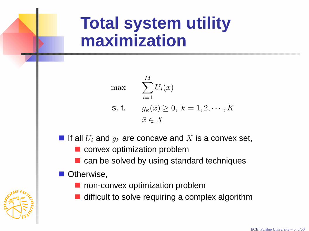
Total system utilitymaximization
max
M∑
i=1
Ui(x̄)
s. t. gk(x̄) ≥ 0, k = 1, 2, · · · , K
x̄ ∈ X
If all Ui and gk are concave and X is a convex set,convex optimization problemcan be solved by using standard techniques
Otherwise,non-convex optimization problemdifficult to solve requiring a complex algorithm
ECE, Purdue University – p. 5/50
Non-convexity inresource allocation
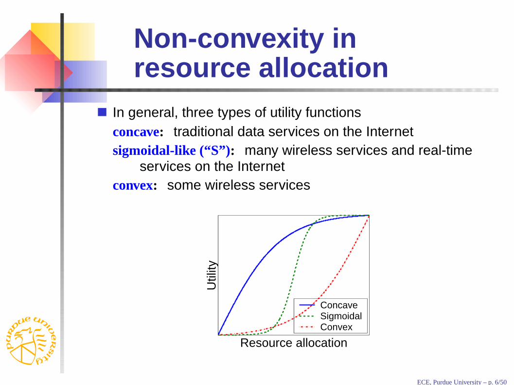
In general, three types of utility functionsconcave: traditional data services on the Internetsigmoidal-like (“S”): many wireless services and real-time
services on the Internetconvex: some wireless services
Resource allocation
Util
ity
ConcaveSigmoidalConvex
ECE, Purdue University – p. 6/50
Non-convexity (cont’d)
0 200
1
γ
f(γ)
BPSKDPSKFSK
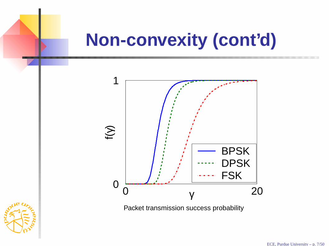
Packet transmission success probability
ECE, Purdue University – p. 7/50
Non-convexity (cont’d)
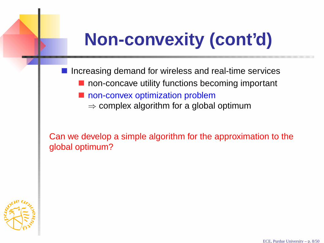
Increasing demand for wireless and real-time servicesnon-concave utility functions becoming importantnon-convex optimization problem⇒ complex algorithm for a global optimum
Can we develop a simple algorithm for the approximation to theglobal optimum?
ECE, Purdue University – p. 8/50

Inefficiency of naiveapproach
11 users and 10 units of a resource
Utility function for each user: U(x)
Approximate U(x) with concave function V (x)
With V (x), for each user,x∗ = 10
11
however, U(x∗) = 0
zero total system utility
By allocating one unit to 10users and zero to one user:
10 units of total systemutility 0 1 2
1
U(x)V(x)
x*
Need resource allocation algorithms taking into account theproperties of non-concave functions
ECE, Purdue University – p. 9/50

Dual approach
Primal problem
max
M∑
i=1
Ui(x̄)
s. t. gk(x̄) ≥ 0,
k = 1, 2, · · · , K
x̄ ∈ X
⇒
⇐
Dual problem
min Q(λ̄)
s. t. λ̄ ≥ 0̄,
Q(λ̄) = maxx̄∈X
{M∑
i=1
Ui(x̄) +K
∑
k=1
λkgk(x̄)}
convex optimization convex optimization
simpler constraints
smaller dimension
In many cases, the dual is easier to solve than the primal
ECE, Purdue University – p. 10/50

Dual approach (cont’d)
Primal problem
max
M∑
i=1
Ui(x̄)
s. t. gk(x̄) ≥ 0,
k = 1, 2, · · · , K
x̄ ∈ X
⇒
6⇐
Dual problem
min Q(λ̄)
s. t. λ̄ ≥ 0̄,
Q(λ̄) = maxx̄∈X
{M∑
i=1
Ui(x̄) +K
∑
k=1
λkgk(x̄)}
non-convex optimiza-tion
convex optimization
simpler constraints
smaller dimension
May not guarantee the feasible and optimal primal solution
ECE, Purdue University – p. 11/50

Part I
Joint power and rate allocation for thedownlink in (CDMA) wireless systems
ECE, Purdue University – p. 12/50
Why joint power and rateallocation?
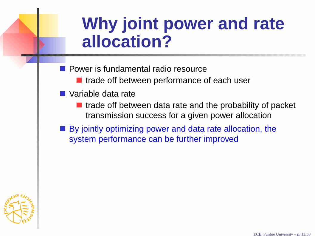
Power is fundamental radio resourcetrade off between performance of each user
Variable data ratetrade off between data rate and the probability of packettransmission success for a given power allocation
By jointly optimizing power and data rate allocation, thesystem performance can be further improved
ECE, Purdue University – p. 13/50
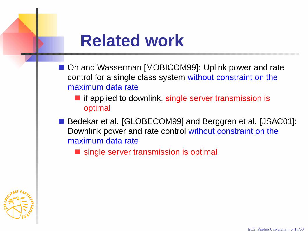
Related workOh and Wasserman [MOBICOM99]: Uplink power and ratecontrol for a single class system without constraint on themaximum data rate
if applied to downlink, single server transmission isoptimal
Bedekar et al. [GLOBECOM99] and Berggren et al. [JSAC01]:Downlink power and rate control without constraint on themaximum data rate
single server transmission is optimal
ECE, Purdue University – p. 14/50

Our workCDMA system that supports variable data rate by variablespreading gain
Downlink in a single cell
Snapshot of a time-slotConstant Path gain and interference level during thetime-slot
Base-station has the total transmission power limit PT
Each user i hasRmax
i : maximum data ratefi: function for packet transmission success probability
ECE, Purdue University – p. 15/50

Signal to Interference andNoise Ratio (SINR)
SINR for user i
γi(Ri, P̄ ) =W
Ri
Pi
θ(∑M
m=1 Pm − Pi) + Ai
M : number of users in the cellW : chip rateθ: orthogonality factorPi: power allocation for user i
Ri: data rate of user i
Ai = Ii/Gi: transmission environment of user i
Ii: background noise and intercell interference at user iGi: path gain from the base-station to user i
SINR is a function of power and rate allocation
ECE, Purdue University – p. 16/50

Packet transmissionsuccess probability: fi
fi is an increasing function of γi
For a given Ri, if∑M
m=1 Pm = PT , fi is
concave function,“S” function, orconvex function
of its own power allocation Pi
0 10
1
P
f(P
)
BPSKDPSKFSK
ECE, Purdue University – p. 17/50
Problem formulation
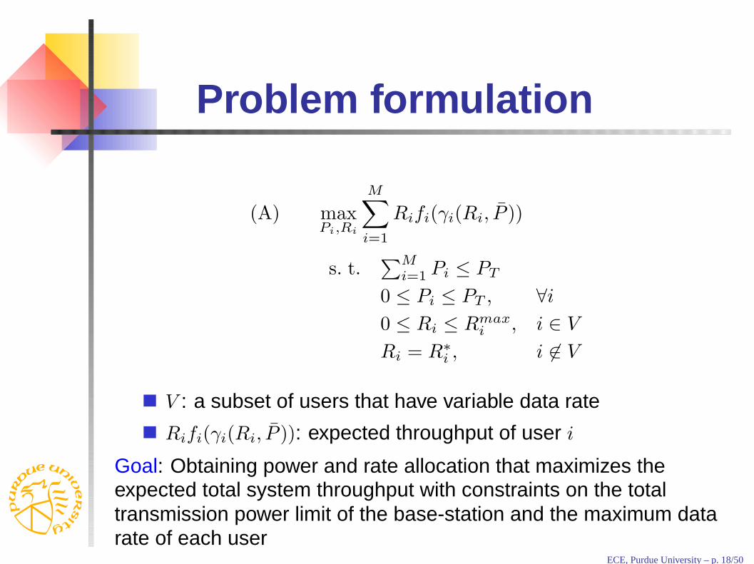
(A) maxPi,Ri
M∑
i=1
Rifi(γi(Ri, P̄ ))
s. t.∑M
i=1 Pi ≤ PT
0 ≤ Pi ≤ PT , ∀i
0 ≤ Ri ≤ Rmaxi , i ∈ V
Ri = R∗i , i 6∈ V
V : a subset of users that have variable data rate
Rifi(γi(Ri, P̄ )): expected throughput of user i
Goal: Obtaining power and rate allocation that maximizes theexpected total system throughput with constraints on the totaltransmission power limit of the base-station and the maximum datarate of each user
ECE, Purdue University – p. 18/50
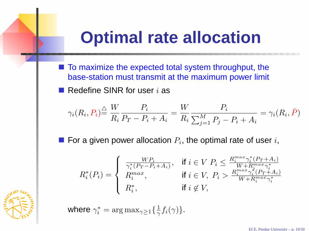
Optimal rate allocation
To maximize the expected total system throughput, thebase-station must transmit at the maximum power limit
Redefine SINR for user i as
γi(Ri, Pi)4=
W
Ri
Pi
PT − Pi + Ai
=W
Ri
Pi∑M
j=1 Pj − Pi + Ai
= γi(Ri, P̄ )
For a given power allocation Pi, the optimal rate of user i,
R∗i (Pi) =
WPi
γ∗i(PT −Pi+Ai)
, if i ∈ V Pi ≤Rmax
i γ∗i (PT +Ai)W+Rmax
iγ∗
i
Rmaxi , if i ∈ V, Pi >
Rmaxi γ∗i (PT +Ai)W+Rmax
iγ∗
i
R∗i , if i 6∈ V,
where γ∗i = arg maxγ≥1{
1γfi(γ)}.
ECE, Purdue University – p. 19/50
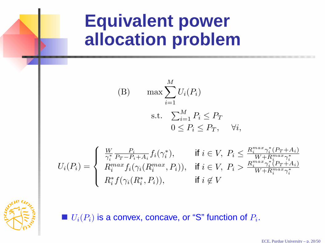
Equivalent powerallocation problem
(B) max
M∑
i=1
Ui(Pi)
s.t.∑M
i=1 Pi ≤ PT
0 ≤ Pi ≤ PT , ∀i,
Ui(Pi) =
Wγ∗
i
Pi
PT −Pi+Aifi(γ
∗i ), if i ∈ V, Pi ≤
Rmaxi γ∗i (PT +Ai)W+Rmax
iγ∗
i
Rmaxi fi(γi(R
maxi , Pi)), if i ∈ V, Pi >
Rmaxi γ∗i (PT +Ai)W+Rmax
iγ∗
i
R∗i f(γi(R
∗i , Pi)), if i 6∈ V
Ui(Pi) is a convex, concave, or “S” function of Pi.
ECE, Purdue University – p. 20/50

Power allocationAmount of power maximizing net utility
Pi(λ) = argmax0≤Pi≤PT
{Ui(Pi) − λPi}
Maximum willingness to pay per unit power
λmaxi = min{λ ≥ 0 | max
0≤P≤PT
{Ui(P ) − λP} = 0}, ∀i
unique for each user i
if λ > λmaxi , then Pi(λ) = 0
if λ < λmaxi , then Pi(λ) > 0
ECE, Purdue University – p. 21/50
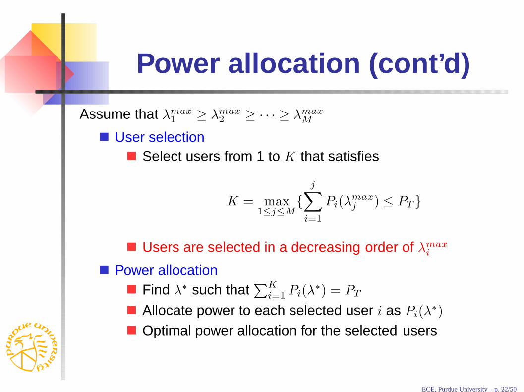
Power allocation (cont’d)
Assume that λmax1 ≥ λmax
2 ≥ · · · ≥ λmaxM
User selectionSelect users from 1 to K that satisfies
K = max1≤j≤M
{
j∑
i=1
Pi(λmaxj ) ≤ PT }
Users are selected in a decreasing order of λmaxi
Power allocationFind λ∗ such that
∑Ki=1 Pi(λ
∗) = PT
Allocate power to each selected user i as Pi(λ∗)
Optimal power allocation for the selected users
ECE, Purdue University – p. 22/50
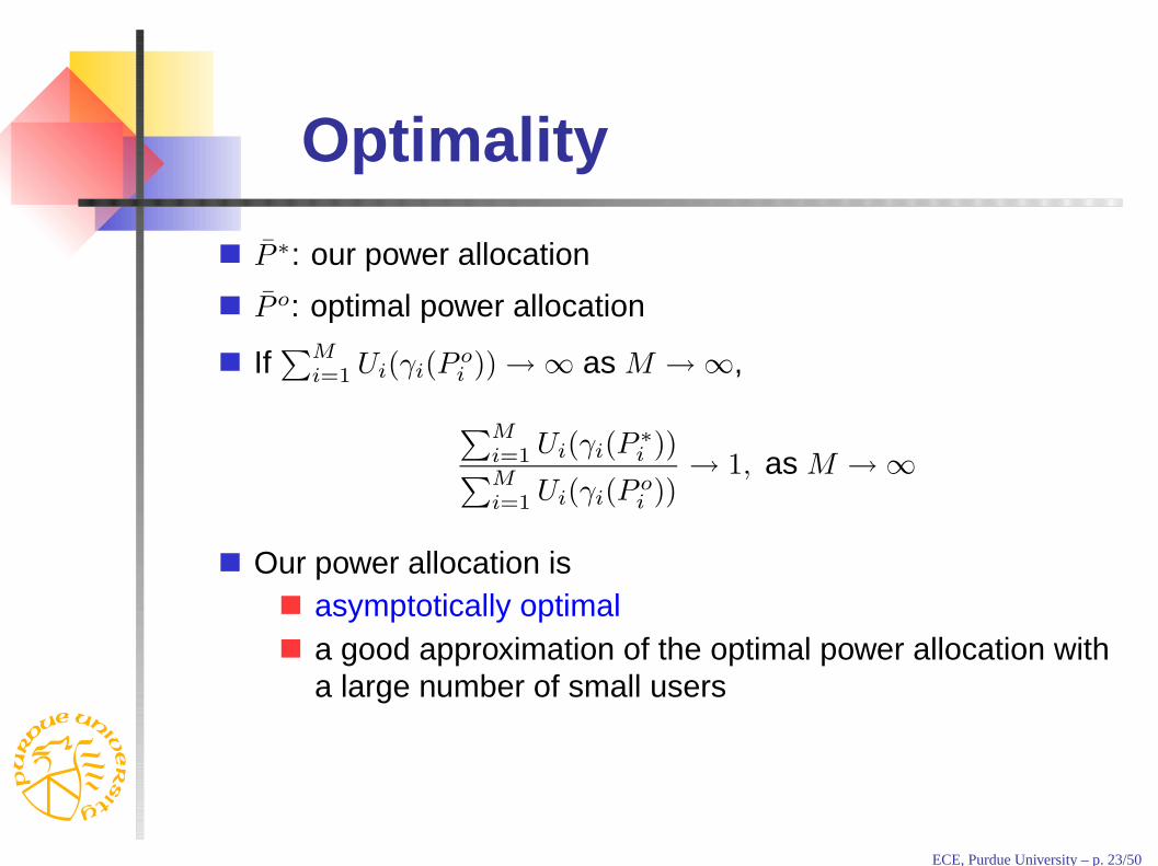
Optimality
P̄ ∗: our power allocation
P̄ o: optimal power allocation
If∑M
i=1 Ui(γi(Poi )) → ∞ as M → ∞,
∑Mi=1 Ui(γi(P
∗i ))
∑Mi=1 Ui(γi(P o
i ))→ 1, as M → ∞
Our power allocation isasymptotically optimala good approximation of the optimal power allocation witha large number of small users
ECE, Purdue University – p. 23/50
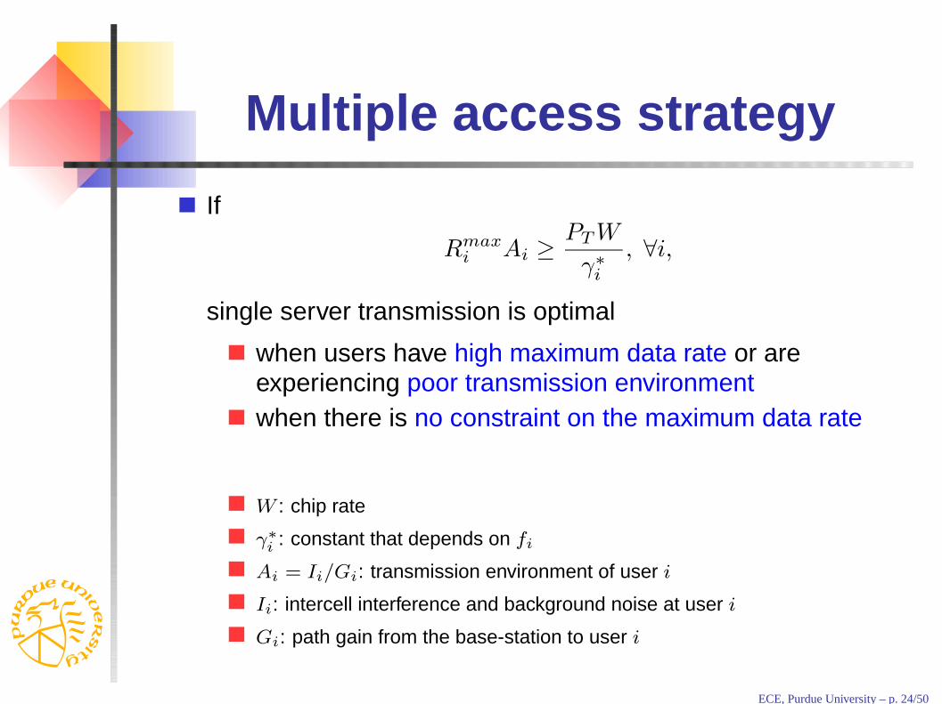
Multiple access strategy
If
Rmaxi Ai ≥
PT W
γ∗i
, ∀i,
single server transmission is optimal
when users have high maximum data rate or areexperiencing poor transmission environmentwhen there is no constraint on the maximum data rate
W : chip rate
γ∗
i: constant that depends on fi
Ai = Ii/Gi: transmission environment of user i
Ii: intercell interference and background noise at user i
Gi: path gain from the base-station to user i
ECE, Purdue University – p. 24/50
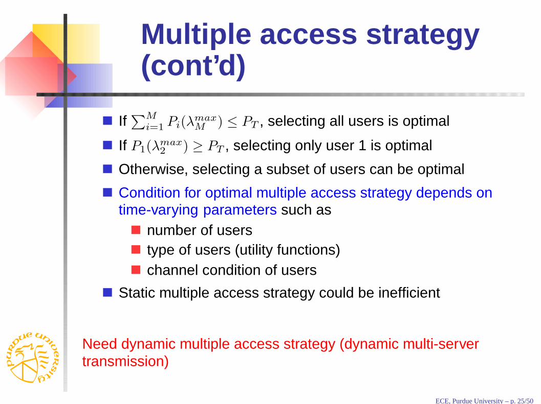
Multiple access strategy(cont’d)
If∑M
i=1 Pi(λmaxM ) ≤ PT , selecting all users is optimal
If P1(λmax2 ) ≥ PT , selecting only user 1 is optimal
Otherwise, selecting a subset of users can be optimal
Condition for optimal multiple access strategy depends ontime-varying parameters such as
number of userstype of users (utility functions)channel condition of users
Static multiple access strategy could be inefficient
Need dynamic multiple access strategy (dynamic multi-servertransmission)
ECE, Purdue University – p. 25/50

User selection strategy
If all users are homogeneous, selecting users according totransmission environment is optimal
higher priority to a user in a better transmissionenvironment
However, if users are heterogeneous, no simple optimal userselection strategy
Our user selection strategy provides a simple and unifiedselection strategy for heterogeneous users
ECE, Purdue University – p. 26/50
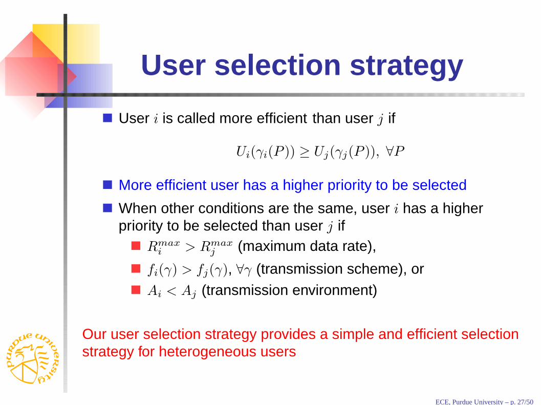
User selection strategy
User i is called more efficient than user j if
Ui(γi(P )) ≥ Uj(γj(P )), ∀P
More efficient user has a higher priority to be selected
When other conditions are the same, user i has a higherpriority to be selected than user j if
Rmaxi > Rmax
j (maximum data rate),
fi(γ) > fj(γ), ∀γ (transmission scheme), or
Ai < Aj (transmission environment)
Our user selection strategy provides a simple and efficient selectionstrategy for heterogeneous users
ECE, Purdue University – p. 27/50

Numerical resultsModel path gain considering distance loss and log-normallydistributed slow shadowing
Two classes of users, for a user in class i,
fi(γ) = ci{1
1 + e−ai(γ−bi)− di}
Compare with the single-server system
BS BS
BS BS BS
BSBSBS
BS
ECE, Purdue University – p. 28/50
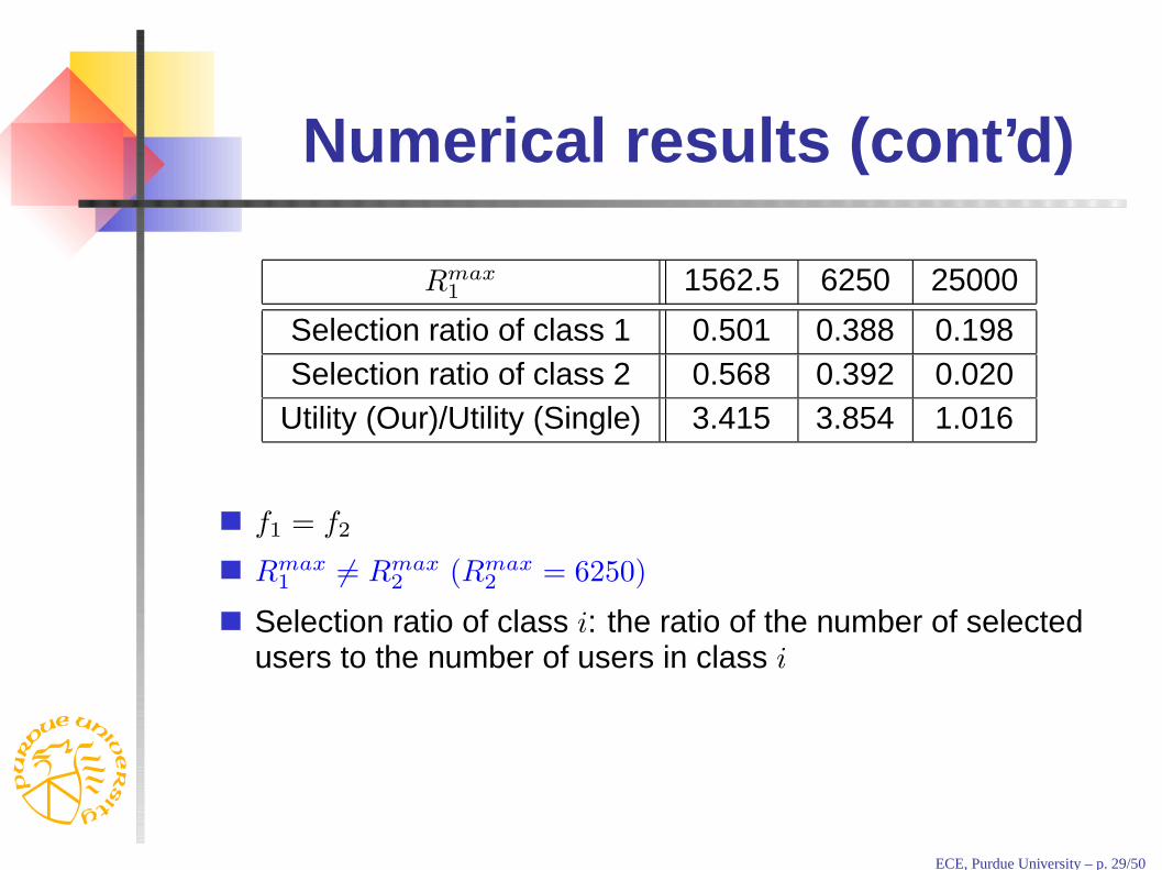
Numerical results (cont’d)
Rmax1 1562.5 6250 25000
Selection ratio of class 1 0.501 0.388 0.198Selection ratio of class 2 0.568 0.392 0.020
Utility (Our)/Utility (Single) 3.415 3.854 1.016
f1 = f2
Rmax1 6= Rmax
2 (Rmax2 = 6250)
Selection ratio of class i: the ratio of the number of selectedusers to the number of users in class i
ECE, Purdue University – p. 29/50
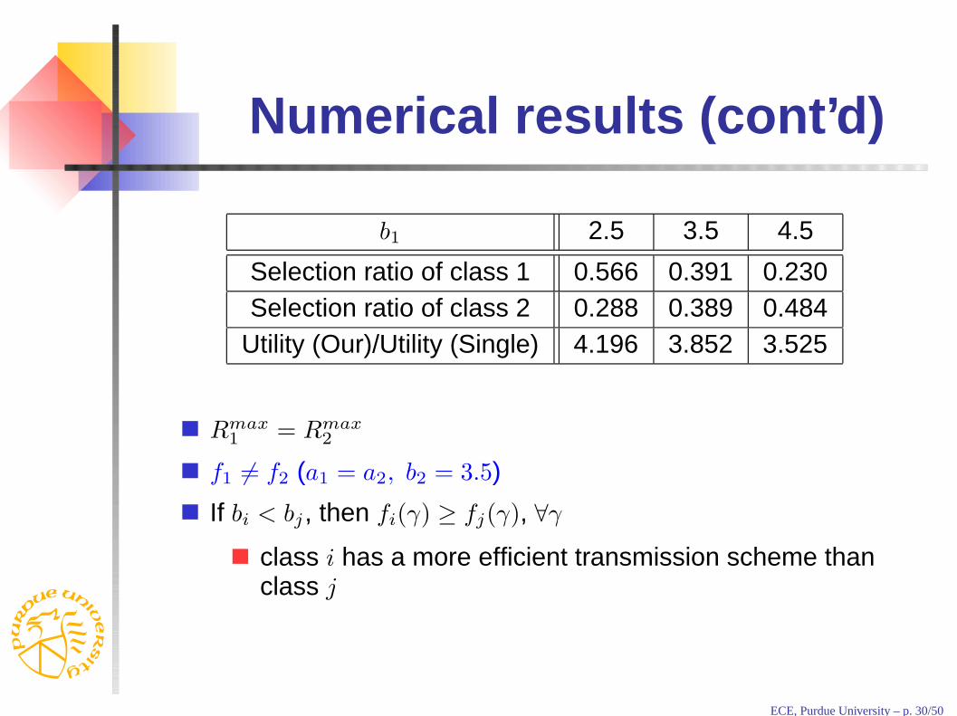
Numerical results (cont’d)
b1 2.5 3.5 4.5
Selection ratio of class 1 0.566 0.391 0.230Selection ratio of class 2 0.288 0.389 0.484
Utility (Our)/Utility (Single) 4.196 3.852 3.525
Rmax1 = Rmax
2
f1 6= f2 (a1 = a2, b2 = 3.5)
If bi < bj , then fi(γ) ≥ fj(γ), ∀γ
class i has a more efficient transmission scheme thanclass j
ECE, Purdue University – p. 30/50
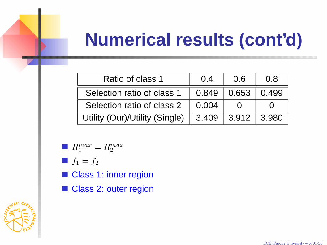
Numerical results (cont’d)
Ratio of class 1 0.4 0.6 0.8
Selection ratio of class 1 0.849 0.653 0.499Selection ratio of class 2 0.004 0 0
Utility (Our)/Utility (Single) 3.409 3.912 3.980
Rmax1 = Rmax
2
f1 = f2
Class 1: inner region
Class 2: outer region
ECE, Purdue University – p. 31/50

Part II
Opportunistic power scheduling for thedownlink in multi-server wireless
systems
ECE, Purdue University – p. 32/50
Why opportunisticscheduling?
Trade-off between efficiency and fairness due tomulti-class userstime-varying and location-dependent channel condition
Our previous problemhigh system efficiencyhowever, unfair to some (inefficient) users
Fairnessachieved by an appropriate scheduling scheme
Opportunistic scheduling considering each user’sdelay tolerancefairness or performance constrainttime-varying channel condition
ECE, Purdue University – p. 33/50
Single-server vs.Multi-server
Single-server schedulingOnly one user can be scheduled in a time-slotIn every time-slot, must decide
which user must be selected
Multi-server schedulingMultiple users can be scheduled in a time-slotIn every time-slot, must decide
how many and which users must be selectedhow much power is allocated to each selected user
Most work studied single-server scheduling
However, single-server scheduling can be inefficientNeed dynamic multi-server scheduling
ECE, Purdue University – p. 34/50
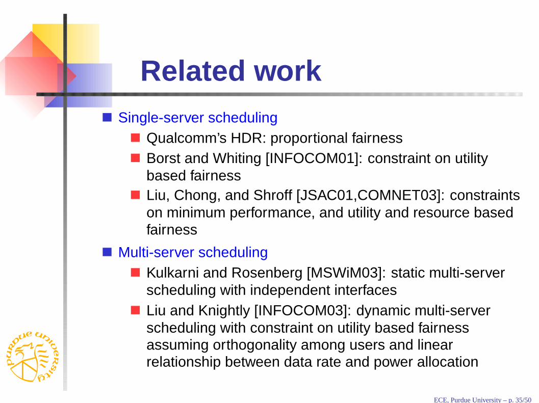
Related workSingle-server scheduling
Qualcomm’s HDR: proportional fairnessBorst and Whiting [INFOCOM01]: constraint on utilitybased fairnessLiu, Chong, and Shroff [JSAC01,COMNET03]: constraintson minimum performance, and utility and resource basedfairness
Multi-server schedulingKulkarni and Rosenberg [MSWiM03]: static multi-serverscheduling with independent interfacesLiu and Knightly [INFOCOM03]: dynamic multi-serverscheduling with constraint on utility based fairnessassuming orthogonality among users and linearrelationship between data rate and power allocation
ECE, Purdue University – p. 35/50
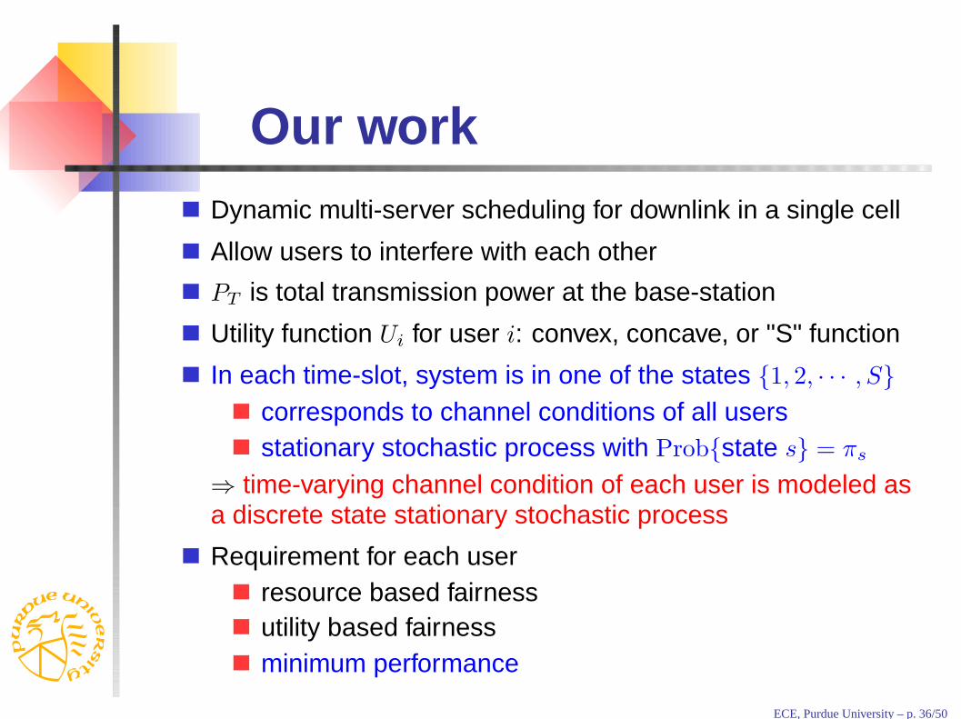
Our workDynamic multi-server scheduling for downlink in a single cell
Allow users to interfere with each other
PT is total transmission power at the base-station
Utility function Ui for user i: convex, concave, or "S" function
In each time-slot, system is in one of the states {1, 2, · · · , S}
corresponds to channel conditions of all usersstationary stochastic process with Prob{state s} = πs
⇒ time-varying channel condition of each user is modeled asa discrete state stationary stochastic process
Requirement for each userresource based fairnessutility based fairnessminimum performance
ECE, Purdue University – p. 36/50

SINR and utility function
SINR for user i when system is in state s
γs,i(Ps,i) =NiPs,i
θ(PT − Ps,i) + As,i
Define
Us,i(Ps,i)4= Ui(γs,i(Ps,i))
The utility function varies randomly according to thechannel condition
ECE, Purdue University – p. 37/50

Problem formulation withminimum performance
(C) maxPs,i
M∑
i=1
E{Ui}(=
M∑
i=1
S∑
s=1
πsUs,i(Ps,i))
s. t. E{Ui}(=
S∑
s=1
πsUs,i(Ps,i)) ≥ Ci, i = 1, 2, · · · , M
M∑
i=1
Ps,i ≤ PT , s = 1, 2, · · · , S
0 ≤ Ps,i ≤ PT , ∀s, i
Goal: Obtaining power scheduling that maximizes the expected totalsystem utility with constraints on the minimum expected utility foreach user and the total transmission power limit for the base-station
ECE, Purdue University – p. 38/50

Problem with minimumperformance (cont’d)
Main difficulties
Feasibilityassume that the system has call admission controlensuring a feasible solution
Non-convexitydual approach
No knowledge for the underlying probability distribution a prioristochastic subgradient algorithm
ECE, Purdue University – p. 39/50

Power scheduling
In each time-slot n, power is allocated to users by solving the dual of
(E) max
M∑
i=1
Ump
s(n),i(µ̄(n), Ps(n),i)
s. t.M∑
i=1
Ps(n),i ≤ PT
0 ≤ Ps(n),i ≤ PT , i = 1, 2, · · · , M
Ump
s(n),i(µ̄(n), Ps(n),i)
4= (1 + µ
(n)i )Us(n),i(Ps(n),i)
Similar to our previous problem
ECE, Purdue University – p. 40/50
Power scheduling(Cont’d)
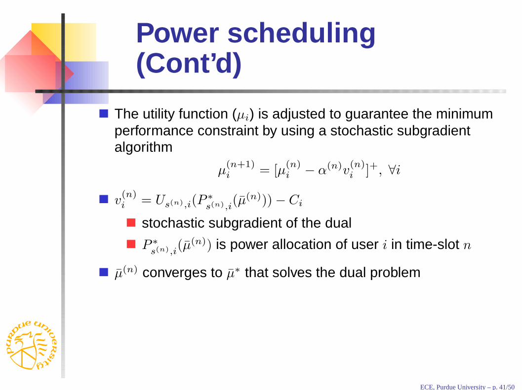
The utility function (µi) is adjusted to guarantee the minimumperformance constraint by using a stochastic subgradientalgorithm
µ(n+1)i = [µ
(n)i − α(n)v
(n)i ]+, ∀i
v(n)i = Us(n),i(P
∗s(n),i
(µ̄(n))) − Ci
stochastic subgradient of the dual
P ∗s(n),i
(µ̄(n)) is power allocation of user i in time-slot n
µ̄(n) converges to µ̄∗ that solves the dual problem
ECE, Purdue University – p. 41/50
Feasibility
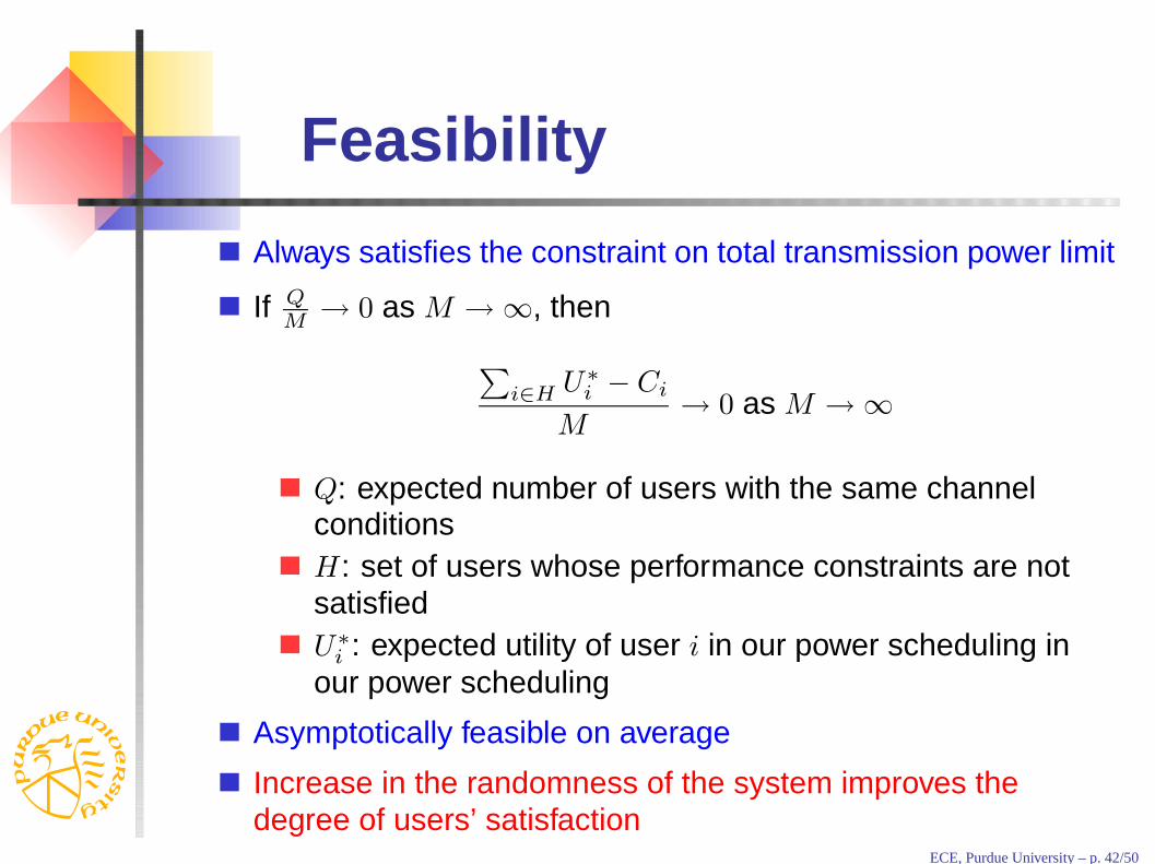
Always satisfies the constraint on total transmission power limit
If QM
→ 0 as M → ∞, then
∑
i∈H U∗i − Ci
M→ 0 as M → ∞
Q: expected number of users with the same channelconditionsH: set of users whose performance constraints are notsatisfiedU∗
i : expected utility of user i in our power scheduling inour power scheduling
Asymptotically feasible on average
Increase in the randomness of the system improves thedegree of users’ satisfaction
ECE, Purdue University – p. 42/50
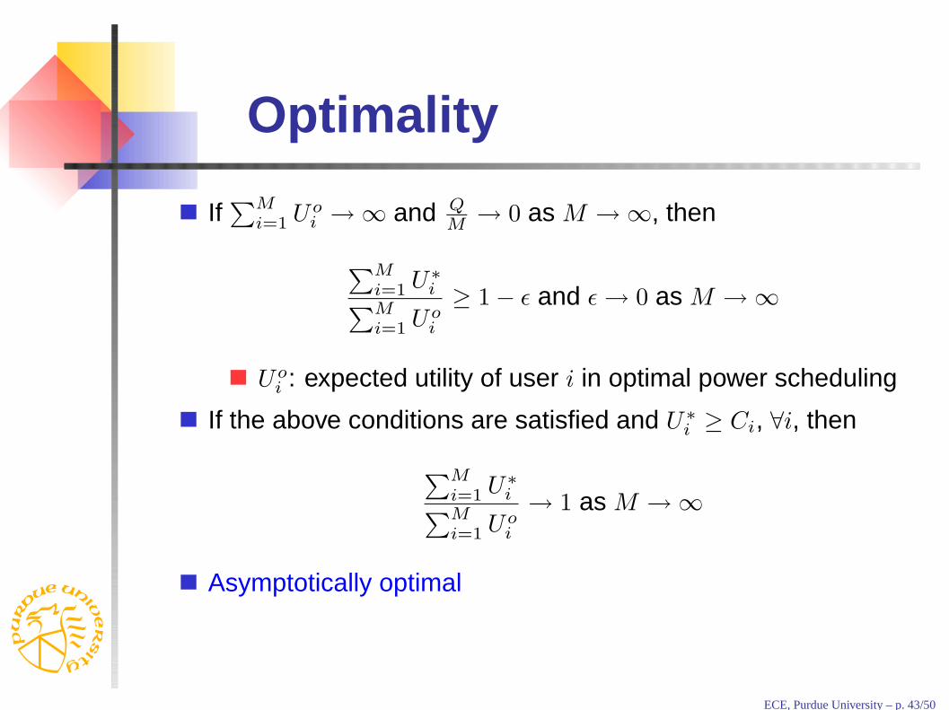
Optimality
If∑M
i=1 Uoi → ∞ and Q
M→ 0 as M → ∞, then
∑Mi=1 U∗
i∑M
i=1 Uoi
≥ 1 − ε and ε → 0 as M → ∞
Uoi : expected utility of user i in optimal power scheduling
If the above conditions are satisfied and U∗i ≥ Ci, ∀i, then
∑Mi=1 U∗
i∑M
i=1 Uoi
→ 1 as M → ∞
Asymptotically optimal
ECE, Purdue University – p. 43/50

Numerical resultsThe same cellular model as our previous problem
Four users and each user i
same sigmoid utility function Ui (Ui(0) = 0 and Ui(∞) = 1)same performance constraint Ci = 0.59
distance from the base-station to user i: di
d1 < d2 < d3 < d4
Performance comparison withNon-opportunistic schedulingGreedy scheduling
ECE, Purdue University – p. 44/50
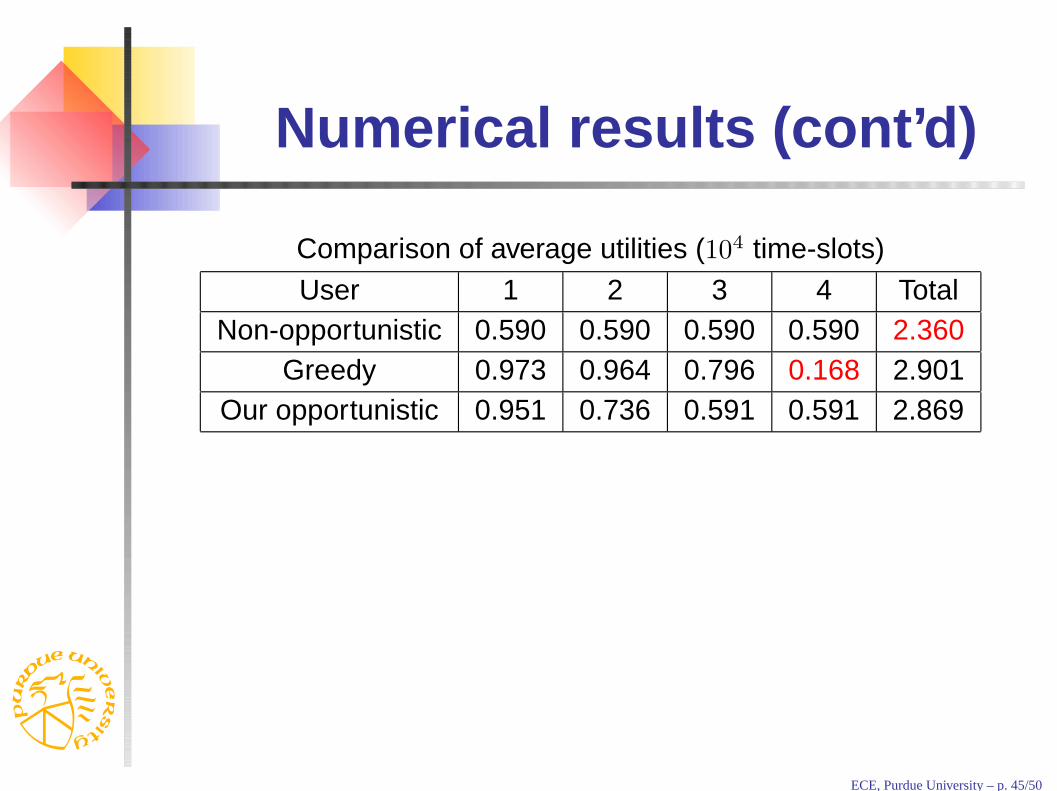
Numerical results (cont’d)
Comparison of average utilities (104 time-slots)
User 1 2 3 4 TotalNon-opportunistic 0.590 0.590 0.590 0.590 2.360
Greedy 0.973 0.964 0.796 0.168 2.901Our opportunistic 0.951 0.736 0.591 0.591 2.869
ECE, Purdue University – p. 45/50
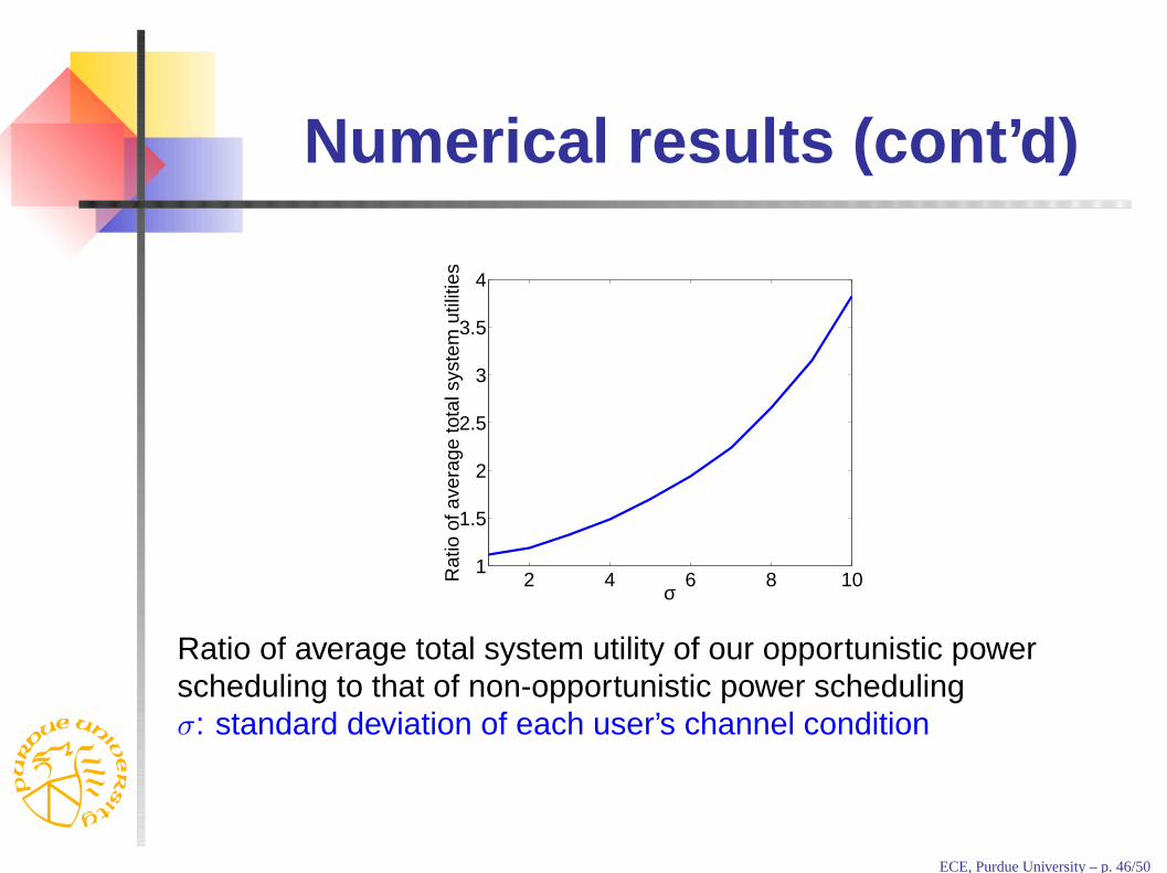
Numerical results (cont’d)
2 4 6 8 101
1.5
2
2.5
3
3.5
4
σ
Rat
io o
f ave
rage
tota
l sys
tem
util
ities
Ratio of average total system utility of our opportunistic powerscheduling to that of non-opportunistic power schedulingσ: standard deviation of each user’s channel condition
ECE, Purdue University – p. 46/50

ConclusionUtility framework
suitable for resource allocation with multi-media and dataservicesa useful tool for resource allocation in the nextgenerations of communication networksnon-convex optimization problems in many cases
Dual approach providesefficient solution in many casessimple algorithm that can be easily implemented with a(distributed) network protocol
ECE, Purdue University – p. 47/50

Conclusion (cont’d)
In wireless systems
Single server transmission is optimal only when all users havehigh data rate
In general, need dynamic multiple access (dynamicmulti-server system)
Trade-off between efficiency and fairnessOpportunistic scheduling achieves both of them
Randomness of the system could be beneficial to efficient andfair resource allocation, if appropriately exploited
ECE, Purdue University – p. 48/50

Conclusion (cont’d)
Other problems
Pricing based base-station assignmentconsiders both transmission environment of the user andcongestion level of the base-station
Congestion control on the Internetalgorithms for concave utility functions cause instabilityand congestion in the presence of real-time services withnon-concave utility functionsself-regulating property stabilizes the system andalleviates congestion
ECE, Purdue University – p. 49/50

Future workScheduling considering
user dynamicsnon-stationary environmentdelay or short-term fairness constraints
Resource allocation considering upper layer protocols (e.g.,TCP)
Resource allocation for uplink and multi-cellular system
ECE, Purdue University – p. 50/50