5. Smooth convex optimization

Lecture 5

Smooth convex minimizationproblems

To the moment we have more or less complete impression of what is the complexity ofsolving general nonsmooth convex optimization problems and what are the correspondingoptimal methods. In this lecture we treat a new topic: optimal methods for smooth convexminimization. We shall start with the simplest case of unconstrained problems with smoothconvex objective. Thus, we shall be interested in methods for solving the problem

(f) minimize f(x) over x ∈ Rn,

where f is a convex function of the smootness type C1,1, i.e., a continuously differentiablewith Lipschitz continuous gradient:

|f ′(x)− f ′(y)| ≤ L(f)|x− y| ∀x, y ∈ Rn;

from now on | · | denotes the standard Euclidean norm. We assume also that the problem issolvable (i.e., Argmin f 6= ∅) and denote by R(f) the distance from the origin (which will bethe starting point for the below methods) to the optimal set of (f). Thus, we have definedcertain family Sn of convex minimization problems; the family is comprised of all programs(f) associated with C1,1-smooth convex functions f on Rn which are below bounded andattain their minimum. As usual, we provide the family with the first-order oracle O which,given on input a point x ∈ Rn, reports the value f(x) and the gradient f ′(x) of the objectiveat the point. The accuracy measure we are interested in is the absolute inaccuracy in termsof the objective:

ε(f, x) = f(x)−minRn

f.

It turns out that complexity of solving a problem from the above family heavily depends onthe Lipschitz constant L(f) of the objective and the distance R(f) from the starting pointto the optimal set; this is why in order to analyse complexity it makes sense to speak noton the whole family Sn, but on its subfamilies

Sn(L,R) = {f ∈ S | L(f) ≤ L,R(f) ≤ R},

where L and R are positive parameters identifying, along with n, the subfamily.

109

110 LECTURE 5. SMOOTH CONVEX MINIMIZATION PROBLEMS

5.1 Traditional methods

Unconstrained minimization of C1,1-smooth convex functions is, in a sense, the most tradi-tional area in Nonlinear Programming. There are many methods for these problems: thesimplest Gradient Descent method with constant stepsize, Gradient Descent with completerelaxation, numerous Conjugate Gradent routines, etc. Note that I did not mention theNewton method, since the method, in its basic form, requires twice continuously differen-tiable objectives and second-order information, and we are speaking about the first-orderinformation and objectives which are not necessarily twice continuously differentiable. Onemight think that since the field is so well-studied, among the traditional methods there forsure are optimal ones; surprisingly, this is not the case, as we shall see in a while.

To get a kind of a reference point, let me start with the simplest method for smoothconvex minimization - the Gradient Descent. This method, as applied to (f), generates thesequence of search points

xi+1 = xi − γif ′(xi), x0 = 0. (5.1.1)

Here γi are positive stepsizes; various versions of the Gradient Descent differ from each otherby the rules for choosing these stepsizes. In the simplest version - Gradient Descent withconstant stepsize - one sets

γi ≡ γ. (5.1.2)

With this rule for stepsizes the convergence of the method is ensured if

0 < γ <2

L(f). (5.1.3)

Proposition 5.1.1 Under assumption (5.1.3) process (5.1.1) - (5.1.2) converges at the rateO(1/N): for all N ≥ 1 one has

f(xN)−min f ≤ R2(f)

γ(2− γL(f))N−1. (5.1.4)

In particular, with the optimal choice of γ, i.e., γ = L−1(f), one has

f(xN)−min f ≤ L(f)R2(f)

N. (5.1.5)

Proof. Let x∗ be the minimizer of f of the norm R(f). We have

f(x) + hTf ′(x) ≤ f(x+ h) ≤ f(x) + hTf ′(x) +L(f)

2|h|2. (5.1.6)

Here the first inequality is due to the convexity of f and the second one – to the Lipschitzcontinuity of the gradient of f . Indeed,

f(y)− f(x)− (y − x)Tf ′(x) = (y − x)T∫ 1

0[f ′(x− t(y − x))− f ′(x)]dt

≤ |y − x|2L(f)∫ 1

0tdt =

L(f)

2|y − x|2

5.1. TRADITIONAL METHODS 111

From the second inequality of (5.1.6) it follows that

f(xi+1) ≤ f(xi)− γ|f ′(xi)|2 +L(f)

2γ2|f ′(xi)|2 =

= f(xi)− ω|f ′(xi)|2, ω = γ(1− γL(f)/2) > 0, (5.1.7)

whence

|f ′(xi)|2 ≤ ω−1(f(xi)− f(xi+1)); (5.1.8)

we see that the method is monotone and that

∑i

|f ′(xi)|2 ≤ ω−1(f(x1)− f(x∗)) = ω−1(f(0)− f(x∗)) ≤ ω−1L(f)R2(f)

2(5.1.9)

(the concluding inequality follows from the second inequality in (5.1.6), where one shouldset x = x∗, h = −x∗).

We have

|xi+1 − x∗|2 = |xi − x∗|2 − 2γ(xi − x∗)Tf ′(xi) + γ2|f ′(xi)|2 ≤

≤ |xi − x∗|2 − 2γ(f(xi)− f(x∗)) + γ2|f ′(xi)|2

(we have used convexity of f , i.e., have applied the first inequality in (5.1.6) with x = xi,h = x∗ − xi). Taking sum of these inequalities over i = 1, ..., N and taking into account(5.1.9), we come to

N∑i=1

(f(xi)− f(x∗)) ≤ (2γ)−1R2(f) + γω−1L(f)R2(f)/4 =R2(f)

γ(2− γL(f)).

Since the absolute inaccuracies εi = f(xi)− f(x∗), as we already know, decrease with i, weobtain from the latter inequality

εN ≤R2(f)

γ(2− γL(f))N−1,

as required.

In fact our upper bound on the accuracy of the Gradient Descent is sharp: it is easilyseen that, given L > 0, R > 0, a positive integer N and a stepsize γ > 0, one can point outa quadratic form f(x) on the plane such that L(f) = L, R(f) = R and for the N -th pointgenerated by the Gradient Descent as applied to f one has

f(xN)−min f ≥ O(1)LR2

N.


5.2 Complexity of classes Sn(L,R)The rate of convergence of the Gradient Descent O(N−1) given by Proposition 5.1.1 isdimension-independent and is twice better in order than the known to us optimal in thenonsmooth large scale case rate O(N−1/2). There is no surprise in the progress: we havepassed from a very wide family of nonsmooth convex problems to the much more narrowfamily of smooth convex problems. What actually is a surprise is that the rate O(N−1) stillis not optimal; the optimal dimension-independent rate of convergence in smooth convexminimization turns out to be O(N−2).

Theorem 5.2.1 The complexity of the family Sn(L,R) satisfies the bounds

O(1) min

n,√LR2

ε

≤ Compl(ε) ≤c√

4LR2

εb (5.2.10)

with positive absolute constant O(1).

Note that in the large scale case, namely, when

n2 ≥ LR2

ε,

the upper complexity bound only by absolute constant factor differs from the lower one.When dimension is not so large, namely, when

n2 <<LR2

ε,

both lower and upper complexity bounds are not sharp; the lower bound does not say any-thing reasonable, and the upper is valid, but significantly overestimates the complexity. Infact in this ”low scale” case the complexity turns out to be O(1)n ln(LR2/ε), i.e., is basicallythe same as for nonsmooth convex problems. Roughly speaking, in a fixed dimension theadvantages of smoothness can be exploited only when the required accuracy is not too high.

Let us prove the theorem. As always, we should point out a method associated with theupper complexity bound and to prove somehow the lower bound.

5.2.1 Upper complexity bound: Nesterov’s method

The upper complexity bound is associated with a relatively new construction developed byYurii Nesterov in 1983. This construction is a very nice example which demonstrates themeaning of the complexity approach; the method with the rate of convergence O(N−2) wasfound mainly because the investigating of complexity enforced the belief that such a methodshould exist.

The method, as applied to problem (f), generates the sequence of search points xi,i = 0, 1, ..., and the sequence of approximate solutions yi, i = 1, 2, ..., along with auxiliarysequences of vectors qi, positive reals Li and reals ti ≥ 1, according to the following rules:

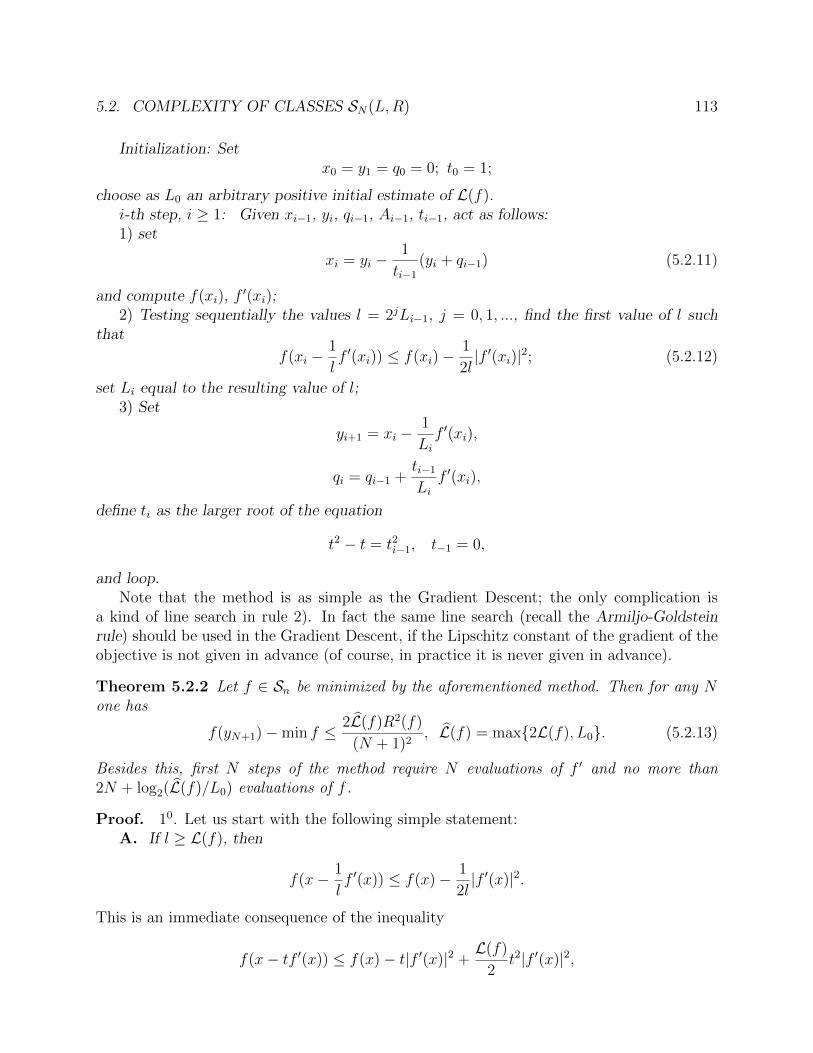
5.2. COMPLEXITY OF CLASSES SN(L,R) 113

Initialization: Setx0 = y1 = q0 = 0; t0 = 1;

choose as L0 an arbitrary positive initial estimate of L(f).i-th step, i ≥ 1: Given xi−1, yi, qi−1, Ai−1, ti−1, act as follows:1) set

xi = yi −1

ti−1

(yi + qi−1) (5.2.11)

and compute f(xi), f′(xi);

2) Testing sequentially the values l = 2jLi−1, j = 0, 1, ..., find the first value of l suchthat

f(xi −1

lf ′(xi)) ≤ f(xi)−

1

2l|f ′(xi)|2; (5.2.12)

set Li equal to the resulting value of l;3) Set

yi+1 = xi −1

Lif ′(xi),

qi = qi−1 +ti−1

Lif ′(xi),

define ti as the larger root of the equation

t2 − t = t2i−1, t−1 = 0,

and loop.Note that the method is as simple as the Gradient Descent; the only complication is

a kind of line search in rule 2). In fact the same line search (recall the Armiljo-Goldsteinrule) should be used in the Gradient Descent, if the Lipschitz constant of the gradient of theobjective is not given in advance (of course, in practice it is never given in advance).

Theorem 5.2.2 Let f ∈ Sn be minimized by the aforementioned method. Then for any None has

f(yN+1)−min f ≤ 2L(f)R2(f)

(N + 1)2, L(f) = max{2L(f), L0}. (5.2.13)

Besides this, first N steps of the method require N evaluations of f ′ and no more than2N + log2(L(f)/L0) evaluations of f .

Proof. 10. Let us start with the following simple statement:A. If l ≥ L(f), then

f(x− 1

lf ′(x)) ≤ f(x)− 1

2l|f ′(x)|2.

This is an immediate consequence of the inequality

f(x− tf ′(x)) ≤ f(x)− t|f ′(x)|2 +L(f)

2t2|f ′(x)|2,


which in turn follows from (5.1.6).We see that if L0 ≥ L(f), then all Li are equal to L0, since l = L0 for sure passes all

tests (5.2.12). Further, if L0 < L(f), then the quantities Li never become ≥ 2L(f). Indeed,in the case in question the starting value L0 is ≤ L(f). When updating Li−1 into Li, wesequentially subject to test (5.2.12) the quantities Li−1, 2Li−1, 4Li−1, ..., and choose as Lithe first of these quantities which passes the test. It follows that if we come to Li ≥ 2L(f),then the quantity Li/2 ≥ L(f) did not pass one of our tests, which is impossible by A. Thus,

Li ≤ L(f), i = 1, 2, ...

Now, the total number of evaluations of f ′ in course of the first N steps clearly equalsto N , while the total number of evaluations of f is N plus the total number, K, of tests(5.2.12) performed during these steps. Among K tests there are N successful (when thetested value of l satisfies (5.2.12)), and each of the remaining tests increases value of L·by the factor 2. Since L·, as we know, is ≤ 2L(f), the number of these remaining tests is≤ log2(L(f)/L0), so that the total number of evaluations of f in course of the first N stepsis ≤ 2N + log2(L(f)/L0), as claimed.

20. It remains to prove (5.2.13). To this end let us add to A. the following observationB. For any i ≥ 1 and any y ∈ Rn one has

f(y) ≥ f(yi+1) + (y − xi)Tf ′(xi) +1

2Li|f ′(xi)|2. (5.2.14)

Indeed, we have

f(y) ≥ (y − xi)Tf ′(xi) + f(xi) ≥ (y − xi)Tf ′(xi) +(f(yi+1) +

1

2Li|f ′(xi)|2

)(the concluding inequality follows from A by the definition of yi+1).

30. Let x∗ be the minimizer of f of the norm R(f), and let

εi = f(yi)− f(x∗)

be the absolute accuracy of i-th approximate solution generated by the method.Applying (5.2.14) to y = x∗, we come to inequality

0 ≥ εi+1 + (x∗ − xi)Tf ′(xi) +1

2Li|f ′(xi)|2. (5.2.15)

Now, the relation (5.2.11) can be rewritten as

xi = (ti−1 − 1)(yi − xi)− qi−1,

and with this substitution (5.2.15) becomes

0 ≥ εi+1 + (x∗)Tf ′(xi) + (ti−1 − 1)(xi − yi)Tf ′(xi) + qTi−1f′(xi) +

1

2Li|f ′(xi)|2. (5.2.16)


At the same time, (5.2.14) as applied to y = yi results in

0 ≥ f(yi+1)− f(yi) + (yi − xi)Tf ′(xi) +1

2Li|f ′(xi)|2,

which implies an upper bound on (yi − xi)Tf ′(xi), or, which is the same, a lower bound onthe quantity (xi − yi)Tf ′(xi), namely,

(xi − yi)Tf ′(xi) ≥ εi+1 − εi +1

2Li|f ′(xi)|2.

Substituting this estimate into (5.2.16), we come to

0 ≥ ti−1εi+1 − (ti−1 − 1)εi + (x∗)Tf ′(xi) + qTi−1f′(xi) + ti−1

1

2Li|f ′(xi)|2. (5.2.17)

Multiplying this inequality by ti−1/Li, we come to

0 ≥t2i−1

Liεi+1 −

t2i−1 − ti−1

Liεi + (x∗)T

(ti−1

Lif ′(xi)

)+ qTi−1

ti−1

Lif ′(xi) +

t2i−1

2L2i

|f ′(xi)|2. (5.2.18)

We have (ti−1/Li)f′(xi) = qi − qi−1 and t2i−1 − ti−1 = t2i−2 (here t−1 = 0); thus, (5.2.18) can

be rewritten as

0 ≥t2i−1

Liεi+1 −

t2i−2

Liεi + (x∗)T (qi − qi−1) + qTi−1(qi − qi−1) +

1

2|qi − qi−1|2 =

=t2i−1

Liεi+1 −

t2i−2

Liεi + (x∗)T (qi − qi−1) +

1

2|qi|2 −

1

2|qi−1|2.

Since the quantities Li do not decrease with i and εi+1 is nonnegative, we shall onlystrengthen the resulting inequality by replacing the coefficient t2i−1/Li at εi+1 by t2i−1/Li+1;thus, we come to the inequality

0 ≥t2i−1

Li+1

εi+1 −t2i−2

Liεi + (x∗)T (qi − qi−1) +

1

2|qi|2 −

1

2|qi−1|2.

Taking sum of these inequalities over i = 1, ..., N , we come to

t2N−1

LN+1

εN+1 ≤ −(x∗)T qN −1

2|qN |2 ≤

1

2|x∗|2 ≡ R2(f)/2; (5.2.19)

thus,

εN+1 ≤LN+1R

2(f)

2t2N−1

. (5.2.20)

As we know, LN+1 ≤ L(f), and from the recurrency

ti =1

2(1 +

√1 + 4t2i−1), t0 = 1


it immediately follows that ti ≥ (i+ 1)/2; therefore (5.2.20) implies (5.2.13).Theorem 5.2.2 implies the upper complexity bound announced in (5.2.10); to see this, it

suffices to apply to a problem from Sn(L,R) the Nesterov method with L0 = L; in this case,as we know from A., all Li are equal to L0, so that we may skip the line search 2); thus, torun the method it will be sufficient to evaluate f and f ′ at the search points only, and inview of (5.2.13) to solve the problem within absolute accuracy ε it is sufficient to performthe indicated in (5.2.10) number of oracle calls.

Let me add some words about the Nesterov method. As it is, it looks as an analyticaltrick; I would be happy to present to you a geometrical explanation, but I do not know it.Historically, there were several predecessors of the method with more clear geometry, butthese methods had slightly worse efficiency estimates; the progress in these estimates madethe methods less and less geometrical, and the result is as you just have seen. By the way, Ihave said that I do not know geometrical explanation of the method, but I can immediatelypoint out geometrical presentation of the method. It is easily seen that the vectors qi can beeliminated from the equations describing the method, and the resulting description is simply

xi = (1 + αi)yi − αiyi−1, αi =ti−2 − 1

ti−1

, i ≥ 1, y0 = y1 = 0,

yi+1 = xi −1

Lif ′(xi)

(Li are given by rule 2)). Thus, i-th search point is a kind of forecast - it belongs to theline passing through the pair of the last approximate solutions yi, yi−1, and for large i yi isapproximately the middle of the segment [yi−1, xi]; the new approximate solution is obtainedfrom this forecast xi by the standard Gradient Descent step with Armiljo-Goldstein rule forthe steplength.

Let me make one more remark. As we just have seen, the simplest among the traditionalmethods for smooth convex minimization - the Gradient Descent - is far from being optimal;its worst-case order of convergence can be improved by factor 2. What can be said aboutoptimality of other traditional methods (such as Conjugate Gradients, etc.)? Surprisingly,the answer is as follows: no one of the traditional methods is proved to be optimal, i.e., withthe rate of convergence O(N−2). For some versions of the Conjugate Gradient family it isknown that their worst-case behaviour is not better, and sometimes is even worse, than thatone of the Gradient Descent, and no one of the remaining traditional methods is known tobe better than the Gradient Descent.

5.2.2 Lower bound

Surprisingly, the ”most difficult” smooth convex minimization problems are the quadraticones; the lower complexity bound in (5.2.10) comes exactly from investigating the complexityof large scale unconstrained convex quadratic minimization with respect to the first orderminimization methods (I stress this ”first order”; of course, the second order methods, likethe Newton one, minimize a quadratic function in one step).


Letσ = {σ1 < σ2 < ... < σn}

be a set of n points from the half-interval (0, L] and

µ = {µ1, ..., µn}

be a sequence of nonnegative reals such that

n∑i=1

µi = R2.

Let e1, ..., en be the standard orths in Rn, and let

A = Diag{σ1, ..., σn},

b =n∑i=1

√µiσiei.

Consider the quadratic form

f(x) ≡ fσ,µ(x) =1

2xTAx− xT b;

this function clearly is smooth, with the gradient f ′(x) = Ax being Lipschitz continuouswith constant L; the minimizer of the function is the vector

n∑i=1

√µiei, (5.2.21)

and the norm of this vector is exactly R. Thus, the function f belongs to Sn(L,R). Now,let U be the family of all rotations of Rn which remain the vector b invariant, i.e., the familyof all orthogonal n × n matrices U such that Ub = b. Since Sn(L,R) contains the functionf , it contains also the family F(σ, µ) comprised by all rotations

fU(x) = f(Ux)

of the function f associated with U ∈ U . Note that fU is the quadratic form

1

2xTAUx− xT b, AU = UTAU.

Thus, the family F(σ, µ) is contained in Sn(L,R), and therefore the complexity of this familyunderestimates the complexity of Sn(L,R). What I am going to do is to bound from belowthe complexity of F(σ, µ) and then choose the worst ”parameters” σ and µ to get the bestpossible, within the bounds of this approach, lower bound for the complexity of Sn(L,R).

Consider a convex quadratic form

g(x) =1

2xTQx− xT b;


here Q is a positive semidefinite symmetric n × n matrix. Let us associate with this formthe Krylov subspaces

Ei(g) = Rb+ RQb+ ...+ RQi−1b

and the quantitiesε∗i (g) = min

x∈Ei(Q,b)g(x)− min

x∈Rng(x).

Note that these quantities clearly remain invariant under rotations

(Q, b) 7→ (UTQU,UT b)

associated with n×n orthogonal matrices U . In particular, the quantities ε∗i (fU) associatedwith fU ∈ F(σ, µ) in fact do not depend on U :

ε∗i (fU) ≡ ε∗i (f). (5.2.22)

The key to our complexity estimate is given by the following:

Proposition 5.2.1 Let M be a method for minimizing quadratic functions from F(σ, µ)and M be the complexity of the method on the latter family. Then there is a problem fUin the family such that the result x of the method as applied to fU belongs to the spaceE2M+1(fU); in particular, the inaccuracy of the method on the family in question is at leastε∗2M+1(fU) ≡ ε∗2M+1(f).

The proposition will be proved in the concluding part of the lecture.Let us derive from Proposition 5.2.1 the desired lower complexity bound. Let ε > 0 be

fixed, let M be the complexity Compl(ε) of the family Sn(L,R) associated with this ε. Thenthere exists a method which solves in no more than M steps within accuracy ε all problemsfrom Sn(L,R), and, consequently, all problems from the smaller families F(σ, µ), for all σand µ. According to Proposition 5.2.1, this latter fact implies that

ε∗2M+1(f) ≤ ε (5.2.23)

for any f = fσ,µ. Now, the Krylov space EN(f) is, by definition, comprised of linear com-binations of the vectors b, Ab, ..., AN−1b, or, which is the same, of the vectors of the formq(A)b, where q runs over the space PN of polynomials of degrees ≤ N . Now, the coordinatesof the vector b are σi

√µi, so that the coordinates of q(A)b are q(σi)σi

√µi. Therefore

f(q(A)b) =n∑i=1

{1

2σ3i q

2(σi)µi − σiq(σi)µi}.

As we know, the minimizer of f over Rn is the vector with the coordinates√µi, and the

minimal value of f , as it is immediately seen, is

−1

2

n∑i=1

σiµi.


We come to

2ε∗N(f) = minq∈PN−1

n∑i=1

{σ3i q

2(σi)µi − 2σiq(σi)µi}+n∑i=1

σiµi =

= minq∈PN−1

n∑i=1

σi(1− σiq(σi))2µi.

Substituting N = 2M + 1 and taking in account (5.2.23), we come to

2ε ≥ minq∈P2M

n∑i=1

σi(1− σiq(σi))2µi. (5.2.24)

This inequality is valid for all sets σ = {σi}ni=1 comprised of n different points from (0, L]and all sequences µ = {µi}ni=1 of nonnegative reals with the sum equal to R2; it follows that

2ε ≥ supσ

maxµ

minp∈P2M

n∑i=1

σi(1− σiq(σi))2µi; (5.2.25)

due to the von Neumann Lemma, one can interchange here the minimization in q and themaximization in µ, which immediately results in

2ε ≥ R2 supσ

minq∈P2M

maxσ∈σ

σ(1− σq(σ))2. (5.2.26)

Now, the quantityν2(σ) = min

q∈P2M

maxσ∈σ

σ(1− σq(σ))2

is nothing but the squared best quality of the approximation, in the uniform (Tschebyshev’s)norm on the set σ, of the function

√σ by a linear combination of the 2M functions

φi(σ) = σi+1/2, i = 0, ..., 2M − 1

We have the following result (its proof is the subject of the exercises to this lecture):the quality of the best uniform on the segment [0, L] approximation of the function

√σ

by a linear combination of 2M functions φi(σ) is the same as the quality of the best uniformapproximation of the function by such a linear combination on certain (2M+1)-point subsetof [0, L].

We see that if 2M + 1 ≤ n, then

2ε ≥ R2 supσν2(σ) = R2 min

q∈P2M

maxσ∈[0,L]

σq2(σ).

The concluding quantity in this chain can be computed explicitly; it is equal to (4M +1)−2LR2. Thus, we have established the implication

2M + 1 ≤ n⇒ (4M + 1)−2LR2 ≤ 2ε,

which immediately results in

M ≥ min

n− 1

2,1

4

√LR2

2ε− 1

4

;

this is nothing but the lower bound announced in (5.2.10).


5.2.3 Appendix: proof of Proposition 5.2.1

LetM be a method for solving problems from the family F(σ, µ), and let M be the complex-ity of the method at the family. Without loss of generality one may assume that M alwaysperforms exactly N = M + 1 steps, and the result of the method as applied to any problemfrom the family always is the last, N -th point of the trajectory. Note that the statement inquestion is evident if ε∗2M+1(f) = 0; thus, to prove the statement, it suffices to consider thecase when ε∗2M+1(f) > 0. In this latter case the optimal solution A−1b to the problem doesnot belong to the Krylov space E2M+1(f) of the problem. On the other hand, the Krylovsubspaces evidently form an increasing sequence,

E1(f) ⊂ E2(f) ⊂ ...,

and it is immediately seen that if one of these inclusions is equality, then all subsequentinclusions also are equalities. Thus, the sequence of Krylov spaces is as follows: the subspacesin the sequence are strictly enclosed each into the next one, up to some moment, when thesequence stabilizes. The subspace at which the sequence stabilizes clearly is invariant for A,and since it contains b and is invariant for A = AT , it contains A−1b (why?). We know thatin the case in question E2M+1(f) does not contain A−1b, and therefore all inclisions

E1(f) ⊂ E2(f) ⊂ ... ⊂ E2M+1(f)

are strict. Since it is the case with f , it is also the case with every fU (since there is a rotationof the space which maps Ei(f) onto Ei(fU) simultaneously for all i). With this preliminaryobservation in mind we can immediately derive the statement of the Proposition from thefollowing

Lemma 5.2.1 For any k ≤ N there is a problem fUkin the family such that the first k

points of the trajectory ofM as applied to the problem belong to the Krylov space E2k−1(fUk).

Proof is given by induction on k.base k = 0 is trivial.step k 7→ k + 1, k < N : let Uk be given by the inductive hypothesis, and let x1, ..., xk+1

be the first k + 1 points of the trajectory of M on fUk. By the inductive hypothesis, we

know that x1, ..., xk belong to E2k−1(fUk). Besides this, the inclusions

E2k−1(fUk) ⊂ E2k(fUk

) ⊂ E2k+1(fUk)

are strict (this is given by our preliminary observation; note that k < N). In particular,there exists a rotation V of Rn which is identical on E2k(fUk

) and is such that

xk+1 ∈ V TE2k+1(fUk).

Let us set

Uk+1 = UkV

5.3. CONSTRAINED SMOOTH PROBLEMS 121

and verify that this is the rotation required by the statement of the Lemma for the newvalue of k. First of all, this rotation remains b invariant, since b ∈ E1(fUk

) ⊂ E2k(fUk) and V

is identical on the latter subspace and therefore maps b onto itself; since Uk also remains binvariant, so does Uk+1. Thus, fUk+1

∈ F(σ, µ), as required.It remains to verify that the first k + 1 points of the trajectory of M of fUk+1

belong toE2(k+1)−1(fUk+1

) = E2k+1(fUk+1). Since Uk+1 = UkV , it is immediately seen that

Ei(fUk+1) = V TEi(fUk

), i = 1, 2, ...;

since V (and therefore V T = V −1 is identical on E2k(fUk), it follows that

Ei(fUk+1) = Ei(fUk

), i = 1, ..., 2k. (5.2.27)

Besides this, from V y = y, y ∈ E2k(fUk), it follows immediately that the functions fUk

and fUk+1, same as their gradients, coincide with each other on the subspace E2k−1(fUk

).This patter subspace contains the first k search points generated by M as applied to fUk

,this is our inductive hypothesis; thus, the functions fUk

and fUk+1are ”informationally

indistinguishable” along the first k steps of the trajectory of the method as applied to one ofthe functions, and, consequently, x1, ..., xk+1, which, by construction, are the first k+1 pointsof the trajectory ofM on fUk

, are as well the first k+ 1 search points of the trajectory ofMon fUk+1

. By construction, the first k of these points belong to E2k−1(fUk) = E2k−1(fUk+1

) (see(5.2.27)), while xk+1 belongs to V TE2k+1(fUk

) = E2k+1(fUk+1), so that x1, ..., xk+1 do belong

to E2k+1(fUk+1).

5.3 Constrained smooth problems

We continue investigation of optimal methods for smooth large scale convex problems; whatwe are interested in now are constrained problems.

In the nonsmooth case, as we know, it is easy to pass from methods for problems withoutfunctional constraints to those with constraints. It is not the case with smooth convexprograms; we do not know a completely satisfactory way to extend the Nesterov methodonto general problems with smooth functional constraints. This is why it I shall restrictmyself with something intermediate, namely, with composite minimization.1

5.3.1 Composite problem

Consider a problem as follows:

minimize f(x) = F (φ(x)) s.t. x ∈ G; (5.3.28)

Here G is a closed convex subset in Rn which contains a given starting point x. Now, theinner function

φ(x) = (φ1(x), ..., φk(x)) : Rn → Rk

1If you are interested by the complete description of the corresponding method for smooth constrainedoptimization, you can read Chapter 2 of Nesterov’s book.


is a k-dimensional vector-function with convex continuously differentiable components pos-sessing Lipschitz continuous gradients:

|φ′i(x)− φ′i(x′)| ≤ Li|x− x′| ∀x, x′,

i = 1, ..., k. The outer function

F : Rk → R

is assumed to be Lipschitz continuous, convex and monotone (the latter means that F (u) ≥F (u′) whenever u ≥ u′). Under these assumptions f is a continuous convex function on Rn,so that (5.3.28) is a convex programming program; we assume that the program is solvable,and denote by R(f) the distance from the x to the optimal set of the problem.

When solving (5.3.28), we assume that the outer function F is given in advance, and theinner function is observable via the standard first-order oracle, i.e., we may ask the oracleto compute, at any desired x ∈ Rn, the value φ(x) and the collection of the gradients φ′i(x),i = 1, ..., k, of the function.

Note that many convex programming problems can be written down in the generic form(5.3.28). Let me list the pair of the most important examples.

Example 1. Minimization without functional constraints. Here k = 1 andF (u) ≡ u, so that (5.3.28) becomes a problem of minimizing a C1,1-smooth convex objectiveover a given convex set. It is a new problem for us, since to the moment we know only howto minimize a smooth convex function over the whole space.

Example 2. Minimax problems. Let

F (u) = max{u1, ..., uk};

with this outer function, (5.3.28) becomes the minimax problem - the problem of minimizingthe maximum of finitely many smooth convex functions over a convex set. The minimaxproblems arise in many applications. In particular, in order to solve a system of smoothconvex inequalities φi(x) ≤ 0, i = 1, ..., k, one can minimize the residual function f(x) =maxi φi(x).

Let me stress the following. The objective f in a composite problem (5.3.28) should notnecessarily be smooth (look what happens in the minimax case). Nevertheless, we talk aboutthe composite problems in the part of the course which deals with smooth minimization, andwe shall see that the complexity of composite problems with smooth inner functions is thesame as the complexity of unconstrained minimization of a smooth convex function. Whatis the reason for this phenomenon? The answer is as follows: although f may be non-smooth, we know in advance the source of nonsmoothness, i.e, we know that f is combinedfrom smooth functions and how it is combined. In other words, when solving a nonsmoothoptimization problem of a general type, all our knowledge comes from the answers of a localoracle. In contrast to this, when solving a composite problem, we, from the very beginning,possess certain global knowledge of the structure of the objective function, namely, we knowthe outer function F , and only part of the required information, that one on the regularinner function, comes from a local oracle.


5.3.2 Gradient mapping

Let me start with certain key construction - the construction of a gradient mapping associatedwith a composite problem. Let A > 0 and x ∈ Rn. Consider the function

fA,x(y) = F (φ(x) + φ′(x)[y − x]) +A

2|y − x|2.

This is a strongly convex continuous function of y which tends to ∞ as |y| → ∞, andtherefore it attains its minimum on G at a unique point

T (A, x) = argminy∈G

fA,x(y).

We shall say that A is appropriate for x, if

f(T (A, x)) ≤ fA,x(T (A, x)), (5.3.29)

and if it is the case, we call the vector

p(A, x) = A(x− T (A, x))

the A-gradient of f at x.Let me present some examples which motivate the introduced notion.Gradient mapping for a smooth convex function on the whole space. Let k = 1, F (u) ≡ u,

G = Rn, so that our composite problem is simply an unconstrained problem with C1,1-smooth convex objective. In this case

fA,x(y) = f(x) + (f ′(x))T (y − x) +A

2|y − x|2,

and, consequently,

T (A, x) = x− 1

Af ′(x), fA,x(T (A, x)) = f(x)− 1

2A|f ′(x)|2;

as we remember from the previous lecture, this latter quantity is ≤ f(T (A, x)) wheneverA ≥ L(f) (item A. of the proof of Theorem 5.2.2), so that all A ≥ L(f) for sure areappropriate for x, and for these A the vector

p(A, x) = A(x− T (A, x)) = f ′(x)

is the usual gradient of f .Gradient mapping for a smooth convex function on a convex set. Let, same as above,

k = 1 and F (u) ≡ u, but now let G be a proper convex subset of Rn. We still have

fA,x(y) = f(x) + (f ′(x))T (y − x) +A

2|y − x|2,


or, which is the same,

fA,x(y) = [f(x)− 1

2A|f ′(x)|2] +

A

2|y − x|2, x = x− 1

Af ′(x).

We see that the minimizer of fA,x over G is the projection onto G of the global minimizer xof the function:

T (A, x) = πG(x− 1

Af ′(x)).

As we shall see in a while, here again all A ≥ L(f) are appropriate for any x. Note that for a”simple” G (with an easily computed projection mapping) there is no difficulty in computingan A-gradient.

Gradient mapping for the minimax composite function. Let

F (u) = max{u1, ..., uk}.

Here

fA,x(y) = max1≤i≤k

{φi(x) + (φ′i(x))T (y − x)}+A

2|y − x|2,

and to compute T (A, x) means to solve the auxiliary optimization problem

T (A, x) = argminG

fA,x(y).

we have already met auxiliary problems of this type in connection with the bundle scheme.The main properties of the gradient mapping are given by the following

Proposition 5.3.1 (i) Let

A(f) = supu∈Rk,t>0

F (u+ tL(f))− F (u)

t, L(f) = (L1, ..., Lk).

Then every A ≥ A(f) is appropriate for any x ∈ Rn;(ii) Let x ∈ Rn, let A be appropriate for x and let p(A, x) be the A-gradient of f at x.

Then

f(y) ≥ f(T (A, x)) + pT (A, x)(y − x) +1

2A|p(A, x)|2 (5.3.30)

for all y ∈ G.

Proof. (i) is immediate: as we remember from the previous lecture,

φi(y) ≤ φi(x) + (φ′i(x))T (y − x) +Li2|y − x|2,

and since F is monotone, we have

F (φ(y)) ≤ F (φ(x) + φ′(x)[y − x] +1

2|y − x|2L(f)) ≤


≤ F (φ(x) + φ′(x)[y − x]) +A(f)

2|y − x|2 ≡ fA(f),x(y)

(we have used the definition of A(f)). We see that if A ≥ A(f), then

f(y) ≤ fA,x(y)

for all y and, in particualr, for y = T (A, x), so that A is appropriate for x.(ii): since fA,x(·) attains its minimum on G at the point z ≡ T (A, x), there is a subgra-

dient p of the function at z such that

pT (y − z) ≥ 0, y ∈ G. (5.3.31)

Now, since p is a subgradient of fA,x at z, we have

p = (φ′(x))T ζ + A(z − x) = (φ′(x))T ζ − p(A, x) (5.3.32)

for some ζ ∈ ∂F (u), u = φ(x) + φ′(x)[z − x]. Since F is convex and monotone, one has

f(y) ≥ F (φ(x) + φ′(x)[y − x]) ≥ F (u) + ζT (φ(x) + φ′(x)[y − x]− u) =

= F (u) + ζTφ′(x)[y − z] = F (u) + (y − z)T (p+ p(A, x))

(the concluding inequality follows from (5.3.32)). Now, if y ∈ G, then, according to (5.3.31),(y − z)Tp ≥ 0, and we come to

y ∈ G⇒ f(y) ≥ F (u) + (y − z)Tp(A, x) = F (φ(x) + φ′(x)[z − x]) + (y − z)Tp(A, x) =

= fA,x(z)− A

2|z − x|2 + (y − x)Tp(A, x) + (x− z)Tp(A, x) =

[note that z − x = 1Ap(A, x) by definition of p(A, x)]

= fA,x(z) + (y − x)Tp(A, x)− 1

2A|p(A, x)|2 +

1

A|p(A, x)|2 =

= fA,x(z) + (y − x)Tp(A, x) +1

2A|p(A, x)|2 ≥ f(T (A, x)) + (y − x)Tp(A, x) +

1

2A|p(A, x)|2

(the concluding inequality follows from the fact that A is appropriate for x), as claimed.

5.3.3 Nesterov’s method for composite problems

Now let me describe the Nesterov method for composite problems. It is a straightforwardgeneralization of the basic version of the method; the only difference is that we replace theusual gradients by A-gradients.

The method, as applied to problem (5.3.28), generates the sequence of search points xi,i = 0, 1, ..., and the sequence of approximate solutions yi, i = 1, 2, ..., along with auxiliarysequences of vectors qi, positive reals Ai and reals ti ≥ 1, according to the following rules:


Initialization: Setx0 = y1 = x; q0 = 0; t0 = 1;

choose as A0 an arbitrary positive initial estimate of A(f).i-th step, i ≥ 1: given xi−1, yi, qi−1, Ai−1, ti−1, act as follows:1) set

xi = yi −1

ti−1

(yi − x+ qi−1) (5.3.33)

and compute φ(xi), φ′(xi);

2) Testing sequentially the values A = 2jAi−1, j = 0, 1, ..., find the first value of A whichis appropriate for x = xi, i.e., for A to be tested compute T (A, xi) and check whether

f(T (A, xi)) ≤ fA,xi(T (A, xi)); (5.3.34)

set Ai equal to the resulting value of A;3) Set

yi+1 = xi −1

Aip(Ai, xi),

qi = qi−1 +ti−1

Aip(Ai, xi),

define ti as the larger root of the equation

t2 − t = t2i−1

and loop.Note that the method requires solving auxiliary problems of computing T (A, x), i.e.,

problems of the type

minimize F (φ(x) + φ′(x)(y − x)) +A

2|y − x|2 s.t. y ∈ G;

sometimes these problems are very simple (e.g., when (5.3.28) is the problem of minimizinga C1,1-smooth convex function over a simple set), but this is not always the case. If (5.3.28)is a minimax problem, then the indicated auxiliary problems are of the same structure asthose arising in the bundle methods, with the only simplification that now the ”bundle” -the # of linear components in the piecewise-linear term of the auxiliary objective - is of aonce for ever fixed cardinality k; if k is a small integer and G is a simple set, the auxiliaryproblems still are not too difficult. In more general cases they may become too difficult, andthis is the main practical obstacle for implementation of the method.

The convergence properties of the method are given by the following

Theorem 5.3.1 Let problem (5.3.28) be solved by the aforementioned method. Then forany N one has

f(yN+1)−minGf ≤ 2A(f)R2(f)

(N + 1)2, A(f) = max{2A(f), A0}. (5.3.35)


Besides this, first N steps of the method require N evaluations of φ′ and no more thanM = 2N + log2(A(f)/A0) evaluations of φ (and solving no more than M auxiliary problemsof computing T (A, x)).

Proof. The proof is given by word-by-word reproducing the proof of Theorem 5.2.2, withthe statements (i) and (ii) of Proposition 5.3.1 playing the role of the statements A, B of theoriginal proof. Of course, we should replace Li by Ai and f ′(xi) by p(Ai, xi). To make thepresentation completely similar to that one given in the previous lecture, assume withoutloss of generality that the starting point x of the method is the origin.

10. In view of Proposition 5.3.1.(i), from A0 ≥ A(f) it follows that all Ai are equal toA0, since A0 for sure passes all tests (5.3.34). Further, if A0 < A(f), then the quantitiesAi never become ≥ 2A(f). Indeed, in the case in question the starting value A0 is ≤ A(f).When updating Ai−1 into Ai, we sequentially subject to the test (5.3.34) the quantities Ai−1,2Ai−1, 4Ai−1, ... and choose as Ai the first of these quantities which passes the test. It followsthat if we come to Ai ≥ 2A(f), then the quantity Ai/2 ≥ A(f) did not pass one of our tests,which is impossible. Thus,

Ai ≤ A(f), i = 1, 2, ...

Now, the total number of evaluations of φ′ in course of the first N steps clearly equalsto N , while the total number of evaluations of φ is N plus the total number, K, of tests(5.3.34) performed during these steps. Among K tests there are N successful (when thetested value of A satisfies (5.3.34)), and each of the remaining tests increases value of A·by the factor 2. Since A·, as we know, is ≤ 2A(f), the number of these remaining tests is≤ log2(A(f)/A0), so that the total number of evaluations of φ in course of the first N stepsis ≤ 2N + log2(A(f)/A0), as claimed.

20. It remains to prove (5.3.35). Let x∗ be the minimizer of f on G of the norm R(f),and let

εi = f(yi)− f(x∗)

be the absolute accuracy of i-th approximate solution generated by the method.Applying (5.3.30) to y = x∗, we come to inequality

0 ≥ εi+1 + (x∗ − xi)Tp(Ai, xi) +1

2Ai|p(Ai, xi)|2. (5.3.36)

Now, relation (5.3.33) can be rewritten as

xi = (ti−1 − 1)(yi − xi)− qi−1,

(recall that x = 0), and with this substitution (5.3.36) becomes

0 ≥ εi+1+(x∗)Tp(Ai, xi)+(ti−1−1)(xi−yi)Tp(Ai, xi)+qTi−1p(Ai, xi)+1

2Ai|p(Ai, xi)|2. (5.3.37)

At the same time, (5.3.30) as applied to y = yi results in

0 ≥ f(yi+1)− f(yi) + (yi − xi)Tp(Ai, xi) +1

2Ai|p(Ai, xi)|2,


which implies an uper bound on (yi− xi)Tp(Ai, xi), or, which is the same, a lower bound onthe qunatity (xi − yi)Tp(Ai, xi), namely,

(xi − yi)Tp(Ai, xi) ≥ εi+1 − εi +1

2Ai|p(Ai, xi)|2.

Substituting this estimate into (5.3.36), we come to

0 ≥ ti−1εi+1 − (ti−1 − 1)εi + (x∗)Tp(Ai, xi) + qTi−1p(Ai, xi) + ti−11

2Ai|p(Ai, xi)|2. (5.3.38)

Multiplying this inequality by ti−1/Ai, we come to

0 ≥t2i−1

Aiεi+1 −

t2i−1 − ti−1

Aiεi + (x∗)T (ti−1/Ai)p(Ai, xi) + qTi−1

ti−1

Aip(Ai, xi) +

t2i−1

2A2i

|p(Ai, xi)|2.

(5.3.39)We have (ti−1/Ai)p(Ai, xi) = qi − qi−1 and t2i−1 − ti−1 = t2i−2 (here t−1 = 0); thus, (5.3.39)can be rewritten as

0 ≥t2i−1

Aiεi+1 −

t2i−2

Aiεi + (x∗)T (qi − qi−1) + qTi−1(qi − qi−1) +

1

2|qi − qi−1|2 =

=t2i−1

Aiεi+1 −

t2i−2

Aiεi + (x∗)T (qi − qi − 1) +

1

2|qi|2 −

1

2|qi−1|2.

Since the quantities Ai do not decrease with i and εi+1 is nonnegative, we shall onlystrengthen the resulting inequality by replacing the coefficient t2i−1/Ai at εi+1 by t2i−1/Ai+1;thus, we come to the inequality

0 ≥t2i−1

Ai+1

εi+1 −t2i−2

Aiεi + (x∗)T (qi − qi−1) +

1

2|qi|2 −

1

2|qi−1|2;

taking sum of these inequalities over i = 1, ..., N , we come to

t2N−1

AN+1

εN+1 ≤ −(x∗)T qN −1

2|qN |2 ≤

1

2|x∗|2 ≡ R2(f)/2; (5.3.40)

thus,

εN+1 ≤AN+1R

2(f)

2t2N−1

. (5.3.41)

As we know, AN+1 ≤ 2A(f) and ti ≥ (i+ 1)/2; therefore (5.3.41) implies (5.3.35).

5.4 Smooth strongly convex problems

In convex optimization, when speaking about a ”simple” nonlinear problem, traditionally itis meant that the problem is unconstrained and the objective is smooth and strongly convex,so that the problem is

(f) minimize f(x) over x ∈ Rn,

5.4. SMOOTH STRONGLY CONVEX PROBLEMS 129

and the objective f is continuously differentiable and such that for two positive constantsl < L and all x, x′ one has

l|x− x′|2 ≤ (f ′(x)− f ′(x′))T (x− x′) ≤ L|x− x′|2.

It is a straightforward exercise in Calculus to demonstrate that this property is equivalentto

f(x) + (f ′(x))Th+l

2|h|2 ≤ f(x+ h) ≤ f(x) + (f ′(x))Th+

L

2|h|2 (5.4.42)

for all x and h. A function satisfying the latter inequality is called (l, L)-strongly convex,and the quantity

Q =L

l

is called the condition number of the function. If f is twice differentiable, then the propertyof (l, L)-strong convexity is equivalent to the relation

lI ≤ f ′′(x) ≤ LI, ∀x,

where the inequalities should be understood in the operator sense. Note that convexity +C1,1-smoothness of f is equivalent to (5.4.42) with l = 0 and some finite L (L is an upperbound for the Lipschitz constant of the gradient of f).

We already know how one can minimize efficiently C1,1-smooth convex objectives; whathappens if we know in advance that the objective is strongly convex? The answer is givenby the following statement.

Theorem 5.4.1 Let 0 < l ≤ L be a pair of reals with Q = L/l ≥ 2, and let SCn(l, L) be thefamily of all problems (f) with (l, L)-strongly convex objectives. Let us provide this family bythe relative accuracy measure

ν(x, f) =f(x)−min f

f(x)−min f

(here x is a once for ever fixed starting point) and the standard first-order oracle. Thecomplexity of the resulting class of problems satisfies the inequalities as follows:

O(1) min{n,Q1/2 ln(1

2ε)} ≤ Compl(ε) ≤ O(1)Q1/2 ln(

2

ε), (5.4.43)

where O(1) are positive absolute constants.

We shall focus on is the upper bound. This bound is dimension-independent and in the largescale case is sharp - it coincides with the lower bound within an absolute constant factor.In fact we can say something reasonable about the lower complexity bound in the case of afixed dimension as well; namely, if n ≤ Q1/2, then, besides the lower bound (5.4.43) (whichdoes not say anything reasonable for small ε), the complexity admits also the lower bound

Compl(ε) ≥ O(1)

√Q

lnQln(

1

2ε)


which is valid for all ε ∈ (0, 1).Let me stress that what is important in the above complexity results is not the logarithmic

dependence on the accuracy, but the dependence on the condition number Q. A linearconvergence on the family in question is not a great deal; it is possessed by more or less alltraditional methods. E.g., the Gradient Descent with constant step γ = 1

Lsolves problems

from the family SCn(l, L) within relative accuracy ε in O(1)Q ln(1/ε) steps (cf Theorem6.2.1). It does not mean that the Gradient Descent is as good as a method might be: inactual computations the factor ln(1/ε) is a quite moderate integer, something less than20, while you can easily meet with condition number Q of order of thousands and tens ofthousands. In order to compare a pair of methods with efficiency estimates of the typeA ln(1/ε) it is reasonable to look at the value of the factor denoted by A (usually this valueis a function of some characteristics of the problem, like its dimension, condition number,etc.), since this factor, not log(1/ε), is responsible for the efficiency. And from this viewpointthe Gradient Descent is bad - its efficiency is too sensitive to the condition number of theproblem, it is proportional to Q rather than to Q1/2, as it should be according to ourcomplexity bounds. Let me add that no traditional method, even among the conjugategradient and the quasi-Newton ones, is known to possess the ”proper” efficiency estimateO(Q1/2 ln(1/ε)).

The upper complexity bound O(1)Q1/2 ln(2/ε) can be easily obtained by applying to theproblem the Nesterov method with properly chosen restarts. Namely, consider the problem

(fG) minimize f(x) s.t. x ∈ G,

associated with an (l, L)-strongly convex objective and a closed convex subset G ⊂ Rn whichcontains our starting point x; thus, we are interesting in something more general than thesimplest unconstrained problem (f) and less general than the composite problem (5.3.28).Assume that we are given in advance the parameters (l, L) of strong convexity of f (thisassumption, although not too realistic, allows to avoid sophisticated technicalities). Giventhese parameters, let us set

N = 4

√L

l

and let us apply to (fG) N steps of the Nesterov method, starting with the point y0 ≡ xand setting A0 = L. Note that with this choice of A0, as it is immediately seen from theproof of Theorem 5.3.1, we have Ai ≡ A0 and may therefore skip tests (5.3.34). Let y1 bethe approximate solution to the problem found after N steps of the Nesterov method (in theinitial notation it was called yN+1). After y1 is found, we restart the method, choosing y1

as the new starting point. After N steps of the restarted method we restart it again, withthe starting point y2 being the result found so far, etc. Let us prove that this scheme withrestarts ensures that

f(yi)−minGf ≤ 2−i[f(x)−min

Gf ], i = 1, 2, ... (5.4.44)

Since to pass from yi to yi+1 it requires N = O(√Q) oracle calls, (5.4.44) implies the upper

bound in (5.4.43).

5.5. EXERCISES 131

Thus, we should prove (5.4.44). This is immediate. Indeed, let z ∈ G be a starting point,and z+ be the result obtained after N steps of the Nesterov method started at z. FromTheorem 5.3.1 it follows that

f(z+)−minGf ≤ 4LR2(z)

(N + 1)2, (5.4.45)

where R(z) is the distance between z and the minimizer x∗ of f over G. On the other hand,from (5.4.42) it follows that

f(z) ≥ f(x∗) + (z − x∗)Tf ′(x∗) +l

2R2(z). (5.4.46)

Since x∗ is the minimizer of f over G and z ∈ G, the quantity (z−x∗)Tf ′(x∗) is nonnegative,and we come to

f(z)−minGf ≥ lR2(G)

2

This inequality, combined with (5.4.45), implies that

f(z+)−minG f

f(z)−minG f≤ 8L

l(N + 1)2≤ 1

2

(the concluding inequality follows from the definition of N), and (5.4.44) follows.

5.5 Exercises

The simple exercises below help to understand the content of the current and the followinglecture. You are invited to work on them or, at least, to work on the proposed solutions.

5.5.1 Regular functions

We are going to use a fundamental principle of numerical analysis, we mean approximation.In general,

To approximate an object means to replace the initial complicated object by asimplified one, close enough to the original.

In smooth optimization we usually apply the local approximations based on the derivativesof the nonlinear function. Those are the first- and the second-order approximations (or, thelinear and quadratic approximations). Let f(x) be differentiable at x. Then for y ∈ Rn wehave:

f(y) = f(x) + 〈f ′(x), y − x〉+ o(‖ y − x ‖),where o(r) is some function of r ≥ 0 such that

limr↓0

1

ro(r) = 0, o(0) = 0.


The linear function f(x) + 〈f ′(x), y− x〉 is called the linear approximation of f at x. Recallthat the vector f ′(x) is called the gradient of function f at x. Considering the pointsyi = x+ εei, where ei is the ith coordinate vector in Rn, we obtain the following coordinateform of the gradient:

f ′(x) =

(∂f(x)

∂x1

, . . . ,∂f(x)

∂xn

)Let us look at some important properties of the gradient.

5.5.2 Properties of the gradient

Let Lf (α) be the level set of f(x):

Lf (α) = {x ∈ Rn | f(x) ≤ α}.

Consider the set of directions tangent to Lf (α) at x, f(x) = α:

Sf (x) =

{s ∈ Rn | s = lim

yk→x,f(yk)=α

yk − x‖ yk − x ‖

}.

Exercise 5.5.1 + If s ∈ Sf (x) then 〈f ′(x), s〉 = 0.

Let s be a direction in Rn, ‖ s ‖= 1. Consider the local decrease of f(x) along s:

∆(s) = limα↓0

1

α[f(x+ αs)− f(x)].

Note thatf(x+ αs)− f(x) = α〈f ′(x), s〉+ o(α).

Therefore ∆(s) = 〈f ′(x), s〉. Using the Cauchy-Schwartz inequality:

− ‖ x ‖ · ‖ y ‖≤ 〈x, y〉 ≤‖ x ‖ · ‖ y ‖,

we obtain:∆(s) = 〈f ′(x), s〉 ≥ − ‖ f ′(x) ‖ .

Let us take s = −f ′(x)/ ‖ f ′(x ‖. Then

∆(s) = −〈f ′(x), f ′(x)〉/ ‖ f ′(x) ‖= − ‖ f ′(x) ‖ .

Thus, the direction −f ′(x) (the antigradient) is the direction of the fastest local decrease off(x) at the point x.

The next statement, is certainly known to you:

Theorem 5.5.1 (First-order optimality condition; Ferma theorem.)Let x∗ be a local minimum of the differentiable function f(x). Then f ′(x∗) = 0.

5.5. EXERCISES 133

Note that this only is a necessary condition of a local minimum. The points satisfyingthis condition are called the stationary points of function f .

Let us look now at the second-order approximation. Let the function f(x) be twicedifferentiable at x. Then

f(y) = f(x) + 〈f ′(x), y − x〉+ 12〈f ′′(x)(y − x), y − x〉+ o(‖ y − x ‖2).

The quadratic function

f(x) + 〈f ′(x), y − x〉+ 12〈f ′′(x)(y − x), y − x〉

is called the quadratic (or second-order) approximation of function f at x. Recall that the(n× n)-matrix f ′′(x):

(f ′′(x))i,j =∂2f(x)

∂xi∂xj,

is called the Hessian of function f at x. Note that the Hessian is a symmetric matrix:

f ′′(x) = [f ′′(x)]T .

This matrix can be seen as a derivative of the vector function f ′(x):

f ′(y) = f ′(x) + f ′′(x)(y − x) + o(‖ y − x ‖),

where o(r) is some vector function of r ≥ 0 such that

limr↓0

1

r‖ o(r) ‖= 0, o(0) = 0.

Using the second–order approximation, we can write out the second–order optimalityconditions. In what follows notation A ≥ 0, used for a symmetric matrix A, means that A ispositive semidefinite; A > 0 means that A is positive definite. The following result suppliesa necessary condition of a local minimum:

Theorem 5.5.2 (Second-order optimality condition.)Let x∗ be a local minimum of a twice differentiable function f(x). Then

f ′(x∗) = 0, f ′′(x∗) ≥ 0.

Again, the above theorem is a necessary (second–order) characteristics of a local mini-mum. We already know a sufficient condition.Proof:Since x∗ is a local minimum of function f(x), there exists r > 0 such that for all y ∈ B2(x∗, r)

f(y) ≥ f(x∗).

In view of Theorem 5.5.1, f ′(x∗) = 0. Therefore, for any y from B2(x∗, r) we have:

f(y) = f(x∗) + 〈f ′′(x∗)(y − x∗), y − x∗〉+ o(‖ y − x∗ ‖2) ≥ f(x∗).

Thus, 〈f ′′(x∗)s, s〉 ≥ 0, for all s, ‖ s ‖= 1.


Theorem 5.5.3 Let function f(x) be twice differentiable on Rn and let x∗ satisfy the fol-lowing conditions:

f ′(x∗) = 0, f ′′(x∗) > 0.

Then x∗ is a strict local optimum of f(x).

(Sometimes, instead of strict, we say the isolated local minimum.)Proof:Note that in a small neighborhood of the point x∗ the function f(x) can be represented asfollows:

f(y) = f(x∗) + 12〈f ′′(x∗)(y − x∗), y − x∗〉+ o(‖ y − x∗ ‖2).

Since 1ro(r)→ 0, there exists a value r such that for all r ∈ [0, r] we have

| o(r) |≤ r

4λ1(f ′′(x∗)),

where λ1(f ′′(x∗)) is the smallest eigenvalue of matrix f ′′(x∗). Recall, that in view of ourassumption, this eigenvalue is positive. Therefore, for any y ∈ Bn(x∗, r) we have:

f(y) ≥ f(x∗) + 12λ1(f ′′(x∗)) ‖ y − x∗ ‖2 +o(‖ y − x∗ ‖2)

≥ f(x∗) + 14λ1(f ′′(x∗)) ‖ y − x∗ ‖2> f(x∗).

5.5.3 Classes of differentiable functions

It is well-known that any continuous function can be approximated by a smooth function withan arbitrary small accuracy. Therefore, assuming the differentiability only, we cannot deriveany reasonable properties of the minimization processes. For that we have impose someadditional assumptions on the magnitude of the derivatives of the functional components ofour problem. Traditionally, in optimization such assumptions are presented in the form ofLipschitz condition for a derivative of certain order.

Let Q be a subset of Rn. We denote by Ck,pL (Q) the class of functions with the following

properties:

• any f ∈ Ck,pL (Q) is k times continuously differentiable on Q.

• Its pth derivative is Lipschitz continuous on Q with the constant L:

‖ f (p)(x)− f (p)(y) ‖≤ L ‖ x− y ‖

for all x, y ∈ Q.

Clearly, we always have p ≤ k. If q ≥ k then Cq,pL (Q) ⊆ Ck,p

L (Q). For example, C2,1L (Q) ⊆

C1,1L (Q). Note also that these classes possess the following property:

if f1 ∈ Ck,pL1

(Q), f2 ∈ Ck,pL2

(Q) and α, β ∈ R1, then

αf1 + βf2 ∈ Ck,pL3

(Q)

5.5. EXERCISES 135

with L3 =| α | L1+ | β | L2.We use notation f ∈ Ck(Q) for f , which is k times continuously differentiable on Q.The most important class of the above type is C1,1

L (Q), the class of functions with Lip-schitz continuous gradient. In view of the definition, the inclusion f ∈ C1,1

L (Rn) meansthat

‖ f ′(x)− f ′(y) ‖≤ L ‖ x− y ‖ (5.5.47)

for all x, y ∈ Rn. Let us give a sufficient condition for that inclusion.

Exercise 5.5.2 + Function f(x) belongs to C2,1L (Rn) if and only if

‖ f ′′(x) ‖≤ L, ∀x ∈ Rn. (5.5.48)

This simple result provides us with many representatives of the class C1,1L (Rn).

Example 5.5.1 1. Linear function f(x) = α + 〈a, x〉 belongs to C1,10 (Rn) since

f ′(x) = a, f ′′(x) = 0.

2. For quadratic function

f(x) = α + 〈a, x〉+ 12〈Ax, x〉, A = AT ,

we have:f ′(x) = a+ Ax, f ′′(x) = A.

Therefore f(x) ∈ C1,1L (Rn) with L =‖ A ‖.

3. Consider the function of one variable f(x) =√

1 + x2, x ∈ R1. We have:

f ′(x) =x√

1 + x2, f ′′(x) =

1

(1 + x2)3/2≤ 1.

Therefore f(x) ∈ C1,11 (R).

Next statement is important for the geometric interpretation of functions from the classC1,1L (Rn).

Exercise 5.5.3 + Let f ∈ C1,1L (Rn). Then for any x, y from Rn we have:

| f(y)− f(x)− 〈f ′(x), y − x〉 |≤ L

2‖ y − x ‖2 . (5.5.49)

Geometrically, this means the following. Consider a function f from C1,1L (Rn). Let us fix

some x0 ∈ Rn and form two quadratic functions

φ1(x) = f(x0) + 〈f ′(x0), x− x0〉+ L2‖ x− x0 ‖2,

φ2(x) = f(x0) + 〈f ′(x0), x− x0〉 − L2‖ x− x0 ‖2 .


Then, the graph of the function f is located between the graphs of φ1 and φ2:

φ1(x) ≥ f(x) ≥ φ2(x), ∀x ∈ Rn.

Let us consider the similar result for the class of twice differentiable functions. Our mainclass of functions of that type will be C2,2

M (Rn), the class of twice differentiable functionswith Lipschitz continuous Hessian. Recall that for f ∈ C2,2

M (Rn) we have

‖ f ′′(x)− f ′′(y) ‖≤M ‖ x− y ‖ (5.5.50)

for all x, y ∈ Rn.

Exercise 5.5.4 + Let f ∈ C2,2L (Rn). Then for any x, y from Rn we have:

‖ f ′(y)− f ′(x)− f ′′(x)(y − x) ‖≤ M

2‖ y − x ‖2 . (5.5.51)

We have the following corollary of this result:

Exercise 5.5.5 + Let f ∈ C2,2M (Rn) and ‖ y − x ‖= r. Then

f ′′(x)−MrIn ≤ f ′′(y) ≤ f ′′(x) +MrIn,

where In is the unit matrix in Rn.

Recall that for matrices A and B we write A ≥ B if A−B ≥ 0 (positive semidefinite). Hereis an example of a quite unexpected use of “optimization” (I would rather say, analytic)technique. This is one of the facts which makes the beauty of the mathematics. I proposeyou to provide an extremely short proof of The Principal Theorem of Algebra, i.e. you aregoing to show that a non-constant polynomial has a (complex) root.2

Exercise 5.5.6 ∗ Let p(x) be a polynomial of degree n > 0. Without loss of generality wecan suppose that p(x) = xn + ..., i.e. the coefficient of the highest degree monomial is 1.

Now consider the modulus |p(z)| as a function of the complex argument z ∈ C. Showthat this function has a minimum, and that minimum is zero.

Hint: Since |p(z)| → +∞ as |z| → +∞, the continuous function |p(z)| must attain aminimum on a complex plan.

Let z be a point of the complex plan. Show that for small complex h

p(z + h) = p(z) + hkck +O(|h|k+1)

for some k, 1 ≤ k ≤ n and ck 6= 0. Now, if p(z) 6= 0 there a choice (which one?) of h smallsuch that |p(z + h)| < |p(z)|.

2This proof is tentatively attributed to Hadamard.

5. Smooth convex optimization

Documents

Transcript of 5. Smooth convex optimization