Non-Clairvoyant Dynamic Mechanism Design with Budget ...ericdy/papers/non-clairvoyant-budget.pdf ·...

Non-Clairvoyant Dynamic Mechanism Design with BudgetConstraints and Beyond

YUAN DENG, Duke UniversityVAHAB MIRROKNI, Google ResearchSONG ZUO, Google Research

We provide a general design framework for dynamic mechanisms under complex environments, coined LosslessHistory Compression mechanisms. Lossless history compression mechanisms compress the history into a statecarrying the least historical information without losing any generality in terms of either revenue or welfare.In particular, the characterization works for almost arbitrary constraints on the outcomes, and any objectivefunction defined on the historical reports, allocations, and the cumulative payments. We then apply ourframework to design a non-clairvoyant dynamic mechanism under budget and ex-post individual rationalityconstraints that is dynamic incentive-compatible and achieves non-trivial revenue performance, even withoutany knowledge about the future. In particular, our dynamic mechanism obtains a constant approximation tothe optimal dynamic mechanism having access to all information in advance. To the best of our knowledge,this is the first dynamic mechanism that achieves a constant approximation and strictly respects dynamicincentive-compatibility and budget constraints without relying on any forecasts of the future.

1 INTRODUCTIONAs a fundamental problem in market design, dynamic mechanism design has been extensivelystudied in the community of economics and computation over the past decades [3, 7, 12, 13, 15, 21,22, 29, 31]. This is partly inspired by the popularity of selling ads on online platforms via auctions,an industry totalling hundreds of billions of dollars annually. Compared to the classic static auctions,dynamic auctions open up the possibility of evolving the auctions across time to boost the revenueor welfare. Recent works have been focusing on the dynamic environment with repeated sales ofheterogeneous items to one or more agents [1, 2, 5, 6, 10, 14, 23, 25–27, 30, 33].

Despite of the elegant results therein, the environments in practice could be much more compli-cated than the theoretical models with quasi-linear utility agents and ex-post individual rationality(ex-post IR) constraints only. Taking the online ad auction industry as an illustrative example,there could be budget constraints or max cost-per-conversion constraints. In addition, the agents’bidding can be algorithm-defined bidding-proxies optimizing for advertiser specified CPA (Cost PerAcquisition) or ROI (Return on Investment) targets [11, 19]. Thus, a nature question arises:

Can we design a dynamic mechanism in a more general environment? and under what

conditions the optimal mechanisms are still interpretable and preserve simple structures?

In this paper, we study dynamic mechanism design in general environments with complicatedconstraints. We consider an environment where there is a fixed set of agents throughout the timehorizon and the items arrive in an online manner. For simplicity, we assume that for each stage,there is one newly arrived item and the item must be sold once it arrives.We focus on the design of dynamic incentive-compatible (DIC) and ex-post individually rational

(ex-post IR) mechanisms. Dynamic incentive compatibility means that it is of the agent’s bestinterest to always report truthfully, while ex-post individual rationality requires that truthfulreporting guarantees the agent non-negative cumulative utility on the ex-post level. We adopt thenovel concept of non-clairvoyance introduced by Mirrokni et al. [26]. A dynamic mechanism isnon-clairvoyant, if no prior knowledge about the future is available. Otherwise, it is clairvoyant, if allpriors are given since the start. As the seller in practice can hardly be clairvoyant, we are interestedin designing non-clairvoyant dynamic mechanisms that approximates the best clairvoyant ones.

Yuan Deng, Vahab Mirrokni, and Song Zuo 2

1.1 A General Dynamic Mechanism Design FrameworkWe begin with providing a general framework for designing clairvoyant and non-clairvoyantdynamic mechanisms in general environments. The framework helps the design of approximatelyoptimal non-clairvoyant dynamic mechanisms under budget constraints from two aspects: i) theframework reduces without loss of generality the design space to a class of mechanisms withsimple structures that we call generalized bank account mechanisms; ii) the framework providesan upper bound of the revenue from any clairvoyant dynamic mechanisms. Independent of beinga tool for mechanism design and analysis, the framework also provide further insights into theimplementability of non-clairvoyant dynamic mechanisms.

General Dynamic Environments. To highlight the generality of the environments that our frame-work can accommodate, we emphasize several key features rarely captured by existing works all atonce. We allow almost arbitrary constraints on the mechanism outcomes (see Section 2.2.2). Thisenables us to model various supply constraints, ex-ante or ex-post individual rationality constraints,monetary transfer limits, barter exchange markets, fairness constraints, double auctions or generalmarkets, etc. Moreover, we allow the agents having arbitrary valuation functions in each stage, andan arbitrary designer objective defined on the final allocation and total payment (see Section 2.2.3),which enables the model to capture production and social costs, revenue- or welfare-maximizinggoals, etc. Our framework can be further generalized to an environment with public valuationcorrelation (see Appendix A).

Lossless History Compression (LHC) Mechanisms. We formalize a design framework, called LosslessHistory Compression (LHC) mechanisms, that works for the general dynamic environment (seeDefinition 3.3). In general, a dynamic mechanism at a stage may depend on the agents’ historicalreports. Instead of tracking the reports, an LHCmechanism utilizes its states to carry the informationthat is sufficient to determine the current margins for the constraints in each stage as well as theagents’ promised expected utilities in the future. LHC mechanisms generalize the idea of the bankaccount mechanisms (proposed by Mirrokni et al. [24, 26] exclusively for ex-post IR). Despite ofits limited structure, LHC mechanisms are rich enough to capture optimal dynamic mechanismsin general environments. We prove by construction that any direct dynamic mechanisms can beconverted to an LHC mechanism without any loss on its objective.The main challenge behind our design is to understand which information is required to carry

across stages in order to preserve the optimality of the mechanism and respect all the constraints atthe same time. In an environment with budget constraints only, we show that it suffices for an LHCmechanism tomaintain the agents’ cumulative utilities, remaining budgets, and the agents’ promisedutility in the future. In particular, the cumulative utilities keep track on the ex-post IR constraintsand the remaining budgets keep track on the budget constraints. In general environments, ourreduction from optimal clairvoyant mechanisms to LHC mechanisms demonstrates that once theinformation is enough to keep track on all the constraints, then it is immediately sufficient for achieving

the optimality of the mechanism and maintaining dynamic incentive compatibility with additional

records on agents’ promised future utilities (Theorem 3.5).

LHC Mechanisms and Non-clairvoyant Mechanisms. However, maintaining a record about thefuture, the agents’ promised future utilities, limits the application of LHC mechanisms in non-

clairvoyant environments, in which the future is unpredictable. To overcome this obstacle, we aimto eliminate the dependence about future information. We prove that a non-clairvoyant mechanismsatisfies dynamic incentive compatibility if and only if it is (i) stage-wise incentive compatible(Stage-IC), and (ii) guarantees a constant expected utility in each stage for every agent independent


of the state (State-UI) (see Theorem 3.8). For Stage-IC and State-UI LHC mechanisms, additionalrecords on agents’ promised future utilities, which are constant, become redundant.

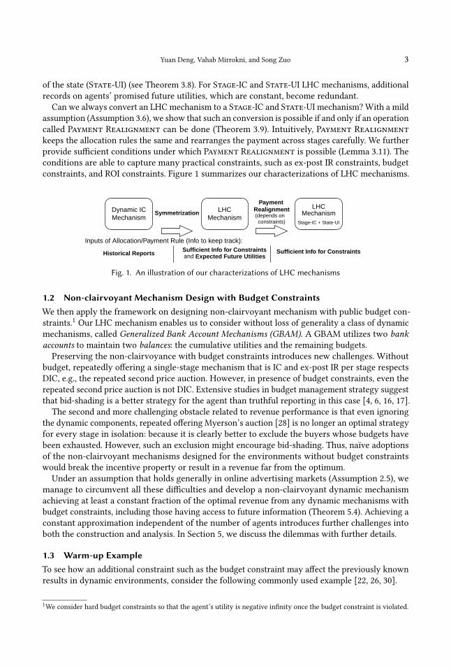
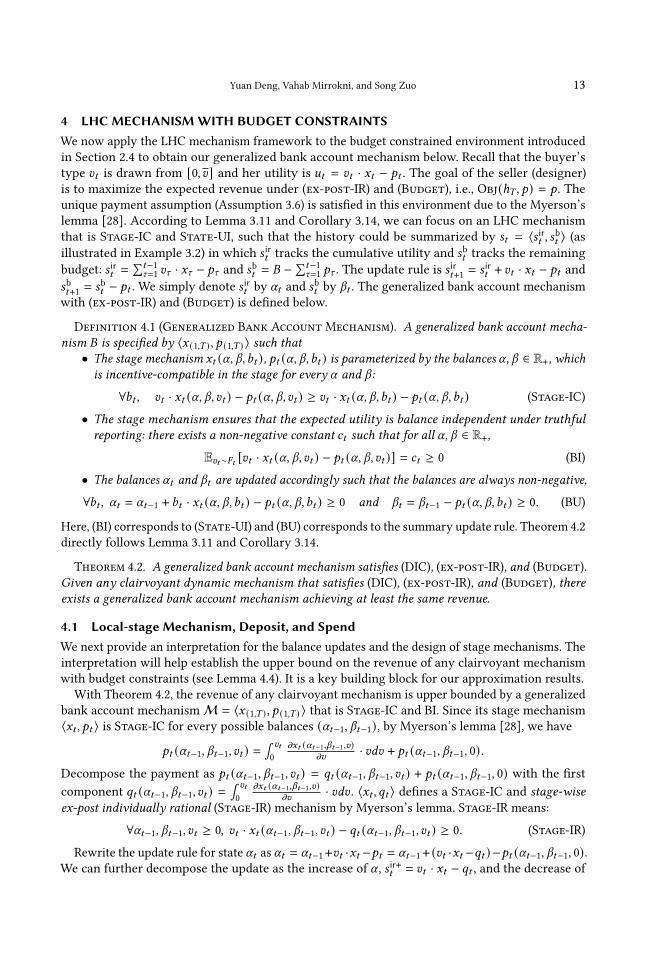
Can we always convert an LHC mechanism to a Stage-IC and State-UImechanism?With a mildassumption (Assumption 3.6), we show that such an conversion is possible if and only if an operationcalled Payment Realignment can be done (Theorem 3.9). Intuitively, Payment Realignmentkeeps the allocation rules the same and rearranges the payment across stages carefully. We furtherprovide sufficient conditions under which Payment Realignment is possible (Lemma 3.11). Theconditions are able to capture many practical constraints, such as ex-post IR constraints, budgetconstraints, and ROI constraints. Figure 1 summarizes our characterizations of LHC mechanisms.

LHC

Stage-IC + State-UI

Symmetrization

Inputs of Allocation/Payment Rule (Info to keep track):

Historical Reports Sufficient Info for Constraints Sufficient Info for Constraintsand Expected Future Utilities

PaymentRealignment

MechanismLHCMechanism (depends on

constraints)

Dynamic ICMechanism

Fig. 1. An illustration of our characterizations of LHC mechanisms

1.2 Non-clairvoyant Mechanism Design with Budget ConstraintsWe then apply the framework on designing non-clairvoyant mechanism with public budget con-straints.1 Our LHC mechanism enables us to consider without loss of generality a class of dynamicmechanisms, called Generalized Bank Account Mechanisms (GBAM). A GBAM utilizes two bank

accounts to maintain two balances: the cumulative utilities and the remaining budgets.Preserving the non-clairvoyance with budget constraints introduces new challenges. Without

budget, repeatedly offering a single-stage mechanism that is IC and ex-post IR per stage respectsDIC, e.g., the repeated second price auction. However, in presence of budget constraints, even therepeated second price auction is not DIC. Extensive studies in budget management strategy suggestthat bid-shading is a better strategy for the agent than truthful reporting in this case [4, 6, 16, 17].

The second and more challenging obstacle related to revenue performance is that even ignoringthe dynamic components, repeated offering Myerson’s auction [28] is no longer an optimal strategyfor every stage in isolation: because it is clearly better to exclude the buyers whose budgets havebeen exhausted. However, such an exclusion might encourage bid-shading. Thus, naïve adoptionsof the non-clairvoyant mechanisms designed for the environments without budget constraintswould break the incentive property or result in a revenue far from the optimum.

Under an assumption that holds generally in online advertising markets (Assumption 2.5), wemanage to circumvent all these difficulties and develop a non-clairvoyant dynamic mechanismachieving at least a constant fraction of the optimal revenue from any dynamic mechanisms withbudget constraints, including those having access to future information (Theorem 5.4). Achieving aconstant approximation independent of the number of agents introduces further challenges intoboth the construction and analysis. In Section 5, we discuss the dilemmas with further details.

1.3 Warm-up ExampleTo see how an additional constraint such as the budget constraint may affect the previously knownresults in dynamic environments, consider the following commonly used example [22, 26, 30].

1We consider hard budget constraints so that the agent’s utility is negative infinity once the budget constraint is violated.


Basic Setting. A seller sells two items to one buyer in two periods. The buyer has additivevaluation and quasi-linear utility. The buyer’s private values 𝑣1, 𝑣2 ∼ 𝐹 are drawn independently atthe beginning of each stage, respectively. 𝐹 is an equal-revenue distribution with largest value 𝑣 :

Pr[𝑣1 ≤ 𝑣] = Pr[𝑣2 ≤ 𝑣] = 𝐹 (𝑣) =

0, 𝑣 ∈ [0, 1]1 − 1/𝑣, 𝑣 ∈ (1, 𝑣)1, 𝑣 ≥ 𝑣

.

The revenue optimal static mechanism, with two items sold independently, yields revenue 2 bysetting a price 1 for each. However, the following revenue optimal dynamic mechanism yieldsexpected revenue 2+ln ln 𝑣 , while incentivizing the buyer to always participate and report truthfully:(1) In the first stage, the buyer reports her private type as 𝑣1. If 𝑣1 ≥ 1, the item is sold at price

𝑟1 = min{𝑣1, 1 + ln 𝑣}; otherwise, the item is not sold and we set 𝑟1 = 1.(2) In the second stage, the buyer reports her private type as 𝑣2 and the seller sells the item via a

posted-price auction with price 𝑟2 = 𝑣/𝑒𝑟1−1.The dynamicmechanism above is ex-post individually rational, because in neither stage the paymentis larger than the reported value. Truthful-reporting is the best strategy, because: i) for given 𝑟1, theauction in the second stage is a posted-price auction; ii) given best-response (truthful reporting) inthe second stage, the expected utility at the second stage for any 1 ≤ 𝑟2 ≤ 𝑣 is

E𝑣2∼𝐹

[(𝑣2 − 𝑟2)+] =∫ 𝑣

𝑟2

(𝑣2 − 𝑟2)𝑑𝐹 (𝑣2) + Pr[𝑣2 = 𝑣] · (𝑣 − 𝑟2) = ln 𝑣 − ln 𝑟2 .

Therefore, the cumulative expected utility of reporting 𝑣1 ≥ 1 is

1{𝑣1 ≥ 1} · (𝑣1 − 𝑟1) + E𝑣2∼𝐹

[(𝑣2 − 𝑟2)+] = 𝑣1 − 𝑟1 + ln 𝑣 − ln(𝑣/𝑒𝑟1−1) = 𝑣1 − 1,

where (𝑥)+ = max(𝑥, 0), while the expected utility of reporting 𝑣1 < 1 is zero. The expected revenueis E[1{𝑣1 ≥ 1} · 𝑟1 + 1(𝑣2 ≥ 𝑟2) · 𝑟2] = 2 + ln ln 𝑣 ≫ 2.

Bank Account Mechanism. The above can be reformulated as a bank account mechanism [26]:(1) In the first stage, the buyer reports her value as 𝑣1 and the item is sold at a posted-price 1.(2) Let the bank account balance be 𝛼 = min{ln 𝑣, (𝑣1 − 1)+};(3) In the second stage, before 𝑣2 is drawn, the buyer pays 𝛼 ; then the buyer realizes 𝑣2 and

reports 𝑣2; finally, the item is sold at a posted-price 𝑟2 = 𝑣/𝑒𝛼 .The only difference between the two mechanisms is that we postpone a payment 𝛼 = 𝑟1 − 1 fromthe first stage to the beginning of the second stage in the bank account mechanism. In fact, theexpected utility from the second stage is always zero: E[(𝑣2 − 𝑟2)+] − 𝛼 = ln 𝑣 − ln(𝑣/𝑒𝛼 ) − 𝛼 ≡ 0.Such a property is later formalized as BI or State-UI. Moreover, the buyer is incentivized to reporttruthfully in the posted-price auction of the first stage even if the second stage may not exist.

With Budget Setting. Consider the case in which the buyer is subject to a budget constraint𝐵 ∈ (2, 𝑣). Then the buyer cannot afford the second item when 𝑣1 < ln 𝑣 − ln𝐵 + 1 so that 𝑟2 > 𝐵.In this case, the previous mechanism is no longer truthful for a buyer with 1 ≤ 𝑣1 < ln 𝑣 − ln𝐵 + 1.Note that truthful reporting yields expected utility −∞, since 𝐵 < 𝑟2 ≤ 𝑣 and it is possible that𝑣2 ≥ 𝑟2. On the other hand, misreporting 𝑣1 = 1 yields utility 𝑣1−𝑣1 +0 = 𝑣1−1 ≥ 0. Fortunately, wecan fix the mechanism by replacing 𝑟1 and 𝑟2 with 𝑟 ′1 = min{𝑣1, 1+ ln(𝐵− 1)} and 𝑟 ′2 = (𝐵− 1)/𝑒𝑟 ′1−1,respectively. One can verify that 𝑟 ′1 + 𝑟 ′2 never exceeds 𝐵 and hence the budget constraint andtruthfulness are respected. In this case, the expected revenue drops to 2 + ln ln(𝐵 − 1).

However, this may not be the optimal dynamic mechanism anymore. To see this, let 𝐵 < 2 + ln 𝑣and consider the variation with 𝑟1 replaced by 𝑟 ′′1 = min{𝑣1, 𝐵} and the auction in the secondstage changed to allocate the item for free with probability (𝑟 ′′1 − 1)/(1 + ln 𝑣) (well-defined when


𝐵 < 2+ ln 𝑣). We omit the analysis here but conclude that this new mechanism is dynamic incentive-compatible and yields expected revenue 1 + ln𝐵 ≫ 2 + ln ln(𝐵 − 1), when 𝐵 is sufficiently large.

Finally, we highlight that the problem of designing (approximately) revenue-optimal mechanismcan be very different under the settings with and without budgets. The budget constraint bringsup many new challenges. Our example demonstrates that a direct generalization of the revenue-optimal mechanism under the without-budget setting could yield a revenue𝑂 (ln ln𝐵), which couldbe much less than the revenue 𝑂 (ln𝐵) of the mechanism properly designed for budget constraints.

1.4 Related WorkDynamic Mechanism Design. There is a large body of literature on dynamic mechanism design.

We briefly discuss those closely related to ours, while refer readers to Bergemann and Välimäki [9]for a comprehensive survey. Bergemann and Välimäki [8] propose a welfare-maximizing dynamicpivot mechanism that is a generalization of the VCG mechanism to the dynamic environmentwhere the buyers receive their private information over time. A team mechanism achieving efficientand budget-balanced outcomes is proposed by Athey and Segal [3]. Another related line of researchis on revenue-maximization dynamic mechanism design: Pavan et al. [31] extend the Myersonianapproach [28] and characterize dynamic incentive-compatibility, and Papadimitriou et al. [30]shows an arbitrarily large revenue gap between static and dynamic mechanisms.

Dynamic Mechanism Design Framework. The promised utility framework was proposed byThomas and Worrall [34]. Ashlagi et al. [2] design a revenue-utility tradeoff framework. Our workgeneralizes the framework by Mirrokni et al. [24, 26]. They provide the bank account mechanismframework to design the dynamic mechanism with simple structures. Based on their framework,Mirrokni et al. [26] design a non-clairvoyant mechanism which, surprisingly, achieves a constantfraction of the revenue of the optimal clairvoyant mechanism. Mirrokni et al. [25] proposes practicalbank account mechanisms and huge revenue lifts have been found from experiments.

1.5 OrganizationIn Section 2, we introduce a general environment for dynamicmechanism design, andwe present ourLHC framework in Section 3. We define the LHC mechanism with budgets, coined generalized bankaccount mechanisms, in Section 4, and derive an upper-bound on the revenue of any clairvoyantmechanism with budgets. We present our non-clairvoyant mechanism with budgets in Section 5.

2 A GENERAL DYNAMIC ENVIRONMENT2.1 Dynamic EnvironmentsWe consider the problem of a single designer (he) running a dynamic mechanism among the sameset of self-interested agents, i.e., {1, . . . , 𝑛}, for𝑇 > 0 stages. For the sake of clarity, we focus on thesingle agent (she) case and all our results for LHC mechanisms (Section 3) can be generalized tomulti-agent settings without changes in the proofs. In each stage 𝑡 , there is a newly arrived itemand the designer must determine the allocation of the item once it arrives.The agent realizes her private type \𝑡 ∈ Θ𝑡 after she observes the item, and under allocation

𝑥𝑡 ∈ X𝑡 , she receives value 𝑣𝑡 (\𝑡 , 𝑥𝑡 ), where 𝑣𝑡 : X𝑡 × Θ𝑡 → R. The private type at each stage 𝑡 isindependently drawn according to the prior distribution 𝐹𝑡 ∈ F𝑡 . However, the distributions arenot necessarily identical across stages. In the main content of this paper, we focus on the settingwith independent valuations where 𝐹𝑡 is invariant of the history. In Appendix A, we argue that ourframework can be extended to a more general setting with public valuation correlations. There, weallow 𝐹𝑡 to vary with any publicly observable information from the past of the mechanism, such as


the historical allocations, and therefore, many important valuation models can also be captured inour framework. We refer readers to Appendix B for the details of our modeling choices.

Definition 2.1 (History). A history ℎ𝑡 ∈ H𝑡 consists of the historical reports of the agent’s

private types, i.e., \̂ (1,𝑡 ) , and the sequence of mechanism outcomes until the end of stage 𝑡 , including

the historical allocation ⟨𝑥1, . . . , 𝑥𝑡 ⟩ and even the realizations of randomized outcomes.

Along with the allocation, there could be a monetary transfer from the agent to the designer, orsimply referred as payment 𝑝𝑡 ∈ R. Henceforth, the agent obtains stage utility 𝑢𝑡 = 𝑣𝑡 (\𝑡 , 𝑥𝑡 ) − 𝑝𝑡 ,and therefore her cumulative utility from the entire dynamic mechanism is 𝑢 =

∑𝑡 ∈[𝑇 ] 𝑢𝑡 .

2.2 Clairvoyant Dynamic MechanismsWe first introduce the notational basis with the mechanisms in which the prior knowledge isavailable to the designer from the beginning. Such mechanisms are termed clairvoyant dynamic

mechanisms. Later in Section 2.3, we define the non-clairvoyant dynamic mechanisms, in which theprior knowledge of each stage is revealed to the designer at the beginning of that stage.

In a clairvoyant dynamic mechanism, the designer knows the number of stages𝑇 and the sequenceof priors 𝐹1, . . . , 𝐹𝑇 in advance. Hence the mechanism enjoys the ability of forecasting the future.

We focus on direct mechanisms throughout this paper (both in clairvoyant and non-clairvoyantsettings), where the agent repeatedly reports her private types in each stage as \̂𝑡 ∈ Θ𝑡 . In each stageof a clairvoyant mechanism, upon receiving the report \̂𝑡 , the designer decides and implementsthe stage outcome based on the history ℎ𝑡−1 and the priors, 𝐹 (1,𝑇 ) = (𝐹1, · · · , 𝐹𝑇 ). Throughout thepaper, we will use the notation 𝑎 (𝑡 ′,𝑡 ′′) to represent the sequence of 𝑎 between stage 𝑡 ′ and 𝑡 ′′.

Formally, we define a clairvoyant mechanism via the allocation and payment rules based on ℎ𝑡−1.

Definition 2.2 (Clairvoyant Dynamic Mechanism). A clairvoyant dynamic mechanism is

defined by a pair of allocation and payment rules ⟨𝑥 (1,𝑇 ) , 𝑝 (1,𝑇 )⟩:• Allocation rule 𝑥𝑡 (ℎ𝑡−1, \̂𝑡 , 𝐹 (1,𝑇 ) ), 𝑥𝑡 : H𝑡−1 × Θ𝑡 × (F1 × · · · × F𝑇 ) → X𝑡 ;• Payment rule 𝑝𝑡 (ℎ𝑡−1, \̂𝑡 , 𝐹 (1,𝑇 ) ), 𝑝𝑡 : H𝑡−1 × Θ𝑡 × (F1 × · · · × F𝑇 ) → R.

Therefore, the allocation and payment rules at stage 𝑡 of a clairvoyant mechanism can depend onthe past history, the agent’s reported type at stage 𝑡 , and the prior knowledge of all stages:

MC = ⟨𝑥𝑡 (ℎ𝑡−1, \̂𝑡 , 𝐹 (1,𝑇 ) ), 𝑝𝑡 (ℎ𝑡−1, \̂𝑡 , 𝐹 (1,𝑇 ) )⟩𝑇𝑡=1. (Clairvoyant Mechanism)

To summarize, in each stage of a clairvoyant dynamic mechanism, the following steps happen:(1) the agent observes the item and realizes her private type \𝑡 ∼ 𝐹𝑡 ;(2) the agent reports type \̂𝑡 to the designer;(3) the designer implements the allocation 𝑥𝑡 (ℎ𝑡−1, \̂𝑡 , 𝐹 (1,𝑇 ) ) and the payment 𝑝𝑡 (ℎ𝑡−1, \̂𝑡 , 𝐹 (1,𝑇 ) );(4) the agent accrues stage utility 𝑢𝑡 = 𝑣𝑡

(\𝑡 , 𝑥𝑡 (ℎ𝑡−1, \̂𝑡 , 𝐹 (1,𝑇 ) )

)− 𝑝𝑡 (ℎ𝑡−1, \̂𝑡 , 𝐹 (1,𝑇 ) ).

In the rest of the paper, we hide the prior knowledge 𝐹 (1,𝑇 ) from the inputs to clairvoyant mecha-nisms when there is no ambiguity, e.g., we write 𝑢𝑡 (ℎ𝑡−1, \̂𝑡 ;\𝑡 ) = 𝑣𝑡

(\𝑡 , 𝑥𝑡 (ℎ𝑡−1, \̂𝑡 )

)− 𝑝𝑡 (ℎ𝑡−1, \̂𝑡 ).

In addition to the definitions above, a valid clairvoyant mechanism must meet certain incentiveguarantees (see Section 2.2.1) and outcome restrictions (see Section 2.2.2).

2.2.1 Dynamic Incentive Compatibility. The agent’s best response in a dynamic mechanism dependson her strategy in the future stages. The classic notion of dynamic incentive-compatibility requiresthat for all stages, reporting truthfully is the optimal strategy, assuming that she reports truthfullyin the future [26].2 Notice that reporting truthfully is also the buyer’s optimal strategy in the future,2Interested readers can refer to [26] for discussions on the choice of DIC notions.


assuming the mechanism is dynamic incentive-compatible in the future. For a history ℎ𝑡 , let thecontinuation utility be𝑈 𝑡 (ℎ𝑡 ) = E

[∑𝑇𝜏=𝑡+1 𝑢𝜏 (ℎ𝜏−1, \𝜏 ;\𝜏 )

], the expected utility from the remaining

stages via truthful reporting, where ℎ𝜏 is the history at stage 𝜏 > 𝑡 resulted from truthful reportingfrom stage 𝑡 + 1 to 𝜏 after ℎ𝑡 . The expectation here is taken over the random events in the remainingstage and the private type draws \𝜏 ∼ 𝐹𝜏 .

To highlight the effects from the agent’s report \̂𝑡 at stage 𝑡 , let ℎ (𝑡 )𝑡 be the history obtained fromℎ𝑡−1 where the agent reports \̂𝑡 at stage 𝑡 , and denote by ℎ (𝑡 )𝜏 a history at stage 𝜏 > 𝑡 resulted fromreporting truthfully from stage 𝑡 + 1 to 𝜏 after ℎ (𝑡 )𝑡 ; and thus, the continuation utility is given by:

𝑈 𝑡(ℎ(𝑡 )𝑡

)= E

[∑𝑇𝜏=𝑡+1 𝑢𝜏 (ℎ

(𝑡 )𝜏−1, \𝜏 ;\𝜏 )

].

Dynamic incentive compatibility can then be defined via backward induction: in the last stage 𝑇 , itis an optimal strategy for the agent to report truthfully no matter what the history ℎ𝑇−1 is:

\𝑇 ∈ argmax\̂𝑇𝑢𝑇 (ℎ𝑇−1, \̂𝑇 ;\𝑇 ),

for all private type \𝑇 and history ℎ𝑇−1. For the induction step, in stage 𝑡 , conditioned on theagent reporting truthfully for all the remaining stages, the agent should be incentivized to reporttruthfully no matter what the history ℎ𝑡−1 is:

∀𝑡 ∈ [𝑇 ], \𝑡 ∈ Θ𝑡 , ℎ𝑡−1 ∈ H𝑡−1, \𝑡 ∈ argmax\̂𝑡𝑢𝑡 (ℎ𝑡−1, \̂𝑡 ;\𝑡 ) +𝑈 𝑡

(ℎ(𝑡 )𝑡

). (DIC)

2.2.2 MechanismConstraints. As the second novelty of our general design framework, we introducethe general constraints on the mechanism outcomes. The practical constraints beyond the canonicalex-post individually rational constraints then can directly fit into our framework.In a seminal work, Mirrokni et al. [26] introduces a design framework called bank account

mechanisms to simplify the design of dynamic mechanisms with respect to the ex-post individualrationality. This paper focuses on empowering the general LHC framework to incorporate practicalconstraints, such as budget constraints, return on investment (ROI) constraints, etc.More specifically, we allow most constraints on the mechanism outcomes as long as they are

independent of the agent private types.3 The constraints may involve any public informationlike priors and the reported types. Examples include the ex-post or ex-ante individually rationalconstraint, the budget constraint (agents could even have separate budgets for items of differentcategories), ROI constraints, supply or demand constraints, etc. Nevertheless, the DIC constraintdoes not belong to this category, as it depends on the private types.

Without loss of generality, we classify the constraints into two categories: allocation constraints

and payment constraints, denoted by X and P , respectively (font-variants of 𝑥 and 𝑝).

Definition 2.3 (Allocation Constraints). The allocation constraints X = ⟨X1, . . . ,X𝑇 ⟩.Each X𝑡 maps the history ℎ𝑡−1, the agent’s reported type \̂𝑡 , and priors 𝐹 (1,𝑇 ) to a subset of X𝑡 :4

𝑥𝑡 ∈ X𝑡 (ℎ𝑡−1, \̂𝑡 , 𝐹 (1,𝑇 ) ) ⊆ X𝑡 . (Allocation)

In this paper, we will simply write it as 𝑥𝑡 ∈ X𝑡 when there is no ambiguity.

In addition to the above definition, we further assume the allocation constraints X is monotone:∀𝑥 ′𝑡 ∈ X𝑡 , \̂𝑡+1 ∈ Θ𝑡+1, X𝑡+1 (ℎ′𝑡 , \̂𝑡+1, 𝐹 (1,𝑇 ) ) ≠ ∅, where ℎ′𝑡 is the history when the allocation instage 𝑡 is set to be 𝑥 ′𝑡 . The assumption essentially requires the constraints to early rule out theallocations that can lead to no feasible outcomes later.3The feasible set of the constraints must be a properly measurable set such that all the expectation operators are well-defined.4As the history ℎ𝑡−1 includes all the historical information, the definition is almost universal. We won’t get too much intothe mathematical details, while note that both X𝑡 and P𝑡 are properly defined measurable functions.


Definition 2.4 (Payment Constraints). The payment constraints P = ⟨P1, . . . , P𝑇 ⟩. EachP𝑡 maps the history ℎ𝑡−1, the allocation of the current stage 𝑥𝑡 , past payments 𝑝 (1,𝑡−1) , the agent’s

reported type \̂𝑡 , and priors 𝐹 (1,𝑇 ) to a subset of R:

𝑝𝑡 ∈ P𝑡 (ℎ𝑡−1, 𝑥𝑡 , 𝑝 (1,𝑡−1) , \̂𝑡 , 𝐹 (1,𝑇 ) ) ⊆ R. (Payment)Similarly, we write it as 𝑝𝑡 ∈ P𝑡 and assume the payment constraints P to be monotone.

As a quick example, the ex-post IR constraints can be defined as part of the payment constraints.

2.2.3 Designer Objective. Finally, we allow an abstract objective for the designer:Obj(ℎ𝑇 , 𝑝) : H𝑇 × R→ R, (Objective)

where 𝑝 =∑𝑡 ∈[𝑇 ] 𝑝𝑡 is the total payment. We summarize the design problem as a program

maximize E[Obj(ℎ𝑇 , 𝑝)] (Design Problem)subject to (DIC) and 𝑥𝑡 ∈ X𝑡 , 𝑝𝑡 ∈ P𝑡 , ∀𝑡 ∈ [𝑇 ] .

As a quick example, the objective can be to maximize revenue by setting Obj(ℎ𝑇 , 𝑝) = 𝑝 .

2.3 Non-clairvoyant Dynamic MechanismThe non-clairvoyance notion is first introduced by Mirrokni et al. [26] to remove the unrealisticdesigner power of forecasting the distributional information and arriving order of future items. Adesigner is non-clairvoyant, if he does not know the value of 𝑇 and has no access to 𝐹𝑡 until thebeginning of stage 𝑡 . A dynamic mechanism is non-clairvoyant, if its allocation and payment rulesare independent of the prior knowledge of future stages, 𝐹 (𝑡+1,𝑇 ) , and the total number of stages, 𝑇 :

MNC = ⟨𝑥𝑡 (ℎ𝑡−1, \̂𝑡 , 𝐹 (1,𝑡 ) ), 𝑝𝑡 (ℎ𝑡−1, \̂𝑡 , 𝐹 (1,𝑡 ) )⟩∞𝑡=1 . (Non-clairvoyant Mechanism)

A mechanism is dynamic incentive compatible in the non-clairvoyant sense, if it respects (DIC)for all𝑇 ∈ N and any priors 𝐹 (𝑡+1,𝑇 ) of future stages. Taking𝑇 = 𝑡 (consider stage 𝑡 as the last stage),we get stage-wise incentive compatible, because the corresponding continuation utility𝑈 𝑡 = 0:

(DIC) =⇒ \𝑡 ∈ argmax\̂𝑡𝑢𝑡 (ℎ𝑡−1, \̂𝑡 ;\𝑡 ) +𝑈 𝑡

(ℎ(𝑡 )𝑡

)= argmax

\̂𝑡𝑢𝑡 (ℎ𝑡−1, \̂𝑡 ;\𝑡 ). (Stage-IC)

Finally, the mechanism constraints must respect the non-clairvoyance as well,

𝑥𝑡 ∈ X𝑡 (ℎ𝑡−1, \̂𝑡 , 𝐹 (1,𝑡 ) ) ⊆ X𝑡 , 𝑝𝑡 ∈ P𝑡 (ℎ𝑡−1, 𝑥𝑡 , 𝑝 (1,𝑡−1) , \̂𝑡 , 𝐹 (1,𝑡 ) ) ⊆ R.

2.4 Ad Auctions with Budget Constrained BuyersAs we mentioned before, we are particularly interested in the practical setting of ad auctionswith budget constrained buyers. In particular, we consider an environment with allocation spaceX𝑡 = [0, 1], type space Θ𝑡 = [0, 𝑣], and quasi-linear utility 𝑢𝑡 = \𝑡𝑥𝑡 − 𝑝𝑡 . Moreover, the following(ex-post-IR) constraint and (Budget) constraint must be satisfied by the industrial standard:

Pex-post-IR ={𝑝 =

∑𝑡 ∈[𝑇 ] 𝑝𝑡 ≤

∑𝑡 ∈[𝑇 ] 𝑣𝑡 (\̂𝑡 , 𝑥𝑡 )

}(ex-post-IR)

PBudget ={𝑝 =

∑𝑡 ∈[𝑇 ] 𝑝𝑡 ≤ 𝐵

}(Budget)

Therefore, the mechanism constraint is P = Pex-post-IR ∩PBudget, which must be satisfied for all𝑇 ∈ N in the non-clairvoyant mechanisms.

The objective of the designer is to design a revenue-optimal mechanism that satisfies (DIC),(ex-post-IR), and (Budget) in clairvoyant and non-clairvoyant environments. The following mildassumption applies for our approximation analysis of our non-clairvoyant mechanism in the budgetconstrained environment, which is motivated by the online advertising market where the buyer’sbudget is typically much larger than her valuation of every possible impression.


Assumption 2.5. There exists a sufficiently small 𝜖 such that the buyer’s budget satisfies 𝐵 ≥ 𝑣/𝜖 .Remark 2.6. Our characterizations in Section 3 and Section 4 do not rely on Assumption 2.5, but

our non-clairvoyant mechanism in Section 5 does. We note that Assumption 2.5 rules out the budgeted

scenario we discussed in Section 1.3. However, designing a non-clairvoyant mechanism under budget

constraints with non-trivial revenue guarantee under Assumption 2.5 is already technically involved.We

leave it as an interesting open question to design non-clairvoyant mechanisms without Assumption 2.5.

3 LOSSLESS HISTORY COMPRESSION (LHC) MECHANISMIn this section, we formally define our general design framework that we call Lossless HistoryCompression (LHC) mechanisms, which serves as the bridge that connects clairvoyant dynamicmechanism designs and non-clairvoyant dynamic mechanism designs. We defer the proofs in thissection to Appendix C. LHC mechanisms generalize the idea of the bank account mechanisms, atechnique introduced by Mirrokni et al. [24, 26] for the classic ex-post individually rational con-straints. Moreover, the design of optimal clairvoyant dynamic mechanisms can be restricted to LHCmechanisms, without losing any generality in terms of the designer Objective (see Theorem 3.5).

At a high level, in an LHC mechanism (see Definition 3.3), a succinct summary of the historicalinformation, which we call it state, is used to keep track on the least information that is essentialfor implementing the dynamic mechanism. The information is compressed as much as possible tosimplify the structure of the dynamic mechanism, while not violating any mechanism constraintsnor losing any prior knowledge information (for the general setting with public correlations). Thefollowing notion of lossless history compression then defines the least information to be kept.Definition 3.1 (Lossless History Compression (LHC)). A lossless history compression (or

simply compression) 𝑠 = ⟨𝑠1, . . . , 𝑠𝑇 ⟩ is a sequence of functions — each maps the history and previous

payments to a succinct summary 𝑠𝑡 (ℎ𝑡 , 𝑝 (1,𝑡 ) ), i.e., 𝑠𝑡 : H𝑡 × R𝑡 → S𝑡 — such that there exist

accompanying mechanism constraints ⟨X̃𝑡 , P̃𝑡 ⟩ defined on 𝑠𝑡 ,X̃𝑡 (𝑠𝑡−1, \̂𝑡 , 𝐹 (1,𝑇 ) ) = X𝑡 (ℎ𝑡−1, \̂𝑡 , 𝐹 (1,𝑇 ) ),

P̃𝑡 (𝑠𝑡−1, 𝑥𝑡 , \̂𝑡 , 𝐹 (1,𝑇 ) ) = P𝑡 (ℎ𝑡−1, 𝑥𝑡 , 𝑝 (1,𝑡−1) , \̂𝑡 , 𝐹 (1,𝑇 ) ),

and a summary update rule Λ = ⟨Λ1, . . . ,Λ𝑇 ⟩: 𝑠𝑡 (ℎ𝑡 , 𝑝 (1,𝑡 ) ) = Λ𝑡 (𝑠𝑡−1 (ℎ𝑡−1, 𝑝 (1,𝑡−1) ), \̂𝑡 , 𝑥𝑡 , 𝑝𝑡 ).Intuitively, the compression contains the sufficient information to perfectly recover the mecha-

nism constraints as ⟨X̃𝑡 , P̃𝑡 ⟩, and it can be tracked by the update rule 𝑠𝑡 = Λ𝑡 (𝑠𝑡−1, \̂𝑡 , 𝑥𝑡 , 𝑝𝑡 ). Ata glance, the abstract definition above seems complicated, yet it turns out to be quite simple formost of the common settings, where each of the constraints may end up with one real number inthe summary. As a quick example, let’s consider the (ex-post-IR) and (Budget) constraints, whichwill be further investigated in Section 4.

Example 3.2 (ex-post-IR and Budget). Let S𝑡 = R2 and each summary 𝑠𝑡 be two real numbers

⟨𝑠 ir𝑡 , 𝑠b𝑡 ⟩ for the (ex-post-IR) and (Budget) constraints, respectively. The compression is defined as:

𝑠 ir𝑡 =∑𝑡𝜏=1 𝑣𝜏 (\̂𝜏 , 𝑥𝜏 ) − 𝑝𝜏 and 𝑠b𝑡 = 𝐵 − ∑𝑡

𝜏=1 𝑝𝜏 . These constraints could be easily recovered as

P̃ex-post-IR

𝑇 = {𝑝𝑇 ≤ 𝑠 ir𝑇−1 + 𝑣𝑇 (\̂𝑇 , 𝑥𝑇 )} and P̃Budget

𝑇 = {𝑝𝑇 ≤ 𝐵 − 𝑠b𝑇−1}.

Finally, the summary is updated according to 𝑠 ir𝑡 = 𝑠 ir𝑡−1 + 𝑣𝑡 (\̂𝑡 , 𝑥𝑡 ) − 𝑝𝑡 and 𝑠b𝑡 = 𝑠b𝑡−1 − 𝑝𝑡 .We are now ready to formally define an LHC mechanism.

Definition 3.3 (LHC Mechanism). An LHC mechanism M̃ = ⟨𝑥, 𝑝⟩ is defined based on a lossless

history compression 𝑠 with 𝜎𝑡 = ⟨𝑠𝑡 , `𝑡 ⟩ as its state, where `𝑡 = 𝑈𝑡 (𝜎𝑡 ) is the promised continuationutility.5 In each stage 𝑡 ,


(1) the agent realizes her private type \𝑡 , reports \̂𝑡 , and accrues stage utility 𝑢𝑡 (𝜎𝑡−1, \̂𝑡 ;\𝑡 ) =

𝑣𝑡

(\𝑡 , 𝑥𝑡 (𝜎𝑡−1, \̂𝑡 )

)−𝑝𝑡 (𝜎𝑡−1, \̂𝑡 ) from the stage allocation 𝑥𝑡 (𝜎𝑡−1, \̂𝑡 ) and payment 𝑝𝑡 (𝜎𝑡−1, \̂𝑡 );

(2) the next state 𝜎𝑡 is determined according to the following state update rule

𝜎𝑡 = ⟨𝑠𝑡 , `𝑡 ⟩ = ⟨Λ𝑡 (𝑠𝑡−1, \̂𝑡 , 𝑥𝑡 , 𝑝𝑡 ), `𝑡 (𝜎𝑡−1, \̂𝑡 )⟩, (State-Update)

where E\𝑡∼𝐹𝑡 [𝑢𝑡 (𝜎𝑡−1, \𝑡 ;\𝑡 ) + `𝑡 (𝜎𝑡−1, \𝑡 )] = `𝑡−1;(3) the stage outcome ⟨𝑥𝑡 , 𝑝𝑡 ⟩ satisfies the following incentive constraint

\𝑡 ∈ argmax\̂𝑡𝑢𝑡 (𝜎𝑡−1, \̂𝑡 ;\𝑡 ) + `𝑡 (𝜎𝑡−1, \̂𝑡 ), (LHC-IC)

and the allocation and payment constraints 𝑥𝑡 ∈ X̃𝑡 , 𝑝𝑡 ∈ P̃𝑡 .

Our key result is that without loss of generality, one can find an optimal solution to the DesignProblem within LHC mechanisms. On one hand, by putting the definitions together (Definition 3.1,Definition 3.3, and (DIC), (Allocation), (Payment) constraints), we can directly conclude:

Lemma 3.4. Any LHC mechanism satisfies (DIC), (Allocation), and (Payment) constraints.

On the other hand, as we will prove in Section 3.3 by construction, one can reduce any dynamicmechanism to a LHC mechanism without losing the optimality.

Theorem 3.5. Given any dynamic mechanism satisfying (DIC), (Allocation), and (Payment)constraints, for any given lossless history compression 𝑠 , there exists an LHC mechanism defined based

on 𝑠 that yields at least the same designer Objective. In particular, the optimal solution to the Design

Problem can be achieved by an optimal LHC mechanism.

3.1 Non-clairvoyance, Stage-Incentive Compatibility, and State-Utility IndependenceBefore we provide a proof sketch for Theorem 3.5, we first establish the connection between LHCmechanisms and non-clairvoyant dynamicmechanisms.We first introduce two important propertiesclosely related to the non-clairvoyant notions: stage IC and state-utility independence. Firstly, undera mild assumption (Assumption 3.6) that holds for most commonly studied environments, weprove that these two properties together is an if-and-only-if characterization of non-clairvoyantmechanisms satisfying non-clairvoyant (DIC). Moreover, any dynamic mechanism can be convertedto stage IC and state-utility independent mechanism without loss of optimality when the (Payment)constraints satisfy a further property (see Theorem 3.8) such that (Payment Realignment) ispossible. Secondly, we show in Corollary 3.14, when these two properties are in place, we canfurther restrict our attention to a subset of LHC mechanisms with even simpler structures, wherethe state is simplified as 𝜎𝑡 = ⟨𝑠𝑡 ⟩ rather than 𝜎𝑡 = ⟨𝑠𝑡 , `𝑡 ⟩ (which is a major simplification when theupdate rule for `𝑡 is not constructive), and the (LHC-IC) constraint is also simplified as (Stage-IC).The mild assumption required is that the payment rule implementing the stage allocation 𝑥𝑡

is unique up to a constant, which is commonly satisfied in many standard environments. Forexample, the environments with continuous type spaces and additive valuations, in which the mildassumption is implied by the Myerson’s lemma [28] (in single-dimensional environments) or theenvelope theorem [32] (in multi-dimensional environments).6

5We use 𝑈𝑡 (𝜎𝑡 ) to denote the continuation utility of the LHC mechanism M̃ under state 𝜎𝑡 , which is an analog to thedefinition of𝑈 𝑡 (ℎ𝑡 ) with respect to the uncompressed history ℎ𝑡 .6The irregular cases where the assumption is violated are usually of less interests. One example is as follows. Consider asingle item auction with value space Θ𝑡 = {0, 1}. For the allocation 𝑥𝑡 (0) = 0, 𝑥𝑡 (1) = 1, any payment function such that𝑝𝑡 (0) = 0, 𝑝 (1) ∈ (0, 1] implements 𝑥𝑡 , while not satisfying the assumption.


Assumption 3.6 (Uniqe Payment). In any stage 𝑡 , every stage allocation rule 𝑥𝑡 pins down a

unique payment rule 𝑝𝑡 up to a constant 𝑐 : For any fixed history ℎ𝑡−1 and payment rule 𝑝 ′𝑡 such that

truthful reporting is an optimal strategy, i.e., \𝑡 ∈ argmax\̂𝑡𝑣𝑡

(\𝑡 , 𝑥𝑡 (ℎ𝑡−1, \̂𝑡 )) −𝑝 ′𝑡 (ℎ𝑡−1, \̂𝑡

), we have

∀\̂𝑡 ∈ Θ𝑡 , 𝑝′𝑡 (ℎ𝑡−1, \̂𝑡 ) ≡ 𝑝𝑡 (ℎ𝑡−1, \̂𝑡 ) + 𝑐, for some constant 𝑐.

As previously mentioned in Section 2.3, the non-clairvoyant (DIC) constraint directly implies(Stage-IC). In fact, it also implies the following property under Assumption 3.6:

Definition 3.7 (State-Utility Independence). An LHC mechanism is state-utility independent,if for each stage 𝑡 , there exists a constant 𝑐𝑡 such that

E\𝑡∼F̃𝑡 [𝑢𝑡 (𝜎𝑡−1, \𝑡 ;\𝑡 )] = 𝑐𝑡 independent of the state 𝜎𝑡−1 . (State-UI)

The state-utility independence property states that the agent’s expected utility at stage 𝑡 isindependent of the state 𝜎𝑡−1. Since the state 𝜎𝑡−1 is the only channel that carries the agent’shistorical reports, state-utility independence directly implies that her historical reports have noeffect on her future expected utility. Hence, a non-clairvoyant mechanism that is State-UI andStage-IC, is DIC in the non-clairvoyant sense. When Assumption 3.6 stands, we have the followingsufficient and necessary characterizations of non-clairvoyant dynamic mechanisms satisfyingnon-clairvoyant (DIC) and that dynamic mechanisms can be converted to a Stage-IC and State-UImechanism without loss of optimality.

Theorem 3.8 (Non-clairvoyance Characterization). Under Assumption 3.6, a non-clairvoyant

dynamicmechanism satisfies non-clairvoyant (DIC) if and only if it satisfies (Stage-IC) and (State-UI).

3.2 Payment RealignmentCan we convert a dynamic mechanism satisfying (DIC), (Allocation), and (Payment), to a mech-anism that is Stage-IC and State-UI? The following theorem provides a necessary and sufficientcondition, coined Payment Realignment, on when such a conversion is possible.

Theorem 3.9. AdynamicmechanismM = ⟨𝑥, 𝑝⟩ that satisfies (DIC), (Allocation), and (Payment)can be converted to a Stage-IC and State-UImechanismM ′ = ⟨𝑥, 𝑝 ′⟩ with equivalent stage allocationrules and final cumulative payment (hence the designer Objective is unaffected), if and only if there

exist constants 𝑐1, . . . , 𝑐𝑇 ∈ R such that 𝑐1 + · · · + 𝑐𝑇 = 𝑈 0 (∅) and ∀𝑡 ∈ [𝑇 ], ℎ𝑡−1 ∈ H𝑡−1, \𝑡 ∈ Θ𝑡 ,

𝑝 ′𝑡 (ℎ𝑡−1, \𝑡 ) = 𝑝𝑡 (ℎ𝑡−1, \𝑡 ) −𝑈 𝑡 (ℎ𝑡 ) +𝑈 𝑡−1 (ℎ𝑡−1) − 𝑐𝑡 ∈ P𝑡 , (Payment Realignment)

where ℎ𝑡 is the history from reporting \𝑡 after ℎ𝑡−1. Moreover, in the converted mechanism using

𝑐1, . . . , 𝑐𝑇 and Payment Realignment, the expected utility at stage 𝑡 is 𝑐𝑡 , independent of the state.

Payment Realignment keeps the allocation rule the same but rearranges the payment acrossstages. Readers may take another look at Section 1.3 for a concrete example of payment realignment.

In a non-clairvoyant environment, the agent is willing to participate in stage 𝑡 before she learns \𝑡only if her expected utility at stage 𝑡 is non-negative, which equals to 𝑐𝑡 in (Payment Realignment)by Theorem 3.9. Lemma 3.11 provides a sufficient condition under which the mechanism constraintsenables Payment Realignment with 𝑐1, · · · , 𝑐𝑇 ∈ R+ in the dynamic auction environment withΘ𝑡 = R+ for all 𝑡 . Before Lemma 3.11, we introduce the concept ofmonotone history functions, whichis a class of functions with non-decreasing function value as the dynamic mechanism proceeds.

Definition 3.10 (Monotone History Function). A function Z with Z (∅) ≤ 0 is monotone in

terms of history if for any ℎ𝑡 ∈ H𝑡 and any ℎ𝑡+1 ∈ H𝑡+1 resulted from ℎ𝑡 , Z (ℎ𝑡 ) ≤ Z (ℎ𝑡+1).


Lemma 3.11. When Θ𝑡 = R+ for all 𝑡 , Payment Realignment is possible with 𝑐1, · · · , 𝑐𝑇 ∈ R+for Payment constraints P = ⟨P1, . . . , P𝑇 ⟩ if there exist 𝛼1, · · · , 𝛼𝐾 ∈ R+ and monotone history

functions Z1, · · · , Z𝐾 such that P𝑡 ={𝑝𝑡 ∈ R : ∀𝑘 ∈ [𝐾],∑𝑡

𝜏=1 \𝜏𝑥𝜏 − (1 + 𝛼𝑘 ) · 𝑝𝜏 ≥ Z𝑘 (ℎ𝑡 )}, where

𝑥𝜏 and 𝑝𝜏 are the allocation probability and the payment at stage 𝜏 corresponding to history ℎ𝑡 .

Note that the condition of Payment constraints in Lemma 3.11 is able to capture many practicalconstraints, such as Budget, ROI constraints, and hence (ex-post-IR). For (Budget) with a budgetlimit 𝐵, set 𝛼𝑘 = 0 and Z𝑘 (ℎ𝑡 ) = −𝐵+∑𝑡

𝜏=1 \𝜏𝑥𝜏 . As for ROI constraints, which states that the agent’scumulative allocated value must be at least (1 + 𝛽) times of the agent’s cumulative payment, onecan set 𝛼𝑘 = 𝛽 and Z𝑘 (ℎ𝑡 ) = 0. (ex-post-IR) is a special case of ROI constraints with 𝛽 = 0. Onecould also think of another constraint in which the agent requires that her average utility for anyfirst 𝑡 stages must be at least 𝛾 . To represent such a constraint, set 𝛼𝑘 = 0 and Z𝑘 (ℎ𝑡 ) = 𝛾 · 𝑡 .

3.3 A Constructive Proof for Theorem 3.5We prove Theorem 3.5 by construction. The main obstacle of the proof is that for the given com-pression 𝑠 and the mechanism M = ⟨𝑥, 𝑝⟩, there might be two different histories ℎ𝑡−1 ≠ ℎ′𝑡−1, suchthat they are compressed into the same state, i.e., 𝑠𝑡−1 (ℎ𝑡−1, 𝑝 (1,𝑡−1) ) = 𝑠𝑡−1 (ℎ′𝑡−1, 𝑝 ′(1,𝑡−1) ), but thesuccessive stage allocations are different, i.e., 𝑥𝑡 (ℎ𝑡−1, \̂𝑡 ) ≠ 𝑥𝑡 (ℎ′𝑡−1, \̂𝑡 ). In this case, a direct con-struction of LHC mechanism will suffer a contradiction: 𝑥𝑡 (𝜎𝑡−1, \̂𝑡 ) = 𝑥𝑡 (𝑠𝑡−1 (ℎ𝑡−1, 𝑝 (1,𝑡−1) ), \̂𝑡 ) =𝑥𝑡 (ℎ𝑡−1, \̂𝑡 ) ≠ 𝑥𝑡 (ℎ′𝑡−1, \̂𝑡 ) = 𝑥𝑡 (𝑠𝑡−1 (ℎ′𝑡−1, 𝑝 ′(1,𝑡−1) ), \̂𝑡 ) = 𝑥𝑡 (𝜎𝑡−1, \̂𝑡 ). Therefore, a correct path is tofirst convert an arbitraryM into a symmetricmechanismMsymmetric (see Definition 3.12), and fromMsymmetric, we can easily construct an LHC mechanism M̃ such that

𝑥𝑡 (𝑠𝑡−1 (ℎ𝑡−1, 𝑝 (1,𝑡−1) ), \̂𝑡 ) = 𝑥 symmetric𝑡 (ℎ𝑡−1, \̂𝑡 ), 𝑝𝑡 (𝑠𝑡−1 (ℎ𝑡−1, 𝑝 (1,𝑡−1) ), \̂𝑡 ) = 𝑝symmetric

𝑡 (ℎ𝑡−1, \̂𝑡 ).

Definition 3.12 (Symmetric Mechanism). A mechanism M = ⟨𝑥, 𝑝⟩ is symmetric with respect

to a compression 𝑠 , if for any 𝑡 < 𝑡 ′ and two histories ℎ𝑡 , ℎ′𝑡 ∈ H𝑡 , when 𝑠𝑡 (ℎ𝑡 , 𝑝 (1,𝑡 ) ) = 𝑠𝑡 (ℎ′𝑡 , 𝑝 ′(1,𝑡 ) )and𝑈 𝑡 (ℎ𝑡 ) = 𝑈 𝑡 (ℎ′𝑡 ), we have for all \ (𝑡+1,𝑡 ′) ∈ Θ𝑡+1 × · · · × Θ𝑡 ′ ,

𝑥𝑡 ′ (ℎ𝑡 ′−1, \𝑡 ′) = 𝑥𝑡 ′ (ℎ∗𝑡 ′−1, \𝑡 ′) and 𝑝𝑡 ′ (ℎ𝑡 ′−1, \𝑡 ′) = 𝑝𝑡 ′ (ℎ∗𝑡 ′−1, \𝑡 ′), (Symmetric)

whereℎ𝑡 ′−1 andℎ∗𝑡 ′−1 are histories resulted from reporting \ (𝑡+1,𝑡 ′−1) after historyℎ𝑡 andℎ′𝑡 , respectively.

Lemma 3.13 (Symmetrization). Any dynamic mechanism M that satisfies (DIC), (Allocation),and (Payment), can be transformed into a mechanismMsymmetric

that is further Symmetric according

to the given lossless history compression 𝑠 . Moreover, Msymmetricyields at least the same designer

Objective asM, and ifM is further Stage-IC and State-UI, thenMsymmetricpreserves these properties.

The proof of Lemma 3.13 is done by applying symmetrization stage by stage, from 𝜏 = 1 to𝑇 . On each stage 𝑡 , for the histories that are mapped to the same state 𝜎𝑡 , we assign them anidentical sub-mechanism to make the entire mechanism symmetric. The assigned sub-mechanismis the sub-mechanism induced by a selected representative history that is mapped to 𝜎𝑡 with themaximum designer Objective among all the histories that are also mapped to 𝜎𝑡 . The completeproof is then a careful argument by induction. The following corollary would be useful to simplifythe states of the LHC mechanisms that are Stage-IC and State-UI.

Corollary 3.14 (Stage-IC and State-UI LHC Mechanisms). When Payment Realignment is

possible, any dynamic mechanism satisfying (DIC), (Allocation), and (Payment) can be converted

to an LHC mechanism that is Stage-IC and State-UI and yields at least the same designer Objective.

Moreover, the promised continuation utilities `𝑡 in its states 𝜎𝑡 = ⟨𝑠𝑡 , `𝑡 ⟩ at stage 𝑡 are constants, i.e., itis sufficient to keep its state simply as 𝜎𝑡 = ⟨𝑠𝑡 ⟩.


4 LHC MECHANISMWITH BUDGET CONSTRAINTSWe now apply the LHC mechanism framework to the budget constrained environment introducedin Section 2.4 to obtain our generalized bank account mechanism below. Recall that the buyer’stype 𝑣𝑡 is drawn from [0, 𝑣] and her utility is 𝑢𝑡 = 𝑣𝑡 · 𝑥𝑡 − 𝑝𝑡 . The goal of the seller (designer)is to maximize the expected revenue under (ex-post-IR) and (Budget), i.e., Obj(ℎ𝑇 , 𝑝) = 𝑝 . Theunique payment assumption (Assumption 3.6) is satisfied in this environment due to the Myerson’slemma [28]. According to Lemma 3.11 and Corollary 3.14, we can focus on an LHC mechanismthat is Stage-IC and State-UI, such that the history could be summarized by 𝑠𝑡 = ⟨𝑠 ir𝑡 , 𝑠b𝑡 ⟩ (asillustrated in Example 3.2) in which 𝑠 ir𝑡 tracks the cumulative utility and 𝑠b𝑡 tracks the remainingbudget: 𝑠 ir𝑡 =

∑𝑡−1𝜏=1 𝑣𝜏 · 𝑥𝜏 − 𝑝𝜏 and 𝑠b𝑡 = 𝐵 − ∑𝑡−1

𝜏=1 𝑝𝜏 . The update rule is 𝑠 ir𝑡+1 = 𝑠ir𝑡 + 𝑣𝑡 · 𝑥𝑡 − 𝑝𝑡 and

𝑠b𝑡+1 = 𝑠b𝑡 − 𝑝𝑡 . We simply denote 𝑠 ir𝑡 by 𝛼𝑡 and 𝑠b𝑡 by 𝛽𝑡 . The generalized bank account mechanism

with (ex-post-IR) and (Budget) is defined below.

Definition 4.1 (Generalized Bank Account Mechanism). A generalized bank account mecha-

nism 𝐵 is specified by ⟨𝑥 (1,𝑇 ) , 𝑝 (1,𝑇 )⟩ such that

• The stage mechanism 𝑥𝑡 (𝛼, 𝛽, 𝑏𝑡 ), 𝑝𝑡 (𝛼, 𝛽, 𝑏𝑡 ) is parameterized by the balances 𝛼, 𝛽 ∈ R+, whichis incentive-compatible in the stage for every 𝛼 and 𝛽 :

∀𝑏𝑡 , 𝑣𝑡 · 𝑥𝑡 (𝛼, 𝛽, 𝑣𝑡 ) − 𝑝𝑡 (𝛼, 𝛽, 𝑣𝑡 ) ≥ 𝑣𝑡 · 𝑥𝑡 (𝛼, 𝛽, 𝑏𝑡 ) − 𝑝𝑡 (𝛼, 𝛽, 𝑏𝑡 ) (Stage-IC)

• The stage mechanism ensures that the expected utility is balance independent under truthful

reporting: there exists a non-negative constant 𝑐𝑡 such that for all 𝛼, 𝛽 ∈ R+,E𝑣𝑡∼𝐹𝑡 [𝑣𝑡 · 𝑥𝑡 (𝛼, 𝛽, 𝑣𝑡 ) − 𝑝𝑡 (𝛼, 𝛽, 𝑣𝑡 )] = 𝑐𝑡 ≥ 0 (BI)

• The balances 𝛼𝑡 and 𝛽𝑡 are updated accordingly such that the balances are always non-negative,

∀𝑏𝑡 , 𝛼𝑡 = 𝛼𝑡−1 + 𝑏𝑡 · 𝑥𝑡 (𝛼, 𝛽, 𝑏𝑡 ) − 𝑝𝑡 (𝛼, 𝛽, 𝑏𝑡 ) ≥ 0 and 𝛽𝑡 = 𝛽𝑡−1 − 𝑝𝑡 (𝛼, 𝛽, 𝑏𝑡 ) ≥ 0. (BU)

Here, (BI) corresponds to (State-UI) and (BU) corresponds to the summary update rule. Theorem 4.2directly follows Lemma 3.11 and Corollary 3.14.

Theorem 4.2. A generalized bank account mechanism satisfies (DIC), (ex-post-IR), and (Budget).Given any clairvoyant dynamic mechanism that satisfies (DIC), (ex-post-IR), and (Budget), thereexists a generalized bank account mechanism achieving at least the same revenue.

4.1 Local-stage Mechanism, Deposit, and SpendWe next provide an interpretation for the balance updates and the design of stage mechanisms. Theinterpretation will help establish the upper bound on the revenue of any clairvoyant mechanismwith budget constraints (see Lemma 4.4). It is a key building block for our approximation results.

With Theorem 4.2, the revenue of any clairvoyant mechanism is upper bounded by a generalizedbank account mechanismM = ⟨𝑥 (1,𝑇 ) , 𝑝 (1,𝑇 )⟩ that is Stage-IC and BI. Since its stage mechanism⟨𝑥𝑡 , 𝑝𝑡 ⟩ is Stage-IC for every possible balances (𝛼𝑡−1, 𝛽𝑡−1), by Myerson’s lemma [28], we have

𝑝𝑡 (𝛼𝑡−1, 𝛽𝑡−1, 𝑣𝑡 ) =∫ 𝑣𝑡

0𝜕𝑥𝑡 (𝛼𝑡−1,𝛽𝑡−1,𝑣)

𝜕𝑣· 𝑣𝑑𝑣 + 𝑝𝑡 (𝛼𝑡−1, 𝛽𝑡−1, 0) .

Decompose the payment as 𝑝𝑡 (𝛼𝑡−1, 𝛽𝑡−1, 𝑣𝑡 ) = 𝑞𝑡 (𝛼𝑡−1, 𝛽𝑡−1, 𝑣𝑡 ) + 𝑝𝑡 (𝛼𝑡−1, 𝛽𝑡−1, 0) with the firstcomponent 𝑞𝑡 (𝛼𝑡−1, 𝛽𝑡−1, 𝑣𝑡 ) =

∫ 𝑣𝑡

0𝜕𝑥𝑡 (𝛼𝑡−1,𝛽𝑡−1,𝑣)

𝜕𝑣· 𝑣𝑑𝑣 . ⟨𝑥𝑡 , 𝑞𝑡 ⟩ defines a Stage-IC and stage-wise

ex-post individually rational (Stage-IR) mechanism by Myerson’s lemma. Stage-IR means:

∀𝛼𝑡−1, 𝛽𝑡−1, 𝑣𝑡 ≥ 0, 𝑣𝑡 · 𝑥𝑡 (𝛼𝑡−1, 𝛽𝑡−1, 𝑣𝑡 ) − 𝑞𝑡 (𝛼𝑡−1, 𝛽𝑡−1, 𝑣𝑡 ) ≥ 0. (Stage-IR)

Rewrite the update rule for state 𝛼𝑡 as 𝛼𝑡 = 𝛼𝑡−1+𝑣𝑡 ·𝑥𝑡 −𝑝𝑡 = 𝛼𝑡−1+ (𝑣𝑡 ·𝑥𝑡 −𝑞𝑡 )−𝑝𝑡 (𝛼𝑡−1, 𝛽𝑡−1, 0).We can further decompose the update as the increase of 𝛼 , 𝑠 ir+𝑡 = 𝑣𝑡 · 𝑥𝑡 − 𝑞𝑡 , and the decrease of


𝛼 , 𝑠 ir−𝑡 = 𝑝𝑡 (𝛼𝑡−1, 𝛽𝑡−1, 0). Thus 𝛼𝑡 = 𝛼𝑡−1 + 𝑠 ir+𝑡 − 𝑠 ir−𝑡 . In particular, 𝑠 ir+𝑡 is referred as deposit and𝑠 ir−𝑡 is referred as spend of the balance 𝛼 . We call ⟨𝑥𝑡 , 𝑞𝑡 ⟩ the local-stage mechanism. The followingalternative definition comes from the above payment decomposition.

Lemma 4.3. ⟨𝑥𝑡 , 𝑞𝑡 , 𝑠 ir−𝑡 , 𝛼𝑡 , 𝛽𝑡 ⟩ is a generalized bank account mechanism if for each stage 𝑡 :

(1) The local-stage mechanism ⟨𝑥𝑡 , 𝑞𝑡 ⟩ is Stage-IC and Stage-IR;

(2) E𝑣𝑡 [𝑠 ir+𝑡 (𝛼𝑡−1, 𝛽𝑡−1, 𝑣𝑡 )] − 𝑠 ir−𝑡 (𝛼𝑡−1, 𝛽𝑡−1) = 𝑐𝑡 ≥ 0 and does not depend on 𝛼𝑡−1 nor 𝛽𝑡−1;(3) 𝑠 ir−𝑡 (𝛼𝑡−1, 𝛽𝑡−1) ≤ 𝛼𝑡−1 and ∀𝑣𝑡 , 𝑞𝑡 (𝛼𝑡−1, 𝛽𝑡−1, 𝑣𝑡 ) + 𝑠 ir−𝑡 (𝛼𝑡−1, 𝛽𝑡−1) ≤ 𝛽𝑡−1.

The proof is deferred to Appendix D. In fact, item 2 and item 3 in Lemma 4.3 correspond to (BI)and (BU), respectively. The alternative definition provides an intuitive way to derive an upper boundon the revenue that a dynamic mechanism can extract under budget constraint. For convenience,letMye(𝐹𝑡 ) be the revenue of running a Myerson’s auction with a buyer’s distribution 𝐹𝑡 .

Lemma 4.4. The revenue of any dynamic mechanism ⟨𝑥𝑡 , 𝑞𝑡 , 𝑠 ir−𝑡 , 𝛼𝑡 , 𝛽𝑡 ⟩ is bounded by

Rev ≤ min(E

[∑𝑡 ∈[𝑇 ] 𝑠

ir−𝑡 (𝑣 (1,𝑡 ) )

]+ ∑

𝑡 ∈[𝑇 ] Mye(𝐹𝑡 ), 𝐵).

Proof. Clearly, the revenue cannot exceed the buyer’s budget: Rev ≤ 𝐵. In the meantime, by𝑝𝑡 = 𝑞𝑡+𝑠 ir−𝑡 , we have thatRev ≤ E[∑𝑡 ∈[𝑇 ] 𝑠

ir−𝑡 (𝑣 (1,𝑡 ) )]+E[

∑𝑡 ∈[𝑇 ] 𝑞𝑡 (𝑣 (1,𝑡 ) )]. Finally,E[𝑞𝑡 (𝑣 (1,𝑡 ) )] ≤

Mye(𝐹𝑡 ), becauseMye(𝐹𝑡 ) is the optimal revenue of Stage-IC and Stage-IR mechanisms. □

5 NON-CLAIRVOYANT MECHANISMWITH BUDGET CONSTRAINTSIn this section, we design our non-clairvoyant mechanism with budget constraints for multiplebuyers. Our characterization results in Section 3 (and hence Theorem 4.2) extend to multiple-buyersetting directly. However, we are facing new challenge of designing non-clairvoyant mechanisms.At a high level, the difficulty comes from a dilemma of ensuring (BI) and achieving a good

revenue approximation independent of the number of buyers:• To achieve good revenue guarantees, if a buyer has already exhausted her budget, she mustbe excluded from the auction in some way;

• Naïve exclusion policies may break (BI): the excluded buyers must receive the same expectedutility as what they would receive under the histories where their budgets are not exhausted.

A properly designed policy to exclude buyers who have likely exhausted budgets becomes the key.

5.1 Multiple-buyer Dynamic Mechanism Design with Budget ConstraintsWe generalize the notation to accommodate the needs for the design of our mechanism for multiple-buyer with budget constraints. We consider an environment with 𝑛 buyers from set 𝑁 and at stage𝑡 , buyer 𝑖’s valuation 𝑣𝑖𝑡 is drawn independently from a distribution 𝐹 𝑖𝑡 over 𝑉 = [0, 𝑣]. We willuse the vectorized symbol without superscript ®𝑣𝑡 = (𝑣1𝑡 , · · · , 𝑣𝑛𝑡 ) to represent the valuation profileat stage 𝑡 , and similarly for other notations. As usual, we refer ®𝑣−𝑖𝑡 as the vector of valuationsof all buyers other than buyer 𝑖 . A clairvoyant dynamic mechanism is defined by a pair ⟨®𝑥, ®𝑝⟩such that 𝑥𝑖𝑡 : 𝑉 𝑛𝑡 × (Δ𝑉 )𝑛𝑇 → [0, 1] specifies the allocation rule of buyer 𝑖 at stage 𝑡 and𝑝𝑖𝑡 : 𝑉 𝑛𝑡 × (Δ𝑉 )𝑛𝑇 → R specifies the payment rule of buyer 𝑖 at stage 𝑡 . For each stage, the totalallocation is no more than 1: ∀®𝑏 (1,𝑡−1) , ®𝑣𝑡 :

∑𝑛𝑖=1 𝑥

𝑖𝑡 ( ®𝑏 (1,𝑡−1) , ®𝑣𝑡 ) ≤ 1.

Similar to the single-buyer setting, we define the continuation utility of buyer 𝑖 to be his expectedfuture utility assuming all the buyers report truthfully in the future. Formally,

𝑈𝑖

𝑡 ( ®𝑏 (1,𝑡 ) ) =∑𝑇𝜏=𝑡+1 E®𝑣(𝑡+1,𝜏 )

[𝑢𝑖𝜏

(®𝑏 (1,𝑡 ) , ®𝑣 (𝑡+1,𝜏) ; 𝑣𝑖𝜏 ) ] .


We are now ready to define the notion of dynamic Bayesian incentive-compatibility (DBIC)7 asfollows: it is an optimal strategy for buyer 𝑖 to report truthfully at stage 𝑡 , conditioned on theassumption that the other buyers report truthfully at stage 𝑡 and all the buyers report truthfully inthe future; formally, for any ®𝑏 (1,𝑡−1) and 𝑣𝑖𝑡 , we have

𝑣𝑖𝑡 ∈ argmax𝑏𝑖𝑡 E®𝑣−𝑖𝑡[𝑢𝑖𝑡

(®𝑏 (1,𝑡−1) , (𝑏𝑖𝑡 , ®𝑣−𝑖𝑡 ); 𝑣𝑖𝑡)+𝑈 𝑖𝑡

(®𝑏 (1,𝑡−1) , (𝑏𝑖𝑡 , ®𝑣−𝑖𝑡 )) ]. (DBIC)

The participation requirements can be directly generalized in a natural way such that (ex-post-IR)and (Budget) must be satisfied for all buyers. We denote buyer 𝑖’s public budget by 𝐵𝑖 . Therequirement of non-clairvoyant mechanisms is similar in a way that neither the allocation rule northe payment rule can rely on the future distributional information. Moreover, the non-clairvoyantmechanism must be DBIC for any possible future distributional information. Our design of themechanisms is based on the following multi-buyer version of Assumption 2.5.

Assumption 5.1. There exists a sufficiently small 𝜖 such that 𝐵𝑖 ≥ 𝑣/𝜖 for all buyer 𝑖 .

5.1.1 Multiple-buyer Generalized Bank Account Mechanism. We say the local-stage mechanism⟨®𝑥𝑡 , ®𝑞𝑡 ⟩ is Bayesian incentive-compatible if for any buyer 𝑖 and any 𝑣𝑖𝑡 , we have

𝑣𝑖𝑡 ∈ argmax𝑏𝑖𝑡 E®𝑣−𝑖𝑡[𝑥𝑖𝑡 (𝑏𝑖𝑡 , ®𝑣−𝑖𝑡 ) · 𝑣𝑖𝑡 − 𝑞𝑖𝑡 (𝑏𝑖𝑡 , ®𝑣−𝑖𝑡 )

](stage-BIC)

and we say the stage mechanism is ex-post individual-rational if for any buyer 𝑖 and ®𝑣𝑡 , we have𝑥𝑖𝑡 (®𝑣𝑡 ) · 𝑣𝑖𝑡 − 𝑞𝑖𝑡 (®𝑣𝑡 ) ≥ 0. (stage-expost-IR)

We extend Lemma 4.3 to define generalized bank account mechanisms in a multi-buyer environment:

Lemma 5.2. ⟨®𝑥, ®𝑞, ®𝑠 ir−, ®𝛼, ®𝛽⟩ is a generalized bank account mechanism if for each stage 𝑡 ,

• the local-stage mechanism ⟨®𝑥𝑡 , ®𝑞𝑡 ⟩ is stage-BIC and stage-expost-IR;

• for each buyer 𝑖 ,

– E®𝑣𝑡 [𝑠ir+,𝑖𝑡 ( ®𝛼𝑡−1, ®𝛽𝑡−1, ®𝑣𝑡 )] − 𝑠 ir−,𝑖𝑡 ( ®𝛼𝑡−1, ®𝛽𝑡−1) = 𝑐𝑡 ≥ 0 and does not depend on ®𝛼𝑡−1 nor ®𝛽𝑡−1;

– 𝑠 ir−,𝑖𝑡 ( ®𝛼𝑡−1, ®𝛽𝑡−1) ≤ 𝛼𝑖𝑡−1 and for all ®𝑣𝑡 , 𝑞𝑖𝑡 ( ®𝛼𝑡−1, ®𝛽𝑡−1, ®𝑣𝑡 ) + 𝑠ir−,𝑖𝑡 ( ®𝛼𝑡−1, ®𝛽𝑡−1) ≤ 𝛽𝑖𝑡−1;

• ®𝛼𝑡 and ®𝛽𝑡 compute the cumulative utility and the remaining budget for 𝑛 buyers, respectively.

Here, 𝑠ir+,𝑖𝑡 ( ®𝛼𝑡−1, ®𝛽𝑡−1, ®𝑣𝑡 ) = 𝑥𝑖𝑡 ( ®𝛼𝑡−1, ®𝛽𝑡−1, ®𝑣𝑡 ) · 𝑣𝑖𝑡 − 𝑞𝑖𝑡 ( ®𝛼𝑡−1, ®𝛽𝑡−1, ®𝑣𝑡 ) is buyer 𝑖’s utility from ⟨®𝑥𝑡 , ®𝑞𝑡 ⟩.

5.2 The NonClairvoyantMultiMechanismIn this section, we construct ourNonClairvoyantMultimechanism for the multiple-buyer setting.Building on top of the non-clairvoyant mechanism introduced by Mirrokni et al. [26] for

(ex-post-IR) exclusively, to handle the case with (Budget), we introduce an auxiliary parame-ter ®𝛾𝑡 = (𝛾1𝑡 , · · · , 𝛾𝑛𝑡 ) such that 𝛾𝑖𝑡 keeps track of the fraction of histories in which buyer 𝑖’s budgethas been almost exhausted, i.e., 𝛽𝑖𝑡 (®𝑣 (1,𝑡 ) ) < 2𝑣 for a history of valuations ®𝑣 (1,𝑡 ) . More formally,given a generalized bank account mechanism ⟨®𝑥, ®𝑞, ®𝑠 ir−, ®𝛼, ®𝛽⟩, we define 𝛾𝑖𝑡 = Pr®𝑣(1,𝑡 ) [𝛽𝑖𝑡 (®𝑣 (1,𝑡 ) ) < 2𝑣].Notice that 𝛾𝑖𝑡 is computed in an ex-ante manner, which is independent of the buyers’ realizedvaluations and bids, as well as any future prior information. Let ^ be a constant and 0 < ^ < 1. Abuyer is considered as projected budget exhausted at stage 𝑡 if 𝛾𝑖𝑡−1 ≥ ^. In summary, that a buyer’sbudget has been almost exhausted is a property defined on the ex-post level, while that a buyer isconsidered as projected budget exhausted is a property defined on the ex-ante level.7We note that while DIC for the single-buyer setting can be justified by an analogue of revelation principle in dynamicmechanism designs, the similar relation for DBIC cannot be obtained. We refer the readers to Athey and Segal [3] andPavan et al. [31] for a discussion on the relation between incentive compatibility and the revelation principle in the dynamicmechanism design. In this paper, we restrict our attention to design DBIC dynamic mechanisms.


For buyer 𝑖 , we say she is active at stage 𝑡 if 𝛾𝑖𝑡−1 < ^. If buyer 𝑖 is no longer active, and henceprojected budget exhausted, she will be excluded from all the future auctions; for stage 𝑡 , let𝑁𝑡 = {𝑖 ∈ 𝑁 | 𝛾𝑖𝑡−1 < ^} be the set of active buyers. The next lemma provides a revenue upperbound based on 𝑁𝑇 , the set of active buyers at the last stage. For convenience, letMye( ®𝐹𝑡 , 𝑁 ′) bethe revenue of the Myerson’s auction for the buyers in set 𝑁 ′ at stage 𝑡 .

Lemma 5.3. The revenue of any dynamic mechanism ⟨®𝑥, ®𝑞, ®𝑠 ir−, ®𝛼, ®𝛽⟩ can be bounded by

Rev ≤ E[ ∑𝑇

𝑡=1∑𝑖∈𝑁𝑇

𝑠ir−,𝑖𝑡 (®𝑣 (1,𝑡 ) )

]+ ∑𝑇

𝑡=1 Mye( ®𝐹𝑡 , 𝑁𝑇 ) +∑𝑖∈𝑁 \𝑁𝑇

𝐵𝑖 .

Intuitively, the revenue contribution from spend 𝑠 ir−,𝑖𝑡 is a direct extension from Lemma 4.4 for𝑁𝑇 . As for the contribution from the local-stage mechanisms, we simply bound inactive buyers’revenue contributions by their budgets, and for the active buyers at the stage 𝑇 , they can at mostcontribute Mye( ®𝐹𝑡 , 𝑁𝑇 ) to the revenue in the local-stage mechanism at stage 𝑡 .

We proceed to construct our non-clairvoyant mechanism via approximating each component inthe upper bound stated in Lemma 5.3. We will provide a high level description of our mechanism,while the full description is deferred to Appendix E.1. For convenience, let ⟨𝑥∗,𝑁

′,𝑖𝑡 , 𝑝

∗,𝑁 ′,𝑖𝑡 ⟩ and

⟨𝑥S,𝑁′,𝑖

𝑡 , 𝑝S,𝑁 ′,𝑖𝑡 ⟩ be the allocation rule and the payment rule for buyer 𝑖 in the Myerson’s auction

and the second price auction for the buyers in set 𝑁 ′ at stage 𝑡 , respectively.

5.2.1 Approximate

∑𝑇𝑡=1 Mye( ®𝐹𝑡 , 𝑁𝑇 ). At stage 𝑡 , we will simply offer Myerson’s auction to 𝑁𝑡 ,

the set of active buyers at stage 𝑡 , with probability 1/5. More precisely, given a bidding profile ®𝑏𝑡 ,for a buyer 𝑖 ∈ 𝑁𝑡 whose budget is not almost exhausted, her allocation probability is 𝑥∗,𝑁𝑡 ,𝑖

𝑡 ( ®𝑏𝑡 )and payment is 𝑝∗,𝑁𝑡 ,𝑖

𝑡 ( ®𝑏𝑡 ). As for a buyer 𝑖 ∈ 𝑁𝑡 whose budget is almost exhausted, for anybidding profile, we will always compensate the buyer via a negative payment, which equals to herexpected utility in the Myerson’s auction, i.e., E®𝑣𝑡 [𝑥

∗,𝑁𝑡 ,𝑖𝑡 (®𝑣𝑡 ) · 𝑣𝑖𝑡 − 𝑝

∗,𝑁𝑡 ,𝑖𝑡 (®𝑣𝑡 )], without allocating

anything. As a result, for a buyer 𝑖 ∈ 𝑁𝑡 , her expected utility from the Myerson’s auction is alwaysE®𝑣𝑡 [𝑥


∗,𝑁𝑡 ,𝑖𝑡 (®𝑣𝑡 )], no matter whether her budget has been almost exhausted or not.

5.2.2 Approximate E[ ∑𝑇


𝑠ir−,𝑖𝑡 (®𝑣 (1,𝑡 ) )

]. To further upper bound

∑𝑖∈𝑁𝑇

𝑠ir−,𝑖𝑡 (®𝑣 (1,𝑡 ) ), we

refer to Lemma 5.2, which provides two upper bounds for∑𝑖∈𝑁𝑇

𝑠ir−,𝑖𝑡 (®𝑣 (1,𝑡 ) ):∑

𝑖∈𝑁𝑇

𝑠ir−,𝑖𝑡 ( ®𝛼𝑡−1, ®𝛽𝑡−1) ≤

∑𝑖∈𝑁𝑇

𝛼𝑖𝑡−1 and∑𝑖∈𝑁𝑇

𝑠ir−,𝑖𝑡 ( ®𝛼𝑡−1, ®𝛽𝑡−1) ≤

∑𝑖∈𝑁𝑇

E®𝑣𝑡[𝑠 ir+,𝑖𝑡 ( ®𝛼𝑡−1, ®𝛽𝑡−1, ®𝑣𝑡 )],

where 𝛼𝑖𝑡−1 is buyer 𝑖’s cumulative utility from first 𝑡 − 1 stages, and 𝑠 ir+,𝑖𝑡 ( ®𝛼𝑡−1, ®𝛽𝑡−1, ®𝑣𝑡 ) is buyer 𝑖’sutility from a stage-BIC and stage-expost-IR local-stage mechanism ⟨®𝑥𝑡 , ®𝑞𝑡 ⟩. Henceforth, we aimto maximize

∑𝑖∈𝑁𝑇

𝑠ir−,𝑖𝑡 (®𝑣 (1,𝑡 ) ) via maximizing

∑𝑖∈𝑁𝑇

𝛼𝑖𝑡−1 and∑𝑖∈𝑁𝑇E®𝑣𝑡 [𝑠

ir+,𝑖𝑡 ( ®𝛼𝑡−1, ®𝛽𝑡−1, ®𝑣𝑡 )]:

Maximizing

∑𝑖∈𝑁𝑇

𝛼𝑖𝑡−1. Our ultimate goal is to maximize revenue, while∑𝑖∈𝑁𝑇

𝛼𝑖𝑡−1 is thesummation of cumulative utilities of all buyers. We instead aim to maximize the sum of revenue andutility, i.e., the welfare. To maximize welfare, one can simply implement the second price auctionper stage. We offer second price auction to 𝑁𝑡 with probability 2/5. Similar to the Myerson’sauction, given a bidding profile ®𝑏𝑡 , for buyer 𝑖 ∈ 𝑁𝑡 whose budget is not almost exhausted, herallocation probability is 𝑥S,𝑁𝑡 ,𝑖

𝑡 ( ®𝑏𝑡 ) and payment is 𝑝S,𝑁𝑡 ,𝑖𝑡 ( ®𝑏𝑡 ). For buyer 𝑖 ∈ 𝑁𝑡 whose budget is

almost exhausted, for any bidding profile, we always compensate the buyer via a negative payment,which equals to her expected utility in the second price auction, without allocating anything.

Maximizing

∑𝑖∈𝑁𝑇E®𝑣𝑡 [𝑠

ir+,𝑖𝑡 ( ®𝛼𝑡−1, ®𝛽𝑡−1, ®𝑣𝑡 )]. To maximize the total surplus of an auction, with

probability 2/5, we offer the money burning mechanism [20] and burn the surplus. Formally, let


𝑁 +𝑡 = {𝑖 ∈ 𝑁𝑡 | 𝛽𝑖𝑡−1 ≥ 2𝑣} be the set of active buyers whose budgets are not almost exhausted. We

compute a stage-BIC and stage-expost-IR mechanism ⟨®𝑥BURN𝑡 , 𝑞BURN𝑡 ⟩ that maximizes the totalsurplus for buyers in 𝑁 +

𝑡 , such that for each buyer 𝑖 ∈ 𝑁 +𝑡 , her expected utility is at most 5

2𝛼𝑖𝑡−1:

max∑𝑖∈𝑁 +

𝑡E®𝑣𝑡

[𝑥BURN,𝑖𝑡 (®𝑣𝑡 ) · 𝑣𝑖𝑡 − 𝑞

BURN,𝑖𝑡 (®𝑣𝑡 )

]𝑠 .𝑡 . E®𝑣𝑡



]≤ 5

2𝛼𝑖𝑡−1 ∀𝑖 ∈ 𝑁 +

𝑡

(stage-BIC), (stage-expost-IR)(Money Burning)

For 𝑖 ∈ 𝑁 +𝑡 , we allocate according to 𝑥BURN,𝑖𝑡 and charge an extra payment E®𝑣𝑡

[𝑥BURN,𝑖𝑡 (®𝑣𝑡 ) · 𝑣𝑖𝑡 −

𝑞BURN,𝑖𝑡 (®𝑣𝑡 )

]in addition to 𝑞BURN,𝑖𝑡 . In such a mechanism, each buyer’s expected utility is exactly 0.

5.2.3 Revenue Performance. In summary, we will offer a mixture of the Myerson’s auction, thesecond price auction, and the money burning mechanism per stage.

Theorem 5.4. The revenue of the NonClairvoyantMulti mechanism is at least

( 17+2

√5− 2𝜖

1−2𝜖)

of the revenue of the optimal clairvoyant dynamic mechanism when ^ = 1√5+1 .

We provide a high-level sketch and defer the detailed proof to Appendix E.3. First, it is straight-forward that the revenue of NonClairvoyantMulti is at least ^

∑𝑖∈𝑁 \𝑁𝑇

(𝐵𝑖 −2𝑣) by the definitionof inactive buyers. For

∑𝑇𝑡=1 Mye( ®𝐹𝑡 , 𝑁𝑇 ), notice that at stage 𝑡 , each active buyer 𝑖 ∈ 𝑁𝑡 will pay in

the Myerson’s auction for 𝑁𝑡 with probability at least (1−^). Therefore, the revenue obtained fromthe Myerson’s auction at stage 𝑡 is at least (1 − ^)Mye( ®𝐹𝑡 , 𝑁𝑡 ) ≥ (1 − ^)Mye( ®𝐹𝑡 , 𝑁𝑇 ) as 𝑁𝑇 ⊆ 𝑁𝑡

for any 𝑡 . For the spend E[ ∑𝑇


𝑠ir−,𝑖𝑡 (®𝑣 (1,𝑡 ) )

], we argued that the second price auction is

welfare-maximizing. Hence, it maximizes the sum of spend (the second highest bid) and deposit (thedifference between the first and the second highest bid). Moreover, the money burning mechanismmaximizes the spend since 𝑠 ir−,𝑖𝑡 ( ®𝛼𝑡−1, ®𝛽𝑡−1) ≤ min{E®𝑣𝑡 [𝑠

ir+,𝑖𝑡 ( ®𝛼𝑡−1, ®𝛽𝑡−1, ®𝑣𝑡 )], 𝛼𝑖𝑡−1} due to Lemma 5.2.

Finally, if a buyer is excluded from the second price auction or the money burning mechanism, hercontribution to the spend is almost maximized since we cannot charge her more than her budget.

6 CONCLUSIONIn this paper, we provide a general framework, the LHCmechanism, for dynamic mechanism designin complex environments. The LHC mechanism enables a connection between clairvoyant mecha-nisms and non-clairvoyant mechanisms, and furthermore, provides an upper bound of the revenuefrom any clairvoyant dynamic mechanisms. We apply the LHC mechanism to the settings withbudgets to obtain generalized bank account mechanisms, and design a non-clairvoyant mechanismthat achieves non-trivial revenue performance against the optimal clairvoyant mechanism.Future research can consider designing non-clairvoyant mechanisms under other practical

constraints, such as ROI constraints. We also leave it as an interesting open problem to designnon-clairvoyant mechanisms under budgets without Assumption 2.5, i.e., the buyers’ budgets maybe small compared to their maximum valuations per stage. Moreover, it is interesting to consider thesetting with private constraints, e.g., private budget constraints. However, one may need to establisha new framework beyond LHC mechanisms to tackle the incentives with private constraints.

REFERENCES[1] Shipra Agrawal, Constantinos Daskalakis, Vahab Mirrokni, and Balasubramanian Sivan. Robust repeated auctions

under heterogeneous buyer behavior. In EC ’18, pages 171–171. ACM, 2018.[2] Itai Ashlagi, Constantinos Daskalakis, and Nima Haghpanah. Sequential mechanisms with ex-post participation

guarantees. In EC ’16, pages 213–214, 2016.[3] Susan Athey and Ilya Segal. An efficient dynamic mechanism. Econometrica, 81(6):2463–2485, 2013.


[4] Santiago Balseiro, Anthony Kim, MohammadMahdian, and VahabMirrokni. Budget management strategies in repeatedauctions. InWWW, pages 15–23, 2017.

[5] Santiago Balseiro, VahabMirrokni, and Renato Paes Leme. Dynamic mechanisms with martingale utilities. Management

Science, 2017.[6] Santiago Balseiro, Vahab Mirrokni, Paes Renato Leme, and Song Zuo. Dynamic double auctions: Towards first best. In

Proceedings of the Thirtieth Annual ACM-SIAM Symposium on Discrete Algorithms, pages 157–172. SIAM, 2019.[7] Dirk Bergemann and Juuso Välimäki. Information acquisition and efficient mechanism design. Econometrica, 70(3):

1007–1033, 2002.[8] Dirk Bergemann and Juuso Välimäki. The dynamic pivot mechanism. Econometrica, 78(2):771–789, 2010.[9] Dirk Bergemann and Juuso Välimäki. Dynamic mechanism design: An introduction. Journal of Economic Literature, 57

(2):235–74, 2019.[10] Dirk Bergemann, Francisco Castro, and Gabriel Weintraub. The scope of sequential screening with ex post participation

constraints. In EC’17, pages 163–164, 2017.[11] Christian Borgs, Jennifer Chayes, Nicole Immorlica, Kamal Jain, Omid Etesami, and Mohammad Mahdian. Dynamics

of bid optimization in online advertisement auctions. In WWW, pages 531–540. ACM, 2007.[12] Ruggiero Cavallo. Efficiency and redistribution in dynamic mechanism design. In EC’08, pages 220–229, 2008.[13] Shuchi Chawla, Nikhil Devanur, Anna Karlin, and Balasubranianian Sivan. Simple pricing schemes for consumers

with evolving values. In SODA’16, pages 1476–1490, 2016.[14] Yuan Deng, Sébastien Lahaie, and Vahab Mirrokni. A robust non-clairvoyant dynamic mechanism for contextual

auctions. In Advances in Neural Information Processing Systems, pages 8654–8664, 2019.[15] Nikhil Devanur, Yuval Peres, and Balasubramanian Sivan. Perfect bayesian equilibria in repeated sales. In SODA’15,

pages 983–1002, 2015.[16] Jon Feldman, Nitish Korula, Vahab Mirrokni, S Muthukrishnan, and Martin Pál. Online ad assignment with free

disposal. In International Workshop on Internet and Network Economics, pages 374–385. Springer, 2009.[17] Jon Feldman, Monika Henzinger, Nitish Korula, Vahab Mirrokni, and Cliff Stein. Online stochastic packing applied to

display ad allocation. In European Symposium on Algorithms, pages 182–194. Springer, 2010.[18] Gagan Goel, Vahab Mirrokni, and Renato Paes Leme. Pareto efficient auctions with interest rates. In AAAI, 2019.[19] Negin Golrezaei, Ilan Lobel, and Renato Paes Leme. Auction design for ROI-constrained buyers. Available at SSRN

3124929, 2018.[20] Jason Hartline and Tim Roughgarden. Optimal mechanism design and money burning. In Proceedings of the fortieth

annual ACM symposium on Theory of computing, pages 75–84. ACM, 2008.[21] Sham M Kakade, Ilan Lobel, and Hamid Nazerzadeh. Optimal dynamic mechanism design and the virtual-pivot

mechanism. Operations Research, 61(4):837–854, 2013.[22] Siqi Liu and Christos-Alexandros Psomas. On the competition complexity of dynamic mechanism design. In SODA,

pages 2008–2025, 2018.[23] Ilan Lobel and Renato Paes Leme. Dynamic mechanism design under positive commitment. In AAAI, 2019.[24] Vahab Mirrokni, Renato Paes Leme, Pingzhong Tang, and Song Zuo. Dynamic auctions with bank accounts. In IJCAI,

pages 387–393, 2016.[25] Vahab Mirrokni, Renato Paes Leme, Rita Ren, and Song Zuo. Dynamic mechanism design in the field. InWWW’18,

pages 1359–1368, 2018.[26] Vahab Mirrokni, Renato Paes Leme, Pingzhong Tang, and Song Zuo. Non-clairvoyant dynamic mechanism design. In

Proceedings of the 2018 ACM Conference on Economics and Computation, EC ’18, pages 169–169. ACM, 2018.[27] Vahab Mirrokni, Renato Paes Leme, Pingzhong Tang, and Song Zuo. Optimal dynamic auctions are virtual welfare

maximizers. In AAAI, 2019.[28] Roger B Myerson. Optimal auction design. Mathematics of operations research, 6(1):58–73, 1981.[29] Mallesh M Pai and Rakesh Vohra. Optimal dynamic auctions and simple index rules. Mathematics of Operations

Research, 38(4):682–697, 2013.[30] Christos Papadimitriou, George Pierrakos, Christos-Alexandros Psomas, and Aviad Rubinstein. On the complexity of

dynamic mechanism design. In SODA’16, pages 1458–1475, 2016.[31] Alessandro Pavan, Ilya Segal, and Juuso Toikka. Dynamic mechanism design: A myersonian approach. Econometrica,

82(2):601–653, 2014.[32] Jean-Charles Rochet. The taxation principle and multi-time hamilton-jacobi equations. Journal of Mathematical

Economics, 14(2):113–128, 1985.[33] Weiran Shen, Zihe Wang, and Song Zuo. Ex-post IR dynamic auctions with cost-per-action payments. In IJCAI’18,

pages 505–511, 2018.[34] Jonathan Thomas and Tim Worrall. Income fluctuation and asymmetric information: An example of a repeated

principal-agent problem. Journal of Economic Theory, 51(2):367–390, 1990.


A GENERAL ENVIRONMENTWITH PUBLIC CORRELATIONSIn this section, we extend the framework introduced in the main content for the independentvaluation setting to a general with public correlation setting by highlighting the key differences.

A.1 Public CorrelationUnder this general setting, we consider the correlations between private values and the historicalmechanism outcome, i.e., the allocations from previous stages may influence the prior distributionfor the future items. Instead, the prior distributions conditioned on the historical allocations willbe independent of the buyers’ reports and private types in previous stages. In other words, thecorrelation is between the values of future items and the historical allocations, which are publicinformation. In this way, we can extend our framework and results without introducing too muchcomplications (such as belief systems).Formally, the private type at each stage 𝑡 is independently drawn according to the prior distri-

bution 𝐹𝑡 , while we allow 𝐹𝑡 to vary with publicly observable information such as the historicalallocations, which we call the environment history.

DefinitionA.1 (EnvironmentHistory). An environment historyℎE𝑡 ∈ HE𝑡 refers to the sequence

of mechanism outcomes until the end of stage 𝑡 , including the historical allocation ⟨𝑥1, . . . , 𝑥𝑡 ⟩ andeven the implementation of randomized outcomes (such as lottery allocations).

8

For the multiple agent case, the environment history ℎE𝑡 will be a vector. The prior distributionover Θ𝑡 may depend on the environment history ℎE𝑡 . In this case, the prior 𝐹𝑡 ∈ F𝑡 is a functionmapping an environment history to a distribution over the private types, i.e., 𝐹𝑡 : HE

𝑡−1 → ΔΘ𝑡 ,where Δ𝑆 is the set of all distributions over the ground set 𝑆 . Formally as the following assumption.

Assumption A.2 (Public Correlation Prior Knowledge). In each stage 𝑡 , the prior 𝐹𝑡 is

common knowledge among the designer and the agent(s). Conditioned on the environment history

ℎE𝑡−1, the agent’s private types are drawn as \𝑡 ∼ 𝐹𝑡 (ℎE𝑡−1), independently from previous stages.

We highlight that the prior knowledge structure by Assumption A.2 based on environmenthistories enables us to capture many important valuation models without introducing belief systems.For example, a 𝑘-unit demand agent can be modeled by setting 𝐹𝑡 (ℎE𝑡−1) to the zero-valuationdistribution (i.e., with probability 1 having zero value for upcoming items) after she receiving 𝑘units from previous stages. As the items are allowed to be heterogeneous, we can easily modelother complicated combinatorial demands such as substitutes, complements, decreasing/increasingmarginal valuations, or even hierarchical combinations of them. However, we also notice thatwithout belief systems, our model is not able to capture all general combinatorial valuations. As anextreme example, if the total valuation of the received items is the maximum of the values of eachindividual items, the marginal value from the upcoming item is then correlated with the valuationof the previous allocations rather than the previous allocation only.

With the environment history define above, the history of a general dynamic mechanism is thendecomposed into the environment history and the historical reports of the agents.

Definition A.3 (History (General setting)). A mechanism history ℎM𝑡 ∈ HM𝑡 = Θ1 × · · · ×Θ𝑡

consists of the historical reports of the agent private types, i.e., ℎM𝑡 = \̂ (1,𝑡 ) . A history ℎ𝑡 ∈ H𝑡 = HE𝑡 ×

HM𝑡 is the combination of the environment history and the mechanism history, i.e., ℎ𝑡 = ⟨ℎE𝑡 , ℎM𝑡 ⟩ ∈ H𝑡 .

8As an example of randomized outcomes, one could define the allocation space X𝑡 to be the distribution over {0, 1} for theindivisible single item setting. Then the environment history will include the allocation as the distribution 𝑥𝑡 and the actualimplementation variable 𝑋𝑡 ∼ 𝑥𝑡 .


A.2 Lossless History Compression with Public CorrelationWe next extend the definitions of Lossless History Compression (LHC) as well as the LHC mecha-nisms to the with public correlation setting. Naturally, with the additional correlation, a losslesshistory compression must contain certain information to encode the correlation. In other words,one must be able to recover the correct prior distribution from the compression.

Definition A.4 (Lossless History Compression (LHC) with public correlation). A losslesshistory compression (or simply compression) 𝑠 = ⟨𝑠1, . . . , 𝑠𝑇 ⟩ is a sequence of functions — each maps

the history and previous payments to a succinct summary 𝑠𝑡 (ℎ𝑡 , 𝑝 (1,𝑡 ) ), i.e., 𝑠𝑡 : H𝑡 ×R𝑡 → S𝑡 — such

that there exist accompanying mechanism constraints ⟨X̃𝑡 , P̃𝑡 ⟩ and prior knowledge 𝐹𝑡 defined on 𝑠𝑡 ,

𝐹𝑡 (𝑠𝑡−1) = 𝐹𝑡 (ℎE𝑡−1),

X̃𝑡 (𝑠𝑡−1, \̂𝑡 , 𝐹 (1,𝑇 ) ) = X𝑡 (ℎ𝑡−1, \̂𝑡 , 𝐹 (1,𝑇 ) ),

P̃𝑡 (𝑠𝑡−1, 𝑥𝑡 , \̂𝑡 , 𝐹 (1,𝑇 ) ) = P𝑡 (ℎ𝑡−1, 𝑥𝑡 , 𝑝 (1,𝑡−1) , \̂𝑡 , 𝐹 (1,𝑇 ) ),

and a corresponding summary update rule Λ = ⟨Λ1, . . . ,Λ𝑇 ⟩:

𝑠𝑡 (ℎ𝑡 , 𝑝 (1,𝑡 ) ) = Λ𝑡 (𝑠𝑡−1 (ℎ𝑡−1, 𝑝 (1,𝑡−1) ), \̂𝑡 , 𝑥𝑡 , 𝑝𝑡 ).

Compared with Definition 3.1, the only difference is on the prior knowledge recovery, 𝐹𝑡 (𝑠𝑡−1) =𝐹𝑡 (ℎE𝑡−1). Such a recovery is not required in the independent setting because the priors are invariantwith the environment history. Below, we restate the definition of LHC mechanisms with publiccorrelation. The only difference, compared with Definition 3.3, is that the expectation below(State-Update) is taken over 𝐹 (𝑠𝑡−1) rather than 𝐹𝑡 .

Definition A.5 (LHC Mechanism). An LHC mechanism M̃ = ⟨𝑥, 𝑝⟩ is defined based on a losslesshistory compression 𝑠 with 𝜎𝑡 = ⟨𝑠𝑡 , `𝑡 ⟩ as its state, where `𝑡 = 𝑈𝑡 (𝜎𝑡 ) is the promised continuationutility.9 In each stage 𝑡 ,

(1) the agent realizes her private type \𝑡 , reports \̂𝑡 , and accrues stage utility 𝑢𝑡 (𝜎𝑡−1, \̂𝑡 ;\𝑡 ) =

𝑣𝑡

(\𝑡 , 𝑥𝑡 (𝜎𝑡−1, \̂𝑡 )

)−𝑝𝑡 (𝜎𝑡−1, \̂𝑡 ) from the stage allocation 𝑥𝑡 (𝜎𝑡−1, \̂𝑡 ) and payment 𝑝𝑡 (𝜎𝑡−1, \̂𝑡 );

(2) the next state 𝜎𝑡 is determined according to the following state update rule

𝜎𝑡 = ⟨𝑠𝑡 , `𝑡 ⟩ = ⟨Λ𝑡 (𝑠𝑡−1, \̂𝑡 , 𝑥𝑡 , 𝑝𝑡 ), `𝑡 (𝜎𝑡−1, \̂𝑡 )⟩, (State Update)

where E\𝑡∼𝐹𝑡 (𝑠𝑡−1) [𝑢𝑡 (𝜎𝑡−1, \𝑡 ;\𝑡 ) + `𝑡 (𝜎𝑡−1, \𝑡 )] = `𝑡 ;

(3) the stage outcome ⟨𝑥𝑡 , 𝑝𝑡 ⟩ satisfies the following incentive constraint

\𝑡 ∈ argmax\̂𝑡𝑢𝑡 (𝜎𝑡−1, \̂𝑡 ;\𝑡 ) + `𝑡 (𝜎𝑡−1, \̂𝑡 ), (LHC-IC)

and the allocation and payment constraints 𝑥𝑡 ∈ X̃𝑡 , 𝑝𝑡 ∈ P̃𝑡 .

A.3 All Results Apply for the General SettingAll our previous results about the framework directly extend to the with public correlation setting,namely, Theorem 3.5, Theorem 3.8, Theorem 3.9, and Lemma 3.11.

9We use 𝑈𝑡 (𝜎𝑡 ) to denote the continuation utility of the LHC mechanism M̃ under state 𝜎𝑡 , which is an analog to thedefinition of𝑈 𝑡 (ℎ𝑡 ) with respect to the uncompressed history ℎ𝑡 . Note that the expectations in the definition of𝑈𝑡 (𝜎𝑡 ) istaken with respect to the prior knowledge 𝐹𝑡 (𝑠𝑡−1), . . . , 𝐹𝑇 (𝑠𝑇−1) , which can be evaluated based on the compression 𝑠𝑡rather than the entire history ℎE𝑡 .


B ECONOMICS MOTIVATIONS OF THE GENERAL MODELIn this section, we briefly discuss the economics motivations behind our modeling choice and thelimitations of our current setup.

Not involving belief systems. The key limitation comes from the fact that we did not introducethe belief system in our general environment. The goal of this paper is not to study a universaldesign paradigm for arbitrary dynamic environments, but to highlight a special set of generalenvironments for which we can restrict our attention to the simple LHC mechanisms while notlosing any optimality in terms of the design objective. The belief systems, however, are usually quitecomplicated and hardly be summarized by a simple state. Whereas in our current setup, for mostpractical settings, the state could be simply several numbers. The implication of not introducingbelief systems is that the agents cannot have hidden private states evolving over time. Otherwise, toguarantee the dynamic incentive compatibility, the designer must model the agents’ belief systemsor otherwise can only use state-wise independent mechanisms.

Therefore, we are able to model cross-stage correlations based on publicly observable information,but our model does not allow any cross-stage correlations based on privately observable information.Such a limitation further restricts us to valuation models that are additive across different stages.Because the marginal valuation gain from the current stage must be independent with the historicalprivate types. In other words, the partial derivative of the marginal valuation gain in this stagewith respect to any historical private types must be zero, implying an additive formulation of theoverall valuation. As a result, we define the overall utility to be

𝑢 =∑𝑡 ∈[𝑇 ]

𝑢𝑡 =∑𝑡 ∈[𝑇 ]

𝑣𝑡 (\𝑡 , 𝑥𝑡 ) − 𝑝𝑡 .

Monetary transfer. In our model, we force the payment at each stage to be equivalent in theagent utility and designer objective, i.e., both are defined on the total payment 𝑝 =

∑𝑡 ∈[𝑇 ] 𝑝𝑡 rather

than each single payment 𝑝𝑡 . However, we would emphasize that such an enforcement does notlimit our model. In fact, as our definition for item valuations are general enough such that even themonetary transfers could be modeled as the allocation of a special item, whose allocation could beany real number. Even the current explicitly defined payments could be disabled by setting thepayment constraints to P𝑡 = {0}.

One should interpret our enforcement on the current payments only as a notational conveniencefor the monetary transfers that are value persistent over time. For any other type of monetarytransfers that are not value persistent, one can still model it in our model as special items. Finally,as a side note, our framework can also model agents with general financial constraints beyondbudget constraints, i.e., the marginal cost of the payments is increasing, by using the trick thattransfers the additional cost of agents to an increasing tax inside the designer’s objective (Goelet al. [18]). By financial constraints, we refer to the settings where the buyer, for example, canborrow some money and spend more in the mechanism, while paying interests as additional cost.In general, the cost of the buyer can be an increasing and continuous function of her total payment.Moreover, we briefly describe the trick here: one can formalize the program by using allocationand cost as the variables, rather than allocation and payment. So the constraints remain the sameas the basic setting. Instead, the revenue in the objective will be the sum over all the paymentswhich can be formulated as functions of the costs by each buyer. Note that the payment-to-costfunctions must be invertible so that we can get well-defined cost-to-payment functions. As a sidenote, the trick won’t apply to the budget constraint because it cannot be modeled via a continuousand invertible payment-to-cost function.


C MISSING PROOFS IN SECTION 3C.1 Proof of Theorem 3.8

Proof. The direction that if a dynamic mechanism M satisfies (State-UI) and (Stage-IC), thenit satisfies non-clairvoyant (DIC) is easy to see: the two terms inside the argmax operator of (DIC)are 𝑢𝑡 and 𝑈 𝑡 . By removing the always constant term 𝑈 𝑡 , (DIC) becomes exactly equivalent to(Stage-IC), which is satisfied byM according to the hypothesis.

We then prove the direction that dynamic mechanism M satisfies non-clairvoyant (DIC) andthen it also satisfies (Stage-IC) and (State-UI).

We now proceed to prove the hypothesis that M satisfies (State-UI) up to stage 𝜏 by inductionfrom 𝜏 = 1 to infinity. In particular, we are going to show that for all 𝑡 < 𝑇 and ℎ𝑡

𝑈 𝑡,𝑇 (ℎ𝑡 ) = E[

𝑇∑𝜏=𝑡+1

𝑢𝜏 (ℎ𝜏−1, \𝜏 ;\𝜏 )]= 𝑔𝑡,𝑇 (𝐹 (1,𝑇 ) ),

where ℎ𝜏 is the history resulted from reporting truthfully from stage 𝑡 + 1 to 𝜏 after ℎ𝑡 . In otherwords,𝑈 𝑡,𝑇 (ℎ𝑡 ) is a constant depending on the prior 𝐹 (1,𝑇 ) only. In particular, State-UI is equivalentto that the above condition holds for all 𝑇 = 𝑡 + 1.When 𝑡 = 0, it is obviously true as there is only one possible history ℎ0 = ∅. Suppose the

hypothesis is true up to stage 𝑡 − 1 and we then prove it for stage 𝑡 . Consider any state (or history)ℎ𝑡−1, according to the hypothesis, we know that ∀𝑇 ≥ 𝑡 ,

𝑈 𝑡−1,𝑇 (ℎ𝑡−1) = 𝑔𝑡−1,𝑇 (𝐹 (1,𝑇 ) ).

where ℎ (𝑡 )𝑡 is the history obtained from ℎ𝑡−1 where the agent reports \𝑡 at stage 𝑡 . Moreover, bydefinition, we have

𝑈 𝑡−1,𝑇 (ℎ𝑡−1) = E\𝑡

[𝑢𝑡 (ℎ𝑡−1, \𝑡 ;\𝑡 ) +𝑈 𝑡,𝑇 (ℎ (𝑡 )𝑡 )

]= 𝑈 𝑡−1,𝑡 (ℎ𝑡−1) + E

\𝑡

[𝑈 𝑡,𝑇 (ℎ (𝑡 )𝑡 )

].

As a result, we have that

E\𝑡

[𝑈 𝑡,𝑇 (ℎ (𝑡 )𝑡 )

]= 𝑈 𝑡−1,𝑇 (ℎ𝑡−1) −𝑈 𝑡−1,𝑡 (ℎ𝑡−1) = 𝑔𝑡−1,𝑇 (𝐹 (1,𝑇 ) ) − 𝑔𝑡−1,𝑡 (𝐹 (1,𝑡 ) )

is a constant independent of ℎ𝑡−1. All that remains to show is that𝑈 𝑡,𝑇 (ℎ (𝑡 )𝑡 ) is a constant indepen-dent of \𝑡 .

As we previously argued in Section 2.3,M must satisfy (Stage-IC). Putting (DIC) and (Stage-IC)together, we have that for each stage 𝑡 , both ⟨𝑥𝑡 , 𝑝 ′𝑡 ⟩ and ⟨𝑥𝑡 , 𝑝𝑡 ⟩ are stage-wise IC mechanismswith the same allocation rule, where

𝑝 ′𝑡 (ℎ𝑡−1, \𝑡 ) = 𝑝𝑡 (ℎ𝑡−1, \𝑡 ) −𝑈 𝑡,𝑇 (ℎ(𝑡 )𝑡 ).

According to Assumption 3.6, for any given history ℎ𝑡−1, the difference between 𝑝𝑡 and 𝑝 ′𝑡 , i.e.,𝑈 𝑡,𝑇 (ℎ (𝑡 )𝑡 ), must be a constant of \𝑡 , i.e., ∀\𝑡 ∈ Θ𝑡 ,𝑈 𝑡,𝑇 (ℎ (𝑡 )𝑡 ) remains the same, which finishes theproof of the induction, and therefore, M satisfies (State-UI). □

C.2 Proof of Theorem 3.9Proof. First of all, note that the (Payment Realignment) does not change the total payment of

the mechanism on any path ℎ𝑇 ∈ H𝑇 :∑𝑡 ∈[𝑇 ]

𝑝 ′𝑡 =∑𝑡 ∈[𝑇 ]

𝑝𝑡 −𝑈 𝑡 +𝑈 𝑡−1 − 𝑐𝑡 = 𝑈 0 − (𝑐1 + · · · + 𝑐𝑇 ) −𝑈𝑇 +∑𝑡 ∈[𝑇 ]

𝑝𝑡 =∑𝑡 ∈[𝑇 ]

𝑝𝑡 ,


where we omit the dependence on ℎ𝑡 for 𝑈 𝑡 for convenience. For the above equation, 𝑈𝑇 = 0because there is no future stage after stage 𝑇 , and 𝑈 0 − (𝑐1 + · · · + 𝑐𝑇 ) = 0 by the hypothesis of(Payment Realignment).

We start with the direction thatM is converted intoM ′ under a valid (Payment Realignment)𝑝 ′, then M ′ is Stage-IC and State-UI. By substituting 𝑝 ′𝑡 = 𝑝𝑡 − 𝑈 𝑡 + 𝑈 𝑡−1 − 𝑐𝑡 into the (DIC)constraint ofM, we have

\𝑡 ∈ argmax𝑢𝑡 +𝑈 𝑡 = argmax𝑢𝑡 + 𝑝𝑡 − (𝑝 ′𝑡 +𝑈 𝑡 −𝑈 𝑡−1 + 𝑐𝑡 ) +𝑈 𝑡= argmax𝑢 ′𝑡 +𝑈 𝑡−1 − 𝑐𝑡 = argmax𝑢 ′𝑡 .

The last equality is because𝑈 𝑡−1 − 𝑐𝑡 is constant of the report \̂𝑡 . ThereforeM ′ is Stage-IC.On the other hand, because the expected stage utility

E[𝑢 ′𝑡 ] = E[𝑢𝑡 +𝑈 𝑡 −𝑈 𝑡−1 + 𝑐𝑡 ] = E[𝑢𝑡 +𝑈 𝑡 ] −𝑈 𝑡−1 + 𝑐𝑡 = 𝑐𝑡

is a constant, M ′ is also State-UI, where𝑈 𝑡−1 = E[𝑢𝑡 +𝑈 𝑡 ] by definition. Finally, M ′ also respectall the (Allocation) and (Payment) constraints, because the allocation 𝑥 remains the same as inM, and the (Payment) constraints are respected according to (Payment Realignment).

We now prove the other direction that ifM can be transformed into a Stage-IC and State-UImechanism M ′ = ⟨𝑥, 𝑝 ′⟩, then there exist constants 𝑐1 + · · · + 𝑐𝑇 = 𝑈 0 such that 𝑝 ′𝑡 = 𝑝𝑡 −𝑈 𝑡 +𝑈 𝑡−1−𝑐𝑡 ∈ P𝑡 . First of all, becauseM ′ is a valid dynamic mechanism, it must satisfy the (Payment)constraints and hence 𝑝 ′𝑡 ∈ P𝑡 .Similar to the argument in the proof of Theorem 3.8, since both 𝑝 ′𝑡 and 𝑝𝑡 −𝑈 𝑡 implement the

allocation 𝑥𝑡 (ℎ𝑡−1, \̂𝑡 ), by Lemma 3.6, their difference 𝑝𝑡 −𝑈 𝑡 − 𝑝 ′𝑡 must be a constant in terms ofof \̂𝑡 . Moreover, E[𝑢 ′𝑡 (ℎ𝑡−1, \𝑡 ;\𝑡 )] is a constant of ℎ𝑡−1 by (State-UI), where

E[𝑢 ′𝑡 ] = E[𝑢𝑡 + 𝑝𝑡 − 𝑝 ′𝑡 ] = E[𝑢𝑡 +𝑈 𝑡 ] + E[𝑝𝑡 −𝑈 𝑡 − 𝑝 ′𝑡 ] = 𝑈 𝑡−1 + 𝑝𝑡 −𝑈 𝑡 − 𝑝 ′𝑡 .

Here E[𝑝𝑡 −𝑈 𝑡 − 𝑝 ′𝑡 ] = 𝑝𝑡 −𝑈 𝑡 − 𝑝 ′𝑡 because it is a constant in terms of \̂𝑡 . Therefore, we concludethat 𝑐𝑡 := 𝑝𝑡 −𝑈 𝑡 +𝑈 𝑡−1 − 𝑝 ′𝑡 = E[𝑢 ′𝑡 ] is a constant. □

C.3 Proof of Lemma 3.11Proof. Let 𝛼0 = 0 and Z0 be a function such that for any history ℎ, Z0 (ℎ) = 0. For convenience,

let K = {0, · · · , 𝐾}. Moreover, let

]𝑡 = minℎ𝑡 ∈H𝑡

[min𝑘∈K

{𝑡∑𝜏=1

\𝜏𝑥𝜏

1 + 𝛼𝑘− 𝑝𝜏 −

Z𝑘 (ℎ𝑡 )1 + 𝛼𝑘

}+𝑈 𝑡 (ℎ𝑡 )

],

so that ]0 = 𝑈 0 (∅). Moreover, let 𝑐𝑡 = −]𝑡 + ]𝑡−1 for 𝑡 < 𝑇 and 𝑐𝑇 = ]𝑡−1 and clearly, we have∑𝑡 ∈[𝑇 ] 𝑐𝑡 = ]0 = 𝑈 0 (∅). We first claim that 𝑐𝑡 ≥ 0 for all 𝑡 . To prove such a claim, let

ℎ̂𝑡 ∈ argminℎ𝑡 ∈H𝑡

[min𝑘∈K

{𝑡∑𝜏=1

\𝜏𝑥𝜏

1 + 𝛼𝑘− 𝑝𝜏 −


}+𝑈 𝑡 (ℎ𝑡 )

].


In addition, let ℎ̂𝑡 |𝑡 ′ the history of ℎ̂𝑡 restricted to the first 𝑡 ′ stages, and 𝑥𝑡 |𝑡 ′ and 𝑝𝑡 |𝑡 ′ be theallocation probability and the payment at stage 𝑡 ′ corresponding to history ℎ̂𝑡 . Then, for 𝑡 < 𝑇 ,

]𝑡−1 = min𝑘∈K

{𝑡−1∑𝜏=1

\𝜏𝑥𝑡−1 |𝜏1 + 𝛼𝑘

− 𝑝𝑡−1 |𝜏 −Z𝑘 (ℎ̂𝑡−1)1 + 𝛼𝑘

}+𝑈 𝑡 (ℎ̂𝑡−1)

= min𝑘∈K

{𝑡−1∑𝜏=1


− 𝑝𝑡−1 |𝜏 −Z𝑘 (ℎ̂𝑡−1)1 + 𝛼𝑘

}+ E\𝑡

[𝑢𝑡 (ℎ̂𝑡−1, \𝑡 ;\𝑡 ) +𝑈 𝑡 (ℎ̂ (𝑡 )𝑡 )

]≥ min𝑘∈K

{𝑡−1∑𝜏=1


− 𝑝𝑡−1 |𝜏 −Z𝑘 (ℎ̂𝑡−1)1 + 𝛼𝑘

}+min

\𝑡

[𝑢𝑡 (ℎ̂𝑡−1, \𝑡 ;\𝑡 ) +𝑈 𝑡 (ℎ̂ (𝑡 )𝑡 )

]where ℎ̂ (𝑡 )𝑡 is the history resulted from reporting \𝑡 after ℎ̂𝑡 , and the first equation follows thedefinition of continuation utility and the inequality follows a basic algebraic relationship betweenminimum and expectation. Moreover, we have

]𝑡−1 ≥ min𝑘∈K

{𝑡−1∑𝜏=1


− 𝑝𝑡−1 |𝜏 −Z𝑘 (ℎ̂𝑡−1)1 + 𝛼𝑘

}+min

\𝑡

[𝑢𝑡 (ℎ̂𝑡−1, \𝑡 ;\𝑡 ) +𝑈 𝑡 (ℎ̂ (𝑡 )𝑡 )

]≥ min

𝑘∈K,\𝑡

{𝑡−1∑𝜏=1

[\𝜏𝑥𝑡−1 |𝜏1 + 𝛼𝑘

− 𝑝𝑡−1 |𝜏 −Z𝑘 (ℎ̂𝑡−1)1 + 𝛼𝑘

]+ 𝑢𝑡 (ℎ̂𝑡−1, \𝑡 ;\𝑡 ) +𝑈 𝑡 (ℎ̂ (𝑡 )𝑡 )

}≥ min

𝑘∈K,\𝑡

{𝑡−1∑𝜏=1

[\𝜏𝑥𝑡−1 |𝜏1 + 𝛼𝑘

− 𝑝𝑡−1 |𝜏 −Z𝑘 (ℎ̂ (𝑡 )𝑡 )1 + 𝛼𝑘

]+ \𝑡𝑥𝑡

1 + 𝛼𝑘− 𝑝𝑡 +𝑈 𝑡 (ℎ̂ (𝑡 )𝑡 )

}≥ min

ℎ𝑡 ∈H𝑡

[min𝑘∈K

{𝑡∑𝜏=1

\𝜏𝑥𝜏

1 + 𝛼𝑘− 𝑝𝜏 −


}+𝑈 𝑡 (ℎ𝑡 )

]= ]𝑡 .

where the first inequality follows that a summation of minimums is at least the minimum of asummation, and the second inequality follows Z𝑘 is a monotone history function and 𝛼𝑘 ∈ R+. Asfor 𝑡 = 𝑇 , we clearly have 𝑐𝑇 = ]𝑇−1 ≥ ]𝑇 ≥ 0 since the original mechanism satisfies (Payment) and𝑈𝑇 (ℎ𝑇 ) = 0 for ℎ𝑇 ∈ H𝑇 .

We finish the proof by showing ∀𝑡 ∈ [𝑇 ], ℎ𝑡−1 ∈ H𝑡−1, \𝑡 ∈ Θ𝑡 ,

𝑝 ′𝑡 = 𝑝𝑡 −𝑈 𝑡 (ℎ𝑡 ) +𝑈 𝑡−1 (ℎ𝑡−1) − 𝑐𝑡 ∈ P𝑡 .

Notice that for each 𝑘 ∈ K , we have𝑡∑𝜏=1

\𝜏𝑥𝜏

1 + 𝛼𝑘− 𝑝 ′𝜏 −


=

𝑡∑𝜏=1

\𝜏𝑥𝜏

1 + 𝛼𝑘−

(𝑝𝜏 −𝑈 𝑡 (ℎ𝜏 ) +𝑈 𝜏−1 (ℎ𝜏−1) − 𝑐𝜏

)− Z𝑘 (ℎ𝑡 )

1 + 𝛼𝑘

=

[𝑡∑𝜏=1

\𝜏𝑥𝜏

1 + 𝛼𝑘− 𝑝𝜏 −


]−

(𝑈 0 (∅) −𝑈 𝑡 (ℎ𝑡 ) − ]0 + ]𝑡

)=

[𝑡∑𝜏=1

\𝜏𝑥𝜏

1 + 𝛼𝑘− 𝑝𝜏 −


+𝑈 𝑡 (ℎ𝑡 )]− ]𝑡 ≥ 0,

where the second equality is due to𝑈 0 (∅) = ]0 and the last equality follows the definition of ]𝑡 . □


C.4 Proof of Lemma 3.13Proof. We will proceed by induction on stage 𝜏 from 0 to 𝑇 to show that the mechanism

can be turned to a mechanism that (i) satisfies (DIC), (Allocation), and (Payment) constraints,and (ii) is Symmetric with respect to the given compression 𝑠 for the first 𝜏 stages, i.e., for any𝑡 ≤ 𝜏 and 𝑡 ′ > 𝑡 , when 𝑠𝑡 (ℎ𝑡 , 𝑝 (1,𝑡 ) ) = 𝑠𝑡 (ℎ′𝑡 , 𝑝 ′(1,𝑡 ) ) and 𝑈 𝑡 (ℎ𝑡 ) = 𝑈 𝑡 (ℎ

′𝑡 ), we have for all \ (𝑡+1,𝑡 ′) ,

𝑥𝑡 ′ (ℎ𝑡 ′−1, \𝑡 ′) = 𝑥𝑡 ′ (ℎ∗𝑡 ′−1, \𝑡 ′) and 𝑝𝑡 ′ (ℎ𝑡 ′−1, \𝑡 ′) = 𝑝𝑡 ′ (ℎ∗𝑡 ′−1, \𝑡 ′).It is obvious that the base 𝜏 = 0 is true. For the inductive step, let M = ⟨𝑥, 𝑝⟩ be the mechanism

that is symmetric for the first 𝜏 − 1 stages. We partition the set of all possible historiesH𝜏 from thefirst 𝜏 stages into classes with the same pair of compressed history 𝑠 and continuation utility 𝑢, i.e.,for ⟨𝑠,𝑢⟩, define

𝑆𝜏 (𝑠,𝑢) = {ℎ𝜏 | 𝑠𝜏 (ℎ𝜏 , 𝑝 (1,𝜏) ) = 𝑠,𝑈 𝜏 (ℎ𝜏 ) = 𝑢}.Next, we choose ℎ̂𝜏 (𝑠,𝑢) that maximizes the expected designer Objective:10

ℎ̂𝜏 (𝑠,𝑢) ∈ argmaxℎ𝜏 ∈𝑆𝜏 (𝑠,𝑢)

E[Obj(ℎ𝑇 , 𝑝) | ℎ𝜏 ],

where ℎ𝑇 is the history resulted from reporting truthfully for stages between 𝜏 + 1 and 𝑇 after ℎ𝜏 ,and the expectation is taken over the agent’s types for stages between 𝜏 + 1 and 𝑇 . We then definethe mechanism ⟨𝑥 ′, 𝑝 ′⟩ such that 𝑥 ′𝑡 = 𝑥𝑡 and 𝑝 ′𝑡 = 𝑝𝑡 for 𝑡 ≤ 𝜏 . For 𝑡 > 𝜏 , we have

𝑥 ′𝑡 (ℎ𝑡−1, \̂𝑡 ) = 𝑥𝑡 (ℎ∗𝑡−1, \̂𝑡 ) and 𝑝 ′𝑡 (ℎ𝑡−1, \̂𝑡 ) = 𝑝𝑡 (ℎ∗𝑡−1, \̂𝑡 ), .

where ℎ′𝜏 = ℎ̂𝜏(𝑠𝜏 (ℎ𝜏 , 𝑝 (1,𝜏) ),𝑈 𝜏 (ℎ𝜏 )

)and ℎ∗𝑡−1 is the history resulted from reporting the same types

between stages 𝜏 + 1 and 𝑡 − 1 as ℎ𝑡−1 after ℎ′𝜏 .We argue thatM ′ = ⟨𝑥 ′, 𝑝 ′⟩ satisfies the desired properties.

The mechanism satisfies (Allocation) and (Payment) constraints. This is guaranteed by Defini-tion 3.1 of lossless history compression 𝑠 . For 𝑡 ≤ 𝜏 , the allocations and payments are not changed;for 𝑡 = 𝜏 + 1, the constraints X̃𝜏+1 and P̃𝜏+1 do not change according to Definition 3.1 as 𝑠𝜏 remainsthe same, and both the original and new allocations and payments satisfy the same constraints; for𝑡 > 𝜏 + 1, the allocations and payments constraints are satisfied by the summary update rule,

The mechanism is DIC. For 𝑡 ≥ 𝜏 + 1,M ′ is DIC sinceM is DIC. As for 𝑡 = 𝜏 , we use the fact that

\𝜏 ∈ argmax\̂𝜏

𝑢𝜏 (ℎ𝜏−1, \̂𝜏 ;\𝜏 ) +𝑈 𝜏 (ℎ𝜏 ) = argmax\̂𝜏

𝑢 ′𝜏 (ℎ𝜏−1, \̂𝜏 ;\𝜏 ) +𝑈′𝜏 (ℎ𝜏 ),

where 𝑈′𝜏 (ℎ𝜏 ) = 𝑈 𝜏 (ℎ′𝜏 ) = 𝑈 𝜏 (ℎ𝜏 ). The expression holds because (i) we didn’t change the stage

mechanism at stage 𝜏 so that𝑢𝜏 = 𝑢 ′𝜏 , and (ii) we carefully changed the mechanism while preservingthe expected continuation utilities𝑈 𝜏 (ℎ𝜏 ). For 𝑡 < 𝜏 , we can apply a similar argument to show thatthe mechanism is DIC since the stage utility and the expected continuation utilities are preserved.

Themechanism is Symmetric for 𝑡 ≤ 𝜏 . Themechanism is Symmetric for 𝑡 = 𝜏 by the construction.As for 𝑡 < 𝜏 , consider two histories ℎ𝑡 and ℎ′𝑡 falling into the same class 𝑆𝑡 . Then they must inducethe same succinct summary and continuation utility in the original mechanism. Hence they alsoinduce the same succinct summary and continuation utility in the newmechanism. By the inductionhypothesis, the allocation and payment must be the same for ℎ𝑡 ′ and ℎ∗𝑡 ′ for any \ (𝑡+1,𝑡 ′) with 𝑡

′ > 𝑡in the original mechanism. Therefore, ℎ𝑡 ′ and ℎ∗𝑡 ′ must share the same succinct summary andcontinuation utility, and thus, they are in the same class. Therefore, the mechanism is Symmetricfor any 𝑡 < 𝜏 by our construction.10When the argmax does not exist (e.g., 𝑆𝜏 (𝑠,𝑢) is a open set), we can select any ℎ𝜏 such that the objective is no less thanthe average objective over the set 𝑆𝜏 (𝑠,𝑢) .


The expected Objective does not decrease. Since we always replace a suffix of the mechanismwith the one with at least the same expected Objective, it never decreases. □

C.5 Proof of Corollary 3.14Proof. The proof directly follows from the proof of Lemma 3.13, because the symmetrization

construction breaks neither (Stage-IC) nor (State-UI). □

D MISSING PROOFS IN SECTION 4D.1 Proofs of Lemma 4.3

Proof. Notice that

E𝑣𝑡[𝑣𝑡 · 𝑥𝑡 (𝛼𝑡−1, 𝛽𝑡−1, 𝑣𝑡 ) − 𝑝𝑡 (𝛼𝑡−1, 𝛽𝑡−1, 𝑣𝑡 )]

= E𝑣𝑡[𝑣𝑡 · 𝑥𝑡 (𝛼𝑡−1, 𝛽𝑡−1, 𝑣𝑡 ) − 𝑞𝑡 (𝛼𝑡−1, 𝛽𝑡−1, 𝑣𝑡 ) − 𝑠 ir−𝑡 (𝛼𝑡−1, 𝛽𝑡−1)]

= E𝑣𝑡[𝑠 ir+𝑡 (𝛼𝑡−1, 𝛽𝑡−1, 𝑣𝑡 )] − 𝑠 ir−𝑡 (𝛼𝑡−1, 𝛽𝑡−1)

Therefore, since the ⟨𝑥, 𝑝⟩ is BI, E𝑣𝑡 [𝑠 ir+𝑡 (𝛼𝑡−1, 𝛽𝑡−1, 𝑣𝑡 )] − 𝑠 ir−𝑡 (𝛼𝑡−1, 𝛽𝑡−1) must be non-negative andbe a constant independent of 𝛼𝑡−1 and 𝛽𝑡−1. Relating the deposit and spend rule to 𝛼𝑡 and 𝛽𝑡 , wehave

𝛼𝑡 = 𝛼𝑡−1 + 𝑠 ir+𝑡 (𝛼𝑡−1, 𝛽𝑡−1, 𝑣𝑡 ) − 𝑠 ir−𝑡 (𝛼𝑡−1, 𝛽𝑡−1) (1)

𝛽𝑡 = 𝛽𝑡−1 − 𝑞𝑡 (𝛼𝑡−1, 𝛽𝑡−1, 𝑣𝑡 ) − 𝑠 ir−𝑡 (𝛼𝑡−1, 𝛽𝑡−1) (2)

To ensure the mechanism is feasible, since both 𝑠 ir+𝑡 (𝛼𝑡−1, 𝛽𝑡−1, 𝑣𝑡 ) and 𝑝𝑡 (𝛼𝑡−1, 𝛽𝑡−1, 𝑣𝑡 ) are non-decreasing in 𝑣𝑡 by Myerson’s lemma, we must have 𝑠 ir−𝑡 (𝛼𝑡−1, 𝛽𝑡−1) ≤ 𝛼𝑡−1 and 𝑞𝑡 (𝛼𝑡−1, 𝛽𝑡−1, 𝑣) +𝑠 ir−𝑡 (𝛼𝑡−1, 𝛽𝑡−1) ≤ 𝛽𝑡−1. □

E OMITTED MATERIALS FOR NONCLAIRVOYANTMULTI MECHANISME.1 Full Descriptions of NonClairvoyantMulti

Our stage mechanisms are parameterized by the cumulative utility ®𝛼𝑡−1, the remaining budget ®𝛽𝑡−1,and the fractions of almost budget-exhausted history ®𝛾𝑡−1. For buyer 𝑖 ∉ 𝑁𝑡 , we will not allocate norcharge anything; and for buyer 𝑖 ∈ 𝑁𝑡 , if her budget is almost exhausted, we will compensate thebuyer via a negative payment, which equals to her expected utility in the corresponding auctionwhen her budget is not almost exhausted.

(1) Second price auction:• If 𝛽𝑖𝑡−1 ≥ 𝑣 , implement buyer 𝑖’s outcome in the second-price auction among 𝑁𝑡 ,

𝑥S,𝑖𝑡 ( ®𝛼𝑡−1, ®𝛽𝑡−1, ®𝛾𝑡−1, ®𝑏𝑡 ) = 𝑥S,𝑁𝑡 ,𝑖

𝑡 ( ®𝑏𝑡 ) and 𝑝S,𝑖𝑡 ( ®𝛼𝑡−1, ®𝛽𝑡−1, ®𝛾𝑡−1, ®𝑏𝑡 ) = 𝑝S,𝑁𝑡 ,𝑖

𝑡 ( ®𝑏𝑡 )

• If 𝛽𝑖𝑡−1 < 𝑣 , notice that E®𝑣𝑡 [𝑥S,𝑁𝑡 ,𝑖𝑡 (®𝑣𝑡 ) · 𝑣𝑖𝑡 − 𝑝

S,𝑁𝑡 ,𝑖𝑡 (®𝑣𝑡 )] would be her expected utility in the

second price auction if her budget was not almost exhausted. In this case, the item is notallocated to her and she will be paid as much as the expected utility:

𝑥S,𝑖𝑡 ( ®𝛼𝑡−1, ®𝛽𝑡−1, ®𝛾𝑡−1, ®𝑏𝑡 ) = 0

𝑝S,𝑖𝑡 ( ®𝛼𝑡−1, ®𝛽𝑡−1, ®𝛾𝑡−1, ®𝑏𝑡 ) = −E

®𝑣𝑡[𝑥S,𝑁𝑡 ,𝑖𝑡 (®𝑣𝑡 ) · 𝑣𝑖𝑡 − 𝑝

S,𝑁𝑡 ,𝑖𝑡 (®𝑣𝑡 )]

(2) Money burning mechanism:


• Let 𝑁 +𝑡 = {𝑖 ∈ 𝑁𝑡 |𝛽𝑖𝑡−1 ≥ 2𝑣}, the subset of active buyers whose budgets are not almost

exhausted. We will compute a stage-BIC and stage-expost-IR mechanism ⟨®𝑥BURN𝑡 , 𝑞BURN𝑡 ⟩that maximizes the sum of expected utilities for buyers in 𝑁 +

𝑡 , subject to the constraintsthat for 𝑖 ∈ 𝑁 +

𝑡 , her expected utility is at most 52𝛼

𝑖𝑡−1:

max∑𝑖∈𝑁 +

𝑡E®𝑣𝑡



]𝑠 .𝑡 . E®𝑣𝑡



]≤ 5

2𝛼𝑖𝑡−1 ∀𝑖 ∈ 𝑁 +

𝑡

(stage-BIC), (stage-expost-IR)

(Money Burning)

For each 𝑖 ∈ 𝑁 +𝑡 , we then allocate according to 𝑥BURN,𝑖𝑡 and charge her 𝑞BURN,𝑖𝑡 plus her

expected utility as the extra payment:

𝑥𝐵,𝑖𝑡 ( ®𝛼𝑡−1, ®𝛽𝑡−1, ®𝛾𝑡−1, ®𝑏𝑡 ) = 𝑥BURN,𝑖𝑡 ( ®𝑏𝑡 )

𝑝𝐵,𝑖𝑡 ( ®𝛼𝑡−1, ®𝛽𝑡−1, ®𝛾𝑡−1, ®𝑏𝑡 ) = 𝑞BURN,𝑖𝑡 ( ®𝑏𝑡 ) + E

®𝑣𝑡

[𝑥BURN,𝑖𝑡 (®𝑣𝑡 ) · 𝑣𝑖𝑡 − 𝑞BURN,𝑖𝑡 (®𝑣𝑡 )

].

• If 𝛽𝑖𝑡−1 < 2𝑣 , do not allocate and charge nothing.(3) Myerson’s auction:

• If 𝛽𝑖𝑡−1 ≥ 𝑣 , implement the buyer 𝑖’s outcome in the Myerson’s auction among 𝑁𝑡 :

𝑥M,𝑖𝑡 ( ®𝛼𝑡−1, ®𝛽𝑡−1, ®𝛾𝑡−1, ®𝑏𝑡 ) = 𝑥∗,𝑁𝑡 ,𝑖

𝑡 ( ®𝑏𝑡 ) and 𝑝M,𝑖𝑡 ( ®𝛼𝑡−1, ®𝛽𝑡−1, ®𝛾𝑡−1, ®𝑏𝑡 ) = 𝑝∗,𝑁𝑡 ,𝑖

𝑡 ( ®𝑏𝑡 );

• If 𝛽𝑖𝑡−1 < 𝑣 , notice that E®𝑣𝑡 [𝑥∗,𝑁𝑡 ,𝑖𝑡 (®𝑣𝑡 ) · 𝑣𝑖𝑡 − 𝑝

∗,𝑁𝑡 ,𝑖𝑡 (®𝑣𝑡 )] was her expected utility in the

Myerson’s auction when her budget was not almost exhausted. Allocate nothing to thebuyer and pay her expected utility, no matter what her bid is:

𝑥M,𝑖𝑡 ( ®𝛼𝑡−1, ®𝛽𝑡−1, ®𝛾𝑡−1, ®𝑏𝑡 ) = 0

𝑝M,𝑖𝑡 ( ®𝛼𝑡−1, ®𝛽𝑡−1, ®𝛾𝑡−1, ®𝑏𝑡 ) = −E®𝑣𝑡 [𝑥


∗,𝑁𝑡 ,𝑖𝑡 (®𝑣𝑡 )] .

Our mechanism for active buyers is a combination of the above three mechanisms:

𝑥𝑖𝑡 =25𝑥

S,𝑖𝑡 + 2

5𝑥𝐵,𝑖𝑡 + 1

5𝑥M,𝑖𝑡

𝑝𝑖𝑡 =25𝑝

S,𝑖𝑡 + 2

5𝑝𝐵,𝑖𝑡 + 1

5𝑝M,𝑖𝑡

The parameters ®𝛼𝑡 , ®𝛽𝑡 , ®𝛾𝑡 are updated accordingly. We emphasize that there is a subtle differencebetween the budget criterion used in the money burning mechanism and the other two mechanisms,such that we exclude a buyer from the money burning mechanism when 𝛽𝑖𝑡−1 < 2𝑣 , but for theother two mechanisms, we pay a buyer back when 𝛽𝑖𝑡−1 < 𝑣 . Notice that we will only compensatethe buyer by a negative payment in the second-price auction and the Myerson’s auction when𝛽𝑖𝑡−1 < 𝑣 and the compensation can be at most 𝑣 per stage. Therefore, once 𝛽𝑖𝑡−1 < 2𝑣 for some 𝑡 ,then for all 𝑡 ′ > 𝑡 , 𝛽𝑖

𝑡 ′−1 < 2𝑣 . As a result, we exclude a buyer from the money burning mechanismfrom the first time when her budget becomes almost exhausted. However, a buyer can participantin the second-price auction and Myerson’s auction again once her budget becomes larger than 𝑣 .

It is straightforward to verify that NonClairvoyantMulti is stage-BIC and BU. As for BI, firstof all, note that the definition of 𝑁𝑡 is independent of the history. Moreover, if 𝑖 ∉ 𝑁𝑡 , then herexpected utility at stage 𝑡 is definitely 0; otherwise, for an active buyer 𝑖 ∈ 𝑁𝑡 , her expected utilityis always E®𝑣𝑡 [𝑥

S,𝑁𝑡 ,𝑖𝑡 (®𝑣𝑡 ) · 𝑣𝑖𝑡 − 𝑝

S,𝑁𝑡 ,𝑖𝑡 (®𝑣𝑡 )] from the second price auction, 0 from money-burning

mechanism, and E®𝑣𝑡 [𝑥∗,𝑁𝑡 ,𝑖𝑡 (®𝑣𝑡 ) · 𝑣𝑖𝑡 − 𝑝

∗,𝑁𝑡 ,𝑖𝑡 (®𝑣𝑡 )] from the Myerson’s auction.


E.2 Valid Non-clairvoyant MechanismWe first verify that the NonClairvoyantMulti mechanism is a non-clairvoyant generalized bankaccount mechanism. The non-clairvoyance and Stage-IC are clear from the construction of themechanism. As for BI, our construction ensures that for stage 𝑡 , an inactive buyer always earns0 utility. For an active buyer 𝑖 , her expected utility is always E®𝑣𝑡 [𝑥

S,𝑁𝑡 ,𝑖𝑡 (®𝑣𝑡 ) · 𝑣𝑖𝑡 − 𝑝

S,𝑁𝑡 ,𝑖𝑡 (®𝑣𝑡 )] ≥ 0

from the second price auction, 0 from the money-burning mechanism, and E®𝑣𝑡 [𝑥∗,𝑁𝑡 ,𝑖𝑡 (®𝑣𝑡 ) · 𝑣𝑖𝑡 −

𝑝∗,𝑁𝑡 ,𝑖𝑡 (®𝑣𝑡 )] ≥ 0 from the Myerson’s auction. Moreover, since whether a buyer is active or not isdefined by 𝛾𝑖𝑡−1, which only depends on the past distributional information, we conclude that theexpected utility of any buyer is independent of the historical bids ®𝑏 (1,𝑡−1) . Hence BI is guaranteed.

The mechanism is ex-post-IR since buyer 𝑖’s utilities are non-negative for second price auctionand the Myerson’s auction, while the utility decreases by at most 𝛼𝑖𝑡−1 in the money burningmechanism. Lastly, for the Budget constraint, notice that if the remaining budget 𝛽𝑖𝑡−1 is less than𝑣 , the payment is non-positive, and otherwise, the payment collected from all mechanisms is atmost 𝑣 except the money burning mechanism and the payment in the money burning mechanismis at most 2𝑣 .

E.3 Revenue PerformanceProof of Lemma 5.3. First, the revenue that can be extracted from the inactive buyers at stage𝑇

is at most the sum of their budget∑𝑖∉𝑁𝑇

𝐵𝑖 . As for the active buyers at stage 𝑇 , since ®𝑝𝑡 = ®𝑞𝑡 + ®𝑠 ir−,we have that the revenue contributed from buyers in 𝑁𝑇 is at most

E

[𝑇∑𝑡=1

∑𝑖∈𝑁𝑇

𝑠ir−,𝑖𝑡 (®𝑣 (1,𝑡 ) )

]+ E

[𝑇∑𝑡=1

∑𝑖∈𝑁𝑇

𝑞𝑖𝑡 (®𝑣 (1,𝑡 ) )].

Finally, notice that

E

[ ∑𝑖∈𝑁𝑇

𝑞𝑖𝑡 (®𝑣 (1,𝑡 ) )]≤ Mye( ®𝐹𝑡 , 𝑁𝑇 )

sinceMye( ®𝐹𝑡 , 𝑁𝑇 ) is the revenue of the optimal stage-BIC and stage-expost-IR mechanism forthe active buyers in the final stage 𝑇 . □

Proof of Theorem 5.4. First, by the definition of ®𝛾𝑇 and the set of inactive buyers 𝑁𝑇 , we havethat the revenue contributed by the inactive buyers 𝑁𝑇 is at least

Rev ≥∑𝑖∉𝑁𝑇

^ (𝐵𝑖 − 2𝑣) (3)

Therefore, it suffices to show that for the optimal dynamic mechanism ⟨®𝑥∗, ®𝑞∗, ®𝑠 ir−,∗, ®𝛼∗, ®𝛽∗⟩,

Rev = E

[𝑇∑𝑡=1

∑𝑖∈𝑁

15𝑝𝑀,𝑖𝑡 (®𝑣 (1,𝑡 ) ) +

25𝑝𝑆,𝑖𝑡 (®𝑣 (1,𝑡 ) ) +

25𝑝𝐵,𝑖𝑡 (®𝑣 (1,𝑡 ) )

]≥ 1

5E

[𝑇∑𝑡=1

∑𝑖∈𝑁𝑇

𝑠ir−,∗𝑖𝑡 (®𝑣 (1,𝑡 ) )

]+ 15

𝑇∑𝑡=1

Mye( ®𝐹𝑡 , 𝑁𝑇 ) .

For any sequence of valuations ®𝑣 (1,𝑡 ) , let 𝑒𝑖 (®𝑣 (1,𝑡 ) ) be the last stage before stage 𝑡 (including stage𝑡 ) in which the remaining budget of buyer 𝑖 before the beginning of the stage is at least 2𝑣 andbuyer 𝑖 is active, i.e., 𝑒𝑖 (®𝑣 (1,𝑡 ) ) = max{𝑡 ′ ≤ 𝑡 | 𝛽𝑖

𝑡 ′−1 (®𝑣 (1,𝑡 ′−1) ) ≥ 2𝑣 and 𝑖 ∈ 𝑁𝑡 ′}. Notice that for afixed ®𝑣 (1,𝑇 ) , then 𝑒𝑖 (®𝑣 (1,𝑡 ) ) = 𝑡 if and only if 𝑒𝑖 (®𝑣 (1,𝑇 ) ) ≥ 𝑡 .


Moreover, notice that we will only compensate the active buyers in the second-price auction andthe Myerson’s auction when 𝛽𝑖𝑡 < 𝑣 and such a compensation is bounded by 𝑣 . Therefore, for all𝑡 ≥ 𝑒𝑖 (®𝑣 (1,𝑇 ) ), we have 𝛽𝑖𝑡 (®𝑣 (1,𝑡 ) ) ≤ 2𝑣 . As a result, for any fixed ®𝑣 (1,𝑇 ) , we have

𝑇∑𝑡=𝑒𝑖 (®𝑣(1,𝑇 ) )+1

𝑝𝑖𝑡 (®𝑣 (1,𝑡 ) ) ≥ −2𝑣 . (4)

Therefore,

Rev = E

[∑𝑖∈𝑁

𝑇∑𝑡=1

15𝑝𝑀,𝑖𝑡 (®𝑣 (1,𝑡 ) ) +

25𝑝𝑆,𝑖𝑡 (®𝑣 (1,𝑡 ) ) +

25𝑝𝐵,𝑖𝑡 (®𝑣 (1,𝑡 ) )

]= E

∑𝑖∈𝑁

𝑒𝑖 (®𝑣(1,𝑇 ) )∑𝑡=1

15𝑝𝑀,𝑖𝑡 (®𝑣 (1,𝑡 ) ) +

25𝑝𝑆,𝑖𝑡 (®𝑣 (1,𝑡 ) ) +

25𝑝𝐵,𝑖𝑡 (®𝑣 (1,𝑡 ) )

+ E∑𝑖∈𝑁

𝑇∑𝑡=𝑒𝑖 (®𝑣(1,𝑇 ) )+1

𝑝𝑖𝑡 (®𝑣 (1,𝑡 ) )(5)

We now proceed to bound E[∑

𝑖∈𝑁∑𝑒𝑖 (®𝑣(1,𝑇 ) )𝑡=1

15𝑝

𝑀,𝑖𝑡 (®𝑣 (1,𝑡 ) ) + 2

5𝑝𝑆,𝑖𝑡 (®𝑣 (1,𝑡 ) ) + 2

5𝑝𝐵,𝑖𝑡 (®𝑣 (1,𝑡 ) )

].

Myerson’s Revenue. Recall that once 𝛾𝑖𝑡 ≥ ^ for some 𝑡 , then for all 𝑡 ′ > 𝑡 , 𝛾𝑖𝑡 ′ = 𝛾

𝑖𝑡 since buyer

𝑖 is excluded from any future auctions. Henceforth, we have 𝑁1 ⊇ 𝑁2 ⊇ · · · ⊇ 𝑁𝑇 . Moreover, itis clear thatMye( ®𝐹𝑡 , 𝑁𝑡 ) ≥ Mye( ®𝐹𝑡 , 𝑁𝑇 ) since a Myerson’s auction with more buyers can extractmore revenue. Moreover, for ®𝑣 (1,𝑇 ) and each round 𝑡 , if buyer 𝑖 ∈ 𝑁𝑡 and 𝑡 ≤ 𝑒𝑖 (®𝑣 (1,𝑇 ) ), then it willpay 𝑝∗,𝑁𝑡 ,𝑖

𝑡 (®𝑣𝑡 ). Therefore, we have

E®𝑣(1,𝑇 )

∑𝑖∈𝑁

𝑒𝑖 (®𝑣(1,𝑇 ) )∑𝑡=1

𝑝𝑀,𝑖𝑡 (®𝑣 (1,𝑡 ) )

= E®𝑣(1,𝑇 )

[𝑇∑𝑡=1

∑𝑖∈𝑁𝑡

𝑝∗,𝑁𝑡 ,𝑖𝑡 (®𝑣𝑡 ) · 1{𝛽𝑖𝑡−1 (®𝑣 (1,𝑡−1) ) ≥ 2𝑣}

]=

𝑇∑𝑡=1

∑𝑖∈𝑁𝑡

E®𝑣𝑡

[𝑝∗,𝑁𝑡 ,𝑖𝑡 (®𝑣𝑡 )

]· E®𝑣(1,𝑡−1)

[1{𝛽𝑖𝑡−𝑖 (®𝑣 (1,𝑡−1) ) ≥ 2𝑣}

]=

𝑇∑𝑡=1

∑𝑖∈𝑁𝑡

E®𝑣𝑡


]· (1 − 𝛾𝑖𝑡 )

≥ (1 − ^)𝑇∑𝑡=1

∑𝑖∈𝑁𝑡

E®𝑣𝑡


],

where the second equality is because that ®𝑣𝑡 is drawn independently of ®𝑣 (1,𝑡−1) , and the thirdequality follows the definition of 𝛾𝑖𝑡 . Moreover, as we mentioned before that 𝑁𝑡 ⊇ 𝑁𝑇 , we have

E®𝑣(1,𝑇 )

∑𝑖∈𝑁

𝑒𝑖 (®𝑣(1,𝑇 ) )∑𝑡=1

𝑝𝑀,𝑖𝑡 (®𝑣 (1,𝑡 ) )

≥ (1 − ^)𝑇∑𝑡=1

Mye( ®𝐹𝑡 , 𝑁𝑡 ) ≥ (1 − ^)𝑇∑𝑡=1

Mye( ®𝐹𝑡 , 𝑁𝑇 ). (6)

Revenue from Spend. By the update rule of 𝛼 , we can express the spend 𝑠 ir−,𝑖𝑡 of our NonClair-voyantMulti mechanism as

𝑠ir−,𝑖𝑡 (®𝑣 (1,𝑡 ) ) = 𝛼𝑖𝑡−1 (®𝑣 (1,𝑡−1) ) − 𝛼𝑖𝑡 (®𝑣 (1,𝑡 ) ) + 𝑧𝑖𝑡 (®𝑣 (1,𝑡 ) )

where 𝑧𝑖𝑡 (®𝑣 (1,𝑡 ) ) = 𝑥𝑖𝑡 (®𝑣 (1,𝑡 ) )·𝑣𝑖𝑡−𝑞𝑖𝑡 (®𝑣 (1,𝑡 ) ) denotes the buyer 𝑖’s utility from the local stagemechanism⟨®𝑥𝑡 , ®𝑞𝑡 ⟩. Moreover, notice that when the buyer 𝑖 has the lowest valuation 0, both 𝑝𝑀𝑡 and 𝑝𝑆𝑡 are 0.


As a result, by construction, the spend of our NonClairvoyantMulti mechanism only comesfrom the money burning mechanism. Therefore, we have

E

∑𝑖∈𝑁

𝑒𝑖 (®𝑣(1,𝑇 ) )∑𝑡=1

25𝑝𝑆,𝑖𝑡 (®𝑣 (1,𝑡 ) ) +

25𝑝𝐵,𝑖𝑡 (®𝑣 (1,𝑡 ) )

≥ E∑𝑖∈𝑁

𝑒𝑖 (®𝑣(1,𝑇 ) )∑𝑡=1

25𝑝𝑆,𝑖𝑡 (®𝑣 (1,𝑡 ) ) + 𝑠 ir−,𝑖𝑡 (®𝑣 (1,𝑡 ) )

.We will proceed to show that

E

∑𝑖∈𝑁

𝑒𝑖 (®𝑣(1,𝑇 ) )∑𝑡=1

25𝑝𝑆,𝑖𝑡 (®𝑣 (1,𝑡 ) ) + 𝑠 ir−,𝑖𝑡 (®𝑣 (1,𝑡 ) )

≥ 1 − ^5E

[𝑇∑𝑡=1

∑𝑖∈𝑁𝑇

𝑠ir−,∗𝑖𝑡 (®𝑣 (1,𝑡 ) )

](7)

Lower bound the sum of cumulative utility and spend. Fix ®𝑣 (1,𝑇 ) . By induction, we would like toshow that for any buyer 𝑖 and any historical valuation profiles ®𝑣 (1,𝑡 ) with 𝑡 ≤ 𝑒𝑖 (®𝑣 (1,𝑇 ) ), we have

𝛼𝑖𝑡 +𝑡∑𝜏=1

𝑠 ir−,𝑖𝜏 ≥ 25

(𝛼∗𝑖𝑡 +

𝑡∑𝜏=1

𝑠 ir−,∗𝑖𝜏 −𝑡∑𝜏=1

𝑥∗𝑖𝜏 · 𝑏max,2,𝑁𝜏𝜏

)(8)

where 𝑏max,2,𝑁𝜏𝜏 is the second highest bid in the valuation profile ®𝑣𝜏 among buyers in 𝑁𝜏 at stage 𝜏 .

Moreover, we omit the dependence on ®𝑣 (1,𝜏) for simplicity.The base is clearly true since 𝛼𝑖0 = 𝛼

∗𝑖0 = 0. Assume the induction hypothesis is true for stage

𝑡 < 𝑒𝑖 (®𝑣 (1,𝑇 ) ), and we substitute 𝛼𝑖𝑡 by 𝛼𝑖𝑡+1 − 𝑧𝑖𝑡+1 + 𝑠ir−,𝑖𝑡+1 for both our NonClairvoyantMulti

mechanism and the optimal dynamic mechanism:

𝛼𝑖𝑡+1 +𝑡+1∑𝜏=1

𝑠 ir−,𝑖𝜏 − 𝑧𝑖𝑡+1 ≥25

(𝛼∗𝑖𝑡+1 +

𝑡+1∑𝜏=1

𝑠 ir−,∗𝑖𝜏 −𝑡∑𝜏=1

𝑥∗𝑖𝜏 · 𝑏max,2,𝑁𝜏𝜏 − 𝑧∗𝑖𝑡+1

)(9)

Notice that 𝑧∗𝑖𝑡+1 ≤ 𝑥∗𝑖𝑡+1 · 𝑣𝑖𝑡+1 ≤ 𝑣𝑖𝑡+1, since 𝑧∗𝑖𝑡+1 is buyer 𝑖’s utility from the local-stage mechanism⟨®𝑥∗𝑡+1, ®𝑞∗𝑡+1⟩. If 𝑏

max,2,𝑁𝑡

𝑡+1 ≥ 𝑣𝑖𝑡+1, then we can finish the induction step using the fact that 𝑧𝑖𝑡+1 ≥ 0 and𝑧∗𝑖𝑡+1 ≤ 𝑥∗𝑖𝑡+1 · 𝑣𝑖𝑡+1 ≤ 𝑥∗𝑖𝑡+1 · 𝑏

max,2,𝑁𝑡

𝑡+1 . If not, notice that 𝑧𝑖𝑡+1 can be decomposed into

𝑧𝑖𝑡+1 =15· 𝑧𝑀,𝑖𝑡+1 +

25· 𝑧𝑆,𝑖𝑡+1 +

25· 𝑧𝐵,𝑖𝑡+1 ≥

25· 𝑧𝑆,𝑖𝑡+1

where 𝑧𝑀,𝑖𝑡+1 , 𝑧

𝑆,𝑖𝑡+1, and 𝑧

𝐵,𝑖𝑡+1 are buyer 𝑖’s utilities from the local-stage mechanisms induced by the

Myerson’s auction, the second price auction, and the money burning mechanism, respectively.Therefore,

𝑧𝑖𝑡+1 ≥25· 𝑧𝑆,𝑖𝑡+1 =

25

(𝑣𝑖𝑡+1 − 𝑏

max,2,𝑁𝑡+1𝑡+1

)≥ 2

5

(𝑣𝑖𝑡+1 − 𝑏


)𝑥∗𝑖𝑡+1 ≥

25

(𝑧∗𝑖𝑡+1 − 𝑥∗𝑖𝑡+1 · 𝑏


)(10)

We can now finish the induction step to show that (8) holds for (𝑡 + 1) by plugging (10) into (9).

A charging scheme for the spend. By Lemma 5.2, the optimal dynamic mechanism satisfies that𝑠ir−,∗𝑖𝑡 ≤ E®𝑣𝑡 [𝑥∗𝑖𝑡 (®𝑣𝑡 ) ·𝑣𝑖𝑡 −𝑞∗𝑖𝑡 (®𝑣𝑡 )], and thus, there exists a solution to the money burning mechanismwith constraints11

E®𝑣𝑡[𝑥BURN,𝑖𝑡 (®𝑣𝑡 ) · 𝑣𝑖𝑡 − 𝑞BURN,𝑖𝑡 (®𝑣𝑡 )] = min

(max(𝑠 ir−,∗𝑖𝑡 , 0), 5

2𝛼𝑖𝑡−1

).

11Note that the optimal dynamic mechanism itself is a feasible solution to the money burning problem (Money Burning),except that when 𝑠 ir−,∗𝑖𝑡 < 0. In case of 𝑠 ir−,∗𝑖𝑡 < 0, we can still construct another feasible solution by simply letting theallocation and payment of buyer 𝑖 to be zero. Similarly, to achieve an expected local stage utility no more than 5

2𝛼𝑖𝑡−1, we

can scaling the allocation and payment of buyer 𝑖 by a factor if needed.


Let `𝑖𝑡 = min(max( 25𝑠

ir−,∗𝑖𝑡 , 0), 𝛼𝑖𝑡−1

)be a charging scheme that we would like the spend of our

NonClairvoyantMulti mechanism to compete against. If 𝛼𝑖𝑡−1 ≤25 max(𝑠 ir−,∗𝑖𝑡 , 0), by (8), we have

for 𝑡 ≤ 𝑒𝑖 (®𝑣 (1,𝑇 ) )

`𝑖𝑡 = 𝛼𝑖𝑡−1 ≥

25

(𝛼∗𝑖𝑡−1 +

𝑡−1∑𝜏=1

max(𝑠 ir−,∗𝑖𝜏 , 0) −𝑡−1∑𝜏=1

𝑥∗𝑖𝜏 · 𝑏max,2,𝑁𝜏𝜏

)−𝑡−1∑𝜏=1

𝑠 ir−,𝑖𝜏 .

Rearranging the above expression, we have

`𝑖𝑡 +𝑡−1∑𝜏=1

𝑠 ir−,𝑖𝜏 + 25

𝑡−1∑𝜏=1

𝑥∗𝑖𝜏 · 𝑏max,2,𝑁𝜏𝜏 ≥ 2

5

(𝛼∗𝑖𝑡−1 +

𝑡−1∑𝜏=1

max(𝑠 ir−,∗𝑖𝜏 , 0))≥ 2

5

𝑡∑𝜏=1

𝑠 ir−,∗𝑖𝜏 , (11)

where the last inequality is due to 𝛼∗𝑖𝑡−1 ≥ max(𝑠 ir−,∗𝑖𝜏 , 0) by Lemma 5.2.On the other hand, if 𝛼𝑖𝑡−1 > 2

5 max(𝑠 ir−,∗𝑖𝜏 , 0), let 𝑡 ′ be the last stage before 𝑡 in which 𝛼𝑖𝑡 ′−1 ≤

25 max(𝑠 ir−,∗𝑖𝜏 , 0) holds. As a result, (11) holds for 𝑡 ′ and for stages between (𝑡 ′ + 1) and 𝑡 , we cansimply use the inequality that

∑𝑡𝜏=𝑡 ′+1 `

𝑖𝜏 ≥ ∑𝑡

𝜏=𝑡 ′+125 max(𝑠 ir−,∗𝑖𝜏 , 0):

𝑡∑𝜏=𝑡 ′

`𝑖𝜏 +𝑡 ′−1∑𝜏=1

𝑠 ir−,𝑖𝜏 + 25

𝑡 ′−1∑𝜏=1


5

𝑡∑𝜏=1

max(𝑠 ir−,∗𝑖𝜏 , 0). (12)

Since all of `𝑖𝜏 , 𝑠ir−,𝑖𝜏 , 𝑥∗𝑖𝜏 , and 𝑏

max,2,𝑁𝜏𝜏 are non-negative, from either (11) or (12), we can have

𝑡∑𝜏=1

`𝑖𝜏 +𝑡∑𝜏=1

𝑠 ir−,𝑖𝜏 + 25

𝑡∑𝜏=1


5

𝑡∑𝜏=1

max(𝑠 ir−,∗𝑖𝜏 , 0) (13)

Approximation guarantee on the spend. Let𝑁 ′(®𝑣 (1,𝑇 ) ) = {𝑖 ∈ 𝑁𝑇 | 𝑒𝑖 (®𝑣 (1,𝑇 ) ) < 𝑇 } and𝑁 ′′(®𝑣 (1,𝑇 ) ) ={𝑖 ∈ 𝑁𝑇 | 𝑒𝑖 (®𝑣 (1,𝑇 ) ) = 𝑇 }, and therefore, 𝑁 ′(®𝑣 (1,𝑇 ) ) ∪ 𝑁 ′′(®𝑣 (1,𝑇 ) ) = 𝑁𝑇 . For 𝑖 ∈ 𝑁 ′, the buyer’sbudget is almost exhausted at the end of 𝑇 and it is clear that the total spend from buyer 𝑖 cannotexceed his budget, and thus, we have∑

𝑖∈𝑁 ′ (®𝑣(1,𝑇 ) )

𝑇∑𝜏=1

𝑠 ir−,∗𝑖𝜏 (®𝑣 (1,𝑇 ) ) ≤∑

𝑖∈𝑁 ′ (®𝑣(1,𝑇 ) )𝐵𝑖 ≤

∑𝑖∈𝑁 ′ (®𝑣(1,𝑇 ) )

𝑒𝑖 (®𝑣(1,𝑇 ) )∑𝑡=1

𝑝𝑖𝑡 (®𝑣 (1,𝑡 ) ) + 2𝑣 .

Taking the expectation over ®𝑣 (1,𝑇 ) , we have

E®𝑣(1,𝑇 )

∑

𝑖∈𝑁 ′ (®𝑣(1,𝑇 ) )

𝑇∑𝜏=1

𝑠 ir−,∗𝑖𝜏 (®𝑣 (1,𝑇 ) ) ≤ E

®𝑣(1,𝑇 )

∑

𝑖∈𝑁 ′ (®𝑣(1,𝑇 ) )

𝑒𝑖 (®𝑣(1,𝑇 ) )∑𝑡=1

𝑝𝑖𝑡 (®𝑣 (1,𝑡 ) ) + 2𝑣

≤ Rev + E®𝑣(1,𝑇 )

∑

𝑖∈𝑁 ′ (®𝑣(1,𝑇 ) )

𝑒𝑖 (®𝑣(1,𝑇 ) )∑𝑡=1

2𝑣 . (14)

Summing (13) across all the buyers, we have∑𝑖∈𝑁

𝑒𝑖 (®𝑣(1,𝑇 ) )∑𝜏=1

`𝑖𝜏 +∑𝑖∈𝑁

𝑒𝑖 (®𝑣(1,𝑇 ) )∑𝜏=1

𝑠 ir−,𝑖𝜏 + 25

∑𝑖∈𝑁

𝑒𝑖 (®𝑣(1,𝑇 ) )∑𝜏=1


5

∑𝑖∈𝑁

𝑒𝑖 (®𝑣(1,𝑇 ) )∑𝜏=1

max(𝑠 ir−,∗𝑖𝜏 , 0).

Notice that we have∑𝑖∈𝑁

∑𝑒𝑖 (®𝑣(1,𝑇 ) )𝜏=1 `𝑖𝜏 ≤ ∑

𝑖∈𝑁∑𝑒𝑖 (®𝑣(1,𝑇 ) )𝜏=1 𝑠

ir−,𝑖𝜏 , since for every stage𝜏 ,

∑𝑒𝑖 (®𝑣(1,𝑇 ) ) ≥𝜏 𝑠

ir−,𝑖𝜏

is the optimal solution of the money burning program (Money Burning) including the buyers


whose budget have not been exhausted, and there exists a money burning mechanism achievingtotal utility

∑𝑖:𝜏≤𝑒𝑖 (®𝑣(1,𝑇 ) ) `

𝑖𝜏 due to the construction of `𝑖𝜏 . Therefore, we have

2∑𝑖∈𝑁

𝑒𝑖 (®𝑣(1,𝑇 ) )∑𝜏=1

(𝑠 ir−,𝑖𝜏 + 1

5𝑥∗𝑖𝜏 · 𝑏max,2,𝑁𝜏

𝜏

)≥ 2

5

∑𝑖∈𝑁

𝑒𝑖 (®𝑣(1,𝑇 ) )∑𝜏=1

max(𝑠 ir−,∗𝑖𝜏 , 0) ≥ 25

∑𝑖∈𝑁 ′′ (®𝑣(1,𝑇 ) )

𝑇∑𝜏=1

𝑠 ir−,∗𝑖𝜏 ,

(15)

where the last inequality follows from that 𝑒𝑖 (®𝑣 (1,𝑇 ) ) = 𝑇 for 𝑖 ∈ 𝑁 ′′(®𝑣 (1,𝑇 ) ). By an argument similarto the revenue contribution of the Myerson’s auction, we can show that

E®𝑣(1,𝑇 )

∑𝑖∈𝑁

𝑒𝑖 (®𝑣(1,𝑇 ) )∑𝑡=1

𝑝S,𝑖𝑡 (®𝑣 (1,𝑡 ) )

≥ (1 − ^)𝑇∑𝑡=1E

[𝑏max,2,𝑁𝑡

𝑡

]. (16)

Plugging (16) into (15) and taking the expectation over ®𝑣 (1,𝑇 ) , we have

E®𝑣(1,𝑇 )

∑𝑖∈𝑁

𝑒𝑖 (®𝑣(1,𝑇 ) )∑𝑡=1

15· 𝑝𝑆,𝑖𝑡 (®𝑣 (1,𝑡 ) ) + 𝑠 ir−,𝑖𝑡 (®𝑣 (1,𝑡 ) )

≥ E®𝑣(1,𝑇 )

1 − ^5

∑𝑖∈𝑁 ′′ (®𝑣(1,𝑇 ) )

𝑇∑𝜏=1

𝑠 ir−,∗𝑖𝜏

. (17)

Putting Everything Together. Let 𝑤𝑖 = E®𝑣(1,𝑇 ) [𝑒𝑖 (®𝑣 (1,𝑇 ) ) < 𝑇 ] be the probability the buyer 𝑖’sbudget is almost exhausted before the end of the horizon. Let Rev∗ be the revenue of the clairvoyantdynamic mechanism. Notice that we have

Rev∗ ≥ Rev ≥∑𝑖

𝑤𝑖 (𝐵𝑖 − 2𝑣) ≥∑𝑖

𝑤𝑖 · 𝑣(1𝜖− 2

)⇒

∑𝑖

𝑤𝑖 · 2𝑣 ≤2𝜖

1 − 2𝜖· Rev∗

Summing (6) + (17), we have

Rev ≥ E®𝑣(1,𝑇 )

∑𝑖∈𝑁

𝑒𝑖 (®𝑣(1,𝑇 ) )∑𝑡=1

15· 𝑝𝑀,𝑖𝑡 (®𝑣 (1,𝑡 ) ) +

15· 𝑝𝑆,𝑖𝑡 (®𝑣 (1,𝑡 ) ) + 𝑠 ir−,𝑖𝑡 (®𝑣 (1,𝑡 ) )

≥ 1 − ^

5

𝑇∑𝑡=1

Mye( ®𝐹𝑡 , 𝑁𝑇 ) + E

∑𝑖∈𝑁 ′′ (®𝑣(1,𝑇 ) )

𝑠ir−,∗𝑖𝑡

. (18)

Summing [ 51−^ (18) + (14) + 1

^(3)], we have(

51 − ^ + 1 + 1

^

) (Rev +

∑𝑖∈𝑁

𝑤𝑖 · 2𝑣)≥ E

[𝑇∑𝑡=1

∑𝑖∈𝑁𝑇

𝑠ir−,∗𝑖𝑡 (®𝑣 (1,𝑡 ) )

]+

𝑇∑𝑡=1

Mye( ®𝐹𝑡 , 𝑁𝑇 ) +∑𝑖∉𝑁𝑇

𝐵𝑖 ≥ Rev∗ .

Let ^ = 11+

√5and we have

Rev ≥ 17 + 2

√5· Rev∗ −

∑𝑖

𝑤𝑖 · 2𝑣 ≥(

17 + 2

√5− 2𝜖1 − 2𝜖

)Rev∗ .

□

Non-Clairvoyant Dynamic Mechanism Design with Budget ...ericdy/papers/non-clairvoyant-budget.pdf ·...

Documents

Transcript of Non-Clairvoyant Dynamic Mechanism Design with Budget ...ericdy/papers/non-clairvoyant-budget.pdf ·...