AlgorithmicaDOI 10.1007/s00453-008-9195-x

Transactional Contention Managementas a Non-Clairvoyant Scheduling Problem

Hagit Attiya · Leah Epstein · Hadas Shachnai ·Tami Tamir

Received: 27 February 2007 / Accepted: 22 April 2008© Springer Science+Business Media, LLC 2008

Abstract The transactional approach to contention management guarantees consis-tency by making sure that whenever two transactions have a conflict on a resource,only one of them proceeds. A major challenge in implementing this approach lies inguaranteeing progress, since transactions are often restarted.

Inspired by the paradigm of non-clairvoyant job scheduling, we analyze the per-formance of a contention manager by comparison with an optimal, clairvoyant con-tention manager that knows the list of resource accesses that will be performedby each transaction, as well as its release time and duration. The realistic, non-clairvoyant contention manager is evaluated by the competitive ratio between the lastcompletion time (makespan) it provides and the makespan provided by an optimalcontention manager.

Assuming that the amount of exclusive accesses to the resources is non-negligible,we present a simple proof that every work conserving contention manager guarantee-

An extended abstract of this paper appeared in the Proceedings of the 25th Annual ACM Symposiumon Principles of Distributed Computing (PODC 2006), pp. 308–315.H. Attiya supported by the Israel Science Foundation (grant number 953/06).

H. Attiya · H. ShachnaiComputer Science Department, The Technion, Haifa 32000, Israel

H. Attiyae-mail: hagit@cs.technion.ac.il

H. Shachnaie-mail: hadas@cs.technion.ac.il

L. EpsteinDepartment of Mathematics, University of Haifa, Haifa 31905, Israele-mail: lea@math.haifa.ac.il

T. Tamir (�)School of Computer Science, The Interdisciplinary Center, Herzliya 46150, Israele-mail: tami@idc.ac.il

Algorithmica

ing the pending commit property achieves an O(s) competitive ratio, where s is thenumber of resources. This bound holds for the GREEDY contention manager studiedby Guerraoui et al. (Proceedings of the 24th Annual ACM Symposium on Principlesof Distributed Computing (PODC), pp. 258–264, 2005) and is a significant improve-ment over the O(s2) bound they prove for the competitive ratio of GREEDY. We showthat this bound is tight for any deterministic contention manager, and under certainassumptions about the transactions, also for randomized contention managers.

When transactions may fail, we show that a simple adaptation of GREEDY has acompetitive ratio of at most O(ks), assuming that a transaction may fail at most k

times. If a transaction can modify its resource requirements when re-invoked, thenany deterministic algorithm has a competitive ratio �(ks). For the case of unit lengthjobs, we give (almost) matching lower and upper bounds.

Keywords Scheduling · Transactions · Software transactional memory ·Concurrency control · Contention management

1 Introduction

Conventional methods for multi-processor synchronization rely on mutex locks,semaphores and condition variables to manage the contention in accessing shared re-sources. The perils of these methods are well-known: they are inherently non-scalableand prone to failures. An alternative approach to managing contention is provided bytransactional synchronization. As in database systems [13], a transaction aggregatesa sequence of resource accesses that should be executed atomically by a single thread.A transaction ends either by committing, in which case, all of its updates take effect,or by aborting, in which case, no update is effective.

The transactional approach to contention management [5] guarantees consistencyby making sure that whenever a conflict occurs, only one of the transactions involvedcan proceed. A transaction J is in conflict when it tries to access a resource R previ-ously modified by some active (pending) transaction J ′, that has neither committednor aborted yet. When this happens, one of the transactions—J or J ′—is aborted andits effects are cleared. The aborted transaction is later restarted from its very begin-ning. This guarantees that committed transactions appear to execute sequentially, oneafter the other, without interference.

A major challenge in implementing a contention manager lies in guaranteeingprogress. This requires choosing which of the conflicting transactions (J or J ′) toabort so as to ensure that work eventually gets done, and all transactions commit. (Itis typically assumed that a transaction that runs without conflicting accesses com-mits with a correct result; this is guaranteed, for example, by obstruction-free trans-actions [5].) This goal can also be stated quantitatively, namely, to maximize thethroughput, measured by minimizing the makespan—the total time needed to com-plete a finite set of transactions.

Rather than taking an ad-hoc approach to this problem, we observe that it cannaturally be formulated in the parlance of the non-clairvoyant job scheduling para-digm, suggested by Motwani et al. [8]. A non-clairvoyant scheduler does not know

Algorithmica

the characteristics of a job a priori, and is evaluated in comparison with an optimal,clairvoyant scheduler that knows all the jobs’ characteristics in advance.

We adapt the non-clairvoyant model to our setting, by viewing each transactionas a job and assuming that its resource needs are not known in advance. An optimalcontention manager, denoted OPT, knows the accesses that will be performed by eachtransaction, as well as its release time and duration. The quality of a non-clairvoyantcontention manager is measured by the ratio between the makespan it provides andthe makespan provided by OPT. This ratio is called the competitive ratio of the con-tention manager.

Under a natural assumption that the amount of exclusive accesses to the resourcesis non-negligible (as formalized in Sect. 2), taking this approach allows us to presenta simple and elegant proof that every contention manager with the following twoproperties achieves an O(s) competitive ratio, where s is the number of resources.

Property 1 A contention manager is work conserving if it always lets a maximal setof non-conflicting transactions run.

Note that work conserving contention managers can be efficiently implemented inour model. In general, being work conserving requires to solve the maximum inde-pendent set (IS) problem, which is NP-hard and hard to approximate. However, in ourmodel, a job that is ready for execution requests a single resource in its first action;therefore, the associated conflict graph is a collection of disjoint cliques, on which ISis easily solved by arbitrarily picking one member from each clique.

Property 2 A contention manager obeys the pending commit property [3] if, at anytime, some running transaction will execute uninterrupted until it commits.

Both properties are guaranteed, for example, by the GREEDY contention man-ager, proposed by Guerraoui et al. [3]: Jobs are processed greedily whenever pos-sible. Thus, a maximal independent set of jobs that are non-conflicting over theirfirst-requested resources are processed each time. When a transaction begins, it isassigned a unique timestamp (which remains fixed across re-invocations), so that ear-lier (“older”) transactions have smaller timestamps. Assume transaction J accessesa resource modified by another pending transaction J ′; if J is earlier than J ′ (hassmaller timestamp) then J ′ aborts, otherwise, J waits for J ′ to complete.1 (Specialaccommodation is given to waiting transactions, see [3].) The GREEDY contentionmanager is decentralized and relies only on local information, carried by the transac-tions involved in the conflict.

Our result is a significant improvement over the O(s2) upper bound previouslyknown for GREEDY (see [3]). Simulations [3, 4] show that this contention managerperforms well in practice; our analysis indicates that these, and in fact even better,results are expected. We remark that our upper bound for GREEDY allows transac-tions with arbitrary release times (which are unknown in advance to the contentionmanager) and arbitrary durations. In contrast, the analysis of Guerraoui et al. relies

1This resembles classical deadlock prevention schemes [9] (see [12, Ch. 18]).

Algorithmica

on the assumption that transactions are available at the beginning of the executionand have equal duration.

We show that our analysis is asymptotically tight, by proving that no (determin-istic or randomized) contention manager can achieve a better competitive ratio. Thislower bound of �(s) holds even if the contention manager is centralized, not workconserving, and it does not guarantee the pending commit property. The lower boundholds even if all the transactions have the same duration and are all available at timet = 0. As implied by the systems motivating our work, we assume that transactionscan modify their resource needs when they are re-invoked (after being aborted) or ifthey run at a different time. In Sect. 4.1 we prove the lower bound for the case wherethe first request of each job is fixed. In Sect. 4.2 we prove a similar result for the caseof variable first request. The second proof holds even in the case where each job re-quests exactly one resource. The randomized versions of the proofs hold against thestandard oblivious adversary [1].

We also study what happens when transactions may fail (not as a result of a con-flict). Guerraoui et al. [4] assume that a transaction may fail at most k times, for somek ≥ 1, and show a contention manager FTGREEDY that has competitive ratio O(ks2).We improve on their result and show that the competitive ratio is at most O(ks). If atransaction can modify its resource requirement when re-invoked, or if it is run at alater time, then any deterministic algorithm has a competitive ratio �(ks).

Finally, for the special case of unit length jobs, we give (almost) matching lowerand upper bounds. We present a randomized algorithm whose competitive ratiois O(max{s, k logk}). This is within logarithmic factor from the lower bound of�(max(s, k)), which holds for any (deterministic or randomized) algorithm. The al-gorithm operates in phases and the probability that a pending job will try to run at agiven time increases as the number of jobs in the system drops.

Previous work on non-clairvoyant scheduling assumes that the jobs are not avail-able together at the start and that the job’s duration is not known when it arrives,while the optimal scheduler knows the set of jobs, their release times and their du-ration from the beginning. Motwani et al. [8] allow preemption and assume that apreempted job resumes its execution from where it was stopped; in addition, theirschedulers are centralized. In contrast, in our analysis, an aborted job is restartedfrom its beginning; moreover, we mostly study decentralized contention managers.Edmonds et al. [2] study scheduling of jobs that arrive together, but their characteris-tics and resource needs change during their execution. Irani and Leung [6] considerdecentralized schedulers but assume unit-length jobs that are executed without inter-ruption.

Kalyanasundaram and Pruhs [7] consider the case where the processors (runningthe jobs) may fail and study the makespan and the average response time of onlinealgorithms in comparison with an optimal offline scheduler. Their results do not allowpreemption, and clearly, do not account for the added cost of re-invocations.

Herlihy et al. [5] suggest a generic implementation of a contention manager. Ourdescription follows Scherer and Scott [10], who also evaluate a wide variety of con-tention managers in [11]. With each resource, we associate the identity of the trans-

Algorithmica

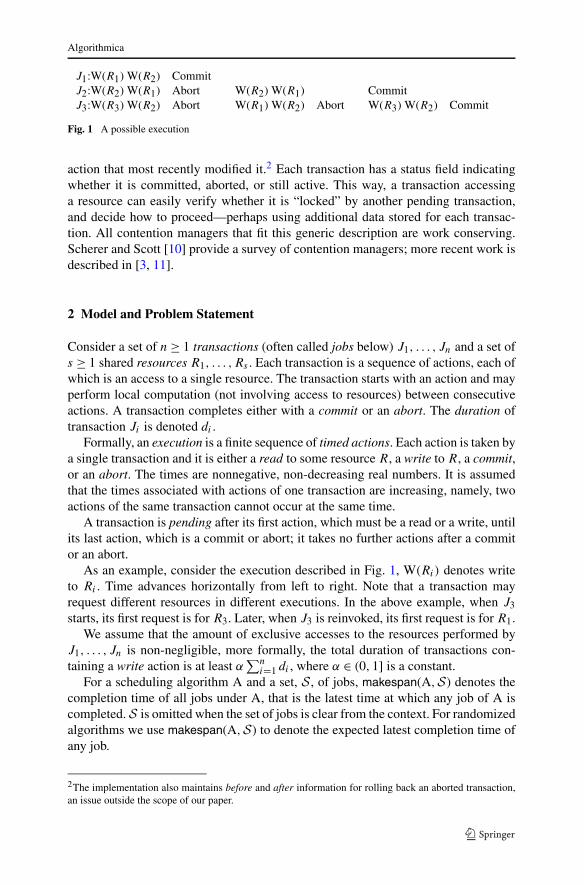
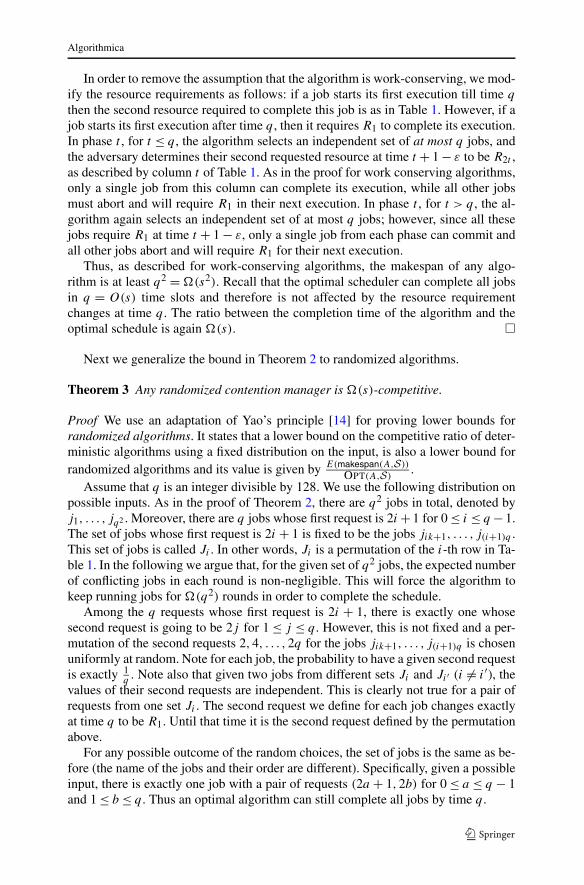
J1:W(R1) W(R2) CommitJ2:W(R2) W(R1) Abort W(R2) W(R1) CommitJ3:W(R3) W(R2) Abort W(R1) W(R2) Abort W(R3) W(R2) Commit

Fig. 1 A possible execution

action that most recently modified it.2 Each transaction has a status field indicatingwhether it is committed, aborted, or still active. This way, a transaction accessinga resource can easily verify whether it is “locked” by another pending transaction,and decide how to proceed—perhaps using additional data stored for each transac-tion. All contention managers that fit this generic description are work conserving.Scherer and Scott [10] provide a survey of contention managers; more recent work isdescribed in [3, 11].

2 Model and Problem Statement

Consider a set of n ≥ 1 transactions (often called jobs below) J1, . . . , Jn and a set ofs ≥ 1 shared resources R1, . . . ,Rs . Each transaction is a sequence of actions, each ofwhich is an access to a single resource. The transaction starts with an action and mayperform local computation (not involving access to resources) between consecutiveactions. A transaction completes either with a commit or an abort. The duration oftransaction Ji is denoted di .

Formally, an execution is a finite sequence of timed actions. Each action is taken bya single transaction and it is either a read to some resource R, a write to R, a commit,or an abort. The times are nonnegative, non-decreasing real numbers. It is assumedthat the times associated with actions of one transaction are increasing, namely, twoactions of the same transaction cannot occur at the same time.

A transaction is pending after its first action, which must be a read or a write, untilits last action, which is a commit or abort; it takes no further actions after a commitor an abort.

As an example, consider the execution described in Fig. 1, W(Ri) denotes writeto Ri . Time advances horizontally from left to right. Note that a transaction mayrequest different resources in different executions. In the above example, when J3starts, its first request is for R3. Later, when J3 is reinvoked, its first request is for R1.

We assume that the amount of exclusive accesses to the resources performed byJ1, . . . , Jn is non-negligible, more formally, the total duration of transactions con-taining a write action is at least α

∑ni=1 di , where α ∈ (0,1] is a constant.

For a scheduling algorithm A and a set, S , of jobs, makespan(A,S) denotes thecompletion time of all jobs under A, that is the latest time at which any job of A iscompleted. S is omitted when the set of jobs is clear from the context. For randomizedalgorithms we use makespan(A,S) to denote the expected latest completion time ofany job.

2The implementation also maintains before and after information for rolling back an aborted transaction,an issue outside the scope of our paper.

Algorithmica

A transaction may access different resources in different invocations, when it isre-invoked after an abort; this is natural, for example, in the context of a transactionthat access resources according to their functionality, e.g., “the last node in a list”,rather than their address. While the online algorithm does not know these accessesuntil they occur, an optimal offline algorithm, denoted OPT, knows the sequence ofaccesses of the transaction to resources in each execution.

We make the following simple observation on the decisions of OPT.

Claim 1 There is an algorithm OPT that achieves the minimum makespan and sched-ules each job exactly once.

Proof Any execution with minimum makespan can be modified so as to remove allpartial executions. Clearly, this does not increase the makespan and provides theabove property. �

3 The Greedy Algorithm Has O(s)-Competitive Makespan

The greedy algorithm GREEDY, suggested in [3], schedules a maximal independentset of jobs (i.e., jobs that are non-conflicting over their first-requested resources).When a set of jobs is running, and some of these jobs are conflicting over some re-source, Rj , GREEDY grants access to the “oldest” job among them, io. If io needs toperform write, then all other jobs are aborted; if it performs read, any other “reader”can access Rj too. The algorithm guarantees the pending commit property: at anytime in the execution, at least one job (the oldest) is guaranteed to complete its exe-cution without being aborted.

Theorem 1 GREEDY is O(s)-competitive.

Proof Consider the sequence of idle time intervals, I1, . . . , Ik in which no job isrunning under GREEDY, and the sequence of time intervals I ′

1, . . . , I′� in which no

job is running under OPT. We first prove that there exists an optimal schedule inwhich the total idle time is at least the total idle time of GREEDY. Formally,

Claim 2∑k

j=1 |Ij | ≤ ∑�j=1 |I ′

j |.

Proof By definition, GREEDY is idle at a certain time only after completing all jobsavailable at that time. Let I1 = [t1, t2]; this implies that during time interval [0, t1],GREEDY is busy processing some set of jobs S. The processing of S is completed attime t1, and the next job is released at time t2. There exists an optimal schedule thatcompletes the (sub)instance S at time at most t1, is idle until t2, and possibly has ad-ditional idle intervals during [0, t1]. Such an optimal schedule exists, since GREEDY

completes all jobs in S by time t1 and no job is available before time t2. Since we areinterested in a schedule which minimizes the makespan, it is even possible to simplyadopt the schedule of GREEDY without violating the optimality of the schedule.

Therefore, there exists an optimal schedule with total idle time at least t2 − t1 =|I1| till time t2. Continuing the same way, for each prefix of idle intervals, we get

Algorithmica

that for any j,1 ≤ j ≤ k, there exists an optimal schedule with total idle time at least∑j

i=1 |Ii | till the end of Ij . In particular, for j = k this gives the statement of theclaim. �

By assumption, a job accesses at least one resource at any time during its exe-cution. Consider the set of write actions of all transactions. If s + 1 jobs or moreare running concurrently, the pigeonhole principle implies that at least two of themare accessing the same resource. Thus, at least one out of s + 1 writing jobs will beaborted. Claim 1 implies that no job is aborted in an execution of OPT, implying thatat most s writing jobs are running concurrently during time intervals that are not idleunder OPT, that is, outside I ′

1, . . . , I′�. Thus, the makespan of OPT satisfies:

makespan(OPT) ≥�∑

j=1

|I ′j | +

α∑n

i=1 di

s.

On the other hand, whenever GREEDY is not idle, at least one of the jobs that areprocessed will be completed. Hence, the makespan of GREEDY satisfies:

makespan(GREEDY) ≤k∑

j=1

|Ij | +n∑

i=1

di.

The theorem follows. �

We remark that the same proof holds for any work conserving contention managerthat guarantees the pending commit property.

4 �(s) Lower Bounds for Contention Managers

4.1 A Lower Bound for Fixed First-Request

In the following, we give a matching lower bound to the upper bound derived inSect. 3 for GREEDY.

We first prove the lower bound for work conserving contention manager, and thenextend it to any deterministic algorithm. The proof constructs a set of jobs and re-quests, for which a non-clairvoyant manager obtains makespan �(s2), while themakespan achieved by a clairvoyant manager is O(s). Intuitively, the idea is to haveO(s) sets, each with O(s) unit-length jobs. In every set, all jobs ask for the same firstresource. Thus, only one job from each set can start in each time slot. A clairvoyantcontention manager, which knows the whole set of resources to be required by eachjob, can complete a set of O(s) non-conflicting jobs in each time slot, resulting inmakespan O(s). However, for any contention manager, and for each set of jobs se-lected to be executed simultaneously, an adversary can determine an identical secondrequested resource, enforcing all but one of the jobs to abort. This yields makespanO(s2). The details follow.

Algorithmica

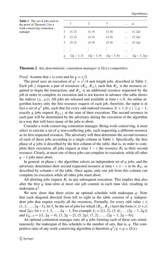
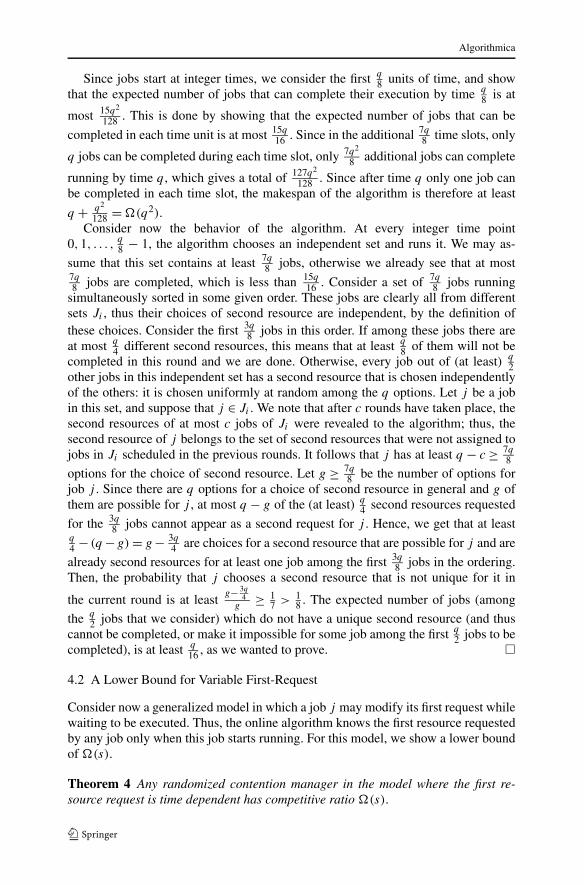
Table 1 The set of jobs used inthe proof of Theorem 2 for awork-conserving contentionmanager.

1 2 3 . . . q

1 (1,2) (1,4) (1,6) . . . (1,2q)

2 (3,2) (3,4) (3,6) . . . (3,2q)

3 (5,2) (5,4) (5,6) . . . (5,2q)

.

.

....

.

.

.... . . .

.

.

.

q (2q − 1,2) (2q − 1,4) (2q − 1,6) . . . (2q − 1,2q)

Theorem 2 Any deterministic contention manager is �(s)-competitive.

Proof Assume that s is even and let q = s/2.The proof uses an execution of q2 = s2/4 unit length jobs, described in Table 1:

Each job j requests a pair of resources (Rj1 ,Rj2), such that Rj1 is the resource re-quired to begin the transaction, and Rj2 is an additional resource requested by thejob in order to complete its execution and is not known in advance (the table showsthe indices (j1, j2)). All jobs are released and available at time t = 0. An online al-gorithm knows only the first resource request of each job, therefore, the input is infact a set of q2 jobs, such that for every odd-indexed resource 2i + 1,0 ≤ i ≤ q − 1,exactly q jobs request R2i+1 at the start of their execution. The second resource ineach pair will be determined by the adversary during the execution of the algorithmin a way that will force many of the jobs to abort.

Consider a work-conserving contention manager. Being work-conserving, it mustselect to execute a set of q non-conflicting jobs, each requesting a different resourceas its first requested resource. The adversary will then determine the second resourceof each of these jobs according to a single column in Table 1. Specifically, the firstphase of q jobs is described by the first column of the table, that is, in order to com-plete their execution, all jobs request at time 1 − ε the resource R2 as their secondresource. Clearly, at most one of these jobs can complete its execution, while all otherq − 1 jobs must abort.

In general, in phase t , the algorithm selects an independent set of q jobs, and theadversary determines their second requested resource at time t + 1 − ε to be R2t , asdescribed by column t of the table. Once again, only one job from this column cancomplete its execution while all other jobs must abort.

All aborting jobs request R1 in any subsequent execution. This implies that alsoafter the first q time-slots at most one job commit in each time slot, resulting inmakespan q2.

We now show that there exists an optimal schedule with makespan q: Notethat each diagonal directed from left to right in the table consists of q indepen-dent jobs that require exactly all the resources. Formally, for every odd value z ∈{1,3, . . . ,2q−1}, let Iz be the set of jobs for which (Rj1,Rj2) have the form (r, (r+z)

mod 2q), for r = 1,3, . . . ,2q − 1. For example I1 = {(1,2), (3,4), . . . (2q − 1,2q)}and I2q−5 = {(1,2q − 4), (3,2q − 2), (5,2q), (7,2), . . . , (2q − 1,2q − 6)}.

An optimal contention manager runs all q jobs forming each of these sets simul-taneously; the makespan of this schedule is the number of sets, that is, q . The com-petitive ratio of any work-conserving algorithm is therefore q2/q = q = �(s).

Algorithmica

In order to remove the assumption that the algorithm is work-conserving, we mod-ify the resource requirements as follows: if a job starts its first execution till time q

then the second resource required to complete this job is as in Table 1. However, if ajob starts its first execution after time q , then it requires R1 to complete its execution.In phase t , for t ≤ q , the algorithm selects an independent set of at most q jobs, andthe adversary determines their second requested resource at time t + 1 − ε to be R2t ,as described by column t of Table 1. As in the proof for work conserving algorithms,only a single job from this column can complete its execution, while all other jobsmust abort and will require R1 in their next execution. In phase t , for t > q , the al-gorithm again selects an independent set of at most q jobs; however, since all thesejobs require R1 at time t + 1 − ε, only a single job from each phase can commit andall other jobs abort and will require R1 for their next execution.

Thus, as described for work-conserving algorithms, the makespan of any algo-rithm is at least q2 = �(s2). Recall that the optimal scheduler can complete all jobsin q = O(s) time slots and therefore is not affected by the resource requirementchanges at time q . The ratio between the completion time of the algorithm and theoptimal schedule is again �(s). �

Next we generalize the bound in Theorem 2 to randomized algorithms.

Theorem 3 Any randomized contention manager is �(s)-competitive.

Proof We use an adaptation of Yao’s principle [14] for proving lower bounds forrandomized algorithms. It states that a lower bound on the competitive ratio of deter-ministic algorithms using a fixed distribution on the input, is also a lower bound forrandomized algorithms and its value is given by E(makespan(A,S))

OPT(A,S).

Assume that q is an integer divisible by 128. We use the following distribution onpossible inputs. As in the proof of Theorem 2, there are q2 jobs in total, denoted byj1, . . . , jq2 . Moreover, there are q jobs whose first request is 2i + 1 for 0 ≤ i ≤ q − 1.The set of jobs whose first request is 2i + 1 is fixed to be the jobs jik+1, . . . , j(i+1)q .This set of jobs is called Ji . In other words, Ji is a permutation of the i-th row in Ta-ble 1. In the following we argue that, for the given set of q2 jobs, the expected numberof conflicting jobs in each round is non-negligible. This will force the algorithm tokeep running jobs for �(q2) rounds in order to complete the schedule.

Among the q requests whose first request is 2i + 1, there is exactly one whosesecond request is going to be 2j for 1 ≤ j ≤ q . However, this is not fixed and a per-mutation of the second requests 2,4, . . . ,2q for the jobs jik+1, . . . , j(i+1)q is chosenuniformly at random. Note for each job, the probability to have a given second requestis exactly 1

q. Note also that given two jobs from different sets Ji and Ji′ (i �= i′), the

values of their second requests are independent. This is clearly not true for a pair ofrequests from one set Ji . The second request we define for each job changes exactlyat time q to be R1. Until that time it is the second request defined by the permutationabove.

For any possible outcome of the random choices, the set of jobs is the same as be-fore (the name of the jobs and their order are different). Specifically, given a possibleinput, there is exactly one job with a pair of requests (2a + 1,2b) for 0 ≤ a ≤ q − 1and 1 ≤ b ≤ q . Thus an optimal algorithm can still complete all jobs by time q .

Algorithmica

Since jobs start at integer times, we consider the first q8 units of time, and show

that the expected number of jobs that can complete their execution by time q8 is at

most 15q2

128 . This is done by showing that the expected number of jobs that can be

completed in each time unit is at most 15q16 . Since in the additional 7q

8 time slots, only

q jobs can be completed during each time slot, only 7q2

8 additional jobs can complete

running by time q , which gives a total of 127q2

128 . Since after time q only one job canbe completed in each time slot, the makespan of the algorithm is therefore at least

q + q2

128 = �(q2).Consider now the behavior of the algorithm. At every integer time point

0,1, . . . ,q8 − 1, the algorithm chooses an independent set and runs it. We may as-

sume that this set contains at least 7q8 jobs, otherwise we already see that at most

7q8 jobs are completed, which is less than 15q

16 . Consider a set of 7q8 jobs running

simultaneously sorted in some given order. These jobs are clearly all from differentsets Ji , thus their choices of second resource are independent, by the definition ofthese choices. Consider the first 3q

8 jobs in this order. If among these jobs there areat most q

4 different second resources, this means that at least q8 of them will not be

completed in this round and we are done. Otherwise, every job out of (at least) q2

other jobs in this independent set has a second resource that is chosen independentlyof the others: it is chosen uniformly at random among the q options. Let j be a jobin this set, and suppose that j ∈ Ji . We note that after c rounds have taken place, thesecond resources of at most c jobs of Ji were revealed to the algorithm; thus, thesecond resource of j belongs to the set of second resources that were not assigned tojobs in Ji scheduled in the previous rounds. It follows that j has at least q − c ≥ 7q

8

options for the choice of second resource. Let g ≥ 7q8 be the number of options for

job j . Since there are q options for a choice of second resource in general and g ofthem are possible for j , at most q − g of the (at least) q

4 second resources requested

for the 3q8 jobs cannot appear as a second request for j . Hence, we get that at least

q4 − (q −g) = g − 3q

4 are choices for a second resource that are possible for j and are

already second resources for at least one job among the first 3q8 jobs in the ordering.

Then, the probability that j chooses a second resource that is not unique for it in

the current round is at leastg− 3q

4g

≥ 17 > 1

8 . The expected number of jobs (among

the q2 jobs that we consider) which do not have a unique second resource (and thus

cannot be completed, or make it impossible for some job among the first q2 jobs to be

completed), is at least q16 , as we wanted to prove. �

4.2 A Lower Bound for Variable First-Request

Consider now a generalized model in which a job j may modify its first request whilewaiting to be executed. Thus, the online algorithm knows the first resource requestedby any job only when this job starts running. For this model, we show a lower boundof �(s).

Theorem 4 Any randomized contention manager in the model where the first re-source request is time dependent has competitive ratio �(s).

Algorithmica

Proof We first prove a lower bound of �(s) for an arbitrary online deterministicalgorithm, and then show how to adapt it to randomized algorithms. Let s′ = �s/2�.

In our execution, each job will have a single request for a resource. It reveals theinformation regarding the resources it is going to need each time it restarts. Thus, theresource requests are time dependent.

At first, there are 2s′ sets of unit-length jobs A1, . . . ,A2s′ . Each set contains 2s′jobs, where all jobs in one set Ai initially request resource i. For some of the jobsthis is changed later on. Consider the situation after s′ time units.

We define an offline contention manager OFF. Partition each set Ai into Bi andCi . The set Ci contains all jobs in Ai that the algorithm completes by time s′. Addadditional jobs from Ai to Ci until |Ci | = s′. Let Bi = Ai − Ci . OFF runs the jobs ofBi during time units 1,2, . . . , s′. Since each set Bi requested a different resource, attime s′, OFF completes all these jobs. However, the online algorithm did not run anyof these jobs yet. Starting at time s′, the jobs in B2,B3, . . . ,Bs request resource R1when they start running. Thus, all waiting requests need to use the same resource, andthe online algorithm needs 2s′2 additional time units to complete them. In contrast,OFF needs only s′ additional time units, since it can now run the Ci jobs for alli in s′ time units in parallel. We get that the algorithm completes all jobs at times′ + 2s′2, whereas OFF completes all jobs by time 2s′. This gives a lower bound of12 + s′ = �(s).

Assume now that the algorithm is randomized. Instead of defining Ci as before,let Ci be the set of s′ elements of Ai with the highest probability to be run by thealgorithm and complete by time s′. Let Bi = Ai − Ci , i.e., the jobs with smallestprobabilities to terminate successfully by time s′. As in the deterministic case, OFF

runs all jobs of all Bi until time s′ and afterward all jobs of Ci . Also, all jobs of Bi

request only resource 1 if they are run starting from time s′ or later.Let Xi (respectively Yi ) be the number of elements of Bi (Ci ) that have been

completed by the algorithm by time s′. It holds that E(Xi) ≤ s′2 . To see this, we use

the linearity of expectation and get E(Xi) ≤ E(Yi) and since Xi + Yi ≤ s′ we haveE(Xi) + E(Yi) ≤ s′. Thus, the expected number of elements from all Bi ’s that are

still waiting to be scheduled by the algorithm is at least 2s′22 = s′2. It follows that

the expected makespan is at least s′ + s′2, and we get a lower bound of �(s) for therandomized case as well. �

We remark that GREEDY is O(s)-competitive also in this generalized model. Theproof of Theorem 1 makes no assumption on the identities of the requested resources,i.e., a job may modify its resource request as long as it has not started running; also,if a job was aborted and then restarted, it may initially ask for one resource, and latermodify its request.

5 Handling Failures

Consider a system in which jobs may fail; if a job j running at time t fails, the con-tention manager subsequently needs to restart the execution of j . Following Guer-raoui et al. [4] we assume that a job may fail at most k times, for some k ≥ 1; after

Algorithmica

a failure, the job is restarted. Indeed, for any job j , GREEDY may run j almost tocompletion k times, and then restart its execution due to a failure. This stretches theprocessing time of j to (k +1)dj . In contrast, an optimal offline algorithm may avoidthe execution of a job j when j may fail. This implies:

Theorem 5 If each job may fail at most k times, then GREEDY is O(ks)-competitive.

5.1 Lower Bounds

For this model, we show a lower bound of �(ks) for any deterministic algorithm. Thelower bound is obtained by constructing a job sequence in which failure occurs, foreach of the jobs, shortly before the job completes its execution. Since each job failsk times, the deterministic online algorithm is forced to start the execution of each jobk times.

Theorem 6 Assume that the first request of a job for a resource is time dependent,and each job may fail at most k times, for some k ≥ 1, then any deterministic con-tention manager has competitive ratio �(ks).

Proof Define the sets Ai , Bi and Ci as in the proof of Theorem 4. The sequenceis the same until time 2s′ (= 2�s/2�) at which OFF completes all jobs. After thistime, we define failure times as follows. Consider the schedule of the algorithm. Ifa running job already failed k times then it is not interrupted; otherwise, it fails justbefore completion. Thus, all jobs except for at most 2s′2 + s′ fail exactly k times.Since the failure of any job occurs almost upon completion, the remaining 2s′2 − s′jobs are completed only after (k + 1)(2s′2 − s′) additional times units. We get a totalof (k + 1)(2s′2 − s′) + 2s′ time slots, and a lower bound of �(ks). �

We also obtain a lower bound also for randomized algorithms.

Theorem 7 Assume that the first request of a job for a resource is time dependent,and each job may fail at most k times, for some k ≥ 1, then any (deterministic orrandomized) contention manager has competitive ratio �(max{s, k}).

Proof Assume that k ≥ 5, otherwise the deterministic bounds can be applied. A lowerbound of �(s) follows from Theorem 4. To prove a lower bound of k consider aninput with two jobs j1 and j2, each having (a different) one of the two sets of failuretimes: {1, 3

2 ,2, 52 , . . . , k+1

2 } or { 12 ,1,2, 5

2 , . . . , k+12 }. Both sets contain all multiples of

12 (up to and including k+1

2 ) except one such number: the first set does not contain12 whereas the second one does not contain 3

2 . Assume that s = 1, thus, the issue ofresources may be ignored. An offline algorithm can run the job with the first failuretimes sequence at time 0, until time 1, and the other job at time 1, until time 2.

Consider an online algorithm. Let p1 be the probability that job j1 is running justbefore time 1

2 and p2 that j2 is running. We have p1 + p2 ≤ 1 (since it may be thecase that no job is running). If p1 ≤ p2, we assign the first failure times sequence toj1 and the second one to j2, and otherwise we do the opposite assignment. The only

Algorithmica

way that all jobs are completed by time 2, is that some job is completed by time 1, andthus this job needs to be running just before time 1

2 , and not interrupted at time 12 . The

probability for that is p1 in the first case and p2 in the second case. However, in thefirst case p1 ≤ 1

2 and in the second case p2 ≤ 12 , so with probability at least 1

2 , at leastone job can run to completion only after time k+1

2 . Thus, the expected completiontime is at least 1

2 · 2 + 12 · ( k+1

2 + 1) = �(k). �

Next we describe a randomized algorithm that matches this bound within a loga-rithmic factor for the case where all jobs require unit processing time. We start with adescription of a centralized scheduler, and later explain how to make it decentralized.

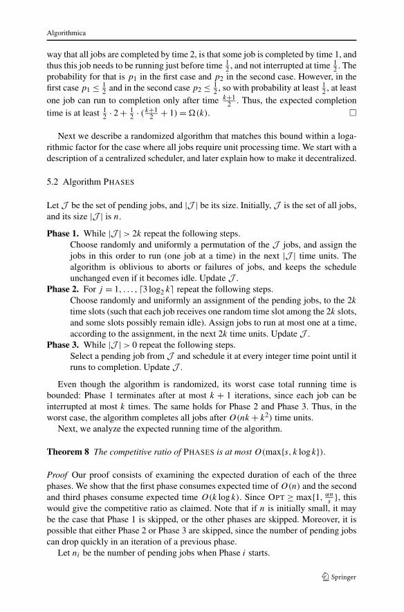
5.2 Algorithm PHASES

Let J be the set of pending jobs, and |J | be its size. Initially, J is the set of all jobs,and its size |J | is n.

Phase 1. While |J | > 2k repeat the following steps.Choose randomly and uniformly a permutation of the J jobs, and assign thejobs in this order to run (one job at a time) in the next |J | time units. Thealgorithm is oblivious to aborts or failures of jobs, and keeps the scheduleunchanged even if it becomes idle. Update J .

Phase 2. For j = 1, . . . , 3 log2 k repeat the following steps.Choose randomly and uniformly an assignment of the pending jobs, to the 2k

time slots (such that each job receives one random time slot among the 2k slots,and some slots possibly remain idle). Assign jobs to run at most one at a time,according to the assignment, in the next 2k time units. Update J .

Phase 3. While |J | > 0 repeat the following steps.Select a pending job from J and schedule it at every integer time point until itruns to completion. Update J .

Even though the algorithm is randomized, its worst case total running time isbounded: Phase 1 terminates after at most k + 1 iterations, since each job can beinterrupted at most k times. The same holds for Phase 2 and Phase 3. Thus, in theworst case, the algorithm completes all jobs after O(nk + k2) time units.

Next, we analyze the expected running time of the algorithm.

Theorem 8 The competitive ratio of PHASES is at most O(max{s, k logk}).

Proof Our proof consists of examining the expected duration of each of the threephases. We show that the first phase consumes expected time of O(n) and the secondand third phases consume expected time O(k logk). Since OPT ≥ max{1, αn

s}, this

would give the competitive ratio as claimed. Note that if n is initially small, it maybe the case that Phase 1 is skipped, or the other phases are skipped. Moreover, it ispossible that either Phase 2 or Phase 3 are skipped, since the number of pending jobscan drop quickly in an iteration of a previous phase.

Let ni be the number of pending jobs when Phase i starts.

Algorithmica

Consider Phase 1. Let Xi be a random variable which denotes the length of iter-ation i of this phase; clearly, X1 = n1 = n. We claim that E(Xi) ≤ Xi−1

2 for i ≥ 2.Each job has equal probability to be assigned to each time slot, and since n > 2k

during this phase, the probability of a job to run to completion during iteration i − 1is at least 1

2 . This holds since there are at most k times where a job may fail whilerunning, so there are at least k options to schedule it so that it does not fail. Sincethis holds for any value of Xi , and due to linearity of expectation, we conclude thatE(Xi) ≤ E(Xi−1)

2 . By induction, E(Xi) ≤ 12i−1 n1 = 1

2i−1 n. Let t be the number of it-erations in Phase 1, which is at most k + 1. Therefore, the expected length of Phase 1is at most

∑ti=1 E(Xi) = ∑t

i=11

2i−1 n ≤ 2n.Consider Phase 2. Since n2 ≤ 2k, each iteration admits an assignment of all jobs to

time slots. Consider a specific job scheduled in an iteration. This job may be assignedto any of the 2k time slots starting at integer times with equal probability. However,out of these slots, at most k can prevent a successful completion of the job. Thus, thejob is completed in a given iteration with probability at least 1

2 .We next bound (from above) the probability that the algorithm reaches Phase 3.

The probability of a given job to be pending, even after 3 log2 k iterations ofPhase 2, is at most ( 1

2 )3 log2 k ≤ 1k3 . Using the sum of probabilities as an upper bound,

the probability that at least one job is left for Phase 3 is at most n2k3 ≤ 2k

k3 = 2k2 . Thus,

with probability at most 1 − 2k2 , the algorithm does not reach Phase 3, and the overall

running time for Phases 2 and 3 is at most 2k · 3 log2 k.Phase 3 lasts at most k + 1 times units for every job, and thus takes at most

n3(k + 1) ≤ 2k(k + 1) time units. This happens with probability at most 2k2 , and

gives expected additional time of at most 4(k+1)k

< 5. We get for Phases 2 and 3 anexpected total running time of O(k log k), which completes the proof. �

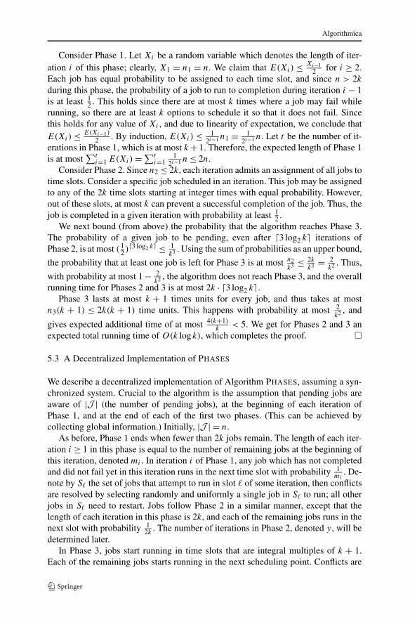
5.3 A Decentralized Implementation of PHASES

We describe a decentralized implementation of Algorithm PHASES, assuming a syn-chronized system. Crucial to the algorithm is the assumption that pending jobs areaware of |J | (the number of pending jobs), at the beginning of each iteration ofPhase 1, and at the end of each of the first two phases. (This can be achieved bycollecting global information.) Initially, |J | = n.

As before, Phase 1 ends when fewer than 2k jobs remain. The length of each iter-ation i ≥ 1 in this phase is equal to the number of remaining jobs at the beginning ofthis iteration, denoted mi . In iteration i of Phase 1, any job which has not completedand did not fail yet in this iteration runs in the next time slot with probability 1

mi. De-

note by S� the set of jobs that attempt to run in slot � of some iteration, then conflictsare resolved by selecting randomly and uniformly a single job in S� to run; all otherjobs in S� need to restart. Jobs follow Phase 2 in a similar manner, except that thelength of each iteration in this phase is 2k, and each of the remaining jobs runs in thenext slot with probability 1

2k. The number of iterations in Phase 2, denoted y, will be

determined later.In Phase 3, jobs start running in time slots that are integral multiples of k + 1.

Each of the remaining jobs starts running in the next scheduling point. Conflicts are

Algorithmica

Initially, i = 0.

Phase 1. While |J | > 2k repeat the following steps.i = i + 1mi = |J |For � = 1 to mi doS� = ∅For any j ∈J do

If j did not fail yet in iteration i then with probability 1/mi S� = S� ∪ {j}.If there are conflicting jobs in S�, select randomly and uniformly one job j ∈ S�

to run in slot �, and S� = {j}.J = J \ S�

Phase 2. For i = 1 to y doFor � = 1 to 2k do

S� = ∅For any j ∈J do

If j did not fail yet in iteration i then with probability 1/2k S� = S� ∪ {j}.If there are conflicting jobs in S�, select randomly and uniformly one job j ∈ S�

to run in slot �, and S� = {j}.J = J \ S�

Phase 3. � = 0While |J | > 0 do

S� = ∅For any j ∈ J do S� = S� ∪ {j}.If there are conflicting jobs in S�, run the oldest job jo ∈ S� in the nextk + 1 slots, and S� = {jo}.

J =J \ S�

� = � + k + 1

Fig. 2 Algorithm DECENTRALIZED PHASES

resolved by selecting the oldest job to run in the next k + 1 slots, while the remainingjobs need to restart.

The pseudocode of the algorithm appears in Fig. 2.We next analyze the algorithm and show that it is a decentralized implementation

of algorithm PHASES, where the expected running time increases by a constant factor.

Theorem 9 The expected running time of the decentralized implementation ofPHASES is O(n + k logk).

Proof We show that the expected length of Phase 1 is O(n), while the expected lengthof Phases 2 and 3 is O(k log k).

Consider Phase 1. Suppose that some job J� tries to run in slot j of iteration i.The probability that no other job attempts to run in this slot is at least

(

1 − 1

mi

)mi−1

≥ mi

mi − 1e−2 ≥ e−2. (1)

Algorithmica

If job J� runs alone in some slot in iteration i and does not fail, then J� completes inthis iteration. To lower bound the probability that job J� completes in iteration i, letGoodi denote the set of (at least) mi − k time slots that are good for J� in iteration i,i.e., if J� runs in any of these slots then it does not fail. Also, let Ai

j be the event “Initeration i, job J� runs for the first time in slot j , and conflicts with no other job inthis slot,” then the probability that J� completes in iteration i is at least

∑

j∈Goodi

Prob(Aij )

≥∑

j∈Goodi

(

1 − 1

mi

)j−1

· 1

mi

· 1

e2

≥mi∑

j=k+1

(

1 − 1

mi

)j−1 1

e2mi

=(

1 − 1

mi

)k 1 − (1 − 1mi

)mi−k

e2

≥(

1 − 1

mi

)mi/2 1

e2

(

1 −(

1 − 1

mi

)mi/2)

since k ≤ mi/2

≥ 1

e3

(

1 − 1√e

)

since e−1 ≤(

1 − 1

mi

)mi/2

≤ e−1/2.

The first inequality follows from (1), and the second from the fact that, for thelower bound, we may assume that Goodi are the last (mi − k) slots in iteration i.Letting δ = e−3(1 − 1/

√e), we get that

E[Xi] ≤ (1 − δ)E[Xi−1],where Xi is a random variable denoting the length of iteration i of Phase 1 (as inthe analysis of Phase 1 in algorithm PHASES). It follows that the expected length ofPhase 1 is bounded by

∑i≥1(1 − δ)i−1n = n

δ.

For Phase 2, we set the number of iterations to be

y = log(2(k + 1)/ log k)/ log(1/(1 − δ)),

and get that its length is 2k · y = O(k logk).For Phase 3, recall that the number of remaining jobs at the beginning of Phase 2

is bounded by 2k; the probability that a job that started Phase 2 does not completeby the end of the phase is at most (1 − δ)y <

log k2(k+1)

. Since each of the jobs startingPhase 3 gets (k + 1) time slots, the expected length of this phase is at most (1 − δ)y ·2k(k + 1) = O(k logk). This completes the proof. �

In the decentralized implementation of PHASES, the worst case length of Phase 1 isunbounded. The following adaptation of the algorithm results in bounding the length

Algorithmica

of Phase 1 by O(nk). When the phase reaches iteration z = log(k/2)/ log(1/1 − δ),every remaining job starts running in the next time slot. Conflicts are resolved asbefore, by random selection of one job in the conflict set. Clearly, this implies thatin the next (k + 1)n time units all jobs complete. Note that, with this modification,the expected length of Phase 1 is at most O(n) + ∑n

�=1(1 − δ)z(k + 1). The leftterm reflects the expected running time of the original decentralized algorithm, andthe second term gives the expected number of slots used after iteration z. Here, weconsider only jobs which have not completed by iteration z and assign to each ofthese jobs (k + 1) time slots. Since

∑n�=1(1 − δ)z(k + 1) < 3n, the expected running

time remains O(n). The lengths of the other two phases are bounded.

6 Discussion

We take the perspective of non-clairvoyant scheduling to analyze the behavior oftransactional contention managers. Our framework can be extended to models notconsidered here such as the case where the amount of exclusive accesses to the re-sources is negligible, i.e., when there are many read-only jobs.

Another problem that remains open is the optimality of work-conserving con-tention managers. The lower bound of �(s) presented in Theorem 2 holds fornon work-conserving contention managers; however, for work-conserving contentionmanagers the lower bound is suitable also for more powerful systems in which theresource requests of a transaction do not change when it is re-executed.

The analysis of Algorithm PHASES hinges on the fact that the probability of ajob trying to execute in a phase depends on the number of pending jobs. Scherer andScott [10] describe a practical randomized contention manager that flips a coin tochoose between aborting the other transaction and waiting for a random time. Ouranalysis suggests that this contention manager can be more effective by biasing thecoin in a way that depends on (at least) an estimate of the number of jobs waiting tobe executed.

Another interesting avenue for further research is to evaluate other complexitymeasures, in particular, those that evaluate the guarantees provided for each individ-ual transaction, like the average response or waiting time or the average punishment.

Acknowledgements We would like to thank Rachid Guerraoui, Michał Kapałka and Bastian Pochonfor helpful discussions, and the anonymous referees for their comments.

References

1. Borodin, A., El-Yaniv, R.: Online Computation and Competitive Analysis. Cambridge UniversityPress, Cambridge (1998)

2. Edmonds, J., Chinn, D.D., Brecht, T., Deng, X.: Non-clairvoyant multiprocessor scheduling of jobswith changing execution characteristics. J. Sched. 6(3), 231–250 (2003)

3. Guerraoui, R., Herlihy, M., Pochon, B.: Toward a theory of transactional contention management. In:Proceedings of the 24th Annual ACM Symposium on Principles of Distributed Computing (PODC),pp. 258–264 (2005)

Algorithmica

4. Guerraoui, R., Herlihy, M., Kapałka, M., Pochon, B.: Robust contention management in soft-ware transactional memory. In: Synchronization and Concurrency in Object-Oriented Lan-guages (SCOOL). Workshop, in Conjunction with OOPSLA (2005). http://urresearch.rochester.edu/handle/1802/2103

5. Herlihy, M., Luchangco, V., Moir, M., Scherer III, W.N.: Software transactional memory for dynamic-sized data structures. In: Proceedings of the 22nd Annual ACM Symposium on Principles of Distrib-uted Computing (PODC), pp. 92–101 (2003)

6. Irani, S., Leung, V.: Scheduling with conflicts, and applications to traffic signal control. In: Proceed-ings of the 7th Annual ACM-SIAM Symposium on Discrete Algorithms (SODA), pp. 85–94 (1996)

7. Kalyanasundaram, B., Pruhs, K.R.: Fault-tolerant scheduling. SIAM J. Comput. 34(3), 697–719(2005)

8. Motwani, R., Phillips, S., Torng, E.: Non-clairvoyant scheduling. Theor. Comput. Sci. 130(1), 17–47(1994)

9. Rosenkrantz, D.J., Stearns, R.E., Lewis II, P.M.: System level concurrency control for distributeddatabase systems. ACM Trans. Database Syst. 3(2), 178–198 (1978)

10. Scherer III, W.N., Scott, M.: Contention management in dynamic software transactional memory. In:PODC Workshop on Concurrency and Synchronization in Java Programs, pp. 70–79 (2004)

11. Scherer III, W.N., Scott, M.: Advanced contention management for dynamic software transactionalmemory. In: Proceedings of the 24th Annual ACM Symposium on Principles of Distributed Comput-ing (PODC), pp. 240–248 (2005)

12. Silberschatz, A., Galvin, P.: Operating Systems Concepts, 5th edn. Wiley, New York (1999)13. Vossen, G., Weikum, G.: Transactional Information Systems. Morgan Kaufmann, San Mateo (2001)14. Yao, A.C.C.: Probabilistic computations: towards a unified measure of complexity. In: Proc. 18th

Symp. Foundations of Computer Science (FOCS), pp. 222–227. IEEE (1977)