Algorithms On Continued And Multicontinued FractionsFranck Nielsen1E.N.S. LyonFrancefnielsen@ens.ens-lyon.fr under the direction ofPeter Kornerup2University of OdenseDenmarkAugust 12, 1993

1Visiting student from the E.N.S. Lyon.2Professor of Computer Science, Odense University, Odense.

Acknowledgments:I would like to thank S�ren Peter Johansen and Peter Kornerup who have helped me duringthis work and have improved considerably the quality of this rapport.That the topless towers be burntAnd men recall that face,Move gently if move you mustIn this lonely place.She thinks, part woman, three parts a child,That nobody looks her feetPractice a tinker shu�ePicked up on street.Like a long-legged y upon the streamHer mind moves upon silence.W.B. Yeats, "Longed-legged Fly"

Year - MCMXCIIIKeywords: Continued Fraction, Redundant representation, Lexicographic Continued Fraction, Arith-metic Unit, Fine grained Parallelism, On-line, Hypercube, Gray Code, Multicontinued Fraction.

AbstractWe introduce a continued fraction binary representation of the rationals, and several associated algorithmsfor computing certain functions on rationals exactly. This work follows the path taken by the previousworks done in that area and extends the notion of continued fraction to multicontinued fraction. Forthat purpose, we introduce the notion of generalized matrix. This work is composed of six parts. Webegin by a survey on the di�erent kinds of representation of numbers. We then describe and algorithmwhich compute ax+bcx+d for any x when both inputs and outputs are provided piecewise. We generalizethis algorithm to compute complex functions f(x1; : : : ; xn) = P1(x1;:::;xn)P2(x1;:::;xn) where P1(�) and P2(�) arepolynomial functions of n variables. In the remaining, we show how it is possible to mix various formatsof numbers (both for the input and output of numbers). Approximation of a real to a rational vector isinvestigated (Szekeres' algorithm)). A matrix representation of multicontinued fractions is introducedand we develop an algorithm based on that representation to compute quotient of polynomial functions.

Algorithms on Continued Fractions 1Contents1 Several Codings of Numbers and their Matrix Representations: 31.1 Continued Fraction CF: : : : : : : : : : : : : : : : : : : : : : : : : : : : : : : : : : : : : : 31.2 Redundant Continued Fraction: : : : : : : : : : : : : : : : : : : : : : : : : : : : : : : : : : 61.3 Continued Logarithmic Fraction: : : : : : : : : : : : : : : : : : : : : : : : : : : : : : : : : 81.4 LCF - Lexicographic Continued Fraction: : : : : : : : : : : : : : : : : : : : : : : : : : : : 101.5 Matrix Representation of Continued Fraction Expansion: : : : : : : : : : : : : : : : : : : 111.6 Radix Coding: : : : : : : : : : : : : : : : : : : : : : : : : : : : : : : : : : : : : : : : : : : 121.7 Redundant Binary Representation (RPQ): : : : : : : : : : : : : : : : : : : : : : : : : : : : 122 Computation of Functions of One Variable: 142.1 Notations and Introduction to the Problem: : : : : : : : : : : : : : : : : : : : : : : : : : : 142.2 Consuming Input Piecewise: : : : : : : : : : : : : : : : : : : : : : : : : : : : : : : : : : : : 162.3 Producing Output Piecewise: : : : : : : : : : : : : : : : : : : : : : : : : : : : : : : : : : : 183 Introduction to Generalized Matrices: 203.1 Consuming Input Piecewise: : : : : : : : : : : : : : : : : : : : : : : : : : : : : : : : : : : : 233.2 Another Way to Process Input: : : : : : : : : : : : : : : : : : : : : : : : : : : : : : : : : : 253.2.1 Analyze in Term of Matrices: : : : : : : : : : : : : : : : : : : : : : : : : : : : : : : 253.2.2 Using the Hypercube Structure: : : : : : : : : : : : : : : : : : : : : : : : : : : : : : 253.3 Shrinking the Computational Tree when an Input is Exhausted: : : : : : : : : : : : : : : : 263.4 The Output Condition: : : : : : : : : : : : : : : : : : : : : : : : : : : : : : : : : : : : : : 263.5 Changing the Format of Numbers: : : : : : : : : : : : : : : : : : : : : : : : : : : : : : : : 273.6 Computing the Tree-like Matrix Given a Function: : : : : : : : : : : : : : : : : : : : : : : 283.7 Analogy with the Hypercube Structure: : : : : : : : : : : : : : : : : : : : : : : : : : : : : 293.7.1 Construction of Gray Code: : : : : : : : : : : : : : : : : : : : : : : : : : : : : : : 313.7.2 Processing Input and Output in the Hypercube H: : : : : : : : : : : : : : : : : : : 313.7.3 The Butter y (./) Operation: : : : : : : : : : : : : : : : : : : : : : : : : : : : : : : 323.7.4 An example: f(x1; x2; x3) = x1+x2+x3x1x2x3 . : : : : : : : : : : : : : : : : : : : : : : : : : 343.7.5 Algorithm on the Hypercube: : : : : : : : : : : : : : : : : : : : : : : : : : : : : : : 354 An Algorithm Based on the Hypercube to Compute f(x1; : : : ; xn) = Pnum(x1;:::;xn)Pden(x1;:::;xn) : 374.1 The Decision Hypercube : : : : : : : : : : : : : : : : : : : : : : : : : : : : : : : : : : : : : 374.1.1 De�nition of the Decision Hypercube: : : : : : : : : : : : : : : : : : : : : : : : : : 384.1.2 Updating the Decision Hypercube when an Input is Performed: : : : : : : : : : : : 384.1.3 Updating the Decision Hypercube when an Output is Performed: : : : : : : : : : : 394.1.4 Updating the Index of m and M : : : : : : : : : : : : : : : : : : : : : : : : : : : : : 394.2 The Bit Level Algorithm: : : : : : : : : : : : : : : : : : : : : : : : : : : : : : : : : : : : : 404.2.1 General Principle: : : : : : : : : : : : : : : : : : : : : : : : : : : : : : : : : : : : : 42E.N.S. Lyon & Odense Universitet

Algorithms on Continued Fractions 24.2.2 Using the LCF Format: : : : : : : : : : : : : : : : : : : : : : : : : : : : : : : : : : : 424.2.3 Using the RPQ Format: : : : : : : : : : : : : : : : : : : : : : : : : : : : : : : : : : 425 The Szekeres Multidimensional Continued Fraction: 445.1 Best and Good Rational Approximation to a real: : : : : : : : : : : : : : : : : : : : : : : 445.2 Good and Best Rational Approximations of a real k-vector: : : : : : : : : : : : : : : : : : 445.3 Algorithm to Compute Approximations to a Real k-vector: : : : : : : : : : : : : : : : : : 445.4 Application of the Szekeres' Algorithm in the Computation of Y = F �X: : : : : : : : : 486 An Algorithm for Computing Functions On Variables Entered in MulticontinuedFractions Format: 526.1 De�nition of a k-multicontinued Fraction: : : : : : : : : : : : : : : : : : : : : : : : : : : : 536.2 Matrix Representation of a Multicontinued Fraction: : : : : : : : : : : : : : : : : : : : : : 546.3 Computing Functions of One Variable Entered in the MultiContinued Fraction Format: : 546.4 Computation of Functions of Several Variables Entered in the Multicontinued FractionFormat: : : : : : : : : : : : : : : : : : : : : : : : : : : : : : : : : : : : : : : : : : : : : : : 56A A Few Words About the Simplex 58B The MCF-Simulator program: 60B.1 The type of functions allowed: : : : : : : : : : : : : : : : : : : : : : : : : : : : : : : : : : : 60B.2 A session with MCF-Simulator: : : : : : : : : : : : : : : : : : : : : : : : : : : : : : : : : 60B.3 Description of the input �le: : : : : : : : : : : : : : : : : : : : : : : : : : : : : : : : : : : : 61B.4 How to use the graphic interface: : : : : : : : : : : : : : : : : : : : : : : : : : : : : : : : : 61B.5 Output delivered by MCF-Simulator: : : : : : : : : : : : : : : : : : : : : : : : : : : : : 61B.5.1 LaTEX output: an example : : : : : : : : : : : : : : : : : : : : : : : : : : : : : : : : 62B.5.2 Hardcopy of MCF-Simulator: : : : : : : : : : : : : : : : : : : : : : : : : : : : : : 62C The MulCF-Simulator program: 64D The HyperCF-Simulator program: 65E The MulCF-function program: 66F The SzekeresMCF program: 67Conclusion and Perspectives 68E.N.S. Lyon & Odense Universitet

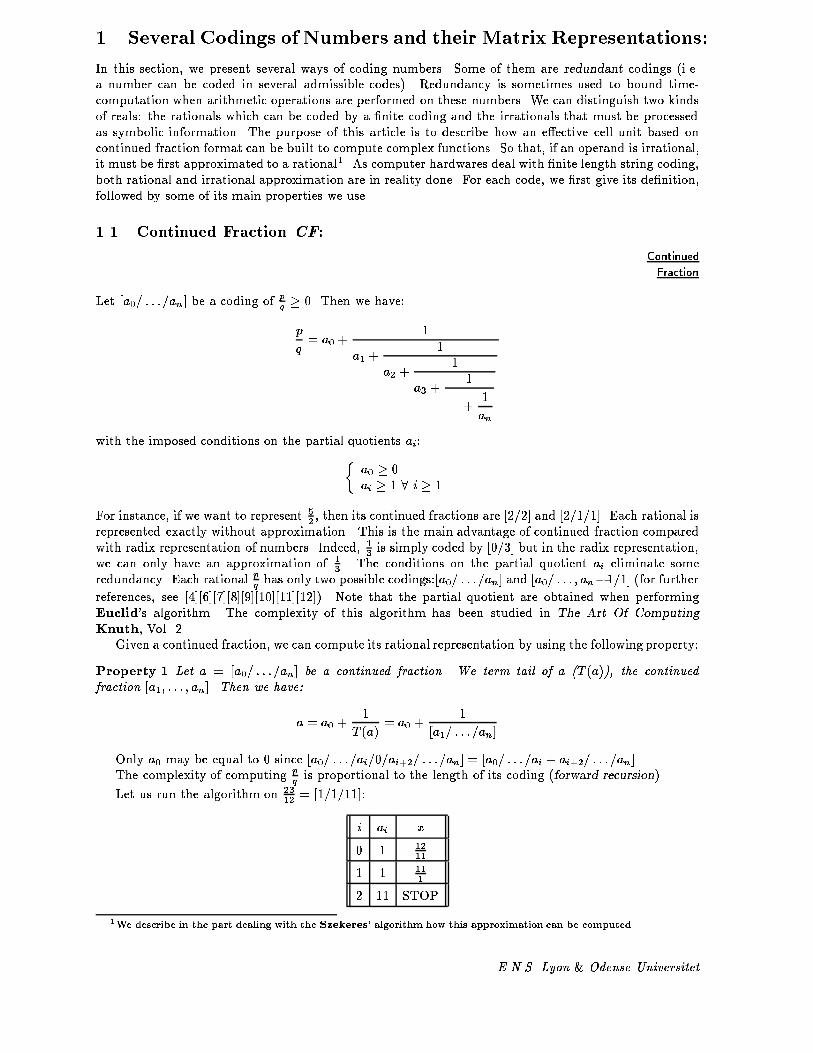
Algorithms on Continued Fractions 31 Several Codings of Numbers and their Matrix Representations:In this section, we present several ways of coding numbers. Some of them are redundant codings (i.e.a number can be coded in several admissible codes). Redundancy is sometimes used to bound time-computation when arithmetic operations are performed on these numbers. We can distinguish two kindsof reals: the rationals which can be coded by a �nite coding and the irrationals that must be processedas symbolic information. The purpose of this article is to describe how an e�ective cell unit based oncontinued fraction format can be built to compute complex functions. So that, if an operand is irrational,it must be �rst approximated to a rational1. As computer hardwares deal with �nite length string coding,both rational and irrational approximation are in reality done. For each code, we �rst give its de�nition,followed by some of its main properties we use.1.1 Continued Fraction CF: ContinuedFractionLet [a0= : : :=an] be a coding of pq � 0. Then we have:pq = a0 + 1a1 + 1a2 + 1a3 + 1... + 1anwith the imposed conditions on the partial quotients ai:� a0 � 0ai � 1 8 i � 1For instance, if we want to represent 52 , then its continued fractions are [2=2] and [2=1=1]. Each rational isrepresented exactly without approximation . This is the main advantage of continued fraction comparedwith radix representation of numbers. Indeed, 13 is simply coded by [0=3] but in the radix representation,we can only have an approximation of 13 . The conditions on the partial quotient ai eliminate someredundancy. Each rational pq has only two possible codings:[a0= : : :=an] and [a0= : : : ; an�1=1] (for furtherreferences, see [4][6][7][8][9][10][11][12]). Note that the partial quotient are obtained when performingEuclid's algorithm. The complexity of this algorithm has been studied in The Art Of ComputingKnuth, Vol. 2.Given a continued fraction, we can compute its rational representation by using the following property:Property 1 Let a = [a0= : : :=an] be a continued fraction. We term tail of a (T (a)), the continuedfraction [a1; : : : ; an]. Then we have:a = a0 + 1T (a) = a0 + 1[a1= : : :=an]Only a0 may be equal to 0 since [a0= : : :=ai=0=ai+2= : : :=an] = [a0= : : :=ai + ai+2= : : :=an].The complexity of computing pq is proportional to the length of its coding (forward recursion).Let us run the algorithm on 2312 = [1=1=11]:i ai x0 1 12111 1 1112 11 STOP1We describe in the part dealing with the Szekeres' algorithm how this approximation can be computed.E.N.S. Lyon & Odense Universitet

Algorithms on Continued Fractions 4ALGORITHM -I { Continued Fraction RepresentationINPUT:x = pq (it is not required that gcd(p; q) = 1)OUTPUT:[a0; : : : ; an] such that pq = [a0; : : : ; an].ALGORITHM:i = 0;repeat ai = bxc;if (x 6= ai) then x := 1x�ai ;i := i+ 1;until (x = ai�1);Given a continued fraction coding [a0= : : :=an], we want to compute its rational value pq ; gcd(p; q) = 1.For that purpose, we use the property 1. This algorithm uses three registers but can only compute thepq (using property 5, we can compute all the convergents with four registers). Since [ai= : : :=an] =ai + 1[ai+1=:::=an ] , if the rational denoted by [ai+1= : : :=an] = p0q0 has been computed, we can compute[ai= : : :=an] = p0�ai+q0p0 = p00q00 .The steps generated by the algorithm when computing the value of [1=1=11] are:i ai p q2 11 11 11 1 12 110 0 23 12If [a0= : : :=an] is a continued fraction representing pq , we term i � th convergent (0 � i � n) thecontinued fraction [a0= : : :=ai] = piqi .Property 2 The sequence (p2iq2i )i of even convergents is increasing and satis�es p2iq2i � pq .Property 3 The sequence (p2i+1q2i+1 )i of odd convergents is decreasing and sati�es p2i+1q2i+1 � pq .Property 4 If [a0= : : :=an] is a continued fraction representing pq with a0 6= 0 then [0=a0= : : :=an] is acontinued fraction denoted qp . It follows, that if a0 = 0 then qp = [a1= : : :=an].n-th convergent Continued Fraction Expansion Rational Decimal Rep.0 [1] 11 11 [1=2] 32 1:52 [1=2=3] 107 1:428571429:::3 [1=2=3=4] 4330 1:433333333:::4 [1=2=3=4=5] 225157 1:433121019:::Convergents of 225157 = [1=2=3=4=5].We de�ne the relational symbol << on the rational as follows: pq<< rs i� p < r and r < s.The convergents are often used when analysing the performance of an algorithmon continued fractions.We cite below the main properties: E.N.S. Lyon & Odense Universitet

Algorithms on Continued Fractions 5ALGORITHM -II { Rational Number RepresentationINPUT:[a0= : : :=an] a coding of a rational number.OUTPUT:pq = [a0; : : : ; an] with gcd(p; q) = 1ALGORITHM:p := an;q := 1;i := n� 1;while(i � 0) do begintmp := q + ai � p;q := p;p := tmp;i := i� 1;endProperty 5 The convergents piqi = [a0= : : :=ai] of any continued fraction pq = [a0= : : :=an] satisfy thefollowing properties:� Recursive ancestry: With p�2 = 0; p�1 = 1; q�2 = 1; q�1 = 0, we have pi = aipi�1 + pi�2 andqi = aiqi�1 + qi�2.� Irreductibility: gcd(pi; qi) = 1.� Adjacency: qipi�1 � piqi�1 = (�1)i.� Simplicity: piqi<< pi+1qi+1 for i � n � 1.� Alternating convergence:p0q0 < p2q2 < : : : < p2iq2i < : : : � pq � : : : < p2i�1q2i�1 < : : : < p1q1� Best rational approximation: rs<< piqi ) jrs � pq j > jpiqi � pq j� Quadratic Convergence: 1qi(qi+1 + qi) < jpiqi � pq j � 1qiqi+1 for i � n� 1� Real approximation: jx � pq j < 12q2 for irreductible pq ) pq is a convergent of a continued fractionexpansion of x.If [a0= : : :=an] is the coding of jpq j, then if pq � 0, its continued fraction is denoted by �[a0= : : :=an] =[�a0= : : :=� an]. E.N.S. Lyon & Odense Universitet

Algorithms on Continued Fractions 61.2 Redundant Continued Fraction: RedundantContinuedFractionRedundancy is often used in arithmetic algorithms([10][16]) where it allows to produce result more quickly(when the result is coded by a continued fraction, redundancy allows to deliver a partial quotient earlier).pq = a0 + 1a1 + 1a2 + 1a3 + 1... + 1anwith the following conditions8<: a0 � 0jaij = 1 ; 1 � i � n� 1 implies that ai and ai+1 have the same signjanj � 2 whenever k � 2The set of all redundant continued fraction expansions of 114 is then114 =8>><>>: [2=1=3][2=2=1=2][2=2=2=2][3=4]The algorithm to determine all the redundant continued fraction representation of pq is more complexsince it uses a recursive process which must take care of the initial 2 steps (a0 and a1). Let us considerthe rational pq . If we choose the partial quotient a, then the remaining rational is qp�aq . Using the factthat j qp�aq j � 1 or jp�aqq j � 1, it follows:a must satisfy the range constraint 8<: a � p+qq = pq + 1a � p�qq = pq � 1a 2 N (1)Then, we iterate the process until the current partial quotient equals pq (in that case pq 2 N).To have all the codes possible given a rational, the conditions on redundancy must be taken intoaccount. If 1 or �1 is chosen, the next partial quotient must have the same sign. If n � 2, we mustensure that the last partial quotient an satis�es an � 2.In order to simplify the algorithm, we use a queue Q in which a value can be added (appended) in itsqueue by the operator �.In the algorithm, we use a boolean function to assert that the partial quotient is in the proper range:for example if COND is the boolean function, COND = COND(:) = COND(a) = (jaj � 2) speci�esthat the partial quotient must have its absolute value greater or equal than 2.Running the algorithm on the rational 114 , we obtain the following step:a0[2; 3] p0q0 Recursive step2 43 a1[1; 2] p00q00 Recursive step1 31 ! a2 = 3! STOP2 �32 a2[�2;�1] p000q000 Recursive step�1 �21 ! a3 = �2! STOP�2 21 ! a3 = 2! STOP3 �41 ! a1 = �4! STOP E.N.S. Lyon & Odense Universitet

Algorithms on Continued Fractions 7ALGORITHM -III { Redundant Continued FractionINPUT:A rational pq ; gcd(p; q) = 1.Initial Call: GiveRedundantCode(p,q,TRUE,Q null).OUTPUT:All the possible redundant codings of pq .ALGORITHM:Procedure GiveRedundantCode(p,q,COND,n,Q);p,q,n: integer;COND: Boolean Function on the next partial quotient a that must be computed ;Q: represents the Queue where the partial quotients are stocked;beginmin := dp�qq e;max := b q+pq c;for i := min to max dobeginif (COND(i)) then dobeginif (n � 1) then NEWCOND:=(a � 2) elseNEWCOND:=a 6= 0;if (jij = 1) then NEWCOND:=NEWCONDV( jaja = i);if (pq = i) then Q Q � i;else GiveRedundantCode(q,p-iq,NEWCOND,n+1,Q� i);endendend

E.N.S. Lyon & Odense Universitet

Algorithms on Continued Fractions 81.3 Continued Logarithmic Fraction: ContinuedLogarithmicFractionThis way of coding rationals allows easy-coding-decoding binary digits. We now consider the followingunique coding of [a0; : : : ; an]CL:pq = 2a0 + 2a02a1 + 2a12a2 + 2a22a3 + 2a3. . . + 2an�12anwith the condition on the logarithmic partial quotients� a0 � 0ai � 1 8 i � 1By factorizing at each level the partial quotient (if we suppose pq � 1, otherwise pq = [0] � [coding of qp ]),we �nd 2a0 + 12a1�a0 + 12a2�a1+a0 + 12a3�a2+a1�a0 + 1... + 12an�an�1+an+2�:::+(�1)na0 =[2a0; 2a1�a0 ; : : : ; 2an�an�1+an+2�:::+(�1)na0 ]which is a continued fraction. We term it continued logarithmic fraction because of the fact that it canbe ciphered just by taking the logarithm in base 2 at each step (the remaining number is qp�2aiq ). Thisfactorization was introduced in an unpublished paper of Gosper in 1977.For instance, if alg.4 is applied to 2811 , we have the following steps:step (i) pq a0i ai sum0 2811 1 = a0 1 11 116 0 = a1 � a0 1 02 65 0 = a2 � a1 + a0 0 03 51 2 = a3 � a2 + a1 � a0 2 24 11 0 = a4 � a3 + a2 � a1 + a0 0 0So �nally, it comes that 2811 = [2=1=1=4=1] = [2=1=1=5] = [1=1=0=2=2]CL.Since the partial quotients of that coding are generally small2, we can code p, a partial quotient, asl(p) = 1p0 (a (p)-string of 1 followed by a 0).Hence, we have l(0) = 0; l(1) = 10; l(2) = 110; ; l(3) = 1110; : : :. With that binary sized coding,CL(2811) = 10 � 10 � 0 � 110 � 110.This simple algorithm can be implemented in hardware with a simple look-up table (this look-up tableis described by a small number of states. For a complete description of that table, see [16]).2From classical material on continued fractions it is known that the partial quotients in the continued fraction expansionof a randomly chosen pq 2 [0;1] ([13]) will have the value i with the probability essentially given by pi = log2 (1 + 1i(i+2) ).E.N.S. Lyon & Odense Universitet

Algorithms on Continued Fractions 9ALGORITHM -IV { Continued Logarithmic FractionINPUT: pq ; gcd(p; q) = 1OUTPUT: [a0= : : :=an]CL = [a00= : : :=a0n]ALGORITHM:i := 0;sum := 0;if (p < q) then begina0 := 0;i := 1;tmp := p;p := q;q := tmp;end;while (q 6= 0) do begina0i := blog2 pq c;ai := a0i + sum;tmp := q;q := p� 2a0iq;p := tmp;sum := a0i;i := i+ 1;end

E.N.S. Lyon & Odense Universitet

Algorithms on Continued Fractions 101.4 LCF - Lexicographic Continued Fraction: LexicographicContinuedFractionThis way of representing rational numbers has been introduced by Matula and Kornerup in 1985([3]).We say a code follows the lexicographic order i� given two strings s(a); s(b) of binary digits denoting therationals a and b: 8<: a < b, s(a) < s(b)a = b, s(a) = s(b)a > b, s(a) > s(b)Note that the relational symbols <;=; > used when comparing a with b, and the relational symbols<;=; > used with s(:) are not the same. If p = 2n +Pn1i=0 bi2i is an integral number, then we de�nel(p) = 1n0bn�1 : : : b0 as its lexicographic coding.For instance, we have l(1) = 0; l(2) = 100; l(3) = 101; l(4) = 11000; : : :.In general case, when we want to code pq , we �rst code the sign, then the partial quotients [a0= : : :=an].Taking into account the fact that the even convergents are smaller than the odd ones, and the sign of therational (Signed LCF), it comes:SLCF ([a0=a1= : : :=an]) = � 1 � LCF ([a0= : : :=an]) for [a0= : : :=an] � 0.0 � LCF (j[a0= : : :=an]j) otherwisewhere, LCF ([a0=a1= : : :=a2n]) = � 1 � l(a0) � l(a1) � : : : � l(a2n) for [a0= : : :=an] � 1.0 � l(a0) � l(a1) � : : : � l(a2n) otherwiseLCF ([a0=a1= : : :=a2n=a2n+1]) = � LCF ([a0=a1= : : :=a2n]) � l(a2n+1) if [a0=a1= : : :=a2n=a2n+1] � 1LCF ([a0=a1= : : :=a2n]) � l(a2n+1) otherwiseWorst case representation-induced precision loss for any real number by a �xed length representablenumber of the system has been shown to be at most 19% of bit word length, with no precision losswhatsoever induced in the representation of any reasonably sized rational number (a complete descriptionof the proof can be found in [3]).Using the probability of ai = j (pj = log2 (1 + 1j(j+2))), it follows that:i pi1 0:4152 0:1703 0:0934 0:059An average partial quotient will be coded, therefore, by n bits wheren =Xi (2blog2 ic + 1) log2 (1 + 1i(i + 2)) ' 3:51:::This yields straigthforwardly the observation([3]):Observation 1 From the known distribution of partial quotient size, it follows that the canonical con-tinued fraction expansion of LCF expansion of a rational pq = [a0= : : :=an] = b0b1b2 : : : bk�11 yields anexpected convergent to convergent ratio of e kn = 3:51:::We conclude the description of LCF by a property on the gap sizes between two adjacents LCFrepresentation coded by a k-string:Property 6 Given � > 0, then for su�ciently large k, the maximum gap size will be at least 2�(a+�)kfor a = 14 log2(5 + 2p6) = 0:82682::: and the minimum gap size will be no bigger than 2(�b��)k forb = log2 3+p52 = 1:38848:::.A description of the proof can be found in [3]. E.N.S. Lyon & Odense Universitet

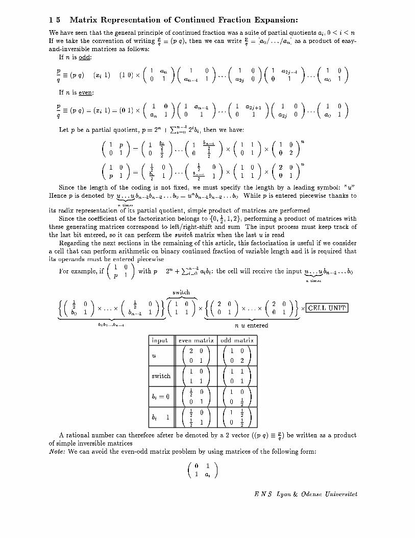
Algorithms on Continued Fractions 111.5 Matrix Representation of Continued Fraction Expansion:We have seen that the general principle of continued fraction was a suite of partial quotients ai; 0 � i � n.If we take the convention of writing pq � (p q), then we can write pq = [a0= : : :=an] as a product of easy-and-inversible matrices as follows:If n is odd:pq � (p q) = (xi 1) = (1 0)�� 1 an0 1 �� 1 0an�1 1 � : : :� 1 0a2j 0 �� 1 a2j�10 1 � : : :� 1 0a0 1 �If n is even:pq � (p q) = (xi 1) = (0 1)� � 1 0an 1 �� 1 an�10 1 � : : :� 1 a2j+10 1 �� 1 0a2j 0 � : : :� 1 0a0 1 �Let p be a partial quotient, p = 2n +Pn�1i=0 2ibi, then we have:� 1 p0 1 � = � 1 b020 12 � : : :� 1 bn�120 12 �� � 1 10 1 ��� 1 00 2 �n� 1 0p 1 � = � 12 0b02 1 � : : :� 12 0bn�12 1 �� � 1 01 1 ��� 2 00 1 �nSince the length of the coding is not �xed, we must specify the length by a leading symbol: "u".Hence p is denoted by u : : :u| {z }n times bn�1bn�2 : : : b0 = unbn�1bn�2 : : : b0. While p is entered piecewise thanks toits radix representation of its partial quotient, simple product of matrices are performed.Since the coe�cient of the factorization belongs to f0; 12 ; 1; 2g, performing a product of matrices withthese generating matrices correspond to left/right-shift and sum. The input process must keep track ofthe last bit entered, so it can perform the switch matrix when the last u is read.Regarding the next sections in the remaining of this article, this factorization is useful if we considera cell that can perform arithmetic on binary continued fraction of variable length and it is required thatits operands must be entered piecewise.For example, if � 1 0p 1 � with p = 2n +Pn�1i=0 aibi: the cell will receive the input u : : :u| {z }n times bn�1 : : : b0�� 12 0b0 1 �� : : :�� 12 0bn�1 1 ��| {z }b0b1:::bn�1 switchz }| {� 1 01 1 ���� 2 00 1 �� : : :� � 2 00 1 ��| {z }n u entered � CELL UNITinput even matrix odd matrixu 2 00 1 ! 1 00 2 !switch 1 01 1 ! 1 10 1 !bi = 0 12 00 1 ! 1 00 12 !bi = 1 12 012 1 ! 1 120 12 !A rational number can therefore afeter be denoted by a 2-vector ((p q) � pq ) be written as a productof simple inversible matrices.Note: We can avoid the even-odd matrix problem by using matrices of the following form:� 0 11 ai � E.N.S. Lyon & Odense Universitet

Algorithms on Continued Fractions 12since � 1 0a2i+1 1 �� � 1 a2i0 1 � = � 1 0a2i+1 1 ��� 0 11 0 �| {z }� 0 11 a2i+1 � �� 1 0a2i 1 ��� 0 11 0 �| {z }� 0 11 a2i �In the last section, we de�ne a multicontinued fraction by means of matrices. The switch matrix isno more used and an homogene writing3 is used.1.6 Radix Coding: RadixWe consider, now as it is often used in pratice, a rational pq in a radix representation (34 = 0:75 =(0:11)2). A number x has its integral part bxc and its fractional part x� bxc. Both parts can be codedin radix representation. A number p = nXi=�k 2ibi = 2nbn+2n1bn�1+ : : :+2�k+1b�k+1+ 2�kb�k is codedas un�1bnbb1 : : : b1b0b�1 : : : b�k with the alphabet B = fu; 0; 1g where u is a leader code allowing to countthe length of the integral part.For instance, 7:375 = (111:011)2 � uu111011.We can also use, more elaborate form of coding based on radix representation ([11][13][16]), like thetwo's complement �xed-point numbers (C-2) ,...1.7 Redundant Binary Representation (RPQ): RedundantRadixIn the algorithm developed later, redundancy will allow us to bound delays between inputs and outputs.Outputs will be produced faster, and the velocity of streams of data in the pipeline computational treewill be higher. LCF provides the bit-grained the structure without redundancy. If p is an integral number,then [p]2 = bn : : : b0 where bi 2 f1; 0; 1g, is one of its coding. We constrain redundancy as follows:R(p) = un�1bnbn�1 : : : b0 with jbnj = 1satisfying the range constraint: 2n�1 + 1 � p � 2n+1 � 1 for n � 2and for p = 0, we have R(p) = b0 = 0.De�nition 1 For n � 2, a self-delimiting signed bit string un�1bnbn�1 : : : b1b0 is admissible i� whenbnbn�1 = 11 or 11, the sign of bn�2bn�3 : : : b1b0 agrees with that of bn.For example, the string (111)2 = 1 is inadmissible but (111)2 = 3 is admissible.The test must be easy to perform, since in practice, a stream of bits will enter piecewise the arithmeticcell.For any redundant continued fraction, we obtain the following coding of pq = [a0= : : :=an]:R(pq ) = R(a0) �R(a1) � : : : �R(an)In general, all the algorithms which deals with the enumeration of redundant representations of anumber are recursive. In the redundant radix representation, the range constraint is de�ned by 2n�1+1 �3The "switch matrix" of a j-multicontinued fraction is unique and de�ned as ej+1 where ej+1 is the (j + 1)-th unitvector in base Qj+1 E.N.S. Lyon & Odense Universitet

Algorithms on Continued Fractions 13ALGORITHM -V { Radix RepresentationINPUT:A real number x.OUTPUT:Its radix representation in the list Q.Note that the operator � is a concatenator. Hence a � b 6= b � a ; a 6= b.Procedure IntegerPart(x,Q);x:integer;Q: queue;beginlength: integer;length := 0;while (x 6= 0) do beginQ (x mod 2) � Q;x := x div 2;length := length + 1;endQ ulength � QendProcedure FractionalPart(x,Q);x:integer;Q: queue;beginif (x=0) then EXIT;if (x � 12) then FractionalPart(2x-1,Q� 1);else FractionalPart(2x,Q� 0);endbeginEmpty(Q);IntegerPart(bxc,Q);Q Q � ":";FractionalPart(x� bxc,Q);end E.N.S. Lyon & Odense Universitet

Algorithms on Continued Fractions 140501001502002500 500 1000 1500 2000Figure 1: Number of redundant codings for integers x 2 [0; 2048].jpj � 2n+1 � 1. Hence, we have blog2(jpj+ 1)c � 1 � n � blog2(jpj � 1)c + 1, which depending on thevalue of jpj gives 2 or 3 di�erent choices for n.Let's take an example: we'd like to have the representations of 10 = (1010)2. Computing the n-rangegives: 2 � n � 4. So, the di�erent kind of format are:8<: b3b2b1b0b4b3b2b1b0b5b4b3b2b1b0Let's take, for instance, the format b4b3b2b1b0. Then, since 10 is positive, we have b4 = 1 but 24 = 16,so we have to code �6 in redundant radix representation with at most format of length 3 : b3b2b1b0 sinceb4 = 1. The last point shows the recursive process.Proceeding in that way, we �nd the 8 di�erent codings for x = 10:The output displayed below is porduced by the MulCF-function program described in annex. Thealphabet denoting the results is f[1]; 0; 1g where [1] denote 1.>1[1][1]1[1]0>1[1][1]010>1[1]0[1][1]0>01[1]1[1]0>01[1]010>010[1][1]0>0011[1]0>001010Note: Redundancy can be present both in the partial quotients (see for example RPQ) and in the binaryrepresentation of these partial quotients.2 Computation of Functions of One Variable:2.1 Notations and Introduction to the Problem:To understand the underlying principles of the general algorithm, we begin by a presentation of thegeneral concept. We want to compute the following function f(x) = ax+cbx+d where x is a variable (x1). TheE.N.S. Lyon & Odense Universitet

Algorithms on Continued Fractions 15ALGORITHM -VI { Redundant Binary RepresentationINPUT:An integer x: call: RedundantNumber(x,"",MAX NUMBER) where MAX NUMBER represents the max-imal number of bits that can be used to code it.OUTPUT:All the redundant binary radix codings for x as de�ned previously.Procedure RedundantNumber(x,s,m)x:integer;m:integer;s: string;beginmincode:integer;maxcode:integer;i:integer;if (x = 0) then Display(s0m); elsebeginmincode := log2 bjxj+ 1c+ 1;maxcode := log2 bjxj � 1c + 3;maxcode := MAX(maxcode;m);for i := maxcode downto mincode dobeginif (x > 0) then RedundantNumber(x� 2i�1,s0maxcode�i1,i-1);else RedundantNumber(x+ 2i�1,s0maxcode�i1,i-1);endendend

E.N.S. Lyon & Odense Universitet

Algorithms on Continued Fractions 161:000000000 11 1=11:500000000 32 1=2=11:570000000 157100 1=1=1=3=14=11:570000000 157100 1=1=1=3=14=11:570700000 1570710000 1=1=1=3=27=1=2=1=1=1=4=11:570790000 157079100000 1=1=1=3=31=1=2=16=4=2=11:570796000 392699250000 1=1=1=3=31=1=41=1=1=2=1=3=11:570796300 1570796310000000 1=1=1=3=31=1=121=3=1=4=3=1=1=2=11:570796320 98174776250000 1=1=1=3=31=1=138=1=2=2=1=4=4=11:570796326 785398163500000000 1=1=1=3=31=1=144=1=18=8=2=1=7=4=1Figure 2: Approximations of �2 .computation can also be seen in term of matrix using the convention x � (p q) if x = pq ; gcd(p; q) = 1 (inpractice, its always the case since irrationals must be approximated to a closer rational according to theselected precision): f(x) � (x 1)�� a bc d � = (p q) �� a bc d �For example, if we take f(x) = 3x+12x+3 , we have the general matrix notation f(x) � (x 1)�� 3 21 3 �.Our algorithm takes its input piecewise and must also deliver output piecewise. Thus, it is possible todevelop a pipeline structure corresponding to the evaluation of a more complex function. If x is coded intoits continued fraction [a0=a1= : : :=an], the partial quotients a0; a1; : : : ; an will be successively entered (thepartial quotient de�nes the size4 of the input). At step i, the �rst i partial quotients will be consumedand the result of f(xi) where xi is the i-th convergent of x is known. It is therefore possible to considera process that approximate a real to a rational written in continued fraction and deliver its successivepartial quotients to the process that compute the function.EVALUATION OF �2 COMPUTATION OF f(�2 )Observation 2 It is worth noting that the (i + 1)-th partial quotient ai(�) determined at step5 � whenperforming approximation of x = [a0=a1= : : : =ai= : : :] is the same as ai i� there exists two consecutivesteps �1 and �2 where ai = ai(�1) = ai(�2).2.2 Consuming Input Piecewise:If we note X = (x 1) = (p q) � x, we can rewrite the function intoY = X �8<: I�1 � I| {z }Identity matrix9=;� F �8<: O�1 �O| {z }Identity matrix9=;We can group the terms in a di�erent wayY = 8><>: X � I�1| {z }input process9>=>; �8><>: I � F � O�1| {z }update process9>=>;�8<: O|{z}output process9=; (2)4The size is seen as a parameter which de�nes the granularity of the atom.5The notion of step, here, denotes the current rational approximation. E.N.S. Lyon & Odense Universitet

Algorithms on Continued Fractions 17ALGORITHM -VII { Consuming InputScan the input until a partial quotient ai+1 is available or the termination signal is perceived. Uponthe termation signal, depending on the parity of i, perform the product of matrices Se � Fi (i is even)or So � Fi (i is odd) else input ai+1 is Fi by multiplyingMi+1 with Fi: Y = X �X(�1)i+1 � (Mi+1 � Fi).where I;O are well chosen inversible matrices (i.e. detO = det I = 1). Given F and the shape of X, itcan be deduced that both I and O are (2� 2) matrices.We can write the latest equation by expanding X � x = [a0= : : :=an] = Mn � : : : � M0 whereMn; : : : ;M0 are inversible matrices representing the partial quotients (we associate the matrixMi to thepartial quotient ai).Property 7 Let x = [a0; : : : ; a2i] be an even continued fraction, then we can rewrite x in term of productsof simple matrices:X = (x 1) = choose rowz }| {(0 1)| {z }Se �� 1 0a2i 1 �� � 1 a2i�10 1 �� : : :�� 1 0a0 1 �if x = [a0; : : : ; a2i+1], then the choose-row matrix is (1 0) ; HenceX = (x 1) = choose rowz }| {(1 0)| {z }So �� 1 a2i+10 1 �� 1 0a2i 1 �� : : :� � 1 0a0 1 �If X is the matrix coding of x = [a0= : : :=a2i], then we can input a suite of Id transformations (thesestransformations can be expressed as M �M�1), namelyY = X��� 1 0�a0 1 ��� 1 a�2i�10 1 �� 1 0�a2i 1 ����� 1 0a2i 1 �� 1 a2i�10 1 �� � 1 0a0 1 ���FExpanding X = M2i � : : :�M0 in the equation and using the fact that M �M�1 = Id, we obtainY = (0 1)� �� 1 0a2i 1 �� 1 a2i�10 1 �� � 1 0a0 1 ��| {z }piecewise input �FLet us denote X2i (X2i+1) the matrix denoting the 2i-th (respectively (2i + 1)-th) convergent of x.Then we can write X �X�12i � (X2i � F )We denote by Fi the result of the product of matrices Xi � F where Xi is the matrix coding the i-thconvergent of x. Since as the end of the algorithm, we will have consumed an (and the current convergentis Xn), we will have X �X�1n � (Xn � F ) = X �X�1N � FnBut as depending on the parity, X = Se �Xn (even parity) or X = Sn �Xn (odd parity), it follows:� n is even: Y = Se � Fn� n is odd: Y = So � FnThe algorithm to consume input is therefore easy. E.N.S. Lyon & Odense Universitet

Algorithms on Continued Fractions 182.3 Producing Output Piecewise:We now focus on the problem of delivering output while inputing. Our result r = f(x) can also be writtenin the continued fraction format. Hence, if r = [b0= : : :=b2j], its matrix representation is (0 1) �M2j �: : :�M0. r = p0q0 � (p0 q0) = � 1 0b2j 1 �� � 1 b2j�10 1 �� : : :� � 1 0b0 1 �We will also denote by Fi the resulting F when (i + 1) inputs have been processed:Fi = � 1 0a2i 1 �� 1 a2i�10 1 ��� 1 0a0 1 �� FAnd for convenience, we will term F the current Fi. So we have always Y = Ci�F at step (i+1) whereCi is the selector matrix de�ned by Ci = � (0 1) () i is even(1 0) () i is oddWhen the i-th input has been consumed, Y � f(xi) where xi is the i-th convergent of x.Y is a two dimensional vector Y = (p0 q0). This vector represents the rational p0q0 which can be writtenin [b0= : : :=b2j]. We must therefore assert that Y denotes always a positive rational number. This de�nesthe output condition.Depending on the parity of the output index, we must check if producing output is possible by assertingthe output condition P(a):P(a) = � F(1) � aF(2) � 0 () output index is even�aF(1) + F(2) � 0 () output index is oddwhere F(i) term the ith column of FIt is worth noting, that if some accumulation of inputs is done, we can just multiply the input matricesand then compute the product of the resulting matrix with the current F . This statement correspondsto the equation Y = X �X�1k � (Mk � : : :�Mi+1)| {z }accumulation �FiY = X �X�1k �M 0 � Fiwhere M 0 represents the product of matrices Mk � : : :�Mi+1:M 0 = Xk �X�1i .We choose, for the velocity of the algorithm, the larger a that satis�es P(a) (in practice, as it ispresented with the generalized matrices, we use the decision hypercube which determines in a constanttime which a, if there exists such a a, must be delivered).When no input can be performed (for instance, 1 has been entered6) then we choose a row of Fdepending on the input parity. This step corresponds to compute the product of matrices Y = Se � Fn(second row) or Y = So � Fn (�rst row). This row represents the rational number p0q0 = r which can berepresented by a continued fraction.We then merge both results (the continued fraction representing p0q0 and the previous results deliveredbefore) taking care of the output parity when the algorithm has read 1 as input. Indeed, if the outputparity is odd, then the next output that could have been produced will be even (and the factorization ofp0q0 begins by a00) so the normalization is already done. Otherwise, we add the �rst coe�cient of p0q0 andthe last output.In term of matrix representation, if [r0= : : :=ri] has been produced like output when the algorithmcatches 1 and if [f1= : : :=fj ] denotes the remaining rational p0q0 , then it follows:Y = X �X�1n � Fj �Mfj � : : :�Mf1 �Mri � : : :�Mr0where Fj = � 1 01 0 � if (j + i � 1) is odd or � 0 10 1 � otherwise.6This can be denoted by a signal in an hardware realization. E.N.S. Lyon & Odense Universitet

Algorithms on Continued Fractions 19ALGORITHM -VIII { FUNCTION OF ONE VARIABLEProcess 1:Consuming inputScan the source until a partial quotient ai (corresponding to the i-th input) is available . Update F byperforming the multiplication of matrices Mi � F .Process 2:Producing outputFind the larger a such that P(a) is satis�ed by intersecting the two interval conditions. Output Mj andupdate F by performing the right-side product of matrix F �M�1j .Process 3:Calling terminationDepending on the output parity, choose the �rst or the second row of the current F .As the �nal result expressed as product of matrices must denote a continued fraction, we must havean alternance of the kind of partial quotient matrices Mfj ; : : : ;Mf0 ;Mri ; : : : ;Mr0 . But as Mf0 is of kind"even", we must have Mri that must be "odd". So that if Mri is not "odd", we insert between Mri andMf0 an Id matrix which corresponds to a null partial quotient.The last case, implies that we must not deliver output directly, but wait that there is another output(partial quotient) to deliver the previous one.In practice, once the termination signal is catched, we input accordingly to the input parity M1 andproduce output until Sinput � F represents a switch matrix (Sinput is the input switch matrix.A graphic simulator MCF-graphic7 that traces each step of the algorithm has been written. Inannex, a LaTEXoutput given by MCF-SIM. is enclosed.Finally, one of the more interesting things, is that we can combine in a same cell both the way weinput and output data. Indeed, in the previous example we have chosen I;O such as they satisfy theinversibility and that our initial vector can also be factorized in the same way as I. Then, without a lotof modi�cation we can use several codes:1. Continued Fraction2. Continued Logarithmic Fraction3. Lexicographic Continued Fraction4. Redundant Partial Quotient (RPQ)5. Redundant Bit-grained Continued Fraction6. Radix7. Redundant radixThe reader is invited to read the �rst section dealing with the codings of numbers ,to see how toproceed. For each format of output, we must change accordingly the output condition. For instance, inthe radix representation, we must perform the sum of the elements belonging to each column of F todetermine how many inputs must be processed before output of the bit of order k can be produced (2k).Indeed, assume we have the bit of 2i as input, then if r denotes the sum of the chosen column, then therelation r2j < 2k must be satis�ed. To bound output delay, we see in that example that it is preferableto have a redundant coding of number which tightens the output delay.7This simulator allows both function of continued fractions and multicontinued fractions to be computedE.N.S. Lyon & Odense Universitet

Algorithms on Continued Fractions 203 Introduction to Generalized Matrices:In this section, we study the computation of a function of n rational variables (X1 = (x1 1); : : : ; Xn =(xn 1)) into the space Q (we denote F this mapping function). F represents a mapping function of Qnto Q expressed as follows: F : Qn! QX1; : : : ; Xn 7�! f(x1; : : : ; xn)We want to provide input piecewise and supply output piecewise, thus allowing a pipelined structure forevaluating complex rational functions.For our purpose, we introduce the notion of generalized matrix in which components are denoted byproduct of matrices which cannot be evaluated while the algorithm runs. Let us consider the followingexample:Consider the matrix M de�ned byM = � a0 b0c0 d0 � = � a1x+ c1 b1x+ d1a2x+ c2 b2x+ d2 �Then M can be rewritten as follows:� a0 b0c0 d0 � = 0BBBB@ (x 1)� � a1 b1c1 d1 �� 10 ! (x 1)�� a1 b1c1 d1 �� 01 !(x 1)� � a2 b2c2 d2 �� 10 ! (x 1)�� a2 b2c2 d2 �� 01 ! 1CCCCAWe can rewrite the previous equation into the following form:� a0 b0c0 d0 � = 0BB@ (x 1)�� a1 b1c1 d1 �(x 1)�� a2 b2c2 d2 � 1CCABy denoting M1 = � a1 b1c1 d1 � and M2 = � a2 b2c2 d2 �, we �nally obtain a compact writing which willbe used in the remaining article: � a0 b0c0 d0 � = (x 1)�M1(x 1)�M2 !The mapping function can, then , be expressed as term of generalized matrix: The computational functionwe allow, can be denoted by:In dimension 2, we allow computation of functions that can be represented by(x1 1)�0BB@ (x2 1)�� a1 b1c1 d1 �(x2 1)�� a2 b2c2 d2 � 1CCAor simpler in (x1 1)� (x2 1)�M (2)1(x2 1)�M (2)2 !And to extend that notion to the general case, we introduce the recursive de�nition of M (�):M (x1) = (x1 1)�� a bc d � and M (x1; : : : ; xn) = (x1 1)� M (x2; : : : ; xn)M (x2; : : : ; xn) !E.N.S. Lyon & Odense Universitet

Algorithms on Continued Fractions 21Each input Xi is characterized by a (1 � 2) matrix (2-vector) representing the variable xi = piqi �(pi qi) = (piqi 1) = (xi 1). We allow transformations on each variable of the following type:T (x) = T (pq ) =ap+bqcp+dq = ax+bcx+d . Since a; b and c; d can also be result of the same kinds of transformations, we can generatewith that recursive process polynomial rational functions of n variables.It is worth noting, that the matrix (xi 1) is multiplied by 2i�1 generalized matrices and that only thematrix variable (xn 1) are multiplied by integral coe�cient 2 � 2 matrix (we term concrete matrix thiskind of matrices, on the contrary we say M is virtual if it iiis a generalized matrix). The computation ofF (x1; : : : ; xn) required then 2n�1 (2� 2){matrix (2n+1 numbers ofZ). The family of functions describedby the recursive process can also be expressed recursively: xiN(xi+1;:::;xn)+N(xi+1 ;:::;xn)xiN(xi+1;:::;xn)+N(xi+1 ;:::;xn) where N is thegeneric recursive functions ; By recurrence hypothesis, it can be shown that the family of functionsgenerated by the process is:F = 8>>><>>>: Xv=(v1;:::;vn)2V B(v) � xv11 : : :xvii : : : xvnNXu=(u1;:::;un)2V B(v) � xu11 : : :xuii : : :xunN 9>>>=>>>;where V is a vector in f0; 1gn and B(o) is the binary number indexed variable representing by o.B((o1; : : : ; on)) = BPni=1 2i�1oiFor instance, taking n = 2, and expanding the sums in the numerator and denominator ,we obtain:F2 = � a � xy + b� x+ c � y + da0 � xy + b0 � x+ c0 � y + d0�Several steps (di�erent kinds of events) are to be observed before describing entirely the algorithm:� The way input data are processed piecewise by allowing interleaved entrance.� The output condition to supply result partial quotient ri� Reducing the depth of the computational tree when a variable has been entirely entered.We also investigate the possibility to change the format of numbers and, hence, combine either rep-resentation of numbers in radix, redundant radix, continued fraction, logarithmic continued fraction,redundant continued fraction, ...In dimension n, the function (f(x1; : : : ; xn)) that can be computed is a fraction of two polynomialfunctions of n variables. f(x1; : : : ; xn) = Pnum(x1; : : : ; xn)Pden(x1; : : : ; xn)De�nition 2 We can write this function in extenso as follows:f(x1; : : : ; xn) = 2n�1Xj=0 q2j n�1Yi=0 x j�2i2ii2n�1Xj=0 q2j+1 n�1Yi=0 x j�2i2iiwhere qj 2 N; 8 j 2 [0; 2n+1� 1] and � represents the binary operator AND(�; �).Developing the kind of function for n = 3 (three variables x1; x2; x3) , we obtain:f(x1; x2; x3) = 7Xj=0 q2j 2Yi=0x j�2i2ii7Xj=0 q2j+1 2Yi=0x j�2i2ii E.N.S. Lyon & Odense Universitet

Algorithms on Continued Fractions 220000 00010010 00110100 01010110 01111000 10011010 10111100 1110 1111 1101Pnum(x1; x2; x3) Pden(x1; x2; x3)x3x2 x1Figure 3: The Gray code on H.We denote by (�)2, the binary representation of a number (for example (1010)2 = 10).f(x1; x2; x3) =q(0000)2+q(0010)2 x1+q(0100)2 x2+q(0110)2 x2x1+q(1000)2 x3+q(1010)2 x3x1+q(1100)2 x3x2+q(1110)2 x1x2x3q(0001)2+q(0011)2 x1+q(0101)2 x2+q(0111)2 x2x1+q(1001)2 x3+q(1011)2 x3x1+q(1101)2 x3x2+q(1111)2 x1x2x3f(x1; x2; x3) = q0 + q2x1 + q4x2 + q6x2x1 + q8x3 + q10x3x1 + q12x3x2 + q14x1x2x3q1 + q3x1 + q5x2 + q7x2x1 + q9x3 + q11x3x1 + q13x3x2 + q15x1x2x3The i-th coe�cient qi can be placed on a 4-hypercube H according to its index i. Numbering thehypercube H with a Gray code, the integral coe�cient qi is positioned on the node that has its Graycode equals to i. The �gure 3 shows how the 4-dimensional hypercube H is numbered with a Gray code.The repartition of the coe�cients qi; i 2 [0; 15] is shown in �gure 4.q15q14 q13q12 q11q10 q9q8 q7q6 q5q4 q3q2 q1q0

Figure 4: Positionning the coe�cients qi on H.E.N.S. Lyon & Odense Universitet

Algorithms on Continued Fractions 233.1 Consuming Input Piecewise:In our algorithm, we can interleave data from any variable once information is available. Hence, a processscans permanently if a partial quotient from any variable is available. Variable (xi 1) denote the rationalpiqi ; gcd(pi; qi) = 1. In the following we develop the update process when variables are entered in termof partial quotients (further types of codings are analyzed at the end of that paper). Let (p q) denotea variable. We have (p q) = (pq 1) = [a0=a1= : : :=an]. Using non-redundant partial quotients, eachvariable (xi 1) can be rewritten in term of products of simple inversible matrix:If n(i) is odd:(xi 1) = (1 0)�� 1 a(i)n0 1 �� 1 0a(i)n�1 1 � : : :� 1 0a(i)2j 0 �� 1 a(i)2j�10 1 � : : :� 1 0a(i)0 1 �If n(i) is even:(xi 1) = (0 1)�� 1 0a(i)n 1 �� 1 a(i)n�10 1 � : : :� 1 a(i)2j+10 1 �� 1 0a(i)2j 0 � : : :� 1 0a(i)0 1 �These matrix factorizations can be expressed simply by two kinds of easy-inversible matrix:� Even Matrix: E(a(i)2j ) = � 1 0a(i)2j 1 �.� Odd Matrix: O(a(i)2j�1) = � 1 a(i)2j�10 1 �.The inverse matrix can also be expressed in term of these generating matrix:� Even Inverse Matrix: E�1(a(i)2j ) = E(�a(i)2j ) = � 1 0�a(i)2j 1 �.� Odd Inverse Matrix: O�1(a(i)2j�1) = O(�a(i)2j�1) = � 1 �a(i)2j�10 1 �.Notice, that the leadingmatrix (0 1) or (1 0) allows to choose among the 2 rows of the (2�2)-matrices :� pi qipi+1 qi+1 � or � pi+1 qi+1pi qi � (this way of proceeding takes into account the reciprocity Euclid'salgorithm).We can rewrite the equation characterizing the computational functional matrix by replacing eachvariable denoted by (xi 1) by its appropriate partial quotient factorization.Then, when an input of any variable is available, say from variable xi, we perform the 2i�1 generalizedproduct of matrix.Indeed, the computational function can be seen as a tree where levels represent the index of variableand left edge, right edge, respectively the M1(:) and M2(:) generalized matrix. Each leaf is a real (2� 2)matrix and each internal node is a virtual matrix. We consider each edge as a link to a (1 � 2) matrix(when all the products after this node as been produced).Suppose that a(i)j is available, updatings on each subtree rooted at a node in depth i � 1 must beperformed in parallel. Depending on the parity on j, we must perform the matrix product O(i) �M orE(i) �M (odd respectively even parity). If M is a real (2 � 2) matrix (i.e. i = n) then that productcan be done directly, otherwise we must update each node in the subrooted tree according the arithmeticoperation.Let us examine, the way we update generalized matrices when we perform a left-side product of amatrix by a generalized matrix:Consider the product � a bc d �� (xi+1 1) �M1(xi+1 1) �M2 !.As we know that M1;M2 are (2 � 2) matrix, we can rewrite the equation such that each of thecoe�cient of the generalized matrix is expressed. E.N.S. Lyon & Odense Universitet

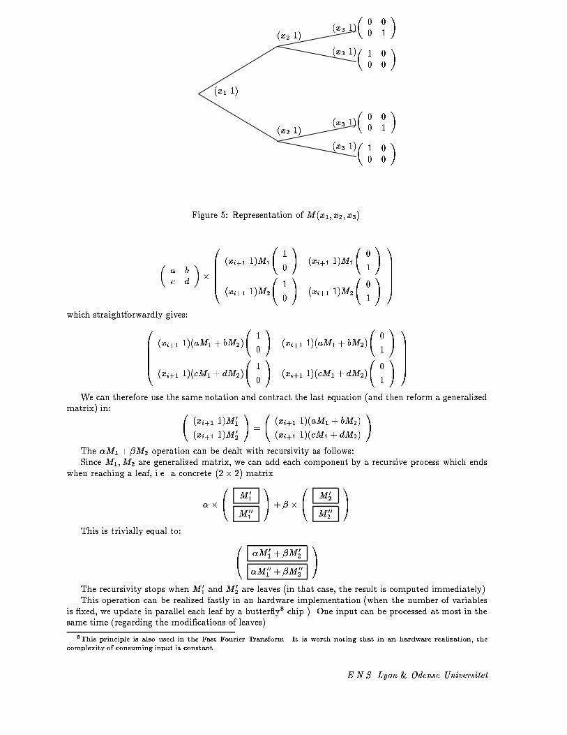
Algorithms on Continued Fractions 24� 1 00 0 �� 0 00 1 �� 1 00 0 �� 0 00 1 �(x3 1)(x3 1)(x3 1)(x3 1)

(x2 1)(x2 1)(x1 1)Figure 5: Representation of M (x1; x2; x3).� a bc d ��0BBBB@ (xi+1 1)M1 10 ! (xi+1 1)M1 01 !(xi+1 1)M2 10 ! (xi+1 1)M2 01 ! 1CCCCAwhich straightforwardly gives:0BBBB@ (xi+1 1)(aM1 + bM2) 10 ! (xi+1 1)(aM1 + bM2) 01 !(xi+1 1)(cM1 + dM2) 10 ! (xi+1 1)(cM1 + dM2) 01 ! 1CCCCAWe can therefore use the same notation and contract the last equation (and then reform a generalizedmatrix) in: (xi+1 1)M 01(xi+1 1)M 02 ! = (xi+1 1)(aM1 + bM2)(xi+1 1)(cM1 + dM2) !The �M1 + �M2 operation can be dealt with recursivity as follows:Since M1;M2 are generalized matrix, we can add each component by a recursive process which endswhen reaching a leaf, i.e. a concrete (2� 2) matrix.��0@ M 01M 001 1A+ � �0@ M 02M 002 1AThis is trivially equal to: 0@ �M 01 + �M 02�M 001 + �M 002 1AThe recursivity stops when M 01 and M 02 are leaves (in that case, the result is computed immediately).This operation can be realized fastly in an hardware implementation (when the number of variablesis �xed, we update in parallel each leaf by a butter y8 chip.). One input can be processed at most in thesame time (regarding the modi�cations of leaves).8This principle is also used in the Fast Fourier Transform. It is worth noting that in an hardware realization, thecomplexity of consuming input is constant E.N.S. Lyon & Odense Universitet

Algorithms on Continued Fractions 253.2 Another Way to Process Input:A partial quotient a must be proceeded according to the i-th variable xi. We can �rst reorganize thecomputational generalized matrix, such as xn is permuted with xi. Then we perform the input byjust performing the 2n�1 multiplications in parallel with � 1 a0 1 � (odd) or � 1 0a 1 � (even). Theproblem is therefore to reorganize the generalized matrix T denoting the function f(x1; : : : ; xi; : : : ; xn)into a generalized matrix T 0 which will denote f 0(x1; : : : ; xn; : : : ; xi) such that f(x1; : : : ; xi; : : : ; xn) =f 0(x1; : : : ; xn; : : : ; xi). This permutation of the variable can be denoted by its unique signature, so thatthe problem is to �nd the transformation which can permute two successive variables xi and xi+1.3.2.1 Analyze in Term of Matrices:Let us consider the factorization T = (xi 1)� (xi+1 1)M1(xi+1 1)M2 !We want to �nd a transformation R, such that if R is applied on T , the new generalized matrixcomputing the same function can be written as:R(T ) = (xi+1 1)� (xi 1)M 01(xi 1)M 02 !Let us develop the function denoted by T according to respectively xi+1 and xi and factorize it againfollowing xi+1 and xi: (xi 1)�0BB@ (xi+1 1)� N1 D1N 01 D01 �(xi+1 1)� N2 D2N 02 D02 � 1CCA(xi 1)� xi+1N1 + N 01 xi+1D1 +D01xi+1N2 + N 02 xi+1D2 +D02 !(xixi+1N1 + xiN 01 + xi+1N2 + N 02 xixi+1D1 +D01 + xi+1D2 +D02)Factorizing: (xi+1 1)� xiN1 + N2 xiD1 +D2xiN 01 + N 02 xiD01 +D02 !(xi+1 1)�0BB@ (xi 1)� N1 D1N2 D2 �(xi 1)� N 01 D01N 02 D02 � 1CCAThe new matrices, corresponding to that computation, areM 01 = � N1 D1N2 D2 � andM 02 = � N 01 D01N 02 D02 �.3.2.2 Using the Hypercube Structure:Processing the input of a partial quotient p of variable xi can be seen as rotating the hypercube suchthat the variable xi takes the orientation of xn and then processing the input of partial quotient p fromvariable x0n = xi. The rotation of the hypercube is always constrained by the orientation of the outputaxis9. Once this rotation is done, processing input can be done by multiplying the (2� 2) input matrixM (p) with the 2n�1 concrete matrices.9The output axis can also be interpreted as variable x0. E.N.S. Lyon & Odense Universitet

Algorithms on Continued Fractions 26Observation 3 Rotating the hypercube H, so that the i-axis and the n� axis are swapped, correspondsfor each node to swap the bit of weight n with the bit of weight i of its Gray code.(xn : : :xi : : : x0)2 ) (xi : : :xn : : :x0)An input of matrice M = � a bc d � in dimension i is noted � a bc d �i. So that if M = � a bc d �is an input corresponding to the i-th variable (xi), we must perform the updating� a bc d �i � Generalized Matrix Denoting f3.3 Shrinking the Computational Tree when an Input is Exhausted:When no more partial quotient can be entered in variable i, i is said to be exhausted (in an hardware, it canbe a speci�c signal or a symbol representing 1 which, in that case, denotes the continued fraction in�niteexpansion. The computational tree can be collapsed into a smaller one where the level corresponding tothe variable i has been deleted and the remaining nodes below level i have been updated according tothe parity of the last input of that variable. The update process is simple since only two cases can occur:� xi ended with odd parity: then the switch matrix is (1 0). And performing the multiplication yieldsto choose the top son.� xi ended with even parity: then the switch matrix is (0 1). And performing the multiplicationyields to choose the bottom son.In term of matrix writing, this correspond to the product:Even Parity: (0 1)� (xi+1 1)M1(xi+1 1)M2 ! = (xi+1 1)M2Odd Parity: (1 0)� (xi+1 1)M1(xi+1 1)M2 ! = (xi+1 1)M1It must be noted,that when an exhaustion operation is performed, the function becomes a function ofn� 1 variables and can then be set to a hypercube of dimension n (instead of n + 1). This correspondsto select the nodes n which gray code satis�es:� xi ends with even parity: n� 2i = 2i� xi ends with odd parity: n� 2i = 03.4 The Output Condition:To allow pipelined evaluation of complex functions, we must also deliver the result piecewise. For thatpurpose, we must assume that the result is in some interval :[r0; r1]Remind that in the case where the output is expressed as a non redundant continued fraction, wehave fpr�1qr�1 ; prqr g if r is oddfprqr ; pr�1qr�1 g if r is evenwhich represent a simplex in dimension 1 (for further information about the simplex, refer to the lin-ear and geometrical book [2]). We must assure that the 4 coe�cients of the matrix (x2 1)M1(x2 1)M2 ! �E.N.S. Lyon & Odense Universitet

Algorithms on Continued Fractions 27� a0 b0c0 d0 � are positive, hence conserving the convex property of the output simplex (the output matrixis � 1 a2r+10 1 � or � 1 0a2r 1 �). Performing the product, we obtain the following generalized matrix:0BBBB@ (x2 1)(a0M1 10 !+ c0M1 01 !) (x2 1)(b0M1 10 !+ d0M1 01 !)(x2 1)(a0M2 10 !+ c0M2 01 !) (x2 1)(b0M2 10 !+ d0M2 01 !) 1CCCCA0BBBB@ (x2 1)M1 a0c0 ! (x2 1)M1 b0d0 !(x2 1)M2 a0c0 ! (x2 1)M2 b0d0 ! 1CCCCAThe operations to determine if an output can be produced are done inside the datastructure since theright-side product of matrix doesn't conserve the datastructure.The frames inside the matrix show the rigidity of the datastructure that must be conserved:0@ M 01 M 001M 02 M 002 1A� � a bc d �We have exibited the two components on our single opaque structure(M1 = M 01 M 001 ) in order toease the visualization. The operations to perform are� M 01 aM 01 + bM 001� M 001 cM 01 + dM 001� M 02 aM 02 + bM 002� M 002 cM 02 + dM 002But since, in the general case, M 01;M 001 ;M 02;M 002 are also generalized matrices, we must execute arecursive process on both the updating and conditions procedures (indeed, we do not know the parityof variables before they end and we must therefore assume the condition on both cases). So, that eachrow of real matrix: e1e2 must satisfy:� ae1 � ce2 � 0� ce1 � ce2 � 0We see that this output condition represents the bottleneck of the algorithm. This output conditioncan nonetheless be computed quickly as described later with the decision hypercube. A more exhaustedstudy and generalization of the output condition is given with the decision hypercube.3.5 Changing the Format of Numbers:In order to have a bitwise grained algorithms, we must re�ne the input and output in the previousalgorithm. This can be achieved by noting the two matrix factorizations of a simple partial quotient.� 1 p0 1 � = � 2n 2n0 1 �� �� 12 bn�10 1 � : : :� 12 b00 1 ��� 1 0p 1 � = � 1 02n 2n ���� 1 0bn�12 12 � : : :� 1 0b02 12 ��E.N.S. Lyon & Odense Universitet

Algorithms on Continued Fractions 28where p = 2n + n�1Xi=0 bi2iWe want to have a one-to-one relation between the bit string in input: un�1bn�1bn�2 : : : b1b0 and thematrix. So that, when one bit is available, the corresponding matrix is applied in our output process.We decompose � 1 02n 2n � into a product of simple matrices:� 1 02n 2n � = � 1 00 2 �n � � 1 01 1 �and � 2n 2n0 1 � in � 2n 2n0 1 � = � 2 00 1 �n � � 1 10 1 �Since our coding is un�1bn�1bn�2 : : : b1b0, we must perform a switch matrix when input switch betweenthe last u and bn�1. This matrix takes into account the u which has been simpli�ed and the matrix� 1 01 1 � or � 1 10 1 �. So that, depending on the parity of the partial quotient, we have:Se = � 1 02 2 �and the odd switch matrix So = � 2 20 1 �These matrices are simple and performing multiplication with another (2�2) matrix just correspondsto shift-or-add operations. In an hardware implementation, each partial quotient must be entered asfollows: a leading sequence of un�1 which indicate the length n, then successively bn�1; : : : ; b0. Forinstance 7 is represented by the binary string 111011. There are many codings that are available (someof them are redundant and allow output to be produced fastly). It is worth noting that we can mixinput/output coding format since each format has its own factorization matrix (see before for a completede�nition of codings).3.6 Computing the Tree-like Matrix Given a Function:We describe in this part an algorithmwhich takes a function f = N(x1 ;:::;xn)D(x1;:::;xn) and give its generalized matrixfactorization following x1; : : : ; xn. We factorize both numerator N (�) and denominatorD(�) following x1.It comes f = x1N1(x2; : : : ; xn) +N2(x2; : : : ; xn)x1D1(x2; : : : ; xn) +D2(x2; : : : ; xn)That function can be written in the matrix form:f = (x1 1)� N1(x2; : : : ; xn) D1(x2; : : : ; xn)N2(x2; : : : ; xn) D2(x2; : : : ; xn) !where N1(�); N2(�); D1(�); D2(�) are obtained by the same process.With the trivial case (which ends the recursivity) f = xia+bxic+d � (xi 1)� � a cb d �.Let us develop the algorithm on f = 3xyz+2xy+3z+y4xyz+2z+3 . The factorization is done successively on x; y; z.Factorization according to x: f = x(3yz + 2y) + (3z + y)x(4yz) + (2z + 3) E.N.S. Lyon & Odense Universitet

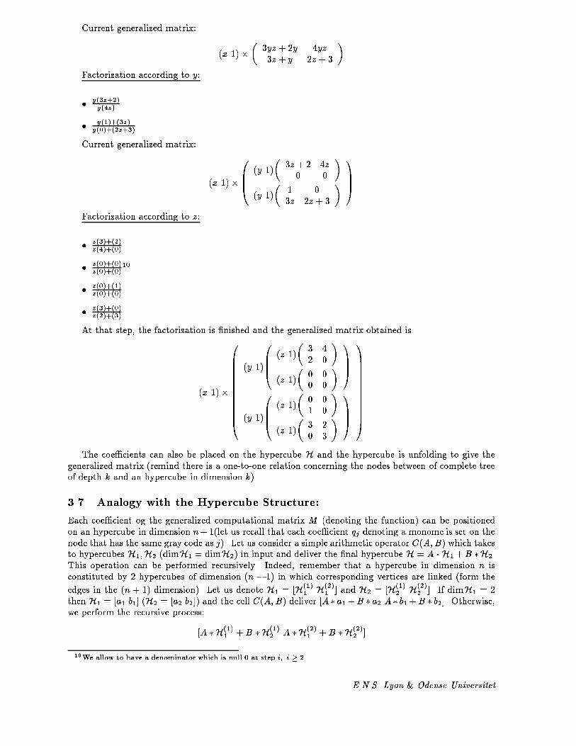
Algorithms on Continued Fractions 29Current generalized matrix: (x 1)�� 3yz + 2y 4yz3z + y 2z + 3 �Factorization according to y:� y(3z+2)y(4z)� y(1)+(3z)y(0)+(2z+3)Current generalized matrix: (x 1)�0BB@ (y 1)� 3z + 2 4z0 0 �(y 1)� 1 03z 2z + 3 � 1CCAFactorization according to z:� z(3)+(2)z(4)+(0)� z(0)+(0)z(0)+(0)10� z(0)+(1)z(0)+(0)� z(3)+(0)z(2)+(3)At that step, the factorization is �nished and the generalized matrix obtained is(x 1)�0BBBBBBBBBBB@ (y 1)0BB@ (z 1)� 3 42 0 �(z 1)� 0 00 0 � 1CCA(y 1)0BB@ (z 1)� 0 01 0 �(z 1)� 3 20 3 � 1CCA 1CCCCCCCCCCCAThe coe�cients can also be placed on the hypercube H and the hypercube is unfolding to give thegeneralized matrix (remind there is a one-to-one relation concerning the nodes between of complete treeof depth k and an hypercube in dimension k).3.7 Analogy with the Hypercube Structure:Each coe�cient og the generalized computational matrix M (denoting the function) can be positionedon an hypercube in dimension n+1(let us recall that each coe�cient qj denoting a monome is set on thenode that has the same gray code as j). Let us consider a simple arithmetic operator C(A;B) which takesto hypercubes H1;H2 (dimH1 = dimH2) in input and deliver the �nal hypercube H = A �H1+B �H2.This operation can be performed recursively. Indeed, remember that a hypercube in dimension n isconstituted by 2 hypercubes of dimension (n � 1) in which corresponding vertices are linked (form theedges in the (n + 1) dimension). Let us denote H1 = [H(1)1 H(2)1 ] and H2 = [H(1)2 H(2)2 ]. If dimH1 = 2then H1 = [a1 b1] (H2 = [a2 b2]) and the cell C(A;B) deliver [A � a1+B � a2 A � b1+B � b2]. Otherwise,we perform the recursive process:[A � H(1)1 +B � H(1)2 A � H(2)1 + B � H(2)2 ]10We allow to have a denominator which is null 0 at step i; i � 2. E.N.S. Lyon & Odense Universitet

Algorithms on Continued Fractions 30� 3 20 3 �� 0 01 0 �� 0 00 0 �� 3 42 0 �(z 1)(z 1)(z 1)(z 1)(y 1)(y 1)(x 1)

Figure 6: Representation of f = 3xyz+2xy+3z+y4xyz+2z+3 .Cell (A;B)a1a2 A � a1 +B � a2a1 b1c1 d1a2 b2c2 d2C(A;B)C(A;B) C(C;D)C(C;D)C(A;B)C(A;B) C(C;D)C(C;D)

Input of (x2 1) A BC D !Hypercubedim. 2.Hypercubedim 3.

Figure 7: Analogy with the hypercube structure.E.N.S. Lyon & Odense Universitet

Algorithms on Continued Fractions 31ALGORITHM -IX { Building the Gray's CodeINPUT:The dimension k of the hypercube to build and the 2k data de�ning the function of k � 1 variables.Call: BuildHyperCube(k,0)OUTPUT:The hypercubeALGORITHM:Function BuildHyperCube(k,x) : HyperCube ;k:integer;x:integer;beginH: HyperCube;if (k = 0) then H = LoadData(x);else H = BuildHyperCube(k � 1; x) BuildHyperCube(k � 1; x+ 2k�1);return H;end;3.7.1 Construction of Gray Code:To develop an e�cient algorithm based on the hypercube structure, we need to enumerate nodes correctlysuch that when an input on xi is done, only particular edges will work. The most famous enumerationof the nodes of an hypercube is Gray code.Property 8 In dimension k, two nodes of the hypercubes are connected by an edge only if their binaryrepresentations di�er with one bit. So that, if n1 = ak�1 : : : a0 and n2 = bk�1 : : : b0 then n1 is connectedto n2 i� XOR(n1; n2) = 2j for some j 0 � j � k � 1. Furthermore, the edge e = (n1; n2) is termed aj-edge connecting the vertices n1 and n2 in dimension j.We denote by � the XOR function. Hence we have XOR(n1; n2) = n1�n2 = n2�n1. The procedureto enumerate the vertices on th k-hypercube (and load data accordingly), is therefore easy:Property 9 If n = bk�1 : : : b0 is a vertex belonging to a k-hypercube, we say n is even (odd) accordingto the i � th dimension i� bi = 1 (respectively bi = 0). So that each j-edge connects an even vertex n1with an odd vertex n2 (furthermore, n1 di�ers from n2 in the (j + 1) bits).3.7.2 Processing Input and Output in the Hypercube H:Inputs are now proceeded e�ciently, considering the parity of its current partial quotient. Let us consideran input of variable xi : Only the (i + 1)-edges will be active. Taking into account the parity of thepartial quotient, the following computations must be performed:� Even Parity: It corresponds to the input matrix � 1 0a 1 � in dimension i. The value of the evenvertex will be changed into ve ve + avo.� Odd Parity: It corresponds to the input matrix � 1 a0 1 � in dimension i. The value of the oddvertex will be changed into vo vo + ave.The output condition is also realized e�ciently according to the �rst dimension (it can be seen as avariable x0). If a can be delivered as output, the remaining coe�cient of each node of the hypercubeE.N.S. Lyon & Odense Universitet

Algorithms on Continued Fractions 32000 001010 011100 101110 111dim 3. dim 1dim 20riginFigure 8: Construction of the Gray Code.must be positive (hence, when the algorithm will be �nished, we select the 1-edge respectively to theparity of variables x1; : : : ; xn.).Illustration of the active edges are shown for a 3-hypercube (function of two variables x1 and x2).3.7.3 The Butter y (./) Operation:We describe in this present part, how to perform a multiplication between a (2 � 2)-matrix M (whichrepresents an input) and an hypercube H in dimension n according to the i-th dimension (variable xi).M can be written as � a bc d �. Then the operation to perform is:� a bc d �i ./ Hwhere ./ denotes the multiplication.If dimH = 2 (one variable x1, H � � q0 q2q1 q3 �) then we de�ne the ./ operation as� a bc d �i ./ H = � a bc d �� � q0 q2q1 q3 �this yields straightforwardly to the matrix� aq0 + bq1 aq2 + bq3cq0 + dq1 cq2 + dq3 �Figure 11 explains why the ./-operation is called "butter y".If dimH = n is greater than 2 then H can be decomposed on to two hypercubes H1 and H2 accordingto the i-th dimension:We eliminate all the i-edges (i.e. the edges that connect two vertices n1 and n2 such that n1�n2 = 2i).We obtain two hypercubes of dimension n � 1. We denote by H1 the hypercube that has all its edgeseven (i-even vertices i.e. if n is a vertex of H1 then n � 2i = 0) and by H2 the one that has all its edgesodd (i-odd vertices i.e. if n is a vertex of H1 then n� 2i = 2i).The butter y operation ./ is de�ned by two steps: the initial step and the recursive step.Homogeneous Step:� a bc d �i ./ H = � a bc d � ./ [H1 i| H2] = [� a bc d �0 ./ H1 i| � a bc d �0 ./ H2]E.N.S. Lyon & Odense Universitet

Algorithms on Continued Fractions 33000 001010100 101110 111a1 b1c1a2 b2c2 d2011d1Figure 9: The 3-hypercube once the coe�cients are loaded.Proceed on Variable Active edges are shown in boldx1x2Output (x0)Figure 10: Active edges according to the i-th axe.E.N.S. Lyon & Odense Universitet

Algorithms on Continued Fractions 34q0 q1q2 q3a bc daq0 + bq1 cq0 + dq1aq2 + bq3 cq2 + dq3Figure 11: The butter y operation (./).Note that the input of the matrix M in dimension i is now 2 inputs of the same matrix M butin dimension 0 (this corresponds to the homogene operation step - it corresponds to a rotation of thehypercube).We must know de�ne how the butter y operation is performed when the matrix must be entered indimension 0. This is de�ned by the unique equationRecursive Step:� a bc d �j ./ H = � a bc d � ./ [H1 i| H2] = [� a bc d �s(j) ./ H1 i| � a bc d �s(j) ./ H2] (3)where s(j) is de�ned according to the �rst step (multiplication in the i-th dimension as follows:s(j) = � j = i � 1! j + 2 jump the initial stepj + 1 otherwise (4)At the last recursive step (this step is de�ned by dimH = 2) j = n (i 6= n) or j = n � 1 (i = n) andwe perform the ./ operation on 2n�1 hypercubes of dimension 2.This observation has leaded to the general property:Property 10 Given a (n + 1) dimensional hypercube H, performing � a bc d �i ./ H corresponds toconsider each i-edge e = (n1; n2) of the hypercube H where n1 (n2) is the value of the even (respectivelyodd) vertex and perform in parallel with the ./ operator.� n1 an1 + bn2� n2 cn1 + dn2Theorem 1 If H is the hypercube coded the generalized functional matrix then entering an input matrixM from variable i corresponds to the butter y operation H Mi ./ H.3.7.4 An example: f(x1; x2; x3) = x1+x2+x3x1x2x3 .To illustrate the previous concept, we develop in this part the steps generated when computing f(x1; x2; x3) =x1+x2+x3x1x2x3 with� x1 = [0=2] = 12� x2 = [0=3] = 13� x3 = [4] = 41 E.N.S. Lyon & Odense Universitet

Algorithms on Continued Fractions 35� 1 00 0 �� 0 01 0 �� 0 01 0 �� 0 10 0 �(z 1)(z 1)(z 1)(z 1)(y 1)(y 1)(x 1)

Figure 12: Generalized matrix of f(x1; x2; x3) = x1+x2+x3x1x2x3 .0000 0001

0100 0101

0110 0111

Z1 Z2

Z3 Z4

Z5 Z6

Z8Z7

00110010

10001001

1011 1010

1101 1100

1111 1110

Z10 Z9

Z11Z12

Z13Z14

Z16 Z15Figure 13: The 4-hypercube used to compute f(:; :; :)The result is f(12 ; 13 ; 4) = 294 � [7=4].The �rst step is to compute the generalized matrix denoting the function (see �gure 12).As the function f(:; :; :) has 3 variables, we must use a 4-hypercube. We represent it as usual whereeach vertex has an integer register which will be updated according the inputs (�gure 13). Each stepof the algorithm is detailed in the �gure 14. According with the parity of each input variable (x1:odd,x2:odd, x3:even), we choose the 0-edge11: 100 � (1000; 1001). The remaining value is 54 which can bewritten as its continued fraction format [1=4]. Hence, our �nal result is [6=0=1=4] = [7=4] (the 0 partialquotient comes from the fact that our output process ends with the even parity). In reality, the algorithmreads the termination signal (1) for x1; x2 and x3. It, then output partial quotients until it can output1. Proceeding in that way, it delivers successively 0=1=4=1.3.7.5 Algorithm on the Hypercube:From the materail developed before, the algorithm on the hypercube structure appears to be quite simple.It �rst loads the generalized matrix on the hypercube and then scans input until no more partial quotientsare to be processed. Each time a partial quotient p is available form xi, it performs the a�p+b-operationon all i-edges. If output can be produced, it delivers the corresponding partial quotient.11We set the bit in the i-th dimension according to the parity of the i-th variable. If xi ends with an odd parity, we set0, otherwise 1. E.N.S. Lyon & Odense Universitet

Algorithms on Continued Fractions 36Events 4-hypercube coe�cientsLoad coe�cients 0000 0001

0100 0101

0110 0111

0 1

0 0

0 0

01

00110010

10001001

1011 1010

1101 1100

1111 1110

0 0

10

10

0 0Input 0 and 2 from x1 0000 0001

0100 0101

0110 0111

0 1

0 0

2 0

01

00110010

10001001

1011 1010

1101 1100

1111 1110

0 2

10

10

0 0Input 0 and 3 from x2 0000 0001

0100 0101

0110 0111

6 1

3 0

2 0

01

00110010

10001001

1011 1010

1101 1100

1111 1110

0 5

10

10

0 0Input 4 from x3 0000 0001

0100 0101

0110 0111

6 1

3 0

2 0

01

00110010

10001001

1011 1010

1101 1100

1111 1110

4 29

130

90

0 4Output 6 0000 0001

0100 0101

0110 0111

0 1

3 0

2 0

01

00110010

10001001

1011 1010

1101 1100

1111 1110

4 5

130

90

0 4Figure 14: Steps generated when computing f(12 ; 13 ; 4)E.N.S. Lyon & Odense Universitet

Algorithms on Continued Fractions 37ALGORITHM -X { Algorithm on the HypercubeINPUT:A generalized matrix representing the function of x1; : : : ; xn.OUTPUT:For a set of value x1 = value1; : : : ; xn = valuen, the result f(value1 ; : : : ; valuen).ALGORITHM:BuildHypercube(n + 1);while(TRUE) dobeginProcess 1: Wait for partial quotient p from xi;Proceed p on each i-th edgeProcess 2: If producing output is possible12, choose the next partial quotient according to the numberrepresentationend;4 An Algorithm Based on the Hypercube to Compute f(x1; : : : ; xn) =Pnum(x1;:::;xn)Pden(x1;:::;xn) :At the end of the previous section, we have introduced the analogy between the generalized matrices andthe hypercubes. Processing input and output on the coe�cient hypercubes have been detailed previously(see the ./ operation) but the e�cient computation of the output condition has been hidden. In thissection, we �rst develop the decision hypercube which allows to compute e�ciently the extremum valuesof the function f and we end with the bit level algorithm which is closed to a concrete implementation13.4.1 The Decision HypercubeIn the algorithm described previously, the bottleneck of the output stream comes from the output condi-tion which required too much time when computed. To eliminate this latency, we introduce the notion ofthe decision14 hypercube, which allows to determinate whether output can be produced or not by com-paring the extremum points of the function. Let us consider the evaluation of a function of n variablesas described before. The main idea is to determine Frange(x1; : : : ; xn) the set of points generated whenx1 2]�1;0; �2;0[; : : : ; xn 2]�n;0; �n;1[. When a partial quotient p of xi has been processed in the coe�cienthypercube, the new variable x0i = 1xi�p has its range in ] 1�i;0�p ; 1�i;0�p [. In particular, whenever the �rstpartial quotient of variable xi has been entered, we know that the tail of xi which corresponds to thenew variable lies between � =]1;1[ and this interval � does not change after, so that �i;0 = 1 and�i;1 =1. The general notation of intervals allows as it will be demonstrated alter to mix various formatsof numbers without changing the theory but only the bounds of variables.Let us consider the non redundant continued fraction when xi 2]1;1[ 8 i 2 [1; n], i.e �i;0 =1 and �i;1 =1 8i 2 [1; n].The Frange point set is de�ned as the result of the function F on the generalized interval I =Qni=1]�i;0; �i;1[ Frange = ff(x1; : : : ; xn) ; 8 x1 2]�1;0; �1;1[; : : : ; xn 2]�n;0; �n;1[gor in the general interval notation13A complete study of the implementation in hardware of the algorithm for two variables x and y has been analyzed in[6]14The decision hypercube contains information about the range where the next partial quotient belonging to the resultlies. This notion was �rst introduce in a paper of Kornerup and Matula in [7]. E.N.S. Lyon & Odense Universitet

Algorithms on Continued Fractions 38Frange = f( nYi=1]�i;0; �i;1[)Hence, if at each step with a little amount of work, Frange is known, we have the information thatthe result is between the bounding limits m and M of Frange where m and M are the extreme valuesof Frange (m = minFrange and M = maxFrange.Observation 4 If [m;M ]\N= frg then we can produce with certitude the output partial quotient r.4.1.1 De�nition of the Decision Hypercube:The function f(x1; : : : ; xn) can be written in f(x1; : : : ; xn) = Pnum(x1;:::;xn)Pden(x1;:::;xn) , where Pnum and Pden areboth polynomial functions of n variables. We build the hypercube as H1H2 where H1 is an hypercubein dimension n in which each vertex de�ned by its binary Gray's code bn : : : b1 contains the value of theevaluation of the function Pnum(T (b1); : : : ; T (bn)) where T (�) is a simple function de�ned as follows:T (biti) = � 1) �i;10) �i;0For example, the vertex v belonging to the hypercube H1 denoted by its Gray's code (01011)2 containsthe value of f(T (1); T (1); T (0); T (1); T (0)) = f(�1;1; �2;1; �2;0; �3;0; �4;1; �5;0). We de�ne in the same waythe n dimensional hypercube H2 denoting the value of Pden.These two hypercubes are linked to form the H-hypercube in dimension n + 1 with a new low bitb0. It is worth noting that since the coe�cients of both polynomes are integers and the bounds of eachvariable are also integers, the nodes of H are integers.We term dn the value stocked in the node having gray code n. It follows thatf(T (b1); : : : ; T (bn)) = Pnum(T (b1); : : : ; T (bn))Pden(T (b1); : : : ; T (bn)) = dbn:::b11dbn:::b10At the beginning of the algorithm , when the coe�cients are loaded on the coe�cient hypercube, wecompute (or load) the value Pnum(T (b1); : : : ; T (bn)) and Pden(T (b1); : : : ; T (bn)) in the decision hypercubefor each b1 2 f0; 1g; : : : ; bn 2 f0; 1g (each vertex of the hypercube H). The extremum values, m and M ,are computed15 (or loaded). We denote by indexm = (mn : : :m1)2 (indexM = (Mn : : :M1)2) the nodewich gray code is indexm (respectively indexM and value d2�indexm+1d2�indexm = m (respectively d2�indexM+1d2�indexM = M ).4.1.2 Updating the Decision Hypercube when an Input is Performed:When processing input of a partial quotient from xi, let say p, we operate the transformation on xi:xi ! xi = p+ 1x0iwhere x0i denote the new variable (x0i 2]1; +1[). Hence, if our function was f(x1; : : : ; xi; : : : ; xn) =xiN+N 0xiD+D0 where N (�); N 0(�); D(�); D0(�) are polynomial functions of n�1 variables x1; : : : ; xi�1; xi+1; : : : ; xn,we have the new function f(x1; : : : ; x0i; : : : ; xn) = xi(N 0 + pN ) +N 0xi(D0 + pD) +DSo that the new coe�cients in the coe�cient hypercube are (updated by the butter y operator) :� N N 0 + pN� N 0 N� D D0 + pD15In reality, these values are only computedwhen the function is well-de�ned. A function is term well-de�ned if it does notadmit a point where the result of the function is unde�ned. This case can occur only when both numerator and denominatorare nulls 00 but 10 is 1 E.N.S. Lyon & Odense Universitet

Algorithms on Continued Fractions 39� D0 Dand the updated value in the decision hypercube are� for the minimum bounding fn(T (b1); : : : ; T (bi�1); T (0); : : : ; T (bn)) = (N 0+pN)�i;0+N(D0+pD)�i;0+D� for the maximum bounding fn(T (b1); : : : ; T (bi�1); T (1); : : : ; T (bn)) = (N 0+pN)�i;1+N(D0+pD)�i;1+DIf we are working with �i;0 = 1; �i;1 =1 8 i 2 [[1; n]] we have� for the minimum bounding fn(T (b1); : : : ; T (bi�1); T (0); : : : ; T (bn)) = (N 0+pN)�i;0+N(D0+pD)+D� for the maximum bounding fn(T (b1); : : : ; T (bi�1); T (1); : : : ; T (bn)) = (N 0+pN)(D0+pD)Re-writing, the last equation in matrix form, we obtain�m bounding! (N 0 + pN )�i;0 + N (D0 + pD)�i;0 +DM bounding! (N 0 + pN )�i;1 + N (D0 + pD)�i;1 +D� = � p�i;0 �i;0 + 1p�i;1 �i;1 + 1 ��� N DN 0 D0 �and with �i;0 = 1; �i;1 =1 8 i 2 [[1; n]]� N 0 + pN + N D0 + pD +DN 0 + pN D0 + pD � = � p+ 1 1p 1 ��� N DN 0 D0 �This generalized operation (dealing with a (2 � 2)-matrix and an hypercube) has been described inthe butter y (./) process. Each time, a new partial quotient is processed, the decision hypercube is alsoupdated accordingly. So that, if the index of m and M can also be updated, the output condition isknown in constant time (O(1)).But let us examine the output process before!4.1.3 Updating the Decision Hypercube when an Output is Performed:If r is the next partial quotient to produce in output, our function can be written as follows:f(x1; : : : ; xn) = r + 1fn(x1; : : : ; xn)When producing output we obtain the new function coded in the coe�cient hypercube fn(x1; : : : ; xn) =1f(x1;:::;xn)�r . If f(x1; : : : ; xn) = x1N+N 0x1D+D0 then the new function isfn(x1; : : : ; xn) = x1D +D0x1(N �Dr) + N 0 �D0rThe analogy with the coe�cient cube can still be done with the right-side product of matrix:� D N �DrD0 N 0 �D0r � = � N DN 0 D0 ��� 1 10 �r �This operation (right-side multiplication) has also been explained in the previous sections (see thebutter y operation ./).4.1.4 Updating the Index of m and M :The purpose of this part is to explain how it is possible to update the index of both extremum valueswith simple process when an input or output is processed. We begin by a nice property linking bothindices (indexm and indexM ). E.N.S. Lyon & Odense Universitet

Algorithms on Continued Fractions 40Property 11 If indexm = (m1 : : :mn)2 is the index of the minimum(whenever the function is wellde�ned) then we have indexM that is de�ned as the complementary binary number:indexM = indexm = (m1 : : :mn)2 = (m1 : : :mn)2It follows from property 11 that only one index has to been known. This property can be proovedusing the well-de�nedness of f and the monotony following variables x1; : : : ; xn.Two cases can occur when the index indexm (and by property 11 also indexM ) must be updated:� Input of partial quotient p from variable xi: The function f can be factorized following xi, whichleads straightforwardly to f(x1; : : : ; xn) = xiN + N 0xiD +D0When we input a partial quotient p from xi we operate the transformationxi ! a+ 1x0iwhere x0i is the new variable lying in the new interval �i =]�i;0; �i;1[ where both �i;0 and �i;1 havebeen updated following the same transformation.This transformation can also be expressed when considering the new variable xi:x0i ! 1xi � pwhich can be decomposed in two steps following the scheme;xi translation�! xi � p inversion�! 1xi � pRegarding the trace of the function in I = Qni=1]�i;0; �i;1[, the transformation acts as follows{ Step 1 : Substract p from xi. This corresponds to translation of the tracing to the "left" (see�gure 15). Since the function is monotonic regarding xi (increasing or decreasing) the indexof both the minimum value and the maximum value have not changed.{ Step 2 : Once step 1 has been processed, we operate the inversion xi ! 1xi . So that if thefunction was increasing regarding xi it becomes decreasing and vice-versa (see bottom of the�gure 15). We have changed both index by ipping the bit mi into mi and Mi into Mi.� Output partial quotient r (from x0): When we output a partial quotient r from the coe�cienthypercube, we perform also accordingly the following diagram:f(x1; : : : ; xn) translation�! f(x1; : : : ; xn) � r inversion�! 1f(x1; : : : ; xn)� rBut if we look at the trace of f each value has been �rst decreased by r so that both the positionwhere min and max are does not change and after we perform the inversion so that the positionwhere min stands, contains now the maximum value and vice-versa(see �gure 16).4.2 The Bit Level Algorithm:We develop here how partial quotient can be entered and output piecewise at the bit level. For thatpurpose, we describe how the algorithm works when partial quotient are entered bitwise. We thenintroduce the general tables for the LCF and RPQ formats. E.N.S. Lyon & Odense Universitet

Algorithms on Continued Fractions 41$m$ �i;1�i;0 m0 M 0 M

x0i = 1xi�pp p+ 1xi �0i;1�0i;0 m0M 0 Translation and Blow UpFigure 15: Transformations of Frange when an input on xi is processed.x0 m Mm Mm0M 0 1m�r 1M�r11

r rx00 = 1x0�rFigure 16: Transformations on Frange when an output is processed.E.N.S. Lyon & Odense Universitet

Algorithms on Continued Fractions 424.2.1 General Principle:Since we can can factorize with products of matrices the partial quotient according to the bit level format,the input process does not change. It is worth noting that the coe�cients of the matrices are simpleand belong to the set S = f�12 ; 0; 12 ; 1; 2g. So that when an input matrix is processed in the coe�cienthypercube, only shift/add/multiplication operations are used. As inputs are processed, Frange the imageset of f is updated. We want also to deliver output piecewise according to a selected format with theeternal condition that the result lies in ]1;1[ (partial quotient interval). Backtracking this condition foreach factorizing matrix M , we obtain the corresponding intervals �M so that if Frange 2 �M then wecan output M (indeed we know that the result lies in ]1;1[).Frange M�! Frange0�i �! �fwhere �i is the initial interval de�ned by Frange and �f is the new interval de�ned when we outputthe matrix M .Denoting by the -sign the output operation, we can write�f = �i Mbut �f is known, so that for each di�erent M , we compute the associated interval�b = �f M�1We describe now the results of the computation for the LCF and RPQ formats. The tables can alsobe found in[16].4.2.2 Using the LCF Format:The lexicographic continued fraction format has been described in the �rst section (pages 1.4{1.4). Wenow give the automate that deliver the sequence of matrices denoting the partial quotient and the di�erentoutput intervals.Given a LCF representation of x = pq ; x 2 Q, the automate (see table 1) delivers the matrix represen-tation of the continued fraction denoted x.In the tables denoting the automate, n stands for the partial quotient an so that in the beginningn is null. The column where stands the matrices describe which transformation must be performed onthe coe�cient hypercube. For example, 35 = [0=1=1=2] has for LCF code the sequence of bits (1010011)2where the �rst bit denote its sign (1:positive) and the second its reciprocity (0 : pq < 1).When using the LCF format as output, at the beginning we set the state of the output to A. If Frangeis in an interval (as de�ned in table 1) then we output the corresponding matrix (or bit) and go to thenew state.Observation 5 If the format we use allow redundancy then there exists at least one state S where someof its intervals overlap4.2.3 Using the RPQ Format:We give here in table 2 the automate characterizing the RPQ format. Please note that m denotes the 1bit.For example, we can see that the RPQ format is redundant if we take the inserection of intervals:� State A: ]� 2; 2[\]� 4; 0[6= ;� State B: ]� 1;1[\]� 2; 2[6= ; E.N.S. Lyon & Odense Universitet

Algorithms on Continued Fractions 43State Interval Bit Digit Matrix New n New Statestart � � � 1 00 1 � 0 AA [0;1[ 1 � 1 00 1 � 0 B(sign) ]�1; 0[ 0 � �1 00 1 � 0 BB [1;1[ 1 � 1 00 1 � 0 C(reciproc:) [0; 1[ 0 � 0 11 0 � 0 EC [2;1[ 1 � 2 00 1 � n+ 1 C(Unary mode normal) [1; 2[ 0 � 0 11 �1 � n Dn6=0; En=0D [2;1[ 0 � 12 00 1 � n� 1 Dn6=0; En=0(Binary mode normal) [1; 2[ 1 � 12 0�12 1 � n� 1 Dn6=0; En=0E [2;1[ 0 � 2 00 1 � n+ 1 E(Unary mode reverse) [1; 2[ 1 � 0 11 �1 � n Fn6=0; Cn=0F [2;1[ 1 � 12 00 1 � n� 1 Fn6=0; Cn=0(Binary mode reverse) [1; 2[ 0 � 12 0�12 1 � n� 1 Fn6=0; Cn=0Table 1: The automate characterizing the LCF code.State Interval Bit Digit Matrix New n New Statestart � � � 1 00 1 � 0 AA ]� 1; 1[ 0 � 0 11 0 � 0 A(Unary) ]0; 4[ 1 � 0 21 �2 � n+ 1 B]� 4; 0[ m � 0 21 2 � n+ 1 B]� 2; 2[ u � 1 00 3 � n+ 1 AB ]1;1[ 1 � 12 0�12 1 � n� 1 Bn6=0; An=0(Binary) ]�1;�1[ m � 12 012 1 � n� 1 Bn6=0; An=0]� 2; 2[ 0 � 12 00 1 � n� 1 Bn6=0; An=0Table 2: The automate characterizing the RPQ code.E.N.S. Lyon & Odense Universitet

Algorithms on Continued Fractions 445 The Szekeres Multidimensional Continued Fraction:In this present section, we formalize the algorithm described by Szekeres in term of products of simpleinversible matrix. We then apply these transformations in the computation of complex functions. G.Szekeres introduced new algorithms for generating higher dimensional analogue of the ordinary continuedfraction expansion of a single real number. The algorithmdescribed in the remaining, takes a real k-vector(�1; �2; : : : ; �k) and deliver a (k+1)-vector in Nk+1 : (a1; a2; : : : ; ak; b) where a1b ! �1; a2b ! �2; anb ! �n(if8 i 2 [[1; k]]; �i 2 Q then the algorithm ends with �i = fracaib). Szekeres conjectured, on the basisof extensive computation, that the intermediate vectors produced by the algorithm contains the bestsimultaneous rational approximations to (�1; : : : ; �k).5.1 Best and Good Rational Approximation to a real:As the continued fraction contained in ]0; 1] are the reciprocal of those contained in [1;1[, we supposethat 0 < �i < 1 8 i 2 [[1; k]]. It is known from the Theory of Numbers that each number can be writtenin a continued fraction (which is in�nite when it is an irrational).� = [a1=a2=a3=:::] ; ai > 0 (5)We say PQ is a best rational approximation to � when jQ�� P j < jq� � pj for all rationals pq with0 < q < Q. The sequence of convergents pnqn = [a1= : : : ; an] is then precisely the sequence of bestapproximations to �.We term good rational approximation to � when jQ��P j< 1Q j. In that case, the sequence rpn+1+pnrqn+1+qnwith 1 � r < an+2;n 2 f0; 1; 2; :::g of intermediate convergents contains the sequence of good approxi-mations to �.5.2 Good and Best Rational Approximations of a real k-vector:We can extend the previous notion to higher dimension. Given a � k-vector: � = (�1; : : : ; �k), we wantsimultaneous rational approximations P1Q ; : : : ; PkQ to �1; :::; �k with the same common denominator Q.We say (P1; P2; : : : ; Pk; Q) is a best approximation ifmax1�i�kfjQ�i � Pijg < max1�i�k fjq�i � pijg (6)for all the rational k-tuples p1q ; : : : ; pkq with 0 < q < Q.We say that (P1; P2; : : : ; Pk; Q) is a good approximation ifmax1�i�kfQ 1k jQ�� Pijg < 1 (7)In the following section, we describe an algorithm that takes a real vector and gives its best rationalapproximation where the denominator of each rational is the same.5.3 Algorithm to Compute Approximations to a Real k-vector:We �rst suppose without loss of generality that the real vector � = (�1; : : : ; �k) to approximate isconstrained by 1 > �1 > �2 > : : : > �k > 0 (8)Indeed, we can memorize the sign of �i �rst, so that we input only non negative real numbers. Ifone component is null, then the problem is to approximate a (k � 1) real vector. We can also beforeprocessing normalize the real vector by n = 1maxifaig+1 so that the resulting vector �0 = (�1n ; : : : ; �kn )satisfy the input condition.We must also assume that 1; �1; �2; : : : ; �k are linearly independent over the rationals, i.e.:a0 + kXi=1 ai�i = 0) nXi=0 jaij = 0 (9)E.N.S. Lyon & Odense Universitet

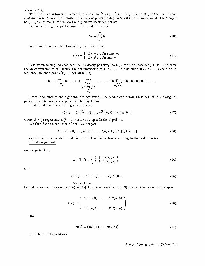
Algorithms on Continued Fractions 45where ai 2 Q.The continued k-fraction, which is denoted by [b1=b2= : : :] is a sequence (�nite, if the real vectorcontains no irrational and in�nite otherwise) of positive integers bi with which we associate the k-tuple(�1; : : : ; �k) of real numbers via the algorithm described below:Let us de�ne sm the partial sum of the �rst m results:sm = mXi=1 bi (10)We de�ne a boolean function �(n) ; n � 1 as follow:�(n) = � if n = sm for some mif n 6= sm for any m (11)It is worth noting, as each term bi is strictly positive, (sm)n2Nform an increasing suite. And thenthe determination of �(:) insure the determination of b1; b2; : : :. In particular, if b1; b2; : : : ; br is a �nitesequence, we then have �(n) = 0 for all n > sr .000 : : :0 1n1|{z}n1=b1 000 : : :000 1n2|{z}n2= b1|{z}n1 +b2 : : : : : : : : :00 1nr|{z}nr=sr 000000000000! : : : : : :Proofs and hints of the algorithm are not given. The reader can obtain these results in the originalpaper of G. Szekeres or a paper written by Cusic.First, we de�ne a set of integral vectors A:A(n; j) = (A(1)(n; j); : : : ; A(k)(n; j)) ; 8 j 2 [[0; k]] (12)where A(n; j) represents a (k + 1) vector at step n in the algorithm.We then de�ne a sequence of positive integer:B = (B(n; 0); : : : ; B(n; i); : : : ; B(n; k)) ; n 2 f0; 1; 2; : : :g (13)Our algorithm consists in updating both A and B vectors according to the real � vector.Initial assignment:we assign initially: A(i)(0; j) = � 0; 0 � j < i � k1; 0 � i � j � k (14)and B(0; j) = A(0)(0; j) = 1; 8 j 2 [0; k] (15)Matrix FormIn matrix notation, we de�ne A(n) as (k + 1) � (k + 1) matrix and B(n) as a (k + 1)-vector at step n.A(n) = 0B@ A(0)(n; 0) : : : A(0)(n; k)... . . . ...A(k)(n; 0) : : : A(k)(n; k) 1CA (16)and B(n) = (B(n; 0); : : : ; B(n; k)) (17)with the initial conditions E.N.S. Lyon & Odense Universitet

Algorithms on Continued Fractions 46A(0) = 0BBBB@ 1 : : : : : : 10 .. . 1... . . . . . . ...0 : : : 0 1 1CCCCA (18)A(0)�1 is therefore: A(0)�1 = 0BBBBB@ 1 �1 0 : : : 00 1 �1 : : : 0... . . . �1 ...0 : : : 0 1 �10 0 : : : : : : 1 1CCCCCA (19)B(0) = (1 1 : : : 1) (20)The new state described by B(n+1) and A(n+1) is achieved by performing a transformation denotedby T (�(n+1); �(n)) where �(n) is an integer bounded by 0 � �(n) � k determined in step n by a procedurewhich is detailed later. Note that this way of proceeding is inductive.Transformation on A:A(i)(n + 1; 0) = (1� �(n + 1))A(i)(n; 0) + �(n+ 1)A(i)(n; �(n)) ; i 2 [[0; k]] (21)A(i)(n+ 1; �(n)) = A(i)(n; 0) + A(i)(n; �(n)) ; i 2 [[0; k]] (22)A(i)(n+ 1; j) = A(i)(n; j) ; 1 � j � k; j 6= �(n) (23)Matrix FormThe transformation associated is denoted by T (�(n+1); �(n)) where �(n+1) is a boolean value and �(n)locates the transformation.By denoting I the identity matrix and ei, the (k + 1) vector, where only i-th component as value 1and the others 0, it follows:T (�(n+ 1); �(n)) = T (�; �) = I + �(e� � e0)eT0 + e0eT� (24)T (�; �) = 0BBBBBBBB@ 1� � 0 : : : 1 : : : 00 1 : : : 0 : : : 0... ... . . . ... ...� 0 : : : 1 : : : 0... ... ... . . . ...0 0 : : : 0 : : : 1 1CCCCCCCCAComputations generated by these transformations are very simple since � is a boolean value.� � = 0 T (0; �) = 0BBBBBBBB@ 1 0 : : : 1 : : : 00 1 : : : 0 : : : 0... ... . . . ... ...0 0 : : : 1 : : : 0... ... ... . . . ...0 0 : : : 0 : : : 1 1CCCCCCCCAE.N.S. Lyon & Odense Universitet

Algorithms on Continued Fractions 47� � = 1 T (1; �) = 0BBBBBBBB@ 0 0 : : : 1 : : : 00 1 : : : 0 : : : 0... ... . . . ... ...1 0 : : : 1 : : : 0... ... ... . . . ...0 0 : : : 0 : : : 1 1CCCCCCCCAThe rank of these transformations are rank(T (�; �)) = k + 1.Transformation on B: B(0; j) = A(0)(n+ 1; j) (25)B(n) is always the �rst row of A(n)We call the a(n) k-vector the n-th approximation fraction to � de�ned bya(n) = (A(1)(n; �(n� 1))B(n; �(n� 1)) ; : : : ; A(k)(n; �(n� 1))B(n; �(n� 1)) ) (26)which is written by factorizing out the common denominator,a(n) = 1B(n; �(n� 1)) (A(1)(n; �(n� 1)); : : : ; A(k)(n; �(n� 1))) (27)To complete our algorithm, we must specify the computation of �(n) and �(n+ 1). For that purpose,we de�ne the set of (k + 1) positive real numbers �(n) = f nj : 0 � j � kg ; n 2 f0; 1; 2; : : :g where�(0) = 8<: 00 = 1� �1 0j = �j � �j+1 ; j 2 [[1; k� 1]] 0k = �k (28)Note that since we have ensured 1 > �1 > : : : > �j > �j+1 > : : : > �0 > 0, 0j > 0 ; 8 j 2 [[0; k]].Then, �(n+ 1) is determined as follow:�(n + 1) = � 0 if n0 > n�(n)1 if n0 < n�(n) (29)We express now the inductive process which de�ne the transition from �(n) to �(n+ 1): (n+1)0 = (1 � 2�(n+ 1))( n0 � n�(n)) (30) (n+1)�(n) = �(n+ 1) n0 + (1� �(n + 1)) n�(n)) (31) (n+1)j = nj ; for 1 � j � k; j 6= �(n) (32)Matrix FormLet us consider �(n) as a (k + 1)-vector, namely:�(n) = 0B@ n0... nk 1CAThe following transformation depending on � must be performed in order to obtain �(n+ 1):E.N.S. Lyon & Odense Universitet

Algorithms on Continued Fractions 48T�(�) = 0BBBBBBBB@ �#1� 2� 0 : : : 2�� 1 : : : 00 1 0 : : : 0... . . . ... ... ...�! � : : : 0 1� � : : : 0... 0 . . . ...0 : : : : : : : : : 0 11CCCCCCCCA (33)�(1) can be rewritten as I� � �T where I� is a (k + 1)� (k + 1) matrix de�ned byI� = 0BBBBBBBBB@ 1 �1 0 : : : : : : 00 1 �1 (0) ...... . . . . . . ...... (0) . . . . . . ...0 : : : : : : 0 1 �10 : : : : : : : : : 0 1 1CCCCCCCCCA (34)In order to complete the description of the algorithm, we must now describe the computation of �(n).But before, we recall the reader on the � relation between two vectors. Given a; b two vectors (which weorder increasingly by a permutation of their components, in a0; b0) , we say a � b if there exists an indexj such as a0j < b0j and 8i 2 [1; j � 1] ; a0i = b0j .We de�ne the (k + 1)-vector V (n; j) = A(n; j)B(n; j) � A(n; 0)B(n; 0) (35)Then �(n) (recall that 1 � �(n) � k) is de�ned to be the largest integer t such that for everyi ; 1 � i � t, we have V (n; i) � V (n; t) or V (n; j) = V (n; h) (36)It follows straightforwardly from the de�nition of �(:) that �(0) = k.It must be noted that if � is a rational vector (embedded in R space), then the algorithm will stop atsome step n. Indeed, we have therefore�(n) = 0BBB@ 00...0 1CCCA = (0) (37)8 t > n; �(t) = 0 (38)In the general case, where at least one of the components �i is irrational, Szekeres has proved thatlimn!1 nj = 0 ; 8 j 2 [[0; k]] (39)5.4 Application of the Szekeres' Algorithm in the Computation of Y = F�X:We want to compute Y = X � F where X is a (k + 1)-vector de�ned by (d a1 : : : ak) representing thepoint (a1d : : : akd ) of Qk which is computed by the Szekere's algorithm with rationals �1; : : : ; �n thatare known piecewise and F is a (k+1�2) matrix (the result is an ordinary continued fraction). We wantto process inputs and deliver output piecewise. Inputs are entered in continued fraction format and canE.N.S. Lyon & Odense Universitet

Algorithms on Continued Fractions 49ALGORITHM -XI { Szekeres' algorithmInput:A vector � = (�1; : : : ; �k) which satis�es 1 > alpha1 > : : : > �i > �i+1 > : : : > alphak > 0 (see 8).Output:A k-multicontinued fraction, best approximation of �. If � has one of its component irrational, thenthe user must choose a step n where he wants to have his approximation (he breaks the loop), else thealgorithm stops at a step denoted also by n. The approximation to � can be obtained from the remainingA (see equation 8).Algorithm:� = k;� = I� � �T ;� =ComputeEpsilon(�);A = A(0);while(NotFinished(�)) dobeginA = A� T (�; �);� =ComputeMu(A);� =ComputeEpsilon(�;�);� = T�(�) � �;end;

E.N.S. Lyon & Odense Universitet

Algorithms on Continued Fractions 500 11 3211 107Figure 17: Convergence of a ai(r) to ai for [1=2=3] = 107 .be interleaved (for instance, we process the partial quotient p(i)j of variable aj, then partial quotient p(l)kof variable al). If one of the input variables is an in�nite continued fraction, then, our algorithm has anin�nite number of steps, but the result is re�ned at each step such that we can have an approximationto the exact result at any step. Referring to the Szekeres' algorithm, we can factorize the n-th rationalapproximation to Xt inXT (n) = A(0)� fT (�(1); �(0)) : : :T (�(i); �(i� 1)) : : :T (�(n); �(n� 1))g| {z }A(n) �eT�(n�1) (40)where eT�(n�1) is the transposed (�(n� 1) + 1)-th unit vector which choose the right column in A(n).eT�(n�1) = 0BBBBBBB@ 0...�(n� 1) line! 10...01CCCCCCCA (41)We can output piecewise by the same process described in the computation of Y = F �X. The mainproblem is to provide input piecewise, i.e. to deliver transformation T (�(i); �(i)). This problem is thesame as to compute �(i) when the current inputs ,that have already been processed , approximate X.We must assume for correctness of calculus, that the transformation T (�(i); �(i)) done when a certainamount of input data have been entered, is the same as if we have waited for all inputs to be entered andthen produce the transformations.As input data are entered in continued fraction format, we can know if the current variable ai(r)(ai(r) =[a(i)0 = : : :=a(i)r ] is the r-th convergent approximated to ai) is lower or greater than ai. Indeed, it dependsonly on the parity of r. If r is even then ai(r) � ai else ai(r) � ai.Considering the �rst step of the algorithm, i.e. case n = 0, we must determine when �(1) can beknown surely. For that purpose we must determine if�(1)� 0 if 00 > 0k:1 if 00 < 0k: (42)But 00 = 1� �1 and 0k = �k, so we must determine which case is true:�(1)� 0 if 1� �1 > �k:1 if 1� �1 < �k: (43)Using the property of increasingness of the even convergents a0; a2; : : : ; a2i; : : : and decreasingness ofthe odd convergents a1; a3; : : : ; a2i+1; : : : (see �gure 17), it comes that 1� (�1 + �k) > 0 is true when itcan be determined safety that (�1+�k) is a upper bound (parity of both �1 and �k is odd) . Proceedingin the same way, we can assert that 1� (�1 + �k) < 0 is true when �1 and �k are even and their sum isgreater than 1. To resume, computation of �(1) can be achieved when �1 and �k have the same parityand their sum assert the condition (in their current approximation to the initial value).�1�k odd evenodd Determined if 1 > �1 + �2 Waiteven Wait Determined if �1 + �2 > 1E.N.S. Lyon & Odense Universitet

Algorithms on Continued Fractions 51The general problem is to give the boolean value of 0 > � at a step of the algorithm where onlysome, but not all, the inputs have been processed.Let us call � the state of the algorithm described by the inputs already entered:� = (�01; : : : ; �0k) (44)where �0i is the last approximation to �i done by considering the input a(i)0 ; : : : ; a(i)r(i) (r(i) + 1 partialquotient of �i have been processed so far).�0i = [a(i)0 ; : : : ; a(i)r(i)]We will design by ni(�) the approximation of ni at step n when � is the current state. The problemis to deliver the state of " n0(�) > n�(�)" which can take three di�erent values:� TRUE in that case, we have ni > n0 when � is known.� FALSE: in that case, we have ni < n0 when � is known (remind that ni 6= n0).� UNDETERMINED: When either TRUE or FALSE can be decided.Our algorithm gives bound to the value ni: ni(�) ��ni(�) � ni � ni(�) + �ni(�) (45)The value of " n0(�) > n�(�)" can be determined only if:� n0(�) ��n0(�) > n�(�) + �n�(�), and in that case, the result is TRUE.� n0(�) + �n0(�) < n�(�) ��n�(�), and the result is FALSE.Otherwise, the result is UNDETERMINED and we must wait for another input aj(i) which willchange � in �0.We ensure that each trust interval associated with ni is non-increasing when � changes to �0.Once �(n) can be computed, we must update � and �:� �(n) = 1 n0 = (n�1)�(n�1)� (n�1)0 (46) n� = (n�1)0 (47)� �(n) = 1 n0 = (n�1)0 � (n�1)�(n�1) (48) n� = (n�1)�(n�1) (49)The decide to stock ni as a function linear function of �i with integral coe�cient, hence performing"symbolic" calculus upon these functions. ni(�) = kXj=0 aij(n)�j (50)where, for convenience of writing, we have �0 = 1.When a transformation cannot be decided because of its UNDETERMINED state, more inputsmust be performed (leading to a �0 state), shrinking the value of �i ; i 2 [1; k], and then shrinking theinterval �(�) into �(�0).At each time a computation of �(n) is possible or an input is proceeded, we �rst compute the newtrust interval and then check is we can perform a new transformation.E.N.S. Lyon & Odense Universitet

Algorithms on Continued Fractions 52��n�2�1�0 ��� �1�2�3�n�n�3

�2�1Function (�)

�1 �n1

0 1 2 n Figure 18: Computing Transformations PiecewiseThe trust intervals are computed as follows:�ni(�) = kXj=0 aij(n) ���k(�) (51)where ��0 = 0 and ��i �!�0= j�i(�) � �i(�0)j.Then, the boolean value of n0 > n� can already be known, if in state �, we have: 0(�)��0(�) > �(�) + ��(�)or 0(�) + �0(�) < �(�)���(�)Otherwise, more inputs have to be processed, and updatings on � and � are done, until one of thetwo conditions is satis�ed.6 An Algorithm for Computing Functions On Variables Enteredin Multicontinued Fractions Format:In this section, we show brie y how an algorithm based on multicontinued fractions can be developedusing the same principles described in the previous sections. We �rst de�ne a k-multicontinued fraction(by means of an algorithm) and associates its matrix representation. Then we show how it is possibleE.N.S. Lyon & Odense Universitet

Algorithms on Continued Fractions 53ALGORITHM -XII { Computing a k-Multicontinued FractionINPUT: A (k + 1)-vector of Nk+1: x = (p1 : : : pk q) with q > 0.OUTPUT: The k-multicontinued fraction [f0; s0; : : : ; fn; sn] denoting x.ALGORITHM:i := 0;while (x 6= ek+1) dobeginFor each i 2 [[1; k]] do p0i := bpiq c;fi = (p01 : : : p0k)x := (p1 � p01q : : : : : : pk � p0kq q);Choose j such as pj = maxi2[[1;k]]fp1; : : : ; pkg;q0 := b qpj c;si := q0 � ej ;i := i + 1;endto follow the path of the previous algorithm and extend the computational function to several variablescoded by multicontinued fractions.6.1 De�nition of a k-multicontinued Fraction:We represents by x = (p1 : : : pk q) the point of Qk de�ned by the k-uplet (p1q : : : pkq ). Given a pointP of Rk, we can �rst approximate by the Szekeres' algorithm P to P 0 such as P 0 is now a point of Qk.P 0 can be represented by a (k+1)-vector x = (p1 : : : pk q). We associate to x a multicontinued fractionde�ned by x = [f0; s0= : : :=fn; sn]where fi; si 8 i 2 [[0; n]] are k-vectors of Nk de�ned successively by the following algorithm:Given a (k + 1)-vector x = (p1 : : : pk q) with q > 0 of Qk+1 denoting a point of Qk, we compute itsmulticontinued fraction by applying to x a succession of two steps.x = (p1 : : : pk q) = (p1 : : : pk)qComputing fi; si:� Step 1: Processing the numerator pi 8 i 2 [[1; k]] Compute for each numerator pi the integer numberai such as pi � aiq � 0. For each i do x := x� aiqei.� Step 2: Processing the denominator q Find pj such as pj is the maximum value and compute bde�ned by q � bpj � 1. Compute x := x� bpjek+1.We obtain a new (k + 1)-vector x0. If x0 = ek+1 then we stop the algorithm (this corresponds to the1 signal) else we inject x0 and obtain fi+1; si+1,...For example, if we run the algorithm on the 3-vector of N3 (5 3 7) denoting a point of Q2 then we �nd:1. � f0 = (0 0)� s0 = (1 0)! x0 = (5 3 2)2. � f1 = (2 1)� s1 = (1 0)! x0 = (1 1 1)3. � f2 = (1 1) E.N.S. Lyon & Odense Universitet

Algorithms on Continued Fractions 54� s2 = (1 1)! x0 = (0 0 1)Hence, x = (5 3 7) is represented by the 2-multicontinued fraction:x = [(0 0); (1 0)=(2 1); (1 0)=(1 1); (1 1)]Please note that if x is a 2 dimensional vector then the 1-multicontinued fraction is a continuedfraction obtained by the algorithm is [a0; a1= : : :=a2n; a2n+1] such that a2n = 1.6.2 Matrix Representation of a Multicontinued Fraction:We represents the k-multicontinued fraction of x by means of matrices in order to formalize the compu-tational function in term of product of matrices.Let X be a (k + 1)-vector of Nk+1 denoted by its k-multicontinued fraction [f0; s0=f1; s1= : : :=fn; sn]then X can be written in term of product of matrices as follows:X = ek+1 � Sn � Fn � : : :� S0 � F0where Si; Fi are de�ned by Si = Id+ kXj=1Mjk � si:ejand Fi = Id+ kXj=1Mkj � fi:ejwhere : is the scalar product and Mkj = (m)a2[[1;k+1]]b2[[1;k+1]] is the matrix de�ned by mab = 1 if a = kand b = j, mab = 0 otherwise. Mij = ei � etjIt's worth noting that Fi and Si are inversible matrices.S�1i = Id� kXj=1Mjk � si:ejand F�1i = Id� kXj=1Mkj � fi:ej6.3 Computing Functions of One Variable Entered in the MultiContinuedFraction Format:Once the matrix representation of the multicontinued fraction has been de�ned, we can formalize thecomputation in term of matrix which are entered piecewise16. F : Qk �! QnX = (p1 : : : pk q)!F(X) = (f1(x1 : : : xk); : : : ; fn(x1 : : : xk))In term of matrices, the computation can be seen as performing the productY = X � Fwhere F is a (k + 1) � (n+ 1) matrix de�ning the function F.16Piecewise here means at the "s" or "f" level. E.N.S. Lyon & Odense Universitet

Algorithms on Continued Fractions 55(p1 : : : pk q) �0BBBBBBBBB@ a1;1 : : : a1;n+1... ...ak;1 : : : ak;n+1d1 : : : dn+1| {z }(n+ 1) columns 1CCCCCCCCCAThe function fi(�) is de�ned by fi(p1q ; : : : ; pkq ) = kXj=1 aj;ipj + diqkXj=1 aj;n+1pj + dn+1qBut piq = xi, so it yields to fi(x1; : : : ; xk) = kXj=1 aj;ixj + dikXj=1 aj;n+1xj + dn+1The scheme is always the same: Y = X � I�1 � I � F �O�1 �OButX is a (k+1)-vector that can be rewritten according its multicontinued fraction [f0; s0=f1; s1= : : :=fn; sn]to: X = ek+1 � Sn � Fn � : : :� S1 � F1 � S0 � F0We denote by Simi the (k = 1)�(k+1) matrix de�ned by Si�Fi� : : :�S0�F0. Simi can be interpretedas a k-simplex (see the appendix corresponding to the simplex A). Each time, input is received (fi+1 andsi+1) the new simplex Simi+1 = Si+1 � Fi+1 � Simi shrinks so thatV ol(Simi+1) < V ol(Simi)When no more inputs can be consumed (inputs are exhausted), we shrink the simplex to a single pointde�ned by the last line of Simn : X = ek+1 � SimnThe output can also be interpreted as a n-simplex that shrinks each time an output is produced.Since we do not know when the input will be exhausted, we must always assure that ej � Simi � F is an-multicontinued fraction (each number is positive). This condition denotes the output process.De�nition 3 We denote by M:l (Ml:) the l-th column (respectively the l-th line) of the matrix M .Output Process:� The F -type : F:i � piF:(k+1) � 0; 8 i 2 [[1; k]]� The S-type : F:(k+1) � piF:i � 0; 8 i 2 [[1; k]] E.N.S. Lyon & Odense Universitet

Algorithms on Continued Fractions 566.4 Computation of Functions of Several Variables Entered in the Multicon-tinued Fraction Format:We develop in this part how to used the generalized matrix to compute functions of n variables enteredin multicontinued fraction format X1; : : : ; Xn where Xi = (p(i)1 : : : pl(i)(i)) (l(�) denotes the applicationthat code the length of vector X1; : : : ; Xn). We want to compute:F : Ql(1)� : : :�Ql(n) �! QrX1 = (p(1)1 : : : p(1)l(1) q1)X2 = (p(2)1 : : : p(2)l(2) q2)......Xn = (p(n)1 : : : p(n)l(n) qn) 9>>>>>>>>=>>>>>>>>; �! (f1(X1; : : : ; Xn); : : : ; fr(X1; : : : ; Xn); fr+1(X1; : : : ; Xn))The generalized matrix M (X1; : : : ; Xn) denoting the computation is de�ned recursively by:M (X1; : : : ; Xn) = (p(1)1 : : : p(1)l(1) q1)� 0BBB@1-st line M (X2; : : : ; Xn)...l(1)-th line M (X2; : : : ; Xn)denominator M (X2; : : : ; Xn)1CCCAand M (Xn) = (p(n)1 : : : p(n)l(n) qn)0BBB@ a1;1 : : : a1;n... ...al(n);1 : : : al(n);nal(n)+1;1 : : : al(n)+1;n 1CCCAFor example, all the computable functions ofX1 = (p(1)1 p(1)2 q1); X2 = (p(2)1 p(2)2 p(2)3 q2) andX3 = (p(3)1 q3)in Qn can be denoted by the generalized matrix M (table 3).We can do the analogy between the generalized matrix and a n-block structure de�ned by the scalarproduct (�) of graph Meshl(1)�l(2) � : : :�Meshl(i)�l(i+1) � : : :�Meshl(n)�(r+1)The mesh graph Meshl1�l2 is also obtained by a scalar product of two "lines":Meshl1�l2 = Meshl1�1| {z }horizontal line of length l1� Mesh1�l2| {z }vertical line of length l2E.N.S. Lyon & Odense Universitet

Algorithms on Continued Fractions 57

M = (p(1)1 p(1)2 q1)�0BBBBBBBBBBBBBBBBBBBBBBBBBBBBBBBBBBBBBBBBBBBBBBBBBBBBBBBBBBBBB@

(p(2)1 p(2)2 p(2)3 q2)0BBBBBBBBBBBBBBBB@ (p(3)1 q3)� a(0)1;1 : : : a(0)1;n+1a(0)2;1 : : : a(0)2;n+1 !(p(3)1 q3)� a(1)1;1 : : : a(1)1;n+1a(1)2;1 : : : a(1)2;n+1 !(p(3)1 q3)� a(2)1;1 : : : a(2)1;n+1a(2)2;1 : : : a(2)2;n+1 !(p(3)1 q3)� a(3)1;1 : : : a(3)1;n+1a(3)2;1 : : : a(3)2;n+1 !1CCCCCCCCCCCCCCCCA(p(2)1 p(2)2 p(2)3 q2)0BBBBBBBBBBBBBBBB@ (p(3)1 q3)� a(4)1;1 : : : a(4)1;n+1a(4)2;1 : : : a(4)2;n+1 !(p(3)1 q3)� a(5)1;1 : : : a(5)1;n+1a(5)2;1 : : : a(5)2;n+1 !(p(3)1 q3)� a(6)1;1 : : : a(6)1;n+1a(6)2;1 : : : a(6)2;n+1 !(p(3)1 q3)� a(7)1;1 : : : a(7)1;n+1a(7)2;1 : : : a(7)2;n+1 !1CCCCCCCCCCCCCCCCA(p(2)1 p(2)2 p(2)3 q2)0BBBBBBBBBBBBBBBB@ (p(3)1 q3)� a(8)1;1 : : : a(8)1;n+1a(8)2;1 : : : a(8)2;n+1 !(p(3)1 q3)� a(9)1;1 : : : a(9)1;n+1a(9)2;1 : : : a(9)2;n+1 !(p(3)1 q3)� a(10)1;1 : : : a(10)1;n+1a(10)2;1 : : : a(10)2;n+1 !(p(3)1 q3)� a(11)1;1 : : : a(11)1;n+1a(11)2;1 : : : a(11)2;n+1 !1CCCCCCCCCCCCCCCCA

1CCCCCCCCCCCCCCCCCCCCCCCCCCCCCCCCCCCCCCCCCCCCCCCCCCCCCCCCCCCCCATable 3: The generalized computational matrixE.N.S. Lyon & Odense Universitet

Algorithms on Continued Fractions 58A A Few Words About the SimplexDe�nition and Volume of a SimplexWe just give here the de�nition and the volume of a simplex. If further information is required, thereader can �nd information in [2]De�nition 4 An n-simplex is a set point composed of n+ 1 vertices de�ned byS : u+ nXi=0 �ici;8<: �i > 0Pni=1 �i = 1u; ci 2 Vwhere V is the space where the simplex is embedded.Property 12 This yields straightforwardly that S is convex.Note that u is the reference vector (translation of the simplex).Given a simplex, we want to compute its volume. For that purpose, we de�ne the unit volume as thesize of the polytope de�ned by the unit vectors of V . Then, supposed we are given A = (a1; a2; : : : ; an) abasis of Rn space, � an endomorphism which veri�es that 8 i 2 [1; n] ; �ai = bi where bi are the vectorsde�ning the simplex. then it follows that the volume of the simplex isVol(S) = j det�j = ������� �11 : : : �1n... . . . ...�n1 : : : �nn �������

E.N.S. Lyon & Odense Universitet

Algorithms on Continued Fractions 59Appendices { ToolsThese appendices describe how to use the di�erent programs that have beenimplemented during the training period. When it is required, a brief description of theinput and output �les are given.The programs can be found in fnielsen@imada.ou.dk --- Directory entrance: EXEC/

If further information is required, please do not hesitate and mail tofnielsen@ens.ens-lyon.fr.E.N.S. Lyon & Odense Universitet

Algorithms on Continued Fractions 60B The MCF-Simulator program:The MCF-Simulator was one of my �rst program implemented. It deals with multicontinued fractions asintroduced before.B.1 The type of functions allowed:Let X denote a n-multicontinued function: X = (k1 k2 : : : kn d). X represents the n variables: x1 =k1d ; x2 = k2d ; : : : ; knd . The program uses the simplex theory where both input and output is interpretedas a simplex that shrinks to its �nal value. Regarding with the problem of termination, the result isapproximated to its correct value for k � 2. We allow the computation of f(X) as follows:f(X) = (k1 k2 : : : kn d)�0BBBB@ r11 r12 : : : r1pr21 r22 : : : r2p... ... ... ...rn1 rn2 ... rnp 1CCCCAThe matrix R = (rij)i 2 [1; n]; j 2 [1; p] represents a mapping function from Qn to Qp. The programsdescribed each step. Inputs are proceeded randomly.B.2 A session with MCF-Simulator:At the shell prompt, type MCF-Simulator. You obtain the following welcome message:TTY MCF-SIM. Multicontinued Fraction:1993 -- v1.0 Computation of Y= X FDo you want to retrieve information of a file (0:NO/1:YES):You can proceed entries automatically, if a �le containing the information existed. The format of the�le is described later. Once answering 0 to the �rst question, you have the possibility to create a LaTEX�le describing the steps genered by the program. If you activate that option, a �lename will be requested.Successively, n and p must be entered. For example, we have chosen the following parameters:Latex Option (1:YES/0:NO) :0Size X:2Size F:2Matrix [1,2] must be entered row by row (each return carriage validating the current row[ 0]>You enter therefore the (r � 1)-multicontinued fraction and the computational matrix.Matrix [1,2] must be entered row by row (each carriage return validating the current row[ 0]>1 5Matrix [2,2] must be entered row by row (each carriage return validating the current row[ 0]>1 2[ 1]>5 2START: --Computation of X * Y--...The programs simulates the behavior of the algorithm on the multicontinued fraction. At each step, thevolume of both simplexs (input and output) are computed. If that volume is in�nite, the convention isto display �1. E.N.S. Lyon & Odense Universitet

Algorithms on Continued Fractions 61B.3 Description of the input �le:Data can be retrieved automatically using a source �le that contains the following information (the �ledisplayed below is ex):1 LaTEX option (1 if selected, 0 otherwise)ex.tex only if the LaTEX option is selected2 Dimension of n (vector in Qn�1).2 Dimension of p (vector in Qp�1).7 5 The multicontinued fraction (here it represents the point of Q : 75 ).���� 1 02 3 �The computational matrixB.4 How to use the graphic interface:A graphic interface has been developed. The program allows a step-by-step execution when the button{STEP{17 is invoked. At the shell prompt, you just type MCF-graphic. The main window appeared. Youthe select, {READ DATA{. The �le is the same as the one used in MCF-Simulator, except that it doesnot contain the LaTEX option.Description of the buttons:� {READ DATA{ Display a subwindow which allows to enter the �lename.� {MANIPULATION{ This subwindow allows to convert numbers in di�erent codings.� {SHOW INPUT{ displays a window where the input simplex is drawn in a plane (if the dimensionis higher than 3, then it chooses the �rst three components).� {SHOW OUTPUT{ the same for the output simplex.� {STEP{ execute one step in the algorithm.� {QUIT{ exit.Comments can be added in the text window and saved (like a texteditor).B.5 Output delivered by MCF-Simulator:17when a button BUTTON must be pressed, we note this event {BUTTON{ E.N.S. Lyon & Odense Universitet

Algorithms on Continued Fractions 62B.5.1 LaTEX output: an exampleWe display below the output delivered by the program once compiled:LaTEX output of MCF-SIM{Computation of Y = X � FY = � 7 5 � �� 1 02 3 ��� 1 00 1 �Input piece of the 0-th component : 1 with entrance parity 0 The state produced by input is then:Y = � 2 5 � �� 1 03 3 ��� 1 00 1 �With the input simplex: � 1 01 1 �The state produced by outputing 0 : 1 with parity 1 is :Y = � 2 5 � �� 1 00 3 ��� 1 01 1 �Input piece of the 0-th component : 2 with entrance parity 1 The state produced by input is then:Y = � 2 1 � �� 1 60 3 ��� 1 01 1 �With the input simplex: � 3 21 1 �The state produced by outputing 0 : 6 with parity 0 is :Y = � 2 1 � �� 1 00 3 ��� 7 61 1 �Input piece of the 0-th component : 2 with entrance parity 0 The state produced by input is then:Y = � 0 1 � �� 1 02 3 ��� 7 61 1 �With the input simplex: � 3 27 5 �The state produced by outputing 0 : 0 with parity 1 is :Y = � 0 1 � �� 1 02 3 ��� 7 61 1 �Here, all the variables habe bee processed previously. We perform the product of matrix.The resulting vector is:� 2 3 �The output produced by the algorithm is: Component 0 : 1=6=0=1=2=1 The result of the computation is 1715B.5.2 Hardcopy of MCF-Simulator: E.N.S. Lyon & Odense Universitet

Algorithms on Continued Fractions 63

Figure 19: The graphical interface.E.N.S. Lyon & Odense Universitet

Algorithms on Continued Fractions 64C The MulCF-Simulator program:The program uses the principle of generalized matrix to compute function of n variables that are enteredin the continued fraction format. Inputs are proceeded randomly. The type of function that can beevaluated has been studied in the second section. Computing the corresponding generalized matrix to afunction of k variable can sometimes be heavy. The user can useMulCF-functionwhich given a functionof k variables, computes the associated k-generalized matrix (2n�1 (2 � 2)-matrices). The program issimply called with MulCF-Simulator filename where �lename is the source �le. Both operands andgeneralized matrix are written in �lename, following the format :� n: Number of variables (de�ned the dimension)� n rational numbers piqi designing piqi . The variables must be entered following the order xn; xn�1; : : : ; x0.� the n-generalized matrix.testMulCF is displayed below:31 1 (variable x3 = 11)2 1 (variable x2 = 21)3 1 (variable x1 = 31)0 00 11 00 00 00 11 00 0E.N.S. Lyon & Odense Universitet

Algorithms on Continued Fractions 65D The HyperCF-Simulator program:This program implements the algorithm according the hypercube structure. The inputs are proceededrandomly. The source �le is decomposed in three part:� The number n of variables (build the hypercube in dimension n+ 1).� The n-generalized matrix� The n numbers, written in the continued fraction format: [a0= : : :=an].We display below, for example, a model (�lename: testHyperCF):21 23 41 20 4[1=2=3=4=5][9=8=7]To run the program on that example, type:beethoven /EXEC 61> HyperCF testHyperCF | moreThen, the program begins by creating the hypercube and loading the data (generalized matrix andvariables).Simulator on the hypercube structure:Create hypercube in dimension 3Loading data in a Gray's codingHypercube is ready to computationLoading 2 numbers in CF format[ 1] < 5> 225/ 157[ 2] < 3> 520/ 57Numbers loadedThe generalized matrix can be also computed usingMulCF-functionwhich is described in the nextannex.E.N.S. Lyon & Odense Universitet

Algorithms on Continued Fractions 66E The MulCF-function program:This program has been written to ease the creation of source �les to the simulators. Indeed, computinghandly the generalized matrix given a function of n variables can require time... This program has beenwritten using ex and bison.A session with MulCF-function is shown below:beethoven ~/EXEC 79>MulCF-function2>x[2]*x[1]*10*5+x[2]*4+2*x[1]+3/1+4*x[2]*7*x[1];Execute current statement...Numerator[4]:50*x[1]*x[2]+4*x[1]+2*x[2]+3Denominator[2]:1+28*x[1]*x[2][50 28][2 0][4 0][3 1]First, the user must enter the dimension of the generalized matrix (the variables are numberedx[1]; x[2]; : : :; x[n]). Then, a delimiter ">" is used, and the function is entered: numeratordenominatorThe statement is validated and the generalized matrix computed when a ";" (delimiter) is encountered.The grammar of MulCF-function is:PROG : STATEMENT j PROG STATEMENTSTATEMENT : INTEGER SUPERIOR POL DIVIDE POL DELIMPOL : POL + TERM j TERMTERM : TERM * TYPE j TYPETYPE : x[ INTEGER ] j INTEGERE.N.S. Lyon & Odense Universitet

Algorithms on Continued Fractions 67F The SzekeresMCF program:The Szekeres' algorithm allows to have the best rational approximation of a set of n real numbers. Theprogram shows that the number of steps required to have a correct approximation is high. In practice, thisalgorithm can not be used as an input process to a program that computes functions on multicontinuedfractions as it has been studied.The input �le contains the n numbers that must be approximated by a n-multicontinued fraction.These numbers must be entered in decreasing order and must not be superior to 118. For example, if wewant to approximate to a 3-multicontinued fraction 0:66667; 0:12345; 0:0343412, the corresponding input�le is:30.666670.123450.0343412To run the program on that �le, the user must chose also a �le that will contain a precise description ofeach step. For example, if toapproxime is the �le containing the previous information, the user type atthe prompt:schumann ~/EXEC 19> SzekeresMCF toapproxime /dev/tty2If the user do not want to have all the information of each variables, the display �le can be set to/dev/null.schumann ~/EXEC 20> SzekeresMCF toapproxime /dev/null18The user is invited at read the part concerning the description of the algorithmE.N.S. Lyon & Odense Universitet

Algorithms on Continued Fractions 68Conclusion and Perspectives:I WOULD LIKE to end this rapport with a summary of what has been done andwhat must still be studied. I have developed, by generalizingthe concept described in [4][5][7][8], an algorithm which computes a function of n variables that can beentered piecewise and deliver output also piecewise. The decision cube has also been generalized leadingto the notion of decision hypercube. A de�nition (di�erent from the Szekeres' one) of multicontinuedfraction has been chosen and an algorithm based on that representation has been outlined. Furtherstudies on the decision "Block" is required but I am quite convinced that it follows the principle evokedin the algorithm which computes function on continued fraction numbers. In summary there are severalinteresting open questions related to the e�ciency of this unit:� Regarding pipelining, how can the depth of parsing trees be reduced employing the generality ofthe operations allowed by f(x1; : : : ; xn) ?� Regarding time complexity, what are the respective performance of the algorithmapplied to di�erentmatrix factorization like LCF, RPQ, ...� Regarding space complexity, in terms of space/time/accurancy (coe�cient AT19) tradeo�s, what isthe appropriate register size in the unit to most e�ectively support our proposed bit-serial on-linepipelined computational environment.Nielsen Francky,University of Odense,Denmark,August 12, 1993.

y Email: fnielsen@ens.ens-lyon.fr19The AT coe�cient denotes the factor Area� T imes. A unit that has a better AT is considered better.E.N.S. Lyon & Odense Universitet

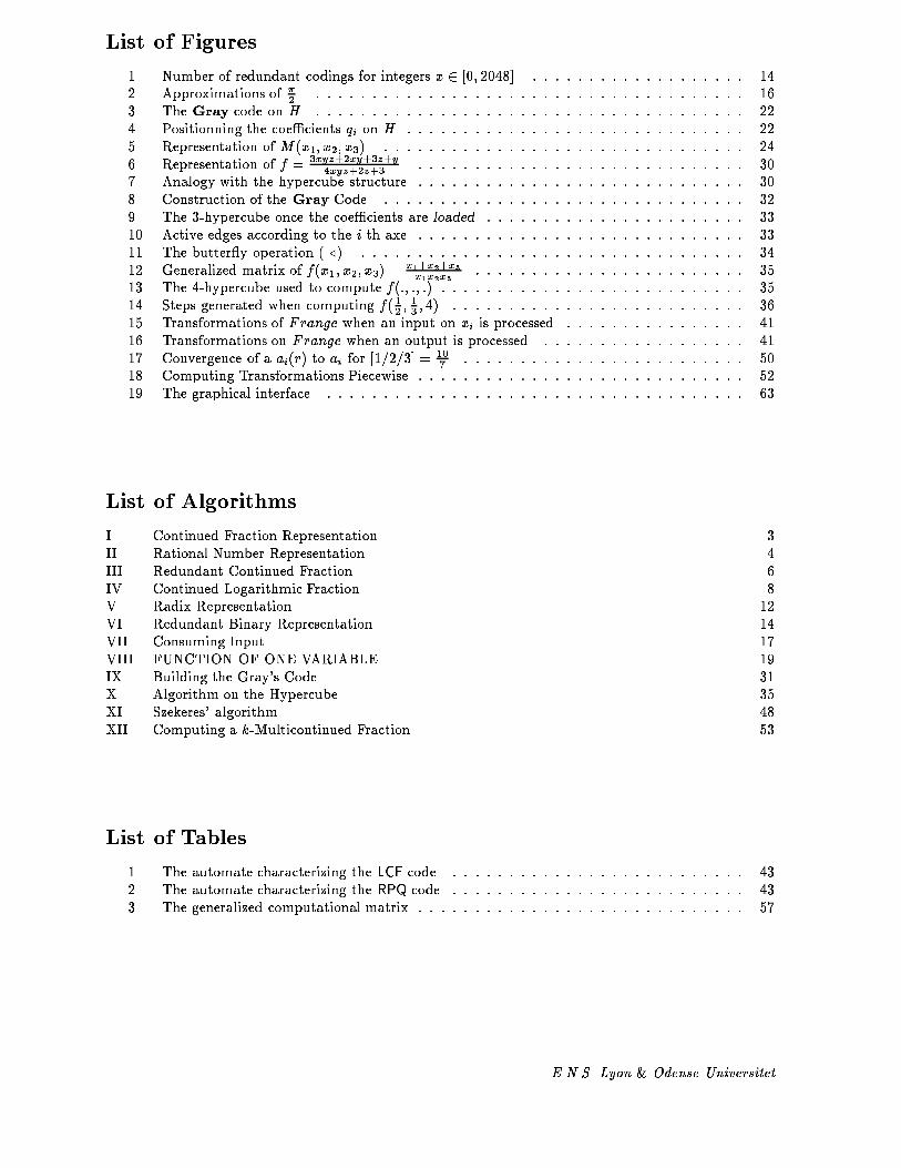
Algorithms on Continued Fractions 69List of Figures1 Number of redundant codings for integers x 2 [0; 2048]. : : : : : : : : : : : : : : : : : : : 142 Approximations of �2 . : : : : : : : : : : : : : : : : : : : : : : : : : : : : : : : : : : : : : : 163 The Gray code on H. : : : : : : : : : : : : : : : : : : : : : : : : : : : : : : : : : : : : : : 224 Positionning the coe�cients qi on H. : : : : : : : : : : : : : : : : : : : : : : : : : : : : : : 225 Representation of M (x1; x2; x3). : : : : : : : : : : : : : : : : : : : : : : : : : : : : : : : : 246 Representation of f = 3xyz+2xy+3z+y4xyz+2z+3 . : : : : : : : : : : : : : : : : : : : : : : : : : : : : : 307 Analogy with the hypercube structure. : : : : : : : : : : : : : : : : : : : : : : : : : : : : : 308 Construction of the Gray Code. : : : : : : : : : : : : : : : : : : : : : : : : : : : : : : : : 329 The 3-hypercube once the coe�cients are loaded. : : : : : : : : : : : : : : : : : : : : : : : 3310 Active edges according to the i-th axe. : : : : : : : : : : : : : : : : : : : : : : : : : : : : : 3311 The butter y operation (./). : : : : : : : : : : : : : : : : : : : : : : : : : : : : : : : : : : 3412 Generalized matrix of f(x1; x2; x3) = x1+x2+x3x1x2x3 . : : : : : : : : : : : : : : : : : : : : : : : : 3513 The 4-hypercube used to compute f(:; :; :) : : : : : : : : : : : : : : : : : : : : : : : : : : : 3514 Steps generated when computing f(12 ; 13 ; 4) : : : : : : : : : : : : : : : : : : : : : : : : : : 3615 Transformations of Frange when an input on xi is processed. : : : : : : : : : : : : : : : : 4116 Transformations on Frange when an output is processed. : : : : : : : : : : : : : : : : : : 4117 Convergence of a ai(r) to ai for [1=2=3] = 107 . : : : : : : : : : : : : : : : : : : : : : : : : : 5018 Computing Transformations Piecewise : : : : : : : : : : : : : : : : : : : : : : : : : : : : : 5219 The graphical interface. : : : : : : : : : : : : : : : : : : : : : : : : : : : : : : : : : : : : : 63List of AlgorithmsI Continued Fraction Representation . . . . . . . . . . . . . . . . . . . . . . . . 3II Rational Number Representation . . . . . . . . . . . . . . . . . . . . . . . . 4III Redundant Continued Fraction . . . . . . . . . . . . . . . . . . . . . . . . . 6IV Continued Logarithmic Fraction . . . . . . . . . . . . . . . . . . . . . . . . . 8V Radix Representation . . . . . . . . . . . . . . . . . . . . . . . . . . . . . 12VI Redundant Binary Representation . . . . . . . . . . . . . . . . . . . . . . . . 14VII Consuming Input . . . . . . . . . . . . . . . . . . . . . . . . . . . . . . . 17VIII FUNCTION OF ONE VARIABLE . . . . . . . . . . . . . . . . . . . . . . . . 19IX Building the Gray's Code . . . . . . . . . . . . . . . . . . . . . . . . . . . . 31X Algorithm on the Hypercube . . . . . . . . . . . . . . . . . . . . . . . . . . 35XI Szekeres' algorithm . . . . . . . . . . . . . . . . . . . . . . . . . . . . . . 48XII Computing a k-Multicontinued Fraction . . . . . . . . . . . . . . . . . . . . . 53List of Tables1 The automate characterizing the LCF code. : : : : : : : : : : : : : : : : : : : : : : : : : : 432 The automate characterizing the RPQ code. : : : : : : : : : : : : : : : : : : : : : : : : : : 433 The generalized computational matrix : : : : : : : : : : : : : : : : : : : : : : : : : : : : : 57E.N.S. Lyon & Odense Universitet

Algorithms on Continued Fractions 70References[1] William B. Jones, W.J. Thron Continued Fractions : Analytic Theory and Applications, Encyclope-dia of Mathematics And Its Applications, 1980 , Addison-Wesley.[2] Nicolaas H. Kuiper Linear Algebra and Geometry, 1965, North-Holland Publishing Compagny Am-sterdam.[3] Peter Kornerup, David W. Matula LCF: A lexicographic Binary Representation Of The Rationnals,April 1989, Odense Universitet.[4] Peter Kornerup, DavidW. Matula Exploiting Redundancy in Bit-Pipelined Rational Arithmetic, July1989, Odense Universitet.[5] Peter Kornerup, David W. Matula Finite Precision Lexicographic Continued Fraction Number Sys-tems, June 4-5 1985, IEEE COMPUTER SOCIETY.[6] Keld Antonsen, Kim Ramassen Analysis and Design of an On-line Arithmetic Unit, 1991, OdenseUniversitet.[7] Peter Kornerup, An On-line Arithmetic Unit for Bit-Pipelined Rational Arithmetic, 1987, Journalof Parallel and Distributed Computing.[8] Peter Kornerup, DavidW. MatulaAn Algorithm for Redundant Binary Bit-Pipelined Rational Arith-metic, August 1990, IEEE TRANSACTIONS ON COMPUTERS.[9] N.M. Blackman, The Continued Fraction as an Information Source, IEEE Trans.Inf.Th Vol. IT-30,1984,671-674[10] R.W. Gosper, item 101 in HAKMEM, MIT-AIM, Feb. 1972,37-44[11] G.H. Hardy and E.M. Wright, An Introduction to the Theory of Numbers 5th ed., Oxford UniversityPress, London, 1979[12] A.Y. Khintchin, Continued Fractions 1935[13] D.E. Knuth, Supernatural Numbers, in Mathematical Gardner, D.A. Klarner, ed., Van Nostrand,New-York, 1982 ,310-325[14] D.E. Knuth, The Art of Computer Programming, Vol. 2, Seminumerical Algorithms, 2nd Ed.,Addison-Wesley, reading, 1981.[15] T.W. Cusik, The Skezeres Multidimensional Continued Fraction, Mathematics of Computation, Vol-ume 31, Number 137, January 1977, Pages 280-317.[16] S�ren Peter Johansen, Specialet Ci�er-Seriel On-line Aritmetik, Institut for Matematik og Datalogi,Odense Universitet, August 1990, master project.E.N.S. Lyon & Odense Universitet