New Progress on FDC project

- Automatic deduction renormalization counter term

Jian-Xiong WangInstitute of High Energy Physics, Chinese Academy of Science, Beijing

IBS-KIAS Joint Workshop on Particle Physics, and CosmologyFeb. 5-10, 2017 High1, Resort, Korea

1 / 23

Introduction

It is well known that precision theoretical description on high energyphenomonolgy must be achieved.

Therefore, higher-order perturbative calculations in QFT for SM are requiredfor signal and background.

FDC project is aimed at automatic calculation on these calculation andalready can do next-leading-order(NLO) calculation automatically.

Based on FDC, there are already many hard works been achieved in last 8years.

Recent progress for FDC project will be introduced in this talk.

2 / 23

3 / 23

Introduction

The results are obtained analytically.

Two ways to generate square of amplitude:

Automatically phase space treatment

To automatically construct the Lagrangian and deduce the Feynman rulesfor SM, MSSM

First version of “FDC-LOOP” was completed by the end of 2007, used andimproved since then.

Many work on QCD correction are finished and published.

First version of FDC-PWA was completed on 2001 and improved 2003, usedby BES experimental group for partial-wave analysis

4 / 23

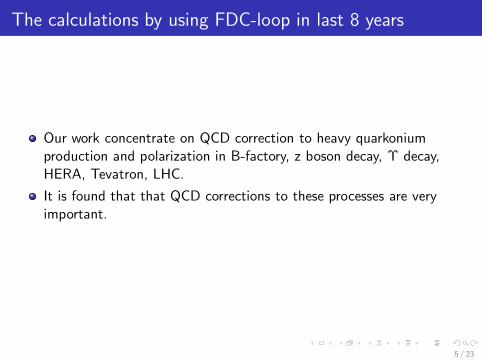
The calculations by using FDC-loop in last 8 years

Our work concentrate on QCD correction to heavy quarkoniumproduction and polarization in B-factory, z boson decay, Υ decay,HERA, Tevatron, LHC.

It is found that that QCD corrections to these processes are veryimportant.

5 / 23

Momentum distribution of J/ψ for e+e− → J/ψ+ gg at QCD NLO. PRL102, (2009) B. Gong and J. X. Wang

Pt distribution of J/ψ polarization at QCD NLO. PRL100,232001 (2008), B. Gong and J. X. Wang

6 / 23

QCD Correction to prompt J/ψ(3S11 ,

1S80 ,

3S81 ,

3P8J ) polarization

Figure: Polarization parameter λ of prompt J/ψ hadroproduction in helicity(left) and CS(right) frames.

PRL110, 042002, 2013, Bin Gong, Lu-Ping Wan, Jian-Xiong Wang and Hong-Fei Zhang

7 / 23

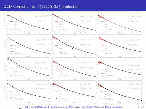
QCD Correction to Υ(1S , 2S , 3S) production

Figure:PRL 112, 032001, 2014, by Bin Gong, Lu-Ping Wan, Jian-Xiong Wang and Hong-Fei Zhang 8 / 23

QCD Correction to Υ(1S , 2S , 3S) polarization

Figure: Polarization parameter λ of prompt Υ(1S, 2S, 3S) hadroproduction in helicity frame

PRL 112, 032001, 2014, by Bin Gong, Lu-Ping Wan, Jian-Xiong Wang and Hong-Fei Zhang

9 / 23

Recent Progress in FDC project

New algorithm to construct and triangulate convex polyhedral coneand it’s application in higher order perturbative QFT calculation (Ipresented the talk on High1-2016 workshop)

automatic counter terms generation , automatic calculation ofrenormalization constant (This talk on High1-2017 workshop)

10 / 23

Tree-level Lagrangian construction and Feynman rules

generation

1994, Standard Model, 3 gauge group, 3 generation quark andleptons, more than 100 interaction vertices

2000, MSSM, 3 gauge group and suppersymmetry, 3 generation quarkand leptons with their supper partners, more than 5000 interactionvertices

2008, QCD one-loop counter term input by hand.

11 / 23

One-loop counter terms generation in last year

To construct counter terms and calculatioin all the renormalizationconstats for QCD or eletro-weak one-loop renormalization.

Very simple description input for first principle model with SU(n)gauge symmetry, such as the Standard Model, two-higgs doubletmodel, ....

Easy to add different matter fields

Different gauge can be easiy choosed, such as unitary gauge,Feynman-tohoft gauge, R-ksi Gauge, Landau gauge, ...

Different renormalization scheme, such as Keyto-scheme,European-scheme, On-shell or MS-bar scheme for QCDrenormalization choice.

For MSSM one-loop renormalization is still under construction.

Two-loop counter terms generation are under construction

12 / 23

13 / 23

14 / 23

15 / 23

16 / 23

%------------------------- Gauge fields ------------------------- gaugefields:= %No. Name SU(n) notation couping breaking '((1 u 1 b g1 yes ) (2 su 2 a g yes ) (3 su 3 gs g3 no ))$ %------------------------ Matter fields --------------------------- matterinput:={{name, 2*spin, chiral, 1, 2, 3}, { hig, 0 , rl , 1, 2, 0}, { el , 1, l , -1, 2, 0}, { er , 1, r , -2, 0, 0}, { q1l , 1, l , 1/3, 2, 3}, { q1dr, 1, r , -2/3, 0, 3}, { q1ur, 1, r , 4/3, 0, 3}}$ gauge_boson_redefine:={ a(1,~v) => (w(1,v)+w(-1,v))/2**0.5, a(2,~v) => (w(-1,v)-w(1,v))/2**0.5/i, a(3,~v) => z(0,v), b(~v) => p(0,v) }; vancumexpectation:='((hig v0)); % name n_group 1_componet 2_componet ... mdefl:={ {hig, 2, xx2 , (v0+h0-i*xx3)/2**0.5}, {el , 2, nue , ef }, {er , 2, ef }, {q1l , 2, qu , qd }, {q1dr, 2, qd }, {q1ur, 2, qu }}$

realfamily:='( (q1l q2l q3l) (q1dr q2dr q3dr) (q1ur q2ur q3ur) (qu qc qt) (qd qs qb) (el mul taul) (er mur taur) (ef mu tau) (nue numu nut)); phymass:={{w, wm}, {z, zm}, {p, 0}, {h0, hm}, {ef, fme}, {nue, 0},{mu, fmmu},{numu, 0},{tau, fmtau}, {nut, 0},{qd, fmd}, {qu, fmu},{qs, fms}, {qc, fmc}, {qb, fmb}, {qt, fmt}}$ phyinput:={g3,g,theta,wm, hm,fme, fmmu,fmtau,fmd, fmu,fms, fmc,fmb, fmt}$ construles:={ g1=>g*sin(theta)/cos(theta)}; expriment_easy_list:={ {g, replaceby, ge, -i*ge*gg(l,v), {p,ef,ef}}, {theta, replaceby, zm} }; charge_def:=tp(2,3)+tp(1,1)/2; renormalization:=‘before_broken; %European scheme %renormalization:=‘after_broken; %Kyoto scheme %ms_list:='(g3 ); symbolic(rform:='(1 2 )); symbolic(rloop:='((g . 2)));

Input file for Standard Model at electroweak NLO

17 / 23

fyl:={ {p, ksi1, sin(theta)*pd(a(3,v),v)+cos(theta)*pd(b(v),v),sin(theta)*(mutiplet(-1,2,hig,2,xx2(-1),(h0(0)+xx3(0)*i)/sqrt(2))*tp(1,2,2,3)*mutiplet(1,2,hig,2,0,v0/sqrt(2))*g*i-mutiplet(1,2,hig,2,0,v0 /sqrt(2))*tp(1,2,2,3)*mutiplet(1,2,hig,2,xx2(1),(h0(0)-xx3(0)*i)/sqrt(2))*g*i)/2+cos(theta)*(mutiplet(-1,2,hig,2,xx2(-1),(h0(0)+xx3(0)*i)/sqrt(2))*mutiplet(1,2,hig,2,0,v0/sqrt(2))*g1*i-mutiplet(-1,2,hig,2,0, v0/sqrt(2))*mutiplet(1,2,hig,2,xx2(1),(h0(0)-xx3(0)*i)/sqrt(2))*g1*i)/2, gh(-1,2,3)*sin(theta)+gh(-1,1)*cos(theta)}, {z, ksi2, cos(theta)*pd(a(3,v),v)+(-sin(theta))*pd(b(v),v),cos(theta)*(mutiplet(-1,2,hig,2,xx2(-1),(h0(0) +xx3(0)*i)/sqrt(2))*tp(1,2,2,3)*mutiplet(1,2,hig,2,0,v0/sqrt(2))*g*i-mutiplet(-1,2,hig,2,0,v0/sqrt(2))* tp(1,2,2,3)*mutiplet(1,2,hig,2,xx2(1),(h0(0)-xx3(0)*i)/sqrt(2))*g*i)/2+(-sin(theta))*(mutiplet(-1,2,hig, 2,xx2(-1),(h0(0)+xx3(0)*i)/sqrt(2))*mutiplet(1,2,hig,2,0,v0/sqrt(2))*g1*i-mutiplet(-1,2,hig,2,0,v0 /sqrt(2))*mutiplet(1,2,hig,2,xx2(1),(h0(0)-xx3(0)*i)/sqrt(2))*g1*i)/2, gh(-1,2,3)*cos(theta)-gh(-1,1)*sin(theta)}, {a(1), ksi3, pd(a(1,v),v),(mutiplet(-1,2,hig,2,xx2(-1),(h0(0)+xx3(0)*i)/sqrt(2))*tp(1,2,2,1)* mutiplet(1,2,hig,2,0,v0/sqrt(2))*g*i-mutiplet(-1,2,hig,2,0,v0/sqrt(2))*tp(1,2,2,1)*mutiplet(1,2,hig,2, xx2(1),(h0(0)-xx3(0)*i)/sqrt(2))*g*i)/2, gh(-1,2,1)}, {a(2), ksi3, pd(a(2,v),v),(mutiplet(-1,2,hig,2,xx2(-1),(h0(0)+xx3(0)*i)/sqrt(2))*tp(1,2,2,2)*mutiplet(1,2, hig,2,0,v0/sqrt(2))*g*i-mutiplet(-1,2,hig,2,0,v0/sqrt(2))*tp(1,2,2,2)*mutiplet(1,2,hig,2,xx2(1), (h0(0)-xx3(0)*i)/sqrt(2))*g*i)/2, gh(-1,2,2)}, {gs(ic10), ksi4 ,pd(gs(ic10,v),v),0, gsg(-1,ic10)}}$ r_ksi_value:='( (ksi1 . 1) (ksi2 . 1) (ksi3 . 1) (ksi4 . 1))$ %Default Feynman-tohoft gaige end$

Generatetd File: “gauge_fix_term” Can be used to choose different Gague

18 / 23

fyl:={ {p, ksi1, sin(theta)*pd(a(3,v),v)+cos(theta)*pd(b(v),v),sin(theta)*(mutiplet(-1,2,hig,2,xx2(-1),(h0(0)+xx3(0)*i)/sqrt(2))*tp(1,2,2,3)*mutiplet(1,2,hig,2,0,v0/sqrt(2))*g*i-mutiplet(1,2,hig,2,0,v0 /sqrt(2))*tp(1,2,2,3)*mutiplet(1,2,hig,2,xx2(1),(h0(0)-xx3(0)*i)/sqrt(2))*g*i)/2+cos(theta)*(mutiplet(-1,2,hig,2,xx2(-1),(h0(0)+xx3(0)*i)/sqrt(2))*mutiplet(1,2,hig,2,0,v0/sqrt(2))*g1*i-mutiplet(-1,2,hig,2,0, v0/sqrt(2))*mutiplet(1,2,hig,2,xx2(1),(h0(0)-xx3(0)*i)/sqrt(2))*g1*i)/2, gh(-1,2,3)*sin(theta)+gh(-1,1)*cos(theta)}, {z, ksi2, cos(theta)*pd(a(3,v),v)+(-sin(theta))*pd(b(v),v),cos(theta)*(mutiplet(-1,2,hig,2,xx2(-1),(h0(0) +xx3(0)*i)/sqrt(2))*tp(1,2,2,3)*mutiplet(1,2,hig,2,0,v0/sqrt(2))*g*i-mutiplet(-1,2,hig,2,0,v0/sqrt(2))* tp(1,2,2,3)*mutiplet(1,2,hig,2,xx2(1),(h0(0)-xx3(0)*i)/sqrt(2))*g*i)/2+(-sin(theta))*(mutiplet(-1,2,hig, 2,xx2(-1),(h0(0)+xx3(0)*i)/sqrt(2))*mutiplet(1,2,hig,2,0,v0/sqrt(2))*g1*i-mutiplet(-1,2,hig,2,0,v0 /sqrt(2))*mutiplet(1,2,hig,2,xx2(1),(h0(0)-xx3(0)*i)/sqrt(2))*g1*i)/2, gh(-1,2,3)*cos(theta)-gh(-1,1)*sin(theta)}, {a(1), ksi3, pd(a(1,v),v),(mutiplet(-1,2,hig,2,xx2(-1),(h0(0)+xx3(0)*i)/sqrt(2))*tp(1,2,2,1)* mutiplet(1,2,hig,2,0,v0/sqrt(2))*g*i-mutiplet(-1,2,hig,2,0,v0/sqrt(2))*tp(1,2,2,1)*mutiplet(1,2,hig,2, xx2(1),(h0(0)-xx3(0)*i)/sqrt(2))*g*i)/2, gh(-1,2,1)}, {a(2), ksi3, pd(a(2,v),v),(mutiplet(-1,2,hig,2,xx2(-1),(h0(0)+xx3(0)*i)/sqrt(2))*tp(1,2,2,2)*mutiplet(1,2, hig,2,0,v0/sqrt(2))*g*i-mutiplet(-1,2,hig,2,0,v0/sqrt(2))*tp(1,2,2,2)*mutiplet(1,2,hig,2,xx2(1), (h0(0)-xx3(0)*i)/sqrt(2))*g*i)/2, gh(-1,2,2)}, {gs(ic10), ksi4 ,pd(gs(ic10,v),v),0, gsg(-1,ic10)}}$ r_ksi_value:='( (ksi1 . infinit) (ksi2 . infinit) (ksi3 . infinit) (ksi4 . 1))$ %Unitary Gauge end$

Generatetd File: “gauge_fix_term” Can be used to choose different Gague

19 / 23

%------------------------- Gauge fields ------------------------- gaugefields:= %No. Name SU(n) notation couping breaking '((1 u 1 b g1 yes ) (2 su 2 a g yes ) (3 su 3 gs g3 no ))$ %------------------------ Matter fields --------------------------- matterinput:={{name, 2*spin, chiral, 1, 2, 3}, { hig, 0 , rl , 1, 2, 0}, { el , 1, l , -1, 2, 0}, { er , 1, r , -2, 0, 0}, { q1l , 1, l , 1/3, 2, 3}, { q1dr, 1, r , -2/3, 0, 3}, { q1ur, 1, r , 4/3, 0, 3}}$ gauge_boson_redefine:={ a(1,~v) => (w(1,v)+w(-1,v))/2**0.5, a(2,~v) => (w(-1,v)-w(1,v))/2**0.5/i, a(3,~v) => z(0,v), b(~v) => p(0,v) }; vancumexpectation:='((hig v0)); % name n_group 1_componet 2_componet ... mdefl:={ {hig, 2, xx2 , (v0+h0-i*xx3)/2**0.5}, {el , 2, nue , ef }, {er , 2, ef }, {q1l , 2, qu , qd }, {q1dr, 2, qd }, {q1ur, 2, qu }}$

realfamily:='( (q1l q2l q3l) (q1dr q2dr q3dr) (q1ur q2ur q3ur) (qu qc qt) (qd qs qb) (el mul taul) (er mur taur) (ef mu tau) (nue numu nut)); phymass:={{w, wm}, {z, zm}, {p, 0}, {h0, hm}, {ef, fme}, {nue, 0},{mu, fmmu},{numu, 0},{tau, fmtau}, {nut, 0},{qd, fmd}, {qu, fmu},{qs, fms}, {qc, fmc}, {qb, fmb}, {qt, fmt}}$ phyinput:={g3,g,theta,wm, hm,fme, fmmu,fmtau,fmd, fmu,fms, fmc,fmb, fmt}$ construles:={ g1=>g*sin(theta)/cos(theta)}; expriment_easy_list:={ {g, replaceby, ge, -i*ge*gg(l,v), {p,ef,ef}}, {theta, replaceby, zm} }; charge_def:=tp(2,3)+tp(1,1)/2; renormalization:=‘before_broken; %European scheme %renormalization:=‘after_broken; %Kyoto scheme ms_list:='(g3 ); symbolic(rform:='(3)); symbolic(rloop:='((g3 . 2)));

Input file for Standard Model at QCD NLO by using onshell scheme

20 / 23

%------------------------- Gauge fields ------------------------- gaugefields:= %No. Name SU(n) notation couping breaking '((1 u 1 b g1 yes ) (2 su 2 a g yes ) (3 su 3 gs g3 no ))$ %------------------------ Matter fields --------------------------- matterinput:={{name, 2*spin, chiral, 1, 2, 3}, { hig, 0 , rl , 1, 2, 0}, { el , 1, l , -1, 2, 0}, { er , 1, r , -2, 0, 0}, { q1l , 1, l , 1/3, 2, 3}, { q1dr, 1, r , -2/3, 0, 3}, { q1ur, 1, r , 4/3, 0, 3}}$ gauge_boson_redefine:={ a(1,~v) => (w(1,v)+w(-1,v))/2**0.5, a(2,~v) => (w(-1,v)-w(1,v))/2**0.5/i, a(3,~v) => z(0,v), b(~v) => p(0,v) }; vancumexpectation:='((hig v0)); % name n_group 1_componet 2_componet ... mdefl:={ {hig, 2, xx2 , (v0+h0-i*xx3)/2**0.5}, {el , 2, nue , ef }, {er , 2, ef }, {q1l , 2, qu , qd }, {q1dr, 2, qd }, {q1ur, 2, qu }}$

realfamily:='( (q1l q2l q3l) (q1dr q2dr q3dr) (q1ur q2ur q3ur) (qu qc qt) (qd qs qb) (el mul taul) (er mur taur) (ef mu tau) (nue numu nut)); phymass:={{w, wm}, {z, zm}, {p, 0}, {h0, hm}, {ef, fme}, {nue, 0},{mu, fmmu},{numu, 0},{tau, fmtau}, {nut, 0},{qd, fmd}, {qu, fmu},{qs, fms}, {qc, fmc}, {qb, fmb}, {qt, fmt}}$ phyinput:={g3,g,theta,wm, hm,fme, fmmu,fmtau,fmd, fmu,fms, fmc,fmb, fmt}$ construles:={ g1=>g*sin(theta)/cos(theta)}; expriment_easy_list:={ {g, replaceby, ge, -i*ge*gg(l,v), {p,ef,ef}}, {theta, replaceby, zm} }; charge_def:=tp(2,3)+tp(1,1)/2; renormalization:=‘before_broken; %European scheme %renormalization:=‘after_broken; %Kyoto scheme ms_list:='(g3 gs qu qb qt qs qd qc); symbolic(rform:='(3)); symbolic(rloop:='((g3 . 2)));

Input file for Standard Model at QCD NLO by using MS_bar scheme

21 / 23

Summary

22 / 23

Thanks for your attention!

23 / 23