Neural Networks 139 (2021) 305–325

stsldawSeau

h0

Contents lists available at ScienceDirect

Neural Networks

journal homepage: www.elsevier.com/locate/neunet

CiwGAN and fiwGAN: Encoding information in acoustic data tomodellexical learningwith Generative Adversarial NetworksGašper BegušDepartment of Linguistics, University of California, Berkeley, United States of America

a r t i c l e i n f o

Article history:Available online 19 March 2021

Keywords:Artificial intelligenceGenerative adversarial networksSpeechLexical learningNeural network interpretabilityAcoustic word embedding

a b s t r a c t

How can deep neural networks encode information that corresponds to words in human speech intoraw acoustic data? This paper proposes two neural network architectures for modeling unsupervisedlexical learning from raw acoustic inputs: ciwGAN (Categorical InfoWaveGAN) and fiwGAN (FeaturalInfoWaveGAN). These combine Deep Convolutional GAN architecture for audio data (WaveGAN;Donahue et al., 2019) with the information theoretic extension of GAN – InfoGAN (Chen et al., 2016)– and propose a new latent space structure that can model featural learning simultaneously with ahigher level classification and allows for a very low-dimension vector representation of lexical items.In addition to the Generator and Discriminator networks, the architectures introduce a network thatlearns to retrieve latent codes from generated audio outputs. Lexical learning is thus modeled asemergent from an architecture that forces a deep neural network to output data such that uniqueinformation is retrievable from its acoustic outputs. The networks trained on lexical items fromthe TIMIT corpus learn to encode unique information corresponding to lexical items in the formof categorical variables in their latent space. By manipulating these variables, the network outputsspecific lexical items. The network occasionally outputs innovative lexical items that violate trainingdata, but are linguistically interpretable and highly informative for cognitive modeling and neuralnetwork interpretability. Innovative outputs suggest that phonetic and phonological representationslearned by the network can be productively recombined and directly paralleled to productivity inhuman speech: a fiwGAN network trained on suit and dark outputs innovative start, even though itnever saw start or even a [st] sequence in the training data. We also argue that setting latent featuralcodes to values well beyond training range results in almost categorical generation of prototypicallexical items and reveals underlying values of each latent code. Probing deep neural networks trainedon well understood dependencies in speech bears implications for latent space interpretability andunderstanding how deep neural networks learn meaningful representations, as well as potential forunsupervised text-to-speech generation in the GAN framework.

© 2021 The Author. Published by Elsevier Ltd. This is an open access article under the CC BY license(http://creativecommons.org/licenses/by/4.0/).

1. Introduction

How human language learners encode information in theirpeech is among the core questions in linguistics and compu-ational cognitive science. Acoustic speech data is the primaryource of linguistic input for hearing infants, and first languageearners must learn to retrieve information from raw acousticata. By the time language acquisition is complete, learners areble to not only analyze but also produce speech consisting ofords (henceforth lexical items) that carry meaning (Kuhl, 2010;affran et al., 1996, 2007). In other words, speakers learn toncode information in their acoustic output, and they do so byssociating meaning-bearing units of speech (lexical items) withnique information. Lexical items in turn consist of units called

E-mail address: begus@berkeley.edu.

ttps://doi.org/10.1016/j.neunet.2021.03.017893-6080/© 2021 The Author. Published by Elsevier Ltd. This is an open access arti

phonemes that represent individual sounds. In fact, speakers notonly produce lexical items that exist in their primary linguis-tic data, but are also able to generate new lexical items thatconsist of novel combinations of phonemes that conform to thephonotactic rules of their language. This points to one of the coreproperties of language: productivity (Baroni, 2020; Hockett, 1959;Piantadosi & Fedorenko, 2017).

1.1. Prior work

Computational approaches to lexical learning have a long his-tory. Modeling lexical learning can take many forms (for a com-prehensive overview, see Räsänen, 2012), but the shift towardsmodeling lexical learning from acoustic data, especially from rawunreduced acoustic data, has occurred relatively recently (Baayen

et al., 2019; Chorowski et al., 2019; Chung et al., 2016; Kamper,

cle under the CC BY license (http://creativecommons.org/licenses/by/4.0/).

G. Beguš Neural Networks 139 (2021) 305–325

2Boffa22eS

ldwailT

019; Lee et al., 2015; Levin et al., 2013; Shafaei-Bajestan &aayen, 2018, i.a.). Previously, the majority of models operatedn either fully abstracted or already simplified features extractedrom raw acoustic data. A variety of models have been proposedor this task including, among others, Bayesian and connectionistpproaches (see, among others Arnold et al., 2017; Baayen et al.,019; Chuang et al., 2020; Elsner et al., 2013; Feldman et al.,013, 2009; Goldwater et al., 2009; Heymann et al., 2013; Kampert al., 2017; Lee & Glass, 2012; Lee et al., 2015; Räsänen, 2012;hafaei-Bajestan & Baayen, 2018).As summarized in Lee et al. (2015), existing models of lexical

earning that take some form of acoustic data as input can beivided into ‘‘spoken term discovery’’ models and ‘‘models oford segmentation’’ (Lee et al., 2015, 390). Proposals of the firstpproach most commonly involve the clustering of similaritiesn acoustic data to establish a set of phonetic units from whichexical items are then established, again based on clustering.he word segmentation models, on the other hand, ‘‘start from

unsegmented strings of symbols and attempt to identify subse-quences corresponding to lexical items’’ (Lee et al., 2015, 390; forevaluation of the models, see also Levin et al., 2013). The modelscan take as inputs acoustic data pre-segmented at the word level(as in the current paper and Chung et al., 2016; Kamper et al.,2014) or acoustic inputs of unsegmented speech (e.g. in Lee et al.,2015; Räsänen & Blandón, 2020; Räsänen et al., 2015).

Weakly supervised and unsupervised deep neural networkmodels operating on acoustic data have recently been used tomodel phonetic learning (Alishahi et al., 2017; Chung et al., 2020;Eloff et al., 2019; Räsänen et al., 2016; Shain & Elsner, 2019), butnot learning of phonological processes. Evidence for phonemicrepresentation in deep neural networks, for example, emergesin a weakly supervised model that combines visual and auditoryinformation (Alishahi et al., 2017). Several prominent autoen-coder models that are trained to represent data in a lower-dimensionality space have recently been proposed (Chorowskiet al., 2019; Eloff et al., 2019; Räsänen et al., 2016; Shain & Elsner,2019). Clustering analyses of the reduced space in these autoen-coder models suggest that the networks learn approximates tophonetic features. The disadvantage of the autoencoder archi-tecture is that outputs reproduce inputs as closely as possible:the network’s outputs are directly connected to its inputs, whichis not an ideal setting for language acquisition. Furthermore,current proposals in the autoencoder framework do not modelphonological processes, and there is only an indirect relationshipbetween phonetic properties and latent space.

A prominent framework for modeling lexical learning is acous-tic word embedding models that include various (mostly un-supervised) methods (Kamper et al., 2014; Levin et al., 2013)including deep neural networks (Baevski et al., 2020; Chunget al., 2016; Hu et al., 2020; Niekerk et al., 2020). Similar tothe phone-level autoencoder models, the goal of the acousticword embedding models is a parsimonious encoding of lexicalitems that maps acoustic input into a fixed dimensionality vec-tor (Chung et al., 2016; Levin et al., 2013). The models can beused for unsupervised lexical learning and spoken term discoveryin low resource languages (e.g. the Zerospeech challenge; Dunbaret al., 2019, 2017, 2020). Several models within this frameworkemploy the autoencoder architecture, where the latent spacereduced in dimensionality can serve as a vector representingacoustic lexical items (Chung et al., 2016; Kamper, 2019; Niek-erk et al., 2020). Chung et al. (2016) show that averaged latentrepresentations can correspond to phonetic representations, butin order to get these results they additionally perform dimen-sionality reduction on the latent space. Similarly, Chorowski et al.(2019) use a vector quantized variational autoencoder (VQ-VAE)in which the encoder outputs categorical values constituting to-ken identity. Chorowski et al. (2019) argue that token identities

306

match phoneme identities with relative high frequencies (seealso Chung et al., 2020; Niekerk et al., 2020). Chen and Hain(2020) argue that a convolutional encoder outputs a higher qual-ity of audio compared to the RNN architectures that most of thementioned proposals use.

One of the major contributions of these models is the facil-itation of unsupervised automatic speech recognition (ASR) forzero resource languages, which is why their evaluation focuses onmetrics such as the word discrimination/error tasks (e.g. Baevskiet al., 2020; Chen & Hain, 2020; Chung et al., 2016; Kamper,2019; Levin et al., 2013; Niekerk et al., 2020) or naturalness of theoutputs (e.g. Chen & Hain, 2020; Eloff et al., 2019; Niekerk et al.,2020). A subset of proposals explores interpretability of the latentspace and generated outputs (see Chorowski et al., 2019; Chunget al., 2016), but they focus on the entire latent space ratherthan on individual variables or their direct influence on generatedoutputs. Moreover, the acoustic word embedding models stilloperate with relatively high dimensional vectors (substantiallyhigher than in the fiwGAN architecture; see Section 3.4) and theirinterpretation often includes the entire latent vector or requiresadditional dimensionality reduction techniques. To my knowl-edge, exploration of how individual variables in these vectorscorrespond to linguistically meaningful units or how we can elicitcategorical behavior (see Section 3.3.2) is absent.

Finally, while autoencoders are generative and unsupervised,they crucially differ from GANs in that the encoder does havedirect access to the data. Additionally, autoencoders are trainedon replicating data rather than on learning to generate data fromnoise in an unsupervised manner. In other words, autoencodersare unsupervised in terms of encoding data representations in thelatent space, but the data generation part (decoders) is supervisedin the autoencoder architecture. GANs, on the other hand, areunsupervised also in the sense of data generation. This distinctionis primarily relevant for the cognitive modeling aspect of theproposal.

The ideal cognitive model of lexical learning would includeboth the production and the perception aspect. Here we focuson evaluating generated outputs and on the interpretability ofthe latent space; we leave the question of how the Q-networkperforms on lexical item identification/discrimination for futurework. This brings some limitations in terms of model comparison— we lack information on how well a GAN-based unsupervisedlexical learner performs on word discrimination tasks comparedto, for example, the autoencoder architecture. It is reasonable toassume that GAN-based models would perform worse on worddiscrimination tasks compared to autoencoders in which both theencoder and decoder have direct access to the training data. TheGenerator and the Q-network in the proposed architecture do nothave a direct access to the training data — the Generator has onlya very indirect access to the data by being trained on maximizingthe error of the Discriminator that aims to estimate Wassersteindistance between generated and real data. Additionally, the fiw-GAN and ciwGAN models proposed here have substantially morereduced latent representations (from 5 to 13 variables total). Thislikely negatively affects the word discrimination, and as such, theevaluation of discrimination is left for future work.

Another advantage of the GAN architecture is that the net-works generate innovative data rather than replicates of data. Wecan thus probe learning by analyzing how GANs innovate, howthey violate data distributions, and what can these innovativeoutputs tell us about their learning. Additionally, we focus on ex-ploring how manipulating the latent space (as proposed in Beguš,2020a) can elicit generation of unique lexical items at categoricallevels, what effects individual latent variables have on outputs,and what this manipulation can tell us about lexical learning in

deep convolutional networks.

G. Beguš Neural Networks 139 (2021) 305–325

1

eirvtecitDGidvaiWfIgb

btvfpavptmttn

tdnWptkipsswdbGigEipwe

phtaohl

.2. GANs and language acquisition

The main characteristics of the GAN architecture (Goodfellowt al., 2014) are two networks: the Generator and the Discrim-nator. The Generator generates data from latent space that iseduced in dimensionality (e.g. from a set of uniformly distributedariables z). The Discriminator network learns to distinguish be-ween ‘‘real’’ training data and generated outputs from the Gen-rator network. The Generator is trained to maximize the Dis-riminator’s error rate; the Discriminator is trained to minimizets own error rate. In the DCGAN proposal (Radford et al., 2015),he two networks are deep convolutional networks. Recently, theCGAN proposal was transformed to model audio data in Wave-AN (Donahue et al., 2019). The main architecture of WaveGANs identical to that of DCGAN (Radford et al., 2015), with the mainifference being that the Generator outputs a one-dimensionalector corresponding to time series data (raw acoustic output)nd the Discriminator takes one-dimensional acoustic data as itsnput (as opposed to two-dimensional visual data in DCGAN).aveGAN also adopts the Wasserstein GAN proposal for a cost

unction in GANs that improves training (Arjovsky et al., 2017).nstead of estimating the probability of whether the output isenerated or real, WGAN estimates the Wasserstein distanceetween generated data and real data.Beguš (2020a) models speech acquisition as a dependency

etween latent space and generated outputs in the GAN archi-ecture. The paper proposes a technique for identifying latentariables that correspond to meaningful phonetic/phonologicaleatures in the output. The Generator network learns to encodehonetically and phonologically meaningful representations, suchs the presence of a segment in the output, with a subset ofariables, i.e. with reduced representation. Using the techniqueroposed in Beguš (2020a), we can identify individual variableshat correspond to, for example, a sound [s] in the output. Byanipulating these identified variables to values that are beyond

he training range, we can force [s] in the output. Interpolatinghe values has an almost linear effect on the amplitude of fricationoise of [s] in the output.One of the advantages of the proposal in Beguš (2020a) is

hat the model learns phonological alternations, i.e. context-ependent changes in the realization of speech sounds, simulta-eously with learning acoustic properties of human speech. TheaveGAN model (Donahue et al., 2019) is trained on a simplehonological process: aspiration of stops /p, t, k/ conditioned onhe presence of [s] in the input. English voiceless stops /p, t,/ are aspirated (produced with a puff of air [ph, th, kh]) word-nitially before a stressed vowel (e.g. in pit ["phIt]) except if an [s]recedes the stop (e.g. spit ["spIt]) A computational experimentuggests that the network learns this distribution, but imperfectlyo. The network learns to output shorter aspiration durationhen [s] is present, in line with distributions in the trainingata. Outputs, however, also violate data in a manner that cane directly paralleled to language acquisition. Occasionally, theenerator network outputs aspiration durations that are longern the [s] condition than in any example in the training data: theenerator outputs [sphIt], which violates the phonological rule innglish. In other words, the network violates the distributionsn the training data, and these violations correspond directly tohonological acquisition stages: children acquiring English startith significantly longer aspiration durations in the [s]-condition,.g. [sphIt] (Bond & Wilson, 1980).In sum, GANs have been shown to represent phonetically or

honologically meaningful information in the latent space thatas approximate equivalent in phonetic/phonological represen-ations and language acquisition (Beguš, 2020a). The latent vari-bles can be actively manipulated to generate data with or with-ut some phonetic/phonological property. These representations,owever, are exclusively limited to the phonetic/phonologicalevel in Beguš (2020a) and contain no lexical information.

p

307

1.3. Goals

Despite several advantages, to our knowledge, lexical learninghas not yet been modeled with Generative Adversarial Neuralnetwork models and perhaps even more generally, with unsu-pervised generative deep convolutional networks. Donahue et al.(2019) train the WaveGAN architecture on Speech CommandsZero Through Nine (SC09) dataset and argues that the networklearns to generate speech-like outputs with high naturalness andinception scores. Donahue et al. (2019), however, do not exploreinternal representations and their architecture does not includethe Q-network (InfoGAN; Chen et al., 2016), which means theproposal does not model lexical learning or how the networkencodes linguistically meaningful representations. As discussedin Section 1.1, most other models operate with recurrent neuralnetworks rather than with convolutional networks and use theautoencoder architecture.1

In this paper, we follow the proposal in Beguš (2020a) thatphonetic and phonological acquisition can be modeled as a de-pendency between latent space and generated data in the GANarchitecture and add a lexical learning component to the model.We modify the WaveGAN architecture and add the InfoGAN’s Q-network (based partially on implementation in Rodionov, 2018)to computationally simulate lexical learning from raw acousticdata. In other words, we introduce a deep convolutional networkthat learns to retrieve the Generator’s latent code and proposea new latent space structure that can model featural learning(fiwGAN). The fiwGAN architecture additionally allows a verylow dimension categorical vector representation of lexical items(e.g. n number of features allows 2n number of unique classes).We train the networks on highly variable training data: manuallysliced lexical items from the TIMIT database (Garofolo et al.,1993) that includes over 600 speakers from different dialectalbackgrounds in American English. We present four computationalexperiments: on five lexical items in the ciwGAN architecture(Section 3.1), on ten lexical items in the ciwGAN architecture(Section 3.2), on eight lexical items in the fiwGAN architecture(Section 3.3), and on the entire TIMIT database (6,229 lexicalitems) in the fiwGAN architecture (Section 3.4). Evidence forlexical learning emerges in all four experiments. The paper alsofeatures a section describing how to directly follow learningstrategies of the Generator network (Section 3.1.2), a section onfeatural learning that discusses innovative outputs and produc-tivity of the model (Section 3.3.1), and a section that proposes atechnique for retrieving near categorical underlying representa-tion of the latent variables in GANs (Section 3.3.2). We argue thatexploration of innovative outputs and the latent space of deepneural networks trained on dependencies on speech data that arewell understood (due to extensive study of human phonetics andphonology in the past decades) provides unique insights both forcognitive modeling and for neural network interpretability.

Lexical learning is modeled in the following way: a deepconvolutional network learns to retrieve information from inno-vative outputs generated by a separate Generator network. TheGenerator network thus learns to generate data such that uniquelexical information is retrievable from its acoustic outputs. Lexicallearning is not per se incorporated in the model: instead, lexicallearning emerges because the most informative way to generateoutputs given speech data as input is to encode unique informa-tion into lexical items. The end result of the model is a Generatornetwork that generates innovative data – raw acoustic outputs– such that each lexical item is represented by a unique code.Because the model diverges substantially from existing proposals

1 A deep convolutional autoencoder model architecture based on WaveNetroposed in Chen and Hain (2020) was released after submission of this paper.

G. Beguš Neural Networks 139 (2021) 305–325

o(ewr

ciawlewwa1

drfpierititir(tdgfTiihars

potbtmilmt

epBiuastrwtnuGc

Ifu

f lexical learning, we leave direct comparison of its performancesuch as on ABX test) for future work. Instead, we propose tovaluate success in the model’s performance in lexical learningith an inferential statistical technique — multinomial logisticegression (Section 3.1).

Representing semantic information can take many forms inomputational models. In the current proposal, unique lexicaltems are represented with either a one-hot vector in the ciwGANrchitecture or a binary code in the fiwGAN architecture. In otherords, the objective of the model is to associate each unique

exical item in the training data with a unique representation. Forxample, in a corpus with four words, word1 can be associatedith a representation [1, 0, 0, 0], word2 with [0, 1, 0, 0], word3ith [0, 0, 1, 0] in the ciwGAN architecture. In the fiwGANrchitecture, word1 can be associated with [0, 0], word2 with [0,], word3 with [1, 0], and word4 with [1, 1].The model of lexical learning proposed here features some

esirable properties. First, the network is trained exclusively onaw unannotated acoustic data. Second, lexical learning emergesrom the requirement on a deep convolutional network to out-ut informative data. Only because associating a unique coden the latent space with lexical items is the optimal way toncode information such that another network will be able toetrieve it does the lexical learning emerge. Third, the models fully generative: a deep convolutional network (the Genera-or) generates raw acoustic outputs that correspond to lexicaltems in the training data. Crucially, the Generator network inhe model does not simply replicate training data, but generatesnnovative outputs, because its main task is to increase the errorate of the network that distinguishes real from generated datathe Discriminator) and its outputs are not directly connected tohe training data. Occasionally, the Generator outputs innovativeata that violate distributions of the training data, but are lin-uistically interpretable and highly informative. The model thuseatures one of the basic properties of language: productivity.his allows us to compare lexical and phonological acquisitionn language-acquiring children to the innovative generated datan the proposed computational model. The fiwGAN architectureas an additional advantage: it can model featural learning inddition to a higher level classification. This means that featu-al representations in phonology and phonetics can be modeledimultaneously with lexical learning.To be sure, there are also undesirable aspects of the model. In

articular, the model’s performance is optimal when the numberf lexical classes that the network is predetermined. However, ashe experiment in Section 3.4 suggests, even with the mismatchetween the number of classes and the number of unique items,he networks show evidence for lexical learning. Also, while theodel learns from raw acoustic inputs, the individual lexical

tems in training data are sliced from the corpus (sliced at theexical level rather on the phone level) instead of inferred by theodel. These disadvantages are not insurmountable, but are left

o be addressed in future work.The proposed architectures and results of the computational

xperiments have implications for deep neural network inter-retability as well as some basic implications for NLP applications.eside modeling lexical learning, the novel latent space structuren the fiwGAN architecture can be employed as a general purposensupervised simultaneous feature extractor and classifier forudio data. We also propose a technique for exploring latentpace representations: we argue that manipulating latent codeso marginal values that substantially excess the training rangeeveals underlying values for each latent code. Outputs generatedith the proposed technique feature little variability and havehe potential to reveal learning representations of the Generatoretwork. The proposed model also allows a first step towardsnsupervised text-to-speech synthesis at the lexical level usingANs: the Generator outputs specific lexical items when latentodes are set to different values.

Q

308

2. Model

We propose a GAN architecture that combines WaveGAN withthe InfoGAN proposal (Chen et al., 2016). The objective of Genera-tive Adversarial Networks is a function that maps from randomly-distributed latent space to outputs that resemble training data(the Generator network). To find such a function, the Generatorand the Discriminator networks are trained in a minimax gamein which the Discriminator’s (D) loss is maximized and the Gen-erator’s (G) loss is minimized (Goodfellow et al., 2014). In theoriginal GAN proposal (Goodfellow et al., 2014), the Discriminatoris trained on classifying real and fake data. In the WassersteinGAN proposal that is adopted in this paper (as well as in Don-ahue et al., 2019) and that substantially improves training, theDiscriminator is trained on minimizing the Wasserstein distancebetween the generated and real data distributions (Arjovsky et al.,2017). The value function can be formalized as (Arjovsky et al.,2017; Donahue et al., 2019):

VWGAN (D,G) = Ex∼PX [Dw(x)] − Ez∼PZ [Dw(G(z))], (1)

where x is real data from some data distribution (PX ) and z islatent space from a random distribution (PZ ; in our case the uni-form distribution). To improve performance, the models are addi-tionally trained with a gradient penalty term λEx̂∼Px̂[(∥▽x̂Dw(x̂)∥2−1)2], where Px̂ is a uniform probability distributionin the interval [0, 1] which is used to sample from the differencebetween the real and generated data distributions (x̂) to get thegradient penalty and λ is a constant set at 10 (for advantagesof such a gradient penalty term over weight clipping, see theWGAN-GP proposal in Gulrajani et al., 2017).

InfoGAN (Chen et al., 2016) is a proposal within the GANframework that aims to increase mutual information betweena subset of latent space – the code variables (c or φ) – andgenerated outputs (G(z, c)) (Chen et al., 2016). In this paper, weadopt the main objectives from the Wasserstein proposal (1) andadd to the model maximization of mutual information betweenthe code variables in the latent space and the generated outputsI(c;G(z, c)). Because I(c;G(z, c)) is difficult to estimate, Chenet al. (2016) instead propose to approximate its variational lowerbound λLI (G,Q ) (with a hyperparameter λ; for details, see Chenet al., 2016). Our model can thus be formalized as (based on Chenet al., 2016 and Gulrajani et al., 2017; see also (1)):

minG,Q

maxD

VIWGAN (D,G,Q ) = VWGAN (D,G) − λLI (G,Q ). (2)

To implement this model, the proposed ciwGAN and fiw-GAN architectures involve three deep convolutional networks:the Generator, the Discriminator, and the Q-network (or the lex-ical learner). The models are based on WaveGAN (Donahue et al.,2019), an implementation of the DCGAN architecture (Radfordet al., 2015) for audio data and the InfoGAN proposal (Chen et al.,2016).2 Unlike in most InfoGAN implementations, the Q-networkis a separate deep convolutional network.3

In the GAN architecture, the Generator network usually takesas its input a number of uniformly distributed latent variables(z ∼ U(−1, 1)). In the InfoGAN proposal (Chen et al., 2016),the Generator’s input additionally includes a latent code: a setof binary variables that constitutes a one-hot vector as well asuniformly distributed code variables. Because we model lexicallearning, we exclude uniformly distributed code variables. While

2 Barry and Kim (2019) in a recent presentation model piano playing withnfoWaveGAN. Their proposal, however, focuses on continuous variables andeature only one categorical latent variable with no apparent function. It isnclear from the poster what the architecture of their proposal is.3 The InfoGAN model based on DCGAN in Rodionov (2018) also proposes the-network to be a separate network.

G. Beguš Neural Networks 139 (2021) 305–325

ttc(atvftosatntvouac

wvajTtifed‘tiDo

tQpatftiisDidlQngl

ocsocQc

i

ents

he binary variables in InfoGAN implementations usually consti-ute a one-hot vector, we propose two different architectures. TheiwGAN architecture includes a one-hot vector as its latent codec); but in the fiwGAN architecture, we introduce binary codes the categorical input (labeled as φ).4 This new structure inhe fiwGAN latent space allows the network to treat the binaryariables as features, where each variable corresponds to oneeature (φn). As a consequence, the two networks differ in howhe Q-network is trained. In ciwGAN, the Q-network is trainedn retrieving information from the Generator’s output with aoftmax function in its final layer. In fiwGAN, the categorical vari-bles or features are binomially distributed and the Q-network israined to retrieve information with a sigmoid function in the fi-al layer accordingly. In sum, the Generator in our proposal takeswo sets of variables as its input (latent space): (i) categoricalariables (c or φ) which constitute a one-hot vector (ciwGAN)r a binary code (fiwGAN) and (ii) random variables z that areniformly distributed (z ∼ U(−1, 1)). Fig. 1 illustrates the fiwGANrchitecture. The code is available at github.com/gbegus/fiwgan-iwgan.The Generator network is a five-layer deep convolutional net-

ork (from WaveGAN; Donahue et al., 2019) that takes the inputariables (referred to as the latent variables or the latent space)nd outputs a 1D vector of 16,384 data points that constituteust over 1 s of acoustic audio output with 16 kHz sampling rate.hese generated outputs are fed to the Discriminator network andhe Q-network. The Discriminator network takes raw audio as itsnput: both generated data and real data sliced at the lexical levelrom the TIMIT database (Garofolo et al., 1993). It is trained onstimating the Wasserstein distance between generated and realata distributions, according to Arjovsky et al. (2017). It outputs‘realness’’ scores which estimate how far from the real data dis-ribution an input is (Brownlee, 2019). The Generator’s objectives to increase the error rate of the Discriminator such that theiscriminator assigns a high ‘‘realness’’ score to its generatedutputs.To model lexical learning, we add the Q-network to the archi-

ecture (InfoGAN; Chen et al., 2016). As already mentioned, the-network is independent of the Discriminator network in theroposed architecture. A separate Q-network is in fact desirables it enables exploration and probing of internal representationshat are limited to lexical learning and are dissociated from theunction of the Discriminator. In future work, we can thus testhe Q-network on discriminative tasks (such as ABX) and probets representations that are limited to lexical learning and are notnfluenced by the Discriminator’s function (of estimating realnesscores). The Q-network is in its architecture identical to theiscriminator. It takes only generated outputs (G(z)) as its inputn the form of 16,384 data points (approximately 1 s of audioata sampled at 16 kHz). The Q-network has 5 convolutionalayers. The only difference between the Discriminator and the-network is that the final layer in the Q-network includes number of nodes, where n corresponds to the number of cate-orical variables (c in ciwGAN) or features (φ in fiwGAN) in theatent space.

The Q-network is trained on estimating the categorical partf the latent space (c- or φ-values). Its output is thus a uniqueode that approximates the latent code in the Generator’s latentpace — either a one-hot vector or a binary code. The trainingbjective of the Q-network is to approximate the unique latentode in the Generator’s hidden input. The loss function of the-network is to minimize the difference between the estimated- or φ-values that correspond to the nodes in the last fully

4 For a different kind of binarization that applies to the entire latent spacen the variational autoencoder architecture, see Eloff et al. (2019).

h

309

connected layer and the actual c- or φ-values in the latent spaceof the Generator. At each evaluation, weights of the Q-networkas well as the Generator network are updated with cross-entropyaccording to the loss function of the Q-network. This forces theGenerator to generate data, such that the latent code or latentfeatures (c or φ) will be retrievable: the Generator’s objective isto maximize the success rate of the Q-network. The Generatoris additionally trained on maximizing the error rate of the Dis-criminator. The training proceeds as follows: the Discriminatornetwork is updated five times, followed by an update of theGenerator based on the Discriminator’s loss and an update ofthe Generator together with the Q-network to minimize the Q-network’s loss. The Generator and the Discriminator networksare trained with the Adam optimizer, whereas the Q-network istrained with the RMSProp algorithm (with the learning rate setat .0001 for all optimizers). The minibatch size is 64.

To summarize the architecture, the Discriminator networklearns to distinguish ‘‘realness’’ of generated speech samples.The Generator is trained to maximize the loss function of theDiscriminator. The Q-network (or the lexical learner network) istrained on retrieving the categorical part of the latent code inthe Generator’s output based on only the Generator’s acousticoutputs. Because the weights of the Q-network as well as theGenerator are updated based on the Q-network’s loss function,the Generator learns to associate lexical items with a uniquelatent code (one-hot vector or binary code), so that the Q-networkcan retrieve the code from the acoustic signal only. This learningthat resembles lexical learning is unsupervised: the associationbetween the code in the latent space and individual lexical itemsarises from training and is not pre-determined. In principle, theGenerator could associate any acoustic property with the latentcode, but it would make it harder for the Q-network to retrievethe information if the Generator encoded some other distributionwith its latent code. The association between a unique codevalue and individual lexical item that the Generator outputs thusemerges from the training.

The result of the training in the architecture outlined in Fig. 1is a Generator network that outputs raw acoustic data that resem-ble real data from the TIMIT database, such that the Discriminatorbecomes unsuccessful in assigning ‘‘realness’’ scores (Brownlee,2019). Crucially, the Generator’s outputs are never a full repli-cation of the input: the Generator outputs innovative data thatresemble input data, but also violate many of the distributions ina linguistically interpretable manner (Beguš, 2020a). In additionto outputting innovative data that resemble speech in the input,the Generator also learns to associate each lexical item with aunique code in its latent space. This means that by setting thecode to a certain value, the network should output a particularlexical item to the exclusion of other lexical items.

There are two supervised aspects of the model. First, thenetwork is trained on manually sliced lexical items and does notperform slicing from a continuous speech stream in an unsuper-vised manner. Addressing this disadvantage is left for future work(see the work on this topic in Lee et al., 2015; Räsänen & Blandón,2020; Räsänen et al., 2015). Second, the model performs bestwhen the number of lexical items in the training data matchesthe number of classes predetermined in the model. For example,a one-hot vector in the ciwGAN architecture with 5 variables isused to categorize 5 lexical items. We feed the network with 5different lexical items from the TIMIT database. In the fiwGANarchitecture, n features (φ) are used to categorize 2n classes. Forxample, 3 features φ allow 23

= 8 classes and we feed theetwork 8 different lexical items. However, as is suggested byhe experiment in Section 3.4, the Generator learns to associateingle lexical items with a given latent code even if there is a

igh mismatch between the number of classes and the number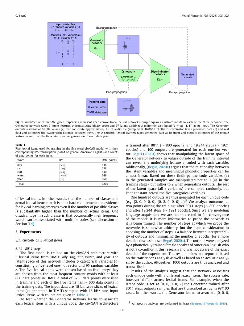

G. Beguš Neural Networks 139 (2021) 305–325

odf

TFco

5

Fig. 1. Architecture of fiwGAN: green trapezoids represent deep convolutional neural networks; purple squares illustrate inputs to each of the three networks. TheGenerator network takes 3 latent features φ (constituting binary code) and 97 latent variables z uniformly distributed (z ∼ U(−1, 1)) as its input. The Generatorutputs a vector of 16,384 values (x̂) that constitute approximately 1 s of audio file (sampled at 16,000 Hz). The Discriminator takes generated data (x̂) and realata and estimates the Wasserstein distance between them. The Q-network (lexical learner) takes generated data as its input and outputs estimates of the uniqueeature values that the Generator uses for generation of each data point.

able 1ive lexical items used for training in the five-word ciwGAN model with theirorresponding IPA transcription (based on general American English) and countsf data points for each item.Word IPA Data points

oily ["OIli] 638rag ["ôæg] 638suit ["sut] 630water ["wORÄ] 649year ["jIô] 650

Total 3205

of lexical items. In other words, that the number of classes andactual lexical items match is not a hard requirement and evidencefor lexical learning emerges even if the number of possible classesis substantially higher than the number of actual items. Onedisadvantage in such a case is that occasionally high frequencywords can be associated with multiple codes (see discussion inSection 3.4).

3. Experiments

3.1. ciwGAN on 5 lexical items

3.1.1. 8011 stepsThe first model is trained on the ciwGAN architecture withlexical items from TIMIT: oily, rag, suit, water, and year. The

latent space of this network includes 5 categorical variables (c)constituting a five-level one-hot vector and 95 random variablesz. The five lexical items were chosen based on frequency: theyare chosen from the most frequent content words with at least600 data points in TIMIT. A total of 3205 data points were usedin training and each of the five items has > 600 data points inthe training data. The input data are 16-bit .wav slices of lexicalitems (as annotated in TIMIT) sampled with 16 kHz rate. Inputlexical items with counts are given in Table 1.

To test whether the Generator network learns to associateeach lexical item with a unique code, the ciwGAN architecture

310

is trained after 8011 (∼ 800 epochs) and 19,244 steps (∼ 1921epochs) and 100 outputs are generated for each one-hot vec-tor. Beguš (2020a) shows that manipulating the latent space ofthe Generator network to values outside of the training intervalcan reveal the underlying feature encoded with each variable.Additionally, (Beguš, 2020a) argues that the relationship betweenthe latent variables and meaningful phonetic properties can bealmost linear. Based on these findings, the code variables (c)in the generated samples are manipulated not to 1 (as in thetraining stage), but rather to 2 when generating outputs. The restof the latent space (all z-variables) are sampled randomly, butkept constant across the five categorical variables.

One hundred outputs are thus generated for each unique code(e.g. [2, 0, 0, 0, 0], [0, 2, 0, 0, 0] ...).5 We analyze outcomes attwo points during the training: after 8011 steps (∼ 800 epochs)and after 19,244 steps (∼ 1921 epochs). Since we are modelinglanguage acquisition, we are not interested in full convergenceof the model: it is more informative to probe the network asit is being trained. The number of steps at which we probe thenetworks is somewhat arbitrary, but the main consideration inchoosing the number of steps is a balance between interpretabil-ity of outputs and minimizing the number of epochs (for a moredetailed discussion, see Beguš, 2020a). The outputs were analyzedby a phonetically trained female speaker of American English whois not a co-author in this research and was not aware of the exactdetails of the experiment. The results below are reported basedon the transcriber’s analysis as well as based on an acoustic analy-sis by the author. Altogether, 1000 outputs are thus analyzed andtranscribed.

Results of the analysis suggest that the network associateseach unique code with a different lexical item. The success rate,however, differs across lexical items. For example, when thelatent code is set at [0, 0, 0, 0, 2] the Generator trained after8011 steps outputs samples that are transcribed as rag in 98/100cases. In other words, the Generator learns to associate [0, 0, 0,

5 All acoustic analyses are performed in Praat (Boersma & Weenink, 2015).

G. Beguš Neural Networks 139 (2021) 305–325

0

urtbOttftaoofoth0a[a

fhsatobtnnt

fnsiptiitotha

tpn

f

wO

er

sgiu

pb

, 2] with rag.6 The Generator thus not only learns to generatespeech-like outputs, it also represents distinct lexical items witha unique representation: information that can be retrieved fromits outputs by the lexical learning network. We can argue that [0,0, 0, 0, 2] is the underlying representation of rag.7

To determine the underlying code for each lexical item, wese success rates (or estimates from the multinomial logisticegression model in Table 2 and Fig. 4): the lexical item that ishe most frequent output for a given latent code is assumed toe associated with that latent code (e.g. rag with [0, 0, 0, 0, 2]).ccasionally, a single lexical item is the most frequent output forwo latent codes. As will be shown below, it is likely the case thathis reflects imperfect learning where the underlying lexical itemor a latent code is obscured by a more frequent output (perhapshe one that is easier to distinguish from the data). In this case, wessociate such codes to the lexical item for which the given codeutputs the highest proportion of that lexical item with respect tother latent codes. For example, [0, 0, 0, 2, 0] outputs water mostrequently with oily accounting for approximately a quarter ofutputs. The assumed lexical item for [0, 0, 0, 2, 0] is oily, becausehe code that outputs water most frequently is [0, 0, 2, 0, 0], whileighest proportion of oily relative to other latent codes is for [0,, 0, 2, 0]. Observing the progress of lexical learning providesdditional evidence that oily is the underlying representation of0, 0, 0, 2, 0]: as the training progresses the network increasesccuracy (see Section 3.1.2).The success rate for the other four lexical items is lower than

or rag, but the outputs that deviate from the expected values areighly informative. For c = [2, 0, 0, 0, 0], the Generator (8011teps) outputs 72/100 data points that can be reliably transcribeds suit. In seven additional cases, the network outputs data pointshat can be transcribed with a sibilant [s] (79 total). In theseutputs, [s] is followed by a sequence that either cannot reliablye transcribed as suit or does not correspond to suit, but rathero year (transcribed as sear [sIô]). The remaining 21 outputs doot include the word for suit or a sibilant [s]. However, they areot randomly distributed across other four lexical items either —hey include lexical item year or its close approximation.8

An acoustic analysis of the training data reveals motivationsor the innovative deviating outputs. As already mentioned, theetwork occasionally generates an innovative output, sear. Theources of this innovation are likely four cases in the training datan which [j] in year ([jIô]) is realized as a post-alveolar fricative [S],robably due to contextual influence (something that could beranscribed as shear [SIô]). Fig. 2 illustrates all four examples. Thennovative generated output sear differs from the four examplesn the training data in one crucial aspect: the frication noise inhe generated output is that of a post-alveolar [s] rather than thatf a palato-alveolar [S]. Spectral analysis in Fig. 2 clearly showshat the center of gravity in the generated output is substantiallyigher than in the training data (which is characteristic of thelveolar fricative [s]).The innovative sear output likely results from the fact that

he training data contains four data points that pose a learningroblem: shear that features elements of suit and year. The in-ovative generated sear [sIô] consequently features (i) frication

noise that is approximately consistent with suit [sut] and (ii)ormant structure consistent with year [jIô]. It appears that thenetwork treats sear as a combination of the two lexical items.The network generates innovative outputs that combines the two

6 Occasionally, a short vocalic element precedes the ["ôæg].7 In the remaining two cases, the outputs include [ô] in the initial position,hich is followed by a diphthong [aI] and a period of a consonantal closure.ne output was transcribed as right.8 For raw counts in this and other models, see Tables A.5, A.6, A.7, and A.8.

311

elements (sear [sIô]). Additionally, the sear output seems to bequally distributed among the two latent codes, [2, 0, 0, 0, 0]epresenting suit and [0, 2, 0, 0, 0] representing year. In otherwords, the error rate distribution of the two latent codes suggeststhat the network classifies the output sear as the combination ofelements consistent with [2, 0, 0, 0, 0] and [0, 2, 0, 0, 0].

For c = [0, 2, 0, 0, 0], the Generator outputs 68 data pointsthat can be reliably transcribed as year or at least have a clear[Iô] sequence (without an [s]).9 22 outputs feature a sibilant [s].In these 22 cases, 16 can reliably be transcribed as suit, while theothers are mostly variants of the innovative sear. The remainingcases (approximately 10) are difficult to categorize based onacoustic analysis.

For [0, 0, 2, 0, 0], the Generator outputs 84 data points thatare transcribed as containing water [wORÄ]. In approximately 15of the 84 cases, the output involves an innovative combinationtranscribed as watery ["wOR@ôi]. Fig. 3 illustrates one such case.Watery is an innovative output that combines segment [i] fromoily (["OIli]) with ["wOR@ô] from water into a linguistically inter-pretable innovation. This suggests that the Generator outputs anovel combination of segments, based on analogy to oily. Unlikefor sear, the training data contained no direct motivations basedon which watery could be formed.10

Finally, for [0, 0, 0, 2, 0], the Generator outputs only 26 outputsthat can reliably be transcribed as oily ["OIli]. On the other hand,61 outputs contain water. Oily is the less frequent output for [0,0, 0, 2, 0] compared to water, but water is assigned to [0, 0, 2, 0,0] because it is its most frequent output, while [0, 0, 0, 2, 0] is thecode that outputs the highest proportion of oily. This is why weanalyze oily as the underlying lexical item for the [0, 0, 0, 2, 0]code. Another evidence that oily might underly the [0, 0, 0, 2, 0]code is that as the training progresses, the Generator increasesthe number of outputs transcribed with oily for this code anddecreases the number of outputs water for the same code (seeSection 3.1.2 and Fig. 4). For a confirmation that the proposedmethod for assigning underlying assumed words for a given codebased on annotated outputs yields valid results, see Section 3.3.2.

To evaluate lexical learning in the ciwGAN model statistically,we analyze the results with a multinomial logistic regressionmodel. To test significance of the latent code as the predictor ofthe lexical item, annotations of the generated data were codedand fit to a multinomial logistic regression model using the nnetpackage (Venables & Ripley, 2002) in R Core Team (2018). Thedependent variable is the transcriptions of the generated outputsfor the five lexical items and the else condition.11 The inde-pendent variable is a single predictor: the latent code with thefive levels that correspond to the five unique one-hot values inthe latent code. The difference in AIC between the model withthe latent code as a predictor (AIC = 674.7) vs. the emptymodel (AIC = 1707.1) suggests that the latent code is indeed aignificant predictor of the lexical item in the output. Counts areiven in Table 2. Estimates from the multinomial logistic modeln Fig. 4 clearly show that each lexical item is associated with anique latent code.

9 The initial consonant is sometimes absent from transcriptions, but this isrimarily because the glide interval is acoustically not prominent, especiallyefore [I].10 In 10 further cases of [0, 0, 2, 0, 0], the Generator outputs data points thatcontain a sequence oil ["OIl]. Transcription of the remaining 6 outputs is uncertain.11 The following conditions were used for coding the transcribed output: if theannotator transcribed an output as containing ‘‘suit’’, the coded lexical item wassuit), if ‘‘ear’’ or ‘‘eer’’ (and no ‘‘s’’ immediately preceding), then year, if involving‘‘water’’, ‘‘oil’’, and ‘‘rag’’, then water, oily, rag, respectively. In all other cases,the output was coded as else.

G. Beguš Neural Networks 139 (2021) 305–325

Fig. 2. Waveforms (top), spectrograms (mid, from 0–8000 Hz), and 25 ms spectra (slices indicated in the spectrograms) (bottom) of four data points of the lexicalitem year with clear frication noise in the training data (from TIMIT) and the generated innovative output sear.

Fig. 3. A waveform and spectrogram (0–4000 Hz) of an innovative output watery ["wOR@ôi] (top right). That innovative watery is a combination of water ["wORÄ] andoily ["OIli] is illustrated by two examples from the training data (top and bottom right). The innovative output watery features a clear formant structure of water witha high front vowel [i], characteristic of the lexical item oily (see marked areas of the spectrograms). At 19,244 steps, the vocalic structure of [i] is not present in theoutput, given the exact same latent code and random latent space. The network thus corrects the formant structure from an innovative watery into water ["wOR@ô(@)]as the training progresses. In some other cases, the network at 19,244 steps outputs oily for what was watery at 8011 steps.

Table 2Generated outputs and their percentages across the five one-hot vectors in the latent code. Transcriptions of theoutputs were coded as detailed in footnote 11.Assumed word Latent code c Most frequent % 2nd most freq. % Else

suit [2, 0, 0, 0, 0] suit ["sut] 72% year ["jIô] 21% 7%year [0, 2, 0, 0, 0] year ["jIô] 70% suit ["sut] 12% 18%water [0, 0, 2, 0, 0] water ["wORÄ] 84% oily ["OIli] 10% 6%oily [0, 0, 0, 2, 0] water ["wORÄ] 61% oily ["OIli] 26% 13%rag [0, 0, 0, 0, 2] rag ["ôæg] 98% – – 2%

312

G. Beguš Neural Networks 139 (2021) 305–325

mat

3

tltiwew

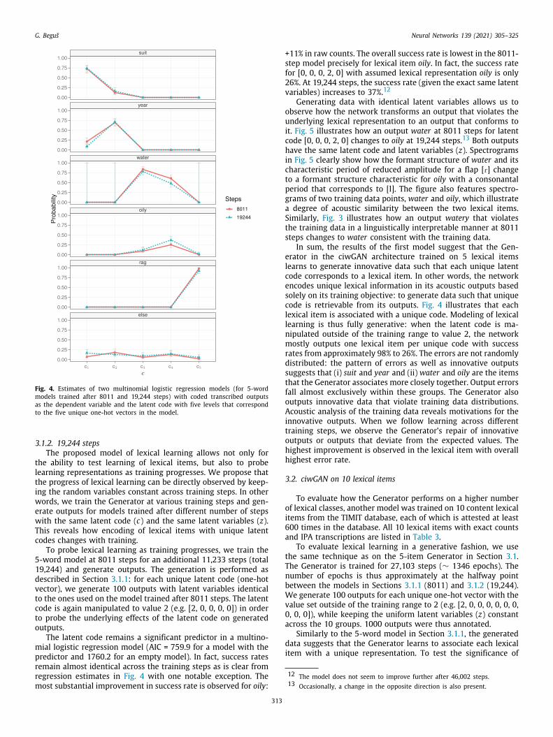
Fig. 4. Estimates of two multinomial logistic regression models (for 5-wordodels trained after 8011 and 19,244 steps) with coded transcribed outputss the dependent variable and the latent code with five levels that correspondo the five unique one-hot vectors in the model.

.1.2. 19,244 stepsThe proposed model of lexical learning allows not only for

he ability to test learning of lexical items, but also to probeearning representations as training progresses. We propose thathe progress of lexical learning can be directly observed by keep-ng the random variables constant across training steps. In otherords, we train the Generator at various training steps and gen-rate outputs for models trained after different number of stepsith the same latent code (c) and the same latent variables (z).

This reveals how encoding of lexical items with unique latentcodes changes with training.

To probe lexical learning as training progresses, we train the5-word model at 8011 steps for an additional 11,233 steps (total19,244) and generate outputs. The generation is performed asdescribed in Section 3.1.1: for each unique latent code (one-hotvector), we generate 100 outputs with latent variables identicalto the ones used on the model trained after 8011 steps. The latentcode is again manipulated to value 2 (e.g. [2, 0, 0, 0, 0]) in orderto probe the underlying effects of the latent code on generatedoutputs.

The latent code remains a significant predictor in a multino-mial logistic regression model (AIC = 759.9 for a model with thepredictor and 1760.2 for an empty model). In fact, success ratesremain almost identical across the training steps as is clear fromregression estimates in Fig. 4 with one notable exception. Themost substantial improvement in success rate is observed for oily:

313

+11% in raw counts. The overall success rate is lowest in the 8011-step model precisely for lexical item oily. In fact, the success ratefor [0, 0, 0, 2, 0] with assumed lexical representation oily is only26%. At 19,244 steps, the success rate (given the exact same latentvariables) increases to 37%.12

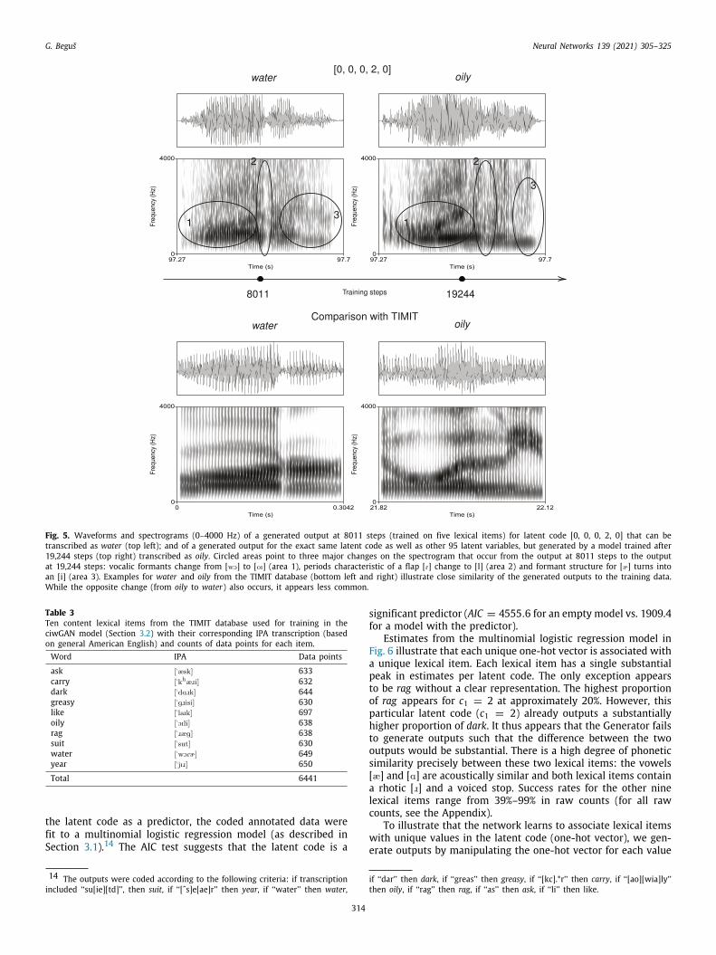
Generating data with identical latent variables allows us toobserve how the network transforms an output that violates theunderlying lexical representation to an output that conforms toit. Fig. 5 illustrates how an output water at 8011 steps for latentcode [0, 0, 0, 2, 0] changes to oily at 19,244 steps.13 Both outputshave the same latent code and latent variables (z). Spectrogramsin Fig. 5 clearly show how the formant structure of water and itscharacteristic period of reduced amplitude for a flap [R] changeto a formant structure characteristic for oily with a consonantalperiod that corresponds to [l]. The figure also features spectro-grams of two training data points, water and oily, which illustratea degree of acoustic similarity between the two lexical items.Similarly, Fig. 3 illustrates how an output watery that violatesthe training data in a linguistically interpretable manner at 8011steps changes to water consistent with the training data.

In sum, the results of the first model suggest that the Gen-erator in the ciwGAN architecture trained on 5 lexical itemslearns to generate innovative data such that each unique latentcode corresponds to a lexical item. In other words, the networkencodes unique lexical information in its acoustic outputs basedsolely on its training objective: to generate data such that uniquecode is retrievable from its outputs. Fig. 4 illustrates that eachlexical item is associated with a unique code. Modeling of lexicallearning is thus fully generative: when the latent code is ma-nipulated outside of the training range to value 2, the networkmostly outputs one lexical item per unique code with successrates from approximately 98% to 26%. The errors are not randomlydistributed: the pattern of errors as well as innovative outputssuggests that (i) suit and year and (ii) water and oily are the itemsthat the Generator associates more closely together. Output errorsfall almost exclusively within these groups. The Generator alsooutputs innovative data that violate training data distributions.Acoustic analysis of the training data reveals motivations for theinnovative outputs. When we follow learning across differenttraining steps, we observe the Generator’s repair of innovativeoutputs or outputs that deviate from the expected values. Thehighest improvement is observed in the lexical item with overallhighest error rate.

3.2. ciwGAN on 10 lexical items

To evaluate how the Generator performs on a higher numberof lexical classes, another model was trained on 10 content lexicalitems from the TIMIT database, each of which is attested at least600 times in the database. All 10 lexical items with exact countsand IPA transcriptions are listed in Table 3.

To evaluate lexical learning in a generative fashion, we usethe same technique as on the 5-item Generator in Section 3.1.The Generator is trained for 27,103 steps (∼ 1346 epochs). Thenumber of epochs is thus approximately at the halfway pointbetween the models in Sections 3.1.1 (8011) and 3.1.2 (19,244).We generate 100 outputs for each unique one-hot vector with thevalue set outside of the training range to 2 (e.g. [2, 0, 0, 0, 0, 0, 0,0, 0, 0]), while keeping the uniform latent variables (z) constantacross the 10 groups. 1000 outputs were thus annotated.

Similarly to the 5-word model in Section 3.1.1, the generateddata suggests that the Generator learns to associate each lexicalitem with a unique representation. To test the significance of

12 The model does not seem to improve further after 46,002 steps.13 Occasionally, a change in the opposite direction is also present.

G. Beguš Neural Networks 139 (2021) 305–325

aW

TTco

i

Fig. 5. Waveforms and spectrograms (0–4000 Hz) of a generated output at 8011 steps (trained on five lexical items) for latent code [0, 0, 0, 2, 0] that can betranscribed as water (top left); and of a generated output for the exact same latent code as well as other 95 latent variables, but generated by a model trained after19,244 steps (top right) transcribed as oily. Circled areas point to three major changes on the spectrogram that occur from the output at 8011 steps to the outputat 19,244 steps: vocalic formants change from [wO] to [oI] (area 1), periods characteristic of a flap [R] change to [l] (area 2) and formant structure for [Ä] turns inton [i] (area 3). Examples for water and oily from the TIMIT database (bottom left and right) illustrate close similarity of the generated outputs to the training data.hile the opposite change (from oily to water) also occurs, it appears less common.

able 3en content lexical items from the TIMIT database used for training in theiwGAN model (Section 3.2) with their corresponding IPA transcription (basedn general American English) and counts of data points for each item.Word IPA Data points

ask ["æsk] 633carry ["khæôi] 632dark ["dAôk] 644greasy ["gôisi] 630like ["laIk] 697oily ["OIli] 638rag ["ôæg] 638suit ["sut] 630water ["wORÄ] 649year ["jIô] 650

Total 6441

the latent code as a predictor, the coded annotated data werefit to a multinomial logistic regression model (as described inSection 3.1).14 The AIC test suggests that the latent code is a

14 The outputs were coded according to the following criteria: if transcriptionncluded ‘‘su[ie][td]’’, then suit, if ‘‘[ˆs]e[ae]r’’ then year, if ‘‘water’’ then water,

t

314

significant predictor (AIC = 4555.6 for an empty model vs. 1909.4for a model with the predictor).

Estimates from the multinomial logistic regression model inFig. 6 illustrate that each unique one-hot vector is associated witha unique lexical item. Each lexical item has a single substantialpeak in estimates per latent code. The only exception appearsto be rag without a clear representation. The highest proportionof rag appears for c1 = 2 at approximately 20%. However, thisparticular latent code (c1 = 2) already outputs a substantiallyhigher proportion of dark. It thus appears that the Generator failsto generate outputs such that the difference between the twooutputs would be substantial. There is a high degree of phoneticsimilarity precisely between these two lexical items: the vowels[æ] and [A] are acoustically similar and both lexical items containa rhotic [ô] and a voiced stop. Success rates for the other ninelexical items range from 39%–99% in raw counts (for all rawcounts, see the Appendix).

To illustrate that the network learns to associate lexical itemswith unique values in the latent code (one-hot vector), we gen-erate outputs by manipulating the one-hot vector for each value

if ‘‘dar’’ then dark, if ‘‘greas’’ then greasy, if ‘‘[kc].*r’’ then carry, if ‘‘[ao][wia]ly’’hen oily, if ‘‘rag’’ then rag, if ‘‘as’’ then ask, if ‘‘li’’ then like.

G. Beguš Neural Networks 139 (2021) 305–325

alvNc

Fig. 6. Estimates of a multinomial logistic regression model with coded tran-scribed outputs as the dependent variable and the latent code with ten levelsthat correspond to the ten unique one-hot vectors in the model trained on tenlexical items from TIMIT after 27,103 steps.

and by keeping the rest of the latent space (z) constant. Suchmanipulation can result in generated samples, where each

atent space outputs a distinct lexical item associated with thatalue ([20000000000] outputs dark, [02000000000]water, etc.).15ote that the acoustic contents of the generated outputs thatorrespond to each lexical item are substantially different (as

15 Often each series outputs one or two divergences from the ideal output.

p

315

Table 4Eight content lexical items from the TIMIT database used for training in thefiwGAN architecture (Section 3.3) with their corresponding IPA transcription(based on general American English) and counts of data points for each item.Word IPA Data points

ask ["æsk] 633carry ["khæôi] 632dark ["dAôk] 644greasy ["gôisi] 630like ["laIk] 697suit ["sut] 630water ["wORÄ] 649year ["jIô] 650

Total 5165

illustrated by the spectrograms in Fig. 7), which means that thelatent code (c) needs to be strongly associated with the individuallexical items, given that all the other 90 variables in the latentspace (the z-variables which constitute 90% of all latent space)are kept constant and that the entire change of the output occursonly due to change of the latent code c. In other words, by onlychanging the latent code and setting the variables to desiredvalues while keeping the rest of the latent space constant, we cangenerate desired lexical items with the Generator network.

3.3. fiwGAN on 8 lexical items

To evaluate lexical learning in a fiwGAN architecture, we trainthe fiwGAN model with three featural variables (φ). Because thelatent code in fiwGAN is binomially distributed, three featuralvariables correspond to 23

= 8 categories. The model was trainedon 8 content lexical items with more than 600 attestations in theTIMIT database (listed in Table 4). The model used for the analysiswas trained after 20,026 steps which correspond to a similarnumber of epochs as the 10-word ciwGAN model in Section 3.2(∼ 1241 epochs). Like for the ciwGAN models (Sections 3.1 and3.2), we generate 100 outputs for each unique binary code giventhe 3 featural variables with the values of the features set outsideof the training range to 2 instead of 1: [0, 0, 0], [0, 0, 2], [0, 2, 0],[0, 2, 2], [2, 0, 0], etc.

As expected, learning in the fiwGAN architecture is morechallenging compared to ciwGAN. The network has only log2(n)variables to encode n lexical items (compared to n variables forn classes in ciwGAN). Despite the latent space for lexical learningbeing highly reduced, an analysis of generated data in the fiwGANarchitecture suggests that the Generator learns to associate eachbinary code with a distinct lexical item (for an additional test, seeSection 3.3.2).

To test significance of the featural code (φ) as a predictor,the annotated data were fit to a multinomial logistic regressionmodel as in Sections 3.1 and 3.2. The dependent variables areagain coded transcriptions16 and the independent variable is thefeatural code (φ) with the eight unique levels as predictors: eachfor unique binary code. The difference in AIC between the modelthat includes the unique featural codes as predictors (φ) and theempty model (2038.5 vs. 3409.7) suggests that featural values aresignificant predictors.

Estimates of the regression model in Fig. 8 illustrate that mostlexical items receive a unique featural representation. Six out ofeight lexical items (dark, ask, suit, greasy, year and carry) all havedistinct latent featural representations that can be associatedwith these lexical items. Success rates for the six items have a

16 The outputs are coded as described in fn. 14 for the 10-word ciwGANmodel, except that if ‘‘[ae].*[sf]’’, then ask, because outputs contain a largeroportion of s-like frication noise that can also be transcribed with f.

G. Beguš Neural Networks 139 (2021) 305–325

l

pfdeib

cnlws

ma

Fig. 7. Waveforms and spectrograms (0–8000 Hz) of generated outputs (of a model trained on 10 items after 27,103 steps) when only the latent code is manipulatedand the remaining 90 latent random variables are kept constant across all 10 outputs. Transcriptions (by the author) suggest that each lexical item is associatedwith a unique representation.

gWt

8cvoTw2tm

toieTGo

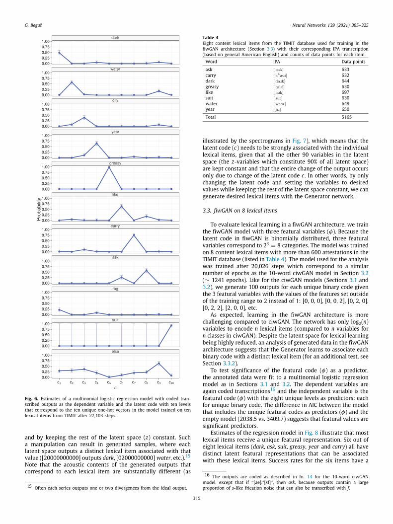
tatif2[gn[afaauT(oc

mean of 50.8% (in raw counts) with the range of 46% to 61%.Crucially, there appears to be a single peak in regression estimatesper lexical item for these six words, although the peaks are lessprominent compared to the ciwGAN architecture (expectedly so,since learning is significantly more challenging in the featuralcondition). Water and like are more problematic: [0, 2, 0] outputsike and water at approximately the same rate. It is possiblethat learning of the two lexical items is unsuccessful. Anotherpossibility is that [0, 2, 0] is the underlying representation ofwater because it is water ’s most frequent code that is not alreadytaken by another lexical item. According to the guidelines in Sec-tion 3.1, like would have to be represented by [0, 0, 0], because itoutputs the highest proportion of like that is not already taken foranother lexical items. That this assignment of underlying valuesof each featural representation is valid is additionally suggestedby another test in Section 3.3.2.

In the fiwGAN architecture, we can also test significance ofeach of the three unique features (φ1, φ2, and φ3). The annotateddata were fit to the same multinomial logistic regression modelas above, but with three independent variables: the three featureseach with two levels (0 and 2). AIC is lowest when all threevariables are present in the model (2135.5) compared to whenφ1, φ2, or φ3 are removed from the model (2527.2, 2413.0, and2773.3, respectively).

3.3.1. Featural learningAn advantage of the fiwGAN architecture is that it can model

classification (i.e. lexical learning) and featural learning of pho-netic and phonological representations simultaneously. We canassume that lexical learning is represented by the unique binarycode for each lexical item. Phonetic and phonological informationcan be simultaneously encoded with each unique feature (φ). Thathonetic and phonological information is learned with binaryeatures has been the prevalent assumption in linguistics forecades (Clements, 1985; Hayes, 2009). Recently, neuroimagingvidence suggesting that phonetic and phonological informations stored as signals that approximate phonological features haseen presented in Mesgarani et al. (2014).An analysis of featural learning in fiwGAN — how featural

odes simultaneously represent unique lexical items and pho-etic/phonological representations, can be performed by usingogistic regression as proposed in the following paragraphs asell as with a number of exploratory techniques described in thisection.Three out of eight lexical items used in training of the fiwGAN

odel include the segment [s]: a voiceless alveolar fricative withdistinct phonetic marker — a period of frication noise. The

316

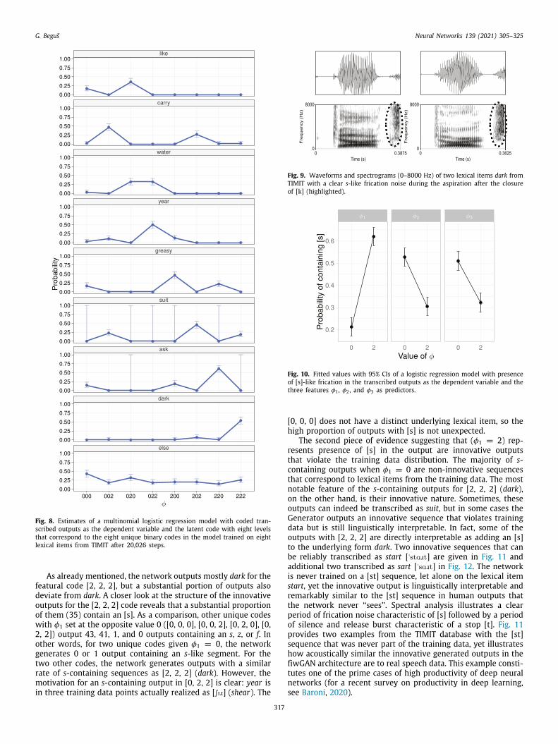
assumed binary codes for the three items containing [s], ask,reasy, and suit are [2, 2, 0], [2, 0, 0], and [2, 0, 2] (see Fig. 8).e observe that value 2 for feature φ1 is common to all three of

he lexical items containing an [s].To test the effects of φ1 on presence of [s] in the output,

00 annotated outputs (100 for each of the eight unique binaryodes) were fit to a logistic regression model. The dependentariable is presence of a s-like frication noise: if a transcribedutput contains an s, z, or f, the output is coded as success.he independent predictors in the model are the three featuresithout interactions: φ1, φ2, and φ3, each with two levels (0 and). Fig. 10 features estimates of the regression model. While allhree features are significant predictors, the effect appears to beost prominent for φ1.It is possible that the Generator network in the fiwGAN archi-

ecture uses feature φ1 to encode presence of segment [s] in theutput. This distribution can also be due to chance. Further works needed to test whether presence of phonetic/phonological el-ments in the output can be encoded with individual features.wo facts from the generated data, however, suggest that theenerator in the fiwGAN architecture associates φ1 with presencef [s].First, while ask, greasy, and suit all have φ1 = 2 in common,

he fourth unique featural code with φ1 = 2 ([2, 2, 2]) isssociated with dark. Spectral analysis of lexical item dark in theraining data reveals that aspiration of [k] in dark is in the train-ng data from TIMIT frequently realized precisely as an alveolarricative [s] (likely due to contextual influences).17 Approximately7% data points for dark in the training data from TIMIT contain as]-like frication noise during the aspiration period of [k].18 Fig. 9ives two such examples from TIMIT of dark with a clear fricationoise characteristic of an [s] sound after the aspiration noise ofk]. In other words, 3 lexical items in the training data containn [s] as part of their phonemic representation and thereforeeature it consistently. The Generator outputs data such thatsingle feature (φ1 = 2) is common to all three items. An

dditional item often involves a s-like element and the networkses the same value (φ1 = 2) for its unique code ([2, 2, 2]).here is approximately a 8.6% chance this distribution is randomof 70 possible featural code assignment for eight items, fourf which contain some phonetic feature such as [s], six or 8.6%ombinations contain the same value in one feature).

17 In many TIMIT sentences, dark appears before suit which causes theaspiration of [k] to be influenced by the following [s].18 This estimate is based on acoustic analysis of the first 100 training datapoints from the TIMIT database.

G. Beguš Neural Networks 139 (2021) 305–325

fdoow2ogtrmi

rt

Fig. 8. Estimates of a multinomial logistic regression model with coded tran-scribed outputs as the dependent variable and the latent code with eight levelsthat correspond to the eight unique binary codes in the model trained on eightlexical items from TIMIT after 20,026 steps.

As already mentioned, the network outputs mostly dark for theeatural code [2, 2, 2], but a substantial portion of outputs alsoeviate from dark. A closer look at the structure of the innovativeutputs for the [2, 2, 2] code reveals that a substantial proportionf them (35) contain an [s]. As a comparison, other unique codesith φ1 set at the opposite value 0 ([0, 0, 0], [0, 0, 2], [0, 2, 0], [0,, 2]) output 43, 41, 1, and 0 outputs containing an s, z, or f. Inther words, for two unique codes given φ1 = 0, the networkenerates 0 or 1 output containing an s-like segment. For thewo other codes, the network generates outputs with a similarate of s-containing sequences as [2, 2, 2] (dark). However, theotivation for an s-containing output in [0, 2, 2] is clear: year is

n three training data points actually realized as [SIô] (shear). The

317

Fig. 9. Waveforms and spectrograms (0–8000 Hz) of two lexical items dark fromTIMIT with a clear s-like frication noise during the aspiration after the closureof [k] (highlighted).

Fig. 10. Fitted values with 95% CIs of a logistic regression model with presenceof [s]-like frication in the transcribed outputs as the dependent variable and thethree features φ1 , φ2 , and φ3 as predictors.

[0, 0, 0] does not have a distinct underlying lexical item, so thehigh proportion of outputs with [s] is not unexpected.

The second piece of evidence suggesting that (φ1 = 2) rep-esents presence of [s] in the output are innovative outputshat violate the training data distribution. The majority of s-containing outputs when φ1 = 0 are non-innovative sequencesthat correspond to lexical items from the training data. The mostnotable feature of the s-containing outputs for [2, 2, 2] (dark),on the other hand, is their innovative nature. Sometimes, theseoutputs can indeed be transcribed as suit, but in some cases theGenerator outputs an innovative sequence that violates trainingdata but is still linguistically interpretable. In fact, some of theoutputs with [2, 2, 2] are directly interpretable as adding an [s]to the underlying form dark. Two innovative sequences that canbe reliably transcribed as start ["stAôt] are given in Fig. 11 andadditional two transcribed as sart ["sAôt] in Fig. 12. The networkis never trained on a [st] sequence, let alone on the lexical itemstart, yet the innovative output is linguistically interpretable andremarkably similar to the [st] sequence in human outputs thatthe network never ‘‘sees’’. Spectral analysis illustrates a clearperiod of frication noise characteristic of [s] followed by a periodof silence and release burst characteristic of a stop [t]. Fig. 11provides two examples from the TIMIT database with the [st]sequence that was never part of the training data, yet illustrateshow acoustically similar the innovative generated outputs in thefiwGAN architecture are to real speech data. This example consti-tutes one of the prime cases of high productivity of deep neuralnetworks (for a recent survey on productivity in deep learning,see Baroni, 2020).

G. Beguš Neural Networks 139 (2021) 305–325

sts

f

3

cyan

Fig. 11. (left) Waveforms and spectrograms (0–8000 Hz) of two innovative outputs for φ = [2, 2, 2] transcribed as ["stAôt]. The fiwGAN network trained after 20,026teps thus outputs innovative sequence [st] that is absent from the training data, but is a linguistically interpretable output that can be interpreted as adding [s]o dark. (right) Waveforms and spectrograms (0–8000 Hz) of two lexical items from TIMIT that are not part of training data, but illustrate that the innovative [st]equence in the generated data is acoustically very similar to the [st] sequence in human outputs that the network has no access to.

v0t8ac

Fig. 12. Waveforms and spectrograms (0–8000 Hz) of two innovative outputsor φ = [2, 2, 2] transcribed as ["sAôt].

.3.2. Underlying representationsBeguš (2020a) argues that the underlying value of a feature

an be uncovered by manipulating a given feature well be-ond the training range. For example, Beguš (2020a) proposestechnique for identifying variables that correspond to pho-etic/phonological properties in the outputs. By setting the values

318

of the identified features well beyond the training range, thenetwork almost exclusively outputs the desired property (e.g. asegment [s] in the output).

This effect of the underlying value of a variable is even moreprominent in the fiwGAN architecture. When the values of latentfeatures (φ) are set at 0 and 2, success rates appear at approxi-mately 50% (Fig. 8). Value 2 was chosen for analysis in Section 3.3,because non-categorical outcomes yield more insights into learn-ing. However, we can reach almost categorical accuracy whenthe values are set substantially higher than 2. For example, whenwe generate outputs with values of featural code set at 5 ([5, 5,5]), the network generates 93/100 outputs19 that can be reliablytranscribed as dark and another 7 that closely resemble dark, buthave a period of frication instead of the initial stop (sark). Witheven higher values such as 15, the Generator outputs 100/100samples transcribed as dark for [15, 15, 15]. Similarly, [5, 5, 0]yields ask in 97/100 cases; it yields an innovative output withfinal [i] in three cases. At [15, 15, 0], the Generator outputs100/100 ask. The success rates differ across featural codes, butalue 15 triggers almost categorical outputs for most of them. [15,, 0] yields 93/100 greasy (1 unclear and 6 ask). For [15, 0, 15],he network outputs a [sVt] sequence for suit (where V=vowel)7/100 times. In 13 examples, the frication noise does not havepronounced s-like frication noise, but is more distributed andloser to aspiration noise of [k]. The identity of the vowel is

19 Counts in this sections are performed by the author only.

G. Beguš Neural Networks 139 (2021) 305–325

isFvr

oiyo[(

ltltuaWbabFn

cvdptulocr

iitug

3

lefi6cniwow

Tha

w

s

ontatoteFasvl

ntriguing: the formant values are not characteristic of [u] (as inuit), but rather of a lower more central vowel (F1 = 663 Hz,2 = 1618 Hz, F3 = 2515 Hz for one listing). Since formantariability is high in the training data, the underlying prototypicalepresentation likely defaults to a more central vowel.

[0, 0, 15] yields carry in 100/100 outputs, but in 13 of theseutputs the aspiration noise of [k] is distributed with a peakn higher frequencies for an acoustic effect of [ts]. [0, 15, 0]ields 100/100 water. The acoustic output is reduced to includenly the main acoustic properties of water: formant structure forwO] followed by a consonantal period for [R] and a very briefsometimes missing) vocalic period (Fig. 13).

The only two codes that do not yield straightforward under-ying representations are [0, 0, 0] and [0, 2, 2]. It appears thathe Generator is unable to strongly associate [0, 0, 0] with anyexical representation, likely due to lack of positive values inhis particular code. This means that the network needs to learnnderlying representations for two remaining lexical items withsingle code: like and year, both likely associated with [0, 2, 2].hen set to [0, 5, 5], the Generator outputs both like and year,20ut at [0, 10, 10] and [0, 15, 15] the underlying representation isn acoustic output that is difficult to characterize and is likely alend of the two representations (acoustically closer to like; seeig. 13). Future analyses should thus include log2(n) variables for− 1 classes in the fiwGAN architecture.Another interesting fact emerges when we set the featural

odes to high values such as 5 or 15. The outputs at these highalues are minimally variable: the outputs are almost identicalespite the 97 random latent variables z being randomly sam-led for each output, as illustrated by Fig. 13. It appears thathe network associates unique featural codes with prototypicalnderlying representations of lexical items. When values areower, other random latent variables (z) cause variation in theutputs, but the high values (such as 5 or 15) of the featuralodes φ override this variation and reveal the underlying lexicalepresentation for each featural code.

The generative test with values set well above the train-ng range strongly suggests that the Generator associates lexicaltems with unique codes and likely represents them with proto-ypical acoustic values. The test also confirms that the assumednderlying lexical items identified with multinomial logistic re-ression (Fig. 8) are correct.

.4. fiwGAN on the entire TIMIT

To test how the proposed architecture scales to substantiallyarger training datasets, we train the fiwGAN architecture on thentire TIMIT database. TIMIT was sliced for words into the sameormat as described in Section 3.1.1, which yields 54,378 lexicaltems in the training data. Because TIMIT contains approximately,229 unique lexical items, we train the fiwGAN network with 13ode variables, which allows for 213

= 8,192 unique classes. Theumber of possible classes is higher than the number of uniquetems (by about 1,963 or 24.0%). This experiment thus also testshether lexical learning emerges in a model in which the numberf classes differs from the number of lexical items. The networkas trained for 179,528 steps (∼1056 epochs).21Training the networks to learn lexical items from the entire

IMIT is a challenging task. First, neither the Generator (testedere for lexical learning) nor the Q-network (forcing the Gener-tor to output informative data) have direct access to the data.

20 Occasionally, [0, 5, 5] also yields an output that can be characterized asater.21 The training on an NVIDIA GeForce GTX 1080 Ti takes approximately 160teps per 300 s for a total of ∼ 4 days and 12 h. The models with higher numberof steps face mode collapse issues, common in the GAN architecture.

319

The only network that actually has a direct access to the trainingdata is the Discriminator, which is the least relevant network inthe architecture for learning lexical information. This stands instark contrast with the autoencoder architecture, in which thenetwork that learns lexical representations in its latent spacehas a direct access to the data. Second, TIMIT is highly variableand contains lexical items that are phonetically highly reduced.Many items contain only one token per item, and in general, thetoken distribution of the lexical items varies substantially. Thedimension of the vector representing lexical items in our modelsis highly reduced: only 13 binary code variables (13% of the latentvariables) are available to the model to encode identity of 6,229unique items with 54,378 total tokens.

Based on inferential statistical tests in Sections 3.1, 3.2, and3.3, we argued that the models show clear evidence for lexicallearning. In a model with fewer codes, we can fit all annotationsto a multinomial logistic regression model and perform hypoth-esis testing for lexical learning. In a larger model with the entireTIMIT as the training data, it is challenging to manually analyzeoutputs of all 8,192 binary codes given the thirteen latent features(φ) in the model. Instead, we use the argument from the modelswith fewer variables and test lexical learning by generating datawith a subset of possible latent codes. Evidence for lexical learn-ing is evaluated in the following way: if the Generator outputsone lexical item more often than other lexical items for eachunique code, it is reasonable to assume (based on the results inSections 3.1, 3.2, and 3.3) that the particular lexical item is theunderlying learned representation of the corresponding uniquecode, as is confirmed by statistical tests in the models with fewervariables.

Despite the highly challenging learning task and the mismatchbetween the number of classes and the number of actual lexicalitems, the fiwGAN does appear to show evidence for lexical learn-ing even when trained on the entire TIMIT dataset. We choose70 out of possible 8,192 unique latent codes and generate sets ofoutputs, each for one of the 70 chosen codes. We only manipulatethe latent code (φ) across the 70 sets of outputs; all other 87/100variables z are identical across the sets of outputs. The values ofthe latent code are set to 0 or either 1.0 or a slightly higher valueof 1.1 (with no substantial differences in outputs observed among1.0 or 1.1). As will be argued below, the Generator performs wellon the lexical learning task even when the latent variables are notmanipulated to marginal levels outside of the training range.22

Based on exploration of the 70 unique latent codes, three typesf outcomes are observed: (i) the Generator outputs predomi-antly one clearly identifiable lexical item for a latent code; (ii)he Generator outputs predominantly one sequence of sounds forlatent code, but the actual underlying lexical item is difficult

o establish; and (iii) the Generator outputs unclear and variableutputs for a latent code.23 The first and desired outcome, wherehe Generator outputs almost exclusively one lexical item that isasily recognizable per one latent code, is the most frequent.24or approximately 29 codes (out of 70 tested or 41.4%), the Gener-tor outputs mostly one clearly recognizable lexical item. Fig. 14hows the first ten generated outputs for fifteen out of 29 latentariables for which a clear underlying lexical item can be estab-ished. As already mentioned, the other latent variables (z) areidentical in the ten outputs across the 15 sets. There is relatively

22 In fact, the Generator outputs unintelligible outputs when values are ma-nipulated substantially outside of the training range (which stands in oppositionto the models in Sections 3.1, 3.2, and 3.3).23 All outputs in the current section were analyzed and annotated by theauthor.24 In some cases, the underlying lexical item is not the most frequent, but theonly one that is identifiable.

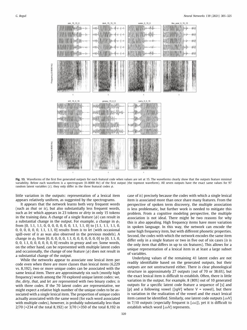
G. Beguš Neural Networks 139 (2021) 305–325

vr

la

(

iaf0sc

a

cvsft

Fig. 13. Waveforms of the first five generated outputs for each featural code when values are set at 15. The waveforms clearly show that the outputs feature minimalariability. Below each waveform is a spectrogram (0–8000 Hz) of the first output (the topmost waveform). All seven outputs have the exact same values for 97andom latent variables (z); they only differ in the three featural codes φ.

ipipatisSdtuo

rostvo[iiie

ittle variation in the outputs: representation of a lexical itemppears relatively uniform, as suggested by the spectrograms.It appears that the network learns both very frequent words

such as that or is), but also substantially less frequent words,such as let which appears in 23 tokens or dirty in only 15 tokensn the training data. A change of a single feature (φ) can result insubstantial change in the output. For example, a change in φ1

rom [0, 1.1, 1.1, 0, 0, 0, 0, 0, 0, 0, 1.1, 1.1, 0] to [1.1, 1.1, 1.1, 0,, 0, 0, 0, 0, 0, 1.1, 1.1, 0] results from is to let (with occasionalpill-over of is as was also observed in the previous models). Ahange in φ2 from [0, 0, 0, 0, 0, 1.1, 0, 0, 0, 0, 0, 0, 0] to [0, 1.1, 0,0, 0, 1.1, 0, 0, 0, 0, 0, 0, 0] results in greasy and see. Some words,on the other hand, can be represented with multiple latent codesand occasionally, the change of one feature (φ) does not result insubstantial change of the output.While the networks appear to associate one lexical item per

ode even when there are more classes than lexical items (6,229s. 8,192), two or more unique codes can be associated with theame lexical item. There are approximately six such (mostly highrequency) words among the 70 explored unique latent codes:we,he, dirty, that, and let are represented with two binary codes; iswith three codes. If the 70 latent codes are representative, wemight expect a relative high number of the unique codes to be as-sociated with a single lexical item. The proportion of unique codesactually associated with the same word (for each word associatedwith multiple codes), however, is probably substantially less than2/70 (=234 of the total 8,192) or 3/70 (=350 of the total 8,192 in

320

case of is) precisely because the codes with which a single lexicaltem is associated more than once share many features. From theerspective of spoken term discovery, the multiple associations less problematic, but further work is needed to mitigate thisroblem. From a cognitive modeling perspective, the multiplessociation is not ideal. There might be two reasons for whyhis is also appealing. High frequency items have more variationn spoken language. In this way, the network can encode theame high frequency item, but with different phonetic properties.econd, the codes with which the network encodes the same itemiffer only in a single feature or two in five out of six cases (is ishe only item that differs in up to six features). This allows for anique representation of a lexical item in at least a large subsetf variables.Underlying values of the remaining 41 latent codes are not

eadily identifiable based on the generated outputs, but theirutputs are not unstructured either. There is clear phonologicaltructure in approximately 27 outputs (out of 70 or 38.6%), buthe exact lexical item is difficult to establish. Often, there is littleariation in the output. For example, 8 (80%) out of 10 generatedutputs for a specific latent code feature a sequence of [s] andp] and a following vowel ([spV] where V = vowel), but theres variation in the realization of the vowel and the exact lexicaltem cannot be identified. Similarly, one latent code outputs [ôisV]n 7/10 outputs (especially frequent is [ôisi]), yet it is difficult tostablish which word [ôisV] represents.

G. Beguš Neural Networks 139 (2021) 305–325

v

nrorwia(tu

ee

Fig. 14. Waveforms and spectrograms of fifteen sets of outputs, each for one unique latent code value. Each set contains ten outputs in which the other 87 latentariables z are held constant across the fifteen sets. The Generator only outputs waveforms; spectrograms are given for the purpose of acoustic analysis.

to

t

There are two reasons for why the outputs in this group areot easily identifiable as lexical items. Either the networks doepresent unique lexical items with these codes, but the qualityf the audio output is not high enough for a lexical item to beecognizable, or the networks encode combinations of phonemesith latent codes rather than unique lexical items. In other words,

t is possible that sub-lexical units can be learned by the Gener-tor and used to encode information. In the remaining 14 cases20.0%), the network generates an unclear output that is difficulto identify as a lexical item and the outputs do not show aniform phonological structure either.Some evidence for complex sublexical featural learning

merges in the fiwGAN trained on the entire TIMIT too. Forxample, if φ5−7 are set to 1.1 and φ12 is set to 0, the Generator

frequently outputs a distinct initial velar stop [k] in six out of six

321

selected sets of outputs with this structure of the latent code.25[k]-initial words are not reliably identified at the beginning ofthe word in any of the other 64 tested codes. While the itemsexcept quite are not clear enough to fall in group (i), the initial[k] is clearly identifiable across the six sets. Apart from the initial[k], the outputs with this structure differ substantially in theirphonetic properties (e.g. outputs can approximate items such asculture, car(t), quite, color or [kV]). It is reasonable to assume thathe network encodes a sublexical phonetic property – presencef initial [k] – with a subset of latent features.The results suggest that the Generator at least partially learns

o encode lexical items with unique latent codes in the fiwGAN

25 There are more outputs with this structure of features that have not beentested.

G. Beguš Neural Networks 139 (2021) 305–325

aie4mltdltoai

4

enhttts

Gt2iditplifniiinia

GsdcofloceiotiWcchWtk

rchitecture even when trained on 54,378 tokens of 6,229 lexicaltems from TIMIT. Based on a subsample of latent codes, the Gen-rator outputs a clearly identifiable lexical item in approximately1.4% of tested codes. In most cases, the one lexical item is theajority output (as clear from Fig. 14) realized with relatively

ittle phonetic variability. There are many properties of TIMIT datahat the Generator could learn to encode into 8,192 classes, but itoes appear that it is precisely lexical items that the network isearning. This experiment also suggests that the Generator learnso represent lexical items with unique codes even if the numberf possible classes and the number of actual items do not matchnd even if there is a substantial difference in the frequency ofndividual items.

. Discussion and future directions

This paper proposes two architectures for unsupervised mod-ling of lexical learning from raw acoustic data with deep neuraletworks. The ability to retrieve information from acoustic data inuman speech is modeled with a Generator network that learnso output data that resemble speech and, simultaneously, learnso encode unique information in its outputs. We also proposeechniques for probing how deep neural networks trained onpeech data learn meaningful representations.The proposed fiwGAN and ciwGAN models are based on the

enerative Adversarial Network architecture and its implementa-ions in WaveGAN (Donahue et al., 2019), DCGAN (Radford et al.,015), and InfoGAN (Chen et al., 2016; Rodionov, 2018). Follow-ng Beguš (2020a), we model language acquisition as learning of aependency between the latent space and generated outputs. Wentroduce a network that forces the Generator to output data suchhat information is retrievable from its acoustic outputs and pro-ose a new structure of the latent variables that allows featuralearning and a very low-dimension vector representation of lex-cal items. Lexical learning emerges in an unsupervised mannerrom the architecture: the most efficient way for the Generatoretwork to output acoustic data such that unique informations retrievable from its data is to encode unique information ints acoustic outputs such that latent codes coincide with lexicaltems in the training data. The result is thus a deep convolutionaleural network that takes latent codes and variables and outputsnnovative data that resembles training data distributions as wells learns to associate lexical items with unique representations.Four experiments tested lexical learning in ciwGAN and fiw-

AN architectures trained on tokens of five, ten, eight, and 6,229liced lexical items in raw audio format from a highly variableatabase — TIMIT. The paper proposes that in smaller models lexi-al learning can be evaluated with multinomial logistic regressionn generated data. Evidence of lexical learning is present in allour experiments. It appears that the Generator learns to associateexical items with unique latent code — categorical (as in ciwGAN)r featural (as in fiwGAN). By manipulating the values of latentodes to value 2, the networks output unique lexical items forach unique code and reach accuracy that ranges from 98% to 26%n the five-word model. To replicate the results and test learningn a higher number of lexical items, the paper presents evidencehat the model learns to associate unique latent codes with lexicaltems in the 10-words model as well, with only one exception.hen trained on the entire TIMIT, the Generator outputs one

learly identifiable lexical item in approximately 41% of latentodes tested. The paper also proposes a technique for followingow the network learns representations as training progresses.e can directly observe how the network transforms an output

hat violates training data into an output that conforms to it byeeping the latent space constant as training progresses.

322

The fiwGAN architecture features, to our knowledge, a newproposal within the InfoGAN architecture: to model classifica-tion with featural codes instead of one-hot vectors. This shiftyields the potential to model featural learning and higher-levelclassification (i.e. phonetic/phonological features and unique lex-ical representations) simultaneously. The paper presents evidencesuggesting that the network might use some feature values toencode phonetic/phonological properties such as presence of [s].Regression models suggest that φ1 is associated with presenceof [s] in the output (and simple probabilistic calculation revealsabout 8.6% probability that the distribution is due to chance). Thestrongest evidence for simultaneous lexical and featural learningcomes from innovative outputs in the fiwGAN architecture. Thenetwork trained on lexical items that lack a sequence of a fricativeand a stop [st] altogether outputs an innovative sequence startor sart. These innovative outputs can be analyzed as adding asegment [s] (from suit) to dark, likely under the influence of thefact that φ1 represents presence of [s].

Innovative outputs that violate training data are informativefor both computational models of language acquisition as wellas for our understanding of what types of dependencies thenetworks are able to learn. We discuss several cases of innovativeoutputs. Some innovations are motivated by training data distri-butions (e.g. sear) and reveal how the networks treat acousticallysimilar lexical items. For other innovative outputs, such as watery,the training data contains no apparent motivations. We alsotrack changes from innovative to conforming outputs as trainingprogresses.

We argue that innovative outputs are linguistically inter-pretable and acoustically very similar to actual speech data thatis absent from the training data. For example, an innovative [st]sequence in start corresponds directly to human outputs withthis sequence that were never part of the training data. Furthercomparisons of this type should yield a better understanding onhow the combinatorial principle in human language can arisewithout language-specific parameters in a model.

The paper also discusses how internal representations in deepconvolutional networks can be identified and explored. We arguethat by setting the latent values substantially beyond the trainingrange (as suggested for phonological learning in Beguš, 2020a),the Generator almost exclusively outputs one unique lexical itemper each unique featural code (with only one exception) in thefiwGAN architecture on eight lexical items. In other words, forvery high values of the featural code (φ), lexical learning appearsto be near categorical. The variability of the outputs is minimalat such high values (e.g. 15). It appears that setting the featuralcode to such extreme values reveals the underlying representa-tion of each featural code. This property is highly desirable in amodel of language acquisition and has the potential to reveal theunderlying learned representations in the GAN architecture.

Several further experiments and improvements to the modelare left to future work. The proposed architecture allows testingof any property of the data and probing the learned representa-tion behind each latent code (or variable; as per Beguš, 2020a).For example, we can train the network on n latent codes orfeatures, which effectively means we are forcing the network tolearn n (or 2n) most informative categories in the data. Manipu-lating the latent codes to marginal levels represents a techniqueto test which properties about the data the network learns ina generative fashion. We can thus test how deep convolutionalnetworks learn informative properties about the data and directlyobserve what those categories are. Representation of any processin speech can thus be modeled (for an identity-based pattern,see Beguš, 2020b). Second, the current paper only analyzes theGenerator network in the generative fashion, but the architecturealso allows an analysis of the Q-network in discriminative lexical

G. Beguš Neural Networks 139 (2021) 305–325

TRa .

iu

A

A

able A.5aw counts for outcomes of the ciwGAN model trained on five lexical itemsfter 8011 steps (Section 3.1.1). The outcomes are coded as described in fn. 11

else rag oily water year suit

c1 7 0 0 0 21 72c2 18 0 0 0 70 12c3 6 0 10 84 0 0c4 13 0 26 61 0 0c5 2 98 0 0 0 0

Table A.6Raw counts for outcomes of the ciwGAN model trained on five items after 19,244steps (Section 3.1.2). The outcomes are coded as described in fn. 11.

else rag oily water year suit

c1 17 0 0 0 9 74c2 13 0 0 0 71 16c3 10 0 12 78 0 0c4 15 0 37 48 0 0c5 6 92 2 0 0 0

Table A.7Raw counts for outcomes of the ciwGAN model trained on ten items after 27,103steps (Section 3.2). The outcomes are coded as described in fn. 14.

else suit rag ask carry like greasy year oily water dark

c1 29 0 21 0 1 0 0 0 0 0 49c2 31 0 0 0 0 4 0 0 8 57 0c3 37 0 0 0 10 1 0 11 39 2 0c4 20 0 8 0 1 1 0 65 0 0 5c5 1 0 0 0 0 0 99 0 0 0 0c6 10 0 0 26 0 64 0 0 0 0 0c7 20 0 0 0 76 0 0 4 0 0 0c8 23 0 0 58 0 18 0 0 0 0 1c9 63 0 1 0 1 2 0 2 7 18 6c10 8 92 0 0 0 0 0 0 0 0 0

Table A.8Raw counts for outcomes of the fiwGAN model trained on eight items after20,026 steps (Section 3.3). The outcomes are coded as described in fn. 16.

else dark ask suit greasy year water carry like

[0, 0, 0] 43 0 15 0 17 3 3 2 17[0, 0, 2] 18 1 0 23 0 11 0 47 0[0, 2, 0] 32 0 0 0 0 0 32 0 36[0, 2, 2] 18 0 0 0 0 50 32 0 0[2, 0, 0] 20 1 19 0 47 13 0 0 0[2, 0, 2] 20 7 0 46 0 0 0 27 0[2, 2, 0] 15 1 61 0 22 0 0 1 0[2, 2, 2] 25 54 0 19 0 0 0 2 0

learning tasks (such as ABX). An experiment with novel unob-served test data fed to the Q-network would reveal the model’sability to assign unique codes to individual lexical items. Sucha network would be highly desirable in an unsupervised lexicallearning setting or for very low dimension acoustic word embed-ding tasks. Third, the paper proposes a technique to follow lexicallearning as training progresses (see Section 3.1). A superficialcomparison between lexical learning in the proposed models andlanguage-acquiring children could yield further insights into thecomputational modeling of language acquisition (for an overviewof the literature on how lexical learning progresses in languageacquisition, see Gaskell & Ellis, 2009). The proposed architecturecan also be used for testing lexical learning when trained onadult-directed vs. child-directed speech corpora. Finally, futuredirections should also include developing a model that couldparse lexical items from a continuous acoustic speech stream andimproving the model’s overall performance.

The proposed model of lexical learning has several furthermplications. Dependencies in speech data are significantly betternderstood than dependencies in visual data. A long scientific

323

tradition of studying dependencies in phonetic and phonologicaldata in human languages yields an opportunity to use linguisticdata to probe the types of dependencies deep neural networkscan or cannot learn (Beguš, 2020b). The proposed architecturesallow us to probe what types of dependencies the networks canlearn, how they encode unique information in the latent space,and how self-organization of retrievable information emerges inthe GAN architecture. The models also have some basic impli-cations for unsupervised text-to-speech generation tasks: ma-nipulating the latent variables to specific values results in theGenerator outputting desired lexical items.

Declaration of competing interest

The authors declare that they have no known competing finan-cial interests or personal relationships that could have appearedto influence the work reported in this paper.

Acknowledgments

This research was funded by a grant to new faculty at the Uni-versity of Washington and the University of California, Berkeley. Iwould like to thank Sameer Arshad for slicing data from the TIMITdatabase and Ella Deaton for annotating data.

Appendix. Raw counts

See Tables A.5–A.8.

References

Alishahi, A., Barking, M., & Chrupała, G. (2017). Encoding of phonology ina recurrent neural model of grounded speech. In Proceedings of the 21stconference on computational natural language learning (pp. 368–378). Van-couver, Canada: Association for Computational Linguistics, http://dx.doi.org/10.18653/v1/K17-1037, URL: https://www.aclweb.org/anthology/K17-1037.

rjovsky, M., Chintala, S., & Bottou, L. (2017). Wasserstein generative adver-sarial networks. In D. Precup, & Y. W. Teh (Eds.), Proceedings of the 34thinternational conference on machine learning (pp. 214–223). Sydney, Aus-tralia: International Convention Centre, URL: http://proceedings.mlr.press/v70/arjovsky17a.html.

rnold, D., Tomaschek, F., Sering, K., Lopez, F., & Baayen, R. H. (2017). Wordsfrom spontaneous conversational speech can be recognized with human-likeaccuracy by an error-driven learning algorithm that discriminates betweenmeanings straight from smart acoustic features, bypassing the phoneme asrecognition unit. PLoS One, 12, 1–16. http://dx.doi.org/10.1371/journal.pone.0174623.

Baayen, R. H., Chuang, Y. Y., Shafaei-Bajestan, E., & Blevins, J. P. (2019). Thediscriminative lexicon: A unified computational model for the lexicon andlexical processing in comprehension and production grounded not in (de)composition but in linear discriminative learning. Complexity, 2019, http://dx.doi.org/10.1155/2019/4895891.

Baevski, A., Schneider, S., & Auli, M. (2020). Vq-wav2vec: Self-supervisedlearning of discrete speech representations. In International conference onlearning representations (pp. 1–12). URL: https://openreview.net/forum?id=rylwJxrYDS.

Baroni, M. (2020). Linguistic generalization and compositionality in mod-ern artificial neural networks. Philosophical Transactions of the RoyalSociety, Series B (Biological Sciences), 375, Article 20190307. http://dx.doi.org/10.1098/rstb.2019.0307, URL: https://royalsocietypublishing.org/doi/abs/10.1098/rstb.2019.0307, arXiv:https://royalsocietypublishing.org/doi/pdf/10.1098/rstb.2019.0307.

Barry, S. M., & Kim, Y. E. (2019). Infowavegan: Informative latent spacesfor waveform generation. URL: http://nemisig2019.nemisig.org/images/kimSlides.pdf. poster at the North East Music Information Special InterestGroup.

Beguš, G. (2020a). Generative adversarial phonology: Modeling unsupervisedphonetic and phonological learning with neural networks. Frontiers in Artifi-cial Intelligence, http://dx.doi.org/10.3389/frai.2020.00044, URL: https://www.frontiersin.org/articles/10.3389/frai.2020.00044/abstract.

Beguš, G. (2020b). Identity-based patterns in deep convolutional networks:Generative adversarial phonology and reduplication. URL: https://arxiv.org/abs/2009.06110, arXiv:2009.06110.

G. Beguš Neural Networks 139 (2021) 305–325

B

B

B

C

C

C

C

G

G

H

H

H

H

K

K

K

K

L

L

L

M

N

P

R

R

R

oersma, P., & Weenink, D. (2015). Praat: doing phonetics by computer [com-puter program]. version 5.4.06. Retrieved 21 February 2015 from http://www.praat.org/.

ond, Z. S., & Wilson, H. F. (1980). /s/ plus stop clusters in children’s speech.Phonetica, 37, 149–158. http://dx.doi.org/10.1159/000259988, URL: https://www.karger.com/DOI/10.1159/000259988.

rownlee, J. (2019). Generative adversarial networks with python: deep learninggenerative models for image synthesis and image translation. Machine LearningMastery.

hen, X., Duan, Y., Houthooft, R., Schulman, J., Sutskever, I., & Abbeel, P.(2016). Infogan: Interpretable representation learning by information max-imizing generative adversarial nets. In D. D. Lee, M. Sugiyama, U.V. Luxburg, I. Guyon, & R. Garnett (Eds.), Advances in neural infor-mation processing systems 29 (pp. 2172–2180). Curran Associates, Inc.,URL: http://papers.nips.cc/paper/6399-infogan-interpretable-representation-learning-by-information-maximizing-generative-adversarial-nets.pdf.

hen, M., & Hain, T. (2020). Unsupervised acoustic unit representation learningfor voice conversion using wavenet auto-encoders. In Proc. interspeech 2020(pp. 4866–4870). http://dx.doi.org/10.21437/Interspeech.2020-1785.

horowski, J., Weiss, R. J., Bengio, S., & van den Oord, A. (2019). Unsuper-vised speech representation learning using wavenet autoencoders. IEEE/ACMTransactions on Audio, Speech, and Language Processing, 27, 2041–2053. http://dx.doi.org/10.1109/TASLP.2019.2938863.

huang, Y. Y., Vollmer, M. L., Shafaei-Bajestan, E., Gahl, S., Hendrix, P., &Baayen, R. H. (2020). The processing of pseudoword form and meaning inproduction and comprehension: A computational modeling approach usinglinear discriminative learning. Behavior Research Methods, http://dx.doi.org/10.3758/s13428-020-01356-w.

Chung, Y. A., Tang, H., & Glass, J. (2020). Vector-quantized autoregressivepredictive coding. In Proc. interspeech 2020 (pp. 3760–3764). http://dx.doi.org/10.21437/Interspeech.2020-1228.

Chung, Y. A., Wu, C. C., Shen, C. H., Lee, H. Y., & Lee, L. S. (2016). Audioword2vec: Unsupervised learning of audio segment representations usingsequence-to-sequence autoencoder. In Proc. interspeech 2016 (pp. 765–769).http://dx.doi.org/10.21437/Interspeech.2016-82.

Clements, G. N. (1985). The geometry of phonological features. PhonologyYearbook, 2, 225–252. http://dx.doi.org/10.1017/S0952675700000440.

Donahue, C., McAuley, J. J., & Puckette, M. S. (2019). Adversarial audio syn-thesis. In 7th International conference on learning representations (pp. 1–16).OpenReview.net. URL: https://openreview.net/forum?id=ByMVTsR5KQ.

Dunbar, E., Algayres, R., Karadayi, J., Bernard, M., Benjumea, J., Cao, X. N.,Miskic, L., Dugrain, C., Ondel, L., Black, A. W., Besacier, L., Sakti, S., &Dupoux, E. (2019). The zero resource speech challenge 2019: TTS withoutt. In Proc. interspeech 2019 (pp. 1088–1092). http://dx.doi.org/10.21437/Interspeech.2019-2904.

Dunbar, E., Cao, X. N., Benjumea, J., Karadayi, J., Bernard, M., Besacier, L., &Dupoux, E. (2017). The zero resource speech challenge 2017. In 2017 IEEEautomatic speech recognition and understanding workshop (pp. 323–330). http://dx.doi.org/10.1109/ASRU.2017.8268953.

Dunbar, E., Karadayi, J., Bernard, M., Cao, X. N., Algayres, R., Ondel, L., Besacier, L.,Sakti, S., & Dupoux, E. (2020). The zero resource speech challenge 2020:Discovering discrete subword and word units. In Proc. interspeech 2020.http://dx.doi.org/10.21437/interspeech.2020-2743.

Eloff, R., Nortje, A., van Niekerk, B., Govender, A., Nortje, L., Pretorius, A., Biljon, E.,van der Westhuizen, E., Staden, L., & Kamper, H. (2019). Unsupervisedacoustic unit discovery for speech synthesis using discrete latent-variableneural networks. In Proc. interspeech 2019 (pp. 1103–1107). http://dx.doi.org/10.21437/Interspeech.2019-1518.

Elsner, M., Goldwater, S., Feldman, N., & Wood, F. (2013). A joint learningmodel of word segmentation, lexical acquisition, and phonetic variabil-ity. In Proceedings of the 2013 conference on empirical methods in naturallanguage processing (pp. 42–54). Seattle, Washington, USA: Associationfor Computational Linguistics, URL: https://www.aclweb.org/anthology/D13-1005.

Feldman, N. H., Griffiths, T. L., Goldwater, S., & Morgan, J. L. (2013). A role forthe developing lexicon in phonetic category acquisition. Psychological Review,120(751).

Feldman, N. H., Griffiths, T. L., & Morgan, J. L. (2009). Learning phonetic categoriesby learning a lexicon, In J. Scott & D. Waugtal (Eds.), Proceedings of the 31stannual conference of the cognitive science society (pp. 2208–2213).

Garofolo, J. S., Lamel, L., Fisher, W. M., Fiscus, J., S. Pallett, D., L. Dahlgren, N.,& Zue, V. (1993). Timit acoustic-phonetic continuous speech corpus. LinguisticData Consortium.

Gaskell, M. G., & Ellis, A. W. (2009). Word learning and lexical de-velopment across the lifespan. Philosophical Transactions of the RoyalSociety, Series B (Biological Sciences), 364, 3607–3615. http://dx.doi.org/10.1098/rstb.2009.0213, URL: https://royalsocietypublishing.org/doi/abs/10.1098/rstb.2009.0213, arXiv:https://royalsocietypublishing.org/doi/pdf/10.1098/rstb.2009.0213.

324

Goldwater, S., Griffiths, T. L., & Johnson, M. (2009). A bayesian frameworkfor word segmentation: Exploring the effects of context. Cognition, 112,21–54. http://dx.doi.org/10.1016/j.cognition.2009.03.008, URL: http://www.sciencedirect.com/science/article/pii/S0010027709000675.

oodfellow, I., Pouget-Abadie, J., Mirza, M., Xu, B., Warde-Farley, D., Ozair, S.,Courville, A., & Bengio, Y. (2014). Generative adversarial nets. In Z. Ghahra-mani, M. Welling, C. Cortes, N. D. Lawrence, & K. Q. Weinberger (Eds.),Advances in neural information processing systems 27 (pp. 2672–2680).Curran Associates, Inc., URL: http://papers.nips.cc/paper/5423-generative-adversarial-nets.pdf.

ulrajani, I., Ahmed, F., Arjovsky, M., Dumoulin, V., & Courville, A. C. (2017).Improved training of wasserstein gans. In I. Guyon, U. V. Luxburg, S. Bengio,H. Wallach, R. Fergus, S. Vishwanathan, & R. Garnett (Eds.), Advancesin neural information processing systems 30 (pp. 5767–5777). Curran As-sociates, Inc., URL: http://papers.nips.cc/paper/7159-improved-training-of-wasserstein-gans.pdf.

ayes, B. (2009). Introductory phonology. Malden, MA: Wiley-Blackwell.

eymann, J., Walter, O., Haeb-Umbach, R., & Raj, B. (2013). Unsupervised wordsegmentation from noisy input. In 2013 IEEE workshop on automatic speechrecognition and understanding (pp. 458–463).

ockett, C. F. (1959). Animal languages and human language. Human Biology, 31,32–39, URL: http://www.jstor.org/stable/41449227.

u, Y., Settle, S., & Livescu, K. (2020). Multilingual jointly trained acousticand written word embeddings. In Proc. interspeech 2020 (pp. 1052–1056).http://dx.doi.org/10.21437/Interspeech.2020-2828.

amper, H. (2019). Truly unsupervised acoustic word embeddings using weaktop-down constraints in encoder–decoder models. In 2019 IEEE internationalconference on acoustics, speech and signal processing (pp. 6535–6539). http://dx.doi.org/10.1109/ICASSP.2019.8683639.

amper, H., Jansen, A., & Goldwater, S. (2017). A segmental framework forfully-unsupervised large-vocabulary speech recognition. Computer Speech &Language, 46, 154–174. http://dx.doi.org/10.1016/j.csl.2017.04.008, URL: http://www.sciencedirect.com/science/article/pii/S0885230816301905.

amper, H., Jansen, A., King, S., & Goldwater, S. (2014). Unsupervised lexicalclustering of speech segments using fixed-dimensional acoustic embeddings.In 2014 IEEE spoken language technology workshop (pp. 100–105). http://dx.doi.org/10.1109/SLT.2014.7078557.

uhl, P. K. (2010). Brain mechanisms in early language acquisition. Neuron, 67,713–727. http://dx.doi.org/10.1016/j.neuron.2010.08.038.

ee, C. y., & Glass, J. (2012). A nonparametric Bayesian approach to acousticmodel discovery. In Proceedings of the 50th annual meeting of the associationfor computational linguistics (volume 1: long papers) (pp. 40–49). Jeju Island,Korea: Association for Computational Linguistics, URL: https://www.aclweb.org/anthology/P12-1005.

ee, C. y., O’Donnell, T. J., & Glass, J. (2015). Unsupervised lexicon discovery fromacoustic input. Transactions of the Association for Computational Linguistics, 3,389–403. http://dx.doi.org/10.1162/tacl_a_00146, URL: https://www.aclweb.org/anthology/Q15-1028.

evin, K., Henry, K., Jansen, A., & Livescu, K. (2013). Fixed-dimensional acous-tic embeddings of variable-length segments in low-resource settings. In2013 IEEE workshop on automatic speech recognition and understanding (pp.410–415). http://dx.doi.org/10.1109/ASRU.2013.6707765.

esgarani, N., Cheung, C., Johnson, K., & Chang, E. F. (2014). Phonetic fea-ture encoding in human superior temporal gyrus. Science, 343, 1006–1010.http://dx.doi.org/10.1126/science.1245994, URL: https://science.sciencemag.org/content/343/6174/1006, arXiv:https://science.sciencemag.org/content/343/6174/1006.full.pdf.

iekerk, B. v., Nortje, L., & Kamper, H. (2020). Vector-quantized neural networksfor acoustic unit discovery in the zerospeech 2020 challenge. In Proc.interspeech 2020. http://dx.doi.org/10.21437/interspeech.2020-1693.

iantadosi, S. T., & Fedorenko, E. (2017). Infinitely productive language can arisefrom chance under communicative pressure. Journal of Language Evolution, 2,141–147. http://dx.doi.org/10.1093/jole/lzw013, URL: arXiv:https://academic.oup.com/jole/article-pdf/2/2/141/29093162/lzw013.pdf.

Core Team (2018). R: A language and environment for statistical computing.Vienna, Austria: R Foundation for Statistical Computing, URL: https://www.R-project.org/.

adford, A., Metz, L., & Chintala, S. (2015). Unsupervised representation learningwith deep convolutional generative adversarial networks. arXiv preprintarXiv:1511.06434.

äsänen, O. (2012). Computational modeling of phonetic and lexical learningin early language acquisition: Existing models and future directions. SpeechCommunication, 54, 975–997. http://dx.doi.org/10.1016/j.specom.2012.05.001,URL: http://www.sciencedirect.com/science/article/pii/S0167639312000672.

G. Beguš Neural Networks 139 (2021) 305–325

R

R

R

R

S

S

S

S

V

äsänen, O., & Blandón, M. A. C. (2020). Unsupervised discovery of recurringspeech patterns using probabilistic adaptive metrics. In Proc. interspeech 2020(pp. 4871–4875). http://dx.doi.org/10.21437/Interspeech.2020-1738.

äsänen, O., Doyle, G., & Frank, M. C. (2015). Unsupervised word discoveryfrom speech using automatic segmentation into syllable-like units. In Proc.interspeech 2015 (pp. 3204–3208). URL: https://www.isca-speech.org/archive/interspeech_2015/i15_3204.html.

äsänen, O., Nagamine, T., & Mesgarani, N. (2016). Analyzing distributionallearning of phonemic categories in unsupervised deep neural networks. InAnnual conference of the cognitive science society. Cognitive science society(U.S.). Conference 2016 (pp. 1757–1762). URL: https://pubmed.ncbi.nlm.nih.gov/29359204.

odionov, S. (2018). Info-wgan-gp. https://github.com/singnet/semantic-vision/tree/master/experiments/concept_learning/gans/info-wgan-gp.

affran, J. R., Aslin, R. N., & Newport, E. L. (1996). Statistical learning by 8-month-old infants. Science, 274, 1926–1928. http://dx.doi.org/10.1126/science.274.5294.1926, URL: https://science.sciencemag.org/content/274/5294/1926,arXiv:https://science.sciencemag.org/content/274/5294/1926.full.pdf.

325

affran, J. R., Werker, J. F., & Werner, L. A. (2007). The infant’s auditory world:hearing, speech, and the beginnings of language. In W. Damon, R. M. Lerner,D. Kuhn, & R. Siegler (Eds.), Handbook of Child Psychology. http://dx.doi.org/10.1002/9780470147658.chpsy0202.

hafaei-Bajestan, E., & Baayen, R. H. (2018). Proc. interspeech 2018 (pp. 966–970).http://dx.doi.org/10.21437/Interspeech.2018-2420.

hain, C., & Elsner, M. (2019). Measuring the perceptual availability of phonologi-cal features during language acquisition using unsupervised binary stochasticautoencoders. In Proceedings of the 2019 conference of the North Ameri-can chapter of the association for computational linguistics: human languagetechnologies, volume 1 (long and short papers) (pp. 69–85). Minneapolis,Minnesota: Association for Computational Linguistics, URL: https://www.aclweb.org/anthology/N19-1007.

enables, W. N., & Ripley, B. D. (2002). Modern applied statistics with S (4th ed.).New York: Springer, ISBN: 0-387-95457-0, URL: http://www.stats.ox.ac.uk/pub/MASS4.