TowardsCertifyingtheAsymmetricRobustnessfor NeuralNetworks ...

Towards Certifying the Asymmetric Robustness forNeural Networks: Quantification and Applications

Changjiang Li, Shouling Ji, Haiqin Weng, Bo Li, Jie Shi, Raheem Beyah, Shanqing Guo,Zonghui Wang, Ting Wang

Abstract—One intriguing property of deep neural networks (DNNs) is their vulnerability to adversarial examples – those maliciously crafted inputs thatdeceive target DNNs. While a plethora of defenses have been proposed to mitigate the threats of adversarial examples, they are often penetrated orcircumvented by even stronger attacks. To end the constant arms race between attackers and defenders, significant efforts have been devoted toproviding certifiable robustness bounds for DNNs, which ensures that for a given input its vicinity does not admit any adversarial instances. Yet, mostprior works focus on the case of symmetric vicinities (e.g., a hyperrectangle centered at a given input), while ignoring the inherent heterogeneity ofperturbation direction (e.g., the input is more vulnerable along a particular perturbation direction).To bridge the gap, in this paper, we propose the concept of asymmetric robustness to account for the inherent heterogeneity of perturbation directions,and present Amoeba, an efficient certification framework for asymmetric robustness. Through extensive empirical evaluation on state-of-the-art DNNsand benchmark datasets, we show that compared with its symmetric counterpart, the asymmetric robustness bound of a given input describes its localgeometric properties in a more precise manner, which enables use cases including (i) modeling stronger adversarial threats, (ii) interpreting DNNpredictions, and makes it a more practical definition of certifiable robustness for security-sensitive domains.

Index Terms—Robustness Certification, Deep Learning Security, Adversarial Example.

F

1 IntroductionDespite their widespread use in a variety of applications (e.g.,captcha recognition [1], image classification [2], facial recog-nition [3], and speech recognition [4]), deep neural networks(DNNs) are inherently susceptible to adversarial examples [5],which are maliciously crafted inputs to deceive target DNNs.Such vulnerabilities have raised significant concerns about theuse of DNNs in security-critical tasks. For example, the adver-sary may exploit adversarial examples to manipulate DNN-basedautonomous driving systems, threatening passenger safety [6].

To mitigate the threats of adversarial examples, a plethoraof defense mechanisms have been proposed, including defensive

• S. Ji and Z. Wang are the corresponding authors.• C. Li is with the College of Computer Science and Technology at Zhejiang

University, Hangzhou, Zhejiang, 310027, China, and also with the Collegeof Information Science and Technology, Pennsylvania State University,University Park, PA 16802 USA. Email: [email protected].

• S. Ji is with the College of Computer Science and Technology, ZhejiangUniversity, and the Binjiang Institute of Zhejiang University, Hangzhou,Zhejiang 310027, China. Email: [email protected]

• H. Weng is with the Ant Group, Hangzhou, China.Email: [email protected].

• B. Li is with Illinois at Urbana-Champaign, Champaign, USA.Email: [email protected].

• J. Shi is with Huawei International, Singapore.Email: [email protected].

• R. Beyah is with the School of Electrical and Computer Engineering,Georgia Institute of Technology, Atlanta, GA, 30332.Email: [email protected].

• S. Guo is with the School of Cyber Science and Technology at Shan-dong University, Qingdao, Shandong, 266237, China. Email: [email protected]

• Z. Wang is with the College of Computer Science and Technology atZhejiang University, Hangzhou, Zhejiang, 310027, China. Email: [email protected]

• T. Wang is with the College of Information Science and Technology,Pennsylvania State University, University Park, PA 16802 USA.E-mail: [email protected].* This work was partially conducted when C. Li was at Zhejiang University.

distillation [7], adversarial training [8], [9], [10], and automateddetection [11]. However, due to their lack of theoretical robustnessguarantees, most existing defenses are often penetrated or circum-vented by even stronger adversarial attacks [12], [13], resulting ina constant arms race between the attackers and defenders.

Motivated by this, intensive research has been devoted toproviding certifiable robustness [14], [15], [16], [17], whichensures that the bounded proximity of given inputs does notadmit any adversarial examples. By enforcing such bounds duringtraining, DNNs are bestowed with provable robustness againstany norm-bounded attacks [18], [19], [20], [21]. Early worksin this direction focus on certifying uniform robustness, whichconsider all features equally vulnerable. To account for the varyingvulnerabilities of different features to adversarial perturbation, Liuet al. [22] introduced the concept of non-uniform robustness.Yet, both uniform and non-uniform robustness assumes symmetricvicinity definitions (e.g., a hyperrectangle centered at a giveninput), while ignoring the inherent heterogeneity of perturbationdirections (e.g., the input is more vulnerable along a particularperturbation direction), resulting in suboptimal robustness bounds.

To illustrate the drawbacks of symmetric robustness, considerthe following simplified example:

5 (G) ={

1 (0.5 < G ≤ 1)0 (0 < G ≤ 0.5)

(1)

where the input G is a scalar bounded by [0, 1] and 5 (G) is theclassification model. Figure 1 shows an example of the certifiedrobustness spaces of data example G = 0.3, where no adversarialexample could be admitted. In this example, the symmetric robust-ness space is [0.1, 0.5] since the left and right bounds should beequal (both are 0.2). In contrast, the asymmetric robustness spaceis [0, 0.5] since the left and right are allowed to be unequal (theleft is 0.3 while the right is 0.2)

The above comparison shows evidently that asymmetric ro-bustness bounds tend to provide more precise estimates of the

2

0 0.5

Decision Boundary

Symetric Bound

Asymetric Bound

Input Example

0.1

0.3

Fig. 1. Symmetric versus asymmetric robustness bounds.

robustness spaces surrounding given inputs. However, adoptingasymmetric robustness entails the non-trivial challenges of (i)easy-to-certify formalization of asymmetric robustness and (ii) ef-ficient certification for diverse DNNs. To our best knowledge, mostexisting certification methods (e.g., non-uniform robustness [22])are only applicable to fully-connected neural networks (FCNNs),while approximating alternative constructs (e.g., convolutionallayers) using fully-connected layers with sparse weight matrices,without accounting for the unique characteristics of DNN archi-tectures (e.g., convolutional neural networks (CNNs)).

Our Work. To tackle the above challenges, in this paper, wepresent Amoeba, the first framework for certifying asymmetric ro-bustness bounds. Specifically, Amoeba highlights in three aspects:formalization, relaxation and optimization.

(1) Formalization. Accounting for the inherent heterogeneityof perturbation directions, Amoeba employs independent variablesto represent the bounds along different directions, leading to anovel optimization formulation; further, it unifies varying DNNsarchitectures (e.g., FCNNs and CNNs) in the certification formal-ization, leading to optimization constraints that natively capturetheir unique characteristics.

(2) Relaxation. This optimization formulation is computation-ally expensive. Therefore, to render it computationally feasible,Amoeba relaxes the inequality constraints with their equality coun-terparts. Specifically, through bounding the output of each layer ina layer-wise manner, it computes the overall bounds of the DNNoutput, which are then used to relax the constrained optimization.

(3) Optimization. To solve the relaxed optimization prob-lem, Amoeba further adopts a customized augmented Lagrangianmethod and efficiently computes the asymmetric robustnessbounds of given inputs, which provide quantitative robustnessmeasures with respect to both perturbation direction and mag-nitude.

To demonstrate the significance and utility of asymmetricrobustness, we conduct extensive empirical evaluation of Amoebaon widely used DNNs and benchmark datasets. We show thatcompared with its symmetric counterpart, asymmetric robustnessis able to describe the local geometric properties of given inputs ina much more precise manner, enabling various security-related usecases, including modeling stronger adversarial threats, explainingDNN predictions, and exploring transferable adversarial examples.

Our main contributions are summarized as follows.

• Quantification. To our best knowledge, we are the first topropose the concept of asymmetric robustness. In contrastof symmetric robustness in existing works, asymmetricrobustness provides more precise quantitative robustnessmeasures with respect to both adversarial perturbationdirection and magnitude.

• Framework. We design and implement Amoeba, a first-of-its-kind framework that efficiently certifies asymmetricrobustness. With both empirical and analytical evidence,

we show that Amoeba provides much tighter robustnessbounds compared with previous works.

• Application. We apply Amoeba to two security-related usecases including (i) modeling stronger adversarial threats;(ii) explaining DNNs predictions. The experimental resultsshow that asymmetric robustness is more effective andpractical than its symmetric counterpart for these usecases. These findings lead to several promising directionsfor further research. For instance, asymmetric robustness-guided adversarial training gives rise to DNNs with betterrobustness and utility.

2 Background2.1 Adversarial LearningA neural network is a function 5\ that can accept an inputG ∈ R= and output a vector 5\ (G) ∈ R . The neural networkwill classify the input example G as � (G) = arg max

0≤ 9< ( 5\ (G) 9 ).

Recently, Szegedy et al. [5] found that neural networks can beeasily deceived by adversarial examples. Formally, given an inputexample G with the ground truth label C, the model can correctlyclassify G as� (G) = C. Then, G ′ is an adversarial example generatedfrom G with respect to the target model 5\ such that � (G ′) ≠ C,and G ′, G are close according to some distance metric and a smallerdistance implies a better utility of the adversarial example.

To measure the utility of adversarial examples, the ;? (? =0, 1, 2,∞) distance is widely used. Taking G and G ′ as an ex-ample, the ;? distance is defined as ‖G − G ′‖ ? , where ‖E‖ ? =

(∑=8=1 ( |E8 |?))

1? . Intuitively, ;0 measures the number of features

with non-zero perturbations in G ′, ;1 measures the sum of theabsolute value of the feature perturbation in G ′, ;2 measuresthe Euclidean distance between G and G ′, and ;∞ measures themaximum feature perturbation in G ′.

In adversarial learning, transferability is also an importantcharacteristic of adversarial examples, which characterizes thecapability of the adversarial examples generated under one modelcausing the misclassification of another model.

2.2 Adversarial AttacksIn the context of adversarial learning, adversarial attacks aim toefficiently and effectively generate adversarial examples with highevasion rate as well as high utility. Below, we introduce four rep-resentative adversarial attacks, while deferring more discussionsin Section 7.

FGSM is a gradient-based adversarial attack [23], which firstcalculates the gradient of the loss function with respect to the inputexamples, and then utilizes the gradient information to generateadversarial examples with the goal of increasing the value of theloss function. Specifically, FGSM can be formulated as:

G ′ = G + n B86=(∇G! ( 5\ (G), C)),

where ! (, ) denotes the loss function with respect to the outputof 5\ (G) and the ground truth label C, and B86= is a function ofextracting the sign of the input. The parameter n controls theperturbation magnitude, and FGSM will disturb all the featureswith magnitude n according to the sign of the gradient. FGSMis an efficient attack, which can generate a large number ofadversarial examples in a short time.

PGD [10] is a variant of FGSM. Unlike FGSM, which disturbsa clean example using only one step, PGD disturbs a clean example

3

several times in the direction of gradient-sign with a smaller stepsize. It iteratively computes the formulation:

G ′(8+1) = �;8? n (G′(8) + UB86=(∇G! ( 5\ (G), C))),

where G ′(8) denotes the perturbed example at the 8-th iteration,�;8? n () is a function that controls the perturbation magnitude ofeach feature of the example not greater than n and U determines thestep size. PGD starts with G ′(0) = G and runs for = iterations, whichcan usually generate better adversarial examples than FGSM [10].The above formulation is derived under the ;∞ norm. Generallyspeaking, ;?-based PGD takes each gradient step in the directionof the greatest loss and projects the perturbation back into the;?-norm ball until converge or the maximum iteration = reached.

The C&W attack is an optimization-based attack [13], andincludes three versions that generate adversarial examples bylimiting the ;0, ;2, and ;∞ distance, respectively. These generatedadversarial examples can reach a very high evasion rate withimperceptible perturbations in many scenarios [13]. The ;?-basedC&W attack can be formulated as an optimization problem:

min ‖G ′ − G‖2? + 2 · 6(G ′)

with the objective function 6 defined as:

6 = max(max{ 5\ (G ′)8 : 8 ≠ C} − 5\ (G ′)C ,−^),

and the confidence of the output is controlled by ^. Then, theadversary can effectively generate adversarial examples by per-forming gradient descent on 6.

The UAP (Universal Adversarial Perturbations) attackis an example-agnostic attack [24], which generates a universaladversarial perturbation that fools the neural network on mostnatural examples. Specifically, the UAP attack seeks an adversarialperturbation X such that:

5\ (G + X) ≠ 5\ (G) for most G ∼ �,subject to

‖X‖ ? ≤ nPG∼� ( 5\ (G + X) ≠ 5\ (G)) ≥ b,

where � denotes the distribution of the input examples, n controlsthe magnitude of the perturbation, and b denotes the desiredevasion rate for the examples drawn from �. The UAP attackfocuses on finding a universal adversarial perturbation acrossdifferent examples sampled from the data distribution �, and itwill run = iterations or exit ahead of schedule after reaching thedesired evasion rate b.

2.3 Adversarial TrainingAdversarial training is a defense method first proposed by Good-fellow et al. [8], which aims to improve the robustness throughtraining the model with the augmented dataset that containsadversarial examples. The objective can be written as a min-maxproblem:

min\

maxG′:� (G,G′) ≤X

! ( 5\ (G), C),

where � is a distance function and X is the upper limit of thedistance. The inner maximization problem is to find an adversarialexample within a given distance X to maximize the loss function.The outer minimization problem is to optimize the model param-eters to minimize the loss of the adversarial example. Recently,many adversarial training methods are proposed, e.g., ensembleadversarial training [9], and PGD-based adversarial training [10].

2.4 Robustness CertificationRobustness certification aims to find the largest certified re-gion around a data point, where there exists no adversarial in-stances. Formally, given a -classification task, a DNN model5\ : '= → R and a benign input example G ∈ '=, the goalof robustness certification is to find the largest vicinity Ω aroundG such that 5 (G) = 5 (G ′),∀G ′ ∈ Ω. There are two main criteriato evaluate certification approaches: soundness and completeness.Soundness measures whether the certification has false negativesor not. The solution of the above problem can provide a soundnessguarantee. Completeness measures whether the certification hasfalse positives or not. Existing robustness certification techniquesgenerally can be divided into two categories: complete methods,which do not have false positives but are computationally expen-sive, and incomplete methods, which have false positives but arecomputation friendly and easy to scale on larger dataset or models.

3 MethodologyIn this section, we first give the threat model. Then, we introduceAmoeba for certifying the asymmetric robustness bounds of DNNs.The asymmetric robustness bounds logically contain both the rightand left bounds, representing the model’s resistance to adversarialperturbations in positive and negative directions, respectively.

3.1 Threat ModelSince this research is focusing on analyzing the robustness of aneural network model, without explicit specification, our discus-sion is conducted in the white-box setting (an adversary can obtainthe full knowledge of the target model).

3.2 Design of Amoeba3.2.1 FormalizationWe define a general DNN consisting of # convolutional layersand " fully-connected layers as 5\ : R= → R . 5\ maps an =-dimensional input to outputs corresponding to classes (in theformalization, we ignore the max pooling layer just for notationalconvenience):

z(8+1) = �>=E(z(8) ,W2 (8)) + b2 (8), 8 = 1, ..., #z(8+1) = W(8) z(8) + b(8) , 8 = # + 1, ..., # + " − 1 (2)

z(8) = f(z(8) ), 8 = 2, ..., # + " − 1

where z(1) = x is the input example and 5\ (G) = z(#+" )is the output, W2 (8) and b2 (8) denote the parameters of the 8-th convolutional layer, W(8) and b(8) denote the parameters ofthe 8-th fully-connected layer, �>=E represents the convolutionoperation, and f is a monotone activation function. For simplicity,we use \ = {W2 (8) , b2 (8) }#8=1 ∪ {W(8) , b(8) } (#+"−1)

8=(#+1) to denote theparameter set and =8 to represent the number of the output featuresof the DNN’s 8-th layer. Note that =8 represents the number of theoutput features after flattening if the 8-th layer is a convolutionallayer.

Based on the above general DNN, we further define theproblem of certifying the asymmetric robustness bounds for agiven neural network and input examples. Following [22], wedenote the asymmetric robustness bound of an input example xas (?)&1 ,&2 (x).

(?)&1 ,&2 (x) can be defined as an equation based on the

;?-norm:(?)&1 ,&2 (G) = {x+&1�min(t, 0)+&2�max(t, 0) |‖t‖ ? ≤ 1},with x, t ∈ R=1 and &1, &2 ∈ R=1

+ . &1 and &2 denote the left and

4

right bounds respectively, min() and max() denote the element-wise minimum and maximum respectively, and � is an element-wise product operation. In this paper, we mainly focus on the ;∞-norm for convenient discussion. Hence, we use&1 ,&2 (x) to replace(∞)&1 ,&2 (x) without further explanation. Note that our analysis canbe easily extended to the setting of other norms.

Now, we seek to find the maximum robustness space repre-sented by the asymmetric bound &1 ,&2 (x). Formally, we aim tosolve the below problem.

Problem 1. Given a DNN with parameter set \, and an inputexample x with ground truth label C ∈ {1, 2, ..., }, the problemof obtaining the maximum asymmetric robustness bound &1 ,&2 (x)can be defined as

min&1 ,&2

{=1−1∑8=0− log(&1 [8] + &2 [8])

}, subject to

z(1) ∈ &1 ,&2 (x)z(8+1) = �>=E(z(8) ,W2 (8)) + b2 (8), 8 = 1, ..., #z(8+1) = W(8) z(8) + b(8) , 8 = # + 1, ..., # + " − 1

z(8) = f(z(8) ), 8 = 2, ..., # + " − 1z(#+" ) [C] − z(#+" ) [ 9] ≥ X, 9 = 1, .., 0=3 9 ≠ C,

where X is a small positive number to ensure that all the examplesin the asymmetric robustness space n1 , n2 (x) are classified as C bythe model. From the definition, the problem can be degeneratedinto certifying the non-uniform robustness bound if &1 = &2; itcan be further degenerated into certifying the uniform robustnessbound problem if &1 = &2 = U1, where U is a scalar. We will showthe experimental results on a 2D synthetic dataset in Section 4 fora more intuitive understanding about the difference between theasymmetric and symmetric robustness bounds. According to [25],the symmetric robustness certification problem is NP-complete. Itfollows that our problem here is at least NP-complete, which iscomputationally difficult to seek the optimum solution.

3.2.2 Relaxation

In order to make Problem 1 computationally feasible, we relaxit to an optimization problem with equality constraints. Towardsthis, we strengthen the inequality constraints in Problem 1 intothe equality constraints, which involves bounding the output ofthe model. Further, the upper and lower bounds of the modelcan be obtained by bounding the output of each layer. Now, tobound an output at each layer, we can bound the before-activationoutput and the after-activation output. Towards this, we first givethe following theorem, which can provide the upper and lowerbounds of the before-activation output of each layer. In the rest ofthis paper, the vector inequalities are element-wise without explicitspecification. For simplicity, we define [W]+= max{W, 0} and[W]− = min{W, 0}.

Theorem 1. Suppose that a fully-connected layer or a convo-lutional layer with an input z8= bounded by l8= ≤ z8= ≤ u8=.(1) For the fully-connected layer, we assume its parameters areW and b. Then, the output of the layer z>DC is bounded byl>DC ≤ z>DC ≤ u>DC , where

l>DC = [W]+l8= + [W]−u8= + bu>DC = [W]+u8= + [W]−l8= + b.

(2) For the convolutional layer, we assume its parameters are W2

and b2 . Then, the output of the layer z>DC is bounded by l>DC ≤z>DC ≤ u>DC , where

l>DC = �>=E(l8=, [W2]+) + �>=E(u8=, [W2]−) + b2u>DC = �>=E(u8=, [W2]+) + �>=E(l8=, [W2]−) + b2 .

Proof. For simplicity, we only give the proof for the fully-connected layer scenario. The proof for the convolutional layerscenario can be deduced in a similar way. We start from con-sidering a single entry (Wz8= + b)8 , given by (Wz8= + b)8 =∑9 W8 9z8=( 9) + b8 , where W8 9 denotes the entry in the 8-th row

and 9-th column of W, z8=( 9) denotes the 9-th entry of z8=, and b8denotes the 8-th entry of b. When W8 9 > 0, W8 9z8=( 9) increaseswith the increase of z8=( 9) , and vice versa. Therefore, to maximizeit, we choose z8=( 9) = u8=( 9) if W8 9 > 0, else z8=( 9) = l8=( 9) .Whereas, to minimize the entry, we choose z8=( 9) = l8=( 9) ifW8 9 > 0, else z8=( 9) = u8=( 9) . Then, we have

(Wz8= + b)8 ≥∑9

( [W8 9 ]+l8=( 9) + [W8 9 ]−u8=( 9) ) + b8

(Wz8= + b)8 ≤∑9

( [W8 9 ]+u8=( 9) + [W8 9 ]−l8=( 9) ) + b8 .

Through the above deduction, we can get the upper and lowerbounds of a single entry. Based on the upper and lower bounds ofeach entry in (Wz8= + b), we can bound (Wz8= + b) by

(Wz8= + b) ≥ [W]+l8= + [W]−u8= + b(Wz8= + b) ≤ [W]+u8= + [W]−l8= + b.

�

According to Theorem 1, we can bound the before-activationoutput of a layer. Then, we can get the lower and upper bounds ofthe after-activation output of a layer by activating the correspond-ing bound. Up to now, we can bound the output of the model byapplying the above process layer by layer (for the max poolinglayer, we can get the lower and upper bounds of its output by maxpooling the corresponding bound of its input).

Specifically, given a DNN defined in Equation 2 with theparameter set \, and an input example x, z(1) can be boundedby (x − &1) = l(1) ≤ z(1) ≤ u(1) = (x + &2). The bounding processfollows two steps: first, we get the lower and upper bounds ofthe output of the last convolutional layer; second, based on theobtained bounds, we can further get the upper and lower boundsof the output of the model. Formally, based on Theorem 1, weshow the two steps below.

STEP 1 : 2 ≤ 8 ≤ # + 1:l(8) = �>=E(l(8−1) , [Wc(i−1) ]+) + �>=E(u(8−1) ,

[Wc(i−1) ]−) + b2 (8−1)

u(8) = �>=E(u(8−1) , [Wc(i−1) ]+) + �>=E(l(8−1) ,

[Wc(i−1) ]−) + b2 (8−1)

l(8) ≤ z(8) ≤ u(8) , l(8) = f(l(8) ), u(8) = f(u(8) )

(3)

STEP 2 : # + 2 ≤ 8 ≤ # + " − 1:l(8) = [Wc(i−1) ]+ l(8−1) + [Wc(i−1) ]−u(8−1) + b2 (8−1)

u(8) = [Wc(i−1) ]+u(8−1) + [Wc(i−1) ]− l(8−1) + b2 (8−1)

l(8) ≤ z(8) ≤ u(8) , l(8) = f(l(8) ), u(8) = f(u(8) )(4)

Equation 3 and Equation 4 represent bounding the output ofeach convolutional layer and fully-connected layer, respectively.Based on the two equations, we can obtain the lower and upper

5

bounds (l(8) and u(8) in the above steps) of the output of eachlayer, and further we can bound the output of the model.

Recall that Problem 1 is a constrained optimization problemwith inequality constraints and thus practically infeasible to besolved via standard approaches. Therefore, we utilize the upperand lower bounds of an output to relax it to an optimizationproblem with equality constraints. Then, we solve it through theaugmented Lagrangian method [26], [27]. Based on the lower andupper bounds of an output, the relaxed problem can be formulatedas below.

Problem 2. Given a DNN with parameter set \, and an inputexample x with ground truth label C ∈ {1, 2, ..., }, the problemof obtaining the maximum asymmetric robustness bound &1 ,&2 (x)can be defined as

minn1 , n2 ,c

{=1−1∑8=0− log(&1 [8] + &2 [8])

}, subject to

l(#+" ) [C]1 − u(#+" ) [ 9 ≠ C] − X = c,

(5)

where l(#+" ) and u(#+" ) denote the lower and upper bounds ofthe output logits of model 5\ respectively, u(#+" ) [ 9 ≠ C] ∈ R −1

denotes the output logits except the label class C, 1 ∈ R −1 is avector whose elements are 1, and c ∈ R −1

+ is a slack variable.

Evidently, since the constraints of Problem 2 are stronger thanthat of Problem 1, the solution of Problem 2 provides an upperbound of that of Problem 1. That is to say, it provides a sound butincomplete solution for Problem 1.

Algorithm 1: Optimization of the Asymmetric BoundInput: Network parameters:

{W2 (8) , b2 (8) }#8=1 ∪ {W(8) , b(8) } (#+"−1)8=(#+1) , the

asymmetric bounds: &1 (0), &2 (0), the maximumiterations: �, augmented coefficient {[ (8) }�

8=1,decay factor g.

Output: &1, &21 //initialization;2 &1 = &1 (0), &2 = &2 (0), , = 0, [ (1) = 1 ;3 for i=1,...,� do4 Update &1 and &2 by minimizing the inner problem of

Problem 2 of substituting the optimal solution ;5 , = , + [ (8) (v − c) ;6 end7 while v ≥ 0 is not satisfied do8 &1 = g&1 ;9 &2 = g&2 ;

10 end

3.2.3 Optimization

Now, we are ready to solve the asymmetric robustness certifica-tion problem. Since Problem 2 is an optimization problem withequality constraints, it can be solved with a customized augmentedLagrangian method [26], [27]. Specifically, we transform Problem2 to an unconstrained one (the Lagrange of constrained problem)with an additional penalty term which is designed to mimic aLagrange multiplier:

max,

minn1 , n2 ,c

{=1−1∑8=0− log(&1 [8] + &2 [8])

}+ ,T (v − c)+

[

2‖v − c‖2 ,

(6)

where v is a simple representation of (l(#+" ) [C]1 − u(#+" ) [ 9 ≠C] −X), , ∈ R −1 is the dual variable of (v−c) , and [ is a positivecoefficient. Since the inner problem is a quaratic form of c, we canget the optimal c: c = max(0, v + 1

[,). Substituting the optimal

solution into the unconstrained problem, we can use gradientdescent to optimize &1 and &2. The pseudo code of optimizingthe asymmetric bound is described in Algorithm 1, where line 4utilizes the gradient descent to optimize &1 and &2, and lines 7-9ensure &1 and &2 meet the constraints of Problem 2.

4 EvaluationIn this section, we evaluate the performance of Amoeba. We firstcompare its performance with existing robustness certificationmethods. Second, we visualize the asymmetric robustness boundto present an intuitive understanding. Finally, we focus on theobservations different from previous works via the asymmetricrobustness bound based fine-grained analysis.

4.1 Experimental SetupDatasets. We evaluate Amoeba on four qualitatively differentdatasets: a 2D synthetic dataset [22] and three commonly usedbenchmark datasets: MNIST [28], FMNIST [29] (we use FMNISTto denote Fashion-MNIST for convenience), and SVHN [30].

The 2D synthetic dataset is a task to classify points in [−1, 1]2into 10 classes. To construct the 2D synthetic dataset, followingthe method in [22], we first randomly select 10 points in the spaceof [−1, 1]2 as seeds and label them with {0, 1, ..., 9}. Then, weassign another 10,000 randomly selected points in [−1, 1]2 thesame label as the seed with the closest ;2 distance, and add themto the 2D synthetic dataset. If a point has the same closest ;2distance with two or more seeds, from which we randomly selectone and assign its label to the point.

MNIST and FMNIST are frequently used for the handwrittendigit recognition task and fashion recognition task respectively,and their examples are 28 × 28 grayscale images. SVHN is usedfor the street view digit image recognition task, and its examplesare 32 × 32 RGB images. To facilitate the comparison with state-of-the-art work [22], we also normalize the pixels of each imagein MNIST, FMNIST and SVHN to [−1, 1].

Baseline Methods and Evaluation Metrics. We evaluateAmoeba from its effectiveness and efficiency. (1) For effectiveness,following the previous work [22], we evaluate Amoeba in termsof the volume of the certified robustness space. In fact, theadversary-free constraints in the certification guarantee that thecertified region is within the decision boundary, i.e, the volumeof certified region is bounded by that of the decision boundary.Therefore, a large volume implies a tight approximation of thereal robustness space. Specifically, we use the geometric mean1(for convenience, we use mean and geometric mean alternatively

1. The geometric mean is defined as the =-th root of the product of =numbers. The certified robustness space is a hyperrectangular space, and thevolume of the hyperrectangle is the product of = side lengths. Therefore, thegeometric mean of the certified bound can be used to measure the volume ofthe corresponding bounded space.

6

−1 0 1−1

0

1

12

34

5

6

7

89

10

11

1213

14

15

16

17

18

19

20

12

34

5

6

7

89

10

11

1213

14

15

16

17

18

19

20

12

34

5

6

7

89

10

11

1213

14

15

16

17

18

19

20UnifromNon-uniformAsymmetric

Fig. 2. Visualization on the 2D synthetic dataset. This figure shows the uniformrobustness bound (red dotted line), non-uniform robustness bound (cyan dashedline) and asymmetric robustness bound (gold solid line) of 20 randomly selectedexamples, where the black lines represent the real decision boundary and thenumber represents the index of the example.

in the following) to calculate the volume of the certified robustnessspace. Mathematically, the geometric mean of the asymmetricrobustness bound is (∏=1−1

8=0 (&1 [8] + &2 [8]))1=1 . (2) For efficiency,

we compare Amoeba with the symmetric counterparts [19], [22]in terms of their running time on the real-world datasets.

4.2 Performance Comparison4.2.1 2D Synthetic DatasetWe start by reporting the results on the 2D synthetic dataset toget an intuitive understanding of the difference among the threecertified bounds: the asymmetric robustness bound (this paper),the non-uniform robustness bound [22] and the uniform robustnessbound [18], [19], [20], [31], [32]. We randomly select 90% of thedata points in the dataset for training and the rest are used fortesting. Then, we train a FCNN as the classification model, whichhas two hidden layers that contain 16 and 32 neurons respectively.This model can achieve an accuracy of 99.9%.

Figure 2 shows the certified bounds of 20 randomly selectedexamples. In the certification, we aim to make the certified boundoccupy as large blank area as possible without crossing thedecision boundary (black line). Taking example 3 as an example,its uniform robustness bound (red box) is very small as it isvery close to the decision boundary; the non-uniform robustnessbound (cyan box) is slightly larger than the uniform robustnessbound. As a comparison, the blank area covered by the asymmetricrobustness bound (gold box) is much larger than those of theprevious methods. Based on this observation, we can find thatthe asymmetric robustness bound is more accurate than existingcounterparts.

In the above case, the uniform robustness bound forms asquare centered on the input example, the non-uniform robustnessbound forms a rectangle centered on the input example, whilethe asymmetric robustness bound forms a rectangle containingthe input example. In fact, both the uniform and non-uniformrobustness bounds can be considered as special cases of theasymmetric robustness bound, which can also be seen from theformalization of Problem 1.

4.2.2 Real-world DatasetsNow, we present the quantitative comparison results on the real-world datasets, where MNIST and FMNIST are respectively di-

TABLE 1Normal classification accuracy of different models.

Dataset Model Accuracy Dataset Model Accuracy

MNIST

MNIST100 (Normal) 97.66%

FMNIST

FMNIST100(Normal) 88.38%MNIST100 (Robust) 98.12% FMNIST100(Robust) 84.19%MNIST300 (Normal) 98.13% FMNISTLeNet(Normal) 90.08%MNIST300 (Robust) 98.56% FMNISTLeNet(Robust) 85.47%MNIST500 (Normal) 97.89%

SVHN

SVHN300(Normal) 82.82%MNIST500 (Robust) 98.89% SVHN300(Robust) 75.94%

MNISTLeNet (Normal) 98.91% SVHNLeNet(Normal) 88.63%MNISTLeNet (Robust) 99.19% SVHNLeNet(Robust) 76.55%

MNIST100 MNIST300 MNIST500 MNISTLeNetModel

0.00

0.02

0.04

0.06

0.08

0.10

0.12

0.14

Mea

n

Performance ComparisonUniform MethodNon-uniform MethodAmoeba

(a) Normal MNIST Model

MNIST100 MNIST300 MNIST500 MNISTLeNetModel

0.00

0.05

0.10

0.15

0.20

0.25

0.30

0.35

Mea

n


(b) Robust MNIST Model

FMNIST100 FMNISTLeNetModel

0.00

0.01

0.02

0.03

0.04

0.05

0.06

0.07

0.08

Mea

n


(c) Normal Fahion-MNIST Model

FMNIST100 FMNISTLeNetModel

0.00

0.05

0.10

0.15

0.20

0.25

0.30

0.35

Mea

n


(d) Robust Fahion-MNIST Model

SVHN300 SVHNLeNetModel

0.000

0.005

0.010

0.015

0.020

0.025

0.030

Mea

n


(e) Normal SVHN Model

SVHN300 SVHNLeNetModel

0.00

0.02

0.04

0.06

0.08

0.10

0.12

0.14

Mea

n


(f) Robust SVHN ModelFig. 3. Amoeba vs. State-of-the-art robustness certification methods.

vided into a training set of 60,000 examples and a test set of 10,000examples, and SVHN is divided into a training set of 73,657examples and a test set of 26,032 examples. In this evaluation, wetest the mean of the asymmetric and symmetric robustness boundsusing normal and robust models. The normal models are trainedwith normal training while the robust models are trained with thePGD-based adversarial training (Section 2.3). We here select thePGD-based adversarial training since it is a widely used one [33]and is shown to be able to improve the robustness of many normalmodels significantly [34]. Note that, our evaluation can be triviallyextended to other adversarial training methods. Our approach doesnot modify the original model. Therefore, it does not affect themodel accuracy on benign examples, as shown in Table 1. Thedetailed training configurations and the model architectures areshown in Tables 5, 6, and 7 of the appendix, respectively.

Figure 3 shows the mean of the three certified bounds ondifferent datasets and with different models (for each dataset, werandomly select 2,000 correctly classified examples from its testset to conduct the certification evaluation and without of explicitspecification, our evaluations in the rest of this paper are conductedon the 2,000 selected examples), where a large mean implies alarge robustness space. As shown in Figure 3, in all the cases,Amoeba can obtain larger means than that of the uniform and non-uniform robustness bound certification methods, i.e., the result of

7

TABLE 2Running time comparison.

Model Time (s)Uniform [19] Non-uniform [22] Amoeba

MNIST100 1.26 1.41 1.51MNIST300 1.31 1.66 1.88MNIST500 1.85 2.47 2.76MNISTLeNet 1.23 1.24 1.24FMNIST100 1.23 1.43 1.53FMNISTLeNet 1.23 1.24 1.24SVHN300 2.63 4.01 4.79SVHNLeNet 1.29 1.3 1.31

Amoeba is more accurate, which is consistent with our intuition.Especially, in Figure 3(c), for the normal FMNIST100 model,the mean of the asymmetric robustness bound is 1.41 and 1.33times of that of the uniform and non-uniform robustness bounds,respectively. Since an example in FMNIST has 784 features, thevolume of the asymmetric robustness bound is 1.41784 and 1.33784

times of that of the uniform and non-uniform robustness boundsrespectively, which is a great performance gain. This is becausethe symmetric robustness bound considers that the left and rightbounds are equal and will be limited by the smaller one of the twobounds. As a comparison, the asymmetric robustness bound takesinto account the inherent heterogeneity of perturbation direction,so the left and right bounds will not be restricted by each other.Evidently, by considering the inherent heterogeneity, Amoeba canprovide a quantitative robustness measurement to the perturbationdirection.

To demonstrate that the significant performance gain is notaccompanied by a large efficiency overhead, we compare Amoebawith state-of-the-art methods [22], [19] in terms of running time.Specifically, we examine the average running time of Amoeba andthe symmetric counterparts on different datasets and with differentmodels. The results are shown in Table 2. From Table 2, com-pared with the symmetric counterparts, Amoeba only introducesnegligible extra running time. For example, for the MNIST100model, compared with [22], Amoeba introduces only 0.1s of extrarunning time. Therefore, considering the significant performancegain of Amoeba, the marginal extra running time is acceptable.In the future, it is interesting to further optimize the efficiency ofAmoeba.

In summary, the results on the real-world datasets show thatAmoeba outperforms the symmetric counterparts: (1) Amoebaprovides a much more accurate quantitative robustness measure-ment regarding the perturbation magnitude with negligible extraoverhead; (2) since the asymmetric robustness bounds contain theleft and right bounds, Amoeba can also provide a quantitative ro-bustness measurement to the perturbation direction, which cannotbe achieved by previous works.

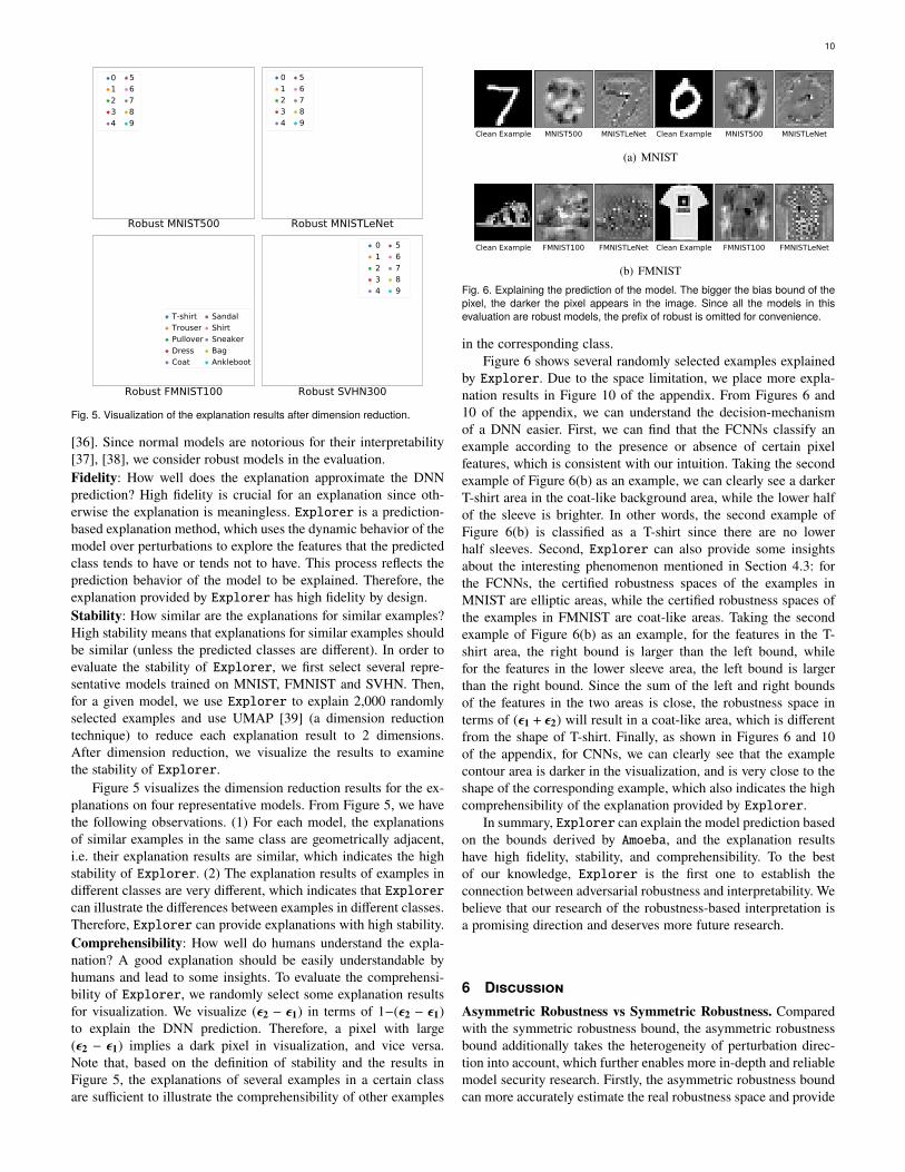
4.3 VisualizationNow, we visualize the asymmetric robustness bound (&1 + &2)to provide better understanding. In our visualization, we plot theasymmetric robustness bound in terms of 1 − (&1 + &2), and thusa small bounded space will result in a brighter visual perception.Notice that, according to the physical meaning of the asymmetricrobustness bound, a small bounded space also indicates the weakresistance against adversarial perturbations. Hence, these pixelswith small bounded space are critical for both model decision-making and model security.

Figure 4 visualizes the asymmetric robustness bounds ofseveral test examples. We can see from Figure 4 that, on the

1. Clean Example 2. MNIST500 3. Robust MNIST500 4. MNISTLeNet 5. Robust MNISTLeNet

(a) MNIST

1. Clean Example 2. FMNIST100 3. Robust FMNIST100 4. FMNISTLeNet 5. Robust FMNISTLeNet

(b) FMNISTFig. 4. Visualization of the asymmetric bounds of test examples on MNIST andFMNIST. Figures 4(a).2, 4(a).4, 4(b).2 and 4(b).4 represent the asymmetricbounds of the normal models, and Figures 4(a).3, 4(a).5, 4(b).3 and 4(b).5represent the asymmetric bounds of the robust models.

normal model, the shape of the input example and its boundedrobustness space are less related. Further, the robustness spacesof the pixels are very small, even for those that are not related todecision-making from the human’s view. This reveals that smallperturbations on those “unimportant" pixels can also fool thenormal model, making it not much robust.

For robust FCNNs, Figures 4(a).3 and 4(b).3 show the asym-metric robustness bounds of robust MNIST500 and robust FM-NIST100, respectively. From Figure 4(a).3, we can observe a largewhite elliptic area which implies that the robustness spaces of thepixels in this area are very small. It follows that small perturbationson these pixels will very likely cause misclassification of themodel, which is consistent with our human perception since theexample’s feature pixels are located in the elliptic area. Figure4(b).3 shows a white area with the shape of the coat, which is quitedifferent from the shape of the original example with the groundtruth label boot. In fact, we find a very interesting phenomenon:for robust FCNNs on MNIST (e.g., the robust MNIST500), theasymmetric robustness spaces of all the examples in MNIST areelliptic areas; while for robust FCNNs on FMNIST (e.g., therobust FMNIST100), the asymmetric robustness spaces of all theexamples in FMNIST are coat-like areas (see more examples inFigure 9 of the appendix). We will make more exploration andexplanation on this interesting phenomenon in Section 5.2.

For robust CNNs, the visualization results are more inter-pretable. We can clearly see the outline of 7 from Figure 4(a).5,and of a boot from Figure 4(b).5. These outlines are also criticalto our human decision-making.

In a word, through the above visualizations, we can find thatthe robust models are more interpretable than the normal models,and the CNNs are more interpretable than the FCNNs.

4.4 Robustness Space Analysis

In the state-of-the-art work [22], the authors certified the ro-bustness for FCNNs and found that the robustness space shapes(in terms of &) of different examples under the same model arehighly correlated and such correlation is even stronger underthe robust models. However, after we evaluate on more generalneural networks (e.g., CNNs) and analyze it more finely (e.g., theasymmetry), we find that such claim may not necessarily hold.

[22] used the pair-wise cosine similarity to measure suchcorrelation. Following [22], we first calculate the pair-wise cosine

8

similarity2 with respect to (&1 + &2) of 200 randomly selectedexamples. Then, we report the average cosine similarity as theresult.

The third column of Table 3 shows the average cosine simi-larity of the robustness space shapes. As shown in Table 3, thecosine similarity of the robustness spaces is very high, which isconsistent with [22]’s observation. For example, the average cosinesimilarity for the robust MNISTLeNet model is 0.9234, indicatinga high similarity. However, for the robust MNISTLeNet, the shapesof the asymmetric spaces of different examples are very different,as shown in Figure 9 of the appendix. In other words, they shouldnot have a high similarity from human’s perspective. In fact, thecosine similarity is a measure of direction similarity between twonon-zero vectors and the direction of a vector is mainly affected bythe large elements in it. However, the difference of two robustnessspaces mainly lies in the positions with small elements since thekey pixels tend to have small robustness space values. Even if therobustness spaces of different examples differ greatly, their cosinesimilarity is still very high, as supported by the results in Table3. Therefore, cosine similarity may not be a proper metric formeasuring the similarity of robustness space shapes.

Different from cosine similarity, the Wasserstein distance3can measure such difference. The Wasserstein distance for theasymmetric robustness bound can be intuitively understood as theminimum cost of changing from one robustness bound to another.A small Wasserstein distance implies a high geometric similarity.Therefore, we use the average pair-wise Wasserstein distancewithin the 200 examples’ certified robustness space to evaluatetheir shape correlation. For a more intuitive understanding of thesize of the Wasserstein distance, we also calculate the averagepair-wise Wasserstein distance within the example distributionsof different categories of MNIST, and the result is 0.045. Asshown in Table 3, we have the following observations. (1) Formost models, the large average Wasserstein distance indicateslarge difference between the robustness spaces. For example, theaverage Wasserstein distance 0.0573 of the robust MNISTLeNetdemonstrates the difference between robustness spaces is evenlarger than that between the examples of different categories.Therefore, the robustness space shapes of different examples underthe same model are not highly correlated. (2) For FCNNs, wefind that except for FMNIST100, the average Wasserstein distanceunder the robust model is smaller than that under the normalmodel, which is roughly consistent with [22]. However, for CNNs,we find that the average Wasserstein distance under the robustmodel is larger than that under the normal model. Therefore, undermore general network architectures, it is not suitable to think thatthe robustness space correlation of robust models is stronger thanthat of normal models.

The above correlation analysis is coarse-grained because itdoes not consider the asymmetry characteristic of the certifiedbounds. For a 1D case as an example, we assume that the asym-metric robustness bounds of two different examples are (&1 = 0.1,&2 = 0.2) and (&1 = 0.2, &2 = 0.1), respectively. In this case,the Wasserstein distance between the two examples in terms of(&2 + &1) is 0 even though they are different. Therefore, we use the

2. Cosine similarity is a measure of similarity between two non-zero vectorsof an inner product space that measures the cosine of the angle between them.3. The Wasserstein distance is defined as the cost of the optimal transport

plan for moving the mass in one distribution to another and provides a measureof the distance between two distributions. Different robustness spaces can beregarded as different distributions.

TABLE 3Cosine similarity and wasserstein distance of asymmetric robustness bounds.

Model Adversarial Training Average Cosine Average Wasserstein&2 + &1 &2 − &1

MNIST100 - 0.9602 0.0581 0.0429MNIST100 PGD 0.9926 0.0363 0.0672MNIST300 - 0.9788 0.0416 0.0387MNIST300 PGD 0.9964 0.0259 0.0594MNIST500 - 0.9832 0.0451 0.0389MNIST500 PGD 0.9968 0.0261 0.0758MNISTLeNet - 0.9304 0.0343 0.0673MNISTLeNet PGD 0.9234 0.0573 0.0826FMNIST100 - 0.8989 0.0724 0.0587FMNIST100 PGD 0.9724 0.1098 0.0657FMNISTLeNet - 0.7782 0.0209 0.1765FMNISTLeNet PGD 0.8726 0.1178 0.0668SVHN300 - 0.956 0.0692 0.042SVHN300 PGD 0.9928 0.0601 0.0686SVHNLeNet - 0.7822 0.0412 0.0778SVHNLeNet PGD 0.9764 0.0708 0.0897

average Wasserstein distance of (&2 − &1) for a more fine-grainedanalysis. In fact, (&2 − &1) can provide more detailed informationabout the asymmetry of the robustness space. The average pair-wise Wasserstein distance with respect to (&2 − &1) of the 200examples is shown in Table 3. As we can see from Table 3: (1) Theasymmetry of the robustness space shapes of different examplesunder the same model differ greatly. For example, the averageWasserstein distance is 0.067 and 0.0826 under the normal androbust MNISTLeNet, respectively, which indicates high differencein the asymmetry of robustness spaces. (2) The difference iseven stronger under the robust models. Specifically, the averageWasserstein distance of all the robust models now is greaterthan those of the normal models except for FMNISTLeNet. Wespeculate that such difference is related to the robustness againstuniversal adversarial perturbation [24]. This is also supported bythe observation that the robust models are more resistant againstuniversal adversarial perturbation [35]. It might be interesting toexplore the relationship between the robustness spaces of differentexamples and universal adversarial perturbation [24]. We will takethis as a future work.

In a word, through the above analysis on general network archi-tectures, we get a conclusion different from [22]: the robustnessspaces between different examples under the same model differgreatly, and the difference is even more significant under the robustmodel.

5 ApplicationIn this section, for demonstrating the superiority of the asym-

metric robustness bounds, we apply Amoeba in two security-related downstream tasks.5.1 Modeling Stronger Adversarial Threats

Amoeba can be used as a navigator to provide knowledge formodeling stronger adversarial threats. Usually, we can evaluate anattack using two criteria: (1) the evasion rate, i.e., the proportion ofthe generated adversarial examples that can fool the target model,and (2) the preserved utility, i.e., the similarity between an adver-sarial example and its corresponding clean example. Consideringthese two criteria, in this section, we employ Amoeba as a navigatorto enhance the utility of adversarial examples without reducing oreven improving the evasion rate (i.e., modeling stronger adversar-ial threats), and compare its effectiveness with the state-of-the-artsymmetric certification method [22]. For convenience, we denote

9

TABLE 4Evaluation results on MNIST.

Model Attacks Accuracy Distance;∞ ;0 ;2 ;1

MNIST100

FGSM (;∞), eps = 0.2 20.30% 0.2 (0) 393.7 (33.2) 4.17 (0.17) 88.05 (6.95)FGSMB(;∞), eps = 0.2 20.30% 0.2 (0) 393.7 (33.25) 4.17 (0.21) 88.05 (6.72)FGSM0(;∞), eps = 0.2 20.30% 0.2 (0) 375.1 (30.41) 4.08 (0.16) 84.32 (6.34)FGSM(;∞), eps = 0.3 9.15% 0.3 (0) 393.7 (35.3) 6.23 (0.26) 130.99 (10.8)FGSMB(;∞), eps = 0.3 9.15% 0.3 (0) 393.7 (35.5) 6.23 (0.27) 130.99 (11.4)FGSM0(;∞), eps = 0.3 9.15% 0.3 (0) 393.7 (34.7) 6.23 (0.21) 130.99 (11.9)PGD(;∞), eps=0.2 6.05% 0.2 (0) 405.1 (37.4) 3.99 (0.15) 83.72 (6.42)PGDB(;∞), eps=0.2 6.05% 0.2 (0) 405.1 (37.8) 3.99 (0.15) 83.72 (6.45)PGD0(;∞), eps=0.2 6.05% 0.2 (0) 405.1 (37.9) 3.99 (0.16) 83.72 (6.48)PGD(;2), eps=5.0 6.95% 0.86 (0.16) 452.8 (65.9) 4.97 (0.07) 83.7 (12.8)PGDB(;2), eps=5.0 4.80% 0.92 (0.19) 229.1 (44.87) 4.97 (0.06) 66.64 (5.39)PGD0(;2), eps=5.0 4.25% 0.92 (0.17) 229.1 (47.2) 4.97 (0.05) 66.65 (6.13)C&W(;2), ^ = 0 0.00% 0.3 (0.18) 377.6 (32.1) 1.62 (0.77) 25.45 (6.49)C&WB(;2), ^ = 0 0.00% 0.51 (0.31) 77.39 (9.12) 2.18 (1.01) 18.61 (7.33)C&W0(;2), ^ = 0 0.00% 0.48 (0.28) 70.32 (9.5) 2.08 (0.91) 18.21 (7.2)

MNISTLeNet

FGSM (;∞), eps = 0.2 67.95% 0.2 (0) 395.6 (39.7) 4.19 (0.19) 88.59 (7.63)FGSMB(;∞), eps = 0.2 67.95% 0.2 (0) 395.6 (40.1) 4.19 (0.18) 88.59 (7.52)FGSM0(;∞), eps = 0.2 67.95% 0.2 (0) 395.6 (37.4) 4.19 (0.18) 88.59 (7.54)FGSM(;∞),eps = 0.3 45.15% 0.3 (0) 395.6 (39.2) 6.26 (0.23) 131.8 (12.6)FGSMB(;∞), eps = 0.3 45.15% 0.3 (0) 395.6 (41.2) 6.26 (0.24) 131.8 (11.2)FGSM0(;∞), eps = 0.3 45.15% 0.3 (0) 395.6 (38.4) 6.26 (0.21) 131.8 (10.9)PGD(;∞), eps=0.2 38.75% 0.2 (0) 462.5 (42.3) 3.69 (0.16) 77.03 (6.54)PGDB(;∞), eps=0.2 38.75% 0.2 (0) 462.5 (40.3) 3.69 (0.15) 77.03 (6.07)PGD0(;∞), eps=0.2 38.75% 0.2 (0) 462.5 (40.5) 3.69 (0.16) 77.03 (7.09)PGD(;2), eps=5.0 20.84% 1.0 (0.34) 565.9 (94.5) 4.96 (0.11) 86.5 (17.6)PGDB(;2), eps=5.0 19.60% 1.25 (0.41) 126.5 (43.1) 4.91 (0.16) 47.53 (5.01)PGD0(;2), eps=5.0 15.35% 1.35 (0.38) 134.9 (35.8) 4.95 (0.08) 45.95 (6.14)C&W(;2), ^ = 0 0.00% 0.58 (0.28) 415.3 (38.2) 2.22 (0.92) 28.8 (11.2)C&WB(;2), ^ = 0 0.00% 0.87 (0.46) 72.64 (8.6) 2.79 (1.38) 22.71 (11.4)C&W0(;2), ^ = 0 0.00% 1.11 (0.36) 57.48 (8.12) 3.04 (1.45) 19.46 (9.82)

1 We use all the normal models from Section 4.2.2 as the target models. Refer to Tables 1, 5, 6, and 7 for more detailsabout the normal models.

2 The values in brackets denote the corresponding standard deviation, which is small compared to the correspondingdistance.

the certification method in [22] as Nonuniform in the followingdiscussion.

Intuitively, the pixels with smaller robustness spaces are morevulnerable to adversarial perturbations. Based on this, for generat-ing an adversarial example more effectively and efficiently, we canstart from manipulating the pixels with small robustness spaces.Specifically, given the robustness bound certified by Amoeba orNonuniform [22], we first select a certain proportion of pixelswith the smallest robustness spaces and then generate perturba-tions on those pixels using existing attacks. To ensure that theperturbations are generated only on those selected pixels, twomask matrices, whose elements corresponding to the selectedpixels are valid and otherwise invalid, can be used when gener-ating adversarial perturbations. We show the pseudo code of theenhanced attack in Algorithm 2, which is deferred in A of theappendix due to the space limitations.

To evaluate Algorithm 2, we mainly use three widely usedadversarial attacks: FGSM (;∞-based) [23], PGD (;2-based and;∞-based) [10], and the C&W (;2-based) attack [13]. Note that,Algorithm 2 can also be applied to enhance other adversarialattacks. We use �0 and �B to denote the enhanced version ofthe attack � based on Amoeba and Nonuniform, respectively,e.g, FGSM0 and FGSMB denote the enhanced version of FGSMbased on Amoeba and Nonuniform, respectively. The setting ofhyperparameters for all the attacks is summarized in Table 8 ofthe appendix. For each dataset, we use the original and enhancedattacks to generate adversarial examples, and then evaluate theirevasion rate (in terms of model accuracy) and utility (in terms of;1-distance).

Due to the space limitations, we only report partial results onMNIST here in Table 4. More experimental results on MNIST,FMNIST and SVHN are deferred to Tables 9, 10, and 11 in theappendix. From Tables 4, 9,10 and 11, we have the following ob-servations. (1) Without reducing the evasion rate, both Amoeba andNonuniform can help all the existing ;2-based attacks decreasethe total perturbation required to generate adversarial examples.For example, for MNISTLeNet, compared with C&W, C&WB andC&W0 decrease the total perturbations from 28.8 to 22.71 and19.46 respectively, while maintaining the evasion rate of 100%. (2)In some cases, both Amoeba and Nonuniform can even improve

the evasion rate. For example, for MNISTLeNet, compared withPGD (;2), PGDB (;2) and PGD0 (;2) not only decrease the totalperturbation from 86.5 to 47.53 and 42.95 respectively, but alsoreduce the model accuracy from 20.84% to 19.60% and 15.35%respectively. (3) Both Amoeba and Nonuniform cannot enhance;∞-based attacks in some cases. We speculate this is due to thelimitation of the added maximum perturbation on a single pixelin the ;∞-based attacks and so the robustness space cannot bebroken. An auxiliary evidence is that since there is no suchlimitation in ;2-based attacks, all the enhanced ;2-based attacksin Tables 4 9,10 and 11 not only reduce the total perturbations butalso remain or even improve the evasion rate. (4) For enhancingattacks, Amoeba is more effective than Nonuniform. Specifically,compared with Nonuniform-enhanced attacks, Amoeba-enhancedattacks can achieve the same success rate with less perturbations.For example, for MNISTLeNet, compared with C&WB , C&W0

decreases the total perturbations from 22.71 to 19.46. (5) Insome rare cases, compared with Nonuniform-enhanced attacks,Amoeba-enhanced attacks can achieve higher evasion rate withthe cost of slight larger total perturbations. For example, forMNIST100, compared with PGDB (;2), PGD0 (;2) decreases themodel accuracy from 4.80% to 4.25% while only increases theperturbation from 66.64 to 66.65, which is acceptable.

In summary, Amoeba can serve as a navigator to guide attacksto generate adversarial perturbations at the most vulnerable pixelpositions, thus enhancing their performance. According to theevaluation results, compared with the symmetric counterparts,Amoeba is more effective and efficient in modeling strongeradversarial threats.

5.2 Explaining the Prediction of DNNs

Understanding a DNN’s prediction is quite crucial for their usein security-related scenarios. In this section, we leverage Amoebato explain the DNN prediction. Similar to humans, DNNs alsoclassify examples according to the presence or absence of certainfeatures. For example, 7 and 1 can be distinguished according tothe presence or absence of the horizontal stroke. For images, thepresence of a feature comes from a large pixel value and viceversa. Therefore, increasing a pixel value implies a trend of afeature from absence to presence, and decreasing a pixel valueimplies a trend of a feature from presence to absence. For example,increasing the pixel values of the horizontal stroke in 1 (the trendof the horizontal stroke from absence to presence) will change 1to 7, i.e., 7 prefers to have the horizontal stroke. Based on this, wecan use Amoeba to explain the DNN prediction: if the predictedclass prefers to have a feature, the right bound of this feature islarger than its left bound since decreasing the feature value (thetrend of this feature from presence to absence) can easily resultin misclassification, and vice versa. It should be noted that suchexplanation cannot be provided by existing symmetric certificationmethods since they assume the left and right bounds are equal.

Specifically, we design a method called Explorer, which usesthe relative size of the left and right bounds to explain the DNNprediction. Given the asymmetric robustness bound certified byAmoeba, we perform (&2 − &1) and a feature with large (&2 − &1)means that the predicted class prefers to have this feature, andvice versa. Therefore, by visualizing (&2 − &1), we can identify thefeatures that the predicted class prefers to have. Below, we evaluatethe explanation provided by Explorer from three important andwidely used perspectives: fidelity, stability, and comprehensibility

10

Robust MNIST500

0

Robust MNISTLeNet

01234

56789

567894

321

Robust FMNIST100

T-shirtTrouserPulloverDressCoat

SandalShirtSneakerBagAnkleboot

Robust SVHN300

01234

56789

Fig. 5. Visualization of the explanation results after dimension reduction.

[36]. Since normal models are notorious for their interpretability[37], [38], we consider robust models in the evaluation.Fidelity: How well does the explanation approximate the DNNprediction? High fidelity is crucial for an explanation since oth-erwise the explanation is meaningless. Explorer is a prediction-based explanation method, which uses the dynamic behavior of themodel over perturbations to explore the features that the predictedclass tends to have or tends not to have. This process reflects theprediction behavior of the model to be explained. Therefore, theexplanation provided by Explorer has high fidelity by design.Stability: How similar are the explanations for similar examples?High stability means that explanations for similar examples shouldbe similar (unless the predicted classes are different). In order toevaluate the stability of Explorer, we first select several repre-sentative models trained on MNIST, FMNIST and SVHN. Then,for a given model, we use Explorer to explain 2,000 randomlyselected examples and use UMAP [39] (a dimension reductiontechnique) to reduce each explanation result to 2 dimensions.After dimension reduction, we visualize the results to examinethe stability of Explorer.

Figure 5 visualizes the dimension reduction results for the ex-planations on four representative models. From Figure 5, we havethe following observations. (1) For each model, the explanationsof similar examples in the same class are geometrically adjacent,i.e. their explanation results are similar, which indicates the highstability of Explorer. (2) The explanation results of examples indifferent classes are very different, which indicates that Explorercan illustrate the differences between examples in different classes.Therefore, Explorer can provide explanations with high stability.Comprehensibility: How well do humans understand the expla-nation? A good explanation should be easily understandable byhumans and lead to some insights. To evaluate the comprehensi-bility of Explorer, we randomly select some explanation resultsfor visualization. We visualize (&2 − &1) in terms of 1−(&2 − &1)to explain the DNN prediction. Therefore, a pixel with large(&2 − &1) implies a dark pixel in visualization, and vice versa.Note that, based on the definition of stability and the results inFigure 5, the explanations of several examples in a certain classare sufficient to illustrate the comprehensibility of other examples

Clean Example MNIST500 MNISTLeNet Clean Example MNIST500 MNISTLeNet

(a) MNIST

Clean Example FMNIST100 FMNISTLeNet Clean Example FMNIST100 FMNISTLeNet

(b) FMNISTFig. 6. Explaining the prediction of the model. The bigger the bias bound of thepixel, the darker the pixel appears in the image. Since all the models in thisevaluation are robust models, the prefix of robust is omitted for convenience.

in the corresponding class.Figure 6 shows several randomly selected examples explained

by Explorer. Due to the space limitation, we place more expla-nation results in Figure 10 of the appendix. From Figures 6 and10 of the appendix, we can understand the decision-mechanismof a DNN easier. First, we can find that the FCNNs classify anexample according to the presence or absence of certain pixelfeatures, which is consistent with our intuition. Taking the secondexample of Figure 6(b) as an example, we can clearly see a darkerT-shirt area in the coat-like background area, while the lower halfof the sleeve is brighter. In other words, the second example ofFigure 6(b) is classified as a T-shirt since there are no lowerhalf sleeves. Second, Explorer can also provide some insightsabout the interesting phenomenon mentioned in Section 4.3: forthe FCNNs, the certified robustness spaces of the examples inMNIST are elliptic areas, while the certified robustness spaces ofthe examples in FMNIST are coat-like areas. Taking the secondexample of Figure 6(b) as an example, for the features in the T-shirt area, the right bound is larger than the left bound, whilefor the features in the lower sleeve area, the left bound is largerthan the right bound. Since the sum of the left and right boundsof the features in the two areas is close, the robustness space interms of (&1 + &2) will result in a coat-like area, which is differentfrom the shape of T-shirt. Finally, as shown in Figures 6 and 10of the appendix, for CNNs, we can clearly see that the examplecontour area is darker in the visualization, and is very close to theshape of the corresponding example, which also indicates the highcomprehensibility of the explanation provided by Explorer.

In summary, Explorer can explain the model prediction basedon the bounds derived by Amoeba, and the explanation resultshave high fidelity, stability, and comprehensibility. To the bestof our knowledge, Explorer is the first one to establish theconnection between adversarial robustness and interpretability. Webelieve that our research of the robustness-based interpretation isa promising direction and deserves more future research.

6 DiscussionAsymmetric Robustness vs Symmetric Robustness. Comparedwith the symmetric robustness bound, the asymmetric robustnessbound additionally takes the heterogeneity of perturbation direc-tion into account, which further enables more in-depth and reliablemodel security research. Firstly, the asymmetric robustness boundcan more accurately estimate the real robustness space and provide

11

MNIST10

0

MNIST30

0

MNIST50

0

MNISTLeN

et

=10

MNIST10

0

MNIST30

0

MNIST50

0

MNISTLeN

et

0.0% 44.0% 51.0% 98.0%

6.5% 0.0% 25.5% 94.5%

5.0% 4.5% 0.0% 90.0%

90.5% 90.0% 90.0% 0.0%

MNIST10

0

MNIST30

0

MNIST50

0

MNISTLeN

et

=20

67.5% 72.5% 72.0% 0.0%

0.0% 0.0% 0.0% 57.0%

0.0% 0.0% 0.5% 78.5%

0.0% 6.0% 10.0% 91.0%

MNIST10

0

MNIST30

0

MNIST50

0

MNISTLeN

et

=30

46.0% 45.5% 51.5% 0.0%

0.0% 0.0% 0.0% 16.9%

0.0% 0.0% 0.0% 46.5%

0.0% 0.5% 1.0% 71.0%

MNIST10

0

MNIST30

0

MNIST50

0

MNISTLeN

et

=40

22.0% 19.5% 28.0% 0.0%

0.0% 0.0% 0.0% 2.0%

0.0% 0.0% 0.0% 13.0%

0.0% 0.0% 0.0% 46.0%

MNIST10

0

MNIST30

0

MNIST50

0

MNISTLeN

et

=50

0.0% 0.0% 0.0% 24.5%

0.0% 0.0% 0.0% 2.5%

0.0% 0.0% 0.0% 0.5%

12.0% 12.0% 11.5% 0.0%0%

25%

50%

75%

100%Cross-model Accuracy

Fig. 7. Cross-model accuracy of adversarial examples generated by the C&W attack on MNIST. The horizontal axis indicates the target model and the vertical axisindicates the corresponding surrogate model.

a quantitative robustness measurement regarding both the pertur-bation direction and magnitude, whereas the existing symmetricrobustness bound cannot provide such measurement regarding theperturbation direction. Secondly, the asymmetric robustness boundcan be more valuable and practical in safety-related tasks. Forexample, the asymmetric robustness can be used to explain modelpredictions and bridge the gap between adversarial robustnessand interpretability. Finally, through the asymmetric robustnessanalysis, it is possible for us to further improve the robustness of amodel. In the previous works [18], [19], their methods are equiv-alent to train robust models by maximizing min(n1, n2). However,this may limit further improvement on the model robustness sincethe inherent heterogeneity of perturbation direction. Different fromexisting works, we find a new insight that we can train a robustmodel by maximizing both n1 and n2 in each dimension. Takea simple 1D task as an example, where we need to decide themagnitude of a number. For simplicity, we assume that a numbergreater than 100 is a large number. For an input number 101, itsleft and right robustness bounds are 1 and +∞, respectively. Inprevious works [18], [19], their robust training method is to makethe model think that a number in (100, 102) is a large number.When considering the asymmetric robustness bounds, the robusttraining can make the model learn that a number in (100, 101+ n2)(n2 � 1 ) is a large number. Obviously, the latter helps the modellearn the essential features of a large number. Therefore, findingmodel parameters that maximize both n1 and n2 is helpful for themodel to learn the essential features of data examples. In this way,we are likely to obtain a more robust model with potentially betterutility. In a word, compared with the symmetric counterparts, theasymmetric robustness bound has better accuracy, reliability andpotential for many security applications.

Limitations and Future Works. As the first attempt to cer-tify the asymmetric robustness bounds for neural networks, webelieve our work can be improved from several aspects. Firstand foremost is extending the proposed method to certify therobustness bounds for larger models and more general networks(such as ResNets). The main challenge here is to tightly bound theoutput of the model. The second limitation is the efficiency issueof the proposed method, which could be further improved anddedicated research is necessary. Such research is also meaningfulfor obtaining more useful information and training more robustneural networks, especially for improving the model robustness ineach perturbation direction. Finally, there are correlations betweendifferent pixels. Specifically, when the value of a pixel changes, itpotentially affects the robustness bounds of other pixels. Therefore,how to determine this correlation and further take account of suchcorrelation to obtain a more accurate robustness space with a morecomplicated relaxation is an interesting future research direction.

7 Related Works

Adversarial Attacks and Defenses. DNNs are found to be vul-nerable to carefully perturbed input examples [5]. Recently, manyattacks have been proposed to generate adversarial examples.

As discussed in Section 2, FGSM takes one step to disturbthe original example. To enhance FGSM, many multi-step itera-tion methods based on FGSM are proposed, include PGD [10],BIM [8] and MI-FGSM [40]. Moosavi-Dezfooli et al. proposedanother iteration method called DeepFool [41] to minimize theadversarial perturbations. Papernot et al. proposed the Jacobian-based Saliency Map Approach (JSMA) [42] to efficiently generateadversarial examples, which utilizes the Jacobian matrix to calcu-late the saliency map of an input example, and then modifies asmall number of features based on the saliency map to deceive thetarget model. The C&W attack [13] includes three different attackalgorithms, which make the perturbations almost imperceptible bylimiting the ;∞, ;2 and ;0 distance between the adversarial exampleand the original example, and can control the confidence of thegenerated adversarial examples. Tramer et al. explored the spaceof transferable adversarial attacks and proposed a method whichmeasures the dimensionality of the adversarial subspace [43].

On the other side, to improve the robustness of neural networksagainst adversarial attacks, researchers have proposed variousdefense methods. Madry et al. proposed adversarial training [10],which is to add adversarial examples constantly in the process ofmodel training and build a model with better robustness. Adversar-ial training mainly includes naive adversarial training [8], ensem-ble adversarial training [9], and PGD-based adversarial training[10]. Papernot et al. proposed a distillation training method nameddefensive distillation [7]. Meng et al. proposed Magnet [44] thatuses auto-encoder to improve the model robustness. PixelDefense[45] uses the generated model PixelCNN to transform the adver-sarial examples into the normal example space, and then feedsthe transformed examples into the original model for prediction.However, these defense methods usually were broken soon bynew stronger attacks [12], [13], [34], and the long-term arms racebetween adversarial attack and defense continues, motivating theemerging robustness certification research, including this work.Robustness Certification. Existing robustness certification tech-niques generally can be divided into two categories: completemethods, which can certify the exact robustness bound but com-putationally expensive, and incomplete methods, which can certifythe approximate robustness bound but easy to scale.

For the complete methods, many use Satisfiability ModuloTheories (SMT) ( [14], [15], [16], [17]) to certify the robustnessof neural networks against adversarial attacks. In addition, integerprogramming approaches [46], [47], [48] are utilized to verify therobustness. However, they can only be used to certify networks

12

with small sizes, i.e., limited number of layers and neurons, due tothe computation cost.

There have also been a number of recent works to certify neu-ral networks via incomplete methods. Wong et al. [18], [19] useda convex polytope relaxation to bound the robust error or loss thatcan be reached under norm-bounded perturbation. Raghunathanet al. [20], [21] leveraged Semi-Definite Programming (SDP)relaxation to approximate the adversarial polytope and employedthis to train a robust model. Abstract interpretation is also usedto verifying neural networks, which can soundly approximatethe behavior of neural networks ( [32], [49], [50], [51], [52]).More recently, another line of work considers certifying modelrobustness via randomized smoothing [53], [54]. They provideprobabilistic robustness guarantees for smoothed models whosepredictions cannot be evaluated exactly, only approximated toarbitrarily high confidence. The above methods are verifying auniform bound of a test example. To get a more realistic bound,Liu et al. [22] proposed a framework to get the non-uniform boundof a test example. They showed that the non-uniform bounds havelarger volumes than that of the uniform bounds. However, theproposed non-uniform bound ignores the inherent heterogeneityof the perturbation direction and it was only evaluated on FCNNs.

Different from existing research, first, Amoeba accounts forthe heterogeneity of perturbation direction and estimates the realrobustness space in a more precise manner. Second, we evaluateour method on more general networks (such as CNNs) alongwith interesting findings. Finally, we also investigate the broadapplications of the robustness space for downstream security-related tasks.

8 ConclusionIn this paper, we present Amoeba, the first-of-its-kind frame-

work that efficiently certifies the asymmetric robustness of DNNs.Compared with the alternative certification methods in prior work,Amoeba provides quantitative robustness measures with respectto both perturbation direction and magnitude, and estimates suchbounds in a more precise manner. We further show that asymmet-ric robustness entails many security-related use cases including(i) modeling stronger adversarial threats, (ii) explaining DNNpredictions, leading to several promising directions for furtherresearch.AcknowledgmentThis work was partly supported by the National Key Research andDevelopment Program of China under No. 2020AAA0140004, theZhejiang Provincial Natural Science Foundation for DistinguishedYoung Scholars under No. LR19F020003, and NSFC under No.61772466 and U1836202.

References[1] B. Zhao, H. Weng, S. Ji, J. Chen, T. Wang, Q. He, and R. Beyah,

“Towards evaluating the security of real-world deployed image captchas,”in Proceedings of the 11th ACM Workshop on Artificial Intelligence andSecurity, 2018, pp. 85–96.

[2] K. He, X. Zhang, S. Ren, and J. Sun, “Deep residual learning for imagerecognition,” in Proceedings of the IEEE conference on computer visionand pattern recognition, 2016, pp. 770–778.

[3] Y. Sun, X. Wang, and X. Tang, “Sparsifying neural network connectionsfor face recognition,” in Proceedings of the IEEE Conference on Com-puter Vision and Pattern Recognition, 2016, pp. 4856–4864.

[4] A. Graves, A.-r. Mohamed, and G. Hinton, “Speech recognition withdeep recurrent neural networks,” in 2013 IEEE international conferenceon acoustics, speech and signal processing. IEEE, 2013, pp. 6645–6649.

[5] C. Szegedy, W. Zaremba, I. Sutskever, J. Bruna, D. Erhan, I. Goodfellow,and R. Fergus, “Intriguing properties of neural networks,” arXiv preprintarXiv:1312.6199, 2013.

[6] I. Evtimov, K. Eykholt, E. Fernandes, B. Li, A. Rahmati, C. Xiao,A. Prakash, T. Kohno, and D. Song, “Robust physical-world attacks ondeep learning visual classification,” in CVPR, 2018.

[7] N. Papernot, P. McDaniel, X. Wu, S. Jha, and A. Swami, “Distillation asa defense to adversarial perturbations against deep neural networks,” in2016 IEEE Symposium on Security and Privacy (SP). IEEE, 2016, pp.582–597.

[8] A. Kurakin, I. Goodfellow, and S. Bengio, “Adversarial machine learningat scale,” arXiv preprint arXiv:1611.01236, 2016.

[9] F. Tramèr, A. Kurakin, N. Papernot, I. Goodfellow, D. Boneh, andP. McDaniel, “Ensemble adversarial training: Attacks and defenses,”arXiv preprint arXiv:1705.07204, 2017.

[10] A. Madry, A. Makelov, L. Schmidt, D. Tsipras, and A. Vladu, “Towardsdeep learning models resistant to adversarial attacks,” arXiv preprintarXiv:1706.06083, 2017.

[11] X. Cao and N. Z. Gong, “Mitigating evasion attacks to deep neuralnetworks via region-based classification,” in Proceedings of the 33rdAnnual Computer Security Applications Conference. ACM, 2017, pp.278–287.

[12] N. Carlini and D. Wagner, “Magnet and" efficient defenses against ad-versarial attacks" are not robust to adversarial examples,” arXiv preprintarXiv:1711.08478, 2017.

[13] ——, “Towards evaluating the robustness of neural networks,” in 2017IEEE Symposium on Security and Privacy. IEEE, 2017, pp. 39–57.

[14] X. Huang, M. Kwiatkowska, S. Wang, and M. Wu, “Safety verification ofdeep neural networks,” in International Conference on Computer AidedVerification. Springer, 2017, pp. 3–29.

[15] G. Katz, C. Barrett, D. L. Dill, K. Julian, and M. J. Kochenderfer,“Reluplex: An efficient smt solver for verifying deep neural networks,”in International Conference on Computer Aided Verification. Springer,2017, pp. 97–117.

[16] R. Ehlers, “Formal verification of piece-wise linear feed-forward neuralnetworks,” in International Symposium on Automated Technology forVerification and Analysis. Springer, 2017, pp. 269–286.

[17] N. Carlini, G. Katz, C. Barrett, and D. L. Dill, “Ground-truth adversarialexamples,” arXiv preprint arXiv:1709.10207, 2017.

[18] E. Wong, F. Schmidt, J. H. Metzen, and J. Z. Kolter, “Scaling provableadversarial defenses,” in Advances in Neural Information ProcessingSystems, 2018, pp. 8400–8409.

[19] E. Wong and J. Z. Kolter, “Provable defenses against adversarialexamples via the convex outer adversarial polytope,” arXiv preprintarXiv:1711.00851, 2017.

[20] A. Raghunathan, J. Steinhardt, and P. Liang, “Certified defenses againstadversarial examples,” arXiv preprint arXiv:1801.09344, 2018.

[21] A. Raghunathan, J. Steinhardt, and P. S. Liang, “Semidefinite relaxationsfor certifying robustness to adversarial examples,” in Advances in NeuralInformation Processing Systems, 2018, pp. 10 877–10 887.

[22] C. Liu, R. Tomioka, and V. Cevher, “On certifying non-uniform boundagainst adversarial attacks,” ICML, 2019.

[23] I. J. Goodfellow, J. Shlens, and C. Szegedy, “Explaining and harnessingadversarial examples,” arXiv preprint arXiv:1412.6572, 2014.

[24] S.-M. Moosavi-Dezfooli, A. Fawzi, O. Fawzi, and P. Frossard, “Universaladversarial perturbations,” in Proceedings of the IEEE conference oncomputer vision and pattern recognition, 2017, pp. 1765–1773.

[25] T.-W. Weng, H. Zhang, H. Chen, Z. Song, C.-J. Hsieh, L. Daniel, D. Bon-ing, and I. Dhillon, “Towards fast computation of certified robustness forrelu networks,” in International Conference on Machine Learning, 2018,pp. 5273–5282.

[26] M. R. Hestenes, “Multiplier and gradient methods,” Journal of optimiza-tion theory and applications, vol. 4, no. 5, pp. 303–320, 1969.

[27] M. J. Powell, “A fast algorithm for nonlinearly constrained optimizationcalculations,” in Numerical analysis. Springer, 1978, pp. 144–157.

[28] Y. LeCun, L. Bottou, Y. Bengio, P. Haffner et al., “Gradient-basedlearning applied to document recognition,” Proceedings of the IEEE,vol. 86, no. 11, pp. 2278–2324, 1998.

[29] H. Xiao, K. Rasul, and R. Vollgraf, “Fashion-mnist: a novel imagedataset for benchmarking machine learning algorithms,” arXiv preprintarXiv:1708.07747, 2017.

[30] Y. Netzer, T. Wang, A. Coates, A. Bissacco, B. Wu, and A. Y. Ng,“Reading digits in natural images with unsupervised feature learning,” inNIPS Workshop on Deep Learning and Unsupervised Feature Learning2011, 2011.

[31] X. Zhang, N. Wang, H. Shen, S. Ji, X. Luo, and T. Wang, “Interpretabledeep learning under fire,” in USENIX Security, 2020.

13

[32] G. Singh, T. Gehr, M. Mirman, M. Püschel, and M. Vechev, “Fast andeffective robustness certification,” in Advances in Neural InformationProcessing Systems, 2018, pp. 10 802–10 813.

[33] A. Shafahi, M. Najibi, A. Ghiasi, Z. Xu, J. Dickerson, C. Studer, L. S.Davis, G. Taylor, and T. Goldstein, “Adversarial training for free!” arXivpreprint arXiv:1904.12843, 2019.

[34] A. Athalye, N. Carlini, and D. Wagner, “Obfuscated gradients give afalse sense of security: Circumventing defenses to adversarial examples,”arXiv preprint arXiv:1802.00420, 2018.

[35] C. K. Mummadi, T. Brox, and J. H. Metzen, “Defending against universalperturbations with shared adversarial training,” in Proceedings of theIEEE International Conference on Computer Vision, 2019, pp. 4928–4937.

[36] C. Molnar, Interpretable Machine Learning: A Guide for Making BlackBox Models Explainable., 2019.

[37] A. S. Ross and F. Doshi-Velez, “Improving the adversarial robustnessand interpretability of deep neural networks by regularizing their inputgradients,” in Thirty-second AAAI conference on artificial intelligence,2018.

[38] D. Tsipras, S. Santurkar, L. Engstrom, A. Turner, and A. Madry, “Robust-ness may be at odds with accuracy,” arXiv preprint arXiv:1805.12152,2018.

[39] L. McInnes, J. Healy, and J. Melville, “UMAP: Uniform ManifoldApproximation and Projection for Dimension Reduction,” arXiv preprintarXiv:1802.03426, 2018.

[40] Y. Dong, F. Liao, T. Pang, H. Su, J. Zhu, X. Hu, and J. Li, “Boostingadversarial attacks with momentum,” in Proceedings of the IEEE confer-ence on computer vision and pattern recognition, 2018, pp. 9185–9193.

[41] S.-M. Moosavi-Dezfooli, A. Fawzi, and P. Frossard, “Deepfool: a simpleand accurate method to fool deep neural networks,” in Proceedings of theIEEE conference on computer vision and pattern recognition, 2016, pp.2574–2582.

[42] N. Papernot, P. McDaniel, S. Jha, M. Fredrikson, Z. B. Celik, andA. Swami, “The limitations of deep learning in adversarial settings,” in2016 IEEE European Symposium on Security and Privacy (EuroS&P).IEEE, 2016, pp. 372–387.

[43] F. Tramèr, N. Papernot, I. Goodfellow, D. Boneh, and P. McDaniel,“The space of transferable adversarial examples,” arXiv preprintarXiv:1704.03453, 2017.

[44] D. Meng and H. Chen, “Magnet: a two-pronged defense against adver-sarial examples,” in Proceedings of the 2017 ACM SIGSAC Conferenceon Computer and Communications Security. ACM, 2017, pp. 135–147.

[45] Y. Song, T. Kim, S. Nowozin, S. Ermon, and N. Kushman, “Pixeldefend:Leveraging generative models to understand and defend against adversar-ial examples,” arXiv preprint arXiv:1710.10766, 2017.

[46] A. Lomuscio and L. Maganti, “An approach to reachability analysis forfeed-forward relu neural networks,” arXiv preprint arXiv:1706.07351,2017.

[47] V. Tjeng, K. Xiao, and R. Tedrake, “Evaluating robustness ofneural networks with mixed integer programming,” arXiv preprintarXiv:1711.07356, 2017.

[48] C.-H. Cheng, G. Nührenberg, and H. Ruess, “Maximum resilience ofartificial neural networks,” in International Symposium on AutomatedTechnology for Verification and Analysis. Springer, 2017, pp. 251–268.

[49] T. Gehr, M. Mirman, D. Drachsler-Cohen, P. Tsankov, S. Chaudhuri, andM. Vechev, “Ai2: Safety and robustness certification of neural networkswith abstract interpretation,” in 2018 IEEE Symposium on Security andPrivacy (SP). IEEE, 2018, pp. 3–18.

[50] M. Mirman, T. Gehr, and M. Vechev, “Differentiable abstract interpreta-tion for provably robust neural networks,” in International Conference onMachine Learning, 2018, pp. 3575–3583.

[51] G. Singh, T. Gehr, M. Püschel, and M. Vechev, “An abstract domain forcertifying neural networks,” Proceedings of the ACM on ProgrammingLanguages, vol. 3, no. POPL, pp. 1–30, 2019.

[52] M. Mirman, G. Singh, and M. Vechev, “A provable defense for deepresidual networks,” arXiv preprint arXiv:1903.12519, 2019.

[53] J. Cohen, E. Rosenfeld, and Z. Kolter, “Certified adversarial robustnessvia randomized smoothing,” in International Conference on MachineLearning. PMLR, 2019, pp. 1310–1320.

[54] J. Jia, X. Cao, B. Wang, and N. Z. Gong, “Certified robustness for top-kpredictions against adversarial perturbations via randomized smoothing,”arXiv preprint arXiv:1912.09899, 2019.

14

Appendix.1 AlgorithmsIn this section, we show the pseudo code of modeling strongeradversarial threats mentioned in 5.1.

Algorithm 2: Modeling Stronger Adversarial ThreatsInput: ?: proportion of disturbed pixels;�: the robustness bound;�: the attack algorithm;-, H: the input examples and labels;Output: Adversarial Examples: -03E

1 Initialize the attack examples -03E ← - ;2 repeat3 Store attack from previous iteration: - ← -03E ;4 Generate mask "1,"2 based on ? and �;5 Update step: -03E ←

"1 � [(�(-, H) − -)]+ +"2 � [(�(-, H) − -)]− + - ,where �(-, H) − - is the adversarial perturbationsbased on the given attack algorithm;

6 until successful attack;

.2 Experimental SetupIn this section, we show the experimental setup information,including the configuration of training, model architecture, andattack hyperparameters.

TABLE 5Configuration for Normal and Adversarial Training

Hyperparameters Normal Training Adversarial TrainingBathch Size 100 100Epochs 100 100

Optimizer Adam AdamLearning Rate 1e-4 1e-4

Attack - PGDU 0.005n 0.1= 20

TABLE 6Model Architecture of Fully-connected Neural Networks

ArchitectureModel

MNIST100FMNIST100

MNIST300FMNIST300

MNIST500FMNIST500

Input Layer 784 784 784Hidden Layer1 FC(100)+ReLU FC(300)+ReLU FC(500)+ReLUHidden Layer2 FC(100)+ReLU FC(300)+ReLU FC(500)+ReLUHidden Layer3 FC(100)+ReLU FC(300)+ReLU FC(500)+ReLUOutput Layer 10 10 10

TABLE 7Model Architecture of Convolutional Neural Networks

Architecture ModelMNISTLeNetFMNISTLeNet SVHNLeNet

Input Layer (1,28,28) (3,32,32)

Hidden Layer1Conv(1,6,3,1,1)

ReLUMaxPool(2,2)

Conv(3,6,3,1,1)ReLu

MaxPool(2,2)

Hidden Layer2Conv(6,16,5,1,0)

ReLUMaxPool(2,2)

Conv(6,16,5,1,0)ReLu

MaxPool(2,2)Hidden Layer3 Flatten FlattenHidden Layer4 FC(120)+ReLU FC(120)+ReLUHidden Layer5 FC(84)+ReLU FC(84)+ReLUOutput Layer 10 10

TABLE 8Attack Hyperparameters

Dataset Attacks Hyperparameters

MNIST, FMNISTFGSM, FGSMB , FGSM0 ;∞:n = 0.2 and 0.3

PGD, PGDB , PGD0;∞:n = 0.2, U = 0.015;2: n = 5.0, U = 0.5

n=20C&W, C&WB , C&W0 ^=0

SVHNFGSM, FGSMB , FGSM0 ;∞:n = 0.2 and 0.3

PGD, PGDB , PGD0;∞:n = 0.2, U = 0.015;2: n = 10.0, U = 0.5

n=20C&W, C&WB , C&W0 ;2: n = 5.0, U = 0.5

.3 More Experimental Results

In this section, we show more experimental results.

TABLE 9Evaluation Results on MNIST


MNIST100

FGSM (;∞), eps = 0.2 20.30% 0.2 393.7 4.17 88.05FGSMB(;∞), eps = 0.2 20.30% 0.2 393.7 4.17 88.05FGSM0(;∞), eps = 0.2 20.30% 0.2 375.1 4.08 84.32FGSM(;∞), eps = 0.3 9.15% 0.3 393.7 6.23 130.99FGSMB(;∞), eps = 0.3 9.15% 0.3 393.7 6.23 130.99FGSM0(;∞), eps = 0.3 9.15% 0.3 393.7 6.23 130.99PGD(;∞), eps=0.2 6.05% 0.2 405.1 3.99 83.72PGDB(;∞), eps=0.2 6.05% 0.2 405.1 3.99 83.72PGD0(;∞), eps=0.2 6.05% 0.2 405.1 3.99 83.72PGD(;2), eps=5.0 6.95% 0.86 452.8 4.97 83.7PGDB(;2), eps=5.0 4.80% 0.92 229.1 4.97 66.64PGD0(;2), eps=5.0 4.25% 0.92 229.1 4.97 66.65C&W(;2), ^ = 0 0.00% 0.3 377.6 1.62 25.45C&WB(;2), ^ = 0 0.00% 0.51 77.39 2.18 18.61C&W0(;2), ^ = 0 0.00% 0.48 70.32 2.08 18.21

MNIST300

FGSM (;∞), eps = 0.2 26.45% 0.2 383.6 4.14 86.47FGSMB(;∞), eps = 0.2 26.45% 0.2 383.6 4.14 86.47FGSM0(;∞), eps = 0.2 26.45% 0.2 383.6 4.14 86.47FGSM(;∞),eps = 0.3 8.95% 0.3 383.6 6.17 128.63FGSMB(;∞), eps = 0.3 8.95% 0.3 383.6 6.17 128.63FGSM0(;∞), eps = 0.3 8.95% 0.3 383.6 6.17 128.63PGD(;∞), eps=0.2 11.25% 0.2 402.3 4.01 84.16PGDB(;∞), eps=0.2 11.25% 0.2 402.3 4.01 84.16PGD0(;∞), eps=0.2 11.25% 0.2 402.3 4.01 84.16PGD(;2), eps=5.0 11.90% 0.88 482.8 4.97 85.93PGDB(;2), eps=5.0 9.85% 1.39 53.78 4.97 33.51PGD0(;2), eps=5.0 8.70% 1.31 52.9 4.97 35.35C&W(;2), ^ = 0 0.00% 0.38 376.3 1.89 28.89C&WB(;2), ^ = 0 0.00% 0.59 77.7 2.37 20.69C&W0(;2), ^ = 0 0.00% 0.54 72.72 2.27 20.48

MNIST500


MNISTLeNet


1 We take all the normal models trained on Section 4.2.2 as the target models. Refer toTables 1, 5, and 6, 7 for more details about the normal models.

2 For simplicity, we omit the standard deviation since it’s small value.

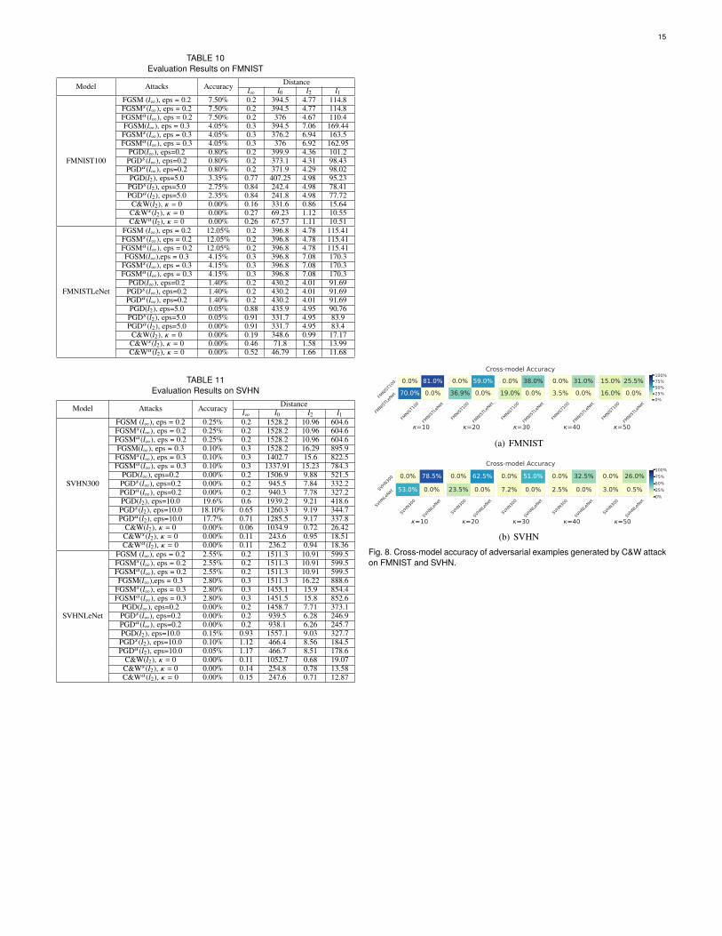
15

TABLE 10Evaluation Results on FMNIST


FMNIST100

FGSM (;∞), eps = 0.2 7.50% 0.2 394.5 4.77 114.8FGSMB(;∞), eps = 0.2 7.50% 0.2 394.5 4.77 114.8FGSM0(;∞), eps = 0.2 7.50% 0.2 376 4.67 110.4FGSM(;∞), eps = 0.3 4.05% 0.3 394.5 7.06 169.44FGSMB(;∞), eps = 0.3 4.05% 0.3 376.2 6.94 163.5FGSM0(;∞), eps = 0.3 4.05% 0.3 376 6.92 162.95PGD(;∞), eps=0.2 0.80% 0.2 399.9 4.36 101.2PGDB(;∞), eps=0.2 0.80% 0.2 373.1 4.31 98.43PGD0(;∞), eps=0.2 0.80% 0.2 371.9 4.29 98.02PGD(;2), eps=5.0 3.35% 0.77 407.25 4.98 95.23PGDB(;2), eps=5.0 2.75% 0.84 242.4 4.98 78.41PGD0(;2), eps=5.0 2.35% 0.84 241.8 4.98 77.72C&W(;2), ^ = 0 0.00% 0.16 331.6 0.86 15.64C&WB(;2), ^ = 0 0.00% 0.27 69.23 1.12 10.55C&W0(;2), ^ = 0 0.00% 0.26 67.57 1.11 10.51

FMNISTLeNet


TABLE 11Evaluation Results on SVHN


SVHN300


SVHNLeNet


FMNIST

100

FMNIST

LeNet

=10

FMNIST

100

FMNIST

LeNet

0.0% 81.0%70.0% 0.0%

FMNIST

100

FMNIST

LeNet

=20

36.9% 0.0%0.0% 59.0%

FMNIST

100

FMNIST

LeNet

=30

19.0% 0.0%0.0% 38.0%

FMNIST

100

FMNIST

LeNet

=40

3.5% 0.0%0.0% 31.0%

FMNIST

100

FMNIST

LeNet

=50

15.0% 25.5%16.0% 0.0%

0%25%50%75%100%

Cross-model Accuracy

(a) FMNIST

SVHN30

0

SVHNLeN

et

=10

SVHN30

0

SVHNLeN

et

0.0% 78.5%

53.0% 0.0%

SVHN30

0

SVHNLeN

et

=20

23.5% 0.0%

0.0% 62.5%

SVHN30

0

SVHNLeN

et

=30

7.2% 0.0%

0.0% 51.0%

SVHN30

0

SVHNLeN

et

=40

2.5% 0.0%

0.0% 32.5%

SVHN30

0

SVHNLeN

et

=50

0.0% 26.0%

3.0% 0.5%0%25%50%75%100%

Cross-model Accuracy

(b) SVHNFig. 8. Cross-model accuracy of adversarial examples generated by C&W attackon FMNIST and SVHN.

16

Original Example MNIST100 Robust MNIST100 Original Example MNIST100 Robust MNIST100



Original Example MNISTLeNet Robust MNISTLeNet Original Example MNISTLeNet Robust MNISTLeNet

Original Example FMNIST100 Robust FMNIST100 Original Example FMNIST100 Robust FMNIST100

Original Example FMNISTLeNet Robust FMNISTLeNet Original Example FMNISTLeNet Robust FMNISTLeNetFig. 9. Visualization of the asymmetric robustness bounds of examples on MNIST and FMNIST.

17

Clean Example MNIST500 MNISTLeNet Clean Example MNIST500 MNISTLeNet Clean Example FMNIST100 FMNISTLeNet Clean Example FMNIST100 FMNISTLeNet










Fig. 10. Explanation results on MNIST and FMNIST.

18

Changjiang Li is currently a Ph.D. student in the Col-lege of Information Science and Technology at Penn-sylvania State University. He received the Master de-gree from the School of Computer Science at ZhejiangUniversity in 2020. His research interest includes Ad-versarial Machine Learning, AI privacy.

Shouling Ji is a ZJU 100-Young Professor in the Col-lege of Computer Science and Technology at ZhejiangUniversity and a Research Faculty in the School ofElectrical and Computer Engineering at Georgia Insti-tute of Technology. He received a Ph.D. in Electricaland Computer Engineering from Georgia Institute ofTechnology, a Ph.D. in Computer Science from Geor-gia State University. His current research interests in-clude AI Security, Data-driven Security, Privacy andData Analytics. He is a member of IEEE and ACMand was the Membership Chair of the IEEE Student

Branch at Georgia State (2012- 2013).

HaiqinWeng is with the Ant Group, Hangzhou, China.Her research interests include AI security, anomaly de-tection, and machine learning. She received her Ph.D.degree in College of Computer Science and Technol-ogy at Zhejiang University in 2019, and received herBS degree from South China University of Technologyin 2014.

Bo Li is currently an Assistant Professor with the De-partment of Computer Science, University of Illinois atUrbana–Champaign. She has designed several robustlearning algorithms against adversarial behaviors, ascalable framework for achieving robustness for arange of learning methods, and a privacy preservingdata publishing systems. Her research interests in-clude theoretical and practical aspects of security, ma-chine learning, privacy, game theory, adversarial deeplearning, generative models, and designing scalablerobust machine learning models against unrestricted

adversarial attacks. Her work has been featured by major publications andmediaoutlets, such as Nature, Wired, Fortune, and the IEEE Spectrum. She was arecipient of the Symantec Research Labs Fellowship and the MIT TechnologyReview TR-35 Award.

Jie Shi is a Principal Researcher in Huawei SingaporeResearch Center. His research interests include trust-worthy AI, machine learning security, data security andprivacy, IoT security and applied cryptography. He hasover 10 years’ research experience and has publishedover 30 research papers in refereed journals and in-ternational conferences. He received his Ph.D degreefrom Huazhong University of Science and Technology,China.

Raheem Beyah, a native of Atlanta, GA, serves asGeorgia Tech’s Vice President for Interdisciplinary Re-search, Executive Director of the OnlineMasters of Cy-bersecurity program (OMS Cybersecurity), and is theMotorola Foundation Professor in School of Electricaland Computer Engineering. He is also Co-Founder ofFortiphyd Logic , Inc. Raheem received his Bachelor ofScience in Electrical Engineering from North CarolinaA&T State University in 1998. He received his Mas-ters and Ph.D. in Electrical and Computer Engineeringfrom Georgia Tech in 1999 and 2003, respectively.

His research interests include Network security and monitoring, Cyber-physicalSystems Security, Network traffic characterization and performance, and Criticalinfrastructure security. He received the National Science Foundation CAREERaward in 2009 and was selected for DARPA’s Computer Science Study Panel in2010. He is a member of AAAS, ASEE, a lifetime member of NSBE, a seniormember of IEEE, and an ACM Distinguished Scientist.

ShanqingGuo is currently a professor with the Schoolof Cyber Science and Technology at Shandong Uni-versity. He received his M.S. and Ph.D. degrees incomputer science from Ocean University, China, in2003, and Nanjing University, China, in 2006 respec-tively. He joined the School of Computer Science andTechnology at Shandong University as an assistantprofessor in 2006. His research interests include AISecurity, Software and System Security. He has pub-lished in S&P, ICDE, ACSAC, RAID, DSN, CIKM, IC-SME, ISSRE and other venues. He also serves as a

program committee member or a reviewer for various international conferencesand journals, e.g., ISSRE, ICSME and Computer&Security.

Zonghui Wang is a senior engineer in the college ofComputer Science and Engineering at Zhejiang Uni-versity in Hangzhou, China. He received his Ph.D.in the college of Computer Science and Engineeringat Zhejiang University in 2007. His current researchinterests focus on deep learning, AI security, cloudcomputing and computer architecture.

Ting Wang received the Ph.D. degree from the Geor-gia Institute of Technology. He is currently an AssistantProfessor with the College of Information Science andTechnology, Pennsylvania State University. He con-ducts research at the intersection of machine learningand privacy and security. His ongoing work focuseson making machine learning systems more practicallyusable through mitigating security vulnerabilities, en-hancing privacy awareness, and increasing decision-making transparency.

TowardsCertifyingtheAsymmetricRobustnessfor NeuralNetworks ...

Documents

Transcript of TowardsCertifyingtheAsymmetricRobustnessfor NeuralNetworks ...