Neural Networks and the BiadVariance Dilemma
58
VIEW Communicated by Lawrence Jackel Neural Networks and the BiadVariance Dilemma Stuart Geman Division of Applied Mathematics, Brown University, Providence, XI 02912 USA Elie Bienenstock RenC Doursat ESPCI, 10 rue Vuuquelin, 75005 Paris, France Feedforward neural networks trained by error backpropagation are ex- amples of nonparametric regression estimators. We present a tutorial on nonparametric inference and its relation to neural networks, and we use the statistical viewpoint to highlight strengths and weaknesses of neural models. We illustrate the main points with some recognition experiments involving artificial data as well as handwritten numer- als. In way of conclusion, we suggest that current-generation feed- forward neural networks are largely inadequate for difficult problems in machine perception and machine learning, regardless of parallel- versus-serial hardware or other implementation issues. Furthermore, we suggest that the fundamental challenges in neural modeling are about representation rather than learning per se. This last point is supported by additional experiments with handwritten numerals. 1 Introduction Much of the recent work on feedforward artificial neural networks brings to mind research in nonparametric statistical inference. This is a branch of statistics concerned with model-free estimation, or, from the biological viewpoint, tabula rasa learning. A typical nonparametric inference prob- lem is the learning (or “estimating,” in statistical jargon) of arbitrary decision boundaries for a classification task, based on a collection of la- beled (pre-classified) training samples. The boundaries are arbitrary in the sense that no particular structure, or class of boundaries, is assumed a priori. In particular, there is no parametric model, as there would be with a presumption of, say, linear or quadratic decision surfaces. A similar point of view is implicit in many recent neural network formulations, suggesting a close analogy to nonparametric inference. Of course statisticians who work on nonparametric inference rarely concern themselves with the plausibility of their inference algorithms Neural Computation 4,l-58 (1992) @ 1992 Massachusetts Institute of Technology
Transcript of Neural Networks and the BiadVariance Dilemma
VIEW Communicated by Lawrence Jackel
Neural Networks and the BiadVariance Dilemma
Stuart Geman Division of Applied Mathematics, Brown University, Providence, XI 02912 USA
Elie Bienenstock RenC Doursat ESPCI, 10 rue Vuuquelin, 75005 Paris, France
Feedforward neural networks trained by error backpropagation are ex- amples of nonparametric regression estimators. We present a tutorial on nonparametric inference and its relation to neural networks, and we use the statistical viewpoint to highlight strengths and weaknesses of neural models. We illustrate the main points with some recognition experiments involving artificial data as well as handwritten numer- als. In way of conclusion, we suggest that current-generation feed- forward neural networks are largely inadequate for difficult problems in machine perception and machine learning, regardless of parallel- versus-serial hardware or other implementation issues. Furthermore, we suggest that the fundamental challenges in neural modeling are about representation rather than learning per se. This last point is supported by additional experiments with handwritten numerals.
1 Introduction
Much of the recent work on feedforward artificial neural networks brings to mind research in nonparametric statistical inference. This is a branch of statistics concerned with model-free estimation, or, from the biological viewpoint, tabula rasa learning. A typical nonparametric inference prob- lem is the learning (or “estimating,” in statistical jargon) of arbitrary decision boundaries for a classification task, based on a collection of la- beled (pre-classified) training samples. The boundaries are arbitrary in the sense that no particular structure, or class of boundaries, is assumed a priori. In particular, there i s no parametric model, as there would be with a presumption of, say, linear or quadratic decision surfaces. A similar point of view is implicit in many recent neural network formulations, suggesting a close analogy to nonparametric inference.
Of course statisticians who work on nonparametric inference rarely concern themselves with the plausibility of their inference algorithms
Neural Computation 4,l-58 (1992) @ 1992 Massachusetts Institute of Technology

2 S. Geman, E. Bienenstock, and R. Doursat
as brain models, much less with the prospects for implementation in “neural-like” parallel hardware, but nevertheless certain generic issues are unavoidable and therefore of common interest to both communities. What sorts of tasks for instance can be learned, given unlimited time and training data? Also, can we identify “speed limits,” that is, bounds on how fast, in terms of the number of training samples used, something can be learned?
Nonparametric inference has matured in the past 10 years. There have been new theoretical and practical developments, and there is now a large literature from which some themes emerge that bear on neural modeling. In Section 2 we will show that learning, as it is represented in some current neural networks, can be formulated as a (nonlinear) re- gression problem, thereby making the connection to the statistical frame- work. Concerning nonparametric inference, we will draw some general conclusions and briefly discuss some examples to illustrate the evident utility of nonparametric methods in practical problems. But mainly we will focus on the limitations of these methods, at least as they apply to nontrivial problems in pattern recognition, speech recognition, and other areas of machine perception. These limitations are well known, and well understood in terms of what we will call the bias/variance dilemma.
The essence of the dilemma lies in the fact that estimation error can be decomposed into two components, known as bias and variance; whereas incorrect models lead to high bias, truly model-free inference suffers from high variance. Thus, model-free (tabula vasa) approaches to complex infer- ence tasks are slow to “converge,” in the sense that large training samples are required to achieve acceptable performance. This is the effect of high variance, and is a consequence of the large number of parameters, indeed infinite number in truly model-free inference, that need to be estimated. Prohibitively large training sets are then required to reduce the variance contribution to estimation error. Parallel architectures and fast hardware do not help here: this ”convergence problem” has to do with training set size rather than implementation. The only way to control the variance in complex inference problems is to use model-based estimation. However, and this is the other face of the dilemma, model-based inference is bias- prone: proper models are hard to identify for these more complex (and interesting) inference problems, and any model-based scheme is likely to be incorrect for the task at hand, that is, highly biased.
The issues of bias and variance will be laid out in Section 3, and the “dilemma” will be illustrated by experiments with artificial data as well as on a task of handwritten numeral recognition. Efforts by statisticians to control the tradeoff between bias and variance will be reviewed in Section 4. Also in Section 4, we will briefly discuss the technical issue of consistency, which has to do with the asymptotic (infinite-training-sample) correctness of an inference algorithm. This is of some recent interest in the neural network literature.
In Section 5, we will discuss further the bias/variance dilemma, and

Neural Networks and the Bias/Variance Dilemma 3
relate it to the more familiar notions of interpolation and extrapolation. We will then argue that the dilemma and the limitations it implies are relevant to the performance of neural network models, especially as con- cerns difficult machine learning tasks. Such tasks, due to the high di- mension of the “input space,” are problems of extrapolation rather than interpolation, and nonparametric schemes yield essentially unpredictable results when asked to extrapolate. We shall argue that consistency does not mitigate the dilemma, as it concerns asymptotic as opposed to finite- sample performance. These discussions will lead us to conclude, in Sec- tion 6, that learning complex tasks is essentially impossible without the a priori introduction of carefully designed biases into the machine’s ar- chitecture. Furthermore, we will argue that, despite a long-standing pre- occupation with learning per se, the identification and exploitation of the ”right” biases are the more fundamental and difficult research issues in neural modeling. We will suggest that some of these important biases can be achieved through proper data representations, and we will illus- trate this point by some further experiments with handwritten numeral recognition.
2 Neural Models and Nonparametric Inference
2.1 Least-Squares Learning and Regression. A typical learning prob- lem might involve a feature or input vector x, a response vector y, and the goal of learning to predict y from x, where the pair (x, y) obeys some un- known joint probability distribution, P. A training set (xl, y,), . . . , (XN, y ~ ) is a collection of observed (x, y) pairs containing the desired response y for each input x. Usually these samples are independently drawn from P, though many variations are possible. In a simple binary classification problem, y is actually a scalar y E (0, l}, which may, for example, repre- sent the parity of a binary input string x E (0, l}’, or the voiced/unvoiced classification of a phoneme suitably coded by x as a second example. The former is ”degenerate” in the sense that y is uniquely determined by x , whereas the classification of a phoneme might be ambiguous. For clearer exposition, we will take y = y to be one-dimensional, although our re- marks apply more generally.
The learning problem is to construct a function (or “machine”) f(x) based on the data ( x I , y l ) , . . . (XN, y ~ ) , so that f(x) approximates the de- sired response y.
Typically, f is chosen to minimize some cost functional. For example, in feedforward networks (Rumelhart et al. 1986a,b), one usually forms the sum of observed squared errors,
4 S. Geman, E. Bienenstock, and R. Doursat
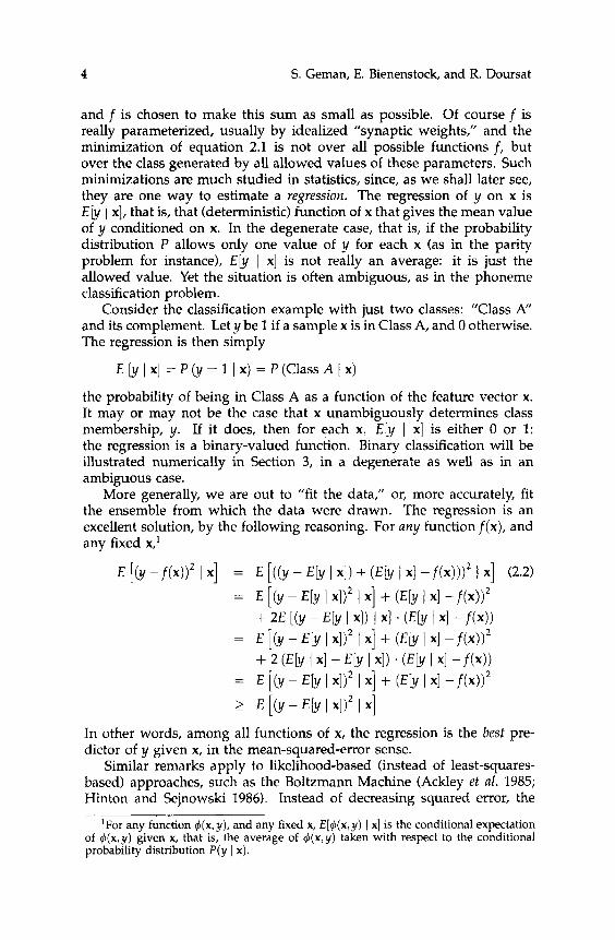
and f is chosen to make this sum as small as possible. Of course f is really parameterized, usually by idealized “synaptic weights,” and the minimization of equation 2.1 is not over all possible functions f, but over the class generated by all allowed values of these parameters. Such minimizations are much studied in statistics, since, as we shall later see, they are one way to estimate a regression. The regression of y on x is E[y I XI, that is, that (deterministic) function of x that gives the mean value of y conditioned on x. In the degenerate case, that is, if the probability distribution P allows only one value of y for each x (as in the parity problem for instance), E[y I x] is not really an average: it is just the allowed value. Yet the situation is often ambiguous, as in the phoneme classification problem.
Consider the classification example with just two classes: “Class A“ and its complement. Let y be 1 if a sample x is in Class A, and 0 otherwise. The regression is then simply
E [y I x] = P (y = 1 I x) = P (Class A I x)
the probability of being in Class A as a function of the feature vector x. It may or may not be the case that x unambiguously determines class membership, y. If it does, then for each x, Ely I x] is either 0 or 1: the regression is a binary-valued function. Binary classification will be illustrated numerically in Section 3, in a degenerate as well as in an ambiguous case.
More generally, we are out to “fit the data,” or, more accurately, fit the ensemble from which the data were drawn. The regression is an excellent solution, by the following reasoning. For any function f(x), and any fixed x,’
E [(Y - fW2 1x1 = E [((Y - Ek I XI) + ( E b I XI -f(X)))2 I XI (2.2)
= E [(Y - ElY I I x] + (El!/ I XI - f (x)) ’
= E [ (Y - El!/ I I x] + (ELy I XI - fW2
= E [(Y - E b I XI)* I x] + (Eb I XI -f(x))’
2 E [(Y - ELy I xu2 I x]
+ 2E [(Y - E k I XI) I xl . (Eb I XI - f (x ) )
+ 2 Fly I XI - E b I XI) . ( E [ y I XI - f (x))
In other words, among all functions of x, the regression is the best pre- dictor of y given x, in the mean-squared-error sense.
Similar remarks apply to likelihood-based (instead of least-squares- based) approaches, such as the Boltzmann Machine (Ackley et al. 1985; Hinton and Sejnowski 1986). Instead of decreasing squared error, the
‘For any function 4(x,y), and any fixed x, E[$(x,y) I x] is the conditional expectation of 4(x,y) given x, that is, the average of d(x,y) taken with respect to the conditional probability distribution P(y I x).

Neural Networks and the Bias/Variance Dilemma 5
Boltzmann Machine implements a Monte Carlo computational algorithm for increasing likelihood. This leads to the maximum-likelihood estima- tor of a probability distribution, at least if we disregard local maxima and other confounding computational issues. The maximum-likelihood estimator of a distribution is certainly well studied in statistics, primarily because of its many optimality properties. Of course, there are many other examples of neural networks that realize well-defined statistical estimators (see Section 5.1).
The most extensively studied neural network in recent years is prob- ably the backpropagation network, that is, a multilayer feedforward net- work with the associated error-backpropagation algorithm for minimiz- ing the observed sum of squared errors (Rumelhart et al. 1986a,b). With this in mind, we will focus our discussion by addressing least-squares estimators almost exclusively. But the issues that we will raise are ubiq- uitous in the theory of estimation, and our main conclusions apply to a broader class of neural networks.
2.2 Nonparametric Estimation and Consistency. If the response vari- able is binary, y E {O,l}, and if y = 1 indicates membership in "Class A," then the regression is just P(C1ass A I x ) , as we have already ob- served. A decision rule, such as "choose Class A if P(C1ass A I x ) > 1/2," then generates a partition of the range of x (call this range H ) into H A = { x : P(C1ass A I x) > 1/2} and its complement H - HA = HA. Thus, x E HA is classified as "A," x E H A is classified as "not A." It may be the case that HA and H A are separated by a regular surface (or "deci- sion boundary"), planar or quadratic for example, or the separation may be highly irregular.
Given a sequence of observations ( x l , y l ) , (x2, y2), . . . we can proceed to estimate P(C1ass A I x ) (= E[y I X I ) , and hence the decision bound- ary, from two rather different philosophies. On the one hand we can assume a priori that H A is known up to a finite, and preferably small, number of parameters, as would be the case if H A and HA were linearly or quadratically separated, or, on the other hand, we can forgo such as- sumptions and "let the data speak for itself." The chief advantage of the former, parametric, approach is of course efficiency: if the separation re- ally is planar or quadratic, then many fewer data are needed for accurate estimation than if we were to proceed without parametric specifications. But if the true separation departs substantially from the assumed form, then the parametric approach is destined to converge to an incorrect, and hence suboptimal solution, typically (but depending on details of the estimation algorithm) to a "best" approximation within the allowed class of decision boundaries. The latter, nonparamefric, approach makes no such a priori commitments.
The asymptotic (large sample) convergence of an estimator to the ob- ject of estimation is called consistency. Most nonparametric regression

6 S. Geman, E. Bienenstock, and R. Doursat
algorithms are consistent, for essentially any regression function E[y I XI.' This is indeed a reassuring property, but it comes with a high price: de- pending on the particular algorithm and the particular regression, non- parametric methods can be extremely slow to converge. That is, they may require very large numbers of examples to make relatively crude approx- imations of the target regression function. Indeed, with small samples the estimator may be too dependent on the particular samples observed, that is, on the particular realizations of (x, y) (we say that the variance of the estimator is high). Thus, for a fixed and finite training set, a paramet- ric estimator may actually outperform a nonparametric estimator, even when the true regression is outside of the parameterized class. These issues of bias and variance will be further discussed in Section 3.
For now, the important point is that there exist many consistent non- parametric estimators, for regressions as well as probability distributions. This means that, given enough training samples, optimal decision rules can be arbitrarily well approximated. These estimators are extensively studied in the modern statistics literature. Parzen windows and nearest- neighbor rules (see, e.g., Duda and Hart 1973; Hardle 1990), regular- ization methods (see, e.g., Wahba 1982) and the closely related method of sieves (Grenander 1981; Geman and Hwang 1982), projection pur- suit (Friedman and Stuetzle 1981; Huber 19851, recursive partitioning methods such as "CART," which stands for "Classification and Regres- sion Trees" (Breiman et al. 1984), Alternating Conditional Expectations, or "ACE" (Breiman and Friedman 1985), and Multivariate Adaptive Regres- sion Splines, or "MARS" (Friedman 1991), as well as feedforward neural networks (Rumelhart et al. 1986a,b) and Boltzmann Machines (Ackley et al. 1985; Hinton and Sejnowski 1986), are a few examples of techniques that can be used to construct consistent nonparametric estimators.
2.3 Some Applications of Nonparametric Inference. In this paper, we shall be mostly concerned with limitations of nonparametric methods, and with the relevance of these limitations to neural network models. But there is also much practical promise in these methods, and there have been some important successes.
An interesting and difficult problem in industrial "process specifica- tion" was recently solved at the General Motors Research Labs (Lorenzen 1988) with the help of the already mentioned CART method (Breiman et al. 1984). The essence of CART is the following. Suppose that there are m classes, y E (1.2,. . . , m}, and an input, or feature, vector x. Based on a training sample (XI, yl), . . . , (xN,yN) the CART algorithm constructs a partitioning of the (usually high-dimensional) domain of x into rectan-
*One has to specify the mode of convergence: the estimator is itself a function, and furthermore depends on the realization of a random training set (see Section 4.2). One also has to require certain technical conditions, such as measurability of the regression function.

Neural Networks and the BiasNariance Dilemma 7
gular cells, and estimates the class-probabilities { P ( y = k) : k = 1, . . . , m } within each cell. Criteria are defined that promote cells in which the es- timated class probabilities are well-peaked around a single class, and at the same time discourage partitions into large numbers of cells, relative to N. CART provides a family of recursive partitioning algorithms for approximately optimizing a combination of these competing criteria.
The GM problem solved by CART concerned the casting of certain engine-block components. A new technology known as lost-foam casting promises to alleviate the high scrap rate associated with conventional casting methods. A Styrofoam ”model” of the desired part is made, and then surrounded by packed sand. Molten metal is poured onto the Styrofoam, which vaporizes and escapes through the sand. The metal then solidifies into a replica of the styrofoam model.
Many “process variables” enter into the procedure, involving the set- tings of various temperatures, pressures, and other parameters, as well as the detailed composition of the various materials, such as sand. Engi- neers identified 80 such variables that were expected to be of particular importance, and data were collected to study the relationship between these variables and the likelihood of success of the lost-foam casting procedure. (These variables are proprietary.) Straightforward data anal- ysis on a training set of 470 examples revealed no good “first-order” predictors of success of casts (a binary variable) among the 80 process variables. Figure 1 (from Lorenzen 1988) shows a histogram comparison for that variable that was judged to have the most visually disparate his- tograms among the 80 variables: the left histogram is from a population of scrapped casts, and the right is from a population of accepted casts. Evi- dently, this variable has no important prediction power in isolation from other variables. Other data analyses indicated similarly that no obvious low-order multiple relations could reliably predict success versus failure. Nevertheless, the CART procedure identified achievable regions in the space of process variables that reduced the scrap rate in this production facility by over 75%.
As might be expected, this success was achieved by a useful mix of the nonparametric algorithm, which in principal is fully automatic, and the statistician’s need to bring to bear the realities and limitations of the production process. In this regard, several important modifications were made to the standard CART algorithm. Nevertheless, the result is a striking affirmation of the potential utility of nonparametric methods.
There have been many success stories for nonparametric methods. An intriguing application of CART to medical diagnosis is reported in Goldman et al. (19821, and further examples with CART can be found in Breiman et al. (1984). The recent statistics and neural network literatures contain examples of the application of other nonparametric methods as well. A much-advertised neural network example is the evaluation of loan applications (cf. Collins et al. 1989). The basic problem is to clas- sify a loan candidate as acceptable or not acceptable based on 20 or so

8 S. Geman, E. Bienenstock, and R. Doursat
Figure 1: Left histogram: distribution of process variable for unsuccessful cast- ings. Right histogram: distribution of same process variable for successful castings. Among all 80 process variables, this variable was judged to have the most dissimilar success/failure histograms. (Lorenzen 1988)
variabIes summarizing an applicant’s financial status, These include, for example, measures of income and income stability, debt and other fi- nancial obligations, credit history, and possibly appraised values in the case of mortgages and other secured loans. A conventional parametric statistical approach is the so-called logit model (see, for example, Cox 1970), which posits a linear relationship between the logistic transforma- tion of the desired variable (here the probability of a successful return to the lender) and the relevant independent variables (defining financial s t a t u ~ ) . ~ Of course, a linear model may not be suitable, in which case the logit estimator would perform poorly; it would be too biased. On the other hand, very large training sets are available, and it makes good sense to try less parametric methods, such as the backpropagation algo- rithm, the nearest-neighbor algorithm, or the ”Multiple-Neural-Network Learning System” advocated for this problem by Collins et al. (1989).
3The logistic transformation of a probability p is log,[p/(l - p ) ] .

Neural Networks and the BiasNariance Dilemma 9
These examples will be further discussed in Section 5, where we shall draw a sharp contrast between these relatively easy tasks and problems arising in perception and in other areas of machine intelligence.
3 Bias and Variance
3.1 The BiasIVariance Decomposition of Mean-Squared Error. The regression problem is to construct a functionf(x) based on a ”training set” ( x ~ , y ~ ) , . . . , (XN,YN), for the purpose of approximating y at future obser- vations of x. This is sometimes called “generalization,” a term borrowed from psychology. To be explicit about the dependence off on the data V = {(XI, yl), . . . , (XN, YN)}, we will write f(x; V) instead of simply f(x). Given D, and given a particular x, a natural measure of the effectiveness off as a predictor of y is
the mean-squared error (where €[.I means expectation with respect to the probability distribution P, see Section 2). In our new notation em- phasizing the dependency of f on V (which is fixed for the moment), equation 2.2 reads
E [(Y - f ( x ; m 2 I X > D ] = E [(Y - E [ y I XI)’ I X > 4
+ (f(x; 2)) - E[y I XI)’
E[(y-Ely I x ] ) ~ I x, V] does not depend on the data, V, or on the estimator, f; it is simply the variance of y given x. Hence the squared distance to the regression function,
measures, in a natural way, the effectiveness off as a predictor of y. The mean-squared error off as an estimator of the regression E [ y I x] is
€27 [(f(x;D) - Ely I XI)’] (3.1)
where E D represents expectation with respect to the training set, V, that is, the average over the ensemble of possible V (for fixed sample size N).
It may be that for a particular training set, V, f(x;V) is an excellent approximation of Ely I x], hence a near-optimal predictor of y. At the same time, however, it may also be the case that f(x; D) is quite different for other realizations of D, and in general varies substantially with V, or it may be that the average (over all possible V) of f(x; V) is rather far from the regression E [ y I XI. These circumstances will contribute large values in 3.1, making f(x; V) an unreliable predictor of y. A useful way to assess

10 S. Geman, E. Bienenstock, and R. Doursat
these sources of estimation error is via the bias/ variance decomposition, which we derive in a way similar to 2.2 for any x,
E D [(fh 2)) - E l y I XI)’]
= E D [ ( ( f ( x ; D ) - E D V(x;DO)l) + ( E D [ f ( x ; D ) ] - E l y I X I ) ) ‘ ] = E D [ ( f ( x ; D ) - E D [f(x;D)I)’] + E D [ ( E D [ f ( x ; D ) ] - E[y I XI) ’ ]
+ ED [ ( f ( x ; 2)) - E D [ f ( ~ D ) ] ) ( E D [ f ( ~ D)] - E[y I X I ) ] = E D [ ( f ( x ; D) - E D [ f ( ~ D ) ] )’I + ( E D V ( X ; D)] - E [ y I XI)’
+ ED [ f ( x ; D ) - E D [ f ( x ; D ) ] ] . ( E D [f(x;D)] - E[y I x ] ) = ( E D [ f ( x ; D ) ] - E l y I ~ 1 ) ~ “bias”
”variance” + E~ [ ~ ( x ; D) - E= ~ ( x ; D)] )’I If, on the average, f ( x ; D) is different from E[y I x], then f ( x ; D) is said to be biased as an estimator of E[y I X I . In general, this depends on P; the same f may be biased in some cases and unbiased in others.
As said above, an unbiased estimator may still have a large mean- squared error if the variance is large: even with EDV(X;D)] = E l y I x], f ( x ; D ) may be highly sensitive to the data, and, typically, far from the regression E l y I X I . Thus either bias or variance can contribute to poor performance.
There is often a tradeoff between the bias and variance contributions to the estimation error, which makes for a kind of “uncertainty principle” (Grenander 1951 ). Typically, variance is reduced through “smoothing,” via a combining, for example, of the influences of samples that are nearby in the input ( x ) space. This, however, will introduce bias, as details of the regression function will be lost; for example, sharp peaks and valleys will be blurred.
3.2 Examples. The issue of balancing bias and variance is much stud- ied in estimation theory. The tradeoff is already well illustrated in the one-dimensional regression problem: x = x E [0,1]. In an elementary version of this problem, y is related to x by
(3.2)
where g is an unknown function, and 77 is.zero-mean “noise” with distri- bution independent of x. The regression is then g ( x ) , and this is the best (mean-squared-error) predictor of y. To make our points more clearly, we will suppose, for this example, that only y is random - x can be chosen as we please. If we are to collect N observations, then a natural ”design” for the inputs is xi = i/N, 1 5 i 5 N, and the data are then the corresponding N values of y, 2, = {yl, . . . , yN}. An example (from Wahba and Wold 19751, with N = 100, g(x) = 4.26(ecX - 4e-& + 3ec3’), and 77 gaussian with standard deviation 0.2, is shown in Figure 2. The squares are the data points, and the broken curve, in each panel, is the
Y = g ( x ) + 77

Neural Networks and the Bias/Variance DiIemma 11
a
t
C
b
Figure 2: One hundred observations (squares) generated according to equation 4, with g ( x ) = 4.26(eCX - 4eCZX + 3 ~ ~ ~ ) . The noise is zero-mean gaussian with standard error 0.2. In each panel, the broken curve is g and the solid curve is a spline fit. (a) Smoothing parameter chosen to control variance. (b) Smoothing parameter chosen to control bias. (c) A compromising value of the smoothing parameter, chosen automatically by cross-validation. (From Wahba and Wold 1975)
regression, g(X) . (The solid curves are estimates of the regression, as will be explained shortly.)
The object is to make a guess at g(x), using the noisy observations, yi = g(xi) + yi, 1 5 i 5 N. At one extreme, f ( x ; D ) could be defined as the linear (or some other) interpolant of the data. This estimator is truly unbiased at x = xi, 1 5 i 5 N, since
E D v ( X i ; D)] == E [g(Xi) + ~ i ] g ( X i ) = E [y I xi]
Furthermore, if g is continuous there is also very little bias in the vicinity of the observation points, X i , 1 5 i 5 N. But if the variance of y is large, then there will be a large variance component to the mean-squared error (3.11, since
ED [V(xi;D) - ED v ( x i ; ~ ) 1 ) ~ ] = E D [k(xi) + vi - g(xi))’] = E

12 S. Geman, E. Bienenstock, and R. Doursat
which, since qi has zero mean, is the variance of 77,. This estimator is indeed very sensitive to the data.
At the other extreme, we may take f (x;V) = k ( x ) for some well- chosen function h(x), independent of V . This certainly solves the variance problem! Needless to say, there is likely to be a substantial bias, for this estimator does not pay any attention to the data.
A better choice would be an intermediate one, balancing some reason- able prior expectation, such as smoothness, with faithfulness to the ob- served data. One example is a feedforward neural network trained by er- ror backpropagation. The output of such a network isf(x; w) = f [ x ; w(V)], where w(D) is a collection of weights determined by (approximately) minimizing the sum of squared errors:
(3.3)
How big a network should we employ? A small network, with say one hidden unit, is likely to be biased, since the repertoire of available functions spanned by f ( x ; w) over allowable weights will in this case be quite limited. If the true regression is poorly approximated within this class, there will necessarily be a substantial bias. On the other hand, if we overparameterize, via a large number of hidden units and associated weights, then the bias will be reduced (indeed, with enough weights and hidden units, the network will interpolate the data), but there is then the danger of a significant variance contribution to the mean-squared error. (This may actually be mitigated by incomplete convergence of the minimization algorithm, as we shall see in Section 3.5.5.)
Many other solutions have been invented, for this simple regression problem as well as its extensions to multivariate settings (y -+ y E Rd, x + x E R‘, for some d > 1 and I > 1). Often splines are used, for example. These arise by first restricting f via a “smoothing criterion” such as
for some fixed integer m 2 1 and fixed A. (Partial and mixed partial derivatives enter when x + x E R’; see, for example, Wahba 1979.) One then solves for the minimum of
among all f satisfying equation 3.4. This minimization turns out to be tractable and yields f ( x ) = f ( x ; D ) , a concatenation of polynomials of degree 2m-1 on the intervals (xi, xi+l); the derivatives of the polynomials, up to order 2m -2, match at the “knots” {xi}El. With m = 1, for example, the solution is continuous and piecewise linear, with discontinuities in

Neural Networks and the BiasNariance Dilemma 13
the derivative at the knots. When m = 2 the polynomials are cubic, the first two derivatives are continuous at the knots, and the curve appears globally “smooth.” Poggio and Girosi (1990) have shown how splines and related estimators can be computed with multilayer networks.
The “regularization” or ”smoothing” parameter X plays a role simi- lar to the number of weights in a feedforward neural network. Small X produce small-variance high-bias estimators; the data are essentially ignored in favor of the constraint (“oversmoothing”). Large values of X produce interpolating splines: f ( x ; ; 2)) = y,, 1 5 i 5 N, which, as we have seen, may be subject to high variance. Examples of both oversmoothing and undersmoothing are shown in Figure 2a and b, respectively. The solid lines are cubic-spline (rn = 2) estimators of the regression. There are many recipes for choosing A, and other smoothing parameters, from the dnfa, a procedure known as ”automatic smoothing” (see Section 4.1). A popular example is called cross-validation (again, see Section 4,1), a version of which was used in Figure 2c.
There are of course many other approaches to the regression problem. Two in particular are the nearest-neighbor estimators and the kernel esti- mators, which we have used in some experiments both on artificial data and on handwritten numeral recognition. The results of these experi- ments will be reviewed in Section 3.5.
3.3 Nonparametric Estimation. Nonparametric regression estimators are characterized by their being consistent for all regression problems. Consistency requires a somewhat arbitrary specification: in what sense does the estimator f(x;V) converge to the regression E [ y I XI? Let us be explicit about the dependence off on sample size, N, by writing V = V N and then f ( x ; D ~ ) for the estimator, given the N observations DN. One version of consistency is ”pointwise mean-squared error”:
for each x. A more gIobal specification is in terms of integrated mean- squared error:
(3.5)
There are many variations, involving, for example, almost sure conver- gence, instead of the mean convergence that is defined by the expectation operator E D . Regardless of the details, any reasonable specification will require that both bias and variance go to zero as the size of the train- ing sample increases. In particular, the class of possible functions f(x; VN) must approach Ely I x] in some suitable sense? or there will necessarily
4The appropriate metric is the one used to define consistency. Lz , for example, with 3.5.

14 S. Geman, E. Bienenstock, and R. Doursat
be some residual bias. This class of functions will therefore, in general, have to grow with N. For feedforward neural networks, the possible functions are those spanned by all allowed weight values. For any fixed architecture there will be regressions outside of the class, and hence the network cannot realize a consistent nonparametric algorithm. By the same token, the spline estimator is not consistent (in any of the usual senses) whenever the regression satisfies
since the estimator itself is constrained to violate this condition (see equa- tion 3.4).
It is by now well-known (see, e.g., White 1990) that a feedforward neu- ral network (with some mild conditions on Ely I x] and network structure, and some optimistic assumptions about minimizing 3.3) can be made consistent by suitably letting the network size grow with the size of the training set, in other words by gradually diminishing bias. Analogously, splines are made consistent by taking X = AN T 03 sufficiently slowly. This is indeed the general recipe for obtaining consistency in nonparametric estimation: slowly remove bias. This procedure is somewhat delicate, since the variance must also go to zero, which dictates a gradual reduc- tion of bias (see discussion below, Section 5.1). The main mathematical issue concerns this control of the variance, and it is here that tools such as the Vapnikxervonenkis dimension come into play. We will be more specific in our brief introduction to the mathematics of consistency below (Section 4.2).
As the examples illustrate, the distinction between parametric and nonparametric methods is somewhat artificial, especially with regards to fixed and finite training sets. Indeed, most nonparametric estimators, such as feedforward neural networks, are in fact a sequence of parametric estimators indexed by sample size.
3.4 The Dilemma. Much of the excitement about artificial neural net- works revolves around the promise to avoid the tedious, difficult, and generally expensive process of articulating heuristics and rules for ma- chines that are to perform nontrivial perceptual and cognitive tasks, such as for vision systems and expert systems. We would naturally prefer to "teach our machines by example, and would hope that a good learning algorithm would "discover" the various heuristics and rules that apply to the task at hand. It would appear, then, that consistency is relevant: a consistent learning algorithm will, in fact, approach optimal performance, whatever the task. Such a system might be said to be unbiased, as it is not a priori dedicated to a particular solution or class of solutions. But the price to pay for achieving low bias is high variance. A ma- chine sufficiently versatile to reasonably approximate a broad range of
Neural Networks and the BiasNariance Dilemma 15
input/ output mappings is necessarily sensitive to the idiosyncrasies of the particular data used for its training, and therefore requires a very large training set. Simply put, dedicated machines are harder to build but easier to train.
Of course there is a quantitative tradeoff, and one can argue that for many problems acceptable performance is achievable from a more or less tabula rasa architecture, and without unrealistic numbers of training ex- amples. Or that specific problems may suggest easy and natural specific structures, which introduce the "right" biases for the problem at hand, and thereby mitigate the issue of sample size. We will discuss these matters further in Section 5.
3.5 Experiments in Nonparametric Estimation. In this section, we shall report on two kinds of experiments, both concerning classification, but some using artificial data and others using handwritten numerals. The experiments with artificial data are illustrative since they involve only two dimensions, making it possible to display estimated regres- sions as well as bias and variance contributions to mean-squared error. Experiments were performed with nearest-neighbor and Parzen-window estimators, and with feedforward neural networks trained via error back- propagation. Results are reported following brief discussions of each of these estimation methods.
3.5.1 Nearest-Neighbor Regression. This simple and time-honored ap- proach provides a good performance benchmark. The "memory" of the machine is exactly the training set V = {(xI,yI), , . . , (XN, y ~ ) ) . For any input vector x, a response vector y is derived from the training set by av- eraging the responses to those inputs from the training set which happen to lie close to x. Actually, there is here a collection of algorithms indexed by an integer, "k," which determines the number of neighbors of x that enter into the average. Thus, the k-nearest-neighbor estimator is just
where Nk(x) is the collection of indices of the k nearest neighbors to x among the input vectors in the training set {xi}:,. (There is also a k-nearest-neighbor procedure for classification: If y = y E { 1,2, . . . , C}, representing C classes, then we assign to x the class y E { 1,2, . . . , C) most frequent among the set { ~ i } i ~ N ~ ( ~ ) , where y i is the class of the training input xi.)
If k is "large" (e.g., k is almost N) then the response f(x; V) is a rela- tively smooth function of x, but has little to do with the actual positions of the x[s in the training set. In fact, when k = N , f(x;D) is indepen- dent of x, and of {xi}El; the output is just the average observed output 1 / N ELl yi. When N is large, 1 /N ELl yi is likely to be nearly unchanged

16 S. Geman, E. Bienenstock, and R. Doursat
from one training set to another. Evidently, the variance contribution to mean-squared error is then small. On the other hand, the response to a particular x is systematically biased toward the population response, regardless of any evidence for local variation in the neighborhood of x. For most problems, this is of course a bad estimation policy.
The other extreme is the first-nearest-neighbor estimator; we can ex- pect less bias. Indeed, under reasonable conditions, the bias of the first- nearest-neighbor estimator goes to zero as N goes to infinity. On the other hand, the response at each x is rather sensitive to the idiosyncrasies of the particular training examples in D. Thus the variance contribution to mean-squared error is typically large.
From these considerations it is perhaps not surprising that the best solution in many cases is a compromise between the two extremes k = 1 and k = N. By choosing an intermediate k, thereby implementing a reasonable amount of smoothing, one may hope to achieve a significant reduction of the variance, without introducing too much bias. If we now consider the case N + 00, the k-nearest-neighbor estimator can be made consistent by choosing k = k~ T 00 sufficiently slowly. The idea is that the variance is controlled (forced to zero) by k~ T m, whereas the bias is controlled by ensuring that the kNth nearest neighbor of x is actually getting closer to x as N -+ m.
3.5.2 Parzen- Window Regression. The "memory" of the machine is again the entire training set D, but estimation is now done by combin- ing "kernels," or "Parzen windows," placed around each observed input point xi, 1 5 i 5 N. The form of the kernel is somewhat arbitrary, but it is usually chosen to be a nonnegative function of x that is maximum at x = 0 and decreasing away from x = 0. A common choice is
the gaussian kernel, for x E Rd. The scale of the kernel is adjusted by a "bandwidth CJ: W ( x ) -+ (1/0)~W(x/o) . The effect is to govern the extent to which the window is concentrated at x = 0 (small CJ), or is spread out over a significant region around x = 0 (large (T). Having fixed a kernel W(.), and a bandwidth CJ, the Parzen regression estimator at x is formed from a weighted average of the observed responses {yi}El:
Clearly, observations with inputs closer to x are weighted more heavily. There is a close connection between nearest-neighbor and Parzen-
window estimation. In fact, when the bandwidth o is small, only close neighbors of x contribute to the response at this point, and the procedure is akin to k-nearest-neighbor methods with small k. On the other hand,

Neural Networks and the Bias/Variance Dilemma 17
when o is large, many neighbors contribute significantly to the response, a situation analogous to the use of large values of k in the k-nearest- neighbor method. In this way, D governs bias and variance much as k does for the nearest-neighbor procedure: small bandwidths generally offer high-variance/low-bias estimation, whereas large bandwidths incur relatively high bias but low variance.
There is also a Parzen-window procedure for classification: we assign to x the class y = y E {1,2, . . . ~ C} which maximizes
where Ny is the number of times that the classification y is seen in the training set, N,, = #{i : yi = y}. If W ( x ) is normalized, so as to integrate to one, then fu(x; 23) estimates the density of inputs associated with the class y (known as the ”class-conditional density”). Choosing the class with maximum density at x results in minimizing the probability of error, at least when the classes are a priori equally likely. (If the a priori probabili- ties of the C classes, p(y) y E (1.2, . . . , C}, are unequal, but known, then the minimum probability of error is obtained by choosing y to maximize P(Y) . fy (x ;W
3.5.3 Feedforward Network Trained by Error Backpropagation. Most read- ers are already familiar with this estimation technique. We used two- layer networks, that is, networks with one hidden layer, with full con- nections between layers. The number of inputs and outputs depended on the experiment and on a coding convention; it will be laid out with the results of the different experiments in the ensuing paragraphs. In the usual manner, all hidden and output units receive one special input that is nonzero and constant, allowing each unit to learn a “threshold.”
Each unit outputs a value determined by the sigmoid function
(3.8)
given the input
Here, {<,} represents inputs from the previous layer (together with the above-mentioned constant input) and {w,} represents the weights (”syn- aptic strengths”) for this unit. Learning is by discrete gradient descent, using the full training set at each step. Thus, if w(t) is the ensemble of all weights after t iterations, then
w(t + 1 ) = w(t) - FV,&[W(t)] (3.9)

18 S. Geman, E. Bienenstock, and R. Doursat
where t is a control parameter, V, is the gradient operator, and E(w) is the mean-squared error over the training samples. Specifically, if f(x; w) denotes the (possibly vector-valued) output of the feed forward network given the weights w, then
where, as usual, the training set is 2, = ((XI, yl), . . . , (XN, y ~ ) } . The gra- dient, V,E(w), is calculated by error backpropagation (see Rumelhart et al. 1986a,b). The particular choices of F and the initial state w(0), as well as the number of iterations of 3.9, will be specified during the discussion of the experimental results.
It is certainly reasonable to anticipate that the number of hidden units would be an important variable in controlling the bias and variance con- tributions to mean-squared error. The addition of hidden units con- tributes complexity and presumably versatility, and the expected price is higher variance. This tradeoff is, in fact, observed in experiments reported by several authors (see, for example, Chauvin 1990; Morgan and Bourlard 1990), as well as in our experiments with artificial data (Section 3.5.4). However, as we shall see in Section 3.5.5, a somewhat more complex picture emerges from our experiments with handwritten numerals (see also Martin and Pittman 1991).
3.5.4 Experiments with Artificial Data. The desired output indicates one of two classes, represented by the values f .9 . [This coding was used in all three methods, to accommodate the feedforward neural network, in which the sigmoid output function equation 3.8 has asymptotes at i l . By coding classes with values 50.9, the training data could be fit by the network without resorting to infinite weights.] In some of the ex- periments, the classification is unambiguously determined by the input, whereas in others there is some "overlap" between the two classes. In either case, the input has two components, x = (x1,x*), and is drawn from the rectangle [-6,6] x [-1.5,1.5].
In the unambiguous case, the classification is determined by the curve x2 = sin(txl), which divides the rectangle into "top" [x2 >_ sin((n/2)x~), y = 0.91 and "bottom" [xq < sin((7r/2)xl),y = -0.91 pieces. The regression is then the binary-valued function E[y 1 x] = .9 above the sinusoid and -0.9 below (see Fig. 3a). The training set, 2, = {(x,,yl), .. . , (xN,YN)}, is constructed to have 50 examples from each class. For y = 0.9, the 50 inputs are chosen from the uniform distribution on the region above the sinusoid; the y = -0.9 inputs are chosen uniformly from the region below the sinusoid.
Classification can be made ambiguous within the same basic setup, by randomly perturbing the input vector before determining its class. To describe precisely the random mechanism, let us denote by B1 (x) the

Neural Networks and the Bias/Variance Dilemma 19
a
b
Figure 3: Two regression surfaces for experiments with artificial data. (a) Output is deterministic function of input, f0.9 above sinusoid, and -0.9 below sinusoid. (b) Output is perturbed randomly. Mean value of zero is coded with white, mean value of $0.9 is coded with gray, and mean value of -0.9 is coded with black.
disk of unit radius centered at x. For a given x, the classification y is chosen randomly as follows: x is "perturbed" by choosing a point z from the uniform distribution on Bl(x), and y is then assigned value 0.9 if z2 2 sin((7r/2)zl), and -0.9 otherwise. The resulting regression, E[y I XI], is depicted in Figure 3b, where white codes the value zero, gray codes the value f0.9, and black codes the value -0.9. Other values are coded by interpolation. (This color code has some ambiguity to it: a given gray level does not uniquely determine a value between -0.9 and 0.9. This code was chosen to emphasize the transition region, where y x 0.) The effect of the classification ambiguity is, of course, most pronounced near the "boundary" x2 = sin((7r/Z)xI).
If the goal is to minimize mean-squared error, then the best response to a given x is E [ y I XI. On the other hand, the minimum error classifier will assign class "$0.9" or "-0.9" to a given x, depending on whether E [ y I x] 2 0 or not: this is the decision function that minimizes the probability of misclassifying x. The decision boundary of the optimal classifier ({x : E [ y I x] = 0)) is very nearly the original sinusoid x2 = sin((a/2)xl); it is depicted by the whitest values in Figure 3b.
The training set for the ambiguous classification task was also con- structed to have 50 examples from each class. This was done by repeated Monte Carlo choice of pairs (x,y), with x chosen uniformly from the rect- angle [-6,6] x [-1.5,1.5] and y chosen by the above-described random

20 S. Geman, E. Bienenstock, and R. Doursat
mechanism. The first 50 examples for which y = 0.9 and the first 50 examples for which y = -0.9 constituted the training set.
In each experiment, bias, variance, and mean-squared error were eval- uated by a simple Monte Carlo procedure, which we now describe. De- note by f(x;V) the regression estimator for any given training set V. Recall that the (squared) bias, at x, is just
(E.DV(x; .O)l - Ely I xll2 and that the variance is
ED [(f(x;V) - E D ~ ( X ; ~ ) ] ) ~ ]
These were assessed by choosing, independently, 100 training sets V', .O2# . . ., Dl00 , and by forming the corresponding estimators f(x; Dl), . . . , f(x;D,'"). Denote by f(x) the average response at x: f(x) = ( l / l O O ) EkEl f(x;@). Bias and variance were estimated via the formulas:
Bias(x) = (f(x) - Ely I XI)'
(Recall that E[y I x] is known exactly - see Fig. 3.) The sum, Bias(x) + Variance(x) is the (estimated) mean-squared error, and is equal to
In several examples we display Bias(x) and Variance(x) via gray-level pictures on the domain [-6,6] x [-1.5,1.5]. We also report on integrated bias, variance, and mean-squared error, obtained by simply integrating these functions over the rectangular domain of x (with respect to the uniform distribution).
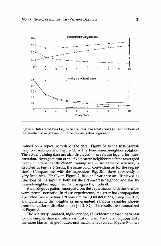
The experiments with artificial data included both nearest-neighbor estimation and estimation by a feedforward neural network. Results of the experiments with the nearest-neighbor procedure are summarized in Figure 4.
In both the deterministic and the ambiguous case, bias increased while variance decreased with the number of neighbors, as should be expected from our earlier discussion. In the deterministic case, the least mean- squared error is achieved using a small number of neighbors, two or three; there is apparently, and perhaps not surprisingly, little need to control the variance. In contrast, the more biased eight- or nine-nearest- neighbor estimator is best for the ambiguous task.
Figures 5 through 7 demonstrate various additional features of the results from experiments with the ambiguous classification problem. Fig- ure 5 shows the actual output, to each possible input, of two machines
Neural Networks and the Bias/Variance Dilemma 21
Deterministic Classification 0.4, I
I 1 2 3 4 5 6 I 8 9 10
0.5
0.4
0.3
0.2
0.1
0 1 2 3 4 5 6 I 8 9 10
# Neighbors
Figure 4: Integrated bias (os), variance (xs), and total error (+s) as functions of the number of neighbors in the nearest-neighbor regression.
trained on a typical sample of the data: Figure 5a is the first-nearest- neighbor solution and Figure 5b is the two-nearest-neighbor solution. The actual training data are also displayed - see figure legend for inter- pretation. Average output of the five-nearest-neighbor machine (averaged over 100 independently chosen training sets - see earlier discussion) is depicted in Figure 6 (using the same color convention as for the regres- sion). Compare this with the regression (Fig. 3b): there apparently is very little bias. Finally, in Figure 7, bias and variance are displayed as functions of the input x, both for the first-nearest-neighbor and the 10- nearest-neighbor machines. Notice again the tradeoff.
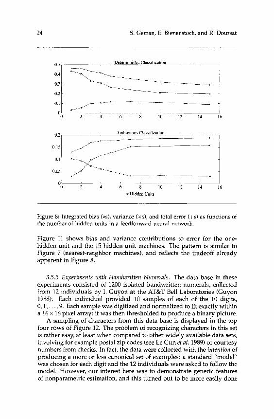
An analogous pattern emerged from the experiments with the feedfor- ward neural network. In these experiments, the error-backpropagation algorithm (see equation 3.9) was run for 3,000 iterations, using t = 0.05, and initializing the weights as independent random variables chosen from the uniform distribution on [-0.2,0.2]. The results are summarized in Figure 8.
The relatively unbiased, high-variance, 15-hidden-unit machine is best for the simpler deterministic classification task. For the ambiguous task, the more biased, single-hidden-unit machine is favored. Figure 9 shows

22 S. Geman, E. Bienenstock, and R. Doursat
Figure 5: Nearest-neighbor estimates of regression surface shown in Figure 3b. Gray-level code is the same as in Figure 3. The training set comprised 50 examples with values +0.9 (circles with white centers) and 50 examples with values -0.9 (circles with black centers). (a) First-nearest-neighbor estimator. (b) Two-nearest-neighbor estimator.
Figure 6: Average output of 100 five-nearest-neighbor machines, trained on independent data sets. Compare with the regression surface shown in Figure 3b (gray-level code is the same) - there is little bias.
the output of two typical machines, with five hidden units each. Both were trained for the ambiguous classification task, but using statisti- cally independent training sets. The contribution of each hidden unit is partially revealed by plotting the line ~ 1 x 1 t ~ 2 x 2 + w3 = 0, where x = (xI,x2) is the input vector, w1 and w2 are the associated weights, and w3 is the threshold. On either side of this line, the unit’s output is a function solely of distance to the line. The differences between these two machines hint at the variance contribution to mean-squared error (roughly 0.13 - see Fig. 8). For the same task and number of hidden
Neural Networks and the Bias/Variance Dilemma 23
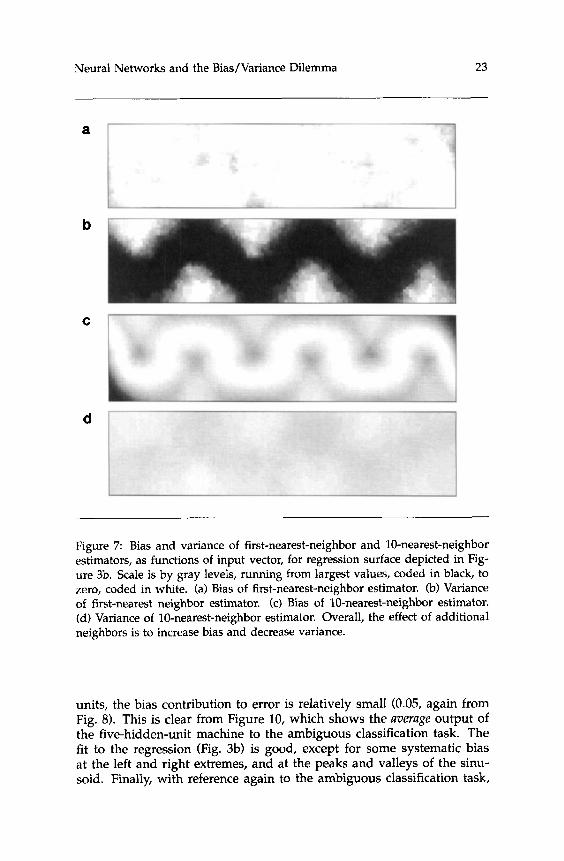
Figure 7: Bias and variance of first-nearest-neighbor and 10-nearest-neighbor estimators, as functions of input vector, for regression surface depicted in Fig- ure 3b. Scale is by gray levels, running from largest values, coded in black, to zero, coded in white. (a) Bias of first-nearest-neighbor estimator. (b) Variance of first-nearest neighbor estimator. (c) Bias of 10-nearest-neighbor estimator. (d) Variance of 10-nearest-neighbor estimator. Overall, the effect of additional neighbors is to increase bias and decrease variance.
units, the bias contribution to error is relatively small (0.05, again from Fig. 8). This is clear from Figure 10, which shows the average output of the five-hidden-unit machine to the ambiguous classification task. The fit to the regression (Fig. 3b) is good, except for some systematic bias at the left and right extremes, and at the peaks and valleys of the sinu- soid. Finally, with reference again to the ambiguous classification task,
24 S. Geman, E. Bienenstock, and R. Doursat
Determini 0.5 I istic Classification
"0 2 4 6 n 10 12 14 16
Ambiguous Classification 0 2
---w x
0 2 4 6 8 10 12 14 16 # Hidden Units
0 0s
0 -
Figure 8: Integrated bias (os), variance (xs), and total error (+s) as functions of the number of hidden units in a feedforward neural network.
Figure 11 shows bias and variance contributions to error for the one- hidden-unit and the 15-hidden-unit machines. The pattern is similar to Figure 7 (nearest-neighbor machines), and reflects the tradeoff already apparent in Figure 8.
3.5.5 Experiments with Handwritten Numerals. The data base in these experiments consisted of 1200 isolated handwritten numerals, collected from 12 individuals by I. Guyon at the AT&T Bell Laboratories (Guyon 1988). Each individual provided 10 samples of each of the 10 digits, 0 ,1 , . . . ,9. Each sample was digitized and normalized to fit exactly within a 16 x 16 pixel array; it was then thresholded to produce a binary picture.
A sampling of characters from this data base is displayed in the top four rows of Figure 12. The problem of recognizing characters in this set is rather easy, at least when compared to other widely available data sets, involving for example postal zip codes (see Le Cun et al. 1989) or courtesy numbers from checks. In fact, the data were collected with the intention of producing a more or less canonical set of examples: a standard "model" was chosen for each digit and the 12 individuals were asked to follow the model. However, our interest here was to demonstrate generic features of nonparametric estimation, and this turned out to be more easily done
Neural Networks and the Bias/Variance Dilemma 25
Figure 9: Output of feedfonvard neural networks trained on two independent samples of size 100. Actual regression is depicted in Figure 3b, with the same gray-level code. The training set comprised 50 examples with values +0.9 (cir- cles with white centers) and 50 examples with values -0.9 (circles with black centers). Straight lines indicate points of zero output for each of the five hid- den units - outputs are functions of distance to these lines. Note the large variation between these machines. This indicates a high variance contribution to mean-squared error.
Figure 1 0 Average output of 100 feedforward neural networks with five hidden units each, trained on independent data sets. The regression surface is shown in Figure 3b, with the same gray-level code.
with a somewhat harder problem; we therefore replaced the digits by a new, “corrupted,” training set, derived by flipping each pixel (black to white or white to black), independently, with probability 0.2. See the bottom four rows of Figure 12 for some examples. Note that this corruption does not in any sense mimic the difficulties encountered in

26 S. Geman, E. Bienenstock, and R. Doursat
a
b
C
Figure 11: Bias and variance of single-hidden-unit and 15-hidden-unit feed- forward neural networks, as functions of input vector. Regression surface is depicted in Figure 3b. Scale is by gray levels, running from largest values, coded in black, to zero, coded in white. (a) Bias of single-hidden-unit machine. (b) Variance of single-hidden-unit machine. (c) Bias of 15-hidden-unit machine. (d) Variance of 15-hidden-unit machine. Bias decreases and variance increases with the addition of hidden units.
real problems of handwritten numeral recognition; the latter are linked to variability of shape, style, stroke widths, etc.
The input x is a binary 16 x 16 array. We perform no ”feature extrac- tion” or other preprocessing. The classification, or output, is coded via a 10-dimensional vector y = (yo,. . . , y~) , where yi = +0.9 indicates the digit ’5,” and yi = -0.9 indicates “not i.” Each example in the (noisy) data set is paired with the correct classification vector, which has one component with value +0.9 and nine components with values -0.9.

Neural Networks and the Bias/Variance Dilemma 27
Figure 12: Top four rows: examples of handwritten numerals. Bottom four rows: same examples, corrupted by 20% flip rate (black to white or white to black).
To assess bias and variance, we set aside half of the data set (600 digits), thereby excluding these examples from training. Let us de- note these excluded examples by (x601, y601), . . . , (xI~M), ~ I ~ o o ) , and the re- maining examples by (xl, yl), . . . , (x600,y6M)). The partition was such that each group contained 60 examples of each digit; it was otherwise ran- dom. Algorithms were trained on subsets of {(xl,yl)}fz, and assessed
Each training set V consisted of 200 examples, 20 of each digit, cho- sen randomly from the set {(xi,yi)}z:. As with the previous data set, performance statistics were collected by choosing independent training sets, V1, . . . , P, and forming the associated (vector-valued) estimators f(x; V'), . . ., f(x; p). The performances of the nearest-neighbor and Parzen-window methods were assessed by using M = 100 independent training sets. For the error-backpropagation procedure, which is much more computationally intensive, M = 50 training sets were generally used.
Let us again denote by f(x) the average response at x over all training sets. For the calculation of bias, this average is to be compared with the
on {(xi,Yi)};2%.

28 S. Geman, E. Bienenstock, and R. Doursat
regression E[y I XI. Unlike the previous example (“artificial data”), the regression in this case is not explicitly available. Consider, however, the 600 noisy digits in the excluded set: {x1};2’&. Even with 20% corrup- tion, the classification of these numerals is in most cases unambiguous, as judged from the bottom rows of Figure 12. Thus, although this is not quite what we called a “degenerate“ case in Section 2.1, we can approx- imate the regression at XI, 601 5 I 5 1200, to be the actual classification, y~ : E[y I XI] x yl. Of course there is no way to display visually bias and variance as functions of x, as we did with the previous data, but we can still calculate approximate integrated bias, variance, and mean-squared error, using the entire excluded set, XbOl, . . . , xl20o, and the associated (ap- proximate) “regressions” y60l . . . . , ~ 1 2 0 0 :
1 1200
Integrated Bias M ~ C 1f(xI) - yII2 ‘O0 f=601
1 1200 1 M
6oo /=60] k=l Integrated Mean-Squared Error = - C - C If(xr; Dk) - yl 12
The last estimate (for integrated mean-squared error) is exactly the sum of the first two (for integrated bias and integrated variance).
Notice that the nearest-neighbor and Parzen-window estimators are both predicated on the assignment of a distance in the input (x) space, which is here the space of 16 x 16 binary images, or, ignoring the lattice structure, simply (0. 1}256. We used Hamming distance for both esti- mators. (In Section 6 , we shall report on experiments using a different metric for this numeral recognition task.) The kernel for the Parzen- window experiments was the exponential: W ( x ) = exp{-lxl}, where 1x1 is the Hamming distance to the zero vector.
We. have already remarked on the close relation between the kernel and nearest-neighbor methods. It is, then, not surprising that the ex- perimental results for these two methods were similar in every regard. Figures 13 and 14 show the bias and variance contributions to error, as well as the total (mean-squared) error, as functions of the respective “smoothing parameters” - the number of nearest neighbors and the ker- nel ”bandwidth.” The bias/variance tradeoff is well illustrated in both figures.
As was already noted in Sections 3.5.1 and 3.5.2, either machine can be used as a classifier. In both cases, the decision rule is actually asymptot- ically equivalent to implementing the obvious decision function: choose that classification whose 10-component coding is closest to the machine‘s output. To help the reader calibrate the mean-squared-error scale in these figures, we note that the values 1 and 2 in mean-squared error corre- spond, roughly, to 20 and 40% error rates, respectively.

Neural Networks and the Bias/Variance Dilemma 29
1 TotalError A
Bias r :4, Variance
k
Figure 13: Nearest-neighbor regression for handwritten numeral recognition. Bias, variance, and total error as a function of number of neighbors.
The results of experiments with the backpropagation network are more complex. Indeed, the networks output to a given input x is not uniquely defined by the sole choice of the training set V and of a “smooth- ing parameter,” as it is in the nearest-neighbor or the Parzen-window case. As we shall now see, convergence issues are important, and may introduce considerable variation in the behavior of the network. In the following experiments, the learning algorithm (equation 3.9) was initial- ized with independent and uniformly distributed weights, chosen from the interval [-0.1,0.1]; the gain parameter, E, was 0.1.
Figure 15 shows bias, variance, and total error, for a four-hidden- unit network, as a function of iteration trial (on a logarithmic scale). We observe that minimum total error is achieved by stopping the training after about 100 iterations, despite the fact that the fit to the training data

30 S. Geman, E. Bienenstock, and R. Doursat
Variance
10 u) 25
Figure 14: Kernel regression for handwritten numeral recognition. Bias, vari- ance, and total error as a function of kernel bandwidth.
continues to improve, as depicted by the curve labeled “learning.“ Thus, even with just four hidden units, there is a danger of “overfitting,“ with consequent high variance. Notice indeed the steady decline in bias and increase in variance as a function of training time.
This phenomenon is strikingly similar to one observed in several other applications of nonparametric statistics, such as maximum-likelihood re- construction for emission tomography (cf. Vardi et al. 1985; Veklerov and Llacer 1987). In that application, the natural “cost functional” is the (neg- ative) log likelihood, rather than the observed mean-squared error. Some- what analogous to gradient descent is the “ E - M algorithm (Dempster et al. 1976, but see also Baum 1972) for iteratively increasing likelihood. The reconstruction is defined on a pixel grid whose resolution plays a role similar to the number of hidden units. For sufficiently fine grids,

Neural Networks and the Bias/Variance Dilemma 31
log(time)
Figure 15: Neural network with four hidden units trained by error backprop- agation. The curve marked “Learning” shows the mean-squared error, on the training set, as a function of the number of iterations of backpropagation [de- noted ”log(time)”]. The best machine (minimum total error) is obtained after about 100 iterations; performance degrades with further training.
the E-M algorithm produces progressively better reconstructions up to a point, and then decisively degrades.
In both applications there are many solutions that are essentially con- sistent with the data, and this, in itself, contributes importantly to vari- ance. A manifestation of the same phenomenon occurs in a simpler setting, when fitting data with a polynomial whose degree is higher than the number of points in the data set. Many different polynomials are consistent with the data, and the actual solution reached may depend critically on the algorithm used as well as on the initialization.
Returning to backpropagation, we consistently found in the experi-

32 S. Geman, E. Bienenstock, and R. Doursat
3
5 10 IS m # Hidden Units
Figure 16: Total error, bias, and variance of feedforward neural network as a function of the number of hidden units. Training is by error backpropagation. For a fixed number of hidden units, the number of iterations of the backprop- agation algorithm is chosen to minimize total error.
ments with handwritten numerals that better results could be achieved by stopping the gradient descent well short of convergence; see, for ex- ample, Chauvin (1990) and Morgan and Bourlard (1990) who report on similar findings. Keeping in mind these observations, we have plotted, in Figure 16, bias, variance, and total mean-squared error as a function of the number of hidden units, where for each number of hidden units we chose the optimal number of learning steps (in terms of minimizing total error). Each entry is the result of 50 trials, as explained previously, with the sole exception of the last experiment. In this experiment, in- volving 24 hidden units, only 10 trials were used, but there was very little fluctuation around the point depicting (averaged) total error.

Neural Networks and the Bias/Variance Dilemma 33
The basic trend is what we expect: bias falls and variance increases with the number of hidden units. The effects are not perfectly demon- strated (notice, for example, the dip in variance in the experiments with the largest numbers of hidden units), presumably because the phenome- non of overfitting is complicated by convergence issues and perhaps also by our decision to stop the training prematurely. The lowest achievable mean-squared error appears to be about 2.
4 Balancing Bias and Variance
This section is a brief overview of some techniques used for obtaining optimal nonparametric estimators. It divides naturally into two parts: the first deals with the finite-sample case, where the problem is to do one’s best with a given training set of fixed size; the second deals with the asymptotic infinite-sample case. Not surprisingly, the first part is a review of relatively informal “recipes,” whereas the second is essentially mathematical.
4.1 Automatic Smoothing. As we have seen in the previous section, nonparametric estimators are generally indexed by one or more parame- ters which control bias and variance; these parameters must be properly adjusted, as functions of sample size, to ensure consistency, that is, con- vergence of mean-squared error to zero in the large-sample-size limit. The number of neighbors k, the kernel bandwidth GT, and the number of hidden units play these roles, respectively, in nearest-neighbor, Parzen- window, and feedforward-neural-network estimators. These “smoothing parameters” typically enforce a degree of regularity (hence bias), thereby “controlling” the variance. As we shall see in Section 4.2, consistency the- Qrems specify asymptotic rates of growth or decay of these parameters to guarantee convergence to the unknown regression, or, more generally, to the object of estimation. Thus, for example, a rate of growth of the number of neighbors or of the number of hidden units, or a rate of decay of the bandwidth, is specified as a function of the sample size N .
Unfortunately, these results are of a strictly asymptotic nature, and generally provide little in the way of useful guidelines for smoothing- parameter selection when faced with a fixed and finite training set V. It is, however, usually the case that the performance of the estimator is sensitive to the degree of smoothing. This was demonstrated previ- ously in the estimation experiments, and it is a consistent observation of practitioners of nonparametric methods. This has led to a search for ”automatic” or “data-driven” smoothing: the selection of a smoothing parameter based on some function of the data itself.
The most widely studied approach to automatic smoothing is **cross- validation.” The idea of this technique, usually attributed to Stone (19741, is as follows. Given a training set VN = { (x~ ,y~ ) , . .. , (XN,YN)} and a

34 S . Geman, E. Bienenstock, and R. Doursat
"smoothing parameter" X, we denote, generically, an estimator by f(x;N, A, D N ) [see, for example, (3.6) with X = k or (3.7) with X = r r ] . Cross-validation is based on a "leave-one-out" assessment of estimation performance. Denote by V(')N, 1 5 i 2 N, the data set excluding the ith observation ( x , , y ; ) : D(')N = { ( x l , y l ) , . . . , ( x i - l , y i - l ) , ( x i + ! , y i + l ) , . . ., ( x N , Y N ) } . Now fix A and form the estimator f ( x ; N - 1, X , D ( ' ) N ) , which is independent of the excluded observation ( x ; , y i ) . We can "test," or "cross-validate," on the excluded data: if f ( x , ; N -- 1, A, D$)) is close to yi, then there is some evidence in favor of f (x ; N, A, D N ) as an estimator of E[y I XI, at least for large N, wherein we do not expect f ( x ; N - 1, A,Di ' ) and f(x; N, A, DN) to be very different. Better still is the pooled assessment
The cross-validated smoothing parameter is the minimizer of A( A), which we will denote by A*. The cross-validated estimator is thenf(x;N, A', DN) .
Cross-validation is computation-intensive. In the worst case, we need to form N estimators at each value of A, to generate A(A), and then to find a global minimum with respect to A. Actually, the computation can often be very much reduced by introducing closely related (sometimes even better) assessment functions, or by taking advantage of special structure in the particular function f ( x ; N, A, D N ) at hand. The reader is referred to Wahba (1984,1985) and OSullivan and Wahba (1985) for various gener- alizations of cross-validation, as well as for support of the method in the way of analytic arguments and experiments with numerous applications. In fact, there is now a large statistical literature on cross-validation and related methods (Scott and Terrell 1987; Hardle et al. 1988; Marron 1988; Faraway and Jhun 1990; Hardle 1990 are some recent examples), and there have been several papers in the neural network literature as well - see White (1988,19901, Hansen and Salamon (19901, and Morgan and Bourlard (1990).
Computational issues aside, the resulting estimator, f ( x ; N, A*, DN) , is often strikingly effective, although some "pathological" behaviors have been pointed out (see, tor example, Schuster and Gregory 1981). In gen- eral, theoretical underpinnings of cross-validation remain weak, at least as compared to the rather complete existing theory of consistency for the original (not cross-validated) estimators.
Other mechanisms have been introduced with the same basic design goal: prevent overfitting and the consequent high contribution of vari- ance to mean-squared error (see, for example, Mozer and Smolensky 1989 and Karnin 1990 for some "pruning" methods for neural networks). Most of these other methods fall into the Bayesian paradigm, or the closely re- lated method of regularization. In the Bayesian approach, likely regular- ities are specified analytically, and a priori. These are captured in a prior probability distribution, placed on a space of allowable input-to-output mappings ("machines"). It is reasonable to hope that estimators then

Neural Networks and the BiasNariance Dilemma 35
derived through a proper Bayesian analysis would be consistent; there should be no further need to control variance, since the smoothing, as it were, has been imposed a priori. Unfortunately, in the nonparametric case it is necessary to introduce a distribution on the infinite-dimensional space of allowable mappings, and this often involves serious analytical, not to mention computational, problems. In fact, analytical studies have led to somewhat surprising findings about consistency or the lack thereof (see Diaconis and Freedman 1986).
Regularization methods rely on a “penalty function,” which is added to the observed sum of squared errors and promotes (is minimum at) ”smooth,” or “parsimonious,” or otherwise “regular” mappings. Min- imization can then be performed over a broad, possibly even infinite- dimensional, class of machines; a properly chosen and properly scaled penalty function should prevent overfitting. Regularization is very sim- ilar to, and sometimes equivalent to, Bayesian estimation under a prior distribution that is essentially the exponential of the (negative) penalty function. There has been much said about choosing the ”right” penalty function, and attempts have been made to derive, logically, information- based measures of machine complexity from “first principles” (see Akaike 1973; Rissanen 1986). Regularization methods, complexity-based as well as otherwise, have been introduced for neural networks, and both an- alytical and experimental studies have been reported (see, for example, Barron 1991; Chauvin 1990).
4.2 Consistency and Vapnik-cervonenkis Dimensionality. The stu- dy of neural networks in recent years has involved increasingly sophis- ticated mathematics (cf. Barron and Barron 1988; Barron 1989; Baum and Haussler 1989; Haussler 1989b; White 1989, 1990; Amari 1990; Amari et al. 1990; Azencott 1990; Baum 1990a1, often directly connected with the statistical-inference issues discussed in the previous sections. In particu- lar, machinery developed for the analysis of nonparametric estimation in statistics has been heavily exploited (and sometimes improved on) for the study of certain neural network algorithms, especially least-squares al- gorithms for feedforward neural networks. A reader unfamiliar with the mathematical tools may find this more technical literature unapproach- able. He may, however, benefit from a somewhat heuristic derivation of a typical (and, in fact, much-studied) result: the consistency of least- squares feedforward networks for arbitrary regression functions. This is the purpose of the present section: rather than a completely rigorous account of the consistency result, the steps below provide an outline, or plan of attack, for a proper proof. It is in fact quite easy, if somewhat laborious, to fill in the details and arrive at a rigorous result. The non- technically oriented reader may skip this section without missing much of the more general points that we shall make in Sections 5 and 6.
Previously, we have ignored the distinction between a random vari- able on the one hand, and an actual value that might be obtained on
36 S. Geman, E. Bienenstock, and R. Doursat
making an observation of the random variable on the other hand. In this discussion of consistency, we will be more careful and adopt the usual convention of denoting random variables by upper-case letters, and their values by the corresponding lower-case letters. In the general regression problem, there are two random vectors, X and Y, which we might think of as the argument and corresponding value of some unknown, and pos- sibly random, function. We observe N independent samples with values DN = {(x,.y,), . . . . (xN,YN)}. Based on this "training set," we wish to learn to accurately predict Y from the "input" X. Because there is noth- ing special about the mathematics of learning a uector relation per se, we will simplify our discussion by treating X and Y as scalars X and Y.
We will continue to use mean-squared error,
to evaluate the accuracy of a function f as a predictor of Y. We recall (see 2.2) that
E [(Y - f ( X ) ) 2 ] = E [ ( f ( X ) - E[Y I XI)'] + E [(Y - E[Y I XI)'] (4.1)
where E [ . ] means expectation (averaging) with respect to the joint dis- tribution on X and Y. Since the second term of the right-hand side does not involve f , we will, as usual, adopt E [ c f ( X ) - E[Y I in evaluating f as a predictor of Y from X .
The actual estimator is drawn from some class of functions that we will denote by FM. The primary example that we have in mind is a class of feedforward networks with M hidden units. Depending on details about the distribution of X and Y, and about the architecture of machines in 3 M , it may be necessary to restrict the magnitudes of the "synaptic weights," for example, I W , ~ I 5 & for all weights {wij}, where [jM 1 00 as the number of hidden units, M, is increased to infinity.
Given M and a training set DN of size N , we define now our estimator f ( x ; N , M, DN) to be the best fit to the data within the class FM:
N
(4.2)
Of course, actually getting this solution may be a very difficult, perhaps even intractable, computational problem. Our discussion of consistency necessarily concerns the true minimizer of 4.2, rather than the actual out- put of an algorithm designed to minimize 4.2, such as error backpropaga- tion. In practice, there are serious convergence issues for such algorithms, with, unfortunately, very few analytical tools to address them. Also, it may be that 4.2 has multiple global minima. This is only a technical complication, as we could replace f ( x ; N, M, DN) , in what follows, by the set of minimizers. We shall therefore assume that the minimization is unique.

NeuraI Networks and the Bias/Variance Dilemma 37
For large N , we would hope to find f ( x ; N , M , D N ) ”close” to E[Y I X I .
(4.3)
Of course, if FM is ”too small,” or at least if E[Y 1 x] is not well ap- proximated by any element in FM, then f ( x ; N , M , D N ) cannot be a very good estimator of the regression. But later we will make FM ”large” by taking M 1‘ 00. For now, let us compare f ( x ; N , M, D N ) to f M , the best so- lution available in .%. We will argue that, under appropriate conditions, f ( x ; N , M, DN) is essentially as good as ~ M ( x ) .
Notice that for any fixed f E FM, the N numbers bi -f(xi)]’, 1 5 i 5 N, are independent and identically distributed (”i.i.d.”) observations of the random variable [Y - f (X)]’ . Therefore, we expect that ( l / N ) &bi -
f(xi)]’ is well approximated by E[(Y- f (X)) ’] (the “law of large numbers,” or “LLN). With this in mind, we can proceed to bound the mean- squared error of f ( X ; N , M , V N ) :
Let us denote by f M the best that can be done within the family FM:
j , = arg min E [v(x) - E[Y I XI)’] f € F M
E [ ( f ( X ; N , M , D N ) - E[Y I XI)‘] = (as before - see 4.1) E [ (Y - f ( X ; N , M , a,))’]
-E [ (Y - E[Y I XI)’]
-E [(Y - E[Y t XI)’]
E [(Y - f m ) ’ ] - E [(Y - E[Y I XI)’]
l N
N i=l
l N
N j=l
N N (LLN) -C [ y i -f(Xi;N,M,DN)]’
- < (by defn. - see 4.2) - [ y j - fM(Xi ) ] ’ - E [ (Y - E[Y I XI)’]
N N (LLN) = (again, see 4.1) E [ ( ~ M ( X ) - E[Y I XI)’] - - minE [ ( f ( X ) - E[Y I XI)’]
f E 3 M
We thus obtained the desired result: f ( x ; N , M, DN) is asymptotically op- timal in the class FM.
Although this reasoning is essentially correct, we are still two fairly big steps away from a rigorous consistency argument. The first gap to be filled in has to do with the bias of the function fM: E[(f , , (X) - E[Y 1 XI)’] is not likely to be zero, hence we have no reason to believe that, even as N + 00, E [ V ( X ; N , M , D N ) - E[Y I XI)’] -+ 0. In other words, since F M may not (probably does not) contain E[Y 1 x] , there is a residual bias. This is remedied by adding more hidden units: we take M = M N 1‘ co as N -+ co. The reason why this indeed eliminates residual bias is that the class FM is asymptotically (M -+ 00) dense in the space of all “reasonable” functions. (This is an often-quoted result in the neural- modeling literature. Of course it depends on details about architecture

38 S. Geman, E. Bienenstock, and R. Doursat
and the particular “neuronal response function” used - see Barron 1989; Cybenko 1989; Funahashi 1989; Hornik et al. 1989; Hartman et al. 1990.) That is to say, for any (measurable) E[Y I X I , there exists a sequence gM E F~ such that E[(gM(X) - E[Y I XI)’] + o as M + m. In particular, the sequence f~ defined in 4.3 will have this property.
The second problem is more difficult to solve, and is moreover con- founded by the evident necessity of taking M = MN T 00. The difficulty lies in our (first) use of the law of large numbers. It is true that
f(xi)]’ -+ E [ (Y - as N + 00, for fixed functions f E FM. This is so because, as we have noted, [yi - f(xi)]’ are i.i.d. realizations of a random variable. However, the function f ( x ; N, M , D N ) depends on all of the xi’s and yi’s; therefore, the numbers { (yi - f(xi; N , M , DN))2} are tzof i.i.d. observations. They are coupled by the minimization procedure that defines f ( x ; N , M , DN), and this coupling introduces dependence.
One rather crude solution consists in proving a uniform law of large numbers:
(4.4)
Then, in particular,
l N N-m N i=l lim - [yi - f ( x i ; N , M , .ON)]’ = E [(Y - f(X))’]
Recall however that we must take M = MN T 03 to eliminate any residual bias. Therefore, what we actually need is a result like
(4.5)
In most cases, the class of machines, F M ~ , will be increasing with N , so 4.5 is stronger than 4.4. But it is not much more difficult to prove. In fact, it actually follows from 4.4, provided that 4.4 can be established along with bounds on the rate of convergence. One then specifies a sequence M = MN, increasing to infinity sufficiently slowly, so that 4.5 is true as well. We will forgo the details of making this extension (from 4.4 to 4.5), and concentrate instead on the fundamental problem of establishing a uniform LLN, as in 4.4.
Recall that for every element f E FM we have 1 / N CEIIyi - f(xi)]’ +
E[(Y -f(X))’] as N + 00, by the ordinary LLN. In this case, moreover, we know essentially everything there is to know about the rate of conver- gence. One way to prove 4.4 is then to cover FM with ”small balls” (see, for example, Grenander 1981; Geman and Hwang 1982). We judiciously

Neural Networks and the Bias/Variance Dilemma 39
choose fl,f*, . . . , f ~ E 3’ such that every other f € F , is close to one of these (inside one of L small balls centered at the fi’s). Since convergence for each fi, 1 5 i 5 L, always guarantees uniform convergence for the finite set (fi}f.=l, and since all other f are close to one of these fi’s, 4.4 is shown to be ”nearly true.” Finally, taking L --$ cc (so that the balls can get smaller), 4.4 can be rigorously established.
The modern approach to the problem of proving 4.4 and 4.5 is to use the Vapnik2ervonenkis dimension. Although this approach is techni- cally different, it proceeds with the same spirit as the method outlined above. Evidently, the smaller the set 3 M , the easier it is to establish 4.4, and in fact, the faster the convergence. This is a direct consequence of the argument put forward in the previous paragraph. The Vapnik- eervonenkis approach “automates” this statement by assigning a size, or dimension, to a class of functions. In this case we would calculate, or at least bound, the size or Vapnikzervonenkis dimension of the class of functions of (x,y) given by
((Y - (4.6)
For a precise technical definition of Vapnikzervonenkis dimension (and some generalizations), as well as for demonstrations of its utility in es- tablishing uniform convergence results, the reader is referred to Vapnik (1982), Pollard (1984), Dudley (1987), and Haussler (1989a). Putting aside the details, the important point here is that the definition can be used constructiuely to measure the size of a class of functions, such as the one defined in 4.6. The power of this approach stems from generic results about the rate of uniform convergence (see, e.g., 4.41, as a function of the Vapnik-eervonenkis dimension of the corresponding function class, see, e.g., 4.6. One thereby obtains the desired bounds for 4.4, and, as dis- cussed above, these are rather easily extended to 4.5 by judicious choice
Unfortunately, the actual numbers that come out of analytical argu- ments such as these are generally discouraging: the numbers of samples needed to guarantee accurate estimation are prohibitively large. (See, for example, the excellent paper by Haussler 1989b, in which explicit upper bounds on sample sizes are derived for a variety of feedforward networks.) Of course these analytical arguments are of a general nature. They are not dedicated to particular estimators or estimation problems, and therefore are not “tight”; there may be some room for improvement. But the need for large sample sizes is already dictated by the fact that we assume essentially no a priori information about the regression E[Y I XI. It is because of this assumption that we require uniform convergence re- sults, making this a kind of ”worst case analysis.” This is just another view of the dilemma: if we have a priori information about E[Y I x] then we can employ small sets FM and achieve fast convergence, albeit at the risk of large bias, should E[Y I x ] in fact be far from F’.
of M = M N T ~ 0 .

40 S. Geman, E. Bienenstock, and R. Doursat
We end this section with a summary of the consistency argument:
Step 1. Check that the class FM is rich enough, that is, show that the -+ 0 as M + 00.
Step 2. Establish a uniform LLN:
sequence f~ (see 4.3) is such that E [ ( ~ M - E[Y 1
together with a (probabilistic) rate of convergence (eg., with the help of Vapnikxervonenkis dimensionality).
Step 3. Choose M = MN T 00 sufficiently slowly that 4.7 is still true with M replaced by MN.
Step 4. Put together the pieces:
5 interpretation and Relevance to Neural Networks
Let us briefly summarize the points made thus far. We first remarked that the goals one is trying to achieve with artificial neural networks, particu- larly of the feedforward layered type (multilayer perceptrons), generally match those of statistical inference: the training algorithms used to adjust the weights of such networks - for example, the error-backpropagation algorithm - can be interpreted as algorithms for statistical inference. We further mentioned that although learning precisely consists of adjusting a collection of parameters, namely the “synaptic weights” of the network,

Neural Networks and the BiasNariance DiIemma 41
such networks with their associated learning algorithms really belong to the class of nonparametric inference schemes, also called model-free methods. Nonparametric methods may be characterized by the prop- erty of consistency: in the appropriate asymptotic limit they achieve the best possible performance for any learning task given to them, however difficult this task may be. We saw that in many tasks performance is ade- quately measured by mean-squared error, and that optimal performance is achieved by the conditional mean, or "regression" of the output on the input: this is, among all possible functions, the one that minimizes mean-squared error.
We also saw that mean-squared error can be decomposed into a bias term and a variance term. Both have to be made small if we want to achieve good performance. The practical issue is then the following: Can we hope to make both bias and variance "small," with "reasonably" sized training sets, in "interesting" problems, using nonparametric infer- ence algorithms such as nearest-neighbor, CART, feedforward networks, etc.? It is one of the main goals of the present paper to provide an an- swer to this question, and we shall return to it shortly. Let us, however, immediately emphasize that the issue is purely about sample size, and quite distinct from implementation considerations such as the speed of the hardware, the parallel versus serial or analog versus digital type of machine, or the number of iterations required to achieve convergence in the case of the backpropagation algorithm.
5.1 Neural Nets and Nonparametric Inference for Machine Learning and Machine Perception Tasks. We mentioned that the focus of most connectionist models is the problem of inferring relationships among a set of observable variables, from a collection of examples called a training set. This is also the focus of the statistical sciences, so it is not surprising that statistical tools are increasingly exploited in the development and analysis of these kinds of neural models (Lippmann 1987; Barron and Barron 1988; Gallinari et al. 1988; Barron 1989; Haussler 1989a; Tishby et al. 1989; White 1989; Amari ef al. 1990; Baum 1990b; Hinton and Nowlan 1990). Thus, the perceptron (Rosenblatt 1962) and other adaptive pattern classifiers (e.g., Amari 1967) are machines for computing linear decision boundaries; the "Brain State in a Box" model of categorical perception (Anderson ef al. 1977) is related to factor analysis; Boltzmann Machines (Ackley ef al. 1985; Hinton and Sejnowski 1986) compute (approximate) maximum-likelihood density estimators; and backpropagation networks realize an algorithm for nonparametric least-squares regression. Back- propagation networks can also be trained to achieve transformations re- lated to principal-component analysis (Bourlard and Kamp 1988, Baldi and Hornik 1989). A good state-of-the-art statistical method for high- dimensional data analysis is projection pursuit (Friedman and Stuetzle 1981, Huber 1985). It may then be a good strategy to start from a sta- tistical method such as this and to look for neural-like realizations of it,

42 S. Geman, E. Bienenstock, and R. Doursat
thereby suggesting efficient parallel, and possibly even ultrafast, analog, implementations. Examples of networks based upon projection pursuit can be found in Intrator (1990) and Maechler ef ul. (1990).
Modern nonparametric statistical methods, and hence many recent neural models, are important tools for wide-ranging applications. Two rather natural applications were discussed in Section 2: the General Motors foam casting problem and the problem of evaluating loan ap- plications. There are no doubt many other applications in economics, medicine, and more generally in modern data analysis.
Nevertheless, the enthusiasm over neural modeling is mostly about different kinds of problems. Indeed, anybody remotely connected to the field knows, if only from his or her mail, that much more is expected from neural networks than making additions to the statistician’s toolbox. The industrial and military scientists, and to some extent academia, are poised for the advances in machine intelligence that were once antic- ipated from artificial intelligence. There is, for example, much enthu- siasm anticipating important advances in automatic target recognition, and more generally in invariant object recognition. In speech processing there have been successes in isolated phoneme recognition (Waibel et al. 1988; Lippmann 1989) and there is a suggestion of neural networks (or other nonparametric methods) as good “front-ends” for hidden Markov models (Bourlard and Wellekens 1990), and, beyond this, of advances in continuous speech recognition via trained neural networks, avoiding the difficult task of estimating parameters in complex hidden Markov models. Further, there is the hope of building expert systems without ”engineering knowledge”: neural networks can learn by example. In this regard, evaluating loans is indeed a modest start. Typical applica- tions of expert systems would involve many more variables, and would need to predict more than just a small number of possible outcomes. Fi- nally, it should not be forgotten that from their inception neural networks were also, if not chiefly, meant to contribute to the understanding of real brains. The debate about their adequacy as models of cognition is prob- ably more intense now than ever (Fodor and Pylyshyn 1988; Smolensky 1988).
From at least one point of view the optimism about neural networks is well-founded. The consistency theorems mentioned in Sections 2 and 4 guarantee a (suitably formulated) optimal asymptotic performance. Lay- ered networks, Boltzmann Machines, and older methods like nearest- neighbor or window estimators, can indeed form the basis of a trainable, “from scratch,” speech recognition system, or a device for invariant ob- ject recognition. With enough examples and enough computing power, the performance of these machines will necessarily approximate the best possible for the task at hand. There would be no need for preprocessing or devising special representations: the ”raw data” wouId do.
Is this hope indeed realistic? Also, is there any reason to believe that neural networks will show better performances than other nonparametric

Neural Networks and the Bias/Variance Dilemma 43
methods with regard to difficult problems that are deemed to require some form of "intelligence"? As we have seen, the question really boils down to the following: Can training samples be large enough to make both bias and variance small?
To get a feeling about this issue, consider for a moment the prob- lem of recognizing all nonambiguous handwritten characters. This is somewhat ill-defined, but we mean, roughly, the following. The input X is a digitized raw image of a single segmented character, handwritten, drawn, or etched, using any kind of tool or process, on any kind of mate- rial. The distribution of inputs includes various styles of writing, various sizes, positions, and orientations of the character in the image, various widths of stroke, various lighting conditions, various textures, shadings, etc. Images may moreover include substantial "noise" and degradations of various sorts. It is assumed that in spite of the variability of the data, the conditional distribution P(Y I X) is degenerate for all X: a human observer provides a perfectly nonambiguous labeling Y for any X drawn from this distribution. By definition, an optimal classifier for this task achieves zero mean-squared error, since the labeling Y is a deterministic function of the input X.
This general problem is certainly more difficult than the hardest of character recognition problems actually solved today, for example, by neural methods (cf. Le Cun et al. 1989; Martin and Pittman 1991). On the other hand, insofar as this problem is well defined, consistency theorems apply to it and guarantee optimal performance, in this case zero-error classification. One should thus be able to devise a sequence of machines that would, in the limit, when trained on enough data drawn from the given distribution of (X,Y), perform the task just as accurately as the human observer, that is, never fail, since we assumed nonambiguous labeling.
In reality, the reason why we are still quite far from building optimal performance machines for this problem is the wide gap between the theo- retical notion of consistency - an asymptotic property - and conditions realized in practice. As we have seen in Section 4, consistency requires that the size of the training set grows to infinity, and that the algorithm S i ~ ~ Z ~ ~ n e ~ ~ s Z ~ adapts itself to larger and larger training sets. In essence, the machine shouId become more and more versatile, that is, eliminate all biases. On the other hand, elimination of bias should not happen too fast, lest the machine become dedicated to the idiosyncrasies of the training examples. Indeed, we have seen that for any finite-size training set the price to pay for low bias is high variance. In most cases, as we have seen in Section 3, there is a "smoothing parameter" whose value can be adjusted to achieve the very best bias/variance tradeoff for any fixed size of the training set. However, even with the best compromise, an estimator can still be quite far from optimal. Only when the size of the training set literally grows to infinity, can one eliminate at the same

44 S. Geman, E. Bienenstock, and R. Doursat
time both bias and variance. This justifies the term "dilemma," and the consequence is prohibitively slow convergence.
In practice, the size of the training set for our "general" character recognition problem will always be considerably smaller than would be required for any nonparametric classification scheme to meaningfully ap- proximate optimality. In other words, for complex perceptual tasks such as this, a "sufficiently large training set" exists only in theory.
5.2 Interpolation and Extrapolation. The reader will have guessed by now that if we were pressed to give a yes/no answer to the question posed at the beginning of this chapter, namely: "Can we hope to make both bias and variance 'small,' with 'reasonably' sized training sets, in 'interesting' problems, using nonparametric inference algorithms?" the answer would be no rather than yes. This is a straightforward conse- quence of the bias/variance "dilemma." Another way to look at this stringent limitation is that if a difficult classification task is indeed to be learned from examples by a general-purpose machine that takes as inputs raw unprocessed data, then this machine will have to "extrapolate," that is, generalize in a v e y nontrivial sense, since the training data will never "cover" the space of all possible inputs. The question then becomes: What sorts of rules do conventional algorithms follow when faced with examples not suitably represented in the training set? Although this is dependent on the machine or algorithm, one may expect that, in general, extrapolation will be made by "continuity," or "parsimony." This is, in most cases of interest, not enough to guarantee the desired behavior.
For instance, consider again the sinusoid-within-rectangle problem discussed in Section 3. Suppose that after training the machine with examples drawn within the rectangle, we ask it to extrapolate its "knowl- edge'' to other regions of the plane. In particular, we may be interested in points of the plane lying far to the left or to the right of the rectangle. If, for instance, the k-nearest-neighbor scheme i s used, and if both k and the size of the training set are small, then it is fairly easy to see that the extrapolated decision boundary will be very sensitive to the location of training points at the far extremes of the rectangle. This high variance will decrease as k and the sample size increase: eventually, the extrapo- lated decision boundary will stabilize around the horizontal axis. Other schemes such as Parzen windows and layered networks will show sim- ilar behavior, although the details will differ somewhat. At any rate, it can be seen from this example that extrapolation may be to a large extent arbitrary.
Using still the same example, it may be the case that the number of training data is too small for even a good interpolation to take place. This will happen inevitably if the size of the training sample is kept constant while the number of periods of the sinusoid in the rectangle, that is, the complexity of the task, is increased. Such a learning task will defeat general nonparametric schemes. In reality, the problem has now become

Neural Networks and the Bias /Variance Dilemma 45
extrapolation rather than interpolation, and there is no a priori reason to expect the right type of extrapolation. One recourse is to build in ex- pectations: in this particular case, one may favor periodic-type solutions, for.instance by using estimators based on Fourier series along the x- axis. Evidently, we are once more facing the bias/variance dilemma: without anticipating structure and thereby introducing bias, one should be prepared to observe substantial dependency on the training data. If the problem at hand is a complex one, such as the high-frequency two- dimensional sinusoid, training samples of reasonable size will never ad- equately cover the space, and, in fact, which parts are actually covered will be highly dependent on the particular training sample.
The situation is similar in many real-world vision problems, due to the high dimensionality of the input space. This may be viewed as a manifestation of what has been termed the ”curse of dimensionality” by Bellman (1961).
The fundamental limitations resulting from the bias-variance dilemma apply to all nonparametric inference methods, including neural networks. This is worth emphasizing, as neural networks have given rise in the last decade to high expectations and some surprising claims. Historically, the enthusiasm about backpropagation networks stemmed from the claim that the discovery of this technique allowed one, at long last, to over- come the fundamental limitation of its ancestor the perceptron, namely the inability to solve the ”credit (or blame) assignment problem.” The hope that neural networks, and in particular backpropagation networks, will show better generalization abilities than other inference methods, by being able to develop clever “internal representations,” is implicit in much of the work about neural networks. It is indeed felt by many in- vestigators that hidden layers, being able to implement any nonlinear transformation of the input space, will use this ability to “abstract the regularities” from the environment, thereby solving problems otherwise impossible or very difficult to solve.
In reality, the hidden units in a layered network are a nonlinear device that can be used to achieve consistency like many others. There would seem to be no reason to expect sigmoid functions with adaptive weights to do a significantly better job than other nonlinear devices, such as, for example, gaussian kernels or the radial basis functions discussed by Pog- gio and Girosi (1990). Consistency is an asymptotic property shared by all nonparametric methods, and it teaches us all too little about how to solve difficult practical problems. It does not help us out of the bias/variance dilemma for finite-size training sets. Equivalently, it becomes irrelevant as soon as we deal with extrapolation rather than interpolation. Unfor- tunately, the most interesting problems tend to be problems of extrapo- lation, that is, nontrivial generalization. It would appear, then, that the only way to avoid having to densely cover the input space with training examples - which is unfeasible in practice - is to prewire the important generalizations.

46 S. Geman, E. Bienenstock, and R. Doursat
In light of these rather pessimistic remarks, one is reminded of our earlier discussion (see Section 2.3) of some successful applications of non- parametric methods. Recall that General Motors, for example, made an important reduction in the scrap rate of Styrofoam castings after building a nonparametric classifier based on the CART procedure. The input, or feature, space comprised 80 process variables. It was not reasonable to hope that the 470 training examples would meaningfully cover the po- tentially achievable settings of these variables. Certainly, extrapolation to regions not represented would have been hazardous, at least without a believable model for the relationship between castings and process vari- ables. But this was not a problem of extrapolation; the goal was not to learn the relationship between casting success and process variables per se, but rather to identify an achievable range of process variables that would ensure a high likelihood of good castings. With this more modest goal in mind, it was not unreasonable to anticipate that a data set with substantial variation in the settings of the process variables would help locate regions of high likelihood of success.
Also discussed in Section 2.3 was the application of a neural network learning system to risk evaluation for loans. In contrast to the Styrofoam casting problem, there is here the luxury of a favorable ratio of training- set size to dimensionality. Records of many thousands of successful and defaulted loans can be used to estimate the relation between the 20 or so variables characterizing the applicant and the probability of his or her repaying a loan. This rather uncommon circumstance favors a nonpara- metric method, especially given the absence of a well-founded theoretical model for the likelihood of a defaulted loan.
6 Designing Bias
If, as we have seen in the previous chapter, the asymptotic property of consistency does not help us much in devising practical solutions to the more substantial’problems of machine learning and machine perception, how could one improve on the capabilities of existing algorithms? It is sometimes argued that the brain is a proof of existence of near-optimal methods that do not require prohibitively large training samples. In- deed, in many cases, we do learn with remarkable speed and reliability. Language acquisition offers a striking example: children often memorize new words after hearing them just once or twice. Such ”one-shot” learn- ing has apparently little to do with statistical inference. Without going to such extremes, does not the simple observation that quick and reliable perceptual learning exists in living brains contradict the conclusions of the previous chapter?
The answer is that the bias/variance dilemma can be circumvented if one is willing to give up generality, that is, purposefully introduce bias. In this way, variance can be eliminated, or significantly reduced. Of

Neural Networks and the Bias/Variance Dilemma 47
course, one must ensure that the bias is in fact harmless for the problem a t hand: the particular class of functions from which the estimator is to be drawn should still contain the regression function, or at least a good approximation thereof. The bias will then be harmless in the sense that it will contribute significantly to mean-squared error only if we should at- tempt to infer regressions that are not in the anticipated class. In essence, bias needs to be designed for each particular problem. For a discussion of this point in a psychological perspective, and some proposals for specific regularities that living brains may be exploiting when making nontrivial generalizations, see Shepard (1989).
Similar suggestions have been made by several other authors in the specific context of neural networks (cf. Anderson et al. 1990). Indeed, it has been found that for many problems a constrained architecture can do better than a general-purpose one (Denker et al. 1987; Waibel et al . 1988; Le Cun et al. 1989; Solla 1989). This observation has a natural expla- nation in terms of bias and variance: in principle, the synaptic weights in a "generalist" neural network should converge to a satisfactory solu- tion if such a solution exists, yet in practice this may be unfeasible, as a prohibitive number of examples are required to control the variance (not to mention the computational problem of identifying good minima in "weight space"). In some cases, a set of simple constraints on the ar- chitecture, that is, a bias, will essentially eliminate the variance, without at the same time eliminating the solution from the family of functions generated by the network. A simple example of such a situation is the so- called contiguity problem (Denker et ul. 1987; Solla 1989). In a statistical physics perspective, introducing bias may also be viewed as a means of decreasing an appropriately defined measure of entropy of the machine (Carnevali et al. 1987; Denker et al. 1987; Tishby et al. 1989; Schwartz et al. 1990).
In many cases of interest, one could go so far as to say that design- ing the right biases amounts to solving the problem. If, for example, one could prewire an invariant representation of objects, then the bur- den of learning complex decision boundaries would be reduced to one of merely storing a label. Such a machine would indeed by very bi- ased; it would, in fact, be incapable of distinguishing among the various possible presentations of an object, up-side-up versus up-side-down, for example. This is, then, perhaps somewhat extreme, but the bias/variance dilemma suggests to us that strong a priori representations are unavoid- able. Needless to say, the design of such representations, and other biases that may be essential, for example, to auditory perception or to other cog- nitive tasks, is a formidable problem. Unfortunately, such designs would appear to be much more to the point, in their relevance to real brains, than the study of nonparametric inference, whether neurally inspired or not. This suggests that the paradigm of near tabula rasa learning (i.e., essentially unbiased learning), which has been so much emphasized in

48 S. Geman, E. Bienenstock, and R. Doursat
the neural-computing literature of the last decade, may be of relatively minor biological importance.
It may still be a good idea, for example, for the engineer who wants to solve a task in machine perception, to look for inspiration in living brains. In the best of all cases, this could allow him or her to discover the nature of the biases ”internalized” during the course of phylogenetic and ontogenetic evolution. However, the hope that current connectionist networks already inherit the biases of real brains from the mere fact that they are built from “brain-like” processing elements seems farfetched, to say the least. Indeed, one could reasonably question the extent to which connectionist networks adequately reflect the basic principles of anatomy and physiology of living brains (see, e.g., Crick 1989).
6.1 Further Experiments with Handwritten Numerals. We have per- formed some further experiments on handwritten-numeral recognition for the purpose of illustrating the possible advantages of forgoing gener- ality in a challenging inference problem, and concentrating, instead, on the design of appropriate bias. These experiments were inspired from a theory of neural coding (von der Malsburg 1981,1986; von der Malsburg and Bienenstock 1986) that emphasizes the role of accurate temporal cor- relations across neuronal populations. This theory leads to an alternative notion of distance between patterns (sensory stimuli) that accommodates, a priori, much of the invariance that would otherwise need to be learned from examples (Bienenstock and Doursat 1991). In brief, von der Mals- burg and Bienenstock argue that living brains, exploiting the fine tem- poral structure of neural activity, are well-suited to the task of finding near-optimal, that is, topology-preserving, maps between pairs of labeled graphs. In a simple example, such graphs could be the nearest-neighbor, black-white, graphs defined by the 16 x 16 binary character arrays used in our handwritten-numeral experiments. These map computations give rise to a natural metric, which measures the extent to which one pattern needs to be distorted to match a second pattern. Shifts, for example, cost nothing, and two patterns that differ only by a shift are therefore deemed to be zero-distance apart. Small distortions, such as a stroke extending at a slightly different angle in one character than in another, incur only small costs: the distance between two such patterns is small. A very similar notion of distance has arisen in computer vision, via so-called deformable templates, for the purpose of object recognition (see Fischler and Elschlager 1973; Widrow 1973; Burr 1980; Bajcsy and Kovacic 1989; Yuille 1990). For applications to image restoration and pattern synthesis, as well as to recognition, see Grenander et al. (1990), Knoerr (1988), and Amit ef al. (1991).
Given a pair of 16 x 16 binary images, x and x’, let us denote by m ( x , x’) the “deformation metric” suggested by the von der Malsburg- Bienenstock theory. A formal definition of the metric m, as well as de- tails behind the biological motivation and a more extensive discussion of
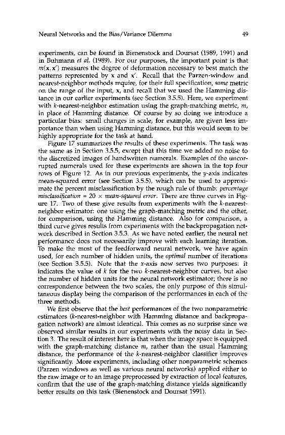
Neural Networks and the Bias/Variance Dilemma 49
experiments, can be found in Bienenstock and Doursat (1989, 1991) and in Buhmann et al. (1989). For our purposes, the important point is that m ( x , x’) measures the degree of deformation necessary to best match the patterns represented by x and x’. Recall that the Parzen-window and nearest-neighbor methods require, for their full specification, some metric on the range of the input, x, and recall that we used the Hamming dis- tance in our earlier experiments (see Section 3.5.5). Here, we experiment with k-nearest-neighbor estimation using the graph-matching metric, m, in place of Hamming distance. Of course by so doing we introduce a particular bias: small changes in scale, for example, are given less im- portance than when using Hamming distance, but this would seem to be highly appropriate for the task at hand.
Figure 17 summarizes the results of these experiments. The task was the same as in Section 3.5.5, except that this time we added no noise to the discretized images of handwritten numerals. Examples of the uncor- rupted numerals used for these experiments are shown in the top four rows of Figure 12. As in our previous experiments, the y-axis indicates mean-squared error (see Section 3.5.5), which can be used to approxi- mate the percent misclassification by the rough rule of thumb: percentage misclassification = 20 x mean-squared error. There are three curves in Fig- ure 17. Two of these give results from experiments with the k-nearest- neighbor estimator: one using the graph-matching metric and the other, for comparison, using the Hamming distance. Also for comparison, a third curve gives results from experiments with the backpropagation net- work described in Section 3.5.3. As we have noted earlier, the neural net performance does not necessarily improve with each learning iteration. To make the most of the feedforward neural network, we have again used, for each number of hidden units, the optimal number of iterations (see Section 3.5.5). Note that the x-axis now serves two purposes: it indicates the value of k for the two k-nearest-neighbor curves, but also the number of hidden units for the neural network estimator; there is no correspondence between the two scales, the only purpose of this simul- taneous display being the comparison of the performances in each of the three methods.
We first observe that the best performances of the two nonparametric estimators (k-nearest-neighbor with Hamming distance and backpropa- gation network) are almost identical. This comes as no surprise since we observed similar results in our experiments with the noisy data in Sec- tion 3. The result of interest here is that when the image space is equipped with the graph-matching distance m, rather than the usual Hamming distance, the performance of the k-nearest-neighbor classifier improves significantly. More experiments, including other nonparametric schemes (Parzen windows as well as various neural networks) applied either to the raw image or to an image preprocessed by extraction of local features, confirm that the use of the graph-matching distance yields significantly better results on this task (Bienenstock and Doursat 1991).

50 S. Geman, E. Bienenstock, and R. Doursat
backpropgation --%
H : : ’ 5 I0 IS 20
k, H.U.
Figure 1 7 Classification of handwritten numerals: performance as a function of the number k of neighbors in a k-nearest-neighbor estimator (curves marked “Hamming” and “elastic matching”) and the number of hidden units in a feed- forward neural network trained by error backpropagation (curve marked “back- propagation”). The two curves representing k-nearest-neighbor estimation are the results of experiments with two different measures of distance, and hence two notions of “neighbor.” The first is ordinary Hamming distance (the pat- terns are binary); the second is a measure of the deformation necessary to bring one pattern into another (the “elastic matching” metric).
Evidently then, the metric arising from graph matching is more suit- able for the problem at hand than the straightforward Hamming distance, arising from the pixel-array representation. By adopting a different repre- sentation, we have introduced a very significant bias, thereby achieving a better control of the variance. We believe, more generally, that adopting
Neural Networks and the Bias/Variance Dilemma 51
an appropriate data representation is an efficient means for designing the bias required for solving many hard problems in machine percep- tion. This view is of course shared by many authors. As Anderson and Rosenfeld (1988) put it: “A good representation does most of the work.”
7 Summary
To mimic substantial human behavior such as generic object recognition in real scenes - with confounding variations in orientation, lighting, texturing, figure-to-ground separation, and so on - will require complex machinery. Inferring this complexity from examples, that is, learning it, although theoretically achievable, is, for all practical matters, not feasible: too many examples would be needed. Important properties must be built-in or “hard-wired,” perhaps to be tuned later by experience, but not learned in any statistically meaningful way.
These conclusions and criticisms are probably shared by many au- thors. They can perhaps be argued most convincingly from the point of view of modern statistical theory, especially the theory of nonparametric inference. We have therefore presented a tutorial on the connection be- tween nonparametric inference and neural modeling as it stands today, and we have used the statistical framework, together with some simple numerical experiments, to argue for the limitations of learning in neural modeling.
Of course most neural modelers do not take tabula rasa architectures as serious models of the nervous system; these are viewed as providing a mere starting point for the study of adaptation and self-organization. Such an approach is probably meant as a convenience, a way of concen- trating on the essential issue of finding neurally plausible and effective learning algorithms. It strikes us, however, that identifying the right “preconditions” is the substantial problem in neural modeling. More specifically, it is our opinion that categorization must be largely built in, for example, by the use of generic mechanisms for representation, and that identifying these mechanisms is at the same time more difficult and more fundamental than understanding learning per se.
Acknowledgments
We are indebted to Isabelle Guyon and the AT&T Bell Laboratories for providing the data set of handwritten numerals used in our experiments, and to Nathan Intrator for a careful reading of the manuscript and many useful comments. S. G. was supported by Army Research Office Contract DAAL03-86-K-0171 to the Center for Intelligent Control Systems, Na- tional Science Foundation Grant DMS-8813699, Office of Naval Research
52 S. Geman, E. Bienenstock, and R. Doursat
Contract N00014-88-K-0289, and the General Motors Research Labora- tories. E. B. was supported by grants from the Commission of Euro- pean Communities (B.R.A.I.N. ST2J-0416) and the French MinistGre de la Recherche (87C0187).
References
Ackley, D. H., Hinton, G. E., and Sejnowski, T. J. 1985. A learning algorithm for Boltzmann machines. Cog. Sci. 9, 147-169.
Akaike, H. 1973. Information theory and an extension of the maximum likeli- hood principle. In Proceedings of the 2nd International Symposium on Informa- tion Theory, B. N. Petrov and F. Csaki, eds., pp. 267-281. Akademia Kiado, Budapest.
Amari, S. I. 1967. A theory of adaptive pattern classifiers. I E E E Transact. Elect. Computers EC-16, 299-307.
Amari, S. I. 1990. Dualistic geometry of the manifold of higher-order neurons. Tech. Rep. METR 90-17, Department of Mathematical Engineering and In- strumentation Physics, University of Tokyo, Bunkyo-Ku, Tokyo.
Amari, S. I., Kurata, K., and Nagaoka, H. 1990. Differential geometry of Boltz- mann machines. Tech. Rep., Department of Mathematical Engineering and Instrumentation Physics, University of Tokyo, Bunkyo-Ku, Tokyo.
Amit, Y., Grenander, U., and Piccioni, M. 1991. Structural image restoration through deformable templates. I. A m . Statist. Assoc. 86, 376-387.
Anderson, J. A., and Rosenfeld, E. 1988. Neurocomputing, Foundations of Research, p. 587. MIT Press, Cambridge MA.
Anderson, J. A., Silverstein, J. W., Ritz, S. A., and Jones, R. S. 1977. Distinctive features, categorical perception, and probability learning: Some applications of a neural model. Psychol. Rev. 84, 413451.
Anderson, J. A., Rossen, M. L., Viscuso, S. R., and Sereno, M. E. 1990. Ex- periments with representation in neural networks: Object motion, speech, and arithmetic. In Synergetics of Cognition, H. Haken and M. Stadler, eds. Springer-Verlag, Berlin.
Azencott, R. 1990. Synchronous Boltzmann machines and Gibbs fields: Learn- ing algorithms. In Neurocomputing, Algorithms, Architectures and Applica- tions, F. Fogelman-Soulie and J. Herault, eds., pp. 51-63. NATO AS1 Series, Vol. F68. Springer-Verlag, Berlin.
Bajcsy, R., and Kovacic, S. 1989. Multiresolution elastic matching. Comput. Vision, Graphics, Image Process. 46, 1-21.
Baldi, P., and Hornik, K. 1989. Neural networks and principal component anal- ysis: Learning from examples without local minima. Neural Networks 2,
Barron, A. R. 1989. Statistical properties of artificial neural networks. Proc. of 53-58.
the 28th Conf. Decision Control, Tampa, Florida, 280-285.
Neural Networks and the Bias/Variance Dilemma 53
Barron, A. R. 1991. Complexity regularization with application to artificial neural networks. In Nonparametric Functional Estimation and Related Topics, G. Roussas, ed., pp. 561-576. Kluwer, Dordrecht.
Barron, A. R., and Barron, R. L. 1988. Statistical learning networks: A unifying view. In Computing Science and Statistics, Proceedings of the 20th Symposium Interface, E. Wegman, ed., pp. 192-203. American Statistical Association, Washington, DC.
Baum, E. B. 1990a. The perceptron algorithm is fast for nonmalicious distribu- tions. Neural Comp. 2, 248-260.
Baum, E. B. 1990b. When are k-nearest-neighbor and backpropagation accurate for feasible-sized sets of examples? In Proceedings Eurasip Workshop on Neural Networks, L. B. Almeida and C. J. Wellekens, eds., pp. 2-25. Springer-Verlag, Berlin.
Baum, E. B., and Haussler, D. 1989. What size net gives vaIid generalization? Neural Comp. 1, 151-160.
Baum, L. E. 1972. An inequality and associated maximization technique in statistical estimation for probabilistic functions of Markov processes. In- equalities 3, 1-8.
Bellman, R. E. 1961. Adaptive Control Processes. Princeton University Press, Princeton, NJ.
Bienenstock, E., and Doursat, R. 1989. Elastic matching and pattern recogni- tion in neural networks. In Neural Networks: From Models to Applications, L. Personnaz and G. Dreyfus, eds., pp. 472-482. IDSET, Paris.
Bienenstock, E., and Doursat, R. 1991. Issues of representation in neural net- works, In Representations of Vision: Trends and Tacit Assumptions in Vision Reseauch, A. Gorea, ed., pp. 47-67. Cambridge University Press, Cambridge.
Bourlard, H., and Kamp, Y. 1988. Auto-association by multi-layer perceptrons and singular value decomposition. Biol. Cybernet. 59, 291-294.
Bourlard, H., and Wellekens, C. J. 1990. Links between Markov models and multilayer perceptrons. I E E E Transact. Pattern Anal. Machine Intell. 12, 1167- 1178.
Breiman, L., and Friedman, J. H. 1985. Estimating optimal transformations for multiple regression and correlation. 1. Am. Stat. Assoc. 80, 580-619.
Breiman, L., Friedman, J. H., Olshen, R. A., and Stone, C. J. 1984. Classification and Regression Trees. Wadsworth, Belmont, CA.
Buhmann, J., Lange, J., von der Malsburg, Ch., Vorbruggen, J. C., and Wiirtz, R. P. 1989. Object recognition in the dynamic link architecture: Parallel implementation on a transputer network. In Neural Networks: A Dynamic Systems Approach f o Machine Intelligence, B. Kosko, ed. Prentice Hall, New York.
Burr, D. J. 1980. Elastic matching of line drawings. IEEE Transact. Pattern Anal. Machine Intell. PAMI-3 6, 708-713.
Carnevali, P., and Patarnello, S. 1987. Exhaustive thermodynamic analysis of Boolean learning networks. Europhys. Lett. 4, 1199-1204.
Chauvin, Y. 1990. Dynamic behavior of constrained back-propagation networks. In Neural Information Processing Systems 11, D. S. Touretzky, ed., pp. 642-649.
54 S. Geman, E. Bienenstock, and R. Doursat
Morgan Kaufmann, San Mateo, CA. Collins, E., Ghosh, S., and Scofield, C. 1989. An application of a multiple neu-
ral network learning system to emulation of mortgage underwriting judge- ments. Nestor Inc., Providence, RI.
Cox, D. R. 1970. The Analysis of Binary Data. Methuen, London. Crick, F. 1989. The recent excitement about neural networks. Nature (London)
Cybenko, G. 1989. Approximations by superpositions of a sigmoidal function. Math. Control, Signals Syst. 2, 303-314.
Dempster, A. I?, Laird, N. M., and Rubin, D. 8. 1976. Maximum likelihood from incomplete data via the EM algorithm. J. R. Statist. SOC. B 39, 1-38.
Denker, J., Schwartz, D., Wittner, B., Solla, S., Howard, R., Jackel, L., and Hop- field, J. 1987. Automatic learning, rule extraction and generalization. Com-
Diaconis, P., and Freedman, D. 1986. On the consistency of Bayes estimates.
Duda, I<. O., and Hart, P. E. 1973. Pattern Classification and Scene Analysis. Wiley,
Dudley, R. M. 1987. Universal Donsker classes and metric entropy. A n n . Prob.
Faraway, J. J., and Jhun, M. 1990. Bootstrap choice o f bandwidth for density
Fischler, M., and Elschlager, R. 1973. The representation and matching of pic-
Fodor, J. A., and Pylyshyn, Z. 1988. Connectionism and cognitive architecture:
Friedman, J. H. 1991. Multivariate adaptive regression splines. Ann. Statist. 19,
Friedman, J. H., and Stuetzle, W. 1981. Projection pursuit regression. J. A m . Statist. Assoc. 76, 817-823.
Funahashi, K. 1989. On the approximate realization of continuous mappings by neural networks. Neural Networks 2, 183-192.
Gallinari, P., Thiria, S., and Fogelman, F. 1988. Multilayer perceptrons and data analysis. Proc. I E E E l C N N 88(1), 391-399.
Geman, S., and Hwang, C. 1982. Nonparametric maximum likelihood estima- tion by the method of sieves. Ann . Statist. 10, 401414.
Goldman, L., Weinberg, M., Weisberg, M., Olshen, R., Cook, E. F., Sargent, R. K., Lamas, G. A., Dennis, C., Wilson, C., Deckelbaum, L., Fineberg, H., and Stiratelli, R. 1982. A computer-derived protocol to aid in the diagnosis of emergency room patients with acute chest pain. New Engl. J. Med. 307,
Grenander, U. 1951. On empirical spectral analysis of stochastic processes. Ark.
Grenander, U. 1981. Abstract Inference. Wiley, New York. Grenander, U., Chow, Y. S., and Keenan, D. 1990. H A N D S , A Pattern Theoretic
337, 129-132.
plex Syst. 1, 877-922.
Ann. Statist. 14, 1-26.
New York.
15, 1306-1326.
estimation. J. A m . Statist. Assoc. 85, 1119-1122.
torial structures. I € € € Transact. Comput. 22, 67-92.
A critical analysis. Cognition 28, 3-71.
1-141.
588-596.
Matemat. 1, 503-531.

Neural Networks and the Bias/Variance Dilemma 55
Study of Biological Shapes. Springer-Verlag, New York. Guyon, I. 1988. Reseaux de neurones pour la reconnaissance des formes: archi-
tectures et apprentissage. Unpublished doctoral dissertation, University of Paris VI, December.
Hansen, L. K., and Salamon, P. 1990. Neural network ensembles. IEEE Transact. Pattern Anal. Machine Intell. PAMI-12(10), 993-1001.
Hardle, W. 1990. Smoothing Techniques with Implementation in S . Springer Series in Statistics. Springer-Verlag, New York.
Hardle, W., Hall, P., and Marron, J. S., 1988. How far are automatically chosen regression smoothing parameters from their optimum? J. Am. Statist. Assoc. 83, 86-95.
Hartman, E. J., Keeler, J. D., and Kowalski, J. M. 1990. Layered neural networks with gaussian hidden units as universal approximations. Neural Cornp. 2, 210-215.
Haussler, D. 1989a. Generalizing the PAC model: Sample size bounds from metric dimension-based uniform convergence results. Proc. 30th Ann. Symp. Foundations Cornput. Sci., IEEE.
Haussler, D. 1989b. Decision theoretic generalizations of the PAC model for neural net and other learning applications. Preprint.
Hinton, G. E., and Nowlan, S. J. 1990. The boostrap Widrow-Hoff rule as a cluster-formation algorithm. Neural Comp. 2, 355-362.
Hinton, G. E., and Sejnowski, T. J. 1986. Learning and relearning in Boltzmann machines. In Parallel Distributed Processing: Explorations in the Microstructure of Cognition. Vol. 1: Foundations, D. E. Rumelhart, J. L. McClelland, and the PDP group, eds., pp. 282-317. MIT Press, Cambridge, MA.
Hornik, M., Stinchcombe, M., and White, H. 1989. Multilayer feedforward networks are universal approximators. Neural Networks 2, 359-366.
Huber, P. J. 1985. Projection pursuit. Ann. Statist. 13, 435-475. Intrator, N. 1990. Feature extraction using an exploratory projection pursuit
neural network. Ph.D. Thesis, Division of Applied Mathematics, Brown University, Providence, RI.
Karnin, E. D., 1990. A simple procedure for pruning back-propagation trained neural networks. IEEE Transact. Neural Networks 1(2), 239-242.
Knoerr, A. 1988. Global models of natural boundaries: Theory and applica- tions. Ph.D. Thesis, Division of Applied Mathematics, Brown University, Providence, RI.
Le Cun, Y., Boser, B., Denker, J. S., Henderson, D., Howard, R. E., Hubbard, W., and Jackel, L. D. 1989. Backpropagation applied to handwritten zip code recognition. Neural Cornp. 1, 541-551.
Lippmann, R. P. 1987. An introduction to computing with neural nets. IEEE ASSP Mag. April, 4-22.
Lippmann, R. I? 1989. Review of neural networks for speech recognition. Neural Comp. 1, 1-39.
Lorenzen, T. J. 1988. Setting realistic process specification limits - A case study. General Motors Research Labs. Publication GMR-6389, Warren, MI.

56 S. Geman, E. Bienenstock, and R. Doursat
Maechler, M., Martin, D., Schimert, J., Csoppenszky, M., and Hwang, J. N. 1990. Projection pursuit learning networks for regression. Preprint.
Marron, J. S. 1988. Automatic smoothing parameter selection: A survey. Em- pirical Econ. 13, 187-208.
Martin, G. L., and Pittman, J. A. 1991. Recognizing hand-printed letters and digits using backpropagation learning. Neural Comp. 3, 258-267.
Morgan, N., and Bourlard, H. 1990. Generalization and parameter estimation in feedforward nets: Some experiments. In Neural Informafion Processing Systems II, D. S. Touretzky, ed., pp. 630-637. Morgan Kaufmann, San Mateo, CA .
Mozer, M. C., and Smolensky, I? 1989. Skeletonization: A technique for trim- ming the fat from a network via relevance assessment. In Advances in Neural Information Processing Systems I , D. S. Touretzky, ed., pp. 107-115. Morgan Kaufmann, San Mateo, CA.
OSullivan, F., and Wahba, G. 1985. A cross validated Bayesian retrieval al- gorithm for non-linear remote sensing experiments. J. Comput. Phys. 59, 441-455.
Poggio, T., and Girosi, F. 1990. Regularization algorithms for learning that are equivalent to multilayer networks. Science 247,978-982.
Pollard, D. 1984. Convergence of Stochastic Processes. Springer-Verlag, Berlin. Rissanen, J. 1986. Stochastic complexity and modeling. Ann. Statist. 14(3),
108&1100. Rosenblatt, F. 1962. Principles of Neurodynamics: Perceptrons and the Theory of
Brain Mechanisms. Spartan Books, Washington. Rumelhart, D. E., Hinton, G. E., and Williams, R. J. 1986a. Learning internal
representations by error propagation. In Parallel Distributed Processing: Ex- plorations in the Microstructure of Cognition. Vol. 2 : Foundations, D. E. Rumel- hart, J. L. McClelland, and the PDP group, eds., pp. 318-362. MIT Press, Cambridge, MA.
Rumelhart, D. E., Hinton, G. E., and Williams, R. J. 1986b. Learning represen- tations by backpropagating errors. Nature (London) 323, 533-536.
Schuster, E. F., and Gregory, G. G. 1981. On the nonconsistency of maxi- mum likelihood nonparametric density estimators. In Compiiter Science and Statistics: Proceedings of the 23th Symposium on the Interface, W. F. Eddy, ed., pp. 295-298. Springer-Verlag, New York.
Schwartz, D. B., Samalam, V. K., Solla, S. A., and Denker, J. S. 1990. Exhaustive learning. Neural Comp. 2, 374-385.
Scott, D., and Terrell, G . 1987. Biased and unbiased cross-validation in density estimation. J. Am. Statist. Assoc. 82, 1131-1146.
Shepard, R. N. 1989. Internal representation of universal regularities: A chal- lenge for connectionism. In Neural Connections, Mental Computation, L. Nadel, L. A. Cooper, P. Culicover, and R. M. Harnish, eds., pp. 104-134. Brad- ford /MIT Press, Cambridge, MA, London, England.
Smolensky, P. 1988. On the proper treatment of connectionism. Behav. Brain Sci.
Solla, S. A. 1989. Learning and generalization in layered neural networks: The 11, 1-74.

Neural Networks and the BiasNariance Dilemma 57
contiguity problem. In Neural Networks: From Models to Applications, L. Per- sonnaz and G. Dreyfus, eds., pp. 168-177. IDSET, Paris.
Stone, M. 1974. Cross-validatory choice and assessment of statistical predictors (with discussion). J. R. Statist. SOC. B36, 111-147.
Tishby, N., Levin, E., and Solla, S. A. 1989. Consistent inferences of probabilities in layered networks: Predictions and generalization. In I JCNN International Joint Conference on Neural Networks, Vol. I I , pp. 403409, IEEE, New York.
Vapnik, V. N. 1982. Estimation of Dependences Based on Empirical Data. Springer- Verlag, New York.
Vardi, Y., Shepp, L. A., and Kaufman, L. 1985. A statistical model for positron emission tomography (with comments). J. Am. Statist. Assoc. 80, 8-37.
Veklerov, E., and Llacer, J. 1987. Stopping rule for the MLE algorithm based on statistical hypothesis testing. IEEE Transact. Med. Imaging 6, 313-319.
von der Malsburg, Ch. 1981. The correlation theory of brain function. Inter- nal Report 83-2, Max Planck Institute for Biophysical Chemistry, Dept. of Neurobiology, Gottingen, W.-Germany.
von der Malsbhrg, Ch. 1986. Am I thinking assemblies? In Brain Theory, G. Palm and A. Aertsen, eds., pp. 161-176. Springer-Verlag, Heidelberg.
von der Malsburg, Ch., and Bienenstock, E. 1986. Statistical coding and short- term synaptic plasticity: A scheme for knowledge representation in the brain. In Disordered Systems and Biological Organization, E. Bienenstock, F. Fo- gelman, and G. Weisbuch eds., pp. 247-272. Springer-Verlag, Berlin.
Wahba, G. 1979. Convergence rates of ”thin plate” smoothing splines when the data are noisy. In Smoothing Techniques for Curve Estimation, T. Gasser and M. Rosenblatt, eds., pp. 233-245. Springer-Verlag, Heidelberg.
Wahba, G. 1982. Constrained regularization for ill posed linear operator equa- tions, with applications in meteorology and medicine. In Statistical Decision Theory and Related Topics III , Vol. 2, S. S. Gupta and J. 0. Berger, eds., pp. 383- 418. Academic Press, New York.
Wahba, G. 1984. Cross validated spline methods for the estimation of multivari- ate functions from data on functionals. In Statistics: An Appraisal, Proceedings 50th Anniversary Conference Iowa State Statistical Laboratory, H. A. David and H. T. David, eds., pp. 205-235. Iowa State Univ. Press, Ames.
Wahba, G. 1985. A comparison of GCV and GML for choosing the smoothing parameter in the generalized spline smoothing problem. Ann. Statist. 13, 1378-1 402.
Wahba, G. and Wold, S. 1975. A completely automatic French curve: fitting spline functions by cross validation. Commun. Statist. 4, 1-17.
Waibel, A,, Hanazawa, T., Hinton, G., Shikano, K., and Lang, K. 1988. Phoneme recognition using time-delay networks. Proc. ICASSP-88, New York.
White, H. 1988. Multilayer feedforward networks can learn arbitrary mappings: Connectionist nonparametric regression with automatic and semi-automatic determination of network complexity. UCSD Department of Economics Dis- cussion Paper.
White, H. 1989. Learning in artificial neural networks: A statistical perspective. Neural Comp. 1, 425464.

58 S. Geman, E. Bienenstock, and R. Doursat
White, H. 1990. Connectionists nonparametric regression: multilayer feedfor-
Widrow, B. 1973. The rubber mask technique, Part I. Pattern Recognition 5, 175-
Yuille, A. 1990. Generalized deformable models, statistical physics, and match-
ward networks can learn arbitrary mappings. Neural Networks 3, 535-549.
211.
ing problems. Neural Comp. 2, 1-24.
Received 4 May 1991; accepted 3 June 1991.