CS536: Machine Learning Artificial Neural Networks Neural Networks
32
CS536: Machine Learning Artificial Neural Networks Fall 2005 Ahmed Elgammal Dept of Computer Science Rutgers University CS 536 – Artificial Neural Networks - -2 Neural Networks Biological Motivation: Brain • Networks of processing units (neurons) with connections (synapses) between them • Large number of neurons: 10 11 • Large connectitivity: each connected to, on average, 10 4 others • Switching time 10 -3 second • Parallel processing • Distributed computation/memory • Processing is done by neurons and the memory is in the synapses • Robust to noise, failures
Transcript of CS536: Machine Learning Artificial Neural Networks Neural Networks

1
CS536: Machine Learning
Artificial Neural Networks
Fall 2005Ahmed Elgammal
Dept of Computer ScienceRutgers University
CS 536 – Artificial Neural Networks - - 2
Neural Networks
Biological Motivation: Brain• Networks of processing units (neurons) with connections (synapses)
between them• Large number of neurons: 1011
• Large connectitivity: each connected to, on average, 104 others• Switching time 10-3 second• Parallel processing• Distributed computation/memory• Processing is done by neurons
and the memory is in the synapses• Robust to noise, failures
2
CS 536 – Artificial Neural Networks - - 3
Neural Networks
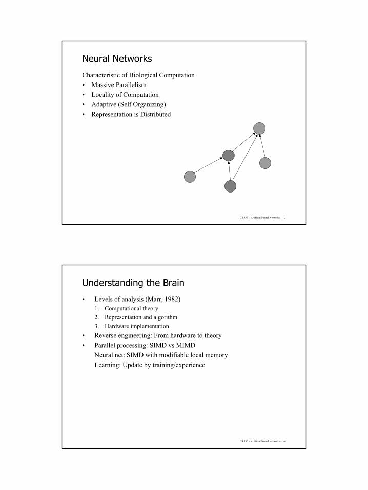
Characteristic of Biological Computation• Massive Parallelism• Locality of Computation• Adaptive (Self Organizing)• Representation is Distributed
CS 536 – Artificial Neural Networks - - 4
Understanding the Brain
• Levels of analysis (Marr, 1982)1. Computational theory2. Representation and algorithm3. Hardware implementation
• Reverse engineering: From hardware to theory• Parallel processing: SIMD vs MIMD
Neural net: SIMD with modifiable local memoryLearning: Update by training/experience
3
CS 536 – Artificial Neural Networks - - 5
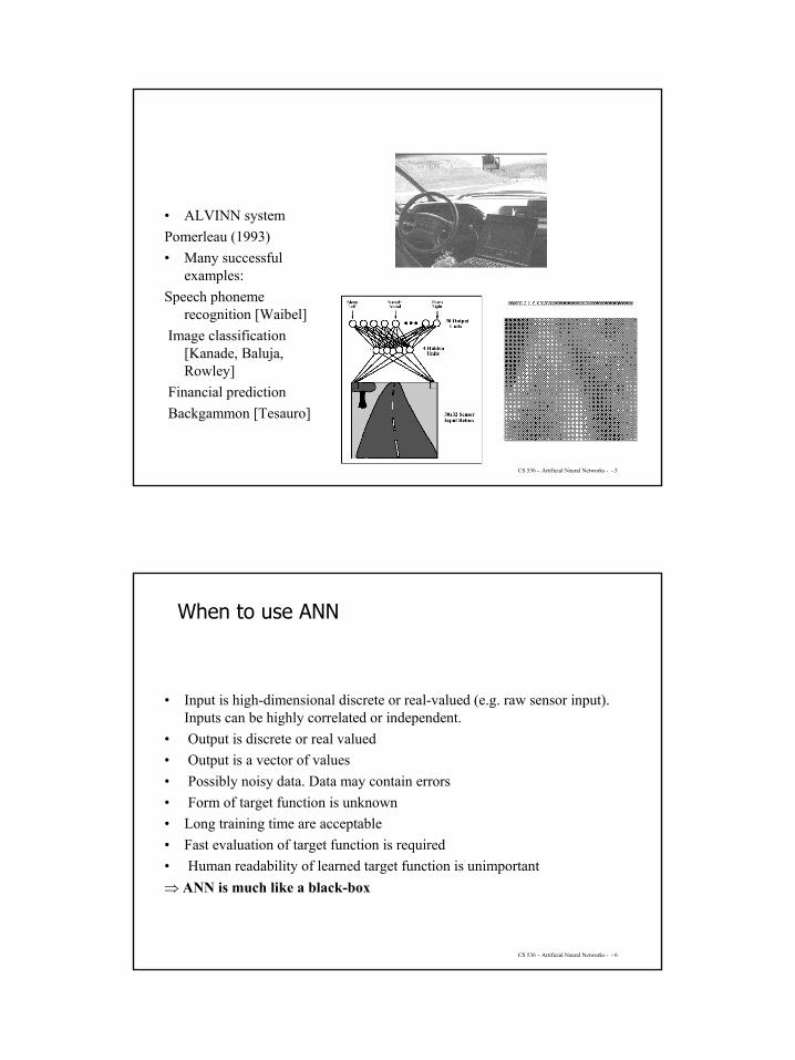
• ALVINN system Pomerleau (1993)• Many successful
examples:Speech phoneme
recognition [Waibel]Image classification
[Kanade, Baluja, Rowley]
Financial predictionBackgammon [Tesauro]
CS 536 – Artificial Neural Networks - - 6
When to use ANN
• Input is high-dimensional discrete or real-valued (e.g. raw sensor input). Inputs can be highly correlated or independent.
• Output is discrete or real valued• Output is a vector of values• Possibly noisy data. Data may contain errors• Form of target function is unknown• Long training time are acceptable• Fast evaluation of target function is required• Human readability of learned target function is unimportant⇒ ANN is much like a black-box
4
CS 536 – Artificial Neural Networks - - 7
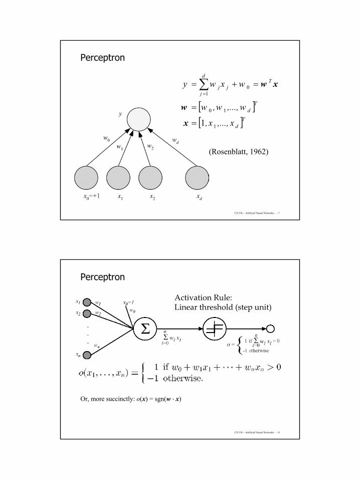
Perceptron
(Rosenblatt, 1962)
[ ][ ]Td
Td
Td
jjj
x,...,x,
w,...,w,w
wxwy
1
10
01
1=
=
=+= ∑=
x
w
xw
CS 536 – Artificial Neural Networks - - 8
Perceptron
Or, more succinctly: o(x) = sgn(w ⋅ x)
Activation Rule:Linear threshold (step unit)
5
CS 536 – Artificial Neural Networks - - 9
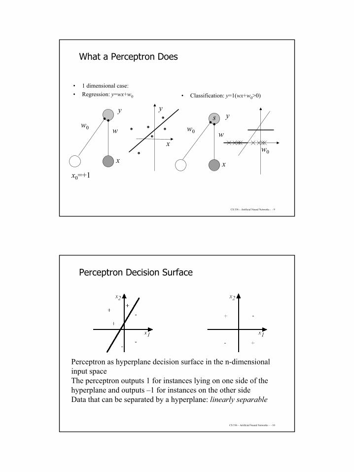
What a Perceptron Does
• 1 dimensional case:• Regression: y=wx+w0 • Classification: y=1(wx+w0>0)
ww0
y
x
x0=+1
ww0
y
x
s
w0
y
x
CS 536 – Artificial Neural Networks - - 10
Perceptron Decision Surface
Perceptron as hyperplane decision surface in the n-dimensional input spaceThe perceptron outputs 1 for instances lying on one side of the hyperplane and outputs –1 for instances on the other sideData that can be separated by a hyperplane: linearly separable
6
CS 536 – Artificial Neural Networks - - 11
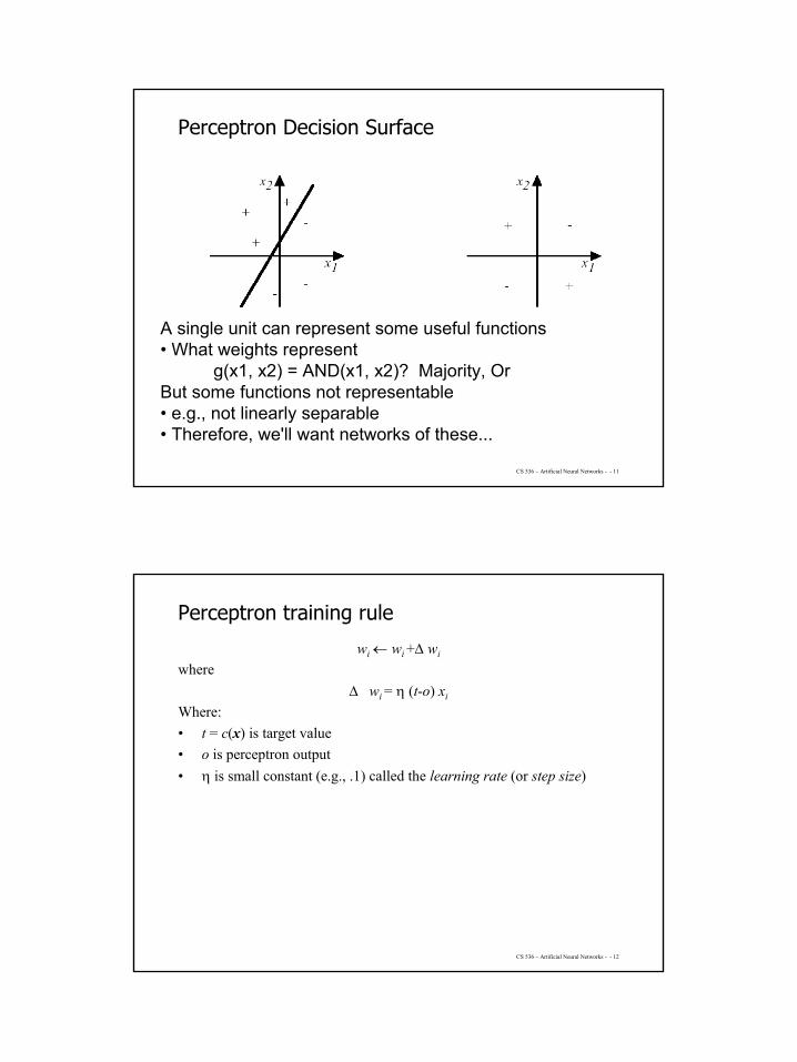
Perceptron Decision Surface
A single unit can represent some useful functions• What weights represent
g(x1, x2) = AND(x1, x2)? Majority, OrBut some functions not representable• e.g., not linearly separable• Therefore, we'll want networks of these...
CS 536 – Artificial Neural Networks - - 12
Perceptron training rule
wi ← wi +∆ wi
where∆ wi = η (t-o) xi
Where:• t = c(x) is target value• o is perceptron output• η is small constant (e.g., .1) called the learning rate (or step size)
7
CS 536 – Artificial Neural Networks - - 13
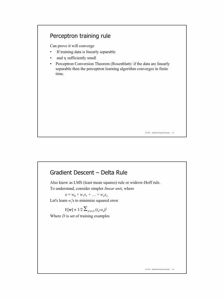
Perceptron training rule
Can prove it will converge• If training data is linearly separable• and η sufficiently small• Perceptron Conversion Theorem (Rosenblatt): if the data are linearly
separable then the perceptron learning algorithm converges in finite time.
CS 536 – Artificial Neural Networks - - 14
Gradient Descent – Delta Rule
Also know as LMS (least mean squares) rule or widrow-Hoff rule.To understand, consider simpler linear unit, where
o = w0 + w1x1 + … + wnxn
Let's learn wi's to minimize squared error
E[w] ≡ 1/2 Σd in D (td-od)2
Where D is set of training examples

8
CS 536 – Artificial Neural Networks - - 15
Error Surface
CS 536 – Artificial Neural Networks - - 16
Gradient Descent
Gradient∇E [w] = [∂E/∂w0,∂E/∂w1,…,∂E/∂wn]When interpreted as a vector in weight space, the gradient specifies the
direction that produces the steepest increase in ETraining rule:
∆w = -η ∇E [w]in other words:
∆wi = -η ∂E/∂wi
This results in the following update rule:
∆wi = η Σd (td-od) (xi,d)

9
CS 536 – Artificial Neural Networks - - 17
Gradient of Error
∂E/∂wi
= ∂/∂wi 1/2 Σd (td-od)2
= 1/2 Σd ∂/∂wi (td-od)2
= 1/2 Σd 2 (td-od) ∂/∂wi (td-od)
= Σd (td-od) ∂/∂wi (td-w xd)
= Σd (td-od) (-xi,d)
Learning Rule:∆wi = -η ∂E/∂wi
⇒ ∆wi = η Σd (td-od) (xi,d)
CS 536 – Artificial Neural Networks - - 18
Stochastic Gradient Descent
Batch mode Gradient Descent:Do until satisfied1. Compute the gradient ∇ED [w] 2. w ← w - ∇ED [w] Incremental mode Gradient Descent:Do until satisfied• For each training example d in D
1. Compute the gradient ∇Ed [w] 2. w ← w - ∇Ed [w]
10
CS 536 – Artificial Neural Networks - - 19
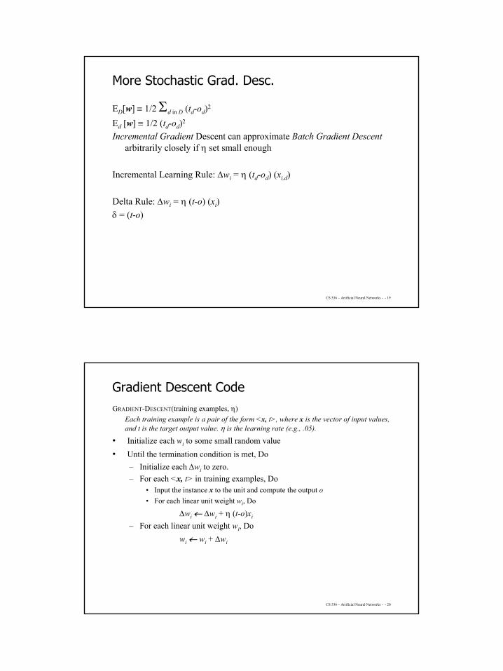
More Stochastic Grad. Desc.
ED[w] ≡ 1/2 Σd in D (td-od)2
Ed [w] ≡ 1/2 (td-od)2
Incremental Gradient Descent can approximate Batch Gradient Descent arbitrarily closely if η set small enough
Incremental Learning Rule: ∆wi = η (td-od) (xi,d)
Delta Rule: ∆wi = η (t-o) (xi)δ = (t-o)
CS 536 – Artificial Neural Networks - - 20
Gradient Descent CodeGRADIENT-DESCENT(training examples, η)
Each training example is a pair of the form <x, t>, where x is the vector of input values, and t is the target output value. η is the learning rate (e.g., .05).
• Initialize each wi to some small random value• Until the termination condition is met, Do
– Initialize each ∆wi to zero.– For each <x, t> in training examples, Do
• Input the instance x to the unit and compute the output o• For each linear unit weight wi, Do
∆wi ← ∆wi + η (t-o)xi
– For each linear unit weight wi, Dowi ← wi + ∆wi
11
CS 536 – Artificial Neural Networks - - 21
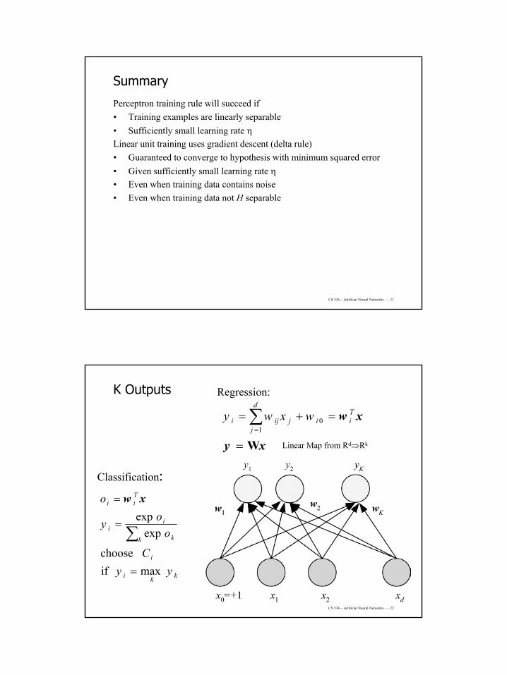
Summary
Perceptron training rule will succeed if• Training examples are linearly separable• Sufficiently small learning rate ηLinear unit training uses gradient descent (delta rule)• Guaranteed to converge to hypothesis with minimum squared error• Given sufficiently small learning rate η• Even when training data contains noise• Even when training data not H separable
CS 536 – Artificial Neural Networks - - 22
K Outputs
kki
i
k k
ii
Tii
yyC
ooy
o
maxif choose
expexp
=
=
=
∑
xw
Classification:
Regression:
xy
xw
W=
=+= ∑=
Tii
d
jjiji wxwy 0
1
Linear Map from Rd⇒Rk
12
CS 536 – Artificial Neural Networks - - 23
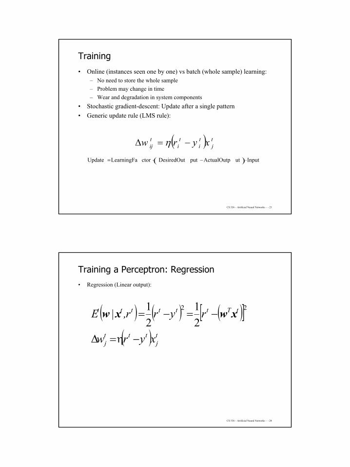
Training
• Online (instances seen one by one) vs batch (whole sample) learning:– No need to store the whole sample– Problem may change in time– Wear and degradation in system components
• Stochastic gradient-descent: Update after a single pattern• Generic update rule (LMS rule):
( )( ) InpututActualOutpputDesiredOutctorLearningFaUpdate ⋅−⋅=
−=∆ tj
ti
ti
tij xyrw η
CS 536 – Artificial Neural Networks - - 24
Training a Perceptron: Regression• Regression (Linear output):
( ) ( ) ( )[ ]( ) t
jttt
j
tTtttttt
xyrw
ryrr,E
−η=
−=−=
∆
22
21
21| xwxw
13
CS 536 – Artificial Neural Networks - - 25
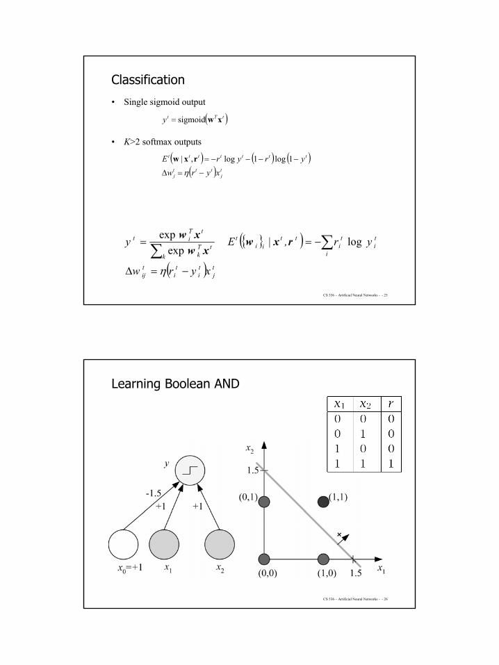
Classification
• Single sigmoid output
• K>2 softmax outputs
( )
( ) ( ) ( )( ) t
jttt
j
ttttttt
tTt
xyrwyryrE
y
−=∆
−−−−=
=
η
1 log 1 log ,|
sigmoid
rxw
xw
{ }( )
( ) tj
ti
ti
tij
i
ti
ti
ttii
t
ktT
k
tTit
xyrw
yr,Ey
−=∆
−== ∑∑η
log | exp
exp rxwxw
xw
CS 536 – Artificial Neural Networks - - 26
Learning Boolean AND

14
CS 536 – Artificial Neural Networks - - 27
XOR
• No w0, w1, w2 satisfy:
(Minsky and Papert, 1969)
0000
021
01
02
0
≤++>+>+≤
wwwwwwww
CS 536 – Artificial Neural Networks - - 28
Multilayer Perceptrons
(Rumelhart et al., 1986)
( )
( )[ ]∑
∑
=
=
+−+=
=
+==
d
j hjhj
Thh
H
hihih
Tii
wxw
z
vzvy
1 0
10
exp11
sigmoid xw
zv
15
CS 536 – Artificial Neural Networks - - 29
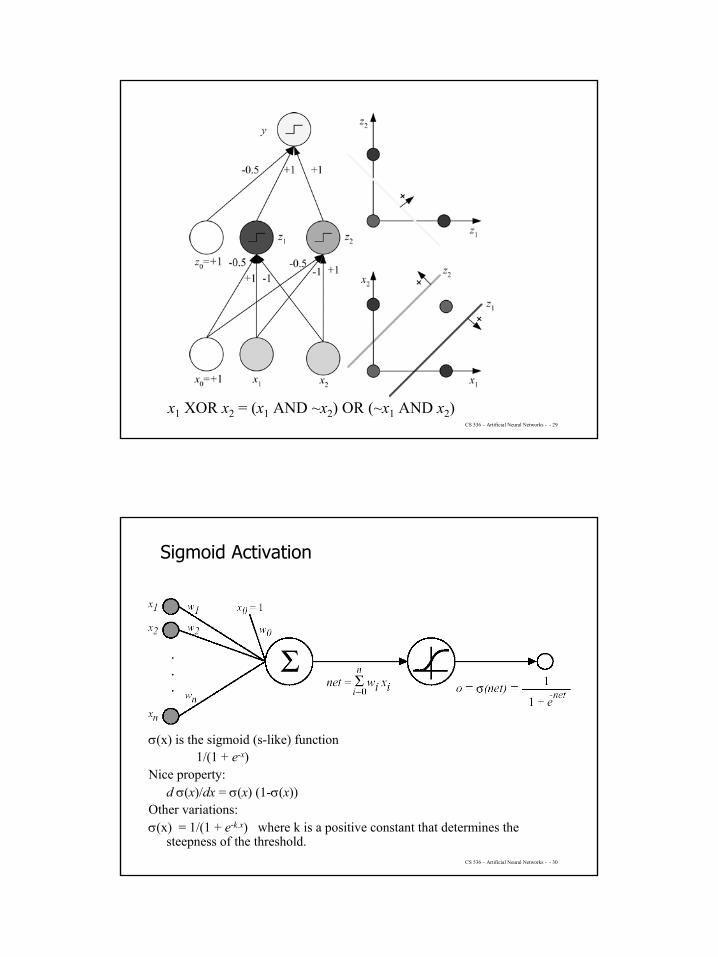
x1 XOR x2 = (x1 AND ~x2) OR (~x1 AND x2)
CS 536 – Artificial Neural Networks - - 30
Sigmoid Activation
σ(x) is the sigmoid (s-like) function1/(1 + e-x)
Nice property:d σ(x)/dx = σ(x) (1-σ(x))
Other variations: σ(x) = 1/(1 + e-k.x) where k is a positive constant that determines the
steepness of the threshold.
16
CS 536 – Artificial Neural Networks - - 31
CS 536 – Artificial Neural Networks - - 32
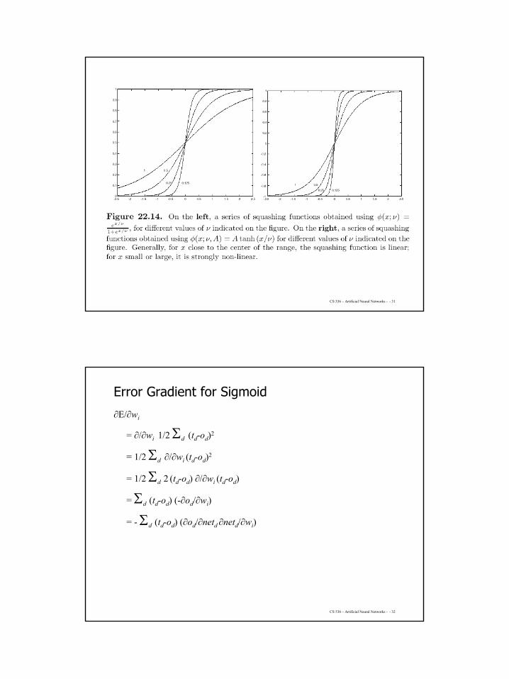
Error Gradient for Sigmoid
∂E/∂wi
= ∂/∂wi 1/2 Σd (td-od)2
= 1/2 Σd ∂/∂wi (td-od)2
= 1/2 Σd 2 (td-od) ∂/∂wi (td-od)
= Σd (td-od) (-∂od/∂wi)
= - Σd (td-od) (∂od/∂netd ∂netd/∂wi)
17
CS 536 – Artificial Neural Networks - - 33
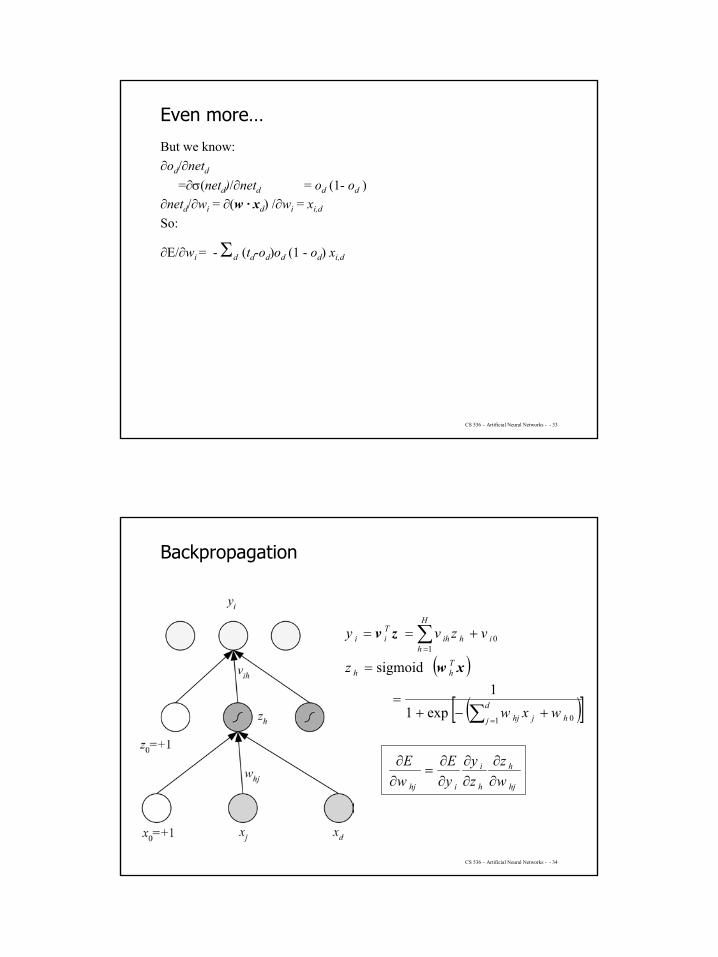
Even more…
But we know:∂od/∂netd
=∂σ(netd)/∂netd = od (1- od )∂netd/∂wi = ∂(w · xd) /∂wi = xi,d
So:
∂E/∂wi = - Σd (td-od)od (1 - od) xi,d
CS 536 – Artificial Neural Networks - - 34
Backpropagation
( )
( )[ ]
hj
h
h
i
ihj
d
j hjhj
Thh
H
hihih
Tii
wz
zy
yE
wE
wxw
z
vzvy
∂∂
∂∂
∂∂
=∂∂
+−+=
=
+==
∑
∑
=
=
exp11
sigmoid
1 0
10
xw
zv
18
CS 536 – Artificial Neural Networks - - 35
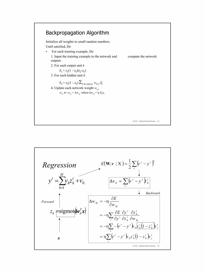
Backpropagation AlgorithmInitialize all weights to small random numbers.Until satisfied, Do• For each training example, Do
1. Input the training example to the network and compute the network outputs2. For each output unit k
δk = ok(1 - ok)(tk-ok)3. For each hidden unit h
δh = oh(1 - oh) Σk in outputs wh,k δk
4. Update each network weight wi,jwi,j ← wi,j + ∆wi,j where ∆wi,j = η δjai
CS 536 – Artificial Neural Networks - - 36
( ) ( )( ) ( ) t
jth
th
th
tt
tj
th
th
th
tt
hj
th
th
t
tt
hjhj
xzzvyr
xzzvyr
wz
zy
yE
wEw
−−η=
−−−η−=
∂∂
∂∂
∂∂
η−=
∂∂
η−=
∑
∑
∑
1
1
∆
Regression
Forward
Backward
x
( )xwThhz sigmoid=
∑=
+=H
h
thh
t vzvy1
0
( ) ( )221| ∑ −=
t
tt yr,E XvW
( ) th
t
tth zyrv ∑ −=∆
19
CS 536 – Artificial Neural Networks - - 37
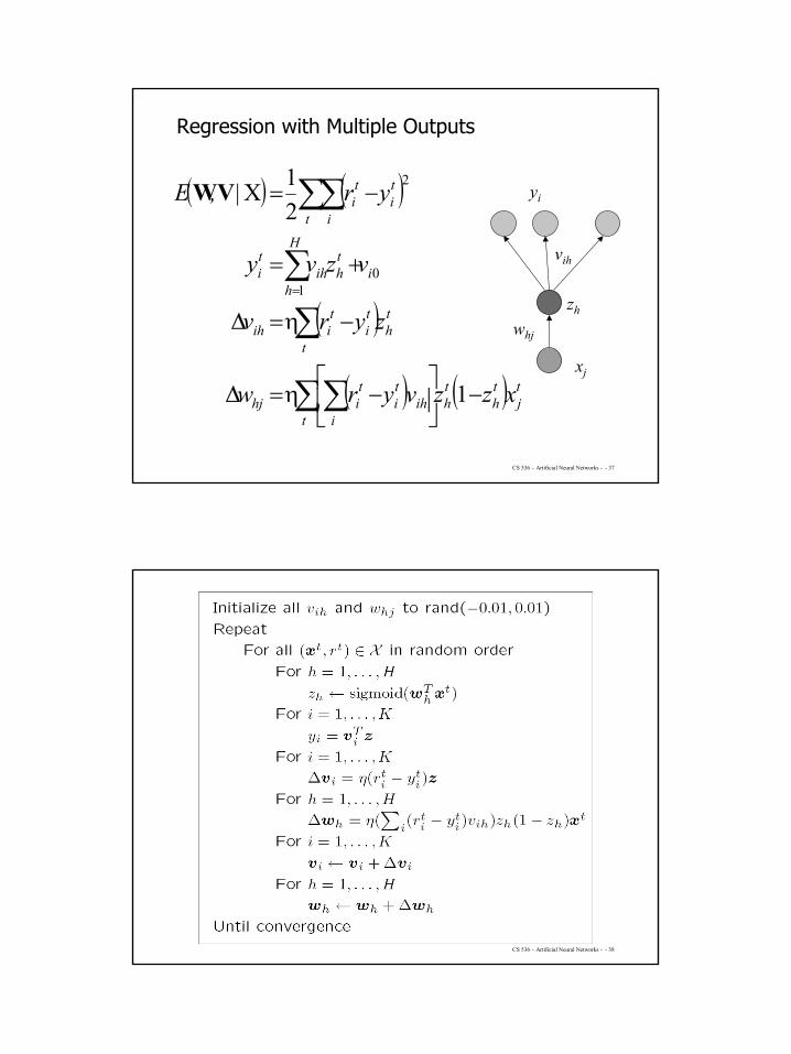
Regression with Multiple Outputs
zh
vih
yi
xj
whj
( ) ( )
( )
( ) ( ) tj
th
th
t iih
ti
tihj
th
t
ti
tiih
i
H
h
thih
ti
t i
ti
ti
xzzvyrw
zyrv
vzvy
yr,E
−
−η=
−η=
+=
−=
∑∑
∑
∑
∑∑
=
1
21|
01
2
∆
∆
XVW
CS 536 – Artificial Neural Networks - - 38
20
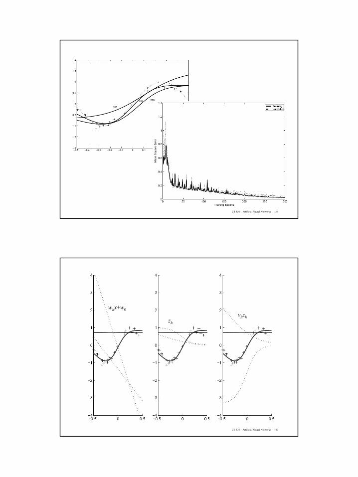
CS 536 – Artificial Neural Networks - - 39
CS 536 – Artificial Neural Networks - - 40
whx+w0
zh
vhzh
21
CS 536 – Artificial Neural Networks - - 41
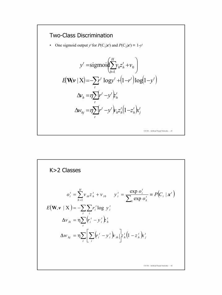
Two-Class Discrimination
• One sigmoid output yt for P(C1|xt) and P(C2|xt) ≡ 1-yt
( ) ( ) ( )( )( ) ( ) t
jth
thh
t
tthj
th
t
tth
t
tttt
H
h
thh
t
xzzvyrw
zyrv
yryr,E
vzvy
−−=∆
−=∆
−−+−=
+=
∑
∑
∑
∑=
1
1 log 1 log |
sigmoid1
0
η
η
XvW
CS 536 – Artificial Neural Networks - - 42
K>2 Classes
( )
( )
( )
( ) ( ) tj
th
th
t iih
ti
tihj
th
t
ti
tiih
t i
ti
ti
ti
ktk
tit
i
H
hi
thih
ti
xzzvyrw
zyrv
yr,E
CPo
oyvzvo
−
−η=
−η=
−=
≡=+=
∑ ∑
∑
∑∑∑∑
=
1
log|
|exp
exp 1
0
∆
∆
Xv
x
W
22
CS 536 – Artificial Neural Networks - - 43
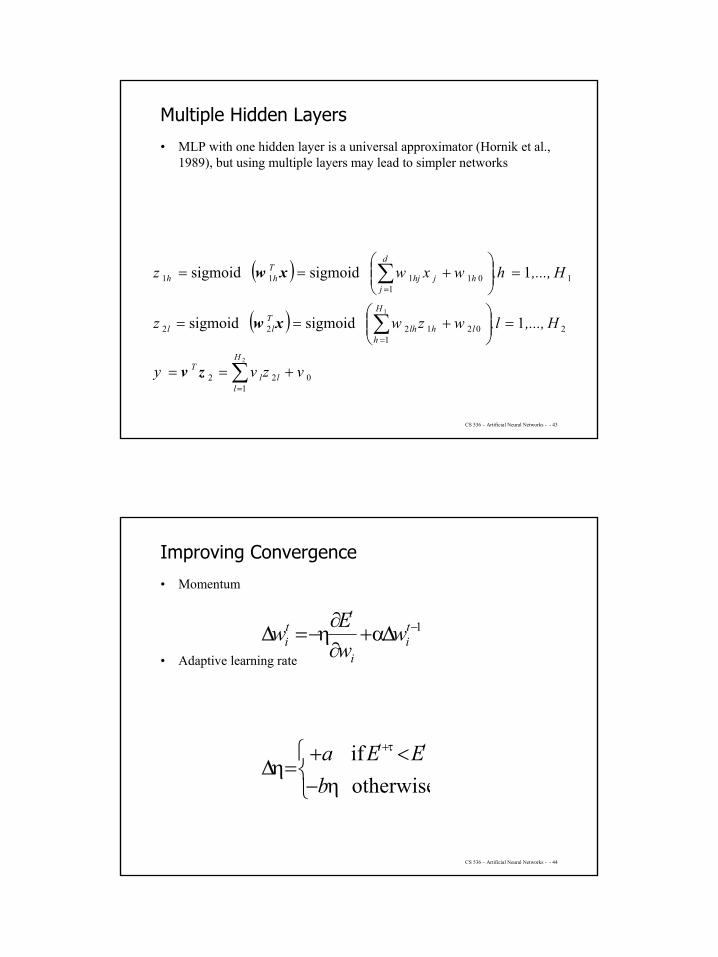
Multiple Hidden Layers
• MLP with one hidden layer is a universal approximator (Hornik et al., 1989), but using multiple layers may lead to simpler networks
( )
( )
∑
∑
∑
=
=
=
+==
=
+==
=
+==
2
1
1022
21
021222
11
01111
1sigmoidsigmoid
1sigmoidsigmoid
H
lll
T
H
hlhlh
Tll
d
jhjhj
Thh
vzvy
H,...,l,wzwz
H,...,h,wxwz
zv
xw
xw
CS 536 – Artificial Neural Networks - - 44
Improving Convergence
• Momentum
• Adaptive learning rate
1−α+∂∂
η−= ti
i
tti w
wEw ∆∆
η−<+
=ητ+
otherwiseif
bEEa tt
∆
23
CS 536 – Artificial Neural Networks - - 45
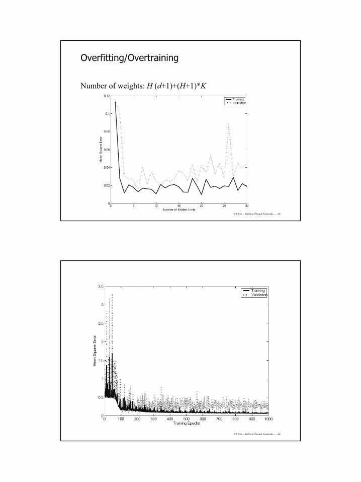
Overfitting/Overtraining
Number of weights: H (d+1)+(H+1)*K
CS 536 – Artificial Neural Networks - - 46
24
CS 536 – Artificial Neural Networks - - 47
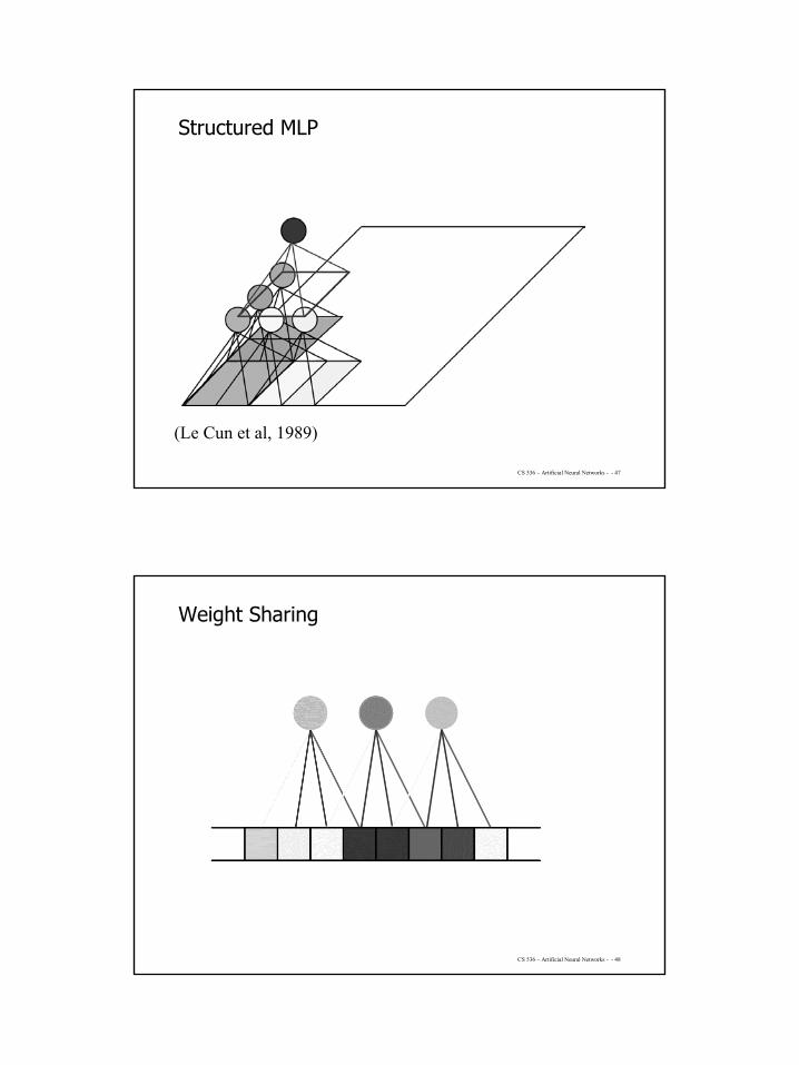
Structured MLP
(Le Cun et al, 1989)
CS 536 – Artificial Neural Networks - - 48
Weight Sharing

25
CS 536 – Artificial Neural Networks - - 49
Convolutional neural networks• Also known as gradient-based learning• Template matching using NN classifiers seems to work• Natural features are filter outputs
– probably, spots and bars, as in texture– but why not learn the filter kernels, too?
• a perceptron approximates convolution.• Network architecture: Two types of layers
– Convolution layers: convolving the image with filter kernels to obtain filter maps– Subsampling layers: reduce the resolution of the filter maps– The number of filter maps increases as the resolution decreases
CS 536 – Artificial Neural Networks - - 50
Figure from “Gradient-Based Learning Applied to Document Recognition”, Y. Lecun et al Proc. IEEE, 1998 copyright 1998, IEEE
A convolutional neural network, LeNet; the layers filter, subsample, filter,subsample, and finally classify based on outputs of this process.
26
CS 536 – Artificial Neural Networks - - 51
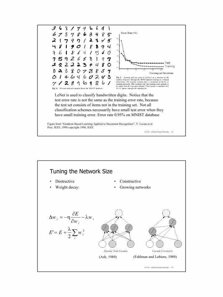
LeNet is used to classify handwritten digits. Notice that the test error rate is not the same as the training error rate, becausethe test set consists of items not in the training set. Not allclassification schemes necessarily have small test error when theyhave small training error. Error rate 0.95% on MNIST database
Figure from “Gradient-Based Learning Applied to Document Recognition”, Y. Lecun et al Proc. IEEE, 1998 copyright 1998, IEEE
CS 536 – Artificial Neural Networks - - 53
Tuning the Network Size
• Destructive• Weight decay:
• Constructive• Growing networks
(Ash, 1989) (Fahlman and Lebiere, 1989)
∑λ+=
λ−∂∂
η−=
ii
ii
i
wE'E
wwEw
2
2
∆

27
CS 536 – Artificial Neural Networks - - 54
Bayesian Learning
• Consider weights wi as random vars, prior p(wi)
• Weight decay, ridge regression, regularizationcost=data-misfit + λ complexity
( ) ( ) ( )( ) ( )
( ) ( ) ( )
( ) ( ) ( )
2
2
'
)2/1(2exp where
log|log|log
|log max argˆ ||
w
w
www
ww
wwww
λ
λ
+=
−⋅==
++=
==
∏
EE
wcwpwpp
Cppp
pp
ppp
ii
ii
MAP
XX
XX
XX
CS 536 – Artificial Neural Networks - - 55
Dimensionality Reduction

28
CS 536 – Artificial Neural Networks - - 56
CS 536 – Artificial Neural Networks - - 57
Learning Time
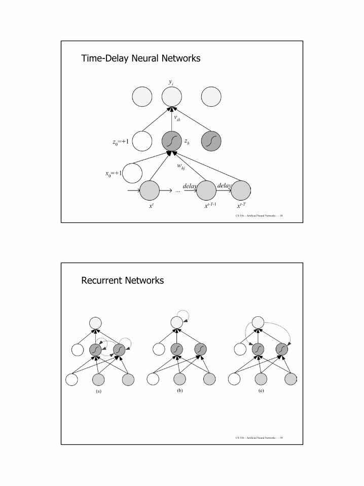
• Applications:– Sequence recognition: Speech recognition– Sequence reproduction: Time-series prediction– Sequence association
• Network architectures– Time-delay networks (Waibel et al., 1989)– Recurrent networks (Rumelhart et al., 1986)
29
CS 536 – Artificial Neural Networks - - 58
Time-Delay Neural Networks
CS 536 – Artificial Neural Networks - - 59
Recurrent Networks
30
CS 536 – Artificial Neural Networks - - 60
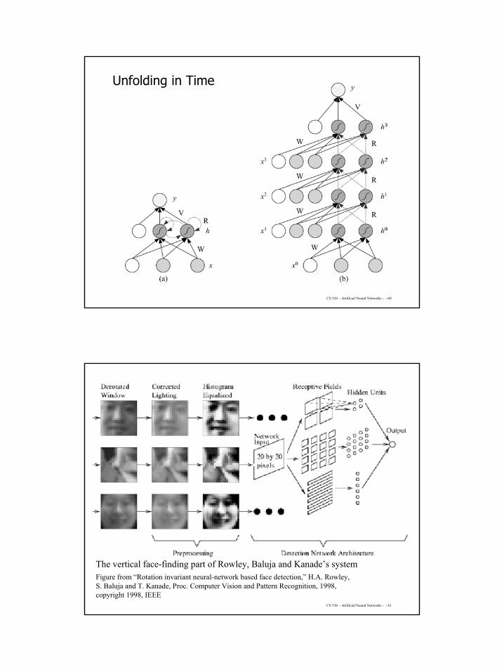
Unfolding in Time
CS 536 – Artificial Neural Networks - - 61
The vertical face-finding part of Rowley, Baluja and Kanade’s systemFigure from “Rotation invariant neural-network based face detection,” H.A. Rowley, S. Baluja and T. Kanade, Proc. Computer Vision and Pattern Recognition, 1998, copyright 1998, IEEE
31
CS 536 – Artificial Neural Networks - - 62
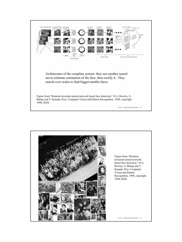
Architecture of the complete system: they use another neuralnet to estimate orientation of the face, then rectify it. They search over scales to find bigger/smaller faces.
Figure from “Rotation invariant neural-network based face detection,” H.A. Rowley, S. Baluja and T. Kanade, Proc. Computer Vision and Pattern Recognition, 1998, copyright1998, IEEE
CS 536 – Artificial Neural Networks - - 63
Figure from “Rotation invariant neural-network based face detection,” H.A. Rowley, S. Baluja and T. Kanade, Proc. Computer Vision and Pattern Recognition, 1998, copyright 1998, IEEE

32
CS 536 – Artificial Neural Networks - - 64
Sources
• Slides by Ethem Elpaydin, “introduction to machine learning” © The MIT Press, 2004
• Slides by Tom M. Mitchell• Ethem Elpaydin, “introduction to machine learning” Chapter 10• Tom M. Mitchell “Machine Learning”


![Deep Parametric Continuous Convolutional Neural Networks€¦ · Graph Neural Networks: Graph neural networks (GNNs) [25] are generalizations of neural networks to graph structured](https://static.fdocuments.in/doc/165x107/5f7096c356401635d36dbe30/deep-parametric-continuous-convolutional-neural-networks-graph-neural-networks.jpg)