Nova Southeastern University Nova Southeastern University

NSUWorks NSUWorks

CCE Theses and Dissertations College of Computing and Engineering

2021

Neural Network Variations for Time Series Forecasting Neural Network Variations for Time Series Forecasting

David Ason Nova Southeastern University, dave.ason@gmail.com

Follow this and additional works at: https://nsuworks.nova.edu/gscis_etd

Part of the Computer Sciences Commons

Share Feedback About This Item

NSUWorks Citation NSUWorks Citation David Ason. 2021. Neural Network Variations for Time Series Forecasting. Doctoral dissertation. Nova Southeastern University. Retrieved from NSUWorks, College of Computing and Engineering. (1150) https://nsuworks.nova.edu/gscis_etd/1150.

This Dissertation is brought to you by the College of Computing and Engineering at NSUWorks. It has been accepted for inclusion in CCE Theses and Dissertations by an authorized administrator of NSUWorks. For more information, please contact nsuworks@nova.edu.

Neural Network Variations for Time Series Forecasting

by

David Ason

A dissertation submitted in partial fulfillment of the requirements

for the degree of Doctor of Philosophy

in

Computer Science

College of Computing and Engineering

Nova Southeastern University

2021

An Abstract of a Dissertation Submitted to Nova Southeastern University in Partial Fulfillment

of the Requirements for the Degree of Doctor of Philosophy

Neural Network Variations for Time Series Forecasting

by

David Ason

2021

Time series forecasting is an area of research within the discipline of machine learning. The

ARIMA model is a well-known approach to this challenge. However, simple models such as

ARIMA do not take into consideration complex relationships within the data and quite often fail

to produce a satisfactory forecast. Neural networks have been presented in previous works as an

alternative. Neural networks are able to capture non-linear relationships within the data and can

deliver an improved forecast when compared to ARIMA models.

This dissertation takes neural network variations and applies them to a group of time series

datasets found in the literature to look for forecasting improvements and generalizability. Metrics

used to compare the effectiveness of the variations will be taken from the literature and include

the Root Mean Squared Error (RMSE), Directional Accuracy (DA), and Mean Absolute

Percentage Error (MAPE).

A total of 12 datasets were used for this study: 6 series each with a daily and weekly version.

Analysis of the results demonstrates that it is possible to improve performance as gauged by the

metrics in most instances. Neural networks with a feature detection component such as a

convolutional layer or a temporal component such as RNN variations are effective when scored

by the directional accuracy metric. Convolutional layers appear to be especially effective at the

weekly level of granularity in this study. The Stacked Denoising Autoencoder (SDAE)

performed well when judged by the RMSE and MAPE metrics.

The directional accuracy metric was further broken down into a classification problem:

precision, recall, and F1 metrics were used for this evaluation. In addition, the research included

evaluating the models’ ability to predict multiple steps ahead: steps t+1, t+2, and t+3 were

examined. The predictive power of the models generally decreased as timesteps increased. RNN

variations continued to do well at timesteps beyond t+1 for directional accuracy. The predictive

power of the SDAE held up well beyond the t+1 step and dominated the MAPE and RMSE

metrics at steps t+2 and t+3.

Acknowledgements

I would like to start by thanking the faculty and staff at Nova Southeastern University’s

College of Computing and Engineering for giving me the opportunity to pursue a long-held

dream of completing a Doctor of Philosophy degree in Computer Science. The classes that

comprised the core curriculum were engaging and interesting. They helped shape my

understanding of what research would entail. In particular, I would like to express my gratitude

to:

• Dr. Sumitra Mukherjee, my dissertation chair, for his advice, feedback, and the

benefit of his wisdom and experience. My dissertation topic was conceived during his

Artificial Intelligence class, and my work would not have been possible without his

support.

• Dr. Francisco Mitropoulos and Dr. Michael Laszlo for participating on my

dissertation committee and providing excellent instruction in the core classes I took

with them.

Lastly, I would like to thank my family for their support and love as I pursued my

passion. It would not have been possible without them.

iii

Table of Contents List of Figures .............................................................................................................. vii

List of Tables............................................................................................................... viii

Chapter 1 Introduction .....................................................................................................1

Problem Statement .......................................................................................................2

Dissertation Goal .........................................................................................................3

Research Questions ......................................................................................................4

Relevance and Significance .........................................................................................4

The Random Walk Model ........................................................................................4

The ARIMA Model .................................................................................................5

Long Short Term Memory Neural Networks ............................................................7

The Gated Recurrent Unit ........................................................................................9

Ensembling ............................................................................................................ 10

Barriers and Issues ..................................................................................................... 10

Assumptions, Limitations, and Delimitations ............................................................. 11

Definition of Terms ................................................................................................... 12

Summary ................................................................................................................... 12

Chapter 2 Review of the Literature ................................................................................ 14

Introduction ............................................................................................................... 14

iv

The Challenge of Time Series Forecasts .................................................................... 14

A Review of Approaches to Time Series Forecasting ................................................. 15

Time Series Forecasting with Convolutional Neural Networks ............................... 15

Time Series Forecasting with Recurrent Neural Networks ...................................... 18

Time Series Forecasting with Stacked Autoencoders .............................................. 22

Ensembling Multiple Models to Improve Prediction .............................................. 25

Summary ................................................................................................................... 26

Chapter 3 Methodology ................................................................................................. 27

The Datasets .............................................................................................................. 27

Create Baseline Prediction Models............................................................................. 28

Create the SDAE Model ............................................................................................ 29

Create Neural Network Variations ............................................................................. 29

Long Short Term Memory Neural Networks .......................................................... 29

Gated Recurrent Unit Neural Networks .................................................................. 30

Convolutional Neural Networks ............................................................................. 31

Hybrid Model Variations ....................................................................................... 32

Model Tuning ............................................................................................................ 34

Random Hyperparameter Search ............................................................................ 35

Optimized Hyperparameter Search ......................................................................... 36

Use Ensembling to Improve Model Prediction Results ............................................... 38

v

Compare the Models Using Performance Evaluation Metrics ..................................... 39

Data Analysis......................................................................................................... 40

Format for Presenting Results ................................................................................ 41

Resources .................................................................................................................. 43

Summary ................................................................................................................... 44

Chapter 4 Results ........................................................................................................... 45

Introduction ............................................................................................................... 45

Data Analysis ............................................................................................................ 46

SDAE and baseline comparisons ............................................................................ 47

SDAE and Baselines on Other Datasets ................................................................. 49

Looking for improvement beyond the baselines ..................................................... 51

Ensembling ............................................................................................................ 59

Directional Accuracy ............................................................................................. 64

Directional Accuracy Summary ............................................................................. 73

k-ahead Predictions ................................................................................................ 73

k-head Prediction Summary ................................................................................... 79

Findings ..................................................................................................................... 80

Summary of Results ................................................................................................... 82

Chapter 5 Conclusions ................................................................................................... 84

Implications ............................................................................................................... 85

vi

Recommendations for Future Work ........................................................................... 86

Summary ................................................................................................................... 87

References ..................................................................................................................... 89

Appendix A ................................................................................................................... 92

Appendix B – Model Configurations ............................................................................. 93

vii

List of Figures

Figure 1: A GRU cell .................................................................................................................9

Figure 3: Pseudocode for a LSTM model ................................................................................. 29

Figure 4: Pseudocode for a GRU model.................................................................................... 30

Figure 5: Pseudocode for a CNN model ................................................................................... 31

Figure 6: stat-lstm architecture ................................................................................................. 33

Figure 7: cnn-lstm architecture ................................................................................................. 34

Figure 8: The SDAE model (red) compared with the t-1 value (green) and the actual WTI price

(black)....................................................................................................................................... 46

Figure 9: The SDAE model and baselines ................................................................................ 47

Figure 10: Sample LSTM model output on EURUSD .............................................................. 53

Figure 11: CNN model on USDJPY ......................................................................................... 55

Figure 12: Stat-LSTM model on the TNX index ....................................................................... 57

Figure 13: CNN-LSTM forecast on the VIX index ................................................................... 59

Figure 14: t+k ahead predictions ............................................................................................... 74

viii

List of Tables

Table 1: Sample model information .......................................................................................... 41

Table 2: Sample model parameters ........................................................................................... 43

Table 3: SDAE and benchmark comparisons on WTI data........................................................ 48

Table 4: SDAE and benchmarks on weekly data ....................................................................... 49

Table 5: SDAE and benchmark metrics for the daily timeframe................................................ 50

Table 6: LSTM and benchmark metrics for the weekly timeframe ............................................ 51

Table 7: LSTM and baselines for the daily timeframe ............................................................... 52

Table 8: CNN and baselines for the weekly timeframe ............................................................. 54

Table 9: CNN and baselines for the daily timeframe ................................................................. 54

Table 10: stat-lstm hybrid model and baselines on weekly data ................................................. 55

Table 11: stat-lstm hybrid model and baselines on daily data .................................................... 56

Table 12: cnn-lstm hybrid model and baselines on weekly data ................................................ 58

Table 13: cnn-lstm hybrid model and baselines on daily data .................................................... 58

Table 14: SDAE Ensembled values and their relative improvement .......................................... 60

Table 15: LSTM Ensembled values and their relative improvement .......................................... 61

Table 16: cnn ensembled values and their relative improvement ............................................... 62

Table 17: stat-LSTM ensemble results and their relative improvement ..................................... 63

Table 18: cnn-lstm ensemble results and their relative improvement ......................................... 64

Table 19: Precision, Recall, and F1 for EURJPY ...................................................................... 66

Table 20: Precision, Recall, and F1 for EURUSD ..................................................................... 67

Table 21: Precision, Recall, and F1 on USDJPY ....................................................................... 68

ix

Table 22: Precision, Recall, and F1 for the SPX ....................................................................... 69

Table 23: Precision, Recall, and F1 for the TNX ...................................................................... 71

Table 24: Precision, Recall, and F1 scores for the VIX ............................................................. 72

Table 25: t+k ahead prediction metrics for EURJPY ................................................................. 74

Table 26: t+k ahead predictions for EURUSD .......................................................................... 75

Table 27: t+k ahead predictions for USDJPY............................................................................ 76

Table 28: t+k ahead predictions for the SPX ............................................................................. 77

Table 29: t+k ahead predictions for the TNX ............................................................................ 78

Table 30: t+k ahead predictions for the VIX ............................................................................. 79

Table 31: Best model by category: mean of 10 runs .................................................................. 80

Table 32: Best ensembled model by category ........................................................................... 81

Table 33: CNN Configuration Parameters ................................................................................ 93

Table 34: CNN-LSTM Configuration Parameters ..................................................................... 94

Table 35: LSTM Configuration Settings ................................................................................... 95

Table 36: stat-lstm configuration parameters ............................................................................ 95

1

Chapter 1

Introduction

Forecasting time series data is a subject of interest in multiple fields. However,

forecasting is made difficult by complex relationships and non-linearity in the data (Borovykh,

Bohte, & Oosterlee, 2017). This complexity has led to different approaches to constructing

forecasting models.

Neural network variations such as Convolutional Neural Networks (CNNs), Long Short

Term Memory (LSTMs), and Gated Recurrent Units (GRUs) have been used for time series

forecasts in different domains. Convolutional Neural Networks (CNNs), originally developed to

learn features in an image, have been adapted to forecast time series data (Borovykh et al., 2017;

Mittlelman, 2015). Borovykh et al. (2017), note that there can be correlations between financial

time series. The authors seek to exploit these correlations by using multiple time series as input

to train a CNN (Borovykh et al., 2017). In Mittelman (2015), the author uses a variant CNN,

known as an Undecimated Fully Convolutional Neural Network (UFCNN) to generate forecasts

on three different time series datasets.

GRUs and LSTMs were compared to another neural network model as a way to predict

time series in the work by Chung, Gulcehre, Cho, and Bengio (2014). In their research, the

authors use voice and music data as time series sequences upon which to evaluate the neural

networks. The paper concludes by noting that GRUs show superior performance with some of

the test data, but with other data, the LSTM demonstrates better performance (Chung et al.,

2014). GRUs have also been used to infer missing data to improve time series predictions for

clinical data (Che, Purushotham, Cho, Sontag, and Liu, 2018).

2

Other forecast research seeks to combine neural network variations to improve forecast

accuracy. In Xingjian et al. (2015), the authors combine the convolutional layers of a CNN with

a LSTM to increase the accuracy of short-term weather forecasts. The authors use time series

radar map data to forecast future radar map behavior. The convolutional layer is used to learn

significant spatial features in the data which is then fed into the LSTM network. This

combination of models enables effective short-term weather forecasting, outperforming a LSTM

model and traditional forecast models (Xingjian et al., 2015).

Problem Statement

The Autoregressive Integrated Moving Average (ARIMA) model is a traditional and

popular forecasting tool (Kardakos et al., 2013). However, models such as ARIMA often fail to

make effective forecasts due to the complexity of the relationships in the data (Borovykh et al.,

2017). In Zhao, Li, and Yu (2017), the authors focus on using a neural network variant known as

a Stacked Denoising Autoencoder (SDAE) to predict the price of oil. However, forecasting a

time series such as crude oil or a stock price is challenging because of the nonlinearity, complex

dynamics, and potential non-stationarity of the data (Cao, Li, & Li, 2018; Zhang, Zhang, &

Zhang, 2015). Combinations such as this lead to a complex system whose mechanisms are not

well understood (Alvarez-Ramierz, Soriano, Cisneros, & Suarez, 2003).

In addition to the complex dynamics that make up a financial time series, a time series

itself is related to both data at the current time as well as data from earlier times. Information

from earlier times will be lost if only the present time is considered. Traditional neural networks

(ANNs) can fail to capture this without a mechanism to maintain state. Variant neural networks

such as recurrent neural networks (RNNs) have the ability maintain the state of recent time series

3

movement (Cao, et al., 2018). Because of the inherent complexity in time series data, an accurate

forecast is difficult (Boroyvkh et al., 2017).

Dissertation Goal

The primary goal of this research was to develop and evaluate improved neural network-

based models for time series forecasting. The models were compared to the ARIMA and random

walk models as baselines using benchmark datasets.

The Zhao (2017) dataset consists of WTI price data at the monthly level. Because of this

relatively coarse granularity, only 365 observations are available in this dataset. To facilitate as

accurate an assessment as possible, model variations were tested on datasets found in the

literature beyond the WTI data with more observations. These include the S&P 500 (SPX) broad

market index found in Wiese et al., (2020); an interest rate (TNX) and volatility (VIX) index

found in Borovykh et al., (2017); and the forex currency pairs Euro – Dollar (EURUSD), Dollar

– Japanese Yen (USDJPY), and the Euro – Japanese Yen (EURJPY) found in Mayo, M. (2012).

This study started by comparing the SDAE model against the baselines on the WTI

dataset. The SDAE and baselines were then run on the other time series to look for

generalizability. Next, neural network models such as the CNN, LSTM, and hybrid variants were

developed and evaluated against results produced by the SDAE and baselines.

Comparisons were based on the metrics that are used in Zhao et al. (2017): Root Mean

Squared Error (RMSE), Directional Accuracy (DA), and Mean Absolute Percentage Error

(MAPE). The precision, recall, and F1 scores as defined in Opitz & Burst (2019) were used to

analyze directional accuracy prediction. The goal was to develop models that perform better than

the ARIMA and random walk baselines on the datasets found in the literature.

4

Research Questions

The primary research question for this study is forecast accuracy: is it possible to improve

upon the results from the baselines on the selected datasets? An investigation was done into

neural network variations that included configuration variations such as the network depth,

number of neurons per hidden layer, and activation functions in an effort to improve upon the

forecast. The question posed was then answered with the use of metrics taken from the literature.

Relevance and Significance

Accurate time series predictions are difficult because of the non-linear relationships in the

data as well as noise. Common approaches to time series forecasting such as ARIMA models do

not capture the complex relationships effectively (Borovykh et al., 2017). This study used a

random walk and ARIMA model as baselines and compared them with neural network-based

approaches. The models used in this dissertation are briefly described next.

The Random Walk Model

The random walk model has been used as a baseline in previous studies (Mittlelman,

2015; Zhao et al., 2017). The random walk is described in Hyndman & Athanasopoulos (2018)

as forecasting the current value, 𝑦𝑡, as the value from the previous time, 𝑦𝑡−1, plus a white noise

or random element, 𝜀𝑡 . In equation form:

𝑦𝑡 = 𝑦𝑡−1 + 𝜀𝑡

(Hyndman & Athanasopoulos 2018).

5

The ARIMA Model

The ARIMA model is a simple and popular model for forecasting. Also known as the

Box-Jenkins method, it was originally described in their 1970 textbook, Time Series Analysis:

Forecasting and Control. The ARIMA model is defined in Hyndman & Athanasopoulos (2018)

as:

𝑦𝑡′ = c + 𝜙1𝑦𝑡−1

′ + …. + 𝜙𝑝𝑦𝑡−𝑝′ + 𝜀𝑡 + 𝜃1𝜀𝑡−1+ … + 𝜃𝑞𝜀𝑡−𝑞

In the ARIMA model the output 𝑦𝑡′ is the differenced series at time t, and the right-hand side of

the equation are predictors including lagged values of 𝑦𝑡 and lagged errors. Differencing is the

computation of the differences between sequential observations and can be used to stabilize a

time series’ mean (Hyndman & Athanasopoulos, 2018).

The equation to determine the output is specified in terms of the following:

c, 𝜙, and 𝜃 are parameters of the model to be estimated

𝜀𝑡 is noise or the error term

p is the order of the order of the autoregressive process

q is the order of the moving average

(Hyndman & Athanasopoulos, 2018)

Convolutional Neural Network

Convolutional Neural Networks have grown in popularity as an effective tool for image

recognition after the seminal paper by LeCun, Bottou, Bengio, and Haffner was published in

1998. In this paper, CNNs were introduced for pattern recognition problems such as speech or

handwriting. A CNN passes data through a convolutional layer containing feature maps to

extract features out of the data. The data is then sub-sampled to reduce the sensitivity to specific

6

inputs and is eventually passed into a fully connected layer (LeCun et al., 1998). A fully

connected network is one where each node (or neuron) is connected to all of the nodes in the

next layer.

A convolutional transform is a mathematical operation on the input data that learns to

recognize features within the data. A CNN has layers of convolution operations applied to the

input. The weights for the convolutions are learned through training on input data (Borovykh et

al., 2017).

The CNN’s ability to effectively extract features and recognize patterns have been

adapted to the problem of time series forecasting (Borovykh et al., 2017; Mittelman, 2015). As

part of the adaption to time series forecasting, the shape of the convolutional operations is

modified to one dimension, along the sequence of input data. The convolutions operate on the

input data as a sliding window, moving across the input data and having the product of the

convolution filter and the data calculated. This process allows the model to learn features or

repeating patterns in the data. These abstract features and patterns are used to forecast future

values (Borovykh et al., 2017).

A max-pooling layer is used to make the input less subject to small variations and is a

common feature in many CNN implementations. However, for time series forecasting, this may

not be a desired feature (Mittelman, 2015).

Tunable parameters for the model include the number of convolutional filters, the size of

the filter, the number of layers in the neural network, the number of neurons in each layer, as

well as the activation function. Cross validation training on the input data is used to select or tune

the parameters (Mittelman, 2015).

7

Stacked Denoising Autoencoder

A neural network variant, known as a stacked denoising autoencoder (SDAE), is used as

the central algorithm in Zhao et al.’s 2017 research. The SDAE starts with an autoencoder, a

neural network that maps an input vector to a hidden representation of the input’s features. An

autoencoder is a neural network with one hidden layer where the length of both the input and the

output are of the same size. There are two parts to an autoencoder: encoding to a hidden

representation, and then decoding to an output of the same length as the input. For input vector x

of length d, input x is mapped to a hidden representation y with the following function:

y = 𝑓𝜃

(𝑥) = 𝜙𝑓(𝑊𝑥 + b)

𝑓(𝑥) has as parameters W, a 𝑑′ ∗ 𝑑 weight matrix, b a bias vector, and 𝜙() a non-linear

activation function. The hidden representation is then translated back to vector z, a reconstruction

of input vector x:

z = 𝑔𝜃′

(𝑦) = 𝜙𝑔(𝑊′

y + 𝑏′)

where 𝑊′ is a weight matrix, 𝑏′

is a bias vector and 𝜙() is a non-linear activation

function.

In the variation known as a denoising autoencoder, noise is added to the input, so the

model learns to construct a clean representation of the corrupted input. The algorithm becomes

stacked as denoising autoencoders are layered in the model (Zhao et al., 2017; Vincent,

Larochelle, Lajoie, & Bengio, 2010).

Long Short Term Memory Neural Networks

Recurrent Neural Networks (RNNs) capture a time element in the data by maintaining a

current state within an individual neuron that is dependent upon a previous state. However, it is

8

noted in Chung et al.’s (2014) work that RNNs can be difficult to train using a traditional

backpropagation method because the gradient in the training algorithm can either vanish to zero

or grow without bound and explode (Chung et al., 2014).

The LSTM uses the concept of a memory cell, which uses gates to control the flow of

information to and from the cell (Hochreiter & Schmidhuber, 1997). The LSTM unit sums the

weighted input signals as a traditional neural network, but also applies a memory value c that is

controlled by a modulation function o:

ℎ𝑡𝑗 = 𝑜𝑡

𝑗 tanh (𝑐𝑡

𝑗 )

Where:

ℎ𝑡𝑗is the output of the activation function for an LSTM

𝑐𝑡𝑗 is memory at time t

𝑜𝑡𝑗 is the output gate that modulates the memory content exposure

j represents the j-th LSTM unit

(Chung et al., 2014)

The LSTM neural network architecture was developed by Hochreiter & Schmidhuber in

1997. The LSTM maintains state like an RNN but addresses the issue RNNs have with the

training gradient (Hochreiter & Schmidhuber, 1997). The cell structure characteristic of LSTMs

allows it to effectively model time series data with long time lags. In addition, testing has shown

LSTMs are able to handle noise in the data and can work well with different parameter settings

such as learning rates (Hochreiter & Schmidhuber, 1997).

9

The Gated Recurrent Unit

Gated Recurrent Units, GRUs, are based on RNNs but modify the activation function

with gating units, like the LSTM. GRUs have gating units to control the flow of information

within a cell but do not have separate memory cells. GRUs have been used for language

translation (Cho, Van Merrienboer, Bahdanau, and Bengio 2014a) and sequence prediction

(Chung et al., 2014). The gating mechanism found in GRUs is described in (Cho et al., 2014b).

The architecture of a GRU is influenced by the design of an LSTM but is simpler and

streamlined. The GRU architecture is as follows (Cho et al., 2014b):

Figure 1: A GRU cell

Where the activation of the jth hidden unit is computed as a function of the states above:

𝑟𝑗 = 𝜎 ([𝑊𝑟𝑥 ]𝑗 + [𝑈𝑟ℎ(𝑡−1) ]𝑗)

Where 𝜎 is a logistic sigmoid function.

[. ]𝑗is the jth element of a vector

x is the input and ℎ(𝑡−1) is the previous hidden state

𝑊𝑟 and 𝑈𝑟 are weight matrices which are learned through training

The update gate 𝑧𝑗is computed by:

𝑧𝑗 = 𝜎 ([𝑊𝑧𝑥 ]𝑗 + [𝑈𝑧ℎ(𝑡−1) ]𝑗)

(Cho et al., 2014b)

10

Ensembling

Ensembling is a technique used to improve model performance by creating a blended

prediction from multiple models. In Zhao et al.’s 2017 research on oil price forecasting, the

authors use an ensemble variation known as bagging. The final ensemble prediction is an

average of the individual models’ predictions (Breiman, L., 1996). By creating a composite

prediction with multiple models, it is possible to reduce overfitting (Goodfellow, Bengio, &

Courville, 2016). This study used ensembling as a method to look for further performance

improvement. Results with and without ensembling are presented in Chapter 4.

Barriers and Issues

Neural networks can require large datasets to obtain reliable results (Borovykh et al.,

2017). The Zhao dataset is relatively modest in size at 365 observations, each with 200 features.

The results obtained by the neural networks proposed for this study may be influenced by the

limited size of the dataset. When the number of features in a dataset, p, approaches the number of

rows, n, there is risk in overfitting the data when training a model (James et al., 2013).

Overfitting can happen if the features are perfectly correlated to the response variable or

if there is no correlation to the response variable. A good way to guard against this is to use a

hold out or test set for model validation (James et al., 2013). However, even when a test set is

used, certain metrics such as 𝑅2 will increase as the number of features in a model increases, so

care is warranted when judging the fitness of a particular model with a large number of features

in comparison to the number of observations (James et al., 2013).

The possibility exists that there still may be a coincidental correlation between the model

and the data. In Bao et al. (2017), the authors express concern over the success of models trained

on financial data being due to a coincidental correlation with data, rather than the power of the

11

model itself. To reduce the likelihood of this being the case, and to prove the robustness of their

results, the authors test their model on 6 different financial series (Bao et al., 2017). In order to

mitigate the risk of overfitting to a dataset that is limited in size, this study also used 6 different

time series and focused on two levels of granularity: the daily and weekly levels for a total of 12

datasets to be analyzed.

Another issue is hardware capacity. The limitation of the hardware capabilities selected

for this study imposes an upper bound on the size of the models that can be trained for the study.

Dean et al. (2012) notes that models can grow so large as to not fit in a single computer’s

memory. To help mitigate this risk, in addition to the local hardware used, models were also

trained using Google’s Collaboratory.

Assumptions, Limitations, and Delimitations

Development environment: Python was selected as the programming language since it is

a common language used for neural network development. The Keras library was also selected

for similar reasons: it is a popular choice for specifying neural network architectures.

Resources: the resources used for this project include a laptop and workstation. The

laptop has a 4 core Intel i7 processor, 16GB of RAM, and an nVidia GeForce GTX 960M

graphics card. The workstation has an 8 core AMD FX 8530 processor, 16GB of RAM, and an

nVidia GeForce GTX 650 graphics card. To facilitate the research, Google’s Collaboratory was

also used to train models.

12

Definition of Terms

ANN: Artificial Neural Network

ARIMA: Auto regressive integrated moving average, a method for time series

forecasting.

Back-propagation: an algorithm that works to minimize the error of a model through

repeated iterations of training. This is a time consuming and resource intensive process.

Ensembling: combining the output of more than one model to improve prediction

accuracy.

CNN: Convolutional Neural Network.

Epoch: during model training, an iteration where the entire training set is presented to the

model one time.

GPU: Graphics Processing Unit.

GRU: Gated Recurrent Unit, a variant RNN.

LSTM: Long Short-Term Neural Network, a variant RNN.

RNN: Recurrent Neural Network.

SDAE: Stacked Denoising Autoencoder, a neural network variation.

WTI: West Texas Intermediate, a tradable crude oil commodity

Summary

Time series forecasts are made difficult due to nonlinearity and complex relationships in

the data. Several neural network variations have been applied to the challenge of time series

forecasting. Convolutional Neural Networks, developed for image recognition, have been

successfully applied to time series data (Borovykh et al., 2017; Mittlelman, 2015). Recurrent

13

neural network variations such as LTSMs and GRUs have memory cells and provide a temporal

factor in model training (Chung et al., 2014).

This study’s goal was to improve upon the forecast model baselines, ARIMA and random

walk, by examining neural network variations across different datasets. Methods of evaluating

the quality of model prediction includes metrics used in Zhao et al.’s (2017) work as well as

metrics to evaluate directional accuracy as a classification problem.

14

Chapter 2

Review of the Literature

Introduction

The purpose of this literature review is to expand upon the motivation for the proposed

research. The literature review is divided into three main parts. The first section will discuss the

challenge of time series forecasting. The second section reviews different approaches to time

series forecasting, concluding with a third section on ensembling as a way to improve model

accuracy.

The Challenge of Time Series Forecasts

Accuracy with time series forecasts is made difficult by the non-linearity of the data. In

addition, there is quite often a significant amount of noise in the data that further contributes to

the difficulty, making temporal relationships within the data hard to discern (Borovykh et al.,

2017). A good model will need to be robust and resistant to the noise in the data. With financial

data, the difficulty is increased because conditions change over time, limiting the utility of long

periods of data. (Borovykh et al., 2017).

Financial markets are highly unpredictable because of their characteristic high volatility.

The influences on the financial markets can be classified into two broad categories: macro and

micro variables. Macro variables include things like economic policy and the gross national

product (Zhou et al., 2016). Financial series such as the price of oil have been shown to be

correlated with the gross domestic product growth rate (Mostafa & El-Masry, 2016). By contrast,

micro variables are things like events, rumors, and the irrationality of investors (Zhou et al.,

15

2016). These influences combine to create non-linear behavior in the financial markets (Zhou et

al., 2016). Some financial series will alternate between periods of high and low volatility

(Morana, 2001). This volatility can add to the difficulty of an effective price forecast (Mostafa &

El-Masry, 2016). Time series models such as ARIMA often fail to capture the complexity of

financial markets (Zhou et al., 2016).

There is also a debate on whether financial markets are themselves predictable. The idea

of the Efficient Market hypothesis was first proposed in Malkiel & Fama (1970), stating that

current prices reflect all known information and so it is impossible to get an edge with a

forecasting technique (Nelson et al., 2017). However subsequent work has shown that there is

reason to question this hypothesis (Lo & MacKinlay, 2011; Nelson et al., 2017).

A Review of Approaches to Time Series Forecasting

Given the complexity of creating an accurate time series forecast, different variations of

neural networks have been proposed to improve forecast reliability. This section reviews neural

network variations and provides an overview of how they are used to address time series.

Time Series Forecasting with Convolutional Neural Networks

CNNs, originally developed for image recognition, have been adapted to time series

forecasting. A defining feature of the CNN is the convolutional layer, which consists of

mathematical operations that are applied to the input along a sliding window. This allows the

model to learn significant features or patterns within the input data. These patterns can then be

used to forecast future values (Borovykh et al., 2017).

16

In Borovykh et al. (2017), the authors use the concept of a dilated convolution to capture

long term dependencies. A dilated convolution has a dilation factor, d, where the model applies

the convolutional transform to every dth element in the input. This approach to convolutions

allows the model to learn dependencies farther apart than would otherwise be the case. Multiple

dilated convolutions are stacked in layers, with the dilation factors increasing according to a

power of 2. Part of the transformations include the wavelet transforms which seek to match a

function’s changes to a periodic wavelet function (Borovykh et al., 2017).

The structure of the neural network layer is common to other CNNs where, rather than

the neurons being fully connected between layers; neurons are instead locally connected to

regions within the input. This allows the CNN to learn features within the input. The

convolutions, wavelet transforms, and locally connected neural network combine to create the

WaveNet architecture used in the research (Borovykh et al., 2017).

The authors use multiple correlated time series as features for the input data with the aim

of leveraging the correlations to generate a better forecast. The model will then use the history of

the time series to be predicted as well as the related time series to learn relationships and features

within the data. This strategy is adopted to reduce noise within the data and improve the

robustness of the forecast. The data used for the research is the S&P 500 data, the volatility

index, as well a 10-year interest rate index (Borovykh et al., 2017). To test the performance of

the model, the authors attempt to forecast the day head value of the S&P 500. In addition, the

model architecture is tested on a combination of several Forex exchange rates to exploit the

patterns between currency pairs (Borovykh, et al., 2017). The authors divide the data into a

training period of 750 days and a test period of 250 days. The test data is used for the day ahead

17

predictions. The range of the data is from 01-01-2005 to 12-31-2016 and is split into nine periods

where the test data does not overlap with the training data (Borovykh et al., 2017).

Results of the CNN model plus the WaveNet transform compare favorably to the LSTM

architecture used as a baseline. Training time for the CNN model was faster than the LSTM

baseline (Borovykh et al., 2017).

When used for image processing, CNNs typically use a pooling layer between

convolutional layers to reduce the size of the input to the neural network. For time series, the

pooling layer can cause a loss of information and impact forecasting (Mittleman, R., 2015). In

Mittleman (2015), the author proposes an undecimated fully convolutional network (UFCNN)

where the input and output of the model have the same dimensions. Wavelet transforms are also

used in this research as part of a deconvolutional stage to match the input and output dimensions.

The UFCNN is based on a Fully Convolutional Network (FCN). The FCN uses max-

pooling layers characteristic of CNNs as a downsampling operation. The convolutions plus max-

pooling operations are used so that features within the data are learned, but the dimensions of the

input are preserved in the output of with upsampling operations that pad the data with zeros

(Mittleman, R., 2015). The UFCNN in Mittleman (2015) takes a different approach to

upsampling and downsampling. Instead of padding the data, the UFCNN takes inspiration from

wavelet transforms which are used so that filters at the different levels have corresponding

upsampling operations (Mittleman, R., 2015).

The UFCNN in Mittleman (2015) was tested on music datasets and high frequency

trading data. The music data includes the MUSE and NOTTINGHAM datasets consisting of an

88-dimension vector where each dimension is a musical note. The UFCNN was trained to

18

forecast the vector at the next timestep. To judge the effectiveness of the new model on the

music dataset, the mean squared error metric is used. When the Middleman (2015) UFCNN was

compared to an FCN, the UFCNN demonstrated better performance. When compared to the

RNN and LSTM baselines, the UFCNN outperformed both (Mittleman, R., 2015)

The high frequency trading data was obtained from the Circulum Vite site which

sponsors machine learning competitions on financial data. The financial data includes price and

volume plus other information sampled at two to three times per second, over a period of one

year. The data was partitioned into approximately eight months of training data, two months of

validation data, and two months of test data (Mittleman, R., 2015). The UFCNN algorithm was

trained as a classifier to predict at each time step whether the best action was to buy, sell or do

nothing. To judge the effectiveness of the model, the metrics of profit per time step and

classification accuracy are used. Other models used in the comparison include an RNN, a

random approach, and the Viterbi algorithm which sees the entire dataset and is used as a best

case upper bound for performance. The UFCNN outperformed both the random model and RNN

in both the profit per time step, and classification accuracy metrics (Mittleman, R., 2015).

Time Series Forecasting with Recurrent Neural Networks

RNNs are neural networks that maintain state and so are candidate architectures for

sequence and time series prediction. However, when trained, they suffer from issues with the

training gradient. A variation on RNNs, LSTMs, also maintain state, but do not suffer from

training gradient problems (Hochreiter & Schmidhuber, 1997).

In Nelson, Pereira, & Oliveira (2017), the LSTM is used to forecast a set of stocks from

the Brazilian market. The model in the study was designed as a classification model to predict an

19

up or down movement in a stock’s price. The data collected was from 2008 to 2015 at 15-minute

intervals. The difference of the logarithm function between timesteps was used as a transform to

stabilize the data series. In addition, 175 technical indicators were generated as features from the

price and volume of the stocks (Nelson et al., 2017).

The model in the study was trained on 10 months of data prior to a target day. The

previous week to the target day was used as an out of sample test set. The trained model was then

used to predict price movement for the following trading day. Each day a new model would be

trained for use on the following day. Metrics included for model evaluation were accuracy,

precision, recall, and the F1 score. The LSTM model was compared to a multi-layer perceptron,

the random forest, and a random model. The results of the study were very favorable to the

LSTM as a tool for time series forecasting (Nelson et al., 2017).

Another variation on the RNN is the Gated Recurrent Unit or GRU which has been

applied to the challenge of time series prediction. In Che et al. (2018), the authors use a GRU to

forecast mortality rates from healthcare data that contains missing values. The premise of the

study is that the patterns of missing data are itself information of a sort that can be leveraged as a

feature for the model. The authors create a new feature by looking at the missing data and

associating it with categorical values of other features including mortality and diagnosis. A

Pearson correlation was used to establish the statistical soundness of the association. It was

observed during the study that features with a low rate of missing values tended to have a high or

negative correlation with the labels of interest. The patterns of the missing data are then used as a

feature, rather than trying to impute the missing data prior to model construction. (Che et al.,

2018).

20

The model created in the study uses two features created with the missing data patterns: a

mask and time interval. The mask is a vector that denotes whether or not a feature is missing at a

given timestamp t. The mask is 1 if a feature is present, else it is 0. The time interval records the

number of timesteps since the last observation of a given feature. This allows the model to be

trained to recognize long term patterns as well as patterns within the missing data to make a

forecast (Che et al., 2018).

The authors name their model configuration GRU-D. This model is compared to other

models including support vector machines, random forests, and other GRU variations with

imputed values for missing data. GRU-D, by leveraging patterns in the missing data as a novel

feature, outperforms the other models. The authors note that their model is limited in that if there

is no pattern in the missing information, this will have a negative impact on model performance

(Che et al., 2018).

Convolutional Neural Networks and LSTMs have been combined as a way to improve

forecast accuracy. In Xingjian, Chen, Wang, & Yeung (2015), the authors seek to use a hybrid

CNN-LSTM model, known as ConvLSTM, as a way to predict short term weather events such as

rainfall intensity over a local region in a 0 to 6 hour time window. Predictions are made with past

radar map images, arranged in a series of timesteps, as a primary input. Each radar map is

represented as a matrix of M rows and N columns. Each pixel within this map is considered a

measurement. The radar images are arranged in a temporal order. This input then is used to

predict radar map images one or more timesteps into the future (Xingjian et al., 2015).

To gauge the effectiveness of their approach, Xingjian et al. (2015) compare their

ConvLSTM model against a Fully Connected LSTM (FC-LSTM) model on two datasets: a

21

synthetic dataset known as the Moving-MNIST dataset, and radar echo image data. With the

radar data, the ConvLSTM model is also compared to a conventional forecasting method known

as Real-time Optical flow by Variational methods for Echoes of Radar, or ROVER (Xingjian et

al., 2015). The FC-LSTM used in the authors’ research is based on an architecture used in

Srivastava, Mansimov, & Salakhudinov (2015) to predict video sequences. This study uses an

LSTM as an encoder to learn the representation of video sequences and then an LSTM decoder

to predict future sequences (Srivastava et al., 2015).

The Moving-MNIST dataset consists of 64 x 64 frames that contain a handwritten digit

that is moving around inside the frame. There are 10 frames for the input and 10 as output

(Xingjian et al., 2015). The radar echo dataset used in the research is a sample of radar data

collected in Hong Kong from 2011 to 2013. The radar data is sampled at the rate of once every 6

minutes. Because the authors are trying to predict rain patterns, they select the top 97 rainy days

during this period as their dataset. The radar images are cropped to the central 330 x 330 region

and converted to gray scale. The data is then further filtered so it becomes a 100 x 100 image

(Xingjian et al., 2015).

The ConvLSTM architecture consists of convolutional operations and LSTM nodes that

are stacked into one or more layers. The ConvLSTMs themselves may also be stacked. There are

two main parts to the structure: an encoding network and a forecasting network. The encoding

network learns a representation of the input and the forecasting network provides the prediction

(Xingjian et al., 2015).

When compared to the FC-LSTM, the proposed ConvLSTM outperforms the model

using a cross-entropy metric on the Moving-MNIST dataset. With the radar echo dataset, the

authors use several metrics for measuring the accuracy of a weather forecast, including the

22

rainfall mean squared error, critical success index, false alarm rate, probability of detection, and

correlation. The ConvLSTM outperforms both the FC-LSTM and the more conventional

ROVER forecasting method under all the rainfall metrics (Xingjian et al., 2015).

Time Series Forecasting with Stacked Autoencoders

An autoencoder is a neural network variation that seeks to learn a representation of the

input and then reconstruct the input as output. During training, a hidden layer learns features

within the data (Bao, Yue & Rao, 2017). In Zhao et al. (2017), the authors use a stacked

denoising autoencoder (SDAE) to forecast the price of crude oil. As described in the Relevance

and Significance section, a SDAE consists of more than one autoencoder stacked in layers. The

stacked autoencoder becomes denoising when noise is added to the input and trained against a

clean version of the data as a way to remove the noise (Zhao et al., 2017).

Zhao et al.’s (2017) work seeks to predict the price of West Texas Intermediate (WTI)

crude oil using a SDAE. To build a base dataset, the authors collect data from the Energy

Information Administration (EIA), the Federal Reserve Bank (FRB), and Yahoo! Finance. A

total of 198 features are gathered from these sources. Multiple related datasets are then created

from this base dataset using a technique known as bagging. Bagging, or bootstrap aggregation,

starts with a dataset of size N and creates new datasets also of size N by sampling with

replacement from the base dataset (Breiman., L. 1996).

The SDAE architecture is replicated, and multiple models are trained using the bagged

datasets. For prediction, the multiple models are used to generate a composite prediction with a

technique known as ensembling (Zhao et al., 2017). Ensembling leverages the predictive power

23

of multiple models to create a composite prediction that can have better performance than

individual models (Goodfellow et al., 2016).

To judge the effectiveness of this technique, the authors compare their model to several

other forecast models including a random walk, MRS (Markov Regime Switching), FNN

(Feedforward Neural Network), and a Support Vector Machine (SVR). The FNN and SVR are

also ensembled on a bagged dataset for comparison. The comparison of the models includes

metrics for prediction accuracy and statistical methods to test the model validity.

The metrics for prediction accuracy include directional accuracy, root mean squared error

(RMSE), and mean absolute percentage error (MAPE) (Zhao et al., 2017). Statistical methods

used to analyze the proposed method include the Wilcoxon signed rank test, the forecast

encompassing test, and the reality check. The Wilcoxon signed rank test is used to compare two

datasets that do not have to be normally distributed (Devore, J.L., 2011). The forecast

encompassing test is used to see if there is a statistically significant difference in the results of

the models (Harvey et al., 1998). Finally, the reality check looks for a false positive: given a

single dataset, if enough models are used to predict on it, there is the possibility of a model

showing a favorable result due to chance (White, H., 2000).

In Bao et al.’s (2017) publication, the researchers combine a wavelet transform, and two

neural networks: a stacked autoencoder and a LSTM network. Together, these components are

placed in a pipeline to create a composite model that is referred to as a WSAEs-LSTM (Bao et

al., 2017).

To generate a prediction, data is first passed through a wavelet transform as a way to

stabilize an irregular series such as financial data. Next, the data is passed through an

24

autoencoder in order to detect significant features. The data is then passed into a LSTM network

to generate a prediction (Bao et al., 2017).

This composite model is used to forecast the price of six separate stock market indices

including the Chinese CSI 300, the Indian Nifty 50, the Hang Seng from Hong Kong, Toyko’s

Nikkei 225, and the S&P 500 and Dow Jones Industrial Average from the United States. The

authors tested their novel architecture in multiple markets in order to see how well their model

would generalize across different time series. The authors sought indices from markets that can

be considered developing, developed, and a middle ground between the two in an effort to test

the robustness of their model (Bao et al., 2017).

To evaluate their model’s accuracy, Bao et al. (2017) used three primary metrics: MAPE,

the R correlation coefficient, and Theil’s inequality coefficient (Bao et al., 2017). Other models

were used as a basis for comparison to the WSAEs-LSTM; these include an RNN for a

performance benchmark, a LSTM, and a combination of wavelet transform and LSTM known as

the WLSTM. This last model was used to validate the efficacy of including an autoencoder as a

method of learning features in the data. The autoencoder as a means of learning features within

the data is what the authors view as their main contribution (Bao et al., 2017).

The study concluded by noting that their WSAEs-LSTM outperformed the other models

included in the study using all three of the aforementioned metrics. In addition, the authors note

that the models showed a correlation between the magnitude of their errors when the results were

compared by similar market development state. For example, the WSAE-LSTM had similar

errors when the S&P 500 and Dow index were measured, but the difference between the errors

was greater when the results of the S&P 500 and CSI 300 were compared (Bao et al., 2017).

25

Ensembling Multiple Models to Improve Prediction

In Zhao et al. (2017), ensembling is used to combine multiple independent model

predictions to increase the accuracy of a prediction. Ensembling a set of models can provide

more robust performance on out of sample data than a single model. While the most accurate

model in a set may outperform its ensemble, risk of using a poorly performing model on out of

sample data is reduced when an average prediction is taken (Polikar, R., 2006).

Ensembling is also a way to generate a composite prediction when the data is too large or

too complex to be accurately represented by a single model. For example, if the features are

radically different, such as a mix of image data, text data, and time series data, it is unlikely that

a single model can be trained to learn all of the features within the data (Polikar, R., 2006).

However, in such instances, it is possible to train a model on each class of data, and then

generate a composite prediction through ensembling. This is an example of data fusion (Polikar,

R., 2006).

Because of the noise and complexity inherent in most datasets, building a model with

perfect prediction accuracy is not realistic. However, it is possible to build a model that is correct

most of the time. With ensembling, the performance of such a model can be improved by adding

it to a group of other models (Polikar, R., 2006). To generate different models from a single

dataset, it is possible to use bagging, creating a new dataset from the original dataset by sampling

with replacement (Polikar, R., 2006; Zhao et al., 2017).

In Opitz & Maclin (1999), the researchers conducted an empirical study of ensembling

methods. The authors found that good ensembles are created when the models that compose the

ensemble make errors on different parts of the input. Citing earlier research, the authors state that

26

the best ensembles are composed of accurate models that otherwise disagree as much as possible

(Opitz & Maclin, 1999). One approach to having diverse but accurate models is to separate the

input into subtasks and then train models on these subtasks. These models are then combined

with a gating method to create a composite prediction (Opitz & Maclin, 1999).

Opitz & Maclin (1999) compare two variations on ensembling: bagging and boosting.

While bagging is generating a new dataset by sampling the original dataset with replacement,

boosting trains models serially where the training set of the next model is selected based on the

errors in the previous classifiers. Observations that the models have performed poorly on are

given more weight for new model training iterations. By doing this, boosting attempts to build

new models that strengthen currently poor performing areas (Opitz & Maclin, 1999).

The authors examine two forms of boosting, Arcing and Ada-boost, in addition to

bagging (Opitz & Maclin, 1999). The research demonstrated that bagging and boosting will

improve prediction results in most circumstances, when compared to a single model. However,

the authors note that in some instances boosting led to overfitting of the data by providing too

much weight to observations that were in actuality noise. In these instances, boosting hurt

accuracy (Opitz & Maclin, 1999).

Summary

This section started with a discussion of the challenges of time series forecasting: the

complex relationships in the data are hard to model. After the problem was introduced, the

literature review went into detail about different approaches to effectively modeling time series

data and using ensembling to improve model prediction. Chapter 3 will introduce the

methodology used in this study.

27

Chapter 3

Methodology

The goal of this dissertation was to develop and evaluate neural network-based models

for forecasting time series data, looking for improvements. This section describes the approach

that was taken to achieve this objective. Below is an outline of the steps that were taken as part

of the research. Each step will be expanded upon in turn:

1. Define the datasets

2. Create Random Walk and ARIMA models as a baseline

3. Create a SDAE model similar to Zhao et al. (2017)

4. Create neural network variations such as RNN variants, CNNs, and hybrid models then

compare them to extant methods on the selected time series

5. Model tuning

6. Use ensembling to improve model prediction

7. Compare the models using the performance analysis metrics

The Datasets

Zhao et al. (2017) focused their research on crude oil prices, specifically West Texas

Intermediate (WTI). The dataset consists of the monthly WTI price from January 1986 to May

2016. The data is sampled monthly for a total of 365 data points. There are 200 features in the

data including data related to crude oil production such as active rig count, road product

supplied, and aviation gasoline supplied. Financial indicators are also included as features. More

details about the dataset can be found in Appendix A. For Zhao et al.’s (2017) research, the first

28

80% of the data is used as a training set. The remaining 20% is used as test data. This dataset was

used for initial comparison of the SDAE model to the ARIMA and Random Walk baselines.

Because of the relatively limited number of observations available with the WTI and

related data, the study was broadened to compare the ARIMA and random walk baselines against

the SDAE and other neural networks on data found in the literature. This included a broad

market index, the SPX (Wiese et al., 2020; Borovykh et al., 2017), an interest rate (TNX) and

volatility index (VIX) (Borovykh et al., 2017) as well as the currency pairs EURUSD, EURJPY,

and USDJPY (Mayo, M., 2012). To facilitate a comparison with more observations, the daily

and weekly granularity was selected for each series bringing the total number of datasets to 12. A

total of 15 years of data was selected spanning the timeframe from 1/1/2005 to 1/1/2020. For the

weekly datasets, there are 783 observations per series. For the daily data, the observations vary

between 3740 and 4490 due to the different trading days of each series.

Zhao et al.’s (2017) research used 80% of the data for training and 20% of data as a test

set on which the metrics were calculated. This study took a similar approach, but varied the

proportions as follows: 70% of a dataset was used to train the model, 18% was used as a

validation set, and the remaining 12% was used as a test set to calculate model metrics. The

validation set was used to prevent overfitting. After each training epoch, the resulting model was

evaluated with the validation set using the loss function. If the model stopped improving based

on the validation set testing, training was ended. Metrics were then calculated on the test set.

Create Baseline Prediction Models

To determine the effectiveness of the models, baseline predictions were

generated. Several studies (Kaboudan, M.A, 2001; Morana, C., 2001; Mostafa & El-Masry,

29

2016; Zhao et al., 2017) use a random walk model as a baseline for comparison. Other research

uses the ARIMA model (Adhikari, R., 2015; Kardakos et al., 2013). Given their prevalence in

the literature, the random walk and ARIMA models were used as baselines in this study.

Create the SDAE Model

In the paper by Zhao et al. (2017), the architecture of the SDAE used in their

study is described. The model includes three hidden layers consisting of two Denoising

Autoencoders (DAEs) and a Feedfoward Neural Network (FNN). The number of neurons in each

layer are 200, 100, and 10, respectively. This study duplicated this structure to be used on each

dataset.

Create Neural Network Variations

Variations of neural networks were explored to look for improvements. This included

neural network variants such as CNNs, RNN variations, and hybrid models.

Long Short Term Memory Neural Networks

Given its success in previous forecast research, the LSTM was used in this study. The

LSTM model was built in Python using the Keras library for neural networks. The architecture

was similar to this pseudocode:

lstm = Sequential()

lstm.add(LSTM(units, input_shape(timesteps, feature_count)))

lstm.add(LSTM(units, activation=activation_type))

lstm.add(Dense(units, activation=activation_type))

lstm.compile(loss=loss_type, optimizer=optimizer_type, metrics = list_of_metrics)

Figure 2: Pseudocode for a LSTM model

30

The LSTM was tuned by adjusting the following parameters:

• The number of hidden layers

• The number of neurons per layer (‘units’ in the pseudocode above)

• The number of previous timesteps the model uses to make a prediction

(‘timesteps’ in the pseudocode)

• The activation function (‘activation_type’ in the pseudocode)

Gated Recurrent Unit Neural Networks

GRUs have been used for sequence prediction in works such as (Cho et al., 2014a; Chung

et al., 2014). Given their success with sequence prediction, they were used as part of the hybrid

models in this study.

Keras was also used for developing the GRUs. The models featuring GRUs were

constructed in a manner similar to the pseudocode below:

gru = Sequential()

gru.add(GRU(units, input_shape(timesteps, feature_count)))

gru.add(GRU(units, activation=activation_type))

gru.add(Dense(units, activation=activation_type))

gru.compile(loss=loss_type, optimizer=optimizer_type, metrics = list_of_metrics)

Figure 3: Pseudocode for a GRU model

In a manner similar to the LSTM, the GRU was tuned by adjusting the following

parameters:

• The number of hidden layers

• The number of neurons per layer (‘units’ in the pseudocode)

31

• The number of previous timesteps the model uses to make a prediction

(‘timesteps’ in the pseudocode)

• The activation function (‘activation_type’ in the pseudocode)

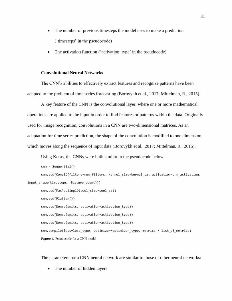
Convolutional Neural Networks

The CNN’s abilities to effectively extract features and recognize patterns have been

adapted to the problem of time series forecasting (Borovykh et al., 2017; Mittelman, R., 2015).

A key feature of the CNN is the convolutional layer, where one or more mathematical

operations are applied to the input in order to find features or patterns within the data. Originally

used for image recognition, convolutions in a CNN are two-dimensional matrices. As an

adaptation for time series prediction, the shape of the convolution is modified to one dimension,

which moves along the sequence of input data (Borovykh et al., 2017; Mittelman, R., 2015).

Using Keras, the CNNs were built similar to the pseudocode below:

cnn = Sequential()

cnn.add(Conv1D(filters=num_filters, kernel_size=kernel_sz, activation=cnn_activation,

input_shape(timesteps, feature_count)))

cnn.add(MaxPooling1D(pool_size=pool_sz))

cnn.add(Flatten())

cnn.add(Dense(units, activation=activation_type))

cnn.add(Dense(units, activation=activation_type))

cnn.add(Dense(units, activation=activation_type))

cnn.compile(loss=loss_type, optimizer=optimizer_type, metrics = list_of_metrics)

Figure 4: Pseudocode for a CNN model

The parameters for a CNN neural network are similar to those of other neural networks:

• The number of hidden layers

32

• The number of neurons per layer (‘units’ in the pseudocode)

• The number of previous timesteps the model uses to make a prediction

(‘timesteps’ in the pseudocode)

• The activation function (‘activation_type’ in the pseudocode)

In addition to the parameters common to other neural networks, CNNs will have the

following parameters for the convolutional layer that can be adjusted:

• The length of the convolutional filters (kernel_sz)

• The number of convolutional filters (num_filters)

• The activation function for the convolutional layer (cnn_activation)

Hybrid Model Variations

Hybrid models were also used in this study including the CNN-LSTM, and statistics-

LSTM variations.

As part of model tuning for the hybrid models, one of the hyperparameters was the neural

network type: LSTM or GRU.

Hybrid Model: Statistics – LSTM Model

Inspired by the Smyl (2020) paper describing the M4 competition winning algorithm, a

statistics-LSTM (or stat-LSTM) hybrid model was created to look for performance

improvements. However, the variation used in this research featured a level and seasonality

values that were chosen through hyperparameter optimization. The level and seasonality were

used as smoothing factors. Prior to the time series data being fed into the LSTM model as input,

the time series values were divided by the level and seasonality factors. As in Smyl’s (2020)

33

work, a logarithmic function was also applied as a preprocessing step. These steps were applied

in reverse order to unwind the preprocessing to obtain a final forecast value. As part of

hyperparameter tuning, the choice of RNN type: LSTM or GRU were variants that could be

selected.

Figure 5: stat-lstm architecture

CNN-LSTM Hybrid Model

Drawing inspiration from the Wavenet model in Borovykh et al. (2017), this work used

dilated convolutional layers as a way to detect features in the time series data and merged that

with the LSTM model network. The convolutional layers were a preprocessing step that served

34

to highlight significant features in the data prior to being fed into a LSTM model. As with the

stat-LSTM hybrid, as part of hyperparameter tuning, the choice of RNN type: LSTM or GRU

were variants that could be selected.

Figure 6: cnn-lstm architecture

Model Tuning

Most machine learning algorithms include configuration options known as

hyperparameters to adjust and optimize the functioning of the algorithm (Thornton, Hutter,

Hoos, & Leyton-Brown, 2013). Neural networks are no different. Typically, when applying a

machine learning algorithm to a problem, there are two selections that must be made: the

algorithm to be applied, and the configuration of the algorithm through hyperparameters. With

many models, there are a significant number of tunable parameters that create a large search

35

space. Finding the best configuration can be a daunting task. Using the default values can lead to

less than optimal results (Thornton et al., 2013). In the literature, methods of finding the best

parameter configuration range from an exhaustive grid search, random selection of

hyperparameter settings, to optimization algorithms (Bergstra & Bengio, 2012; Thornton et al.,

2013; van Stein, Wang, & Bäck, 2019).

Random Hyperparameter Search

A grid search through hyperparameter combinations is an exhaustive search through

every possible configuration combination. This has the advantage of being thorough but, is

subject to the curse of dimensionality as the number of possible combinations grows

exponentially with the number of possible hyperparameters (Bergstra & Bengio, 2012). With a

grid search, the size of the problem can be reduced by manually restricting the results to regions

in the space that appear to be promising, or by adjusting the resolution of the grid search so that

not every possible alternative is examined. This can make a prohibitively expensive grid search

tractable (Bergstra & Bengio, 2012). A more efficient alterative can be to use a random search

through the parameter space as an alternative to a grid search. Bergstra & Bengio (2012),

propose a random search that treats the configuration parameters as a uniform density from

which random samples are drawn. The authors state that this technique is a trade-off between

reduced efficiency in a low dimensional hyperparameter space with a significant improvement in

higher-dimensional spaces (Bergstra & Bengio, 2012).

In Bergstra & Bengio (2012), the authors conduct their comparison on several datasets

including the MNIST image classification dataset, variations on the MNIST dataset, and other

image classification datasets. A neural network is selected as the model with which to compare

the effectiveness of the hyperparameter optimization methods. The research concludes by noting

36

that not all hyperparameters are significant for a given machine learning problem, and which

hyperparameters are significant will change depending on the task. The grid search algorithm

spends too much time varying hyperparameters that are not significant. The paper concludes by

noting that random searches can find as good or better model configurations by searching a

larger space with a similar computational budget as a grid search. However, some manual

configuration by someone with expert domain knowledge combined with a grid search can beat

the proposed random search (Bergstra & Bengio, 2012).

Optimized Hyperparameter Search

In addition to a grid search and random search of the hyperparameter space, optimization

functions have been proposed as a means to find nominal model configurations (Thornton et al.,

2013; van Stein et al., 2019). In Thornton et al. (2013), the authors consider the problem of

model optimization to be a hierarchical search where the choice of the algorithm influences the

hyperparameters chosen, and subsequent inclusion of the model into an ensemble also impacts

any ensemble method hyperparameters. A Bayesian optimization method is proposed as an

alternative for selecting a good performance configuration for a given machine learning problem

(Thornton et al., 2013). The proposed Bayesian optimization method functions by iteratively

building models and then using the performance results from these models to find newer, and

hopefully better, hyperparameters with which to build a more accurate model. The authors use a

machine learning platform known as WEKA, an open source machine learning package, on

which to base their research (Thornton et al., 2013).

The hyperparameter optimization work proposed in Thornton et al. (2013), uses a total of

21 datasets on which to base their observations, which includes data from the UCI machine

learning repository, variations on the MNIST image classification dataset, and versions of the

37

CIFAR-10 datasets. The combination of a hyperparameter optimized search strategy along with

the WEKA toolkit is named Auto-WEKA by the authors (Thornton et al., 2013). The researchers

conclude their work by noting that their novel Auto-WEKA optimized parameter search

technique frequently outperforms other optimization methods on the 21 selected datasets

(Thornton et al., 2013).

In van Stein et al. (2019), the authors propose a method of effectively finding a nominal

configuration for convolutional neural networks through a parallel approach. The authors begin

by noting that while CNNs are very effective for image recognition and other machine learning

problems, most CNNs are configured by educated guess, a grid search, or by imitating a good

performance architecture from the literature (van Stein et al., 2019). As also documented in

(Bergstra & Bengio, 2012; Thornton et al., 2013), van Stein et al. (2019), note that the search

space for an optimized neural network configuration has a high dimensionality and there is a

correspondingly large number of hyperparameter combinations.

In addition to the large number of hyperparameter configurations, the computational

requirement for training a neural network is also significant. This can make it difficult to use

optimization approaches that may be suited for other machine learning algorithms (van Stein et

al., 2019). To establish a set of boundaries around the problem, the authors use a generic neural

network architecture that is very configurable as a base. This architecture has a fixed number of

allowable hyperparameters to lend itself to optimization work. The implementation of the neural

networks is done in Keras, which is the library used for the dissertation research outlined here.

The authors propose the Efficient Global Optimization (EGO) algorithm as a method for

hyperparameter selection. The EGO algorithm proposes new candidate configurations using both

38

current model prediction and the uncertainty of the model’s accuracy. By default, it operates in a

sequential manner. The EGO approach is adapted to provide several candidate architectures

which can then be evaluated in a parallel manner (van Stein et al., 2019).

To test their optimization approach, van Stein et al. (2019), uses two image classification

datasets, the MINST dataset, and the CIFAR-10 dataset. In addition, a real-world dataset from

Tata Steel is used where the implemented neural networks are used for steel surface detection.

The performance on MINST and CIFAR-10 compare well to current state of the art CNN

approaches. Similarly, the results from the Tata Steel dataset are very promising (van Stein et al.,

2019).

In this study, a significant portion of the implementation time was spent tuning the

models, looking for a nominal configuration. Given the wide range of hyperparameters available

to the models used in this research, searches of the hyperparameter space were used to make the

problem tractable. Both the random search and the Bayesian optimization search were used to

find suitable model configurations. To keep a consistent baseline across time series, the same

configuration was used for the ARIMA and Random Walk models; in addition, the model

configuration for the SDAE described in Zhao et. al (2017) was used on the other times series in

the study.

Use Ensembling to Improve Model Prediction Results

Ensembling was used in Zhao et al. (2017) to improve prediction accuracy. Adhikari, R.

(2015) demonstrates the effectiveness of ensembling on different datasets from the Time Series

Data Library. Ensembling was used as an option to improve model performance for this study.

39

Compare the Models Using Performance Evaluation Metrics

The 2017 paper by Zhao et al. uses a comprehensive set of metrics to compare the models

in their study. The following metrics were adapted from the 2017 paper to this study:

Directional Accuracy:

DA = 1

𝑁∑ 𝑎(𝑡)𝑁

𝑡=1 * 100%

Where N is the number of observations, a(t) = 1 if the predicted and actual movement are

in the same direction, otherwise a(t) = 0

Mean Absolute Percentage Error:

MAPE = 1

𝑁∑ |

𝑦(𝑡)− �̂� (𝑡)

𝑦(𝑡)|𝑁

𝑡=1

Where y(t) is the actual value in the test data and �̂�(t) is the predicted value.

Root Mean Square Error

RMSE = √1

𝑁 ∑ (𝑦(𝑡) − �̂� (𝑡))2𝑁

𝑡=1

The RMSE is the mean of the squared differences between the actual and predicted

values, and then the square root is taken of this value.

To provide further analysis of the directional accuracy metric, directional accuracy was

interpreted as a classification problem where ‘up’ and ‘down’ were considered classes. To

40

analyze the classification results, the metrics precision, recall, and F1 were adapted from the

literature. These metrics have the following definition:

Precision

Precision = 𝑇𝑟𝑢𝑒 𝑃𝑜𝑠𝑖𝑡𝑖𝑣𝑒𝑠

(𝑇𝑟𝑢𝑒 𝑃𝑜𝑠𝑖𝑡𝑖𝑣𝑒𝑠+𝐹𝑎𝑙𝑠𝑒 𝑃𝑜𝑠𝑖𝑡𝑖𝑣𝑒𝑠)

Recall

Recall = 𝑇𝑟𝑢𝑒 𝑃𝑜𝑠𝑖𝑡𝑖𝑣𝑒𝑠

(𝑇𝑟𝑢𝑒 𝑃𝑜𝑠𝑖𝑡𝑖𝑣𝑒𝑠+𝐹𝑎𝑙𝑠𝑒 𝑁𝑒𝑔𝑎𝑡𝑖𝑣𝑒𝑠)

F1 Score

F1 = 2∗𝑃𝑟𝑒𝑐𝑖𝑠𝑖𝑜𝑛∗𝑅𝑒𝑐𝑎𝑙𝑙

(𝑃𝑟𝑒𝑐𝑖𝑠𝑖𝑜𝑛+𝑅𝑒𝑐𝑎𝑙𝑙)

(James et al., 2013; Opitz & Burst, 2020)

Data Analysis

The metrics described above were used to compare the model variations with one

another. In order to prevent a model that is fit unusually well or poorly from influencing the

results, each model variation under consideration was trained 10 times. The mean of each of the

metrics was used as the comparison. Results of these metrics is presented in tabular form in

Chapter 4.

To guard against over or under fitting when training the model, each time series was

separated into three parts: training, validation, and test. The model was trained using the training

dataset; after each epoch, the performance of the model was tested on the validation set. As long

41

as the model showed improvement on the validation set, training continued. When the

performance stopped improving on the validation set, model training was stopped. The model

with the best performance on the validation set was then selected for metric scoring on the test

set. Number of epochs to continue training after validation improvement stopped in the hopes

that model improvement would continue was defined by a parameter in the code known as

‘patience’.

Format for Presenting Results

Results are presented in Chapter 4 in tabular format that compares the neural network

variations with the random walk and ARIMA baselines. In addition, Chapter 4 contains sample

plots of each of the model variations on selected datasets to provide a graphical illustration of the

model results.

The tabular summary of the model metrics is presented in a fashion inspired by Zhao et

al. (2017). This will include the MAPE, RMSE and directional accuracy metrics defined earlier.

For clarity, the classification analysis featuring precision, recall, and F1 will also be presented

but in separate tables. For each model, the mean of the 10 of runs is presented as shown in the

sample table below:

ID Series Model DA MAPE RMSE RW DA RW MAPE

RW RMSE

ARIMA DA

ARIMA MAPE

ARIMA RMSE

1 EURJPY lstm 0.4439 3.037 4.01745 0.5248 3.231 5.1370 0.4691 0.8 1.3033

2 EURUSD lstm 0.4419 2.191 0.0266 0.4907 3.319 0.0473 0.4259 0.67 0.0094

3 USDJPY lstm 0.4866 0.762 1.0248 0.4862 1.941 2.7021 0.5062 0.78 1.0936

4 SPX lstm 0.4661 2.227 79.4211 0.5135 7.607 255.75 0.4383 1.29 48.2807

5 TNX lstm 0.5406 3.735 0.1030 0.4994 14.26 0.4261 0.5247 2.87 0.0852

6 VIX lstm 0.5695 10.74 2.3676 0.5111 26.93 4.7276 0.5802 10.67 2.4971

Table 1: Sample model information

42

The tables containing the results will feature the following columns:

- ID: run number

- Series: the time series on which the model was run

- Model: the name of the model tested

- DA: directional accuracy score of the tested model

- MAPE: mean absolute percentage error of the tested model

- RMSE: root mean squared error of the tested model

- RW DA: baseline random walk directional accuracy

- RW MAPE: baseline random walk directional accuracy

- RW RMSE: baseline random walk root mean squared error

- ARIMA DA: baseline ARIMA directional accuracy

- ARIMA MAPE: baseline ARIMA mean absolute percentage error

- ARIMA RMSE: baseline ARIMA root mean squared error

The data will be grouped by model type and granularity level (daily or weekly). In

addition, in the Findings section of Chapter 4 contains a table that shows which model had the

best score for each dataset and timeframe granularity.

The hyperparameters selected are also documented in summary format as an appendix.

The model type and parameters chosen for that model are documented to facilitate

reproducibility. Below is an example of what this will look like in tabular form:

43

Timeframe Parameter EURJPY EURUSD SPX TNX USDJPY VIX

daily timesteps 8 8 16 8 8 16

daily cnn layers 1 1 1 1 1 1

daily cnn filters 256 32 128 512 64 64

weekly cnn filters 32 64 512 32 256 512

weekly cnn kernels 2 2 2 4 2 2

weekly ann layers 64:64 128 64:32:64 16:16:32 16 32:128

Table 2: Sample model parameters

Each model variation will have a separate table. The model configuration table will have the

following columns:

- Timeframe: daily or weekly granularity

- Parameter: tested parameters for each model such as timesteps and layers.

- Series name: each of the 6 series will have its own column and the parameter values

unique to each series and timeframe listed in these columns

Resources

Training a neural network can be resource intensive (Hinton, Vinyals, and Dean, 2015).

Because of this, the project opted to use hardware acceleration. Resources for this project

included two workstations utilizing nVidia GPU graphics cards. In addition, a cloud computing

environment that featured hardware acceleration was also selected, Google Colaboratory. For the

local resources, nVidia hardware was selected for this project because of the GPU acceleration

available for the construction and training of neural networks.

44

Summary

This section provides a roadmap that details how the comparison of neural network

variations were performed using the selected datasets. A baseline prediction model was

established using the ARIMA and random walk models. Next the Zhao SDAE was reproduced

from its description in the original paper. After this, neural network variations were created to

look for performance improvements. The performance results of the random walk model, the

ARIMA model, Zhao SDAE, and other neural network variations were then analyzed and are

presented in Chapter 4.

45

Chapter 4

Results

Introduction

The initial research focused on the crude oil dataset found in Zhao et al. (2017).

However, given the relatively few observations available in this dataset, research was expanded

to other timeseries datasets referenced in the literature. The expansion of the research provided

an opportunity to see if any of the neural network variations would generalize across datasets and

timeframes. This section will first present the data collected from the model runs and provide

analysis. After the presentation and analysis of the data, findings will be drawn from the

information presented. A summary will then be presented to conclude this section.

To broaden the research by analyzing other datasets, forecast literature was reviewed to

find suitable candidates. Other datasets that were both found in the literature and readily

available include: a broad market index, the S&P 500 (SPX) referenced in Wiese et al., (2020);

interest rates (TNX) and the volatility index (VIX) were found in Borovykh et al, (2017); forex

currency pairs such as the Euro – Dollar (EURUSD), the Dollar – Japanese Yen (USDJPY), and

the Euro – Japanese Yen (EURJPY) were found in Mayo, M. (2012). In order to compare the

time series at different granularities, the daily and weekly close data were chosen for analysis.

This combination provided 12 datasets with which to work.

Hyperparameter tuning was performed on all the model variations beyond the baselines

and the SDAE. The number of possible combinations of hyperparameters for each model type is

in the thousands. Because of this, it was time and cost prohibitive to do a grid search on all

46

possibilities. A random search suggested by Bergstra & Bengio (2012) was used as an option for

finding a good parameter combination, as well as a Bayesian approach using the Python library

GPyOpt.

Data Analysis

The initial evaluation was performed on the crude oil dataset: early research was focused

on the data from Zhao et al. (2017). The SDAE architecture described in the Zhao paper was

reconstructed using the Python programming language and the Keras neural network library. The

SDAE was compared to two baselines: a random walk model and an ARIMA model. It was

noticed that the SDAE predicted value followed the WTI values closely, similar to the behavior

of a lagged (t-1) previous period value as a predictor.

Figure 7: The SDAE model (red) compared with the t-1 value (green) and the actual WTI price (black)

47

SDAE and baseline comparisons

The plot below provides a visual depiction of the relative performance of the SDAE

forecast (red), the actual WTI value (black), the ARIMA (blue), and random walk (orange)

models.

Figure 8: The SDAE model and baselines

The table below shows the DA, MAPE, and RMSE metrics for the SDAE model, the

random walk (RW) baseline, and the ARIMA model baseline. Each model was trained and run a

total of 10 times; the mean of the metrics is given at the bottom of the table. This was done to

reduce the chance an outlier model fit for the SDAE or RW baseline would skew the results. The

mean metrics show that the performance of the SDAE model is comparable to the ARIMA

model, with an edge going to ARIMA. The random walk model did the poorest in the

comparison.

48

Table 3: SDAE and benchmark comparisons on WTI data

The data used was monthly WTI price information, comprising 365 observations. As in

Zhao et al. (2017), the model was trained on 80% of the data, and 20% was used for testing.

With relatively few observations with which to work, it is entirely possible that the performance

demonstrated on the WTI is due to poor model fit or chance. Because of this concern, the

research was then broadened to look for performance improvements across datasets with more

observations.

Run ID

Series Model DA MAPE RMSE RW DA RW MAPE

RW RMSE ARIMA DA

ARIMA MAPE

ARIMA RMSE

1 WTI sdae 0.5556 6.37 5.9067 0.5417 22.47 21.5964 0.5972 6.08 5.6544

2 WTI sdae 0.5556 6.37 5.9223 0.4861 24.75 22.3473 0.5972 6.08 5.6544

3 WTI sdae 0.5556 6.36 5.9132 0.4722 26.67 25.9357 0.5972 6.08 5.6544

4 WTI sdae 0.5556 6.37 5.9310 0.4028 32.08 28.4899 0.5972 6.08 5.6544

5 WTI sdae 0.5556 6.36 5.9003 0.4722 24.88 23.0922 0.5972 6.08 5.6544

6 WTI sdae 0.5556 6.36 5.8964 0.4167 25.31 23.0282 0.5972 6.08 5.6544

7 WTI sdae 0.5556 6.35 5.8956 0.4583 23.13 25.0332 0.5972 6.08 5.6544

8 WTI sdae 0.5556 6.37 5.9101 0.5417 25.26 22.6182 0.5972 6.08 5.6544

9 WTI sdae 0.5694 6.35 5.9086 0.5972 25.35 23.0823 0.5972 6.08 5.6544

10 WTI sdae 0.5556 6.37 5.9169 0.5139 28.49 26.5287 0.5972 6.08 5.6544

AVG

0.5570 6.36 5.9101 0.4903 25.83 24.1752 0.5972 6.08 5.6544

49

SDAE and Baselines on Other Datasets

The SDAE and baselines were run on the following time series datasets: the SPX, TNX,

VIX, EURUSD, EURJPY, and USDJPY. For each series, 2 timeframes were selected: daily and

weekly, providing 12 total datasets with which to evaluate the models. For each dataset, the

models were run 10 times. As with the run on the WTI data, the mean of the runs was then taken

to reduce the likelihood that an unusually poor or good model fit would skew the results. For

each table, only the mean results are shown for brevity. The first timeframe that will be reviewed

is the weekly data, summarized in the table below:

Series Model DA MAPE RMSE RW DA RW MAPE

RW RMSE

ARIMA DA

ARIMA MAPE

ARIMA RMSE

EURJPY sdae 0.4688 0.7426 1.1816 0.5000 10.7871 16.956 0.4556 0.7165 1.1515

EURUSD sdae 0.5313 0.6340 0.0084 0.4689 8.4865 0.1193 0.3444 0.6389 0.0086

SPX sdae 0.6100 1.4551 53.4239 0.4955 13.2815 474.934 0.4333 1.5107 55.2267

TNX sdae 0.6088 3.2256 0.0954 0.4822 35.1510 1.0494 0.5111 3.0998 0.0924

USDJPY sdae 0.5212 0.6387 0.8580 0.4756 10.2113 13.9049 0.5444 0.6572 0.8752

VIX sdae 0.4875 10.228 2.4005 0.5022 50.8901 9.4771 0.5000 10.6352 2.5214

Table 4: SDAE and benchmarks on weekly data

Compared to the ARIMA and random walk baselines, the SDAE model had a better DA

score in 3 of the 6 weekly cases. The ARIMA model only had the best DA score in a single

instance, for the USDJPY. The SDAE was able to score better than 50% DA in 4 of the 6 cases,

while the random walk did better than 50% in 1 case and the ARIMA scored better than 50% in

2 of the 6 cases.

The SDAE model had an edge over the baselines for the MAPE and RMSE metrics. For

MAPE, the SDAE had the best score in 4 of the 6 cases and the ARIMA did so in two instances,

50

while the RW model finished consistently in third place. Looking at the RMSE metric, the

ARIMA model performed the best in 2 of the 6 cases, while the SDAE model performed the best

in 4 of the 6 cases. The random walk model again came in third place consistently with the

MAPE and RMSE score.

The final timeframe to be reviewed is the daily data, which is summarized in the

following table:

Series Model DA MAPE RMSE RW DA RW MAPE

RW RMSE

ARIMA DA

ARIMA MAPE

ARIMA RMSE

EURJPY sdae 0.5149 0.2804 0.4896 0.4989 10.6679 16.6943 0.5056 0.2777 0.4858

EURUSD sdae 0.4672 0.2488 0.0040 0.5019 8.6061 0.1227 0.4963 0.2473 0.0040

SPX sdae 0.5604 0.6247 24.5387 0.4907 13.1799 469.1865 0.4499 0.6437 25.0943

TNX sdae 0.5240 1.3708 0.0403 0.4966 34.7998 1.0436 0.5360 1.3553 0.0401

USDJPY sdae 0.5038 0.2335 0.3597 0.4903 10.1484 13.9767 0.5487 0.2313 0.3567

VIX sdae 0.4651 5.7365 1.4165 0.4855 48.9248 9.3060 0.5457 5.7566 1.4332

Table 5: SDAE and benchmark metrics for the daily timeframe

For directional accuracy, the SDAE model had the best score in 2 of the 6 instances.

However, the SDAE model was able to break above 50% directional accuracy in 4 of the 6

instances while the ARIMA model broke above this 4 times and the RW model did the same 1

time.

The ARIMA’s MAPE score was marginally better in 4 of the 6 instances for the daily

timeframe. For the RMSE score, the ARIMA and SDAE models tied in a single instance and the

ARIMA scored better in 3 of the 6 instances while the SDAE model did the best in 2 of the

instances.

51

Looking for improvement beyond the baselines

With the metrics gathered from the SDAE, ARIMA, and RW models as a reference, other

neural network models were examined to look for performance improvements. Neural network

variations were trained on the 6 datasets across the weekly and daily timeframes to see where

improvements might be made when judged by the metrics DA, MAPE, and RMSE.

The LSTM Model

The first model examined was the recurrent neural network variation, the LSTM. For

each of the 12 available datasets, the LSTM underwent hyperparameter tuning, looking for a

suitable configuration that fit the data well and provided good metric scores. Hyperparameter

tuning and model training was done on a training and validation subset of the data, and the

model’s effectiveness was judged on a holdout test subset of the data. The table below shows the

performance of the LSTM on the weekly data compared to the ARIMA and RW baselines. As

with the SDAE, to calculate the metric scores, the mean of each metric was taken from 10 runs to

prevent an unusually good or poor model fit from skewing the results.

Series Model DA MAPE RMSE RW DA RW MAPE

RW RMSE

ARIMA DA

ARIMA MAPE

ARIMA RMSE

EURJPY lstm 0.4722 0.7631 1.1970 0.5000 10.7871 16.956 0.4556 0.7165 1.1515

EURUSD lstm 0.5089 1.4962 0.0199 0.4689 8.4865 0.1193 0.3444 0.6389 0.0086

SPX lstm 0.4722 9.6064 287.2902 0.4955 13.2815 474.934 0.4333 1.5107 55.2267

TNX lstm 0.4933 3.4083 0.0985 0.4822 35.1510 1.0494 0.5111 3.0998 0.0924

USDJPY lstm 0.4889 0.7433 1.0011 0.4756 10.2113 13.9049 0.5444 0.6572 0.8752

VIX lstm 0.5900 10.5039 2.5430 0.5022 50.8901 9.4771 0.5000 10.6352 2.5214

Table 6: LSTM and benchmark metrics for the weekly timeframe

52

When judged by the directional accuracy metric, the LSTM model was only able to beat

the baselines 2 out of the 6 times and had a directional accuracy above 50% in 2 instances. For

MAPE, the LSTM only beat the baselines 1 out of the 6 times. For RMSE, the LSTM was unable

to beat the baselines in a single instance.

Below is a summary of the LSTM daily data along with the baselines:

Series Model DA MAPE RMSE RW DA RW MAPE

RW RMSE

ARIMA DA

ARIMA MAPE

ARIMA RMSE

EURJPY lstm 0.5206 0.2849 0.4907 0.4989 10.6679 16.6943 0.5056 0.2777 0.4858

EURUSD lstm 0.4942 0.2791 0.0042 0.5019 8.6061 0.1227 0.4963 0.2473 0.0040

SPX lstm 0.4958 1.2984 44.4498 0.4907 13.1799 469.1865 0.4499 0.6437 25.0943

TNX lstm 0.5038 1.3885 0.0408 0.4966 34.7998 1.0436 0.5360 1.3553 0.0401

USDJPY lstm 0.5335 0.2387 0.3601 0.4903 10.1484 13.9767 0.5487 0.2313 0.3567

VIX lstm 0.5820 5.6380 1.4302 0.4855 48.9248 9.3060 0.5457 5.7566 1.4332

Table 7: LSTM and baselines for the daily timeframe

For the directional accuracy metric, the LSTM had superior performance with 3 of the 6

datasets. In addition, the model had greater than 50% directional accuracy in 4 of 6 cases. For

MAPE and RMSE, the LSTM model did not fare as well, and scored the best in only a single

instance.

53

Figure 9: Sample LSTM model output on EURUSD

The CNN Model

The CNN model used in this study was inspired by the Wavenet architecture described in

Borovykh et al. (2017). Originally developed for image recognition, CNNs have had their

property of feature recognition adapted for time series forecasting. Wavenet uses the concept of

dilated convolutional layers to gather information across a broad timeframe. The dilations skip

items within the data as a way to reach further back in the input stream. The dilated convolutions

are stacked in layers to process a time series input. The CNN model underwent hyperparameter

tuning to look for an optimized configuration for each dataset. The model and its configuration

were run a total of 10 times on each dataset and the mean was taken to get its metric scores in a

manner similar to the LSTM. This was done to reduce the chance an unusually good or poor

model fit from skewing the metrics.

Below is a summary table showing the results of the CNN run on the weekly data:

54

Series Model DA MAPE RMSE RW DA RW MAPE

RW RMSE

ARIMA DA

ARIMA MAPE

ARIMA RMSE

EURJPY cnn 0.5489 1.1275 1.7316 0.5000 10.7871 16.956 0.4556 0.7165 1.1515

EURUSD cnn 0.5411 0.6473 0.0089 0.4689 8.4865 0.1193 0.3444 0.6389 0.0086

SPX cnn 0.5667 4.0605 142.7626 0.4955 13.2815 474.934 0.4333 1.5107 55.2267

TNX cnn 0.4633 5.1504 0.1507 0.4822 35.1510 1.0494 0.5111 3.0998 0.0924

USDJPY cnn 0.5200 0.7321 0.9736 0.4756 10.2113 13.9049 0.5444 0.6572 0.8752

VIX cnn 0.5944 10.9433 2.5655 0.5022 50.8901 9.4771 0.5000 10.6352 2.5214

Table 8: CNN and baselines for the weekly timeframe

The CNN model was able to exceed 50% accuracy for the directional accuracy metric in

5 of the 6 datasets; it was also able to beat the ARIMA and RW baselines in 4 of the 6 cases. For

both the MAPE and RMSE metrics, the CNN model did not show improvement over the

baselines.

Below is the mean of 10 runs on the 6 daily datasets for the CNN model:

Series Model DA MAPE RMSE RW DA RW MAPE

RW RMSE

ARIMA DA

ARIMA MAPE

ARIMA RMSE

EURJPY cnn 0.5015 0.5229 0.8156 0.4989 10.6679 16.6943 0.5056 0.2777 0.4858

EURUSD cnn 0.5191 0.4862 0.0069 0.5019 8.6061 0.1227 0.4963 0.2473 0.0040

SPX cnn 0.5149 1.4854 52.326 0.4907 13.1799 469.1865 0.4499 0.6437 25.0943

TNX cnn 0.5144 1.7719 0.0522 0.4966 34.7998 1.0436 0.5360 1.3553 0.0401

USDJPY cnn 0.5122 0.2696 0.3933 0.4903 10.1484 13.9767 0.5487 0.2313 0.3567

VIX cnn 0.5592 5.7550 1.4538 0.4855 48.9248 9.3060 0.5457 5.7566 1.4332

Table 9: CNN and baselines for the daily timeframe

For the daily datasets, the CNN was able to score above 50% accuracy for all instances.

However, it only beat the baselines 3 of 6 times with the directional accuracy metric. For the

55

MAPE metric, the CNN model only had the best score in 1 of the 6 instances. For the RMSE

metric, it was unable to beat the baselines.

Figure 10: CNN model on USDJPY

Hybrid Model Results: The Statistics – LSTM Model

Inspired by the Smyl (2020) paper describing the M4 competition winning algorithm, a

stat-LSTM hybrid model was created to look for performance improvements. Below are the

results of the stat-LSTM model when compared to the baselines on weekly data:

Series Model DA MAPE RMSE RW DA RW MAPE

RW RMSE

ARIMA DA

ARIMA MAPE

ARIMA RMSE

EURJPY stat-lstm

0.5286 1.3495 2.0691 0.5000 10.7871 16.956 0.4556 0.7165 1.1515

EURUSD stat-lstm

0.5068 0.8848 0.0122 0.4689 8.4865 0.1193 0.3444 0.6389 0.0086

SPX stat-lstm

0.5857 5.2134 173.2133 0.4955 13.2815 474.934 0.4333 1.5107 55.2267

TNX stat-lstm

0.5416 19.7145 0.5130 0.4822 35.1510 1.0494 0.5111 3.0998 0.0924

USDJPY stat-lstm

0.5381 1.3238 1.8109 0.4756 10.2113 13.9049 0.5444 0.6572 0.8752

VIX stat-lstm

0.5356 54.6000 9.5961 0.5022 50.8901 9.4771 0.5000 10.6352 2.5214

Table 10: stat-lstm hybrid model and baselines on weekly data

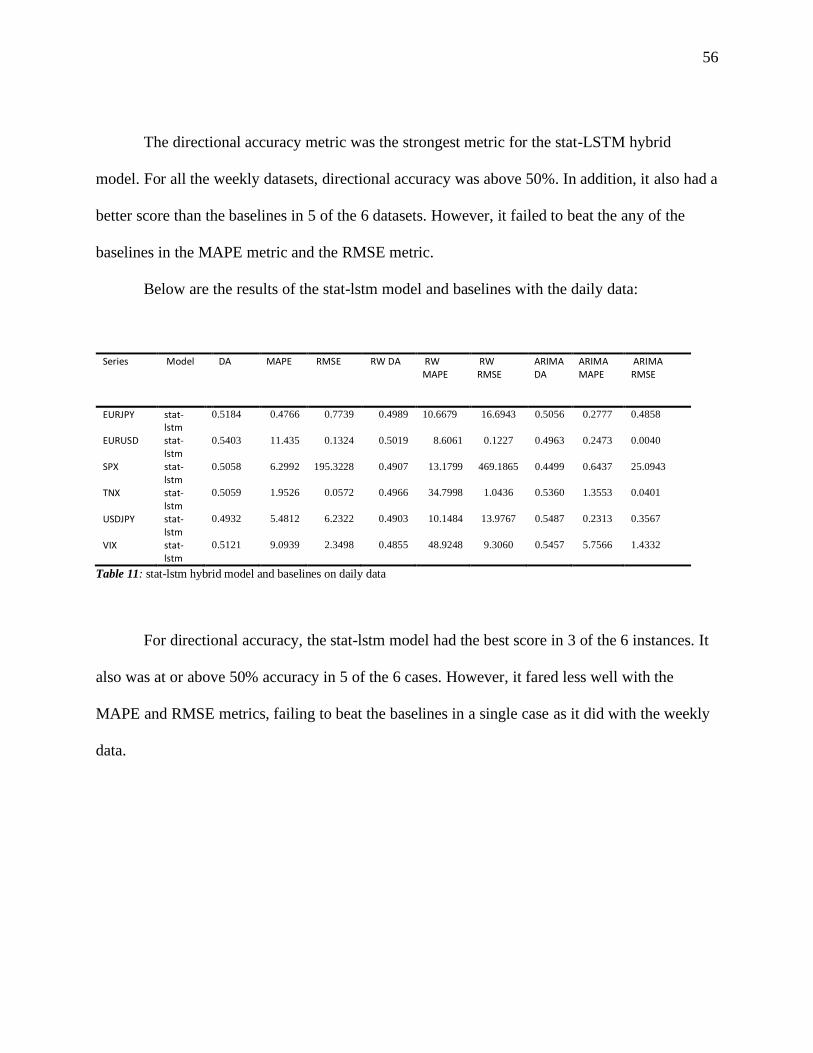
56

The directional accuracy metric was the strongest metric for the stat-LSTM hybrid

model. For all the weekly datasets, directional accuracy was above 50%. In addition, it also had a

better score than the baselines in 5 of the 6 datasets. However, it failed to beat the any of the

baselines in the MAPE metric and the RMSE metric.

Below are the results of the stat-lstm model and baselines with the daily data:

Series Model DA MAPE RMSE RW DA RW MAPE

RW RMSE

ARIMA DA

ARIMA MAPE

ARIMA RMSE

EURJPY stat-lstm

0.5184 0.4766 0.7739 0.4989 10.6679 16.6943 0.5056 0.2777 0.4858

EURUSD stat-lstm

0.5403 11.435 0.1324 0.5019 8.6061 0.1227 0.4963 0.2473 0.0040

SPX stat-lstm

0.5058 6.2992 195.3228 0.4907 13.1799 469.1865 0.4499 0.6437 25.0943

TNX stat-lstm

0.5059 1.9526 0.0572 0.4966 34.7998 1.0436 0.5360 1.3553 0.0401

USDJPY stat-lstm

0.4932 5.4812 6.2322 0.4903 10.1484 13.9767 0.5487 0.2313 0.3567

VIX stat-lstm

0.5121 9.0939 2.3498 0.4855 48.9248 9.3060 0.5457 5.7566 1.4332

Table 11: stat-lstm hybrid model and baselines on daily data

For directional accuracy, the stat-lstm model had the best score in 3 of the 6 instances. It

also was at or above 50% accuracy in 5 of the 6 cases. However, it fared less well with the

MAPE and RMSE metrics, failing to beat the baselines in a single case as it did with the weekly

data.

57

Figure 11: Stat-LSTM model on the TNX index

CNN-LSTM Hybrid Model Results

Drawing inspiration from the Wavenet model in Borovykh et al. (2017), this work used

dilated convolutional layers as a way to detect features in the time series data and merged that

with the LSTM model network. The results compared favorably to the other approaches. As with

the other approaches, the mean was taken of 10 runs on each dataset to calculate the metrics.

Below is a table that summarizes the CNN-LSTM hybrid model and the baselines on the weekly

data:

58

Series Model DA MAPE RMSE RW DA RW MAPE

RW RMSE

ARIMA DA

ARIMA MAPE

ARIMA RMSE

EURJPY cnn-lstm

0.5778 0.7172 1.1539 0.5000 10.7871 16.956 0.4556 0.7165 1.1515

EURUSD cnn-lstm

0.5589 0.6324 0.0086 0.4689 8.4865 0.1193 0.3444 0.6389 0.0086

SPX cnn-lstm

0.4622 2.884 94.016 0.4955 13.2815 474.934 0.4333 1.5107 55.2267

TNX cnn-lstm

0.5322 3.1802 0.0911 0.4822 35.1510 1.0494 0.5111 3.0998 0.0924

USDJPY cnn-lstm

0.5144 0.6643 0.8912 0.4756 10.2113 13.9049 0.5444 0.6572 0.8752

VIX cnn-lstm

0.6189 10.4431 2.5081 0.5022 50.8901 9.4771 0.5000 10.6352 2.5214

Table 12: cnn-lstm hybrid model and baselines on weekly data

The cnn-lstm hybrid model beat the baselines in the directional accuracy metric on the

weekly data in 4 out of the 6 cases. In addition, for 5 of 6 instances, the DA score was above

50%, and in 1 instance, it was above 60% accuracy. For the MAPE metric, the hybrid model beat

the baselines 2 of 6 times, and for RMSE, it beat the baselines 3 of 6 times.

The table below contrasts the CNN-LSTM model with the baselines on the daily data:

Series Model DA MAPE RMSE RW DA RW MAPE

RW RMSE

ARIMA DA

ARIMA MAPE

ARIMA RMSE

EURJPY cnn-lstm

0.5109 0.2936 0.5027 0.4989 10.6679 16.6943 0.5056 0.2777 0.4858

EURUSD cnn-lstm

0.4854 0.2607 0.0041 0.5019 8.6061 0.1227 0.4963 0.2473 0.0040

SPX cnn-lstm

0.4530 12.9119 387.1402 0.4907 13.1799 469.1865 0.4499 0.6437 25.0943

TNX cnn-lstm

0.5041 1.3914 0.0413 0.4966 34.7998 1.0436 0.5360 1.3553 0.0401

USDJPY cnn-lstm

0.5146 0.2522 0.3743 0.4903 10.1484 13.9767 0.5487 0.2313 0.3567

VIX cnn-lstm

0.5791 5.8795 1.4804 0.4855 48.9248 9.3060 0.5457 5.7566 1.4332

Table 13: cnn-lstm hybrid model and baselines on daily data

With the daily data, the cnn-lstm hybrid model did not fare as well. It was able to beat the

baseline models in only 2 of the 6 cases for directional accuracy. However, 4 of the 6 DA scores

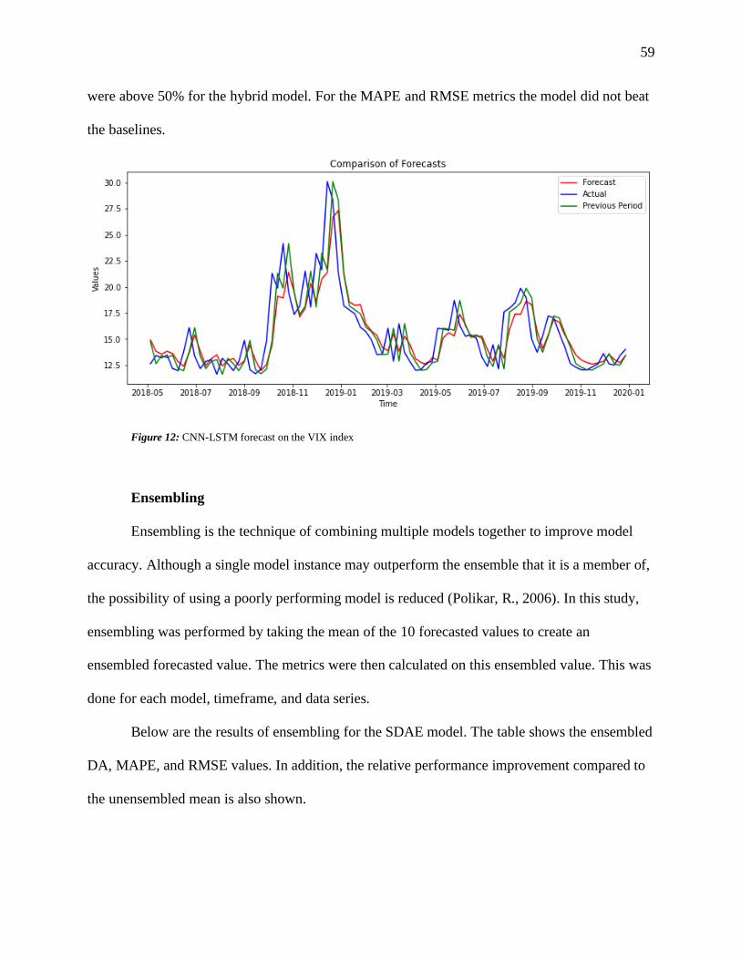
59

were above 50% for the hybrid model. For the MAPE and RMSE metrics the model did not beat

the baselines.

Figure 12: CNN-LSTM forecast on the VIX index

Ensembling

Ensembling is the technique of combining multiple models together to improve model

accuracy. Although a single model instance may outperform the ensemble that it is a member of,

the possibility of using a poorly performing model is reduced (Polikar, R., 2006). In this study,

ensembling was performed by taking the mean of the 10 forecasted values to create an

ensembled forecasted value. The metrics were then calculated on this ensembled value. This was

done for each model, timeframe, and data series.

Below are the results of ensembling for the SDAE model. The table shows the ensembled

DA, MAPE, and RMSE values. In addition, the relative performance improvement compared to

the unensembled mean is also shown.

60

Time frame

Series Model DA MAPE RMSE % DA Change

% MAPE Change

% RMSE Change

daily EURJPY sdae 0.5248 0.2803 0.4896 1.92 0.04 0.00

daily EURUSD sdae 0.4599 0.2487 0.0040 -1.56 0.04 0.00

daily SPX sdae 0.5604 0.6246 24.5362 0.00 0.02 0.01

daily TNX sdae 0.5300 1.3708 0.0403 1.15 0.00 0.00

daily USDJPY sdae 0.5095 0.2334 0.3597 1.13 0.04 0.00

daily VIX sdae 0.4419 5.7354 1.4164 -4.99 0.02 0.01

weekly EURJPY sdae 0.4000 0.7418 1.1809 -14.68 0.11 0.06

weekly EURUSD sdae 0.5250 0.6339 0.0084 -1.19 0.02 0.00

weekly SPX sdae 0.6125 1.4551 53.4207 0.41 0.00 0.01

weekly TNX sdae 0.6250 3.2247 0.0953 2.66 0.03 0.10

weekly USDJPY sdae 0.5125 0.6358 0.8547 -1.67 0.45 0.38

weekly VIX sdae 0.4375 10.2281 2.4005 -10.26 0.00 0.00

Table 14: SDAE Ensembled values and their relative improvement

Ensembling was of mixed benefit for the SDAE model, showing improvement across the

three metrics in some of the cases. For the DA metric ensembling improved 5 of the 12 series

instances. However, for 6 of the 12 instances, there was a net decrease in accuracy. For MAPE,

ensembling improved scores in 9 of the 12 instances. For the remainder of the instances there

was no change. Ensembling made a slight improvement with the RMSE score, making a small

improvement in 6 of the 12 instances.

Here are the results of ensembling for the LSTM model. As with the SDAE model, the

table shows the ensemble values for DA, MAPE, and RMSE, as well as their relative

improvement to the unensembled value:

61

Time frame

Series Model DA MAPE RMSE % DA Change

% MAPE Change

% RMSE Change

daily EURJPY lstm 0.5169 0.2826 0.4884 -0.71 0.81 0.47

daily EURUSD lstm 0.4813 0.2676 0.0041 -2.61 4.12 2.38

daily SPX lstm 0.5033 0.6954 26.3244 1.51 46.44 40.78

daily TNX lstm 0.4617 1.365 0.0402 -8.36 1.69 1.47

daily USDJPY lstm 0.5449 0.2347 0.3567 2.14 1.68 0.94

daily VIX lstm 0.6058 5.5739 1.4219 4.09 1.14 0.58

weekly EURJPY lstm 0.4444 0.7366 1.1635 -5.89 3.47 2.80

weekly EURUSD lstm 0.4778 1.2418 0.0161 -6.11 17.00 19.10

weekly SPX lstm 0.4000 8.188 241.4343 -15.29 14.77 15.96

weekly TNX lstm 0.5000 3.3148 0.0953 1.36 2.74 3.25

weekly USDJPY lstm 0.3889 0.6872 0.9146 -20.45 7.55 8.64

weekly VIX lstm 0.5778 10.2734 2.4950 -2.07 2.19 1.89

Table 15: LSTM Ensembled values and their relative improvement

For the LSTM model, ensembling improved the performance across the MAPE and

RMSE metrics. In two instances, the performance increase was by more than 40%. However, the

improvement for the DA metric was mixed with 4 of the 12 datasets showing an improvement

with this metric, but 8 of the datasets had a performance decrease.

The table below contains the results of ensembling for the CNN Wavenet inspired model:

62

Time frame

Series Model DA MAPE RMSE % DA Change

% MAPE Change

% RMSE Change

daily EURJPY cnn 0.4831 0.3507 0.5737 -3.67 32.93 29.66

daily EURUSD cnn 0.5206 0.2862 0.0043 0.29 41.14 37.68

daily SPX cnn 0.5212 1.2516 45.4498 1.22 15.74 13.14

daily TNX cnn 0.5135 1.5583 0.0462 -0.17 12.05 11.49

daily USDJPY cnn 0.5150 0.2585 0.3803 0.55 4.12 3.31

daily VIX cnn 0.5902 5.6560 1.4329 5.54 1.72 1.44

weekly EURJPY cnn 0.5444 0.9029 1.4075 -0.82 19.92 18.72

weekly EURUSD cnn 0.5556 0.6208 0.0083 2.68 4.09 6.74

weekly SPX cnn 0.5556 3.9058 139.7049 -1.96 3.81 2.14

weekly TNX cnn 0.4444 4.5946 0.1343 -4.08 10.79 10.88

weekly USDJPY cnn 0.5333 0.6550 0.8712 2.56 10.53 10.52

weekly VIX cnn 0.5889 10.2713 2.4592 -0.93 6.14 4.14

Table 16: cnn ensembled values and their relative improvement

Directional accuracy showed the least improvement among all of the metrics with 6 of

the 12 series showing an improvement, while the remaining showed a net performance decrease.

However, ensembling provided consistent performance improvements across all 12 datasets for

the CNN model with both the MAPE and RMSE metrics.

63

Below are the results of ensembling for the stat-LSTM hybrid:

Time frame

Series Model DA MAPE RMSE % DA Change

% MAPE Change

% RMSE Change

daily EURJPY stat-lstm 0.5357 0.4460 0.7310 3.34 6.42 5.54

daily EURUSD stat-lstm 0.5403 11.4350 0.1324 0.00 0.00 0.00

daily SPX stat-lstm 0.4720 3.2760 107.6501 -6.68 47.99 44.89

daily TNX stat-lstm 0.5057 1.9374 0.0567 -0.04 0.78 0.87

daily USDJPY stat-lstm 0.5133 4.5233 5.0583 4.08 17.48 18.84

daily VIX stat-lstm 0.5078 9.0227 2.3371 -0.84 0.78 0.54

weekly EURJPY stat-lstm 0.5238 1.2519 1.9161 -0.91 7.23 7.39

weekly EURUSD stat-lstm 0.5227 0.8211 0.0112 3.14 7.20 8.20

weekly SPX stat-lstm 0.5952 5.1104 170.5552 1.62 1.98 1.53

weekly TNX stat-lstm 0.5955 16.5567 0.4239 9.95 16.02 17.37

weekly USDJPY stat-lstm 0.5476 1.1827 1.6435 1.77 10.66 9.24

weekly VIX stat-lstm 0.5862 45.0459 7.9295 9.45 17.50 17.37

Table 17: stat-LSTM ensemble results and their relative improvement

The stat-LSTM hybrid model benefited from ensembling as with previous models. The

directional accuracy metric showed improved accuracy in 7 of the 12 time series instances. For

the MAPE and RMSE metrics, improvement was found by ensembling in 11 of the 12 series.

The CNN-LSTM hybrid model combines Wavenet inspired convolutions with an RNN

neural network. As with the other model variations, the CNN-LSTM showed metric performance

improvement from ensembling. The table below shows the summary results:

64

Time frame

Series Model DA MAPE RMSE % DA Change

% MAPE Change

% RMSE Change

daily EURJPY cnn-lstm 0.5112 0.2893 0.4969 0.06 1.46 1.15

daily EURUSD cnn -lstm 0.4775 0.2558 0.0040 -1.63 1.88 2.44

daily SPX cnn -lstm 0.4454 12.7428 382.3783 -1.68 1.31 1.23

daily TNX cnn -lstm 0.4910 1.3662 0.0407 -2.60 1.81 1.45

daily USDJPY cnn -lstm 0.5337 0.2407 0.3635 3.71 4.56 2.89

daily VIX cnn -lstm 0.5924 5.7704 1.4633 2.30 1.86 1.16

weekly EURJPY cnn -lstm 0.5889 0.6987 1.1300 1.92 2.58 2.07

weekly EURUSD cnn -lstm 0.6000 0.6309 0.0085 7.35 0.24 1.16

weekly SPX cnn -lstm 0.4444 2.8490 92.9795 -3.85 1.21 1.10

weekly TNX cnn -lstm 0.5333 3.1592 0.0906 0.21 0.66 0.55

weekly USDJPY cnn -lstm 0.5444 0.6542 0.8788 5.83 1.52 1.39

weekly VIX cnn -lstm 0.6000 10.3181 2.4539 -3.05 1.20 2.16

Table 18: cnn-lstm ensemble results and their relative improvement

Ensembling improved directional accuracy in 7 of the 12 cases. Ensembling consistently

improved the MAPE and RMSE metrics, showing a modest benefit in all of the cases.

Directional Accuracy

The directional accuracy metric can be further analyzed if it is thought of as a

classification problem. One class is defined as up, and the other is defined as down. This further

decomposition of directional accuracy can provide additional insight into the predictive power of

a model. One way to model this classification problem would be to treat up as a positive case and

down as the negative case and compute metrics such as precision and recall based on this

assumption. However, it is possible that some models are unusually good at predicting only one

65

direction. Because of this, it can be useful to think of up and down as separate classification

problems and compute the metrics precision, recall, and F1 for both.

With directional accuracy seen as a classification problem, it can also be informative to

compare the models against a new baseline for classification: always predicting one class. For

instance, the new baseline ‘always up’ would predict up every time. This research includes the

precision and recall scores for always up and always down. The results presented in the

following tables include the mean of 10 runs for each model.

The table below lists the precision and recall scores for each model and the EURJPY

series. There are two precision scores for each model: the precision score for predicting the down

direction, and a separate score for predicting the up direction; similarly, there are two recall

scores for each model. The F1 score is a harmonic of the precision and recall scores; an F1 value

for the up and down categories is also provided.

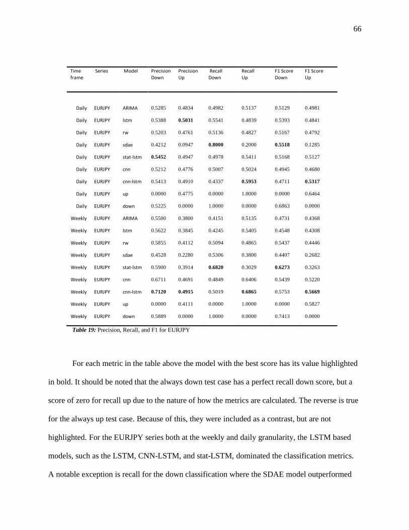
66

Time frame

Series Model Precision Down

Precision Up

Recall Down

Recall Up

F1 Score Down

F1 Score Up

Daily EURJPY ARIMA 0.5285 0.4834 0.4982 0.5137 0.5129 0.4981

Daily EURJPY lstm 0.5388 0.5031 0.5541 0.4839 0.5393 0.4841

Daily EURJPY rw 0.5203 0.4761 0.5136 0.4827 0.5167 0.4792

Daily EURJPY sdae 0.4212 0.0947 0.8000 0.2000 0.5518 0.1285

Daily EURJPY stat-lstm 0.5452 0.4947 0.4978 0.5411 0.5168 0.5127

Daily EURJPY cnn 0.5212 0.4776 0.5007 0.5024 0.4945 0.4680

Daily EURJPY cnn-lstm 0.5413 0.4910 0.4337 0.5953 0.4711 0.5317

Daily EURJPY up 0.0000 0.4775 0.0000 1.0000 0.0000 0.6464

Daily EURJPY down 0.5225 0.0000 1.0000 0.0000 0.6863 0.0000

Weekly EURJPY ARIMA 0.5500 0.3800 0.4151 0.5135 0.4731 0.4368

Weekly EURJPY lstm 0.5622 0.3845 0.4245 0.5405 0.4548 0.4308

Weekly EURJPY rw 0.5855 0.4112 0.5094 0.4865 0.5437 0.4446

Weekly EURJPY sdae 0.4528 0.2280 0.5306 0.3800 0.4407 0.2682

Weekly EURJPY stat-lstm 0.5900 0.3914 0.6820 0.3029 0.6273 0.3263

Weekly EURJPY cnn 0.6711 0.4691 0.4849 0.6406 0.5439 0.5220

Weekly EURJPY cnn-lstm 0.7120 0.4915 0.5019 0.6865 0.5753 0.5669

Weekly EURJPY up 0.0000 0.4111 0.0000 1.0000 0.0000 0.5827

Weekly EURJPY down 0.5889 0.0000 1.0000 0.0000 0.7413 0.0000

Table 19: Precision, Recall, and F1 for EURJPY

For each metric in the table above the model with the best score has its value highlighted

in bold. It should be noted that the always down test case has a perfect recall down score, but a

score of zero for recall up due to the nature of how the metrics are calculated. The reverse is true

for the always up test case. Because of this, they were included as a contrast, but are not

highlighted. For the EURJPY series both at the weekly and daily granularity, the LSTM based

models, such as the LSTM, CNN-LSTM, and stat-LSTM, dominated the classification metrics.

A notable exception is recall for the down classification where the SDAE model outperformed

67

the others at the daily granularity on recall down and the F1 down scores. However, this good

performance with recall for down classifications was matched with correspondingly poor scores

for the up metrics.

The table below shows the results of directional accuracy as a classification metric for the

EURUSD dataset:

Time frame

Series Model Precision Down

Precision Up

Recall Down

Recall Up

F1 Score Down

F1 Score Up

Daily EURUSD ARIMA 0.5355 0.4524 0.5225 0.4653 0.5289 0.4588

Daily EURUSD lstm 0.5299 0.4445 0.5716 0.4028 0.5255 0.3867

Daily EURUSD rw 0.5441 0.4616 0.4907 0.5151 0.5158 0.4867

Daily EURUSD sdae 0.0823 0.4641 0.0828 0.9185 0.0679 0.5966

Daily EURUSD stat-lstm 0.5403 0.0000 1.0000 0.0000 0.7016 0.0000

Daily EURUSD cnn 0.5440 0.4550 0.7263 0.2747 0.6083 0.2984

Daily EURUSD cnn-lstm 0.5310 0.4513 0.4000 0.5861 0.4323 0.4975

Daily EURUSD up 0.0000 0.4588 0.0000 1.0000 0.0000 0.6290

Daily EURUSD down 0.5412 0.0000 1.0000 0.0000 0.7023 0.0000

Weekly EURUSD ARIMA 0.4151 0.2432 0.4400 0.2250 0.4272 0.2338

Weekly EURUSD lstm 0.6744 0.4836 0.3080 0.7600 0.3284 0.5482

Weekly EURUSD rw 0.5277 0.4173 0.4420 0.5025 0.4799 0.4552

Weekly EURUSD sdae 0.5352 0.0908 0.9477 0.0700 0.6754 0.0667

Weekly EURUSD stat-lstm 0.5505 0.3788 0.6327 0.3487 0.5769 0.3496

Weekly EURUSD cnn 0.5496 0.4672 0.6660 0.3850 0.5720 0.3501

Weekly EURUSD cnn-lstm 0.5906 0.5109 0.6820 0.4050 0.6182 0.4148

Weekly EURUSD up 0.0000 0.4444 0.0000 1.0000 0.0000 0.6154

Weekly EURUSD down 0.5556 0.0000 1.0000 0.0000 0.7143 0.0000

Table 20: Precision, Recall, and F1 for EURUSD

For the EURUSD datasets, the best scores were distributed between RNN based models

and the SDAE. The ARIMA and random walk baselines were beaten in nearly every case, with

68

one exception: the random walk model at the daily granularity edged out the CNN model for the

precision down score top spot. Another interesting case was the stat-LSTM hybrid at the daily

granularity. It had a perfect score recall down, and a score of zero for precision up, mimicking

the behavior of always predicting the next value as down.

Below is the table listing the directional accuracy classification results for the USDJPY

series:

Time frame

Series Model Precision Down

Precision Up

Recall Down

Recall Up

F1 Score Down

F1 Score Up

Daily USDJPY ARIMA 0.5328 0.5654 0.5637 0.5345 0.5478 0.5495

Daily USDJPY lstm 0.5321 0.5525 0.5328 0.5342 0.5046 0.5062

Daily USDJPY rw 0.4756 0.5048 0.4880 0.4924 0.4817 0.4984

Daily USDJPY sdae 0.1472 0.3567 0.3000 0.7000 0.1975 0.4725

Daily USDJPY stat-lstm 0.4291 0.5040 0.4712 0.5140 0.4318 0.4777

Daily USDJPY cnn 0.5011 0.5302 0.5904 0.4385 0.5313 0.4651

Daily USDJPY cnn-lstm 0.5050 0.5400 0.6236 0.4120 0.5415 0.4329

Daily USDJPY up 0.0000 0.515 0.0000 1.0000 0.0000 0.6799

Daily USDJPY down 0.4850 0.0000 1.0000 0.0000 0.6532 0.0000

Weekly USDJPY ARIMA 0.5000 0.5870 0.5366 0.5510 0.5176 0.5684

Weekly USDJPY lstm 0.4207 0.5465 0.4756 0.5000 0.3991 0.4659

Weekly USDJPY rw 0.4325 0.5189 0.4805 0.4714 0.4535 0.4919

Weekly USDJPY sdae 0.5067 0.2313 0.7900 0.2591 0.5886 0.2426

Weekly USDJPY stat-lstm 0.5123 0.6157 0.7200 0.3727 0.5932 0.4435

Weekly USDJPY cnn 0.4753 0.5948 0.5902 0.4612 0.4971 0.4789

Weekly USDJPY cnn-lstm 0.4666 0.5499 0.4439 0.5735 0.4246 0.5396

Weekly USDJPY up 0.0000 0.5444 0.0000 1.0000 0.0000 0.7050

Weekly USDJPY down 0.4556 0.0000 1.0000 0.0000 0.6260 0.0000

Table 21: Precision, Recall, and F1 on USDJPY

69

For the USDJPY series, the baselines fared a little better than in the previous two

instances. The ARIMA model dominated the scores at the daily granularity, having the best score

in 4 of the 6 categories, with the SDAE and CNN-LSTM each showing the best in a single

category. At the weekly level, the RNN based models had the strongest results, with the CNN-

LSTM having the best results in a single instance, and the stat-LSTM hybrid having 3 of the 6

strongest scores. The SDAE and ARIMA models each had the best score in a single category.

The table below details the precision, recall, and F1 scores for the SPX index:

Time frame

Series Model Precision Down

Precision Up

Recall Down

Recall Up

F1 Score Down

F1 Score Up

Daily SPX ARIMA 0.4152 0.5058 0.5750 0.3494 0.4822 0.4133

Daily SPX lstm 0.4195 0.5985 0.4670 0.5189 0.3556 0.4154

Daily SPX rw 0.4349 0.5444 0.4790 0.5000 0.4558 0.5211

Daily SPX sdae 0.0000 0.5621 0.0000 1.0000 0.0000 0.7197

Daily SPX stat-lstm 0.3868 0.3330 0.4477 0.5524 0.3187 0.4149

Daily SPX cnn 0.4059 0.5472 0.2450 0.7317 0.2683 0.6094

Daily SPX cnn-lstm 0.4476 0.3326 0.9670 0.0402 0.6110 0.0621

Daily SPX up 0.0000 0.5621 0.0000 1.0000 0.0000 0.7197

Daily SPX down 0.4454 0.0000 1.0000 0.0000 0.6163 0.0000

Weekly SPX ARIMA 0.3529 0.5385 0.5000 0.3889 0.4138 0.4516

Weekly SPX lstm 0.3997 0.5827 0.6833 0.3315 0.4919 0.3906

Weekly SPX rw 0.3971 0.5985 0.5083 0.4870 0.4451 0.5361

Weekly SPX sdae 0.0933 0.6198 0.0188 0.9846 0.0309 0.7605

Weekly SPX stat-lstm 0.4972 0.6010 0.0364 0.9412 0.0637 0.7332

Weekly SPX cnn 0.3223 0.5930 0.0972 0.8796 0.1307 0.7052

Weekly SPX cnn-lstm 0.4179 0.7030 0.8778 0.1852 0.5659 0.2895

Weekly SPX up 0.0000 0.6000 0.0000 1.0000 0.0000 0.7500

Weekly SPX down 0.4000 0.0000 1.0000 0.0000 0.5714 0.0000

Table 22: Precision, Recall, and F1 for the SPX

70

For the SPX, the RNN based models had a strong showing, with the CNN-LSTM having

the best score in 3 of the 6 metrics at the daily level. The LSTM scored the best at the daily

granularity in a single category. The SDAE had two of the best metrics scores at the daily level,

but the scores indicate the SDAE predictions were little better than always predicting up as a

directional forecast.

For the weekly granularity, the RNN based models again had a strong showing: the

CNN-LSTM had the best scores in 3 of the best categories, and the stat-LSTM had the best score

in a single category. The SDAE had the best score in two categories.

Below are the classification metrics for the interest rate index, the TNX:

71

Time frame

Series Model Precision Down

Precision Up

Recall Down

Recall Up

F1 Score Down

F1 Score Up

Daily TNX ARIMA 0.5736 0.5061 0.4809 0.5981 0.5231 0.5482

Daily TNX lstm 0.5529 0.4820 0.4613 0.5517 0.4333 0.4669

Daily TNX rw 0.5255 0.4679 0.4949 0.4986 0.5097 0.4827

Daily TNX sdae 0.4767 0.0470 0.9000 0.1000 0.6233 0.0640

Daily TNX stat-lstm 0.5336 0.4801 0.4884 0.5254 0.5083 0.5001

Daily TNX cnn 0.5395 0.4837 0.5847 0.4354 0.5485 0.4428

Daily TNX cnn-lstm 0.5450 0.4791 0.4362 0.5804 0.4548 0.4988

Daily TNX up 0.0000 0.4707 0.0000 1.0000 0.0000 0.6401

Daily TNX down 0.5293 0.0000 1.0000 0.0000 0.6922 0.0000

Weekly TNX ARIMA 0.6136 0.4130 0.5000 0.5278 0.5510 0.4634

Weekly TNX lstm 0.6176 0.3946 0.4630 0.5389 0.4983 0.4352

Weekly TNX rw 0.5832 0.3789 0.4889 0.4722 0.5311 0.4198

Weekly TNX sdae 0.6687 0.3343 0.7962 0.3064 0.7166 0.3099

Weekly TNX stat-lstm 0.6065 0.2940 0.6698 0.3528 0.6202 0.3202

Weekly TNX cnn 0.7060 0.4097 0.2518 0.7805 0.3241 0.5304

Weekly TNX cnn-lstm 0.6140 0.4157 0.6000 0.4306 0.6045 0.4197

Weekly TNX up 0.0000 0.4000 0.0000 1.0000 0.0000 0.5714

Weekly TNX down 0.6000 0.0000 1.0000 0.0000 0.7500 0.000

Table 23: Precision, Recall, and F1 for the TNX

The ARIMA model did the best on the TNX index at the daily granularity, having 4 of

the 6 possible highest classification metric scores. At the daily level, the SDAE had the other 2

top scores. For the weekly level of granularity, CNN based models did the best with the Wavenet

based CNN model having 3 of the 6 best scores, and the CNN-LSTM in a single instance. The

SDAE had 2 of the 6 best scores. LSTM models were not good candidates for classification on

the TNX dataset, with only the CNN-LSTM variant doing the best in 1 category.

72

Below is the table summarizing the classification performance on the VIX at the daily

and weekly granularity:

Time frame

Series Model Precision Down

Precision Up

Recall Down

Recall Up

F1 Score Down

F1 Score Up

Daily VIX ARIMA 0.6307 0.4908 0.4440 0.6734 0.5211 0.5678

Daily VIX lstm 0.6235 0.5552 0.6724 0.4683 0.6225 0.4745

Daily VIX rw 0.5426 0.4288 0.4856 0.4854 0.5123 0.4551

Daily VIX sdae 0.1115 0.3539 0.2000 0.8000 0.1432 0.4908

Daily VIX stat-lstm 0.5603 0.4556 0.5470 0.4690 0.5520 0.4605

Daily VIX cnn 0.5902 0.5046 0.7020 0.3799 0.6360 0.4182

Daily VIX cnn-lstm 0.6336 0.5280 0.5940 0.5603 0.6053 0.5334

Daily VIX up 0.0000 0.4432 0.0000 1.0000 0.0000 0.6142

Daily VIX down 0.5568 0.0000 1.0000 0.0000 0.7153 0.0000

Weekly VIX ARIMA 0.5946 0.4340 0.4231 0.6053 0.4944 0.5055

Weekly VIX lstm 0.6625 0.5243 0.5884 0.5921 0.6189 0.5487

Weekly VIX rw 0.5809 0.4212 0.5077 0.4947 0.5401 0.4534

Weekly VIX sdae 0.2238 0.2643 0.4000 0.6000 0.2870 0.3670

Weekly VIX stat-lstm 0.5703 0.1492 0.7863 0.1806 0.6445 0.1633

Weekly VIX cnn 0.6881 0.5290 0.5615 0.6395 0.6036 0.5639

Weekly VIX cnn-lstm 0.7018 0.5429 0.5923 0.6553 0.6402 0.5920

Weekly VIX up 0.0000 0.4222 0.0000 1.0000 0.0000 0.5938

Weekly VIX down 0.5778 0.0000 1.0000 0.0000 0.7324 0.0000

Table 24: Precision, Recall, and F1 scores for the VIX

For the VIX at the daily level of granularity, there was no clear best model. The CNN

model scored the best in 2 of the 6 categories, and the ARIMA, LSTM, CNN-LSTM, and SDAE

models all having the best score in a single category. For the weekly level, the RNN based

models dominated the metrics with the CNN-LSTM having the best score in 4 of 6 categories,

and the stat-LSTM model having the best score in 2 of the 6 categories.

73

Directional Accuracy Summary

Decomposition of the directional accuracy score into precision, recall, and F1 for both the

up case and the down case provide additional insight into the predictive power of the models for

direction. When viewing the data at both the daily and weekly granularity, the CNN-LSTM

hybrid model scores the best in the greatest number of categories. Much of its strength comes

from its predictive power at the weekly level. If the daily granularity is only considered, the

SDAE has the best predictive power. However, if the LSTM and associated hybrid models, stat-

LSTM and CNN-LSTM are considered at the daily level, as a group they score better in a greater

number of categories than the SDAE model. If the category of up is only considered, the CNN-

LSTM hybrid model is the best predictor. However, the best predictor for the category down is

examined, the stat-LSTM model is the best predictor.

k-ahead Predictions

Forecasting problems can require a forecast or prediction not just for the next time

period, but for multiple time periods ahead. Forecasting requirements can include forecasting not

only for 𝑦𝑡+1, but for 𝑦𝑡+2,…, 𝑦𝑡+𝑘 , This research includes a comparison of the models and

baselines on multi-step ahead predictions using the metrics defined previously: DA, MAPE, and

RMSE. The data used in this evaluation consisted of the ensembled model runs. The t+k head

predictions will be done in a recursive fashion:

Prediction(t+1) takes as input data(t), data(t-1), data(t-2)…

Prediction(t+2) takes as input prediction(t+1), data(t), data(t-1),…

Prediction(t+3) takes as input prediction(t+2), prediction(t+1), data(t),…

The figure below illustrates how this will work:

74

Figure 13: t+k ahead predictions

The value for k in this study is 3. For each value of k, the DA, MAPE, and RMSE will be

calculated, and the models will be compared by dataset series and timeframe. The best value for

each metric will be highlighted in bold. The table below shows the results of the t+k ahead

predictions for the EURJPY series at the weekly and monthly granularity:

Time frame

Model DA (t+1)

DA (t+2)

DA (t+3)

MAPE (t+1)

MAPE (t+2)

MAPE (t+3)

RMSE (t+1)

RMSE (t+2)

RMSE (t+3)

daily ARIMA 0.5056 0.5169 0.4888 0.2777 0.4166 0.5268 0.4858 0.6847 0.8456

daily lstm 0.5169 0.4813 0.4831 0.2826 0.4237 0.5338 0.4884 0.6900 0.8498

daily rw 0.5 0.5112 0.4869 3.5024 4.9263 6.1793 5.3802 7.644 9.3594

daily sdae 0.5248 0.5267 0.5286 0.2803 0.2798 0.2800 0.4896 0.4892 0.4894

daily stat-lstm 0.5357 0.4925 0.4699 0.4460 0.6515 0.7957 0.7310 1.0411 1.2844

daily cnn 0.4831 0.4906 0.5112 0.3507 0.4676 0.5664 0.5737 0.7584 0.9154

daily cnn-lstm 0.5112 0.4981 0.4963 0.2893 0.4241 0.5328 0.4969 0.6977 0.8526

weekly ARIMA 0.4556 0.4667 0.5111 0.7165 1.0450 1.2171 1.1515 1.5685 1.8610

weekly lstm 0.4444 0.4889 0.5222 0.7366 1.0180 1.1927 1.1635 1.5650 1.8480

weekly rw 0.4778 0.4889 0.4222 3.5064 4.9122 6.1741 5.6668 7.5509 9.3987

weekly sdae 0.4000 0.4625 0.4750 0.7418 0.7279 0.7279 1.1809 1.1464 1.1459

weekly stat-lstm 0.5238 0.5833 0.4643 1.2519 1.7551 2.1712 1.9161 2.7178 3.3071

weekly cnn 0.5444 0.5556 0.5444 0.9029 1.0917 1.2613 1.4075 1.6867 1.9408

weekly cnn-lstm 0.5889 0.5667 0.5222 0.6987 0.9551 1.1371 1.1300 1.4734 1.7268

Table 25: t+k ahead prediction metrics for EURJPY

75

For the directional accuracy metric at the daily granularity, the stat-LSTM hybrid had the

best score at t+1, but the accuracy dropped off quickly at subsequent steps. At both the daily and

weekly granularity, the SDAE proved to be an effective model, having the strongest scores in

the MAPE and RMSE metrics at the t+2 and t+3. For directional accuracy at the weekly

granularity, the CNN-LSTM hybrid, the CNN, and the stat-LSTM hybrid model each had a best

score.

The table below shows the t+k ahead predictions for the EURUSD time series:

Time frame

Model DA (t+1)

DA (t+2)

DA (t+3)

MAPE (t+1)

MAPE (t+2)

MAPE (t+3)

RMSE (t+1)

RMSE (t+2)

RMSE (t+3)

daily ARIMA 0.4963 0.5337 0.5075 0.2473 0.3680 0.4504 0.0040 0.0054 0.0064

daily lstm 0.4813 0.5225 0.4738 0.2676 0.3997 0.4956 0.0041 0.0058 0.0070

daily rw 0.5056 0.4494 0.4888 2.5673 3.8424 4.8710 0.0371 0.0547 0.0698

daily sdae 0.4599 0.458 0.4599 0.2487 0.2476 0.2476 0.0040 0.0040 0.0040

daily stat-lstm 0.5403 0.5422 0.5403 11.435 11.4523 11.4699 0.1324 0.1325 0.1327

daily cnn 0.5206 0.5075 0.5112 0.2862 0.4135 0.5265 0.0043 0.006 0.0076

daily cnn-lstm 0.4775 0.5187 0.4888 0.2558 0.3742 0.4534 0.0040 0.0055 0.0065

weekly ARIMA 0.3444 0.5889 0.6222 0.6389 0.7547 0.8011 0.0086 0.0110 0.0126

weekly lstm 0.4778 0.5111 0.4889 1.2418 1.5360 1.7807 0.0161 0.0194 0.0224

weekly rw 0.4333 0.5000 0.5000 2.7440 3.7743 4.7630 0.0384 0.0516 0.0663

weekly sdae 0.5250 0.5250 0.5375 0.6339 0.6280 0.6305 0.0084 0.0083 0.0083

weekly stat-lstm 0.5227 0.5227 0.5114 0.8211 1.0667 1.3245 0.0112 0.0147 0.0190

weekly cnn 0.5556 0.6333 0.6222 0.6208 0.6934 0.7760 0.0083 0.0104 0.0120

weekly cnn-lstm 0.6000 0.6222 0.6222 0.6309 0.7335 0.8065 0.0085 0.0110 0.0129

Table 26: t+k ahead predictions for EURUSD

At the daily granularity, the stat-LSTM hybrid model consistently had the best scores for

directional accuracy, an interesting contrast to its behavior on the EURJPY model, where the

predictive accuracy dropped off with subsequent timesteps. For MAPE, the ARIMA model had

the best score at t+1, and the SDAE again had good scores at t+2 and t+3. For the RMSE score,

at t+1, there was a three-way tie between the ARIMA, SDAE, and CNN-LSTM hybrid models.

However, the scores for the ARIMA and CNN-LSTM models gradually got worse, but the

SDAE model continued to have a strong score at t+2 and t+3.

76

At the weekly level of granularity, the CNN based models had the best directional

accuracy scores, with the CNN-LSTM hybrid having the best score at t+1, the CNN having the

best score at t+2, and at t+3, there was a three-way tie between the CNN, CNN-LSTM, and the

ARIMA models. For the MAPE and RMSE scores, the CNN model had the best prediction at

t+1, but the SDAE again showed strength at t+2 and t+3, having the best score for both metrics

at those steps.

The table below shows the t+k ahead predictions on the USDJPY series:

Time frame

Model DA (t+1)

DA (t+2)

DA (t+3)

MAPE (t+1)

MAPE (t+2)

MAPE (t+3)

RMSE (t+1)

RMSE (t+2)

RMSE (t+3)

daily ARIMA 0.5487 0.5262 0.4963 0.2313 0.3337 0.4282 0.3567 0.4828 0.6016

daily lstm 0.5449 0.5318 0.4981 0.2347 0.3365 0.4298 0.3567 0.4837 0.6027

daily rw 0.4644 0.5019 0.5056 3.3402 4.6142 5.3581 4.6233 6.3269 7.4445

daily sdae 0.5095 0.5095 0.5076 0.2334 0.2316 0.2327 0.3597 0.3566 0.3577

daily stat-lstm 0.5133 0.5133 0.5114 4.5233 4.5293 4.5283 5.0583 5.0881 5.1030

daily cnn 0.5150 0.5075 0.5131 0.2585 0.3611 0.4558 0.3803 0.5120 0.6319

daily cnn-lstm 0.5337 0.5112 0.4869 0.2407 0.3431 0.4347 0.3635 0.4926 0.6081

weekly ARIMA 0.5444 0.5889 0.5667 0.6572 0.8200 0.9838 0.8752 1.1203 1.3628

weekly lstm 0.3889 0.5889 0.6222 0.6872 0.8397 0.9734 0.9146 1.1728 1.3794

weekly rw 0.4333 0.4667 0.5556 3.0324 4.3117 5.2652 4.0887 5.8496 7.1095

weekly sdae 0.5125 0.4625 0.4625 0.6358 0.6310 0.6302 0.8547 0.8476 0.8482

weekly stat-lstm 0.5476 0.5595 0.5476 1.1827 1.7424 2.3308 1.6435 2.3737 3.1400

weekly cnn 0.5333 0.6000 0.5778 0.6550 0.8097 0.9855 0.8712 1.1218 1.3518

weekly cnn-lstm 0.5444 0.6000 0.6111 0.6542 0.8151 0.9582 0.8788 1.1321 1.3352

Table 27: t+k ahead predictions for USDJPY

At the daily granularity, the ARIMA model had the best score for DA, MAPE, and

RMSE at the t+1 step. At the t+2 step, the LSTM model had the best DA score, while the CNN

model had the best score at the t+3 step. For MAPE and RMSE, the SDAE model again showed

solid performance, having the best scores at the t+2 and t+3 steps, both at the daily and weekly

level of granularity. At the weekly level, directional accuracy the stat-LSTM had the best score

at the t+1 step, the CNN and CNN-LSTM models tied for the best score at the t+2 step, and the

LSTM had the best score at the t+3 step.

77

The table below contains the results for the SPX datasets at the daily and weekly

granularity:

Time frame

Model DA (t+1)

DA (t+2)

DA (t+3)

MAPE (t+1)

MAPE (t+2)

MAPE (t+3)

RMSE (t+1)

RMSE (t+2)

RMSE (t+3)

daily ARIMA 0.4499 0.4811 0.4722 0.6437 0.9389 1.1448 25.0943 34.7663 42.1024

daily lstm 0.5033 0.5234 0.5234 0.6954 1.0209 1.3097 26.3244 37.3716 47.3455

daily rw 0.4499 0.5033 0.5167 4.1989 5.9069 7.1769 143.7868 207.2171 245.0105

daily sdae 0.5604 0.5604 0.5626 0.6246 0.6249 0.6220 24.5362 24.5443 24.4873

daily stat-lstm 0.4720 0.4877 0.4966 3.2760 2.9680 2.9955 107.6501 102.3991 105.2444

daily cnn 0.5212 0.5212 0.5278 1.2516 1.3800 1.7372 45.4498 49.9295 62.3411

daily cnn-lstm 0.4454 0.4432 0.4432 12.7428 12.7567 12.8036 382.3783 383.1519 384.8634

weekly ARIMA 0.4333 0.4556 0.4000 1.5107 2.0837 2.6471 55.2267 73.4156 92.1557

weekly lstm 0.4000 0.4000 0.3889 8.188 8.8999 9.5858 241.4343 267.9237 290.1576

weekly rw 0.4667 0.4889 0.4889 4.4482 6.1140 8.1853 156.6434 218.4162 283.9419

weekly sdae 0.6125 0.6125 0.6125 1.4551 1.4602 1.4739 53.4207 53.4826 53.7626

weekly stat-lstm 0.5952 0.6190 0.6310 5.1104 7.2788 8.9327 170.5552 238.0102 289.0668

weekly cnn 0.5556 0.5667 0.5778 3.9058 4.2305 4.7880 139.7049 151.0134 169.7994

weekly cnn-lstm 0.4444 0.4333 0.4444 2.8490 3.4824 4.2082 92.9795 112.6851 137.1285

Table 28: t+k ahead predictions for the SPX

At the daily granularity, the SDAE model had the best metrics scores across time periods:

t+1, t+2, and t+3, as well as across all three metrics: DA, MAPE, and RMSE. At the weekly

granularity, the SDAE had the best DA score at t+1, but at t+2 and t+3, was beaten by the stat-

LSTM hybrid model. For the MAPE, and RMSE metrics, the SDAE again had the best metrics

across all three time steps.

Below is the table containing the t+k ahead predictions for the TNX index:

78

Time frame

Model DA (t+1)

DA (t+2)

DA (t+3)

MAPE (t+1)

MAPE (t+2)

MAPE (t+3)

RMSE (t+1)

RMSE (t+2)

RMSE (t+3)

daily ARIMA 0.5360 0.5383 0.5203 1.3553 1.8697 2.2844 0.0401 0.0547 0.0696

daily lstm 0.4617 0.5563 0.5338 1.3650 1.8598 2.2913 0.0402 0.0545 0.0692

daily rw 0.4752 0.5315 0.5000 10.9339 15.6357 18.7962 0.3311 0.4665 0.5533

daily sdae 0.5300 0.5300 0.5300 1.3708 1.3697 1.3726 0.0403 0.0402 0.0402

daily stat-lstm 0.5057 0.5329 0.5057 1.9374 2.5593 3.1581 0.0567 0.0758 0.0944

daily cnn 0.5135 0.5113 0.4955 1.5583 2.0419 2.5624 0.0462 0.0606 0.0758

daily cnn-lstm 0.4910 0.5203 0.5180 1.3662 1.9059 2.3469 0.0407 0.0557 0.0703

weekly ARIMA 0.5111 0.5000 0.4889 3.0998 4.5629 5.6353 0.0924 0.1292 0.1623

weekly lstm 0.5000 0.5111 0.5111 3.3148 4.6855 5.6220 0.0953 0.1292 0.1594

weekly rw 0.5111 0.4556 0.5556 12.4681 16.5009 20.6381 0.3805 0.4774 0.6408

weekly sdae 0.6250 0.6125 0.6375 3.2247 3.1765 3.2286 0.0953 0.0942 0.0950

weekly stat-lstm 0.5955 0.5955 0.5955 16.5567 16.4966 16.5467 0.4239 0.4236 0.4290

weekly cnn 0.4444 0.4667 0.4667 4.5946 6.9301 9.9019 0.1343 0.2105 0.3146

weekly cnn-lstm 0.5333 0.5889 0.5222 3.1592 4.3909 5.2765 0.0906 0.1227 0.1527

Table 29: t+k ahead predictions for the TNX

At the daily level of granularity, the ARIMA metric had the best directional accuracy

score at the t+1 time step and the LSTM had the best directional accuracy score at both the t+2

and t+3 timesteps. The ARIMA model also had the best score at the t+1 time step for the MAPE

and RMSE metrics, while the SDAE model had the best accuracy at the t+2 and t+3 timesteps.

At the weekly level of granularity, the SDAE had the best directional accuracy score at

the t+1, t+2, and t+3 time steps. The ARIMA model had the best accuracy at the t+1 time step

for the MAPE. The CNN-LSTM model had the best accuracy at the t+1 time step for the RMSE.

The SDAE had the best accuracy at the t+2 and t+3 timesteps for both the MAPE and RMSE

scores.

The table below shows the t+k ahead predictions for the VIX:

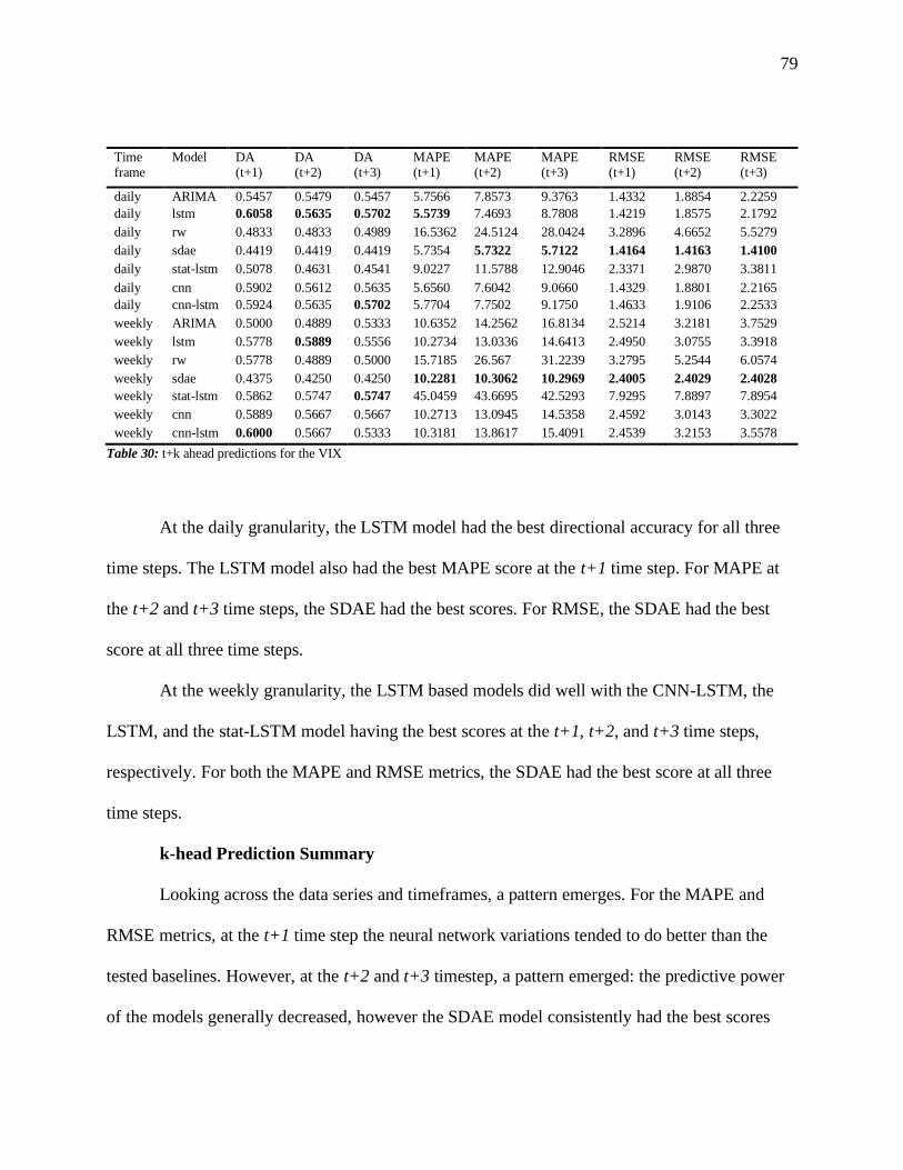
79

Time frame

Model DA (t+1)

DA (t+2)

DA (t+3)

MAPE (t+1)

MAPE (t+2)

MAPE (t+3)

RMSE (t+1)

RMSE (t+2)

RMSE (t+3)

daily ARIMA 0.5457 0.5479 0.5457 5.7566 7.8573 9.3763 1.4332 1.8854 2.2259

daily lstm 0.6058 0.5635 0.5702 5.5739 7.4693 8.7808 1.4219 1.8575 2.1792

daily rw 0.4833 0.4833 0.4989 16.5362 24.5124 28.0424 3.2896 4.6652 5.5279

daily sdae 0.4419 0.4419 0.4419 5.7354 5.7322 5.7122 1.4164 1.4163 1.4100

daily stat-lstm 0.5078 0.4631 0.4541 9.0227 11.5788 12.9046 2.3371 2.9870 3.3811

daily cnn 0.5902 0.5612 0.5635 5.6560 7.6042 9.0660 1.4329 1.8801 2.2165

daily cnn-lstm 0.5924 0.5635 0.5702 5.7704 7.7502 9.1750 1.4633 1.9106 2.2533

weekly ARIMA 0.5000 0.4889 0.5333 10.6352 14.2562 16.8134 2.5214 3.2181 3.7529

weekly lstm 0.5778 0.5889 0.5556 10.2734 13.0336 14.6413 2.4950 3.0755 3.3918

weekly rw 0.5778 0.4889 0.5000 15.7185 26.567 31.2239 3.2795 5.2544 6.0574

weekly sdae 0.4375 0.4250 0.4250 10.2281 10.3062 10.2969 2.4005 2.4029 2.4028

weekly stat-lstm 0.5862 0.5747 0.5747 45.0459 43.6695 42.5293 7.9295 7.8897 7.8954

weekly cnn 0.5889 0.5667 0.5667 10.2713 13.0945 14.5358 2.4592 3.0143 3.3022

weekly cnn-lstm 0.6000 0.5667 0.5333 10.3181 13.8617 15.4091 2.4539 3.2153 3.5578

Table 30: t+k ahead predictions for the VIX

At the daily granularity, the LSTM model had the best directional accuracy for all three

time steps. The LSTM model also had the best MAPE score at the t+1 time step. For MAPE at

the t+2 and t+3 time steps, the SDAE had the best scores. For RMSE, the SDAE had the best

score at all three time steps.

At the weekly granularity, the LSTM based models did well with the CNN-LSTM, the

LSTM, and the stat-LSTM model having the best scores at the t+1, t+2, and t+3 time steps,

respectively. For both the MAPE and RMSE metrics, the SDAE had the best score at all three

time steps.

k-head Prediction Summary

Looking across the data series and timeframes, a pattern emerges. For the MAPE and

RMSE metrics, at the t+1 time step the neural network variations tended to do better than the

tested baselines. However, at the t+2 and t+3 timestep, a pattern emerged: the predictive power

of the models generally decreased, however the SDAE model consistently had the best scores

80

across series and time granularity. For directional accuracy, the RNN neural network variations

generally did better at all three time steps than either the SDAE or random walk and ARIMA

baselines.

Findings

The table below lists the best model by category using the mean values of 10 runs for

each dataset at the t+1 time period:

Time

frame

Series DA MAPE RMSE

Daily EURJPY lstm arima arima

Daily EURUSD stat-lstm arima sdae/arima

Daily SPX sdae sdae sdae

Daily TNX arima arima arima

Daily USDJPY arima arima arima

Daily VIX lstm lstm sdae

Weekly EURJPY cnn-lstm arima arima

Weekly EURUSD cnn-lstm cnn-lstm sdae

Weekly SPX sdae sdae sdae

Weekly TNX sdae arima cnn-lstm

Weekly USDJPY arima sdae sdae

Weekly VIX cnn-lstm sdae sdae

Table 31: Best model by category: mean of 10 runs

Neural network variations showed improvements from the ARIMA and Random Walk

baselines in a majority of the categories. An interesting exception is the TNX and USDJPY daily

timeframe series where the ARIMA model dominated all three metrics. RNN variations, the

LSTM, stat-LSTM and the CNN-LSTM showed the best performance in the directional accuracy

81

metric. However, the SDAE model showed the best performance in the MAPE and RMSE

metrics.

The table below shows the best models by category when the predicted values were

ensembled together. When the ensemble improved a model’s score enough to change a category

winner, that model is highlighted in bold:

Time

frame

Series DA MAPE RMSE

Daily EURJPY stat-lstm arima arima

Daily EURUSD stat-lstm arima arima/sdae/cn

n-lstm Daily SPX sdae sdae sdae

Daily TNX arima arima arima

Daily USDJPY arima arima arima

Daily VIX lstm lstm sdae

Weekly EURJPY cnn-lstm cnn-lstm cnn-lstm

Weekly EURUSD cnn-lstm cnn cnn

Weekly SPX sdae sdae sdae

Weekly TNX sdae arima cnn-lstm

Weekly USDJPY stat-lstm sdae sdae

Weekly VIX cnn-lstm sdae sdae

Table 32: Best ensembled model by category

The biggest beneficiary of ensembling were the CNN Wavenet inspired models. Prior to

ensembling, the CNN models failed to score the best in a single category. However, with

ensembling, the CNN model had the best metric for the weekly EURUSD series MAPE and

RMSE scores. In addition, the CNN-LSTM ensembled model beat the ARIMA model’s MAPE

and RMSE scores for the EURJPY weekly series.

82

Summary of Results

This study started off by looking at the WTI crude oil dataset. However, given the

relatively few observations with which to work, the study was broadened to look for

performance improvements from the ARIMA and random walk baselines across a group of time

series selected from the literature. With this expansion, there were 12 total datasets: 6 series each

with a daily and weekly version. Considered with 3 metrics, there were 36 possible metric

categories. RNN based models scored the highest in 12 of the 36 possible metrics when

ensembling was used. The SDAE model performed well, scoring the highest in 13 of the 36

categories with ensembling.

Using a convolutional layer as a way to find features within the data scored the highest in

9 of the 36 categories when the ensembled CNN and CNN-LSTM models are examined.

Convolutional layers appear to be especially effective at the weekly level of granularity where

most of the best CNN scores were found.

Ensembling was also a factor in model accuracy and improvement. The benefits tended to

vary depending on both the model as well as the dataset. Some models, such as the SDAE,

showed a limited performance improvement. Other models, such as the CNN and LSTM models,

showed significant performance improvements in many instances.

The models’ directional accuracy metric was further broken down into a classification

problem to perform a deeper analysis of the data. The two classes were ‘down’ and ‘up’; they

were evaluated with separate precision, recall, and F1 scores. Looking at all of the series, the

CNN-LSTM model had the best score in the most categories. If the category ‘up’ is only

considered, the CNN-LSTM hybrid model was the best predictor. For the ‘down’ category the

stat-LSTM model was the best predictor.

83

The models’ ability to predict multiple steps ahead was also analyzed. For this study, the

steps t+1, t+2, and t+3 were analyzed. The predictive power of the models generally decreased

as the time steps increased. For directional accuracy, the LSTM based neural networks generally

did better than the SDAE or baselines. However, it was noted that the predictive power of the

SDAE held up well at steps t+2 and t+3 where the SDAE dominated the MAPE and RMSE

metrics.

84

Chapter 5

Conclusions

The metric results demonstrate it is possible to show improvement from the model

baselines used in this research on the selected time series. Using a neural network with a feature

detection component such as a convolutional layer or a temporal component such as the RNN

improved directional accuracy in many instances. Notable exceptions include the TNX and

USDJPY where the ARIMA model had the best scores.

Enembling had an effect on all neural network variations. With some models, like the

CNN, it offered a performance increase such that the ensembled model became the best score for

a metric category. The SDAE showed the least improvement from ensembling. The directional

accuracy metric had the least amount of improvement from ensembling; every model variant had

at least one case where the performance decreased slightly. However, in many cases, ensembling

also improved directional accuracy.

Hyperparameter tuning also played a significant role in the success of the model

variations. Each model variation beyond the SDAE and baselines were tuned for a specific

model series. This tuning and resultant performance boost came at a cost: each series and model

combination required several hours of hyperparameter tuning. The hyperparameter tuning

strategy consisted of a Bayesian optimization approach, or the random approach described in

Bergstra & Bengio (2012). A comprehensive grid search of the thousands of hyperparameter

combinations was not feasible in this study due to the high computational requirements for this.

85

Implications

Time series forecasting is an important discipline and is of interest in multiple fields.

Because of this interest, different approaches to forecasting have been proposed. Forecast models

with a feature detection component or a temporal component such as an RNN provide an

effective approach for time series forecasting. The hybrid models proved to be an effective way

to predict direction. By decomposing the directional accuracy problem into a classification

problem, this study demonstrated that the CNN-LSTM hybrid model was the best at overall

directional accuracy predictions. It was also better at predicting the ‘up’ direction than ‘down’.

The stat-LSTM proved to be the best model at predicting the down direction accurately.

Similarly, by further analysis of the prediction problem by looking k steps ahead, the

effectiveness of the SDAE was demonstrated with the MAPE and RMSE scores. However, the

LSTM variant models continued to show strength with the directional accuracy metric.

Hyperparameter tuning played an important role in the search for metric improvements

beyond the baseline. However, the search space for a good hyperparameter combination is very

large. It is probable that the selected hyperparameters are local maxima, but not the best possible

global maxima. An exhaustive search of the entire hyperparameter space was not possible due to

the computational cost required. This was true for each model and series combination.

This study contributes to the field of forecasting by applying the SDAE model to

different time series and introducing a new statistics – LSTM hybrid model. In addition, a

Wavenet variation CNN and CNN-LSTM hybrid model were adapted for financial time series.

The generalizability of these models was tested by looking across 12 different datasets. The

directional accuracy metric for these models was also looked at in detail by decomposing

86

directional accuracy into a classification model and applying classification metrics for analysis.

Finally, the set of models in this study were evaluated for their forecasting ability k steps ahead.

Recommendations for Future Work

In many cases, model variations were found that were able to beat the baselines for the

datasets used in this study. However, it is likely that further improvements are possible. Here are

some areas that can be explored as future work:

• The datasets explored in this study were all univariate. Are there additional

explanatory variables that could be used to improve forecast accuracy for the

given baselines? Possible explanatory variables include related time series,

technical indicators such as moving averages, and other indicators used for

financial series analysis.

• The search space for a good hyperparameter set was large and computationally

expensive to explore. Bayesian and random hyperparameter searches were used to

find good combinations. Is one approach more effective than another? Or is there

a completely different approach for traversing the hyperparameter space that

might lead to even better combinations?

• The hyperparameters for each model were chosen through optimization for each

dataset. Is it possible to find a set of hyperparameters that would generalize well

across the time series for a given model type?

• The hyperparameters used in this study for tuning was limited to keep the search

space manageable for the available computational resources. Additional activation

functions, further exploration of the learning rate, changes to the objective

87

functions, and other variations are also possible places to look for further model

improvement.

Summary

The research in this study started by an examination of time series forecasting for crude

oil with the SDAE model used in Zhao et al. (2017) with the random walk and ARIMA models

as baselines with which to compare performance. However, the crude oil dataset used in Zhao et

al.’s (2017) research was at the monthly level of granularity, and so contained relatively few

observations. Because of this, the research was expanded into other datasets found in the

literature, three Forex pairs: EURJPY, EURUSD, and USDJPY and three indices: the SPX, a

broad market index, the TNX an interest rate index, and the VIX a volatility index. Two levels of

granularity were chosen for research: the weekly and daily levels, providing a total of 12

datasets.

The datasets were partitioned into training, validation, and test sets. Models were trained

on the training and validation sets, and performance metrics were collected on the test sets.

Performance metrics included the DA, MAPE, and RMSE. As part of the analysis, directional

accuracy was decomposed into a classification problem. Precision, recall, and the F1 score were

calculated both for the class ‘up’ and ‘down’. To further analyze model performance, multi-step

forecasts were generated. DA, MAPE, and RMSE were calculated at steps t+1, t+2, and t+3.

Models to be used in this study were inspired by a review of the literature. The first

neural network model examined was the SDAE as specified in Zhao et al.’s 2017 paper.

Recurrent neural networks (RNNs) maintain a temporal relationship with an internal memory

cell and have been used successfully in other time series research such as Chung et al. (2014).

88

The RNN variation LSTM was another model included as part of the research. Convolutional

neural networks (CNNs) were originally proposed for image recognition. Subsequent research

adapted CNNs for time series forecasting such as the WaveNet architecture in Borovykh et al.

(2017). Finally, hybrid models were included such as the CNN-LSTM which combined the

WaveNet architecture convolutional architecture with a LSTM, and the stat-LSTM hybrid model

inspired by Smyl’s (2020) research.

Upon review of the metrics, the study demonstrated it was possible to improve

performance over the baselines on the datasets used in this research. Neural networks with a

convolutional layer for feature detection or a temporal component proved to be effective with

directional accuracy. The SDAE model proved to have the best overall MAPE and RMSE scores,

especially when looking at the t+2 and t+3 timesteps.

89

References

Adhikari, R. (2015). A neural network based linear ensemble framework for time series

forecasting. Neurocomputing, 157, 231-242.

Alvarez-Ramirez, J., Soriano, A., Cisneros, M., & Suarez, R. (2003). Symmetry/anti-symmetry

phase transitions in crude oil markets. Physica A: Statistical Mechanics and its Applications, 322,

583-596.

Bao, W., Yue, J., & Rao, Y. (2017). A deep learning framework for financial time series using

stacked autoencoders and long-short term memory. PloS one, 12(7).

Bergstra, J., & Bengio, Y. (2012). Random search for hyper-parameter optimization. Journal of

machine learning research, 13(Feb), 281-305.

Borovykh, A., Bohte, S., & Oosterlee, C. W. (2017). Conditional time series forecasting with

convolutional neural networks. arXiv preprint arXiv:1703.04691.

Box, G. E., & Jenkins, G. M. (1970). Time Series Analysis Forecasting and Control. Wisconsin

Univ Madison Dept of Statistics

Breiman, L. (1996). Bagging predictors. Machine learning, 24(2), 123-140.

Cao, J., Li, Z., & Li, J. (2019). Financial time series forecasting model based on CEEMDAN and

LSTM. Physica A: Statistical Mechanics and its Applications, 519, 127-139.

Che, Z., Purushotham, S., Cho, K., Sontag, D., & Liu, Y. (2018). Recurrent neural networks for

multivariate time series with missing values. Scientific reports, 8(1), 6085.

Cho, K., Van Merriënboer, B., Bahdanau, D., & Bengio, Y. (2014). On the properties of neural

machine translation: Encoder-decoder approaches. arXiv preprint arXiv:1409.1259.

Cho, K., Van Merriënboer, B., Gulcehre, C., Bahdanau, D., Bougares, F., Schwenk, H., &

Bengio, Y. (2014). Learning phrase representations using RNN encoder-decoder for statistical

machine translation. arXiv preprint arXiv:1406.1078.

Chung, J., Gulcehre, C., Cho, K., & Bengio, Y. (2014). Empirical evaluation of gated recurrent

neural networks on sequence modeling. arXiv preprint arXiv:1412.3555.

Dean, J., Corrado, G., Monga, R., Chen, K., Devin, M., Mao, M., ... & Le, Q. V. (2012).

Large scale distributed deep networks. In Advances in neural information processing

systems (pp. 1223-1231).

Devore, J. L. (2011). Probability and Statistics for Engineering and the Sciences. Cengage

learning.

90

Goodfellow, I., Bengio, Y., & Courville, A. (2016). Deep learning. MIT press.

Harvey, D. I., Leybourne, S. J., & Newbold, P. (1998). Tests for forecast encompassing. Journal

of Business & Economic Statistics, 16(2), 254-259.

Hinton, G., Vinyals, O., & Dean, J. (2015). Distilling the knowledge in a neural network. arXiv

preprint arXiv:1503.02531.

Hochreiter, S., & Schmidhuber, J. (1997). Long short-term memory. Neural computation, 9(8),

1735-1780.

Hyndman, R. J., & Athanasopoulos, G. (2018). Forecasting: principles and practice. OTexts.

James, G., Witten, D., Hastie, T., & Tibshirani, R. (2013). An introduction to statistical

learning (Vol. 112, pp. 3-7). New York: springer.

Kaboudan, M. A. (2001). Compumetric forecasting of crude oil prices. In Proceedings of the

2001 Congress on Evolutionary Computation (IEEE Cat. No. 01TH8546) (Vol. 1, pp. 283-287).

IEEE.

Kardakos, E. G., Alexiadis, M. C., Vagropoulos, S. I., Simoglou, C. K., Biskas, P. N., &

Bakirtzis, A. G. (2013, September). Application of time series and artificial neural network models in

short-term forecasting of PV power generation. In 2013 48th International Universities' Power

Engineering Conference (UPEC) (pp. 1-6). IEEE.

LeCun, Y., Bottou, L., Bengio, Y., & Haffner, P. (1998). Gradient-based learning applied to

document recognition. Proceedings of the IEEE, 86(11), 2278-2324.

Lo, A. W., & MacKinlay, A. C. (2011). A non-random walk down Wall Street. Princeton

University Press.

Malkiel, B. G., & Fama, E. F. (1970). Efficient capital markets: A review of theory and empirical

work. The journal of Finance, 25(2), 383-417.

Mayo, M. (2012, April). Evolutionary data selection for enhancing models of intraday forex time

series. In European Conference on the Applications of Evolutionary Computation (pp. 184-193).

Springer, Berlin, Heidelberg.

Mittelman, R. (2015). Time-series modeling with undecimated fully convolutional neural

networks. arXiv preprint arXiv:1508.00317.

Morana, C. (2001). A semiparametric approach to short-term oil price forecasting. Energy

Economics, 23(3), 325-338.

Mostafa, M. M., & El-Masry, A. A. (2016). Oil price forecasting using gene expression

programming and artificial neural networks. Economic Modelling, 54, 40-53.

91

Nelson, D. M., Pereira, A. C., & de Oliveira, R. A. (2017, May). Stock market's price movement

prediction with LSTM neural networks. In 2017 International joint conference on neural networks

(IJCNN) (pp. 1419-1426). IEEE.

Opitz, J., & Burst, S. (2019). Macro f1 and macro f1. arXiv preprint arXiv:1911.03347.

Opitz, D., & Maclin, R. (1999). Popular ensemble methods: An empirical study. Journal of

artificial intelligence research, 11, 169-198.

Polikar, R. (2006). Ensemble based systems in decision making. IEEE Circuits and systems

magazine, 6(3), 21-45.

Smyl, S. (2020). A hybrid method of exponential smoothing and recurrent neural networks for

time series forecasting. International Journal of Forecasting, 36(1), 75-85.

Srivastava, N., Mansimov, E., & Salakhudinov, R. (2015, June). Unsupervised learning of video

representations using lstms. In International conference on machine learning (pp. 843-852).

Thornton, C., Hutter, F., Hoos, H. H., & Leyton-Brown, K. (2013, August). Auto-WEKA:

Combined selection and hyperparameter optimization of classification algorithms. In Proceedings of

the 19th ACM SIGKDD international conference on Knowledge discovery and data mining (pp. 847-

855).

van Stein, B., Wang, H., & Bäck, T. (2019, July). Automatic Configuration of Deep Neural

Networks with Parallel Efficient Global Optimization. In 2019 International Joint Conference on

Neural Networks (IJCNN) (pp. 1-7). IEEE.

Vincent, P., Larochelle, H., Lajoie, I., Bengio, Y., & Manzagol, P. A. (2010). Stacked denoising

autoencoders: Learning useful representations in a deep network with a local denoising

criterion. Journal of machine learning research, 11(Dec), 3371-3408.

White, H. (2000). A reality check for data snooping. Econometrica, 68(5), 1097-1126.

Wiese, M., Knobloch, R., Korn, R., & Kretschmer, P. (2020). Quant gans: Deep generation of

financial time series. Quantitative Finance, 1-22.

Xingjian, S. H. I., Chen, Z., Wang, H., Yeung, D. Y., Wong, W. K., & Woo, W. C. (2015).

Convolutional LSTM network: A machine learning approach for precipitation nowcasting.

In Advances in neural information processing systems (pp. 802-810).

Zhang, J. L., Zhang, Y. J., & Zhang, L. (2015). A novel hybrid method for crude oil price

forecasting. Energy Economics, 49, 649-659.

Zhao, Y., Li, J., & Yu, L. (2017). A deep learning ensemble approach for crude oil price

forecasting. Energy Economics, 66, 9-16.

Zhou, T., Gao, S., Wang, J., Chu, C., Todo, Y., & Tang, Z. (2016). Financial time series

prediction using a dendritic neuron model. Knowledge-Based Systems, 105, 214-224.

92

Appendix A

In addition to the WTI crude oil price, the other features in the data can be grouped into

three main categories: macro financial indicators, the price of oil and petroleum distillates and,

oil and related production information.

Macro financial indicators include information such as 3 month treasury maturity rates,

capacity utilization rates for selected industry groups, consumer price information, commodity

price indexes, the S&P 500 price, and U.S. Dollar information. The data on the price of oil and

petroleum distillates includes the cost of oil imports from selected OPEC and non-OPEC

countries and the price of petroleum distillates such as gasoline and kerosene. Oil and related

production information includes the number of active well and rigs, the volume of asphalt

supplies, the volume of aviation gasoline supplies, information on natural gas production, crude

oil supplies (stocks), petroleum production information from selected countries, petroleum

consumption from selected countries, and renewable energy production and consumption.

93

Appendix B – Model Configurations

This appendix lists the model configurations for each model type.

Timeframe Parameter EURJPY EURUSD SPX TNX USDJPY VIX

daily cnn act. tanh sigmoid relu relu sigmoid tanh

daily ann act. relu sigmoid relu tanh sigmoid tanh

daily lstm/gru lstm lstm lstm lstm lstm lstm

daily timesteps 8 8 16 8 8 16

daily cnn layers 1 1 1 1 1 1

daily cnn filters 256 32 128 512 64 64

daily cnn kernels 4 2 2 8 2 2

daily ann layers 32:128:16 16 128 16:32:128 16 16:32:16:

32:32

daily learn rate 0.001258 0.002143 0.005588 0.000891 0.00183 0.000888

weekly cnn act. tanh tanh relu tanh relu tanh

weekly ann act. sigmoid tanh tanh tanh relu tanh

weekly lstm/gru lstm lstm lstm lstm lstm lstm

weekly timesteps 16 16 12 12 12 8

weekly cnn layers 1 1 1 1 1 2

weekly cnn filters 32 64 512 32 256 512

weekly cnn kernels 2 2 2 4 2 2

weekly ann layers 64:64 128 64:32:64 16:16:32 16 32:128

weekly learn rate 0.007122 0.001422 0.001027 0.003226 0.005055 0.000778

Table 33: CNN Configuration Parameters

94

Timeframe Parameter EURJPY EURUSD SPX TNX USDJPY VIX

daily cnn act. tanh tanh tanh tanh relu tanh

daily rnn act. tanh relu relu tanh tanh tanh

daily lstm/gru lstm lstm gru lstm lstm lstm

daily timesteps 8 8 16 8 8 16

daily kernels 8:4 8:2 2:2:2 2:4:2:8 4:4:2 4:4:4

daily steps 4 4 8 4 4 8

daily sequences 2 2 2 2 2 2

daily dilations 2 2 3 4 3 3

daily filters 32:64 32:64 128:128:32 16:16:64:12

8

128:32:16 128:32:64

daily ann layers 64:64 32 32:16:16:16 32 128:32 128

daily learn rate 0.009837 0.00149 0.004298 0.002348 0.008045 0.008124

weekly cnn act. tanh tanh tanh tanh relu tanh

weekly rnn act. tanh tanh relu sigmoid tanh tanh

weekly lstm/gru lstm lstm lstm lstm lstm lstm

weekly timesteps 12 8 12 8 8 8

weekly kernels 4:8 8:2:4 4:4 8 8 4

weekly steps 3 2 3 2 2 2

weekly sequences 4 4 4 4 4 4

weekly dilations 2 3 2 1 1 1

weekly filters 16:64 64:128:128 32:32 32 64 32

weekly ann layers 128:32:16:6

4

128 128 32 128 128

weekly learn rate 0.008472 0.005399 0.005026 0.003917 0.005859 0.006119

Table 34: CNN-LSTM Configuration Parameters

95

Timeframe Parameter EURJPY EURUSD SPX TNX USDJPY VIX

daily activation tanh tanh relu tanh tanh tanh

daily lstm/gru lstm lstm lstm lstm lstm lstm

daily timesteps 20 16 4 4 4 20

daily layers 32:64 32:128 16 128 128:64 16

daily learn rate 0.001394 0.002025 0.000246 0.008843 0.002252 0.006855

weekly activation relu relu relu tanh relu tanh

weekly lstm/gru lstm lstm lstm lstm lstm lstm

weekly timesteps 12 20 20 20 12 12

weekly layers 128 32 128 16:64:64 32:32:128:128 32:128

weekly learn rate 0.002414 0.006589 0.005587 0.003735 0.001049 0.007562

Table 35: LSTM Configuration Settings

Timeframe Parameter EURJPY EURUSD SPX TNX USDJPY VIX

daily rnn act. sigmoid tanh relu sigmoid tanh tanh

daily lstm/gru gru lstm gru gru gru gru

daily timesteps 4 12 8 4 20 8

daily seasonality 26 8 4 32 52 12

daily ma period 6 14 20 10 8 2

daily lstm layers 32:64:16:16:

64

64:64:128:

128:16

16 128 32:128:64 64

daily learn rate 0.001908 0.008114 0.001663 0.005702 0.007342 0.0053

weekly rnn act. sigmoid relu tanh relu sigmoid relu

weekly lstm/gru gru gru gru gru gru gru

weekly timesteps 16 16 20 20 16 20

weekly seasonality 48 4 48 12 48 12

weekly ma period 10 14 4 10 10 24

weekly lstm layers 128:16:64:1

6

64:16:32 32:16:64 128 128:16:64:16 128

weekly learn rate 0.005116 0.000301 0.002852 0.006319 0.005116 0.00077

Table 36: stat-lstm configuration parameters