Neural Network for Music Instrument...
6
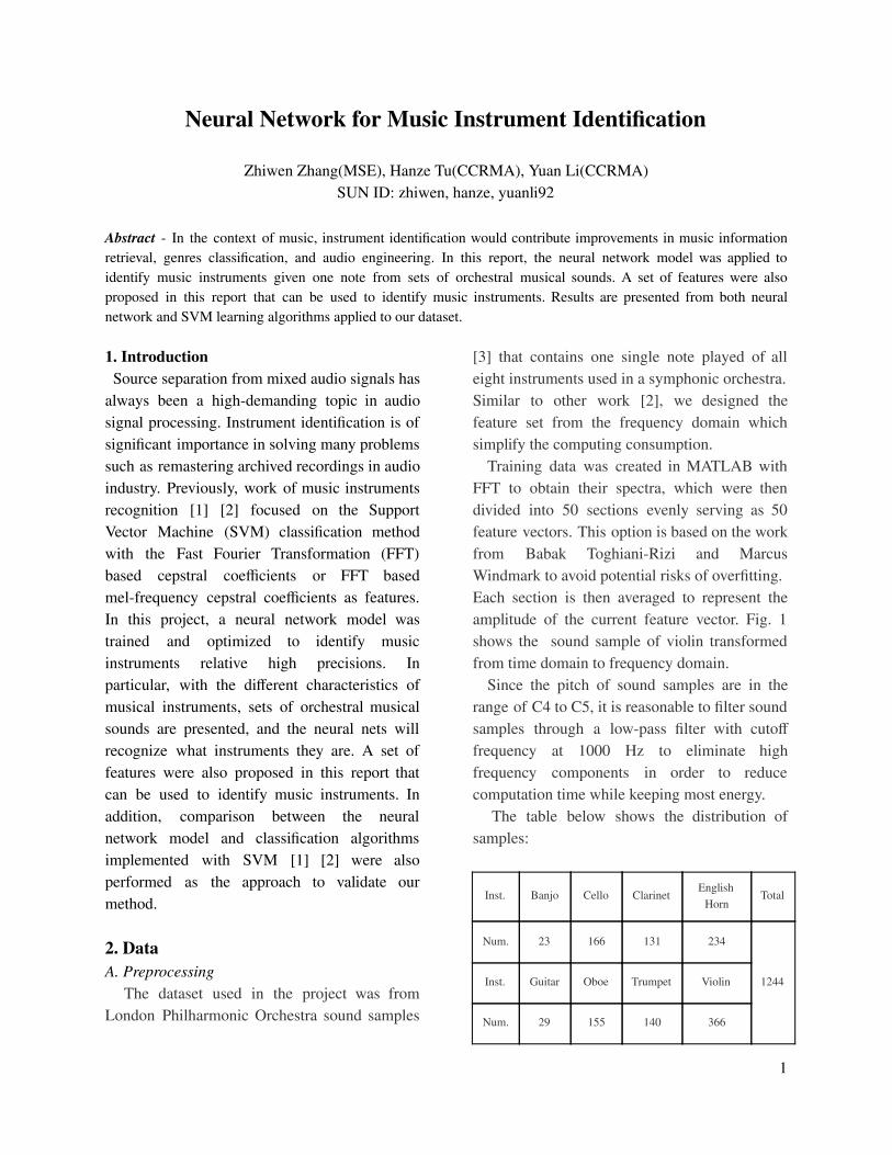
Neural Network for Music Instrument Identi§cation Zhiwen Zhang(MSE), Hanze Tu(CCRMA), Yuan Li(CCRMA) SUN ID: zhiwen, hanze, yuanli92 Abstract - In the context of music, instrument identi§cation would contribute improvements in music information retrieval, genres classi§cation, and audio engineering. In this report, the neural network model was applied to identify music instruments given one note from sets of orchestral musical sounds. A set of features were also proposed in this report that can be used to identify music instruments. Results are presented from both neural network and SVM learning algorithms applied to our dataset. 1. Introduction Source separation from mixed audio signals has always been a high-demanding topic in audio signal processing. Instrument identi§cation is of signi§cant importance in solving many problems such as remastering archived recordings in audio industry. Previously, work of music instruments recognition [1] [2] focused on the Support Vector Machine (SVM) classi§cation method with the Fast Fourier Transformation (FFT) based cepstral coeªcients or FFT based mel-frequency cepstral coeªcients as features. In this project, a neural network model was trained and optimized to identify music instruments relative high precisions. In particular, with the di©erent characteristics of musical instruments, sets of orchestral musical sounds are presented, and the neural nets will recognize what instruments they are. A set of features were also proposed in this report that can be used to identify music instruments. In addition, comparison between the neural network model and classi§cation algorithms implemented with SVM [1] [2] were also performed as the approach to validate our method. 2. Data A. Preprocessing The dataset used in the project was from London Philharmonic Orchestra sound samples [3] that contains one single note played of all eight instruments used in a symphonic orchestra. Similar to other work [2], we designed the feature set from the frequency domain which simplify the computing consumption. Training data was created in MATLAB with FFT to obtain their spectra, which were then divided into 50 sections evenly serving as 50 feature vectors. This option is based on the work from Babak Toghiani-Rizi and Marcus Windmark to avoid potential risks of over§tting. Each section is then averaged to represent the amplitude of the current feature vector. Fig. 1 shows the sound sample of violin transformed from time domain to frequency domain. Since the pitch of sound samples are in the range of C4 to C5, it is reasonable to §lter sound samples through a low-pass §lter with cuto© frequency at 1000 Hz to eliminate high frequency components in order to reduce computation time while keeping most energy. The table below shows the distribution of samples: Inst. Banjo Cello Clarinet English Horn Total Num. 23 166 131 234 1244 Inst. Guitar Oboe Trumpet Violin Num. 29 155 140 366 1
Transcript of Neural Network for Music Instrument...
Neural Network for Music Instrument Identi�cation
Zhiwen Zhang(MSE), Hanze Tu(CCRMA), Yuan Li(CCRMA) SUN ID: zhiwen, hanze, yuanli92
Abstract - In the context of music, instrument identi�cation would contribute improvements in music information retrieval, genres classi�cation, and audio engineering. In this report, the neural network model was applied to identify music instruments given one note from sets of orchestral musical sounds. A set of features were also proposed in this report that can be used to identify music instruments. Results are presented from both neural network and SVM learning algorithms applied to our dataset.
1. Introduction Source separation from mixed audio signals has
always been a high-demanding topic in audio signal processing. Instrument identi�cation is of signi�cant importance in solving many problems such as remastering archived recordings in audio industry. Previously, work of music instruments recognition [1] [2] focused on the Support Vector Machine (SVM) classi�cation method with the Fast Fourier Transformation (FFT) based cepstral coe�cients or FFT based mel-frequency cepstral coe�cients as features. In this project, a neural network model was trained and optimized to identify music instruments relative high precisions. In particular, with the di�erent characteristics of musical instruments, sets of orchestral musical sounds are presented, and the neural nets will recognize what instruments they are. A set of features were also proposed in this report that can be used to identify music instruments. In addition, comparison between the neural network model and classi�cation algorithms implemented with SVM [1] [2] were also performed as the approach to validate our method.
2. Data A. Preprocessing
The dataset used in the project was from London Philharmonic Orchestra sound samples
[3] that contains one single note played of all eight instruments used in a symphonic orchestra. Similar to other work [2], we designed the feature set from the frequency domain which simplify the computing consumption.
Training data was created in MATLAB with FFT to obtain their spectra, which were then divided into 50 sections evenly serving as 50 feature vectors. This option is based on the work from Babak Toghiani-Rizi and Marcus Windmark to avoid potential risks of over�tting. Each section is then averaged to represent the amplitude of the current feature vector. Fig. 1 shows the sound sample of violin transformed from time domain to frequency domain.
Since the pitch of sound samples are in the range of C4 to C5, it is reasonable to �lter sound samples through a low-pass �lter with cuto� frequency at 1000 Hz to eliminate high frequency components in order to reduce computation time while keeping most energy.
The table below shows the distribution of samples:
Inst. Banjo Cello Clarinet English
Horn Total
Num. 23 166 131 234
1244 Inst. Guitar Oboe Trumpet Violin
Num. 29 155 140 366
1

Table 1. the distribution of instrument samples
Figure 1. Sound sample of trumpet in time domain
and frequency domain( Discard half of points)
B. Feature Extraction for Dataset Dataset #1 :
This dataset contains 1244 labeled samples in
total, each donates 50 features (the after
preprocessing dataset) .
Dataset #2 : Based on Dataset #1, apply low-pass �lter with
cuto� frequency at 900Hz to �lter all frequency
components above 900Hz for all samples. Since
Dataset #1 has samples in the range of 1-1000
Hz, it’s inspiring to study the importance of 10%
less information, especially under the condition
that dealing with massive input data.
Dataset #3: Clark [4] performed a study on the importance
of the di�erent parts of a tone for human
recognition and concluded that having only the
attack resulted in a good accuracy of recognizing
most instruments. Then, in this report, the attack
feature was extracted and the importance of the
attack was analyzed by having only the attack in
the Dataset #3.
The extraction of each sample was performed
in time domain before the preprocessing, by
�nding the onset point where this energy was 10
dB over the signal average as mentioned in
Bello ‘s work [5] (attack period has a �xed
transient length 80 ms). Then partition each
attack sample into 50 sections to get 50 features
as well.
3. Models In this section, di�erent models and techniques
were tested with respect to dimensions of input
data and computation cost. Eventually, Neural
Network using Tensor�ow[7] and SVM were
applied to this project.
A. Neural Network In our multi-layer perceptron model, the input
layer reads in 50 features contributed by an
instrument sample. The hidden layer with an
sigmoid activation function has 30 hidden nodes,
reducing the feature dimension to 30. The
activation function for the output layer is the
softmax function, which gives a probability
distribution over output labels.
To Train our model, de�ne the objective to be
minimizing the cross-entropy. Cross-entropy (eq.
1) measures how ine�cient our predictions are
for describing the truth in.
Eq. (1 )
Where y is the predicted probability distribution,
and y′is the true distribution (the one-hot
instrument labels).
Then, instead of using the simple Gradient
2

Descent optimization method, the neural
network uses Adam Optimizer of Tensor�ow
[7], which is implemented based on Diederik
Kingma and Jimmy Ba ’s Adam algorithm [8] to
control the learning rate. Adam algorithm has
advantages over the simple Gradient Descent
Optimizer. Foremost is that it uses momentum,
which is the moving averages of the parameters.
Figure 2 shows the neural network model used
for the project.
Figure 2. Neural Network Structure
B. Support Vector Machines (SVMs ) SVMs are a set of supervised learning methods
widely used for classi�cation , regression and
outliers detection . In addition, SVMs are very
versatile that can be adapted and speci�ed for
di�erent decision functions using di�erent
kernels. In this project, RBF Kernel is chosen to
perform the task, which is well known in Signal
Processing as a tool to smooth the data.
Eq. (2)
The RBF kernel on two samples x and x',
represented as feature vectors in the input space.
And the parameter grid contains the several
chosen value for Penalty parameter C of the
error term and the Kernel coe�cient for RBF
kernel.
4. Results
A. Tensor�ow Neural Network Fig.3 shows the curve of the cross-entropy
versus training iterations with the learning rate
of 0.001.
Figure 3. Cross-entropy versus training iterations
with learning rate 0.001
The neural network model was trained with the
datasets with 20%-20%-60% split on the test set,
validation set, and training set. Generalization
error, validation error, and training error is
shown below:
Figure 4. Generalization error, validation error,
and training error of three datasets
It is noticeable from Fig. 4 that best results
came from Dataset #1 with the test accuracy of
87%, The training and validation error over
iterations is shown below:
3

Figure 5. Training error, validation error vs. Training
Iterations for Dataset#1
To visualize the learning process of our model,
Tensor�ow built in visualization tool Tensorboard is
used, which is able to display the weights and biases
in di�erent layers during the training process and
help to check if the neural network model actually
learned something.
Since the Dataset#1 gives the best model after
training, it’s now helpful to show how the weights
and biases change during the training process in the
hidden layer and the output layer.
Figure 6-a and Figure 6-b shows the change of
weight distribution of the hidden layer and the output
layer, respectively. After 8000 taining steps, weights
ranges from -8 to 8 approximately in the hidden layer
and it ranges from -6.5 to 7 approximately in the
output layer.
Figure 6-a Dataset #1: Weights-Training iterations
Histogram for the hidden layer
Figure 6-b Dataset #1: Weights-Training iterations
Histogram for the prediction layer
Figure 6-c and Figure 6-d shows the change of
biases of the hidden layer and the output layer,
respectively. After 8000 taining steps, biases change
from 0 to a range of -3 to 4.5 approximately in the
hidden layer and to a range of -0.4 to 0.85
approximately in the output layer.
Figure 6-c Dataset #1: Bias-Training iterations
Histogram for the output layer
Figure 6-d Dataset #1: Bias-Training iterations
Histogram for the output layer
4
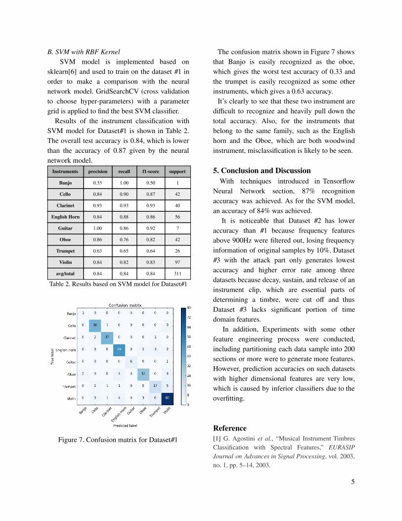
B. SVM with RBF Kernel SVM model is implemented based on
sklearn[6] and used to train on the dataset #1 in order to make a comparison with the neural network model. GridSearchCV (cross validation to choose hyper-parameters) with a parameter grid is applied to �nd the best SVM classi�er.
Results of the instrument classi�cation with SVM model for Dataset#1 is shown in Table 2. The overall test accuracy is 0.84, which is lower than the accuracy of 0.87 given by the neural network model.
Instruments precision recall f1-score support
Banjo 0.33 1.00 0.50 1
Cello 0.84 0.90 0.87 42
Clarinet 0.93 0.93 0.93 40
English Horn 0.84 0.88 0.86 56
Guitar 1.00 0.86 0.92 7
Oboe 0.86 0.76 0.82 42
Trumpet 0.63 0.65 0.64 26
Violin 0.84 0.82 0.83 97
avg/total 0.84 0.84 0.84 311
Table 2. Results based on SVM model for Dataset#1
Figure 7. Confusion matrix for Dataset#1
The confusion matrix shown in Figure 7 shows that Banjo is easily recognized as the oboe, which gives the worst test accuracy of 0.33 and the trumpet is easily recognized as some other instruments, which gives a 0.63 accuracy.
It’s clearly to see that these two instrument are di�cult to recognize and heavily pull down the total accuracy. Also, for the instruments that belong to the same family, such as the English horn and the Oboe, which are both woodwind instrument, misclassi�cation is likely to be seen.
5. Conclusion and Discussion
With techniques introduced in Tensor�ow Neural Network section, 87% recognition accuracy was achieved. As for the SVM model, an accuracy of 84% was achieved.
It is noticeable that Dataset #2 has lower accuracy than #1 because frequency features above 900Hz were �ltered out, losing frequency information of original samples by 10%. Dataset #3 with the attack part only generates lowest accuracy and higher error rate among three datasets because decay, sustain, and release of an instrument clip, which are essential parts of determining a timbre, were cut o� and thus Dataset #3 lacks signi�cant portion of time domain features.
In addition, Experiments with some other feature engineering process were conducted, including partitioning each data sample into 200 sections or more were to generate more features. However, prediction accuracies on such datasets with higher dimensional features are very low, which is caused by inferior classi�ers due to the over�tting.
Reference [1] G. Agostini et al. , “Musical Instrument Timbres Classi�cation with Spectral Features,” EURASIP Journal on Advances in Signal Processing , vol. 2003, no. 1, pp. 5–14, 2003.
5

[2] J. Marques and P. J. Moreno, “A Study of Musical
Instrument Classi�cation using Gaussian Mixture
Models and Support Vector Machines,” Cambridge
Research Laboratory Technical Report Series CRL,
Cambridge, MA, Apr. 1999.
[3] London Philharmonic Orchestra Sound Samples
[Online] Available:
http://www.philharmonia.co.uk/explore/sound_sampl
es
[4] M. Clark et al. “Preliminary Experiments on the
Aural Signi�cance of Parts of Tones of Orchestral
Instruments and on Choral Tones,” Journal of the Audio Engineering Society , vol. 11, no. 1, pp. 45–54,
Jan. 1963.
[5] J. P. Bello et al. , “A tutorial on onset detection in
music signals,” Speech and Audio Processing , IEEE
Transactions on, vol. 13, no. 5, pp. 1035–1047, 2005.
[6] Scikit-Learn [Online] Available:
http://scikit-learn.org/stable/modules/svm.html#svm
[7] Tensor�ow [Online] Available:
https://www.tensor�ow.org/
[8] D. Kingma and J. Ba, “Adam: A Method for
Stochastic Optimization,” The 3rd International
Conference for Learning Representations, San Diego,
Dec. 2014.
6