HAL Id: hal-03096952https://hal-centralesupelec.archives-ouvertes.fr/hal-03096952

Submitted on 5 Jan 2021

HAL is a multi-disciplinary open accessarchive for the deposit and dissemination of sci-entific research documents, whether they are pub-lished or not. The documents may come fromteaching and research institutions in France orabroad, or from public or private research centers.

L’archive ouverte pluridisciplinaire HAL, estdestinée au dépôt et à la diffusion de documentsscientifiques de niveau recherche, publiés ou non,émanant des établissements d’enseignement et derecherche français ou étrangers, des laboratoirespublics ou privés.

Transient-based fault identication algorithm usingparametric models for meshed HVDC grids

P. Verrax, A. Bertinato, Michel Kieffer, B. Raison

To cite this version:P. Verrax, A. Bertinato, Michel Kieffer, B. Raison. Transient-based fault identication algorithm usingparametric models for meshed HVDC grids. Electric Power Systems Research, Elsevier, 2020, 185,pp.106387. 10.1016/j.epsr.2020.106387. hal-03096952

Transient-based fault identication algorithm

using parametric models for meshed HVDC grids

P. Verraxa,b,∗, A. Bertinatoa, M. Kieera,b, B. Raisona,c

aSuperGrid Institute, 23 rue Cyprian, BP 1321, 69611 Villeurbanne Cedex, FrancebL2S, Univ Paris-Sud, CNRS, CentraleSupelec, Univ Paris-Saclay, Gif-sur-Yvette F-91190, France

cUniv. Grenoble Alpes, CNRS, Grenoble INP*, G2Elab, 38000 Grenoble, France. (* Institute of Engineering Univ. Grenoble Alpes)

Abstract

This paper addresses the problem of fault identication in meshed HVDC grids once an abnormal behavior has beendetected. A parametric single-ended fault identication algorithm is proposed. The method is able to determine whetherthe line monitored by a relay is faulty or not using a very short observation window. When a fault is suspected, theproposed algorithm estimates the fault distance and impedance using a parametric model describing the voltage andcurrent evolution just after the fault occurrence. This model combines physical and behavioral parts to represent thefault propagation and to account for ground eects and various losses. The identication of the faulty line is then basedon the size of the condence region of the obtained estimate. The performance of the algorithm for a three-node meshedgrid is studied using Electro-Magnetic Transient (EMT) simulations. On the considered grid model, the current andvoltage need to be observed during less than 0.2ms to get a suciently accurate estimate of the fault characteristics andidentify consistently the faulty line.

Keywords: HVDC, Multi-terminal, protection, fault detection, fault localization, parameter identication

1. Introduction

In the future, Multi-Terminal high-voltage Direct-Current(MTDC) grids are likely to act as a backbone to the ex-isting AC network, providing better interconnection overlarge distances between renewable energy sources and con-sumption area as well as integration of large oshore windpower plants [1]. Among the several technical and non-technical barriers still to overcome for the development ofHigh-Voltage Direct-Current (HVDC) meshed grids, theprotection of the lines is seen as one of the most chal-lenging [2]. Protection strategies and breaker technologiesdeveloped in the case of High Voltage Alternative Cur-rent (HVAC) grids cannot be directly translated to HVDCgrids, since, for example, faults on an HVDC line, do notlead to a zero-crossing of the current, which makes thefault clearance more dicult.

The main tasks of a protection strategy include faultdetection, faulty component identication, and tripping ofthe breakers, see [3]. If the breakers are triggered beforethe faulty component is identied, so that a large part ofthe grid is de-energized, one refers to as a non-selectivefault clearing strategy, see for instance [4]. On the op-posite, selective fault clearing strategies consist in identi-fying the faulty component so that only the correspond-

∗Corresponding authorEmail address: paul.verrax@supergrid-institute.com

(P. Verrax)

ing breakers are triggered, which is considered preferablesince this minimizes the impact of the fault on the grid.In such a strategy, breaking modules located at the end ofeach line are responsible for the protection of their respec-tive line, see Figure 1. Overall, protection strategies mustbe reliable [5], i.e., they must lead to an isolation of theprotected line only when needed and must be immune tochanges caused by normal operations on the grid. Finally,protection algorithms must operate fast enough to copewith Direct Current Circuit Breaker (DCCB) capabilities.DC inductances located between each relay and the bus-bar are generally considered in the literature to slow downthe rise of the current. In grids involving overhead lines,however, the inductive behavior of the lines may enableto omit such inductances, which is considered preferableregarding the cost and dynamic behavior of the grid [6].Such an approach requires fast fault identication as wellas fast breakers. The use of hybrid DCCB is seen as anadvantageous compromise between the operating time andthe breaking capabilities of the breakers, see [7]. The typ-ical available time to detect and identify the fault is thenless than a millisecond. This makes use of communica-tion between distant protection devices not suitable, sincesuch communications induces several milliseconds of delay,as shown in [8]. Hence, a selective protection scheme re-quires a single-ended (non-unit) algorithm [3] ensuring se-lectivity, i.e., able to discriminate between internal faults,occurring on the protected line and external faults, occur-

Preprint submitted to Electric Power Systems Research January 5, 2021

Converter 1

Converter 3

Converter 2

Line breaker

Converter breaker

DC reactor

Figure 1: Example of a three-node MTDC network; DC reactors areassumed available in most state-of-the-art fault identication algo-rithms, whereas in the proposed approach they are not required toachieve selective fault identication.

ring elsewhere in the grid.This paper, introduces a protection algorithm to be

used in a primary selective strategy1. We propose a novelsingle ended protection algorithm able to detect and iden-tify faults occurring on transmission lines. Each relay em-beds an analytical parametric model of the evolution ofthe current and voltage after the occurrence of a fault, de-pending on a set of physical fault parameters. When afault is suspected, an iterative maximum-likelihood (ML)estimate of the fault parameters is evaluated from the mea-surements available at the relay. The estimated fault pa-rameters and their condence intervals are exploited todetermine whether or not a fault actually occurred on theprotected line. O-line transient simulations in EMTP-RV [10, 11] show that the proposed algorithm can identifymost of internal faults from measurements collected over atime window of less than 0.2 ms after the detection of anabnormal behavior on the line and is immune to faults onneighboring lines. Contrary to most existing approaches,extra inductances are not required to distinguish betweenfaults occurring on the protected line and elsewhere.

Section 2 provides an overview of existing protectionalgorithms. Section 3 presents the problem formulationand the proposed approach. The modeling of the faultbehavior is detailed in Section 4 and the estimation algo-rithm for the fault parameters is described in Section 5.The identication process using condence intervals is de-tailed in Section 6. Simulation results are presented inSection 7, before drawing some conclusions and future re-search directions in Section 8.

2. Related work

This section overviews existing detection, identica-tion, and localization methods, focusing on single-endedalgorithms. More extensive reviews of protection schemes

1In case of fault identication failure, a non-selective strategy suchas presented in [9] can be applied as back up.

and existing technologies can be found in [12], [13], and[14].

2.1. Amplitude-based methods

Fault behavior is generally associated with high vari-ation rates in both current and voltage. Various meth-ods using thresholds on voltage and/or current derivativeshave been proposed.

A general method to tune such thresholds is developedin [15] using a reduced grid model instead of extensivetransient response simulations. In [16], the rate of changeof voltage across the DC reactors is used to detect andidentify the fault. The Multi Modular Converters (MMC)arm inductances, along with large DC reactors (200 mH),are used to tune the detection thresholds.

Regarding current-based algorithm, [17] proposed a three-stage method, rst detecting peaks in the deviation of thecurrent from a moving average, then comparing the cur-rent value with previous highest values and nally com-paring the current deviation to a predetermined thresholdto ensure selectivity. Methods based on voltage and cur-rent derivative along with over-current methods are com-pared in [18], which shows that a combined criterion couldachieve selective fault detection. A criterion combiningthe voltage and current derivatives, as well as the currentsecond-order derivative is proposed in [19]. Additionally,the concept of critical fault resistance is used to detect onlyfaults that would lead to current rise higher than 2 p.u.

The aforementioned algorithms share the assumptionof the presence of rather large inductances at the end ofeach line, see Figure 1, generally required to limit the riseof current and achieve selectivity. Nevertheless, such in-ductances are costly and may deteriorate the dynamic per-formance of the system and cause instability [6]. Moreover,such methods rely on critical thresholds to ensure both de-pendability and selectivity.

2.2. Model-based methods

Dierent techniques have tried to benet from moreaccurate traveling wave models describing the evolution ofcurrent and voltage when a fault appears in a line.

In [20], the S-transform of the voltage is used to detectthe arrival times of the traveling waves. Along with thepolarities of the waves, this allows oneto locate the faulton a given line. In a similar fashion, but in the context ofAC transmission, [21] uses multiple traveling wave arrivaltimes to spot the pattern of the reections between the ob-servation point and the fault. The method is then able tolocate a fault on a line inserted in a meshed grid. Severaltraveling wave arrival times (about a dozen) need to beacquired, which limits the speed of the method. In thosetwo methods, the key challenges consist in being able tospot accurately the wave fronts, and in being able to dis-tinguish waves due to reection at the fault from waves dueto other reections in the grid. Note that both algorithmsalso assume that the fault has already been detected on aspecic line and focus on the fault accurate localization.

In [22], the Bergeron method is applied to reconstructthe distribution of the voltage along a healthy line usingvoltage and current measurements at the end of the line.The computed voltage distribution at both ends are hencecorrect up to the point where the line is faulty. Assumingsynchronized communication is available between the re-lays, the fault location can be computed as the point wherethe reconstructed voltage from both sides are matching.Such a point can be found using a least-squares algorithm.Still using synchronized data, [23] developed a dynamicstate estimation algorithm for fault localization in AC sys-tems. A chi-square condence test is employed to validatethe results of the fault location estimation. Nevertheless,as mentioned earlier, the use of communications, especiallyto get synchronized data, is not suitable for fast fault de-tection due to measurement transmission delays, see forinstance [8].

The concept of electromagnetic time reversal, used in[24], takes advantage of the time reversal invariance of elec-tromagnetic equations such as the telegraph equations. Bycomparing, in reversed time, the recorded voltage at a sta-tion and a simulated voltage transient at a given observa-tion point, one can estimate the fault location. Neverthe-less, the method is meant as a localization algorithm andassumes information on the fault type from the breakersis available as well as more than 5 ms long measurementwindow.

When the system is based on voltage source converterswith large shunt capacitance, [25] showed that this capac-itance could be accurately identied in the case of inter-nal faults using local voltage and current measurements.On the contrary, external faults would lead to an erro-neous identication. In [26], a rational approximation ofthe characteristic admittance of the line is used to detectthe rst incident wave of the current. Selective detectionis then achieved using a predetermined static thresholdon the incident wave, still assuming the presence of DCreactors to distinguish external disturbances.

A multiple behavioral model-based approach has beendeveloped in [27]. Universal line models are derived for anite set of possible fault cases. These models are com-bined in a bank of Kalman lters used to perform the faultidentication. Measurements from the relay are then com-pared to the predictions obtained from the lters. The bestpredicting lter provides an estimate of the fault charac-teristics. This technique requires considering many ltersso as to be able to identify faults with a large variety ofcharacteristics, see [27].

Model-based algorithms are hence considered for faultlocalization as well as identication. Nevertheless, ndinga good trade-o between quick detection and identicationand accurate (therefore complex) estimation of the faultcharacteristics is still challenging.

3. Problem formulation and proposed approach

This section describes the problem formulation andprovides an overview of the proposed approach.

3.1. Problem formulation

Consider an MTDC grid described by a graph G =(V, E), where E is a set of edges, representing the linesconnecting pairs of nodes represented by the vertices in V.The nodes may consist of converter stations or other equip-ments such as sensors, relays, etc. Transmission lines canbe overhead lines (OHL), underground cables, or a com-bination of both. Consider some vertex q ∈ V connectedto nq lines. Within the node represented by q, each line isassumed to be monitored by some fault identication de-vice (FID) in charge of determining whether the line underprotection is faulty. Each node contains thus nq FID, eachdedicated to an incoming line.

Consider a fault occurring at some time instant tf on agiven line e = (q, q′) ∈ E of length dqq′ connecting stationsq and q′ of the grid. The distance of the fault to stationsq and q′ along the line e is df,q and df,q′ , respectively with

df,q + df,q′ = dqq′ . (1)

The fault is assumed to be characterized by its pole-to-ground or pole-to-pole impedance Zf depending on thetype of fault, considered constant during the time intervalof interest in the order of a millisecond. The vector of pa-rameters describing a fault is thus p = (e, df,q, df,q′ , Zf, tf)

T.

Assume that the FID of station q monitoring line e ac-quires at a frequency f voltage and current measurements(vq,e (t) , iq,e (t)) at the end of e connected to q. Usingtools presented, e.g., in [17], the FID is able to determinewhether the grid behaves normally or not. Let td,q > tfdenotes the time instant at which an abnormal behavioris detected at station q.

Once such abnormal behavior has been detected, theFID has to determine, using all available information, whetheror not the fault occurred in the line under protection.

3.2. Overview of the proposed approach

In the proposed approach (see Figure 2), an ML esti-mate of the vector of parameters p characterizing the faultis evaluated using the voltage and current measurements(vq,e (t) , iq,e (t)). For that purpose, a parametric model ofthe voltage and current evolution at node q is considered incase of fault occurrence. This model depends on the char-acteristics of the grid, which are supposed known, and onthe unknown vector of fault parameters p. For a givenvalue of p, the output at time t of the parametric model isdenoted as

(vmq,e (p, t) , imq,e (p, t)

). As will be seen in Sec-

tion 4, the considered model combines a knowledge-basedmodel derived from physical principles and a behavioralmodel used to take into account additional eects such asthe soil resistivity.

Sensors

Model M(p)(Section 4)

Parameter tuning(Section 5)

Decision logic(Section 6)

−+

Confidence region

vq,e(t), iq,e(t)

vmq,e(p, t), imq,e(p, t)

p

Estimated parameters

Figure 2: Overview of the proposed fault parameter vector estima-tion approach. Subscripts q and e are omitted to lighten the nota-tions.

Assuming that the fault actually occurred on the linee, the FID evaluates an estimate p of the fault param-eter vector p. This estimation is performed recursively:p is updated when new measurements are available. Theparameter estimation algorithm is detailed in Section 5.For each estimated parameter vector p, an approximatecondence region is evaluated. An hypothesis test is thenconsidered involving the estimate p and its condence re-gion to determine whether a fault actually occurred in theline e. The hypothesis test may conclude that the faultaects line e, in which case a selective clearing strategy istriggered. When it is unable to conclude, the FID waitsfor the availability of additional measurements to updatep and the associated condence region. Once enough mea-surements have been made available without allowing theFID to conclude, the fault, if it exists, is deemed to belocated elsewhere in the grid. The hypothesis test and thedecision logic are detailed in Section 6.

4. DC Fault analytic modeling

This section presents the model introduced to describethe evolution of the current and voltage measured at theend of a monitored line aected by a fault. The consid-ered model combines a knowledge-based model, involvingthe telegraph equations, described in Section 4.1, and a be-havioral model, to account for the eect of soil resistivity,described in Section 4.2. This two-stages model approachis summarized in Figure 3. The output of the knowledge-based model serves as input of the behavioral model. Tosimplify presentation, the case of an asymmetric monopolewith single conductor overhead lines is considered. Theapproach can be extended to the case of underground ca-bles or lines consisting of several types of interconnectedtransmission lines.

4.1. Physical modeling

This section describes the knowledge-based part of themodel presented in Figure 3.

Physicalmodel

Behavioralmodel

Line parameters

Station parameters

Grid topology

Soil resistivity

Faultparameters p ym,0(t,p) ym,g(t,p, ρ)

ρ

Figure 3: Combined knowledge-based (physical) and behavioralmodel

4.1.1. Description of traveling waves

Consider a line e = (q, q′) belonging to a meshed grid aspresented in Figure 1. The evolution of current and volt-age measured at a given point of e can be modeled usingtraveling waves, as shown in [28]. Along the line, currentand voltage satisfy the telegraph equations, expressed inthe Laplace domain as

∂2V

∂x2= Z(s)Y (s)V (x, s) (2)

∂2I

∂x2= Y (s)Z(s)I(x, s), (3)

where Z(s) = R+ sL and Y (s) = G+ sC are the transferfunctions of the distributed series impedance and shuntadmittance, respectively. When a fault occurs, two volt-age and current waves Vq,1 and Vq′,1 starting from the faultlocation travel along the line towards node q and q′, respec-tively. They undergo a certain attenuation and distortionaccording to some propagation function H

Vq,1 (s, dq) = H (s, dq)Vinit(s) (4)

Vq′,1 (s, dq′) = H (s, dq′)Vinit(s), (5)

where Vinit is the initial surge at fault location and (dq, dq′)are the traveled distances from the fault towards the twostations, respectively. H can be expressed, for a traveleddistance d along the line, as

H (s, d) = exp(−√Y (s)Z(s)d

). (6)

Any voltage traveling wave V has an associated currentwave dened as

I(s, d) = Z−1c (s)V (s, d),

where the characteristic impedance Zc is

Zc (s) =√Z(s)/Y (s). (7)

When a change of propagation medium occurs (typi-cally at the junction between a line and a station), theincident wave Vf gives rise to a transmitted and a reectedwave, Vt and Vr respectively. The associated voltage Vtotat the media change point is then

Vtot = Vt = Vf + Vr

= (1 +K)Vf

= TVf, (8)

FaultStation q Station q′ Station q′′Station q′′df,q df,q′dq′′q dq′q′′

Vq,1Vq′,1

tf

td,q

td,q′time

Figure 4: Example of a Bewley lattice diagram.

where the transmission and reection coecients T andK depend on the characteristic impedances of the me-dia. For a wave traveling from a medium of characteristicimpedance Z1 to a medium of characteristic impedanceZ2, one has

K1→2 =Z2 − Z1

Z2 + Z1and T1→2 =

2Z2

Z2 + Z1. (9)

If the junction connects more than two conductors, thetransmission and reection coecients must be adaptedaccordingly. Consider a wave from medium 1 of charac-teristic impedance Z1 propagating to n− 1 media of char-acteristic impedance Z2, . . . , Zn. The reection coecientas seen from medium 1 becomes

K1→2...n =1/Z1 −

∑n`=2 1/Z`∑n

`=1 1/Z`. (10)

Similarly, the transmission coecient from medium 1 to `is

T1→` = 1 +K1→2...n =2/Z1∑n`=1 1/Z`

. (11)

Using the reection and transmission coecients as wellas the propagation functions as described before one canevaluate the incident, reected, and transmitted travelingwaves with the help of a Bewley lattice diagram [29]. Suchdiagram is presented in Figure 4 for the case of a three sta-tion network, as presented in Figure 1, connecting stationsq, q′, and q′′. The station q′′ is represented on both sidesof the diagram.

4.1.2. Lossless line model and converter stations

This section describes how time-domain expression ofthe traveling waves are obtained for a line e connectingtwo power stations q and q′ represented in Figure 1. Forthat purpose, a lossless line model is considered and theMMC are represented by RLC equivalents. The eect ofsoil resistivity in the ground return path is temporarilyneglected, so that the distributed series impedance Z andshunt admittance Y in (6) depend only on the overheadline characteristics and do not vary signicantly with thefrequency, see Appendix Appendix A.

To describe the transient behavior of voltage and cur-rent once a fault has occurred, the series resistance R andshunt conductance G are neglected compared to the eectsof the series inductance L and shunt capacitance C. Thevalidity of this assumption is investigated in Appendix Ap-pendix A. With this lossless model, (6) and (7) become

H(s) = exp(−s√LCd

)(12)

andZc =

√L/C. (13)

Modular Multilevel Converters (MMC) are consideredwithin each station. If the current increases to 2 p.u.,power electronics within the MMC will protect by auto-blocking, see [30]. When considering only the two or threerst incident, reected, and transmitted waves due to thefault, it is reasonable to consider auto-blocking as inactiveat the arrival times of those waves. This is further detailedin Appendix Appendix B. With this assumption, the RLCmodel

Zmmc (s) = Rmmc + sLmmc +1

sCmmc

(14)

for the MMC introduced in [31] can be employed. Thefault may be represented by a voltage source in series withan impedance Zf between ground and the fault locationconnected at the fault instant tf. The fault impedanceaccounts for dierent eects such as the electric arc, thetower grounding impedance, and the resistance of addi-tional unknown objects in the current path. Here, as in[32], these eects are described considering a single un-known fault resistance, i.e., Zf = Rf. Consequently, thefault leads to the initial surge at the fault location

Vinit (s, tf, Zf) = −vbfZc

Zc + 2Rf

exp (−stf) . (15)

The voltage source has an amplitude opposite to the volt-age vbf at the fault location just before its occurrence.Note that vbf is not available at tf. Nevertheless, assum-ing steady-state conditions line just before tf, voltage andcurrent along the line may be described by telegraph equa-tions in steady state

∂2V

∂x2= RGV. (16)

Typically, the values of R and G are small enough, see Sec-tion 7, to neglect the variations of the voltage along lines,even of several hundreds of kilometers long. Consequently,vbf can be approximated by the steady-state voltage v

(t−d)

measured at the relay just before the fault detection.Hence knowing the characteristics of the dierent lines,

stations, and the topology of the grid one can establish theexpressions in the Laplace domain for any traveling waves.For example, considering a typical faulty line e connectingstations q and q′ of a grid such as that represented inFigure 1, the evolution of the current and voltage at stationq has to account for several traveling waves:

due to the rst incident wave from the fault to sta-tion q; this wave is reected by station q and by thefault (plain blue lines in Figure 4),

due to the rst incident wave from the fault to sta-tion q′, reected by station q′, and transmitted bythe fault (dashed red lines in Figure 4),

due to the transmission of the incident waves to otherlines of the grid or which have been transmitted sev-eral times by the fault (dashed blue and green linesin Figure 4).

Consider rst the traveling waves represented by the solidblue lines in Figure 4. The nth forward and return wavesat the station q due the reections at the fault locationcan be expressed as a function of the fault parameters pas

Vf,n(s,p) = (KqKf)n−1H (s, df,q)

2n−1Vinit (s, tf)

Vr,n(s,p) = KqVf,n (s,p)

(17)where Kq is the reection coecient from the line to thestation q and Kf is the reection coecient at the fault,both given by (10).

Consider now the traveling waves represented by thedashed red lines in Figure 4. The rst incident wave fromthe fault to station q′ (red lines in Figure 4) is reected bystation q′ and transmitted through the fault. This trans-mitted wave can be described at the station q as

V ′f,n(s,p) = Kq′TfH (s, 2dqq′ − df,q)Vinit (s, tf)

V ′r,n(s,p) = KqV′f,n (s,p)

(18)

where Kq′ is the reection coecient from the line to thestation q′ and Tf is the transmission coecient at the fault,given by (11).

Using the previous methodology, one can then get backto temporal domain expressions using inverse Laplace trans-form. Examples of time-domain expressions for the rstwave (17) at station q are

vf,1(t) = − vbfRf

Zc + 2Rf

u (t− td,q) (19)

and

vr,1(t) =2√Cmmc vbf Zc

2

(Zc + 2Rf)Asinh

((t− td,q) A

4√Cmmc Lmmc

)× exp

(− (2Rmmc + Zc) (t− td,q)

4Lmmc

)u (t− td,q)

(20)

where A =√Cmmc(2Rmmc + Zc)2 − 16Lmmc is a scalar

coecient depending only on the line surge impedance andthe MMC parameters. The time td,q is the detection timecorresponding to the arrival time of the rst wave at sta-tion q. It can be expressed as a function of the fault time tf,

the fault distance df,q, and the wave speed cw = 1/√LC;

td,q = tf +df,qcw

. (21)

Similar expressions can be obtained for the other wavesdue to reections at the fault and for waves due to reec-tions at other stations. The total voltage at the station isthen the sum of the measured prior fault voltage v(t = t−d,q)and the dierent waves arriving at the station as derivedusing the Bewley diagram, see Figure 4.

vtot(t,p) = v(t−d,q) + vf,1(t,p) + vr,1(t,p) + vf,2(t,p) + . . .(22)

The number of reections that must be taken into accountresults in a trade-o between the complexity and desiredtime validity interval of the model. Since the characteristicimpedance is scalar, the current reaching the MMC fromthe monitored line is deduced from the voltage

itot(t,p) = i(t−d,q)+Z−1c (vf,1(t,p)−vr,1(t,p)+vf,2(t,p) . . . ).

(23)The expressions (19), (20) and (22), (23) depend on theknown characteristics of the grid, and on measured quan-tities such as the detection time as well as the voltageand current just before the occurrence of the fault. Asmentioned in Section 3, these expressions also depend onthe fault parameter vector p = (e, df,q', df,q, Rf, tf)

Twhich

value has to be identied.

4.2. Accounting for the soil resistivity

The knowledge-based model introduced in Section 4.1.1neglects the eect of the soil resistivity. This section in-troduces a behavioral model that supplements the physicalmodel to take into account soil resistivity eects.

Here, the soil resistivity is assumed to be representedby a known constant parameter ρ along the return path ofthe monitored line. While dierent approaches to modelphysically the behavior of the ground exist (see for instance[33]), to the best of our knowledge they do not lead to ananalytic temporal expression of the current and voltagetransient evolution. To account for soil resistivity eects,we supplement the knowledge-based model of Section 4.1.1with a behavioral model, to get a combined model, seeFigure 3.

Assume that ym,0 (p, t) =(vm,0 (p, t)

T, im,0 (p, t)

T)T

is the output of the knowledge-based model in Section 4.1.1,representing the voltage and current at a given point of themonitored line e. Preliminary simulations have shown thatthe soil resistivity impacts the model output ym,0 (p, t)as a low-pass lter. Consequently, the output ym,g =(vm,g (p, t)

T, im,g (p, t)

T)T

of the model accounting for

the eects of the soil resistivity is described as

ym,g(p, ρ, tk) = G(z−1)ym,0 (p, tk) , (24)

with G(z−1) = B(z−1)A(z−1) is a transfer function, where

A(z−1)

= 1− a1z−1 − · · · − ana

z−na (25)

is an auto-regressive part that represents the inductive ef-fect of the soil resistivity, while

B(z−1) = z−nd(b0 + b1z

−1 + · · ·+ bnbz−nb

)(26)

is a exogenous part that takes ym,0 (p, tk) as external in-put. The coecients na and nb are the orders of the poly-nomials A and B respectively, while nd models the input-output delay.

An oine estimation of nd and of the coecients aiand bi may then be performed considering the measure-

ments y(t) =(v (t)

T, i (t)

T)T

for a vector of known fault

parameters p using, e.g., the Electro-Magnetic Transient(EMT) software EMTP-RV [11]. Using (24), the outputsaccounting for the soil resistivity provided by EMTP-RVare assumed to be described by

A(z−1)y (tk) = B(z−1)ym,0 (p, tk) + ε (tk) , (27)

where ε (t) represents the measurement error term and alleects not captured by the model (24). Then, for givenvalues of the fault parameter vector p and of ρ, a least-squares estimate of nd and of the parameters ai, bi hasbeen performed [34].

The coecients of the transfer function G which mod-els the eect of soil resistivity clearly depend on the valueof ρ. Moreover, additional simulations have also evidencedthe impact of the components of the fault parameter vec-tor p, among which the distance to the fault df is the mostimportant. In order to get a behavioral model of the im-pact of the soil resistivity that is valid whatever the faultlocation, one explicitly accounts for df in the parametersai and bi of the model.

Low order models have proven to give a relatively goodt of the simulated voltage and currents from EMTP. Inthe case of a rst order low pass lter, the coecients a1,b0 and nd can be estimated for dierent values of the faultdistance df and a given value of ρ, considering only therst traveling wave generated by a fault.

the following model

am1 (df) = α1,0 + α1,1d−1f + α1,2d

−2f (28)

bm0 (df) = β0,0 + β0,1d−1f + β0,2d

−2f (29)

nmd (df) = Round(ν0 + ν1d

1f + ν2d

2f

)(30)

of the evolution of a1, b0 and nd with df depending on theparameters vectorsα1 = (α1,0, α1,1, α1,2)

T, β0 = (β0,0, β0,1, β0,2)

T

and ν = (ν0, ν1, ν2)Thas been adjusted by least-squares

estimation.A comparison of the output of the complete model with

that of the knowledge-based model is provided in Section 7.The estimation of the lter coecients am1 (df), b

m0 (df), and

nmd (df) is also described.

4.2.1. Other traveling waves

To account for the eect of soil resistivity on othertraveling waves, the distance d in the parameters am1 (d)and bm0 (d) of the model (24) has to represent the sum ofthe traveled distance.

For instance, the rst traveling wave, once it has beenreected by the station and at the fault location, when itreaches again the station, has traveled three times the faultdistance. The combined model output ym,g is obtained byltering the knowledge-based model output ym,0 with alter G which parameters are am1 (3df) and bm0 (3df). Anexample of this approach is provided in Section 7.2.3.

A possible way to model situations where a line spreadsover areas with dierent soil resistivities, is to consider acascade of several lters G, each tuned for subarea as-sumed of constant soil resistivity.

5. Estimation of the fault parameters

In this section, the estimation of the fault parametersis detailed. This step corresponds to the parameter tuning

block of Figure 2 introduced in Section 3 and uses theparametric model described in Section 4.

Consider that an unusual behavior is detected by arelay q monitoring a line e at the time td,q. Assume that

n voltage and current measurements y (t) = (v (t) , i (t))T

have been performed at time tk, k = 1, . . . , n, with t1 6td,q < tn. For a given value of p, one may evaluate the

combined model outputs ym (p, t) = (vm (p, t) im (p, t))T

and evaluate the output error

ey (p, tk) = y (tk)− ym (p, tk) , k = 1, . . . , n. (31)

Assume that, for the true value of the fault parameters p∗,the observed data satisfy

y (tk) = ym (p∗, tk) + ε(tk), k = 1, . . . , n (32)

where εk belongs to a sequence of realizations of indepen-dent random vectors that follows a zero-mean Gaussiandistribution with known covariance matrix

Σ =

(σ2v 0

0 σ2i

), (33)

where σ2v and σ2

i are obtained from the characteristics ofthe voltage and current sensors. The ML estimate of pfrom n observations is

p = arg maxp

π (y (t1) , . . . ,y (tn) |p) , (34)

see [35]. With the considered measurement noise model,evaluating p requires the minimization of the cost function

c(n)(p) = f (n)(p)T(

Σ(n))−1

f (n)(p), (35)

where

f (n) (p) =[(v (t1)− vm (p, t1)) , . . . , (v (tn)− vm (p, tn))

(i (t1)− im (p, t1)) , . . . , (i (tn)− im (p, tn))]T, (36)

andΣ(n) = diag

(σ2v, . . . , σ

2v, σ

2i , . . . , σ

2i

). (37)

In the parameter estimation process, the rst componente of p is assumed xed when trying to decide whether thefault has occurred in the monitored line e or not. More-over, df,q′ can be deduced from (1). Finally the fault occur-rence time tf and the fault distance df,q are related to thedetection time td,q using (21). Since td,q can be measured,only two parameters df,q and Rf are left to be determined.

For a given number of observations n, iterative opti-mization techniques (Gauss-Newton, Levenberg-Marquardt)may be used to build a sequence of parameter estimates

p(n)k+1 = p

(n)k + δ

(n)k , (38)

where δ(n)k is some correction term such that c(n)(p

(n)k+1) <

c(n)(p(n)k ), starting from an initial estimate p

(n)0 . For ex-

ample, with the Gauss-Newton method, one has

δ(n)k = −

(J

(n)Tf

(Σ(n)

)−1

J(n)f

)−1

J (n)T(

Σ(n))−1

f (n),

(39)

where J(n)f is the Jacobian matrix of f (n) with respect to

p evaluated at p(n)k . The computation of the Jacobian

matrix can be done explicitly for the physical model as wellas the combined model, due to their (relative) simplicity.

Assume that after κ iterations (38), n′ measurementsare available, with n′ = n+ ∆n. The cost function c(n)(p)

is updated to c(n′)(p). Then κ new iterates (38) are per-

formed starting from p(n′)0 = p

(n)κ . In practice, κ and the

number of additional measurements ∆n required to updatethe cost function may be tuned to reach a compromise be-tween speed and accuracy of the estimation process.

The estimation algorithm is run until a stopping con-dition is satised, as detailed in Section 6.

6. Fault identication: decision logic

This section presents the logic that allows the algo-rithm to decide whether a fault actually occurred on theprotected line or not. This step corresponds to the decisionlogic block of Figure 2 introduced in Section 3.

After each iteration, the algorithm determines whetherit has obtained a satisfying estimate of the fault param-eters with a good level of condence, indicating that themonitored line is faulty. The algorithm may also stop onceit has performed a maximum number of iterations, corre-sponding to a maximum measurement window. In the lat-ter case, the fault is considered to be outside the protected

line, or to be non-existent. To determine whether the esti-mate is consistent with the hypothesis that the monitoredline is faulty, two tests are considered. First, a validity

test determines whether or not the value of the estimatedparameter vector is included in some domain of interest.Second, an accuracy test determines if the condence re-gion associated to the estimate is small enough. In thissection the number n of observed data is omitted to lightenthe notations.

First, the estimated parameters must belong to a cer-tain domain of interest Dp which represents plausible val-ues for the fault parameters. Dp may be dened as

Dp = (df , Rf)|df,min ≤ df ≤ df,max, Rf,min ≤ Rf < Rf,max(40)

where (dmin, dmax) denes the portion of the line actuallymonitored by the relay and (Rf,min, Rf,max ) the range offault resistance that requires fast decision, since a highvalue of Rf corresponds to a non-critical fault for whichmore time is available to take action, as investigated in[19]. Typical boundary values are df,min = 0 km, df,max =90 %dqq′ and Rf,min = 0 Ω, Rf,max = 200 Ω.

Second, in the accuracy test, for each estimate pk of p∗

belonging to Dp, an associated condence region is evalu-ated. Various approaches for this evaluation are available,see, e.g., [36, 35]. Here, one approximates the covariancematrix

PML = Ey|p∗

(pk − p∗) (pk − p∗)T

(41)

of the estimate pk by its Cramér-Rao Lower Bound (CRLB)

PML ' I−1 (p∗) , (42)

where

I (p) = −Ey|p

∂2 lnπy (y|p))

∂p∂pT

(43)

is the Fisher information matrix. This approximation re-lies on assumptions that are in general not satised inpractice. Usually, the measurement noise is consideredas independent and identically distributed with zero-meanGaussian distribution. Moreover, the model error has tobe small compared to the measurement noise. Finally,I−1 (p∗) is replaced by I−1 (pk) in (42), since p∗ is notavailable. Nevertheless, the CRLB gives a reasonable eval-uation of the estimation uncertainty.

From (43), and considering the hypotheses on the mea-surement noise, the Fisher information matrix becomes

I (p) = JTf (p) Σ−1Jf (p) . (44)

When Σ is not known, its diagonal components may beobtained as the estimated variances for the current andvoltage residuals

σ2v =

1

n− np

n∑`=1

(v (t`)− vm (t`,pk))2

σ2i =

1

n− np

n∑`=1

(i (t`)− im (t`,pk))2,

with np the number of estimated parameters.Specic condence regions can be computed using the

fact that 1np

(p − pk)T I−1 (pk) (p − pk) follows approxi-

mately a Fisher-Snedecor distribution F (np, 2n−np). As-suming that the number of observations n is large com-pared to the number of estimated parameters np, the (1−α)% condence region can be approximated by the ellip-soid

Rα(p) =p ∈ Rnp | (p− pk)T I−1 (pk) (p− pk) ≤ χ2

np(1− α),

where χ2np(1− α) is the value that a random variable dis-

tributed according to a chi-square distribution with np de-grees of freedom has a probability 1−α to be larger than.

The volume of the (1−α)% condence ellipsoidsRα(p)is then used to determine the accuracy of the current es-timate pk of p∗. The estimation algorithm is deemed tohave obtained an accurate estimate of the fault parametersif the volume of Rα(p) is below a certain threshold

vol (Rα(p)) 6 tr1−α (45)

The threshold tr1−α has to be tuned so as to ensure bothdependability and security. The estimation algorithm hasto correctly identify all faults occurring on the protectedline while rejecting faults occurring elsewhere. Tuning isdone heuristically considering a large number of simulatedfault cases, especially limit cases where forward faults oc-cur on an adjacent line, since they are harder to distinguishfrom fault occurring at the remote end of the protectedline.

When both validity and accuracy tests are satised,the estimation algorithm stops and the fault is consideredto be in the protected zone. The proposed fault identica-tion approach using parameter estimation and the validityand accuracy tests is summarized in Algorithm 1. Thealgorithm starts the fault parameter estimation as soonas an unusual behavior is detected (line 3). For a givenset of data, κ iterations of the estimation algorithm arerun (lines 7-8). The algorithm stops and concludes thatthe fault is internal as soon as the estimate satises thestopping conditions (line 9-10). If these conditions are notmet, ∆n new measurement data are added when avail-able (line 13) and the estimation process starts over fromthe last parameter estimate (line 14). If the maximumlength of the measurement window has been reached andthe stopping condition have not been satised, the fault isconsidered external (line 17). The corresponding owchartof the algorithm is provided in Figure 5.

7. Simulation results

This section presents the results obtained in simula-tions. Measurements in case of faults have been providedby EMTP-RV and the FID was implemented in Matlab.

Algorithm 1 Fault parameter identication algorithm

1: Input: n0, p0, nmax, κ2: Output: fault in protected zone, fault parameters3: if Unusual behavior detected then4: Collect n = n0 current and voltage measurements

5: Initialize p(n)0 = p0

6: while n < nmax do

7: for k = 1 : κ do8: Update p

(n)k+1 = p

(n)k + δk

9: ifstop_cond(p(n)k+1,R(α)(p

(n)k+1)) =true then

10: Fault is internal return (true, p(n)k+1)

11: end if

12: end for

13: Wait until n+ ∆n measurements are available14: p

(n+∆n)0 = p

(n)κ

15: n← n+ ∆n16: end while

17: Fault is external return (false, ∅)18: end if

Start

Estimation of

fault parameters

Fault

suspected?

Wait until 𝑛 samples of

(𝑣, 𝑖) are available

Ƹ𝑝 in feasible

region?

Accuracy

test?

Fault in protected zone

End

Max number

of iterations?

Yes

Yes

Yes

No

No

No

Fault is not in protected zone

End

Decision logicYes

𝑛 = 𝑛0

𝑛 = 𝑛 + Δn

Figure 5: Flowchart of the proposed fault identication algorithm

L 13

𝑑13 = 200kmR13MMC 1

𝑖13

R12

R 21

R 23

R 32

R 31MMC 3

MMC 2

𝑣3

𝑣1 𝑖12

𝑖31

𝑖32

𝑖21

𝑖23𝑣2

F𝑑f

L 23

𝑑23 = 150km

L 12

𝑑12 = 100km

𝑃3 = −700 MW

𝑃1 = 900 MW

𝑃2 = −200 MW

Figure 6: Test grid considered

Section 7.1 describes the considered grid and the parame-ters used for its model. First simulation results illustrat-ing the model proposed in Section 4.2 are presented inSection 7.2. The behavior of the fault identication algo-rithm is then detailed on two fault cases in Section 7.3.Finally, extensive simulations considering a wide range offault cases are presented in Section 7.4 to illustrate theperformance of the FID algorithm.

7.1. Model of the grid

To test the proposed approach, consider the three-nodeDelta grid of Figure 6 with single-conductor identical over-headlines and 3 MMC stations. Such type of grid may con-stitute an elementary part of more complex meshed gridsdescribed, e.g., in [4]. As will be seen in the experimen-tal part, the proposed algorithm can characterize the faultparameters in much less than 1ms after the fault occur-rence. If the three-node Delta grid would actually be partof a more complex grid, the impact of the presence of fur-ther links would be negligible in the rst few hundreds ofmicro seconds after the fault occurrence. Consequently,results obtained with the considered grid are likely to berepresentative of results obtained with a more complexgrid.

Relays R13 and R31 monitor line L13 of length d13 =200 km; Relays R23 and R32 monitor line L23 of lengthd23 = 150 km; Relays R12 and R21 monitor line L12 oflength d13 = 100 km. Numerical values for the station andline characteristics are given in Tables 1 and 2. The activepower injected by each converter stations prior to the faultis indicated for each station in Figure 6. The MMCs aresimulated with switching function of arms [37] and a wide-band model is used for the transmission lines [38]. Thecurrent and voltage sensors used in the EMT simulationshave an accuracy class of 1 %, a bandwidth of 300 kHz, asampling frequency of 1 MHz, and a resolution of 16 bits.Further details on sensor and relay congurations can befound in [4].

From Tables 1 and 2, one can evaluate the parametersused in the knowledge-based model presented in Section 4such as the distributed parameters of the line, see Table 4,and the RLC model of the stations, see Table 3.

Table 1: Characteristics of the MMC stationsRated power (MW) 1000DC rated voltage (kV) 320Arm inductance (p.u.) 0.15Transformer resistance (p.u.) 0.001Capacitor energy in each submodule (kJ/MVA) 40Conduction losses of each IGBT/diode (Ω) 0.001Number of sub-modules per arm 400

Table 2: Overhead-line characteristicsL13 L12 L23

DC resistance (mΩ/km) 24Outside diameter (cm) 4.775Horizontal distance (m) 5Vertical height at tower (m) 30Vertical height at mid-span (m) 10Soil resistivity (Ωm) 100

7.2. Evaluation of the model accuracy

This section evaluates the accuracy of the completemodel of Section 4, including the behavioral part of themodel representing the impact of the soil resistivity.

7.2.1. First traveling wave

Figure 7 represents an example of the evolutions ofvoltage and current for the rst traveling wave generatedby a fault occurring on line L13 at time tf = 0, with aresistance of 20 Ω situated 50 km away from the station 3.The soil resistivity is taken as ρ = 100 Ωm, which is a lowor average value according to [39].

The estimation of the model parameters has been per-formed considering only the rst traveling wave generatedby a fault. It can be observed that the outputs of the com-bined model accounting for the soil resistivity (ρ > 0) aremuch closer to the outputs provided by EMTP-RV thanthe outputs of the physical model neglecting the soil re-sistivity (ρ = 0). For the considered behavioral modelG(z−1), nd = 4 and considering na = 1, nb = 0 provides

the best compromise between accuracy and complexity.

0.2 0.25 0.3 0.35 0.4 0.45

50

100

150

200

250

300

0.2 0.25 0.3 0.35 0.4 0.45

-1

-0.8

-0.6

-0.4

-0.2

0

Figure 7: Comparison of the voltage (left) and current (right) tran-sient models, neglecting or accounting for the soil resistivity with theoutput of an EMT simulation software; the simulated fault occurredat tf = 0 and 50 km from the station with a resistance of 20 Ω; thesoil resistivity is ρ = 100 Ωm.

Table 3: Equivalent parameters of the MMC stations

Equivalent inductance (mH) 8.1Equivalent resistance (Ω) 0.4Equivalent capacitance (µF) 391

Table 4: Overhead-line distributed parameters

L13 L12 L23

Series resistance R (mΩ/km) 24Series inductance L (mH/km) 1.45Shunt capacitance C (nF/km) 7.68Shunt conductance G (nS/km) 0.2

7.2.2. Validity of the lter parameter tting approach

Figure 8 describes the evolution of the coecients a1,b0 and nd of the behavioral model as estimated for dif-ferent values of the fault distance df considering againρ = 100 Ωm. Here again, the estimation has been per-formed considering only the rst traveling wave generatedby a fault occurring at time tf = 0. The evolution ofam1 (df), b

m0 (df), and nmd (df) with df is also provided in

Figure 8, showing an excellent match with the estimatedvalues of a1, b0, and nd. It can be observed that the in-ductive eect, represented by the parameter a1, increaseswith the fault distance. For small values of df, as expected,a1 is close to 0 and the model of Section 4.1.1 neglectingthe soil resistivity has good modeling performances.

7.2.3. Other traveling waves

To account for the eect of soil resistivity on othertraveling waves, as indicated in Section 4.2.1, the distanced in the parameters am1 (d) and bm0 (d) of the model (24) isassumed to represent the sum of the traveled distance.

Figure 9 shows the evolution of voltage and currentat a station considering a fault occurring at time tf = 0,with a resistance of 20 Ω, and situated 30 km away fromthe station. One observes that the match with the EMTsimulation is very good for the rst traveling wave and stillgood for this wave after two additional reections (at thestation and at the fault).

0 20 40 60 80 100 120 140 160 180 200

0

0.1

0.2

0.3

0.4

0.5

0.6

0.7

0.8

0.9

1

0 20 40 60 80 100 120 140 160 180 200

0

5

10

15

20

25

30

Figure 8: Evolution of the estimated parameters a1, b0 (left) andnd (right) of the behavioral model G as a function of df (crosses),compared to their modeled evolution using am1 (df) and b

m0 (df) (left)

and nmd(right) (dashed and dotted lines)

0.1 0.2 0.3 0.4 0.5

50

100

150

200

250

300

0.1 0.2 0.3 0.4 0.5

-1

-0.5

0

0.5

1

Figure 9: Comparison of the voltage (left) and current (right) tran-sient models, neglecting or accounting for the soil resistivity withthe output of an EMT simulation software; the simulated fault islocated at 30 km from the station and has a resistance of 20 Ω; thesoil resistivity is ρ = 100 Ωm.

Table 5: Algorithm tuning parameters.

Parameter Value

Initial point, p0 Rinit = 1Ω,dinit = 6kmNumber of iterations for n data k(n) = 1Additional data points ∆n 10

Condence level 1− α = 0.95Accuracy test threshold tr0.95 = 10Targeted fault distances df,min = 0,df,max = 0.9dTargeted fault resistances Rf,min = 0,Rf,max = 200Ω

Maximum measurement window 3d/cw

7.3. First illustration of the fault identication algorithm

To illustrate the behavior of the identication algo-rithm, one considers two cases of pole-to-ground faults oc-curring between stations 3 and 1, i.e., in line L13 of thegrid in Figure. 6. Parameters of the algorithm, introducedin Sections 5, 6 and 6, are given in Table 5. Though suchparameters can be adjusted, they are kept constant forall the simulations. The dierent parameters have beentuned considering extensive simulations, focusing on crit-ical cases with remote faults occurring on the protectedline and low impedance faults occurring on an externalline close to a remote station. The maximum duration ofthe measurement window, which is used as stopping cri-terion for the estimation algorithm, varies for each relay,since it depends on the total length d of the monitored lineand on the traveling wave propagation speed cw in the line(as dened in 4). Each time ∆n = 10 additional measure-ments are available, a single iteration of the estimationalgorithm is performed, thus for all n, κ(n) = 1.

In Case 1, the fault, located at d∗f = 30 km from sta-tion 3 (close fault) with an impedance of R∗f = 20 Ω, oc-curs at tf = 0. Once an abnormal behavior is detectedat relay R31 (using the approach described in [17]), theidentication algorithm is started. Its behavior can be an-alyzed by plotting the contour of the cost function (35)to minimize at each iteration as well as the trajectory ofthe estimate (df, Rf) of the fault parameter vector, see Fig-ure 10. The 95% condence ellipse of the estimated pa-rameter vector is also displayed at each step. After eachiteration, new data points are added to the cost function.

2

2

2

2

4

4

4

4

8

820

20

0 10 20 300

10

20

30

40

50

2

2

2

4

4

4

4

8

8

8

20

20

40

0 10 20 300

10

20

30

40

50

2

2

4

4

4

8

8

8

8

20

20

20

40

40

40

80

80

100

100

200

200

250

250

300

350

400

0 10 20 300

10

20

30

40

50

2

2

4

4

4

8

8

8

8

20

20

20

40

40

80

80

100

100

200

200

250

250

300

300

350

400

0 10 20 300

10

20

30

40

50

Figure 10: Case 1: fault at d∗f

= 30 km from station 3 (close fault)with an impedance of R∗

f= 20 Ω: evolution of the contour plot of

the cost function and estimated parameters at iterations 1,2,3 and5.

0.1 0.11 0.12 0.13 0.14 0.15

-1

-0.8

-0.6

-0.4

-0.2

0.1 0.11 0.12 0.13 0.14 0.15

150

200

250

300

Figure 11: Case 1: Simulated current and voltage measurementscompared to the combined model outputs for df = 26 km and Rf =21 Ω.

It can be observed that its minimum gets closer to (d∗f , R∗f )

and that the cost contours concentrate around (d∗f , R∗f ).

The estimate (df, Rf) also gets closer (d∗f , R∗f ) and the size

of the condence ellipsoid reduces. The estimation algo-rithm stops and correctly identies the fault on the lineafter 5 iterations, requiring only measurements obtainedin a time window of 56µs which contains the fault detec-tion time td. The estimated parameters are df = 26 kmand Rf = 21 Ω when the algorithm stops. Nevertheless,the stopping conditions are satised before the minimumof the cost function is reached. This allows ultra-fast iden-tication of the fault, which is the main objective of theprotection algorithm, even though it limits the accuracy ofthe estimated parameters. Considering a longer measure-ment window of 266µs results in the estimated parametersdf = 30 km and Rf = 18 Ω.

The voltage and current measurements simulated bythe EMT software and at the output of the combinedmodel for df = 26 km and Rf = 21 Ω are represented inFigure 11. One sees that the observation of the rst waveis enough for an accurate fault identication.

To analyze the behavior of the identication algorithm

0 0.5 1 1.5 2 2.5 3

-2

0

2

4

6

8

10

Figure 12: Case 1: Evolution of the accuracy criterion at the 6 relays.

at other relays, the evolution of the accuracy criterion atthe 6 relays is plotted in Figure 12. The fault is rapidlyidentied at relays R31 and R13. The evolution of thevol (Rα(p)) used in the accuracy criterion (45) evaluatedat R31 and R13 is plotted until the maximum measure-ment window is reached. This facilitates comparison withthe evolution of vol (Rα(p)) involved in the accuracy cri-teria evaluated at the other relays. Since the fault is closeto station 3, it is rst detected at relays R31 (monitoringline L13) and R32 (monitoring line L23). The accuracytest is satised at relay R31 after 5 iterations and the faultis identied in line L13, as shown previously. It can beseen that after reaching a minimum after 0.5ms, the con-dence region area starts increasing and reaches highervalues after 1ms. This is due to the reduced number ofwaves included in the model which limits its time valid-ity, as mentioned in Section 4.1. At relay R32 the areaof the condence region never goes below the threshold,indicating that the fault is not in line L23. At t = 0.6msthe fault is detected at the other relays. At relay R13, thefault is again correctly identied after few iterations. Thefault identication algorithms run at relays R12, R21, andR23 and stop when their maximum measurement windowis reached. As the latter depends on the total length ofthe monitored line, the algorithm at relay R31, monitor-ing line L13 of length d13 = 200 km runs twice as long asthe algorithm at relay R21, monitoring line L12 of lengthd12 = 100 km. This illustrates that the method is able toidentify internal faults using very few measurements whilerejecting faults occurring on neighboring lines. Further-more, the method is inherently directional because thedirection of the current is embedded in the parametricmodel, see Figure 11. Faults occurring behind the relayare not confused with faults occurring on the protectedline. This also justies the insensitivity of the algorithmto bus-bar faults.

In case 2, a fault occurs at tf = 0, at a distance d∗f =140 km from station 3 (remote fault) on line L13 with animpedance of R∗f,2 = 40 Ω. In that case, the estimation al-gorithm at relay R31 requires observations of current andvoltage during a time interval of 126µs after the detec-

2

24

4

8

0 50 1000

20

40

60

2

2

2

2

4

4

4

8

820

40

0 50 1000

50

100

2

2

2

4

4

4

4

8

8

8

8

20

20

20

40

40

80

80

100

100

200

2503

00350400

0 50 1000

50

100

2

4

4

8

8

8

20

20

20

20

40

40

40

408

0

80

80

100

100

100

200

200

250

250

300

300

350

350

400

400

800

800

0 50 1000

50

100

Figure 13: Case 2: fault at d∗f

= 140 km from station 3 (remote fault)with an impedance of R∗

f= 40 Ω: evolution of the contour plot of

the cost function and estimated parameters at iterations 4, 7, 9, and11.

0.48 0.5 0.52 0.54 0.56 0.58 0.6

-1

-0.8

-0.6

-0.4

-0.2

0.48 0.5 0.52 0.54 0.56 0.58 0.6

240

260

280

300

320

Figure 14: Case 2: Simulated current and voltage measurementscompared to the combined model outputs for df = 97 km and Rf =60 Ω, when a single wave is observed.

tion of the fault. The evolution of the contour plot of thecost function to be minimized at each iteration as well asthe trajectory and the 95% condence ellipse of the esti-mate of the fault parameters are displayed in Figure 13.The evolution with time during the measurement windowof the EMT-simulated measured voltage and current aswell as those obtained using the combined model with theestimated parameters are displayed in Figure 14. Com-pared to case 1, the estimated parameters df = 98 km andRf = 52 Ω are farther from the true parameters. This ispartly due to the reduced precision of soil resistivity mod-eling when the fault distance is larger. As for case 1, alonger measurement window reduces the estimation error.For instance, a measurement window of 416µs leads toestimated parameters df = 120 km and Rf = 32 Ω.

The accuracy of the estimated fault parameters can beimproved by considering longer observation windows. Thisis further evidenced for the fault cases 1 and 2 in Figure 15.The estimated fault distances and resistances are plottedas functions of the length of the observation window alongwith the actual fault parameters. The evolution of thearea of the condence region is also provided to emphasize

0.05 0.1 0.15 0.2 0.25

2

4

6

8

10

12

14

16

18

20

22

0.05 0.1 0.15 0.2 0.25 0.3 0.35 0.4

10

20

30

40

50

60

70

80

90

100

0.05 0.1 0.15 0.2 0.25

10

15

20

25

30

0.05 0.1 0.15 0.2 0.25 0.3 0.35 0.4

20

40

60

80

100

120

140

0.05 0.1 0.15 0.2 0.25

-1

-0.5

0

0.5

1

1.5

2

2.5

3

0.05 0.1 0.15 0.2 0.25 0.3 0.35 0.4

0

2

4

6

8

10

Figure 15: Evolution of the estimated parameters with the length ofthe observation window for fault case 1 (left) and 2 (right)

the measurement window required to identify the fault andtake the tripping decision. The accuracy of the estimatedparameters improves with the length of the observationwindows while still considering relatively few measurementdata. In particular, the arrival of an additional travelingwave brings decisive information on the fault distance, ascan be seen around t = 0.2ms for the fault case 1.

7.4. Extensive simulations

More extensive simulations are now performed to an-alyze the behavior of the algorithm over a wider range offault characteristics. We simulated dierent single faultscenarios with parameters (Rf, df) aecting the line be-tween stations 1 and 3, with Rf ∈ 0, 10, 20, 40, 80, 140Ωand df ∈ 2, 4, 6, 8, 10, 20, 30, 50, 80 km. The fault dis-tance df is taken with respect to station 3. For all of the54 values of the parameter vector, a fault is always de-tected by the 6 relays of the grid which trigger the identi-cation algorithms at dierent time instants. The resultsat relays R31 and R13 allow to evaluate the eciency ofthe proposed algorithm to identify all kind of faults oc-curring on the protected link, especially its dependability.The outcomes at the 4 other relays are used to verify theselectivity of the algorithm, i.e., its capability of rejectingthe hypothesis that a fault occurred on their respectivemonitored line.

In Figure 16, the green area corresponds to faults iden-tied by the proposed algorithms run at relays R31 (left)

and R13 (right) in line L13 with parameters estimated with

a relative error below 50% of d∗f , i.e.,∣∣∣df − d∗f ∣∣∣ < 0.5d∗f ;

the orange area corresponds to faults identied in line L13

with a larger relative estimation error; the red area in-dicates faults that were not identied in line L13. Thisdependability analysis shows that the algorithm success-fully identies faults on the line in almost all studied cases(100% for R31, 83% for R13). Only faults occurring veryclose to the remote station with a rather high impedanceare not properly identied.

0 10 20 30 40 50 60 70 80

0

20

40

60

80

100

120

140

120 130 140 150 160 170 180 190

0

20

40

60

80

100

120

140

Figure 16: Results at relays R31 (left) and R13 (right): The greenarea corresponds to faults identied in line L13 with parameters esti-

mated with a relative error below 50% of d∗f, i.e.,

∣∣∣df − d∗f

∣∣∣ < 0.5d∗f;

the orange area corresponds to faults identied in line L13 with alarger relative estimation error; the red area indicates faults that werenot identied in line L13. Case 1, where R∗

f= 20 Ω and d∗

f= 30 km,

is indicated by a cross.

The duration of the measurement window required forthe identication of all fault cases at relay R31 and R13

is showed in Figure 17. For all faults actually identiedin line L13, a measurement window of less than 200µs isrequired. This conrms that the proposed algorithm iscompatible with an ultra-fast fault clearing strategy.

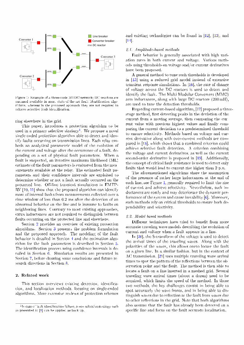
The relative precision of the estimated distance for thedierent fault cases is summarized and compared with sev-eral state-of-the-art methods in the Table 6. The distanceerror is dened as a percentage of the total length of the

line, ed =(df − d∗f

)/d. Though the precision of the pro-

posed approach is lower, it is able to take the decision totrip the line using a measurement window 20 times smaller

Figure 17: Duration of the observation window required for faultidentication at relays R31 and R13.

Figure 18: Relative error of the estimated fault distance at relaysR31 and R13 for the extensive simulation fault cases.

150 160 170 180 190 200 210 220 230

0

20

40

60

80

100

120

140

Figure 19: Results at relay R23: The green area indicates faultsthat were correctly identied as external; The red area correspondsto faults that were incorrectly identied in the protected line L23;Distance corresponds to the total distance between the fault andrelay R23; Case 1 with R∗

f= 20 Ω, d∗

f= 180 km is indicated by a

cross.

than the other methods. This makes it suitable as a pri-mary fault identication algorithm for selective protectionstrategies. For the proposed approach the distribution ofthe error for the dierent fault cases is detailed in Fig-ure 18. The relative error is less than 5% of the total linelength for more 40 cases which represents about half of thefault cases identied on line L13.

The selectivity analysis is presented for the relay R23 inFigure 19. Selectivity at the three other relays is ensuredin all fault cases, due to the direction of the current wavewhich travels backwards. This is not the case for relay R23

and selectivity may be a challenge in some cases. This canbe observed in Figure 12 where the area of the condenceellipse evaluated at R23 goes much closer to the thresholdcompared to that evaluated at relays R21, R12, or R32.The green area corresponds to faults that were correctlyidentied as outside the monitored line L23. The red areacorresponds to faults that were incorrectly identied inline L23. Distances represent the total distance betweenthe faults and relay R23. The algorithm is selective for awide range of fault cases. Few selectivity failures can benoticed for faults occurring very close to the relay R31 andhaving a low impedance. In such cases, the estimationalgorithm wrongly identies the fault in line L23 with alarge fault distance and resistance.

In summary, the simulations show that the proposedapproach has a satisfying behavior over a wide range of

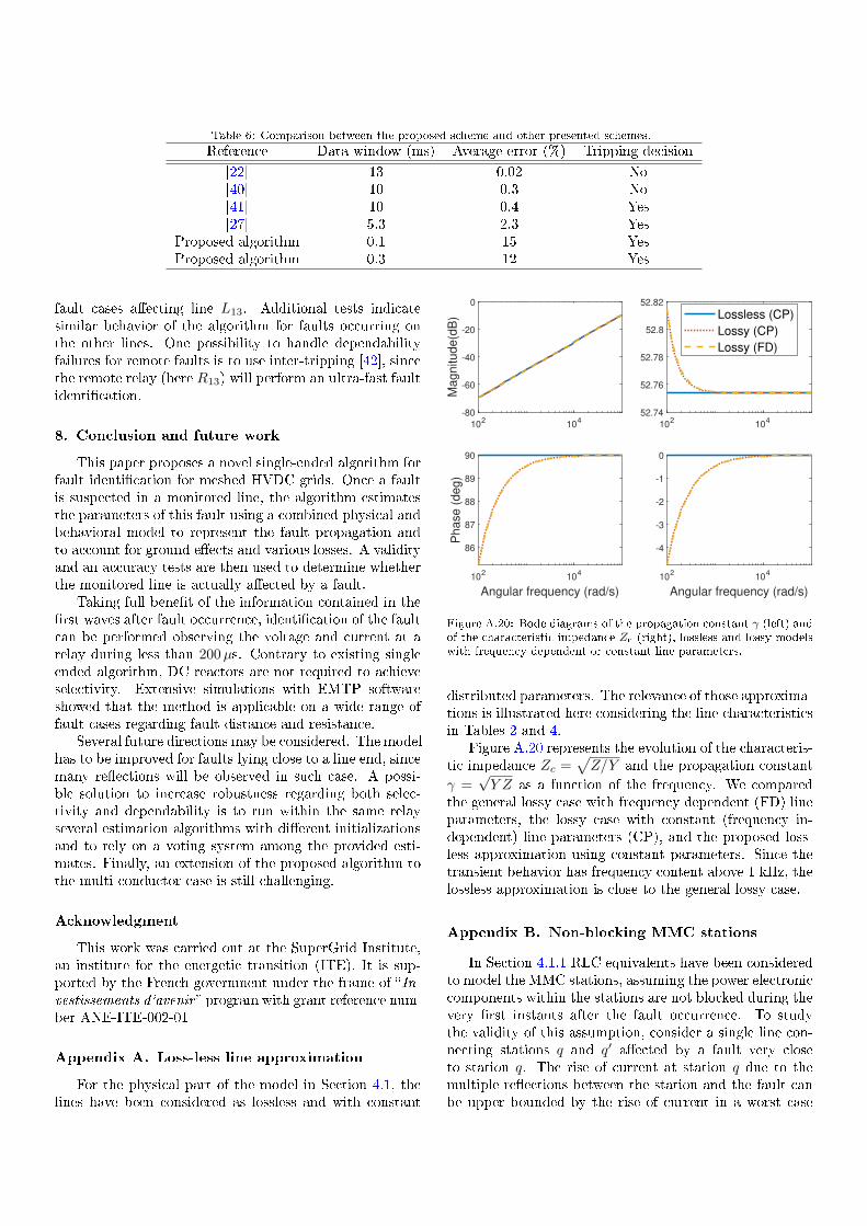
Table 6: Comparison between the proposed scheme and other presented schemes.

Reference Data window (ms) Average error (%) Tripping decision

[22] 13 0.02 No[40] 10 0.3 No[41] 10 0.4 Yes[27] 5.3 2.3 Yes

Proposed algorithm 0.1 15 YesProposed algorithm 0.3 12 Yes

fault cases aecting line L13. Additional tests indicatesimilar behavior of the algorithm for faults occurring onthe other lines. One possibility to handle dependabilityfailures for remote faults is to use inter-tripping [42], sincethe remote relay (here R13) will perform an ultra-fast faultidentication.

8. Conclusion and future work

This paper proposes a novel single-ended algorithm forfault identication for meshed HVDC grids. Once a faultis suspected in a monitored line, the algorithm estimatesthe parameters of this fault using a combined physical andbehavioral model to represent the fault propagation andto account for ground eects and various losses. A validityand an accuracy tests are then used to determine whetherthe monitored line is actually aected by a fault.

Taking full benet of the information contained in therst waves after fault occurrence, identication of the faultcan be performed observing the voltage and current at arelay during less than 200µs. Contrary to existing singleended algorithm, DC reactors are not required to achieveselectivity. Extensive simulations with EMTP softwareshowed that the method is applicable on a wide range offault cases regarding fault distance and resistance.

Several future directions may be considered. The modelhas to be improved for faults lying close to a line end, sincemany reections will be observed in such case. A possi-ble solution to increase robustness regarding both selec-tivity and dependability is to run within the same relayseveral estimation algorithms with dierent initializationsand to rely on a voting system among the provided esti-mates. Finally, an extension of the proposed algorithm tothe multi-conductor case is still challenging.

Acknowledgment

This work was carried out at the SuperGrid Institute,an institute for the energetic transition (ITE). It is sup-ported by the French government under the frame of In-vestissements d'avenir program with grant reference num-ber ANE-ITE-002-01

Appendix A. Loss-less line approximation

For the physical part of the model in Section 4.1, thelines have been considered as lossless and with constant

102

104

-80

-60

-40

-20

0

Ma

gn

itu

de

(dB

)

102

104

52.74

52.76

52.78

52.8

52.82

Lossless (CP)

Lossy (CP)

Lossy (FD)

102

104

Angular frequency (rad/s)

86

87

88

89

90P

ha

se

(d

eg

)

102

104

Angular frequency (rad/s)

-4

-3

-2

-1

0

Figure A.20: Bode diagrams of the propagation constant γ (left) andof the characteristic impedance Zc (right), lossless and lossy modelswith frequency dependent or constant line parameters.

distributed parameters. The relevance of those approxima-tions is illustrated here considering the line characteristicsin Tables 2 and 4.

Figure A.20 represents the evolution of the characteris-tic impedance Zc =

√Z/Y and the propagation constant

γ =√Y Z as a function of the frequency. We compared

the general lossy case with frequency dependent (FD) lineparameters, the lossy case with constant (frequency in-dependent) line parameters (CP), and the proposed loss-less approximation using constant parameters. Since thetransient behavior has frequency content above 1 kHz, thelossless approximation is close to the general lossy case.

Appendix B. Non-blocking MMC stations

In Section 4.1.1 RLC equivalents have been consideredto model the MMC stations, assuming the power electroniccomponents within the stations are not blocked during thevery rst instants after the fault occurrence. To studythe validity of this assumption, consider a single line con-necting stations q and q′ aected by a fault very closeto station q. The rise of current at station q due to themultiple reections between the station and the fault canbe upper bounded by the rise of current in a worst case

scenario, where the fault is an ideal short-circuit and thestation is an ideal voltage source. In that case each trav-eling wave reaching the station q will increase the currentowing through the MMC by a step of magnitude 2 vbfZc .Considering that the prior fault voltage is close to thenominal DC voltage VDC, this step can be converted inper unit using the nominal DC power PDC as,

2V 2DC

ZcPDC.

Thus, the per unit value of the current owing through theMMC after 2 traveling waves is

1 + 4V 2DC

ZcPDC,

again considering a worst case where the prior fault cur-rent in the line is 1p.u. For the parameters considered inSection 7.1 the current reaches 1.94p.u. The auto-blockingof the IGBTs within the MMC is generally considered tobe active when the current reaches 2p.u. Hence, consider-ing that the previous derivations are rather conservative,it is reasonable to model the 2 rst waves assuming theMMC are not blocked.

References

[1] E. Pierri, O. Binder, N. G. Hemdan, M. Kurrat, Challengesand opportunities for a European HVDC grid, Renewable andSustainable Energy Reviews 70 (2017) 427456. doi:10.1016/

j.rser.2016.11.233.[2] P. Rodriguez, K. Rouzbehi, Multi-terminal DC grids: challenges

and prospects, Journal of Modern Power Systems and Clean En-ergy 5 (4) (2017) 515523. doi:10.1007/s40565-017-0305-0.

[3] WP4 PROMOTIoN, Report on the broad comparison of pro-tection philosophies for the identied grid topologies, Tech. rep.(2018).

[4] CIGRE B4/B5.59, Protection and local control of HVDC-grids,Tech. rep., CIGRE (2018).

[5] D. Van Hertem, O. Gomis-Bellmunt, J. Liang, HVDC Grids ForOshore and Supergrid of the Future, Wiley-IEEE Press, 2016.

[6] K. Shinoda, A. Benchaib, J. Dai, X. Guillaud, Virtual CapacitorControl for Stability Improvement of HVDC System Compris-ing DC Reactors, in: Proc. Conference on AC and DC PowerTransmission, 2019, pp. 16.

[7] WP6 PROMOTIoN, Develop system level model for hybrid DCCB, Tech. Rep. 691714 (2016).

[8] N. Johannesson, S. Norrga, Estimation of travelling wave arrivaltime in longitudinal dierential protections for multi-terminalHVDC systems, Proc. 14th International Conference on Devel-opments in Power System Protection (DPSP 2018) 2018 (15)(2018) 10071011. doi:10.1049/joe.2018.0225.

[9] D. Loume, A. Bertinato, B. Raison, B. Luscan, A multi-vendorprotection strategy for HVDC grids based on low-speed DC cir-cuit breakers, in: Proc. 13th IET International Conference onAC and DC Power Transmission (ACDC), Manchester, 2017,pp. 16. doi:10.1049/cp.2017.0008.

[10] Hermann W. Dommel, Digital Computer Solution of Electro-magnetic Transients in Single-and Multiphase Networks, IEEETransactions on Power Apparatus and Systems 88 (4) (1969)388 399. doi:10.1109/TPAS.1969.292459.

[11] J. Mahseredjian, S. Dennetière, L. Dubé, B. Khodabakhchian,L. Gérin-Lajoie, On a new approach for the simulation oftransients in power systems, Electric Power Systems Research77 (11) (2007) 15141520.

[12] S. Le Blond, R. Bertho, D. V. Coury, J. C. Vieira, Designof protection schemes for multi-terminal HVDC systems, Re-newable and Sustainable Energy Reviews 56 (2016) 965974.doi:10.1016/j.rser.2015.12.025.

[13] B. Chang, O. Cwikowski, M. Barnes, R. Shuttleworth, A. Bed-dard, P. Coventry, Review of dierent fault detection meth-ods and their impact on pre-emptive VSC-HVDC dc protec-tion performance, High Voltage 2 (4) (2017) 211219. doi:

10.1049/hve.2017.0024.[14] M. Ashouri, C. L. Bak, F. Faria Da Silva, A review of the

protection algorithms for multi-terminal VCD-HVDC grids, in:Proc. IEEE International Conference on Industrial Technology(ICIT), 2018, pp. 16731678. doi:10.1109/ICIT.2018.8352433.

[15] W. Leterme, J. Beerten, D. Van Hertem, Non-unit protec-tion of HVDC grids with inductive DC cable termination,IEEE Transactions on Power Delivery 31 (2) (2016) 820828.doi:10.1109/TPWRD.2015.2422145.

[16] R. Li, L. Xu, L. Yao, DC fault detection and location in meshedmultiterminal HVDC systems based on DC reactor voltagechange rate, IEEE Transactions on Power Delivery 32 (3) (2017)15161526. doi:10.1109/TPWRD.2016.2590501.

[17] S. Pirooz Azad, D. Van Hertem, A Fast Local Bus Current-Based Primary Relaying Algorithm for HVDC Grids, IEEETransactions on Power Delivery 32 (1) (2017) 193202. doi:

10.1109/TPWRD.2016.2595323.[18] A.-K. Marten, C. Troitzsch, D. Westermann, Non-

telecommunication based DC line fault detection method-ology for meshed HVDC grids, in: Proc. AC andDC Power Transmission (ACDC), Birmingham, 2015.doi:10.1049/iet-gtd.2015.0700.

[19] G. Auran, J. Descloux, S. Nguefeu, B. Raison, Non-unit fullselective protection algorithm for MTDC grids, in: Proc. IEEEPower & Energy Society General Meeting, Chicago, 2017, pp.15.

[20] C. Xi, Q. Chen, L. Wang, A single-terminal traveling wave faultlocation method for VSC-HVDC transmission lines based onS-transform, in: Proc. IEEE PES Asia-Pacic Power and En-ergy Engineering Conference (APPEEC), Xi'an, 2016, pp. 10081012. doi:10.1109/APPEEC.2016.7779647.

[21] A. Guzman-Casillas, B. Kasztenny, Y. Tong, M. V. Mynam, Ac-curate single-end fault locating using traveling-wave reectioninformation, in: Proc. Developments In Power System Protec-tion, Belfast, 2018, pp. 16.

[22] J. Suonan, S. Gao, G. Song, Z. Jiao, X. Kang, A novel fault-location method for HVDC transmission lines, IEEE Trans-actions on Power Delivery 25 (2) (2010) 12031209. doi:

10.1109/TPWRD.2009.2033078.[23] Y. Liu, A. Sakis Meliopoulos, Z. Tan, L. Sun, R. Fan, Dynamic

state estimation-based fault locating on transmission lines, IETGeneration, Transmission & Distribution 11 (17) (2017) 41844192. doi:10.1049/iet-gtd.2017.0371.

[24] R. Razzaghi, G. Lugrin, H. Manesh, C. Romero, M. Paolone,F. Rachidi, An ecient method based on the electromagnetictime reversal to locate faults in power networks, IEEE Trans-actions on Power Delivery 28 (3) (2013) 16631673. doi:

10.1109/TPWRD.2013.2251911.[25] X. Jin, G. Song, Z. Ma, A Novel Pilot Protection for VSC-

HVDC Transmission Lines Based on Parameter Identication,in: Proc. 12th IET International Conference on Developmentsin Power System Protection (DPSP), Vol. 05, Institution of En-gineering and Technology, Copenhagen, 2014, pp. 16. doi:

10.4236/epe.2013.54B224.[26] N. Johannesson, S. Norrga, C. Wikström, Selective Wave-Front

Based Protection Algorithm for MTDC Systems, in: Proc. 13thInternational Conference on Development in Power System Pro-tection (DPSP), Edinburgh, 2016, pp. 16. doi:10.1049/cp.

2016.0051.

[27] A. Ali Al Hage, B. Piepenbreier, D. Buchstaller, M. Engel,Multiple model based fault localization for HVDC transmis-sion systems: Robustness and real-world performance, in: Proc.IEEE/PES Transmission and Distribution Conference and Ex-position (T&D), Dallas, 2016, pp. 15. doi:10.1109/TDC.2016.7519987.

[28] M. Wang, J. Beerten, D. Van Hertem, Frequency domain basedDC fault analysis for bipolar HVDC grids, Journal of ModernPower Systems and Clean Energy 5 (4) (2017) 548559. doi:

10.1007/s40565-017-0307-y.[29] L. Bewley, Traveling Waves on Transmission Systems, Transac-

tions of the American Institute of Electrical Engineers 50 (2)(1931) 532550. doi:10.1109/ee.1942.6436308.

[30] G. Auran, Full selective protection strategy for multi-terminalcable HVDC grids based on HB-MMC converters, Phd the-sis, Université Grenoble Alpes (2017). doi:10.1097/JGP.

0b013e31819e2d50.[31] W. Leterme, D. Van Hertem, Reduced Modular Multilevel

Converter Model to Evaluate Fault Transients in DC Grids,in: Proc. 12th IET International Conference on Developmentsin Power System Protection (DPSP), 2014. doi:10.1049/cp.

2014.0107.[32] J. De Andrade Suárez, E. Sorrentino, Typical expected values

of the fault resistance in power systems, in: Proc. IEEE/PESTransmission and Distribution Conference and Exposition:Latin America, Sao Paulo, 2010, pp. 602609. doi:10.1109/

TDC-LA.2010.5762944.[33] A. Wasserrab, G. Balzer, The signicance of frequency-

dependent overhead lines for the calculation of HVDC lineshort-circuit currents, Electrical Engineering 97 (3) (2015) 213223. doi:10.1007/s00202-014-0323-0.

[34] L. Ljung, System Identication - Theory for the User, Prentice-Hall, Englewood Clis, NJ, 1987.

[35] E. Walter, L. Pronzato, Identication of parametric models fromexperimental data, Springer-Verlag London, 1997.

[36] S. M. Kay, Fundamentals of Statistical Signal Processing: Esti-mation Theory, Prentice Hall PTR, 1993.

[37] A. Zama, S. Bacha, A. Benchaib, D. Frey, S. Silvant, A novelmodular multilevel converter modelling technique based onsemi-analytical models for HVDC application, Journal of Elec-trical Systems 12 (4) (2016) 649659.

[38] O. R. Leanos, Wideband Line Cable Models for Realt Time andO Line Simulations of ElectroMagnetic Transients, Phd thesis,Ecole Polytechnique de Montréal (2013).

[39] IEEE Substations Committee, IEEE Guide for Measuring EarthResistivity, Ground Impedance, and Earth Surface Potentials ofa Grounding System - Redline, Tech. rep. (2012). doi:10.1109/IEEESTD.2012.6392181.

[40] M. Farshad, J. Sadeh, A novel fault-location method for HVDCtransmission lines based on similarity measure of voltage signals,IEEE Transactions on Power Delivery 28 (4) (2013) 24832490.doi:10.1109/TPWRD.2013.2272436.

[41] A. E. Abu-Elanien, A. A. Elserougi, A. S. Abdel-Khalik, A. M.Massoud, S. Ahmed, A dierential protection technique formulti-terminal HVDC, Electric Power Systems Research 130(2016) 7888. doi:10.1016/j.epsr.2015.08.021.URL http://dx.doi.org/10.1016/j.epsr.2015.08.021

[42] Network Protection & Automation Guide, Alstom Grid, 2011.