Network Competition in the Airline Industry: A Framework ...
67
Electronic copy available at: https://ssrn.com/abstract=3246222 Network Competition in the Airline Industry: A Framework for Empirical Policy Analysis * Zhe Yuan † September 8, 2018 * I am grateful to Victor Aguirregabiria for his supervision and continuous encouragement, as well as to thank my committee members, Andrew Ching, Mara Lederman, and Yao Luo, for their support and feedback. I would also like to thank Loren Brandt, Heski Bar-Isaac, Dwayne Ben- jamin, Rahul Deb, Gerard Llobet, Robert McMillan, Matthew Mitchell, Xiao Mo, Ismael Mourifi´ e, Salvador Navarro, Rob Porter, James Roberts, Eduardo Souza-Rodrigues, Xianwen Shi, Junichi Suzuki, Yuanyuan Wan, Daniel Xu, and seminar participants at Albany, Ryerson, Saskatchewan, Toronto, Western, Renmin University, CEA Annual Conference 2016, IIOC Annual Conference 2016, SHUFE IO Conference, 2nd International Conference on Network Economics and Big Data, EARIE Annual Conference 2016, and China Meeting for Econometric Society 2017, for helpful comments and discussion. All errors are my own. † Alibaba Group, 969 Wenyi West Road, Hangzhou, Zhejiang, China 200433.[email protected]. 1
Transcript of Network Competition in the Airline Industry: A Framework ...

Electronic copy available at: https://ssrn.com/abstract=3246222
Network Competition in the Airline Industry:
A Framework for Empirical Policy Analysis∗
Zhe Yuan†
September 8, 2018
∗I am grateful to Victor Aguirregabiria for his supervision and continuous encouragement, as
well as to thank my committee members, Andrew Ching, Mara Lederman, and Yao Luo, for their
support and feedback. I would also like to thank Loren Brandt, Heski Bar-Isaac, Dwayne Ben-
jamin, Rahul Deb, Gerard Llobet, Robert McMillan, Matthew Mitchell, Xiao Mo, Ismael Mourifie,
Salvador Navarro, Rob Porter, James Roberts, Eduardo Souza-Rodrigues, Xianwen Shi, Junichi
Suzuki, Yuanyuan Wan, Daniel Xu, and seminar participants at Albany, Ryerson, Saskatchewan,
Toronto, Western, Renmin University, CEA Annual Conference 2016, IIOC Annual Conference 2016,
SHUFE IO Conference, 2nd International Conference on Network Economics and Big Data, EARIE
Annual Conference 2016, and China Meeting for Econometric Society 2017, for helpful comments
and discussion. All errors are my own.†Alibaba Group, 969 Wenyi West Road, Hangzhou, Zhejiang, China
1

Electronic copy available at: https://ssrn.com/abstract=3246222
Abstract
This paper studies network competition in the U.S. airline industry and pro-
pose a structural model of oligopoly competition where the set of endogenous
strategic decisions of an airline includes its network structure (i.e., the set of
city-pair markets where the airline operates nonstop flights), flight frequency
(the number of daily flights) for every market in which the airline is active, and
pricing for all nonstop and one-stop services. Furthermore, this paper proposes
a simple methodology for both model estimation and counterfactual experi-
ment evaluation that avoids the computation of a network equilibrium. The
estimated model demonstrates that ignoring endogenous network structure in
this industry implies a substantial (11 percent) downward bias on estimates of
the marginal variable profits and marginal costs of scheduling flight frequency.
Applying the estimated model to evaluate the consequences of a hypotheti-
cal merger between Alaska Airlines and Virgin America in the first quarter of
2014 shows that the hypothetical post-merger airline would re-optimize its net-
work structure, entering 32 nonstop markets and exiting 13 nonstop markets.
Though overall consumer surplus increases post-merger, there is heterogeneity
in consumer surplus change across markets in that consumer surplus increases
in larger markets but slightly decreases in smaller markets.
Key words: Airline industry, Entry models, Network competition, Moment
inequalities, Counterfactual experiments
JEL: C30 C51 C72 L13 L14 L93
This version: September 8, 2018
1 Introduction
The U.S. airline industry helps drive nearly $1.5 trillion in U.S. economic activity
(almost 10% of U.S. GDP) and is relevant to more than 11 million jobs. One of the
most important strategic choices for an airline is deciding the markets in which to
2

Electronic copy available at: https://ssrn.com/abstract=3246222
operate direct flights.1 This entry decision determines the network structure of the
airline, or specifically, the set of markets that the airline serves and whether these
markets are served with direct flights or flights with connections. There are substan-
tial interdependence and synergies between an airline’s entry decisions into different
markets. Some of these synergies have to do with economies of scale and scope at the
airline-airport level, e.g., the additional cost of operating flights between cities A and
B could be lower if the airline already operates in other markets in addition to A or B.
However, the most obvious interdependence between the entry decisions for different
markets is that they determine the set of markets with connections (or stops) that the
airline operates. For instance, suppose an airline operates direct flights between cities
A and B, and is deciding whether to start operating flights either between cities B
and C or between C and D. Supposing that the operating costs and demand of these
new markets are similar, one would expect this airline to choose to operate between
cities B and C rather than between C and D simply because the first choice would
also attract new passengers travelling between A and C with a stop in city B.
This paper wants to answer two research questions related to airline networks:
first, how do airlines’ entry, exit and flight frequency decisions depend on the network
structure, or specifically, the market structures in the other parts of the network.
Second, if two airlines merge into a new airline, how does this post-merger airline
optimize its network structure. The network of the post-merger airline is not a simple
combination of the two pre-merger networks. There may be entries, exits or flight
frequency re-allocations in many markets, even in markets where airlines are not
active before.
Structural papers studying the airline industry, pioneered by Berry (1992), have
answered important questions related to airline demand, cost structure, strategic in-
teractions, and entry deterrence.2 However, most models of entry in this literature
1A market is a non-directional city pair in which airlines transport passengers from wither cityto the other city.
2The growing literature includes Berry (1990), Berry (1992), Brueckner and Spiller (1994), Berry,Carnall, and Spiller (2006), Williams (2008), Ciliberto and Tamer (2009), Snider (2009), Berry and
3

Electronic copy available at: https://ssrn.com/abstract=3246222
have ignored or simplified the interconnectionness of markets and treated airline net-
works as exogenously given, often making the assumption that the airline entry, exit,
and flight frequency decisions in one market is independent to its structure across
markets. This would make sense if there were no synergies across markets, since
airlines would make entry and flight frequency decisions based on local market char-
acteristics without considering overall market network structure. However, network
structure is the key feature of this industry. For example, suppose two airlines merge
into a new airline. The optimal network of the post-merger airline would not merely
be a combination of the two pre-merger networks but a much larger network with
a potential re-allocation of flight frequencies across its network and/or entry into
new markets. Without a model endogenizing the network structure of the airlines, it
would not be possible to study can not answer the research questions of this paper.
To answer these questions, I develop a three-stage model of airline network com-
petition, modelling airline competition as a static game of complete information in
which network structure, flight frequency, and price for every nonstop and one-stop
market are endogenized. In the first (entry) stage, airlines choose their network struc-
ture, i.e., the set of markets in which they operate nonstop flights, which determines
the set of nonstop and one-stop products available to consumers. In the second (flight
frequency) stage, airlines decide their flight frequency for every nonstop market, which
determines the total number of nonstop and one-stop service offerings in all markets.
In the third stage, airlines compete with respect to prices in every market given their
network structure and flight frequencies. Consumers decide which airline service to
purchase after observing the prices and quality of all products. Airlines earn variable
profits from both nonstop and one-stop products.
It is computationally challenging to estimate a three-stage network competition
model. The number of strategies or networks of an airline increases exponentially
Jia (2010), Aguirregabiria and Ho (2012), Ciliberto and Williams (2014), Ciliberto and Zhang (2014),Gedge, Roberts, and Sweeting (2017), Kundu (2014), Onishi and Omori (2014), Blevins (2015) andGayle and Yimga (2015).
4

Electronic copy available at: https://ssrn.com/abstract=3246222
with the number of markets in the network and estimating the complete information
game usually requires computing for an equilibrium of the model (Berry, 1992) or
solving for the upper and lower bounds of choice probabilities (Ciliberto and Tamer,
2009).3 For network competition games, computation of an equilibrium is infeasible
even for a simple entry game with only a small number of players. While Jia (2008)
makes use of the supermodularity of the game to compute Nash equilibria for net-
work competition games with two players. Her method, nonetheless, doesn’t apply to
the US airline industry where there are more than two major players. Furthermore,
estimation of incomplete information games usually requires estimating conditional
choice probabilities, which is impossible with high-dimensional strategy space. The
existing literature proposes various assumptions to reduce the dimensionality of strat-
egy space. For example, Aguirregabiria and Ho (2012) assume that every airline has
a local manager in every market who decides whether the airline will enter or exit the
local markets independently, which substantially reduces the dimensionality of the
strategy space.
As an alternative, the current paper proposes and implements a simple methodol-
ogy for model estimation and the evaluation of counterfactual experiments that does
not require solving for a network equilibrium. First, I estimate the demand systems
and back out the marginal costs of serving passengers. Both consumer utility and
airline marginal cost of serving passengers depend on airline flight frequency. Next, I
estimate the cost structure of airlines associated with network structure. Assuming
that the network structures observed in the data are those of Nash equilibrium, I esti-
mate airline’ cost of scheduling flight frequencies using the flight frequency marginal
condition of optimality. In other words, an airline that is active in a market will
schedule flights in this market until the marginal variable profit (MVP) of an ad-
ditional flight equals the marginal cost (MC) of scheduling this flight. Specifically,
the MVP of an additional flight is the sum of the following four components: (a) a
3In a world with 87 cities, the number of possible strategy profiles would be 287×86/2 ' 1.4×101126
and the number of feasible network configurations with 13 airlines would be 213×87×86/2 ' 1014640.
5

Electronic copy available at: https://ssrn.com/abstract=3246222
MVP from additional nonstop service, (b) a MVP from additional one-stop services,
(c) a cannibalization effect from additional nonstop service and (d) a cannibalization
effect from additional one-stop services. Finally, I estimate entry costs by exploiting
the inequality restrictions implied by airline best response conditions in the entry
game. If an airline operates direct service in a market, its entry cost is lower than its
counterfactual variable profit if it exits this market. This generates an upper bound
for entry cost. If an airline does not operate direct service in a market, its entry
cost is higher than its counterfactual variable profit if it enters this market with op-
timal flight frequency. This generates a lower bound for entry cost. These two model
restrictions minimize violations of entry cost estimates.
In a counterfactual experiment, I investigate the network structure after an ex-
ogenous hypothetical merger between Alaska Airline and Virgin America. Since it
is computationally infeasible to obtain a Nash equilibrium of this simultaneous-move
network competition game, I reconstruct this simultaneous game as a sequential-move
game. I start by proposing a sequence by which all airline-market pairs move. Air-
lines first move in larger markets followed by smaller markets. Within each market,
airlines move sequentially by profitability. In this way, I obtain the order by which all
airline-market pairs move in this massive sequential move game. While it would be
ideal to solve for the sub-game perfect Nash equilibrium using backward induction,
it is impossible to compute airline profits at all branches of the game tree, so I use
a forward-induction algorithm to search for an equilibrium. Starting with an empty
network where no airlines are active in any market, I repetitive airline best response,
airline-market pair by airline-market pair according to the sequence defined above.
Specifically, starting with the most profitable airline in the largest market, I deter-
mine the optimal action of this airline in that specific market. I update the airline’s
network structure each time it enters, exits, or changes flight frequency in a market.
Then, I proceed to the second most profitable airline in the largest market, evaluate
the best response of this airline in the market and update its network structure, and
6

Electronic copy available at: https://ssrn.com/abstract=3246222
so on. After visiting all airline-market pairs, I return to the first airline-market pair
and re-evaluate the best responses of the entire airline-market sequence. If there is
no incentive to deviate, this convergence of best responses in the network serves as an
approximation of the subgame perfect Nash equilibrium of the sequential-move game.
The empirical finding shows that, on average, marginal variable cost and marginal
variable profit from scheduling an additional flight is $7553. However, if endogenous
network structures are ignored, these values would be underestimated by 13%. The
counterfactual experiment shows that, if Alaska Airline and Virgin America merge in
the first quarter of 2014, the new post-merger airline will enter 32 nonstop markets
and exit 13 nonstop markets. Though overall consumer surplus increases post-merger,
there is heterogeneity in consumer surplus change across markets in that consumer
surplus will increase in larger markets but slightly decrease in smaller markets.
There are four main contributions in this paper. First, I construct and esti-
mate an equilibrium model of network competition, endogenizing network structures,
product quality (flight frequencies), price and number of consumers for every non-
stop and one-stop market and estimating consumer demand together with endoge-
nous product characteristics (flight frequencies) and endogenous network structures
(entry decisions). Second, this paper implements a moment inequality method to
obtain a consistent estimator of entry cost under mild conditions. The empirical
framework is based upon the necessary conditions of pure strategy Nash equilibrium,
which avoids the solution of the model and is computationally feasible. I extend and
implement a swapping method in the spirit of Pakes, Porter, Ho, and Ishii (2015)
and Ellickson, Houghton, and Timmins (2013), and the bound estimator proposed
in Aguirregabiria, Clark, and Wang (2016), and obtain consistent estimates of fixed
cost under mild conditions. Third, I propose a novel algorithm to investigate the
consequences of an exogenous merger between two airlines. This algorithm allows
me to compare the change in network structures and consumer welfare pre-merger
and post-merger. Fourth, I propose measures of flight frequency for both nonstop
7

Electronic copy available at: https://ssrn.com/abstract=3246222
and one-stop services, which are measures of product quality and incorporated as
important endogenous choices of the airlines.
This paper also makes important contributions to the research on network com-
petition. First, this paper studies a new type of network synergy — economies of
scope. Suppose an airline operates direct flights in market AB, its entry into market
BC generates two new products to consumers: nonstop service in market BC and
one-stop service in market AC with a stop at city B. In contrast, existing models
on network competition focus on economies of scale: a firm has a lower cost if it
operates many stores in this market. Second, this paper allows for rich heterogeneity
in synergy between any two markets. In the airline industry, synergy between two
markets is the profitability of the one-stop service through the two markets. This
synergy depends on not only the number of direct flights in these two markets but
also technology determinifng the feasibility and efficiency of the connecting service.
I use two matrices to represent the network structures of an airline: one matrix for
nonstop service and another matrix for one-stop service. As a comparison, other
papers measure synergy by the distance between two stores (Jia, 2008), the number
of airline routes connected to a city (Aguirregabiria and Ho, 2012), or the number of
stores in a market (Ellickson, Houghton, and Timmins, 2013). Third, this paper ex-
plicitly models consumer utility and airline product quality decisions, both of which
are abstracted in other models of network competition. Lastly, I propose an algo-
rithm to compute a network equilibrium such that I can compare the airline networks
pre-merger and post-merger.
This paper builds on and contributes to three streams of literature. In terms of
research on the airline industry, previous studies have discussed the benefits of air-
line hubs, including cost efficiency (Berry, 1990, 1992; Brueckner and Spiller, 1994;
Berry, Carnall, and Spiller, 2006; Ciliberto and Tamer, 2009), demand factors (Berry,
1990; Berry and Jia, 2010), and strategic entry deterrence (Hendricks, Piccione, and
Tan, 1997, 1999; Aguirregabiria and Ho, 2012). Few structural models of entry in
8
Electronic copy available at: https://ssrn.com/abstract=3246222
the airline industry study synergies between an airline entry decisions in different
markets. Aguirregabiria and Ho (2012) is the first paper to empirically estimate a
network competition game with exogenous network structure. Dou, Lazarev, and
Kastl (2017) study the externalities of airline delays throughout airline networks.
There are rich studies on the pricing strategies of the airlines. Williams (2008) esti-
mates a dynamic equilibrium model where firms first invest in seating capacity and
then play a capacity-constrained pricing game. Lazarev (2013) studies intertempo-
ral price discrimination on monopoly routes in the airline industry and evaluate its
welfare consequences. Williams (2017) separately studies both intertemporal price
discrimination and dynamic adjustment to stochastic demand. Gedge, Roberts, and
Sweeting (2017) propose a model of limited pricing to explain that incumbent prices
are lower when Southwest becomes a potential entrant.
This paper also relates to research on the estimation of entry games with network
competition. Most entry models ignore interconnections across markets with several
exceptions: Seim (2006) studies spatial competition in the video rental industry. Her
model endogenizes store locations and estimates an entry game of spatial competition.
Zhu and Singh (2009) employ a more flexible model of spatial competition and allow
for more general heterogeneity across firms. Jia (2008) analyzes the network entry
game between Wal-Mart and Kmart over 2065 locations. She considers a specification
of the profit function which implies the supermodularity of the game and facilitates the
computation of an equilibrium. While her model allows for the economies of density,
it ignores cannibalization effects and spatial competition between stores of different
chains at different locations. Nishida (2014) extends Jia’s model by allowing for
multiple stores in the same location and incorporates spatial competition. Ellickson,
Houghton, and Timmins (2013) and Aguirregabiria, Clark, and Wang (2016) estimate
network economics in retail chains and the banking industry, respectively.
Lastly, this paper contributes to research on airline mergers. Richard (2003) finds
that mergers are associated with increased flight frequencies and that the overall effect
9

Electronic copy available at: https://ssrn.com/abstract=3246222
of mergers on welfare varies by markets. Peters (2006) uses merger simulations to
predict post-merger prices for six major airline mergers from the 1980’s, and compares
these predictions with actual post-merger prices. Ciliberto, Murry, and Tamer (2016)
and Li, Mazur, Park, Roberts, Sweeting, and Zhang (2018) study endogenous market
entry with post-merger selection. Ciliberto, Cook, and Williams (2018) use measures
of centrality from graph theory to study the effect of consolidation on airline network
connectivity. There is also an extensive literature on mergers in other industries. For
instance, Nevo (2000) studies how prices and consumer welfare change after a merger
in the ready-to-eat cereal industry. Fan (2013) allows for changes in both prices
and product characteristics after ownership consolidation. Most research on mergers
study within market mergers but few papers study mergers between two networks.
The closest research to this paper is Benkard, Bodoh-Creed, and Lazarev (2010),
which estimates dynamic changes in the airline industry after mergers. Their merger
analysis is based on simulation of policy functions (choice probabilities) and assume
that firms’ strategy functions do not change pre-merger and post-merger. Though
my model is static, it is based on profit maximization behaviors of players and has a
clear equilibrium concept.
The remainders of the paper are organized as follows. Section 2 a model of airline
competition. Section 3 describes the data and construction of the working sample.
Section 4 presents the assumptions and empirical strategy. Section 5 presents the em-
pirical results. Section 6 discusses the counterfactual analysis. Section 7 summarizes
and concludes.
2 Model
The model is a game of network competition, as in the models of competition between
retail networks in Jia (2008), Ellickson, Houghton, and Timmins (2013), and Aguirre-
10
Electronic copy available at: https://ssrn.com/abstract=3246222
gabiria, Clark, and Wang (2016).4 However, the game of competition between airline
networks has some important distinguishing features with respect to existing models
of retail networks. Network synergies in retail industries are about economies of scale
or density at the local market level: firms receive higher profit if they have more
stores in a market. In contrast, network synergy in the airline industry is about eco-
nomics of scope: if an airline operates two direct flights, it may operate an additional
one-stop flight which introduces an important interconnection between airlines’ entry
and flight frequency decisions in different markets. While most existing literature
treats airline network structures as exogenous, I construct a game of airline network
competition that endogenizes the network structure of the airlines.
2.1 Notation and Timeline
The industry is configured by N airlines (indexed by n) and C cities. From the point
of view of airline operation and competition, a market is a non-directional city-pair
in which airlines provide regular commercial aviation service. In a world with C
cities, there are M = C×(C−1)2
markets.5 Markets are indexed by ij, with i and j
representing the two endpoint cities. Airlines can provide both nonstop and one-stop
services in this market.
Airline n can provide at most two different types of services (or two products) in
a market ij. Service in market ij without a stop is referred to as nonstop service
and service between i and j with a stop in a third city is referred to as one-stop
4I consider a static model rather than a dynamic model. If the profit function in the static gameis treated as present value of the dynamic game under the assumption that there will not be changesin the network and the adjustment cost function, the static game is equivalent to a dynamic game.My paper is not the only paper that models a complicated dynamic game as a static game. Otherpapers include Jia (2008) and Ellickson, Houghton, and Timmins (2013) and Aguirregabiria, Clark,and Wang (2016).
5I follow the approach of Berry (1992) and define markets as city-pairs instead of airport pairs.Berry, Carnall, and Spiller (2006) and Aguirregabiria and Ho (2012) also define markets as city-pairs. Borenstein (1989) and Ciliberto and Tamer (2009) define markets as airport pairs. Theimplicit assumption is that airports in the same city are perfect substitutes in both demand andsupply. This paper ignores competition between airports.
11

Electronic copy available at: https://ssrn.com/abstract=3246222
service.6 Airlines usually connect passengers in their hub cities. For instance, if a
passenger travels from New York to San Francisco, she may take a connection in
Chicago or Atlanta. To simplify the model, I do not distinguish amongst one-stop
services with different connecting cities, but aggregate all possible one-stop services
in market ij into one product and refer to it as one-stop service in market ij. The
network structure of an airline consists of both nonstop and one-stop services in all
markets. The product of an airline includes its nonstop and one-stop services in all
markets.
In every market ij, airline n’s cost structure includes its entry cost (FCnij), vari-
able cost of flight frequency (V Cfnij), variable cost of serving nonstop passengers
(V CNSQnij ), and variable cost of serving one-stop passengers (V COSQ
nij ). Airlines com-
pete in three stages: In the first stage, airlines simultaneously determine their network
structures, or specifically, the set of markets in which to operate direct flights (entry
decisions anij). In the second stage, airlines decide their flight frequencies for every
market in which they are active (flight frequencies fNSnij and fOSnij ). In the third stage,
airlines compete in prices (pNSnij and pOSnij) in all markets given their network structures
and flight frequency allocations, both of which are determined in the first two stages.
The model assumes that consumers choose products that maximize their utility
given individual and product characteristics. Airlines are assumed to maximize their
profits in a three-stage competition with simultaneous moves in each stage.
2.2 Three-stage Model of Airline Competition
This subsection discusses the details of the three-stage model of airline network com-
petition.7
6My analysis is restricted to nonstop and one-stop services but ignore services with more thanone-stop because services with two or more stops comprise of less than 3% of air travel. However, themodel and estimation method can be extended to accommodate services with more than one-stop.
7Alternatively, first stage and second stage may be aggregated into a single stage wherein airlineschoose flight frequency, and zero flight frequency refers to staying out. However, the current three-stage model has several advantages. The first stage and second stages represent the extensive andintensive margins, respectively. Though I could describe these decisions in a single stage, it is
12

Electronic copy available at: https://ssrn.com/abstract=3246222
2.2.1 Firm Behavior: First Stage (Network Stage)
In the first stage, aka the entry or network stage, every airline simultaneously decides
whether or not to operate direct (nonstop) flights in all M markets. This determines
the network structures of the airlines.
Entry Decision
Let anij = 1 if airline n enters market ij, and anij = 0 otherwise. The entry decision
of airline n is measured by a C × C symmetric matrix An where anij is the (i, j)-th
element of An. Airline n can provide one-stop service between city-pair ij with a
connection in k if it operates direct flights in both market ik and market kj (i.e.:
anik = 1 and ankj = 1).
Entry Cost
The total entry cost of airline n sums up the airline’s fixed cost in all markets:
FCn(An) =1
2
∑i
∑j 6=i
FCnij × 1 [anij = 1] , (1)
where FCnij denotes airline n’s entry cost into market ij.
2.2.2 Firm Behavior: Second Stage (Flight Frequency Stage)
In the second stage, airlines determine their flight schedules, or specifically, the types
of aircrafts and time of departure and arrival for their flights in all markets. This
determines the set of nonstop and one-stop products of airlines as well as product
quality.
convenient to describe the model and methods to separate the extensive and intensive margins intwo stages.
13

Electronic copy available at: https://ssrn.com/abstract=3246222
Flight Frequencies
I distinguish between two products and two corresponding flight frequency variables.
If airline n operates fNSnij direct flights in market ij, it provides a nonstop product
to consumers with quality b(fNSnij ). Alternatively, if airline n operates fOSnij one-stop
flights in market ij, it provides a one-stop product to consumers with quality b(fOSnij ).
These flight frequencies measure heterogeneity in airline nonstop and one-stop services
and are important determinants of product quality.
Airline n’s nonstop flight frequency in market ij (fNSnij ) is the number of direct
flights it operates in market ij. I ignore heterogeneity in aircraft type and departure
(arrival) time of flights. The concept of one-stop flight frequency is more subtle.
Airline n’s one-stop flight frequency in market ij with a stop at city k (fOS(k)nij ) is the
number of possible one-stop flights airline n provides between city i and city j with
a connection in city k. One-stop flight frequency depends not only on the number
of flights but also on their departure and arrival schedules such that connections are
feasible. I assume airlines can connect one-stop passengers only in hub cities.8 The
set of hubs of airline n is denoted by Hn. Thus, airline n’s one-stop flight frequency
in market ij sums up its one-stop flight frequencies in all markets with a connection
at all hub cities,
fOSnij =∑k∈Hn
fOS(k)nij . (2)
The details of measuring one-stop flight frequencies and selecting hub cities are de-
scribed in Section 3.4.
Nonstop and one-stop flight frequencies of airline n are measured by two C × C
symmetric matrices FNSn and FOS
n where their (i, j)-th elements are fNSnij and fOSnij , re-
spectively. Let Fn ={FNSn ,FOS
n
}denote airline n’s flight frequencies in the network,
let F−n = {Fn′ , n′ 6= n} denote the flight frequencies of other airlines in the entire
8More than 90% of the connections occur in hub cities.
14

Electronic copy available at: https://ssrn.com/abstract=3246222
network, and let f−nij ={fNS−nij, f
OS−nij
}denote flight frequencies of other airlines in
market ij.
Technological Relationship between Nonstop/One-stop Flight Frequencies
As discussed in the previous subsection, airline n’s one-stop flight frequency between
i and j with a connection in k (fOS(k)nij ) depends on the flight schedules of its two legs:
fNSnik and fNSnkj . For the sake of simplicity, I assume fOS(k)nij is a symmetric function of
fNSnik and fNSnkj :
fOS(k)nij = Λ
(k)nij
(fNSnik , f
NSnkj
), (3)
where fOS(k)nij is non-decreasing in both fNSnik and fNSnkj . This function is specific for
each airline-market-connection city because airlines may have different schedules or
connection technologies in different markets or in different connection cities.9
Function Λn(.) summarizes the technological relationship between airline n’s non-
stop and one-stop flight frequencies in the network:
FOSn = Λn(FNS
n ). (4)
Variable Cost of Flight Frequency
For airline n in market ij, variable cost of scheduling flight frequency is the cost of
operating flights between city i and j. This variable cost depends on the number of
daily flights in this market, the type of aircraft, availability of fleets, fuel price, cost
of recruiting a crew, other market characteristics such as distance between two end-
points, as well as airline operations at the two endpoints due to economies of scale or
9Λ(k)nij(., .) is a symmetric function because nonstop flight frequency in one leg should impact the
flight frequencies of one-stop service the same as the nonstop flight frequency in the other leg. Forinstance, there is no reason to assume that the number of flights in market AB impacts the one-stopflight frequency from A to C with a connection at B differently than the number of flights in marketBC.
15
Electronic copy available at: https://ssrn.com/abstract=3246222
scope. I assume there is no additional cost associated with one-stop flight frequencies.
Once direct flights are scheduled, one-stop flight frequencies are determined. Airline
n’s total variable cost of flight frequency, summed up across all markets is:
V Cfn(An,F
NSn ) =
1
2
∑i
∑j 6=i
V Cfnij(F
NSnij )× 1[anij = 1]. (5)
2.2.3 Firm Behavior: Third Stage (Price Competition Stage)
Airlines also incur a variable cost for serving passengers. This variable cost of serving
passengers includes the cost of selling tickets, boarding, and accommodating passen-
gers. Airline n’s variable cost of serving nonstop (one-stop) passengers in market
ij is denoted by V CNSQnij (qNSnij ) (V COSQ
nij (qOSnij )), where qNSnij (qOSnij ) denotes number of
nonstop (one-stop) consumers traveling with airline n’s in market ij.
In the third stage, the price competition stage, airlines compete in prices at every
market and receive variable profits from both nonstop and one-stop services, given
flight frequencies determined in the first two stages and the cost of serving passen-
gers.10
2.2.4 Consumer Behavior
A typical consumer observes the price and quality of all products and chooses one
product that maximizes his/her utility. The demand model follows the classic discrete-
choice literature.11 Let MSij denote the total number of potential travelers in market
ij. Each traveler has a unit demand (one trip or no trip) and chooses from several
differentiated products.12 For notational simplicity, index g represents the following
three-tuple market and product characteristics: (1) airline n; (2) market ij; and (3)
nonstop product indicator variable x.
10I assume in each market, airlines charge a uniform price for its nonstop service and anotheruniform price for its one-stop service, which is a common assumption in the literature.
11The growing literature is pioneered by Berry (1994) and Berry, Levinsohn, and Pakes (1995).12Since a market is a non-directional city-pair, I do not distinguish between service from i to j
and service from j to i. However, the model can be extended to directional markets.
16

Electronic copy available at: https://ssrn.com/abstract=3246222
Consumers’ average willingness to pay for an airline’s nonstop (one-stop) service
depends on its nonstop (one-stop) flight frequency in the market. Consumers value
higher flight frequencies because they provide more flexible departure times and more
connecting possibilities if it is an one-stop service. Given that the quality or average
willingness to pay for product g is bg(fg) and price of product g is pg, the indirect
utility of traveler ι purchasing product g is U(fg, pg, vιg) = bg(fg) − pg + vιg, where
vιg is the consumer-product specific component. Let vι denote a vector that contains
all product-specific random tastes of individual ι. The utility of the outside good
(not traveling or taking an alternative form of transportation) is normalized to zero
(Uι0 = 0).
A consumer demands one unit of the product that gives him/her the greatest
utility, including the outside alternative. I integrate individual demands over the
consumer-idiosyncratic variable vιg to obtain aggregate demand:
qg(fg, pg, f−g,p−g) = MSij ×∫
1 [U(fg, pg, vιg) ≥ U(fg′ , pg′ , vιg′),∀g′ 6= g] dvι, (6)
where f−g and p−g are vectors of product characteristics and prices of competing
products, respectively.
2.2.5 Firm Profit
The variable profit an airline receives from product g is πg:
πg(fg, pg, f−g,p−g) = pg × qg(fg, pg, f−g,p−g)− V CQg (qg(fg, pg, f−g,p−g)). (7)
Airline n’s variable profit in market ij sums up variable profit from both nonstop and
one-stop products in this market. I specify variable profit of airline n in market ij as
17

Electronic copy available at: https://ssrn.com/abstract=3246222
a function of market conditions:
πnij(fNSnij , f
OSnij , p
NSnij , p
OSnij , f
NS−nij, f
OS−nij,p
NS−nij,p
OS−nij) =
∑g∈Gnij
πg(fg, pg, f−g,p−g), (8)
where Gnij is the set of products of airline n in market ij, which includes nonstop
and one-stop products of airline n in market ij.
Airline n’s total variable profit (πn) sums up variable profit in all markets
πn =1
2
∑i
∑j 6=i
πnij. (9)
Finally, airline n’s overall profit in the network can be specified as
Πn = πn − V Cfn − FCn. (10)
2.3 Best Responses and Equilibrium
An equilibrium of this three-stage complete information game is a Nash equilibrium
with the following sequential structure.
(i) In the first (entry or network) stage, given an equilibrium selection in the flight
frequency stage (FNS∗n ,FNS∗
−n ) and in the pricing stage (PNS∗n ,POS∗
n ,PNS∗−n ,POS∗
−n ), air-
lines’ entry decisions can be described as an N -tuple {A∗n : ∀n} such that for every
airline n, the following best response condition is satisfied:
A∗n = argmaxAn
Πn(An) (11)
(ii) In the second (flight frequency) stage, conditional on entry decisions (A∗n),
given an equilibrium selection in the pricing stage (PNS∗n ,POS∗
n ,PNS∗−n ,POS∗
−n ), and
given the technological relationship between nonstop and one-stop flight frequency
Λn(.), airlines’ flight frequency decisions can be described as an N -tuple {FNS∗n : ∀n}
18

Electronic copy available at: https://ssrn.com/abstract=3246222
such that for every airline n, the following best response function is satisfied:
FNS∗n = argmax
FNSn
πn(FNSn ,FOS
n ,FNS∗−n ,FOS∗
−n ) (12)
subject to: FOSn = Λn(FNS
n ) ∀n.
The profit maximization problem in this stage is subject to the technological rela-
tionship between nonstop and one-stop service Λn(.).
(iii) In the third (pricing) stage, airlines compete in prices in each local market. In
each market ij, given airlines’ flight frequencies in this market (fNS∗nij , fOS∗nij , f
NS∗−nij, f
OS∗−nij),
the following pricing best response function of airline n is satisfied:
(pNS∗nij , pOS∗nij ) = argmax
(pNSnij ,pOSnij)
πnij(pNSnij , p
OSnij ,p
NS∗−nij,p
OS∗−nij). (13)
2.4 Properties of the Model
2.4.1 Marginal Variable Profit of Flights
This airline network competition model has some distinguishing properties. Below I
discuss how airline n’s variable profit changes with respect to increasing its nonstop
flight frequency in a market. When all markets are isolated, a change in airline flight
frequency will affect variable profit only in this local market. However, when markets
are interconnected, a change in airline flight frequency will affect variable profit in
not only this market but also other markets connected to this market. Specifically,
this airline may make use of this direct flight to construct more one-stop flights and
serve more one-stop passengers, which, in turn, may also have a cannibalization effect
on existing nonstop service.
To evaluate the impact of a change in direct flights, I impose a simplifying as-
sumption on flight frequency:13
13In the online appendix, I present a histogram of scheduled daily flight frequencies of the airlines.It shows that flight frequency can be treated as a continuous choice. Airlines sometimes scheduleflights on a daily basis and sometimes choose a flight only in some selected days. For instance,
19
Electronic copy available at: https://ssrn.com/abstract=3246222
Assumption 1. CO Flight frequency, either nonstop or one-stop, is a continuous
variable. The variable profit and variable cost functions are continuously differentiable
with respect to this variable. Nonstop flight frequency is measured by the aggregate
number of flights over a quarter, regardless of flight time or aircraft type.
Flight frequency is continuous in the sense that an airline can always change its
flight frequency by scheduling or eliminating flights. The current model assumes
homogeneous flights. In future, this model may be extended to accommodate flight
schedules and choice of aircraft type.
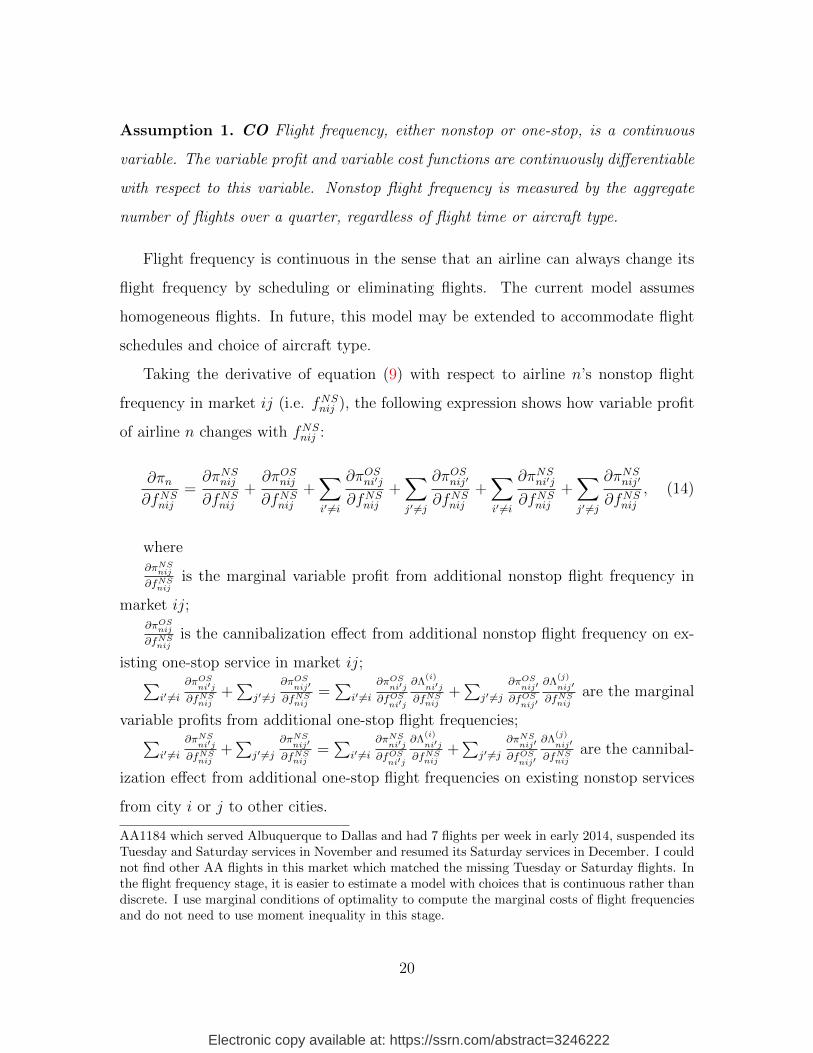
Taking the derivative of equation (9) with respect to airline n’s nonstop flight
frequency in market ij (i.e. fNSnij ), the following expression shows how variable profit
of airline n changes with fNSnij :
∂πn∂fNSnij
=∂πNSnij∂fNSnij
+∂πOSnij∂fNSnij
+∑i′ 6=i
∂πOSni′j∂fNSnij
+∑j′ 6=j
∂πOSnij′
∂fNSnij
+∑i′ 6=i
∂πNSni′j∂fNSnij
+∑j′ 6=j
∂πNSnij′
∂fNSnij
, (14)
where∂πNSnij∂fNSnij
is the marginal variable profit from additional nonstop flight frequency in
market ij;∂πOSnij∂fNSnij
is the cannibalization effect from additional nonstop flight frequency on ex-
isting one-stop service in market ij;∑i′ 6=i
∂πOSni′j
∂fNSnij+∑
j′ 6=j∂πOSnij′
∂fNSnij=∑
i′ 6=i∂πOSni′j
∂fOSni′j
∂Λ(i)
ni′j∂fNSnij
+∑
j′ 6=j∂πOSnij′
∂fOSnij′
∂Λ(j)
nij′
∂fNSnijare the marginal
variable profits from additional one-stop flight frequencies;∑i′ 6=i
∂πNSni′j
∂fNSnij+∑
j′ 6=j∂πNSnij′
∂fNSnij=∑
i′ 6=i∂πNSni′j
∂fOSni′j
∂Λ(i)
ni′j∂fNSnij
+∑
j′ 6=j∂πNSnij′
∂fOSnij′
∂Λ(j)
nij′
∂fNSnijare the cannibal-
ization effect from additional one-stop flight frequencies on existing nonstop services
from city i or j to other cities.
AA1184 which served Albuquerque to Dallas and had 7 flights per week in early 2014, suspended itsTuesday and Saturday services in November and resumed its Saturday services in December. I couldnot find other AA flights in this market which matched the missing Tuesday or Saturday flights. Inthe flight frequency stage, it is easier to estimate a model with choices that is continuous rather thandiscrete. I use marginal conditions of optimality to compute the marginal costs of flight frequenciesand do not need to use moment inequality in this stage.
20

Electronic copy available at: https://ssrn.com/abstract=3246222
Figure 1: Four Channels of Variable Profit Change
(a) Additional Nonstop(b) Cannibalization onOne-stop
(c) Additional One-stop
(d) Cannibalization onNonstop
Again, in these expressions, Λ(k)nij = Λ
(k)nij(f
NSnik , f
NSnkj ) denotes the one-stop flight
frequency from city i to city j with a connection at city k, where fNSnik and fNSnkj
represent flight frequency in market ik and market kj, respectively.
The six sub-figures in Figure 1 correspond to the four different channels. This is
a unique property of network models.
21
Electronic copy available at: https://ssrn.com/abstract=3246222
2.4.2 Computation of Counterfactual Network Structure
To estimate entry costs and the variable cost for additional flight frequency, as well
as to conduct a counterfactual experiment, I need to know how an airline’s network
structure will change when it enters/exits a market or changes its flight frequency in
a market, i.e., the counterfactual network structure. Let {FNSn ,FOS
n } denote airline
n’s network structure and F−n denote competitors’ network structures. Suppose
airline n changes its nonstop flight frequency from FNSn to FNS′
n , according to the
technological relationship between nonstop service and one-stop service, its one-stop
flight frequency changes according to the following technological function FOS′
n =
Λn(FNS′
n ).
Let FNSn ±fNSnij (FOS
n ±fNSnij ) denote the counterfactual nonstop (one-stop) flight fre-
quency structure of airline n if its nonstop flight frequency in market ij increases/decreases
by fNSnijt. Specifically, let FNSn ± 1NSnij (FOS
n ± 1NSnij ) denote the counterfactual nonstop
(one-stop) flight frequency structure of airline n if its nonstop flight frequency in
market ij increases or decreases by one.
3 Data
My sample includes the 100 busiest airports in the continental U.S., aggregated into
87 Metropolitan Statistic Areas (or cities).14 In each quarter, every airline makes
M = C×(C−1)2
= 3741 entry decisions.
The working dataset consolidates three databases: Data Bank 1B (DB1B), OAG
databases and Airport Gate database. DB1B is part of TranStats, the Bureau of
Transportation Statistics’ (BTS) online collection of databases, which contains a 10%
sample of all US domestic ticket information. The Official Airline Guide (OAG)
database contains all domestic flight schedules in the United States. I use all flight
scheduling and flight frequency information to construct measures of one-stop flight
14Some cities have more than one airport.
22

Electronic copy available at: https://ssrn.com/abstract=3246222
frequencies. I also construct an Airport Gate database which contains all airport
gate usage information. This information is collected from a flight statistics website
that reports daily domestic flight departure and arrival gate information.15 Since this
dataset identifies which airlines are using which gate, it can be used to determine
whether a gate belongs solely to one airline or is a common use gate.16 The unit of
observation in my working dataset is year-quarter-market-airline-product.
The working dataset ranges from the first quarter of 2007 to the fourth quarter of
2014 for a total of 32 quarters and 341110 observations.17
3.1 Descriptive Analysis
At the beginning of the sample period, 12 major airlines operate in the United States.
Virgin America enters in 2008.18 After several major mergers, there are nine major
airlines at the end of this sample period.19
Table 1 reports the number of nonstop (one-stop) markets in which the airline
operates, the share of nonstop (one-stop) passengers, and the percentage of revenue
from nonstop (one-stop) service. Legacy carriers usually operate direct flights in 200-
300 markets. Given these direct flight offerings, they can provide one-stop services in
thousands of markets.
Revenues from one-stop service tend to comprise a substantial portion of airline
15Domestic flight departure and arrival gate information are collected fromhttp://www.flightstats.com/. I use a Python to collect the departure and arrival gates of allflights in the United States in 2014.
16A gate is considered to belong to one airline if 80% of the flights departing from this gate areprovided by that particular airline. Otherwise, it is considered a common gate.
17Standard sample selection thresholds apply. All code-sharing tickets are dropped.18Virgin America begins its commercial service in late 2007 but enters my dataset in 2008.19Merger and dataset construction details can be found in Appendix A. I drop small airlines
such as Allegiant Air from the estimation and focus on the major airlines for three reasons: First,small airlines tend to concentrate their services in small markets and have negligible presence inthe sample dataset. Second, most of these small airlines employ a point-to-point business modeland usually carry a negligible proportion of connecting passengers. Third, eliminating these airlinescan save substantial computational time which is proportional to the number of airlines in thedataset. During the sample periodm, Continental merged with United Airlines, AirTran mergedwith Southwest, Northwest merged with Delta Air Lines, and US Airways merged with AmericanAirlines.
23

Electronic copy available at: https://ssrn.com/abstract=3246222
Table 1: Summary Statistics: Nonstop Service versus One-stop Service
2007Q1
Nonstop Service One-stop ServiceAirline Code (Name) # Markets % of Pass % of Rev # Markets % of Pass % of RevWN (Southwest Airlines) 364 84.7% 87.9% 1215 15.3% 12.1%DL (Delta Air Lines) 322 60.5% 76.3% 3529 39.5% 23.7%US (US Airway) 287 73.2% 82.3% 2318 26.8% 17.7%AA (American Airlines) 265 67.8% 78.3% 3009 32.2% 21.7%NW (Northwest Airlines) 207 65.9% 79.9% 3038 34.1% 20.1%UA (United Airlines) 202 73.1% 82.2% 2615 26.9% 17.8%CO (Continental Airlines) 186 78.5% 86.8% 2471 21.5% 13.2%FL (AirTran Airways) 95 67.7% 78.9% 681 32.3% 21.1%B6 (JetBlue Airways) 67 87.0% 92.1% 614 13.0% 7.9%F9 (Frontier Airlines) 46 69.7% 77.6% 900 30.3% 22.4%AS (Alaska Airlines) 45 96.4% 97.6% 209 3.6% 2.4%NK (Spirit Airlines) 22 100.0% 100.0% 53 0.0% 0.0%VX (Virgin America) - - - - - -Total 2108 74.9% 83.0% 20652 25.1% 17.0%
2014Q1
Nonstop Service One-stop ServiceAirline Code (Name) # Markets % of Pass % of Rev # Markets % of Pass % of RevWN (Southwest Airlines) 521 78.6% 84.6% 2274 21.4% 15.4%DL (Delta Air Lines) 421 58.6% 74.3% 3473 41.4% 25.7%US (US Airway) - - - - - -AA (American Airlines) 431 62.5% 75.8% 3347 37.5% 24.2%UA (United Airlines) 347 80.8% 89.7% 2675 19.2% 10.3%NW (Northwest Airlines) - - - - - -CO (Continental Airlines) - - - - - -FL (AirTran Airways) - - - - - -B6 (JetBlue Airways) 91 95.4% 97.3% 662 4.6% 2.7%F9 (Frontier Airlines) 43 58.4% 70.5% 567 41.6% 29.5%AS (Alaska Airlines) 62 98.4% 98.8% 370 1.6% 1.2%NK (Spirit Airlines) 65 97.2% 97.8% 136 2.8% 2.2%VX (Virgin America) 26 95.7% 97.1% 101 4.3% 2.9%Total 2007 71.9% 81.3% 13605 28.1% 18.7%Note: Pass is abbreviation of passengers and Rev is abbreviation of revenue.
24
Electronic copy available at: https://ssrn.com/abstract=3246222
profit. In the first quarter of 2014, Delta Air Lines brought in 23.7 percent of its
domestic revenue from one-stop service. Even Southwest, well-known for employing
a point-to-point business model, provides one-stop service to 15.3 percent of its con-
sumers and brings in 12.1 percent of its revenue from one-stop service.20 On average,
airlines provide one-stop service to 25.1 percent of their domestic passengers and bring
in 17 percent of their revenue from one-stop service. One-stop service is therefore an
important portion of airline operation and competition that should not be ignored.
3.2 Measure of Nonstop Flight Frequency
Nonstop flight frequency measures the number of daily direct flights offered by an
airline between two cities in a quarter. On average, an airline schedules 7.4 daily
direct flights in a market with a median of 5.5. Southwest operates in the busiest
nonstop market, connecting Southern California and the Bay area, with over 108
daily flights.
3.3 Hub cities
Airlines can connect one-stop passengers only at airline hubs. A list of airline hubs
is given in the Appendix. In the dataset, over 90% of the one-stop passengers travel
with a stop at hub cities.21
Table 2 lists the top two hubs and the operation concentration ratio at the top
four airports for each airline. I define the hub index of airline n at city i (Hni) as
the number of nonstop markets connected to city i. The operation concentration
ratio of an airline at a city is defined as its hub index at this city divided by the
number of direct markets of this airline. This ratio measures degree of ‘hubbing’ or
20A point-to-point business model is often employed by low-cost-carriers, who do not have majorhubs. Airlines using point-to point business models tend to provide direct service to passengers.
21I allow airlines to connect one-stop passengers only at hub cities so as to not over-estimateone-stop flight frequencies. To see these, suppose an airline has two hubs: A and B, both of whichconnect to spoke city C. I may conclude that there are many one-stop flights between A and B witha stop at C, though in fact no passengers connect at spoke city C.
25

Electronic copy available at: https://ssrn.com/abstract=3246222
Table 2: Summary Statistics: Hub City
2007Q1
Airline Code (Name) Top Hub #Mkts Second Hub #Mkts CR1 CR2 CR3 CR4
WN (Southwest Airlines) Chicago 47 Las Vegas 45 12.9 25.0 35.4 44.8DL (Delta Air Lines) Atlanta 83 Cincinnati 73 26.3 49.1 63.6 77.5US (US Airway) Charlotte 61 Philadelphia 54 22.3 41.8 57.9 70.0AA (American Airlines) Dallas 75 Chicago 71 28.8 55.8 68.8 81.5UA (United Airlines) Chicago 55 Denver 44 33.1 59.0 78.9 89.8NW (Northwest Airlines) Detroit 56 Minneapolis 55 36.1 71.0 91.0 96.8CO (Continental Airlines) Houston 46 New York 37 47.4 84.5 96.9 100.0FL (AirTran Airways) Atlanta 37 Orlando 18 38.9 56.8 67.4 74.7B6 (JetBlue Airways) New York 36 Boston 19 53.7 80.6 91.0 97.0F9 (Frontier Airlines) Denver 44 - 3 95.7 100.0 100.0 100.0AS (Alaska Airlines) Seattle 22 Portland 14 48.9 77.8 91.1 97.8NK (Spirit Airlines) - - - - 45.5 77.3 90.9 90.9VX (Virgin America) - - - - - - - -
2014Q2
Airline Code (Name) Top Hub #Mkts Second Hub #Mkts CR1 CR2 CR3 CR4
WN (Southwest Airlines) Chicago 62 Las Vegas 51 11.7 21.2 30.2 39.1DL (Delta Air Lines) Atlanta 82 Detroit 69 19.7 36.0 51.3 65.5US (US Airway) - - - - - - - -AA (American Airlines) Dallas 72 Charlotte 69 16.3 31.7 45.5 58.6UA (United Airlines) Chicago 58 Houston 43 22.5 38.8 53.9 68.2NW (Northwest Airlines) - - - - - - - -CO (Continental Airlines) - - - - - - - -FL (AirTran Airways) - - - - - - - -B6 (JetBlue Airways) New York 33 Boston 32 34.4 66.7 76.0 84.4F9 (Frontier Airlines) Denver 40 - 9 76.9 92.3 94.2 98.1AS (Alaska Airlines) Seattle 35 Portland 20 50.0 77.1 85.7 91.4NK (Spirit Airlines) - - - - 26.0 45.5 59.7 72.7VX (Virgin America) San Francisco 14 Los Angeles 12 53.8 96.2 100.0 100.0
26

Electronic copy available at: https://ssrn.com/abstract=3246222
concentration of an airline’s operations in a given city and equals one for pure hub-
and-spoke networks. The top two hubs of legacy carriers usually connect with over
60 other cities and have high hub concentration ratios. Frontier Airlines employs a
nearly perfect hub-and-spoke network.22 Southwest Airlines has the lowest operation
concentration ratio. In 2007, its top hub (Chicago) connected with 47 other cities, its
second hub (Las Vegas) connected with 45 other cities, and its CR4 was less than 40,
which is consistent with the fact that the airline employs a point-to-point business
model.
Some airlines expand their hubs during the sample period. For instance, Alaska
Airlines increased its nonstop service in Seattle from 22 to 35. Southwest increased its
nonstop markets in Chicago from 47 (2007) to 62 (2014). There has been a reduction
in hub concentration ratios from 2007 to 2014 due to several major mergers, since the
merged airlines have a greater number of hubs.
3.4 Measure of One-stop Flight Frequency
One-stop service introduces important interconnections between airline operation de-
cisions across markets.23 In this paper, I propose a new measure of one-stop flight
frequency based on airline schedules, flight frequencies and the technology of connect-
ing service.
I measure one-stop flight frequency from city A to city C with a connection at city
B as follows. Suppose an airline schedules a first flight from city A to city B, and a
second flight from city B to city C. These two direct flights are considered to create
a one-stop flight if the scheduled departure time of second flight is anywhere from 45
minutes to 4 hours after the scheduled arrival time of the first flight.24 When there
22In a perfect hub-and-spoke network, there is a sole hub city and there are direct flights fromother cities to the hub city.
23Previous literature measures one-stop service in a relatively simple way and assumes an airlineprovides one-stop service in a market if the number of one-stop passengers exceeds a threshold.However, this measure is an equilibrium result from a 10 percent sample and ignores heterogeneityin one-stop service.
24I use the same threshold (45 minutes to 4 hours) as in Molnar (2013). The minimum time for
27

Electronic copy available at: https://ssrn.com/abstract=3246222
are multiple flights in market AB connecting with multiple flights in market BC, the
one-stop flight frequency is the total number of connecting possibilities available to
one-stop passengers. The detailed algorithm is described in detail in Appendix.
To the best of my knowledge, no measures of one-stop flight frequency have been
proposed in the literature. This measure introduces a clear definition of airline entry
with one-stop service (two flights with a layover of 45 minutes to 4 hours) as well as
heterogeneity or quality in one-stop service (measured by one-stop flight frequencies).
This measure is important for understanding competition and profitability in this
industry. Airlines can receive more revenue from one-stop service if they construct
their networks strategically and increase one-stop flight frequency. They also face
more intensive competition if their competitors have more one-stop flight frequencies.
There are 273814 airline-market-quarter observations with positive flight frequency
for one-stop service. On average, an airline carries 6.8 one-stop passengers between
two cities on a daily basis with a median of 2.5.
4 Empirical Implementation
This section discusses the empirical specification of the network competition model. I
first specify the entry cost of the airlines, followed by the variable costs, which include
the variable cost of scheduling flights and serving passengers. Finally, I discuss the
demand model and technological relationship between nonstop and one-stop flight
frequencies.
4.1 Entry cost
Airline n’s entry cost into market ij in quarter t (FCnijt) depends upon many factors,
such as the number of gates or time slots of the airline at the two endpoint cities,
domestic connection is usually 45 to 75 minutes. The maximum time for domestic connection isusually 4 hours.
28

Electronic copy available at: https://ssrn.com/abstract=3246222
etc.25
I specify FCnijt as follows
FCnijt = γFCG (Gnit +Gnjt)︸ ︷︷ ︸Gate Share at the Airport
+ ηFCn︸︷︷︸Airline FE
+ ηFCt︸︷︷︸Quarter FE
+ ηFCi + ηFCj︸ ︷︷ ︸City FE
+ εFCnijt, (15)
where ηFCn represents airline fixed-effect, ηFCt represents quarter fixed-effect, ηFCi and
ηFCj represent city fixed-effects at the two endpoints of the market, Gnit and Gnjt are
the share of gates leased to airline n at city i and j in quarter t, respectively. So
ηFCt /100 measures how fixed cost changes if the gate share of the airline at an airport
increases by 1%.
4.2 Variable Costs
This paper distinguishes two different types of variable costs of the airlines: variable
cost of scheduling flights and variable cost of serving passengers.
Variable Cost of Scheduling Flights
I assume variable cost of scheduling flights is proportional to flight frequency, i.e.
V Cfnijt(f
NSnijt) = cfnijt × fNSnijt. Marginal cost of flight frequency (cfnijt) is given by
ln cfnijt = γfH(Hnit +Hnjt)︸ ︷︷ ︸Hub Indexes
+ γf1 dij + γf2 d2ij︸ ︷︷ ︸
Distance
+ ηfni + ηfnj︸ ︷︷ ︸Airline-City FE
+ ηft︸︷︷︸Quarter FE
+ εfnijt, (16)
where γfH measures changes in variable cost of flight frequency if hub index increases
by one. Hnit and Hnjt are the hub indexes of the airline at the two endpoints. ηfni
and ηfnj are airline-city fixed effect, ηft is time fixed-effects and γf1 and γf2 capture the
effect from distance.
25Ciliberto and Williams (2010) find that cost of entry decrease with the number of gates anairline operates in an airport.
29

Electronic copy available at: https://ssrn.com/abstract=3246222
Variable Cost of Serving Passengers
In the empirical specification, a product g represents the following four-tuple of market
and product characteristics: (1) airline n, (2) market ij, (3) quarter t and (4) nonstop
product indicator variable x.
Marginal cost of serving passengers who travel with product g (cg) is given by
cg = δ11[x = NS]︸ ︷︷ ︸Nonstop Dummy
+ δ2l(fNSg
)× 1[x = NS] + δ3l
(fOSg
)× 1[x = OS]︸ ︷︷ ︸
Flight Frequency
(17)
+δ3Hnit + δ4Hnjt︸ ︷︷ ︸Hub Indexes
+ δ5dij + δ6d2ij︸ ︷︷ ︸
Distance
+ ω(1)ni + ω
(2)nj︸ ︷︷ ︸
Airline-City FE
+ ω(3)t︸︷︷︸+ω(4)
g
Quarter FE
,
where δ1 measures the cost difference between nonstop and one-stop services, l (fg)
is a non-decreasing function of fg, Hnit and Hnjt are airline hub indexes at each
respective endpoint, ω(1)ni and ω
(2)nj are airline-city fixed-effects, ω
(3)t represents quarter
fixed-effects, and ω(4)g is product-specific cost shock.26
4.3 Demand Model
Product quality, bg, is given by:
bg = α11[x = NS]︸ ︷︷ ︸Nonstop Dummy
+ α2l(fNSg )× 1[x = NS] + α3l(f
OSg )× 1[x = OS]︸ ︷︷ ︸
Flight Frequencies
(18)
+α4Hnit + α5Hnjt︸ ︷︷ ︸Hub Indexes
+ α6dij + α7d2ij︸ ︷︷ ︸
Distance
+ ξ(1)n︸︷︷︸
Airline FE
+ ξ(2)i + ξ
(3)j︸ ︷︷ ︸
City FE
+ ξ(4)t︸︷︷︸
Quarter FE
+ ξ(5)g ,
where α1 measures average passenger utility from nonstop service over the utility
of one-stop service; Hnit and Hnjt are hub indexes at the two endpoint cities; ξ(1)n
is an airline fixed-effects which captures between-airlines differences in quality that
26Empirically, I define l(fg) = ln(14× fg − 13) to ensure variable profit is a concave function withrespect to flight frequency. Since the minimum daily flight frequency in this paper is one, l(1) = 0.Suppose I choose l(fg) = ln(fg) or l(fg) = fg, variable profit is a convex function of fg and airlinesshould schedule an infinite number of flights in this market.
30

Electronic copy available at: https://ssrn.com/abstract=3246222
are constant over time and across markets; ξ(2)i and ξ
(3)j are city fixed-effects; ξ
(4)t is
quarter fixed-effects; ξ(5)g is product-specific demand shock for product g.27
I consider a nested logit demand model with two nests.28 The first nest represents
the consumer decision of which airline to travel with, while the second nest is the
choice between nonstop and one-stop flights. Suppose vιg = σ1v(1)ιnijt + σ2v
(2)g , where
v(1)ιnijt and v
(2)g are independently Type 1 extreme value distributed, and σ1 and σ2 are
parameters which measure within/between group substitutions.
Let sg denote the market share of product g in market ij, i.e., sg = qg/MSij. Let
s∗g be the within group market share of product g, i.e., s∗g = sg/∑
g′∈Ggsg′ , where Gg
is the set of products airline n offers in the same market as product g.
The demand system can be represented using the following closed-form demand
equations. For each g
ln(sg)− ln(s0) =bg − pgσ1
+ (1− σ2
σ1
)ln(s∗g). (19)
4.4 Technological Relationship between One-stop and Non-
stop Flight Frequencies
I assume airline n’s one-stop flight frequency between city i and j with a stop at
city k in quarter t (fOS(k)nijt ) is a symmetric Cobb-Douglas function with respect to its
nonstop flight frequencies in market ik (fNSnikt) and market kj (fNSnkjt).
fOS(k)nijt = Λ
(k)nijt
(fNSnikt, f
NSnkjt
)= exp
(h
(k)nijt
)×(fNSnikt
)λ × (fNSnkjt
)λ, (20)
where h(k)nijt measures the heterogeneity in connection technologies across the one-stop
markets. Furthermore, I specify h(k)nijt = h + ε
h(k)nijt , where ε
h(k)nijt is assumed to be i.i.d
27These hub indexes are measured by the number of nonstop markets an airline serves to otherdestinations.
28The model can be extended into a random coefficient model.
31

Electronic copy available at: https://ssrn.com/abstract=3246222
distributed with mean zero and thus obtain the following regression equation:
ln fOS(k)nijt = h+ λ×
(ln fNSnikt + ln fNSnkjt
)+ ε
h(k)nijt . (21)
This technological model predicts counterfactual network structure given nonstop
flight frequency changes. Specifically, when nonstop flight frequency in market ik
changes, one-stop flight frequency in market ij with a stop at city k changes according
to the following equation:
∂fOS(k)nijt
∂fNSnikt
= λ×fOS(k)nijt
fNSnikt
. (22)
5 Identification and Estimation
This section discusses the empirical strategy and identification assumptions. The
three-stage model is estimated sequentially. I first estimate consumers’ utility func-
tions and back out airlines’ marginal cost of serving consumers according to Bertrand
Nash conditions. Then, I estimate airlines’ marginal cost of flight frequencies accord-
ing to marginal conditions of optimality for flight frequency choice. The estimation
of airline entry cost suffers from high dimensionality in strategy space and it is im-
possible to compute a Nash equilibrium. My empirical strategy is based on partial
identification: I treat the observed network structure as a Nash equilibrium outcome.
Airlines’ revealed preference in entry decisions generates a set of inequality restrictions
on entry cost. I infer entry cost exploiting these inequality restrictions.
5.1 Estimation of Demand and Variable Cost of Passengers
According to the quality specification in Equation (18) and demand system in Equa-
tion (19), the demand model can be expressed as a linear-in-parameters system of
32
Electronic copy available at: https://ssrn.com/abstract=3246222
equations represented by:
ln(sg)− ln(s0) = Wgα−pgσ1
+ (1− σ2
σ1
)ln(s∗g) + ξ(4)g , (23)
where Wg is a vector of regressors that includes a nonstop product dummy, functions
with respect to flight frequencies in both nonstop and one-stop services, hub indexes
at the two endpoint cities, distance between two endpoint cities, airline dummies, city
dummies and quarter dummies. In this regression equation, price pg and conditional
market share ln(s∗g) are endogenous. Products with larger demand shocks (ξ(4)g ) are
more likely to have higher prices as well as higher conditional market shares. More-
over, airline flight frequency may be an endogenous regressor in the current demand
system because airlines may schedule more flights in markets with higher demand.
I impose two assumptions to construct valid instrumental variables to identify
demand.
Assumption 2. INDEPENDENT ξ Product-specific demand shocks {ξ(4)g } are
independently distributed over time.
Assumption 3. TIME-TO-BUILD At the beginning of quarter t, airlines form
expectations about demand and costs before making their entry and flight frequency
decisions in all markets. These entry and flight frequency decisions are not effective
until quarter t + 1 because airlines require one quarter to set up their networks and
schedule their flights.
Assumption INDEPENDENT ξ establishes that, after controlling for airline
fixed-effects, time fixed-effects and market fixed-effects, the unobserved component of
product demand does not exhibit time dependence. Assumption TIME-TO-BUILD
assumes that airline network structure at quarter t is pre-determined in quarter t−1,
before demand shocks at quarter t are realized.29 These two assumptions imply
29These two identification assumptions are in the same spirit as those in the estimation of demandin Aguirregabiria and Ho (2012) and Sweeting (2013).
33

Electronic copy available at: https://ssrn.com/abstract=3246222
that demand shock ξ(4)g is independent of airline market entry and flight frequency
decisions.30
I use GMM to estimate the differentiated products demand systems. Charac-
teristics of other products in the same market are used as instruments.31 In the
current model, instrument variables include average flight frequencies in both non-
stop and one-stop services, hub indexes at both origin and destination cities and
nonstop product dummies of competing products. These two assumptions establish
that product characteristics of competitors in quarter t are independent of demand
shock ξ(4)g because they are pre-determined in quarter t − 1. Moreover, competitor
product characteristics are correlated with product price through price competition,
but are not correlated with product-specific demand shocks. Thus, they can be valid
instruments for both prices pg and within nested market share ln(s∗g).
Given estimates of demand parameters and under Nash-Bertrand competition
assumptions, I back-out marginal cost of serving passengers from cg = pg − σ1(1 −
sg)−1.32 I further decompose variable cost of serving passengers to factors listed in
Equation (17). Assuming no further issues of endogeneity, I use OLS to estimate
marginal cost of serving passengers.
5.2 Estimation of Marginal Cost of Flight Frequencies
I infer cost of flight frequency from demand estimation. After obtaining estimates of
consumer utility and airline marginal cost of serving passengers, I back out marginal
cost of flight frequency (cfnijt) according to marginal conditions of optimality for flight
frequency choice. Setting the expected marginal variable profit from additional flight
frequency ( ∂πnt∂fNSnijt
) equal to the marginal cost of scheduling additional flight frequency
30Assumption INDEPENDENT ξ is testable. I test this assumption with estimated residuals
ξ(4)g from a GMM estimation of the demand system.31This is in the spirit of Berry (1992) and Berry, Levinsohn, and Pakes (1995).32sg = (
∑g′∈Gnijt
eg′)σ2σ1 [1 +
∑Nn′=1(
∑g′∈Gn′ijt
eg′)σ2σ1 ]−1 where eg = Igexp{(bg − pg)/σ1} and Ig
is the indicator of the event “product g is available or not”.
34

Electronic copy available at: https://ssrn.com/abstract=3246222
(cfnijt) gives:
∂πnt(FNSnt ,F
OSnt )
∂fNSnijt
= cfnijt. (24)
Thus, the regression equation becomes
ln∂πnt∂fNSnijt
= γfH(Hnit +Hnjt)︸ ︷︷ ︸Hub Indexes
+ γf1 dij + γf2 d2ij︸ ︷︷ ︸
Distance
+ ηfni + ηfnj︸ ︷︷ ︸Air-City FE
+ ηft︸︷︷︸Qtr FE
+ εfnijt. (25)
The value of ∂πnt∂fNSnijt
is numerically computed from
∂πnt∂fNSnijt
=πnt(F
NSnt + 1NSnijt,F
OSnt + 1NSnijt)− πnt(FNS
nt − 1NSnijt,FOSnt − 1NSnijt)
2, (26)
where, as described in Section 2.4.2, πnt(FNSnt +1NSnijt,F
OSnt +1NSnijt) is the variable profit
of airline n if it increases its nonstop flight frequency in market ij in quarter t by 1
while πnt(FNSnt − 1NSnijt,F
OSnt − 1NSnijt) is the variable profit of airline n if it reduces its
nonstop flight frequency in market ij in quarter t by 1.
5.3 Estimation of Entry Cost
Having obtained estimates for demand and marginal costs, I now turn my attention
to the parameters governing fixed cost. These parameters show the heterogeneity in
entry cost for airlines with different numbers of gates at airports and heterogeneity
across airlines, quarters, and cities. Traditional estimation methods for entry models
are unfeasible in my case: the total number of cities and airlines implies too large a
state space to be solved numerically. To circumvent this curse of dimensionality, I
approach the problem using a partial identification approach.
35

Electronic copy available at: https://ssrn.com/abstract=3246222
5.3.1 Two Sets of Inequality
I use two sets of moment inequality to construct bounds on the fixed cost. If airline
n operates direct flight in a market ij, its entry cost into this market is lower than
the difference between variable profit in the observed network πnt(FNSnt ,F
OSnt
)and
the counterfactual variable profit if it does not operate direct flight in this market
πnt(FNSnt − fNSnijt,F
OSnt − fNSnijt
)minus savings in variable cost of flight frequency cfnijt×
fNSnijt.33 Thus,
FCnijt ≤ πnt(FNSnt ,F
OSnt
)︸ ︷︷ ︸Observed Var Profit
− πnt(FNSnt − fNSnijt,F
OSnt − fNSnijt
)︸ ︷︷ ︸Counterfactual Var Profit if Exit
− cfnijt × fNSnijt︸ ︷︷ ︸Cost (Frequency)
(27)
≡ FCnijt,
where FNSnt − fNSnijt (FOS
nt − fNSnijt) denotes the counterfactual nonstop (one-stop) flight
frequencies network structure if airline n exits market ij. This is an upperbound for
fixed cost.
If airline n does not operate direct flights in market ij, its entry cost into market ij
is higher than the difference between counterfactual variable profit πnt(FNSnt + fNS∗nijt ,F
OSnt + fNS∗nijt
)if it enters with optimal flight frequency fNS∗nijt and the variable profit in the observed
network πnt(FNSnt ,F
OSnt
)minus variable cost of building flight frequencies cfnijt×fNS∗nijt .
FCnijt ≥ maxfNSnijt
πnt(FNSnt + fNSnijt,F
OSnt + fNSnijt
)︸ ︷︷ ︸Var Profit if Optimal Frequency Entry
− πnt(FNSnt ,F
OSnt
)︸ ︷︷ ︸Observed Var Profit
− cfnijt × fNSnijt︸ ︷︷ ︸Cost (Frequency)
(28)
≡ FCnijt,
where FNSnt + fNSnijt (FOS
nt + fNSnijt) denotes the counterfactual nonstop (one-stop) flight
frequencies in all markets if airline n exits market ij. When airline n determines its
flight frequency in market ij, it will take into account its entire network structure
and maximize its total variable profit in the network. This generates a lowerbound
33FNSnt − fNS
nijt is the counterfactual nonstop flight frequency if airline n exits market ij and
FOSnt − fNS
nijt is the counterfactual one-stop flight frequency if airline n exits market ij.
36

Electronic copy available at: https://ssrn.com/abstract=3246222
for fixed cost.
5.3.2 Identification Issues and Assumptions
There are two identification issues in the estimation of entry cost. First, given that
an airline is active in a market, it may own, lease or operate more gates at the two
endpoints of the market. As a result, the share of gates an airline leasing at an airport
may be endogenous. The following identification assumption is imposed to ensure the
consistency of the fixed cost estimates.
Assumption 4. GATE The number of gates an airline has at an airport is exoge-
nous. Airlines determine their gate allocations before they determine their network
structures.
Assumption GATE is reasonable because gate leasing arrangements between air-
lines and airports are usually signed several years before the airline’s operation deci-
sions. Thus, the entry decision of an airline into a market will not affect the percentage
of gates an airline leases at the airport.
The second issue is selection associated with random disturbance. The random
disturbance associated with the observed choice comes from the possible values that
make the observed choice the optimal choice. As a result, even though a priori mean
of the random disturbance for any fixed choice is zero, the mean of the random
disturbance may be nonzero. In other words, airlines that are active in a market may
have received a good draw, i.e. E[εFCnijt|Xnijt, anijt = 1
]≥ 0. In contrast, airlines that
are inactive in a market may have receive a bad draw, i.e. E[εFCnijt|Xnijt, anijt = 0
]≤ 0.
In order to deal with this selection issue and obtain consistent estimates of parameters
in the entry cost function, I impose the following identification assumption.
Assumption 5. BOUND The conditional expectation of εFCnijt is finite
Under Assumption BOUND, there is a finite bound B such that |E[εFCnijt|anijt =
37

Electronic copy available at: https://ssrn.com/abstract=3246222
1]| ≤ B and |E[εFCnijt|anijt = 0]| ≤ B.34
When the distribution of the error term is not specified, the true value of B is
unknown and selection of B becomes an empirical question. I evaluate the fit of the
model at different values of B and select a B = B∗ such that the model estimates
optimize the overall fit of the model. Details on how I select B are in Section 5.3.5.
5.3.3 Estimation Procedure
I restrict my analysis to 2014 data for which detailed gate operation information are
available. If I observe an airline is active in a market, I have an upperbound for fixed
cost. Conversely, if I observe an airline is not active in a market, I have a lowerbound
for fixed cost. There are 6934 upperbounds and 14626 lowerbounds for entry cost.35
There are one hundred parameters (or fixed-effects) in the entry cost function. I
estimate all parameters simultaneously using Inequalities (27) and (28). However,
estimation of one hundred parameters with thousands of inequality may result in
imprecise and uninformative estimates. Moreover, there may be numerical errors
when I estimate a model with one hundred parameters as the optimizing algorithm
may stop at a local minimum rather than global minimum.36 Therefore I propose
a sequential estimation procedure and obtain estimates of different sets of fixed cost
parameters sequentially.
An overview of this estimation procedure is as follows: I first estimate the effects
from gate ownership on fixed cost (γFCG ). When an airline is active in market ij
but inactive in market i′j′ and another airline is inactive in market ij but active in
market i′j′ in the same quarter, the difference in their entry decisions comes from
34Pakes, Porter, Ho, and Ishii (2015) and Ellickson, Houghton, and Timmins (2013) assume thatafter controlling for firm fixed-effects and market fixed-effect, conditional expectation of the errorterms have mean zero. This is a special case when B = 0.
35This paper focuses on observations where an airline is active in a market or active in bothendpoints of the market. For an entry cost, I can either observe an upperbound or a lowerbound,because the airline can either be active or inactive.
36The criterion function is continuous but not differentiable. To search for a global minimum Imay have to start at trillions of initial values. For instance, for 100 parameters with ten values each,I would need to evaluate 10100 different initial values.
38

Electronic copy available at: https://ssrn.com/abstract=3246222
the difference in their gate allocations at different markets. I make use of Inequality
(27) and (28), construct swapping pairs, eliminate airline fixed-effects, quarter fixed-
effects, and city fixed-effect, and focus on a set of new inequality with only parameter
γFCG involved. After obtaining estimate γFCG , I replace the true γFCG with γFCG in both
sets of inequality and proceed to estimate quarter fixed-effects. If an airline is active in
a market in a quarter but inactive in the same market in another quarter, I can obtain
upper and lower bounds for quarter fixed-effects differences. I construct swapping
pairs, eliminate airline fixed-effects and city fixed-effects and obtain inequality with
only quarter fixed-effect γFCt , where I estimate and obtain γFCt . Then I replace the
true γFCt with estimates γFCt in the two sets of inequality and estimate airline fixed-
effects. If I observe an airline is active in a market and another airline is inactive in
the same market, I obtain bounds for the difference between the airlines’ fixed-effects
in fixed cost. I obtain inequality with only γFCn and obtain its estimate γFCn . Finally,
I estimate city fixed-effects. I replace the γFCG , γFCn , and γFCt with their estimates in
Inequality (27) and (28). The estimates of city fixed-effects minimize these two sets
of inequality.
The main advantage of this sequential estimation procedure is that I eliminate
some fixed-effects and focus on the estimation of a set of key parameters. There will
be less estimation error associated with these key parameters. However, a drawback
of this estimation procedure is that estimation error in earlier steps may propagate
to later steps.
Estimation of γFCG
When estimating γFCG , I construct incumbent and potential entrant pairs at two
markets to eliminate time fixed-effects, airline fixed-effects and market fixed-effects.
This swapping is in the spirit of Ellickson, Houghton, and Timmins (2013) and Pakes,
Porter, Ho, and Ishii (2015). Specifically, suppose airline n operates direct flights in
market ij but not in market i′j′ and airline n′ operates direct flights in market i′j′
39
Electronic copy available at: https://ssrn.com/abstract=3246222
but not in market ij.
Airline n receives positive profit in market ij
FCnijt − γFCG (Gnit +Gnjt)− (ηFCn + ηFCt + ηFCi + ηFCj + εFCnijt) ≥ 0. (29)
Airline n receives negative profit if it enters i′j′
γFCG (Gni′t +Gnj′t) + (ηFCn + ηFCt + ηFCi′ + ηFCj′ + εFCni′j′t)− FCni′j′t ≥ 0. (30)
Airline n′ receives negative profit if it enters ij
γFCG (Gn′it +Gn′jt) + (ηFCn′ + ηFCt + ηFCi + ηFCj + εFCn′ijt)− FCn′ijt ≥ 0. (31)
Airline n′ receive positive profit when it operates in i′j′
FCn′i′j′t − γFCG (Gn′i′t +Gn′j′t)− (ηFCn′ + ηFCt + ηFCi′ + ηFCj′ + εFCn′i′j′t) ≥ 0. (32)
Summing up (29) to (32) gives
∆FCn′i′j′tnijt − γFCG ∆Gn′i′j′t
nijt − εFCnijt + εFCni′j′t + εFCn′ijt − εFCn′i′j′t ≥ 0, (33)
where ∆FCn′i′j′tnijt ≡ FCnijt − FCni′j′t − FCn′ijt + FCn′i′j′t and ∆Gn′i′j′t
nijt ≡ Gnit +
Gnjt −Gni′t −Gnj′t +Gn′it +Gn′jt −Gn′i′t −Gn′j′t. All airline fixed-effects ηFCn , time
fixed-effects ηFCt and city fixed-effects ηi and ηj are canceled out in Inequality (33).
I transform these inequality to conditional moment inequality
E[∆FCn′i′j′tnijt − γFCG ∆Gn′i′j′t
nijt − εFCnijt + εFCni′j′t + εFCn′ijt − εFCn′i′j′t|Xt, At] ≥ 0, (34)
where Xt is a vector of market and airline characteristics, which include market size,
distance between endpoints and other explanatory variables for entry cost and At is
40

Electronic copy available at: https://ssrn.com/abstract=3246222
a vector of airline’s entry and exit decisions in quarter t.
Under Assumption Bound, I obtain the following inequality
E[∆FCn′i′j′tnijt − γFCG ∆Gn′i′j′t
nijt + 4B|Xt] ≥ 0 (35)
where ∆FCn′i′j′tnijt and ∆Gn′i′j′t
nijt are obtained in the data.37 When ∆Gn′i′j′tnijt is positive,
I have an upperbound for γFCG . Otherwise, I have a lowerbound for γFCG .
Andrews and Shi (2013) show that by properly choosing instruments, conditional
moment inequalities are transformed into their unconditional counterparts without
losing identification power. So the conditional inequality can be rewritten as the
following unconditional inequality
E{zG[∆FCn′i′j′tnijt − γFCG ∆Gn′i′j′t
nijt + 4B]} ≥ 0, (36)
where {zG} are non-negative instruments based on market characteristics.
Specifically, I separate all inequality into different groups and the instruments are
dummy variables indicating whether an inequality belongs to a group or not. All
inequality representing the upperbound of γFCG (those inequality with ∆Gn′i′j′tnijt > 0)
are aggregated to 4, 6, 8, 10, 12 and 14 groups. Again, all inequality representing the
upperbound of γFCG (those inequality with ∆Gn′i′j′tnijt < 0) are aggregated to 4, 6, 8,
10, 12 and 14 groups. The selection of groups are based on the quantiles of ∆Gn′i′j′tnijt .
For instance, when I separate all inequality into four groups (four different quantiles),
the first group includes all inequality whose ∆Gn′i′j′tnijt falls in its first quantile and the
last group includes those inequality whose ∆Gn′i′j′tnijt falls in its fourth quantile.
The criterion function follows Chernozhukov, Hong, and Tamer (2007):
Qγ =∑zG
min{∑t
∑n
∑n′ 6=n
∑ij
∑i′j′ 6=ij
zG[∆FCn′i′j′tnijt − γFCG ∆Gn′i′j′t
nijt + 4B], 0}2.(37)
37The absolute value of all conditional expectation of error terms |E[εFCnijt|Xt, At]| ≤ B.
41
Electronic copy available at: https://ssrn.com/abstract=3246222
I estimate γFCG to minimize the criterion function Qγ.
Estimation of Time Fixed-effects (ηFCt )
I estimate time fixed-effects by exploiting cross quarter entry decisions. In a given
market, if an airline n is active in this market in quarter t but not active in quarter
t′, I construct inequality, eliminate other fixed-effects and focus on the estimation of
time fixed-effects ηFCt .
Airline n receives positive profit when it operates in ij in t
FCnijt − γFCG (Gnit +Gnjt)− (ηFCn + ηFCt + ηFCi + ηFCj + εFCnijt) ≥ 0. (38)
Airline n receives negative profit if it enters ij in t′
γFCG (Gnit′ +Gnjt′) + (ηFCn + ηFCt′ + ηFCi + ηFCj + εFCnijt′)− FCnijt′ ≥ 0. (39)
Summing up these two inequality and replacing γFCG with estimates γFCG , I have
∆FCnijt′
nijt − γFCG ∆Gnijt′
nijt − ηFCt + ηFCt′ − εFCnijt + εFCnijt′ ≥ 0, (40)
where ∆FCnijt′
nijt ≡ FCnijt − FCnijt′ and ∆Gnijt′
nijt ≡ Gnit +Gnjt −Gnit′ −Gnjt′ .
Following the same steps as before, I have the following criterion function.
QT =∑zT
min{∑nij
∑t
∑t′ 6=t
zT [∆FCnijt′
nijt − γFCG ∆Gnijt′
nijt − ηFCt + ηFCt′ + 2B], 0}2.(41)
The ηFCt minimizes this criterion function. I normalize the first quarter fixed effect to
0. {zT} are dummy variables that select different combination of quarters. Since there
are four quarters in the working database, there are C42 = 12 different combinations.
42

Electronic copy available at: https://ssrn.com/abstract=3246222
Estimation of Airline Fixed-effects (ηFCn )
After obtaining estimates of quarter fixed-effects, I estimate airline fixed-effects by
exploiting variation in airlines’ entry decisions in the same market. For any two
airlines n and n′ in market ij, if n is active in the market but n′ is not active in
the same market, I construct inequalities and eliminate market fixed-effects and time
fixed-effects. Summing up (29) and (31) and replacing γFCG with its estimates, I obtain
∆FCn′ijtnijt − γFCG ∆Gn′ijt
nijt − ηFCn + ηFCn′ − εFCnijt + εFCn′ijt ≥ 0, (42)
where ∆FCn′ijtnijt ≡ FCnijt − FCn′ijt and Gn′ijt
nijt ≡ Gnit +Gnjt −Gn′it −Gn′jt. Again, I
have the following criterion function
QN =∑zN
min{∑ijt
∑n
∑n′ 6=n
zN [∆FCn′ijtnijt − γFCG ∆Gn′ijt
nijt − ηFCn + ηFCn′ + 2B], 0}2, (43)
where {zN} are indicator variables for all possible airline-pairs. I normalize the airline
fixed-effect of American Airline to 0 and estimate ηFCn to minimize this criterion
function.
Estimation of City Fixed-effects
To estimate city fixed-effects, I replace gate fixed-effects of gate (γFCG ), time fixed-
effects (ηFCt ) and airline fixed-effects (ηFCn ) with their estimates and estimate city
fixed-effects utilizing airline market entry decisions. For any market ij, if airline n is
active in quarter t, I obtain an upper bound for the city fixed-effect:
anijt(FCnijt − γFCG (Gnit +Gnjt)− (ηFCn + ηFCt + ηFCi + ηFCj + εFCnijt)) ≥ 0, (44)
43

Electronic copy available at: https://ssrn.com/abstract=3246222
whereas if airline n is not active in the same quarter, I obtain a lower bound for the
city fixed-effects.
(anijt − 1)(FCnijt − γFCG (Gnit +Gnjt)− (ηFCn + ηFCt + ηFCi + ηFCj + εFCnijt)) ≥ 0.(45)
Summing up these two inequality,
anijtFCnijt + (anijt − 1)FCnijt − (2anijt − 1)γFCG (Gnit +Gnjt) (46)
−(2anijt − 1)(ηFCn + ηFCt + ηFCi + ηFCj + εFCnijt) ≥ 0.
Again, estimates ηFCi minimize the following criterion function
QC =∑
anijt={0,1}
∑zC
min{∑nijt
zC [anijtFCnijt + (anijt − 1)FCnijt (47)
−(2anijt − 1)(γFCG + (Gnit +Gnjt) ηFCn + ηFCt + ηFCi + ηFCj ) +B], 0}2
where {zC} are indicator variables for different quantiles of market size.
The true γ values should satisfy all the inequality if the model is correctly specified.
If multiple (sets of) estimates satisfy all inequality (when γ = γ, the value of criterion
function = 0), then a set estimate is obtained. If there is no estimate that satisfies
all inequality (i.e. there is no γ = γ such that the value of criterion function = 0), I
select a γ that minimizes the criterion function as a point estimate. Thus, though a
set identification approach is being employed, it may still result in a point estimate.38
5.3.4 Computation of Goodness of Fit and the Selection of B∗
To estimate the entry cost, I first determine the value of B. Since the true value of
B is unknown, I numerically search for the optimal B∗ in the empirical analysis. I
try different values of B ranging from 0 to 1000 in steps of five. For any trial of B,
I estimate fixed cost according to the procedures described in Section 5.3.3. Then, I
38It is very difficult to describe a set estimate when there are 100 parameters.
44

Electronic copy available at: https://ssrn.com/abstract=3246222
predict airline entry decisions in all markets. According to Inequality (27), the model
predicts that an airline will enter the market if its expected variable profit is higher
than its estimated entry cost. On the other hand, according to Inequality (28), the
model predicts that the airline will not enter the market if its expected variable profit
is lower than its estimated entry cost. By comparing the predicted and observed entry
decisions, I compute overall model fit for the fixed cost estimates as the fraction of
model predictions that are consistent with airline entry/exit decisions in the data.
Finally, I select B∗ to maximize the overall fit of the model.
5.3.5 Estimation of SD of Individual Shock εFCnijt
In the counterfactual experiment, I simulate errors from the estimated distribution
of individual shocks. This subsection estimates the distribution of error terms in the
fixed cost. If airline n is active in ij, Inequality (29) imposes an upper bound for
εFCnijt. If airline n is active in ij in quarter t, I replace parameters with their estimates
and obtain
εFCnijt ≤ FCnijt − γFCG (Gnit +Gnjt)− ηFCn − ηFCt − ηFCi − ηFCj ≡ εFCnijt. (48)
Otherwise, Inequality (30) imposes a lower bound for εFCnijt. If airline n is inactive in
ij in quarter t,
εFCnijt ≥ FCnijt − γFCG (Gnit +Gnjt)− ηFCn − ηFCt − ηFCi − ηFCj ≡ εFCnijt. (49)
To identify the distribution of individual shocks from these two sets of inequality,
I impose the following assumption on the distribution of ε.
Assumption 6. ε Distribution Suppose εFCnijt is i.i.d normally distributed with mean
zero and variance σFCε .
I estimate σFCε according to maximum likelihood estimation. The estimates σFCε
45

Electronic copy available at: https://ssrn.com/abstract=3246222
maximize the following log-likelihood function:
Qσ(σFCε ) =∑nijt
1[anijt = 1] ln Φ(εFCnijtσFCε
) +∑nijt
1[anijt = 0] ln(1− Φ(εFCnijtσFCε
)) (50)
6 Empirical Results
6.1 Technological Relationship between One-stop and Non-
stop Flight Frequencies
Table 3 summarizes the estimates of the technological relationship between one-stop
flight frequency and nonstop flight frequency (Equation (21)).39
Table 3: Estimation of Tech Relationship between One-stop and Nonstop FlightFrequencies
ln(# of one-stop flights) (1) (2) (3)OLS OLS OLS
ln(# of flights in first leg) .746*** .729*** .746***+ ln(# of flights in second leg) (.002) (.002) (.002)Airline FE Yes YesCity-pair FE YesConstant –2.949*** –2.827*** –2.813***
(.021) (.030) (.027)Pseudo. R2 .764 .774 .796Obs 2,487,262 2,487,262 2,487,262
Notes: Standard errors are clustered at the airline-market level and dis-played in parentheses. An observation is an origin-connectcity-destinationin a quarter for an airline.***1% significance level.**5% significance level.*10% significance level.
As I have discussed, airline n’s one-stop flight frequency in market ij with con-
nection city k (fOS(k)nij ) is a complex function of nonstop flight frequencies for market
ik and market kj. Even without any fixed-effects, the technological relationship fits
39Standard errors are clustered at the airline-market level.
46

Electronic copy available at: https://ssrn.com/abstract=3246222
the data quite well with R2 close to 0.8. If the number of nonstop flights in market
ik or kj doubles, the one-stop flight frequency in market ij with a stop at k will
increase by 74.6 percent. If the number of flights in both market ik and kj double,
the one-stop flight frequency in this market will increase by 149.2 percent, which is
increasing returns to scale. These results are quite robust when airline-fixed-effects
and market-fixed-effects are included in the estimation. Not all nonstop flights can be
used to create one-stop flights. On average only exp (−2.949) = 5.2% of the nonstop
flights can be used to create one-stop flights in a market. However, scheduling an
additional flight in a market may induce the airline to also schedule new one-stop
flight frequencies in many other markets.
6.2 Stage 1 (a): Demand Estimation
Table 4 reports estimates of demand systems. Columns (1) and (2) display estimates
with both flight frequency and hub indexes as explanatory variables. Columns (3)
and (4) display estimates with only hub indexes as explanatory variables. Columns
(5) and (6) display estimates are estimates with only flight frequencies as explanatory
variables. Columns (1), (3), and (5) report OLS estimates and Columns (2), (4), and
(6) report IV estimates. Since the coefficient of the price variable measures indirect
utility from one hundred dollars, I obtain dollar denominated estimates of consumer
willingness to pay towards different product characteristics.
I find that, on average, consumers are willing to pay $150 more for nonstop service
than one-stop service.40 Consumers are willing to pay for greater flight frequencies
in both nonstop and one-stop services. Given that the average nonstop flight fre-
quency is 7.7 daily flights, if airline n increases one daily direct flight in a market,
consumer willingness-to-pay for airline n’s nonstop service in this market increases
by $11.20. On the other hand, given average one-stop flight frequency is 10.5 daily
flights, if airline n increases its one-stop flight frequency by one daily flight, consumers’
40150=1.472/0.981*100
47

Electronic copy available at: https://ssrn.com/abstract=3246222
Table 4: Demand Estimation
(1) (2) (3) (4) (5) (6)OLS IV OLS IV OLS IV
Nonstop-Dummy 1.718*** 1.472*** 2.132*** 1.813*** 2.191*** 2.164***(.028) (.042) (.010) (.049) (.029) (.029)
ln-Nonstop-Flight-Frequency .752*** .744*** .877*** .871***(.006) (.010) (.006) (.007)
ln-Onestop-Flight-Frequency .475*** .452*** .568*** .585***(.004) (.005) (.004) (.005)
ln-Hub-Index-Origin .278*** .360*** .444*** .585***(.004) (.019) (.004) (.019)
ln-Hub-Index-Dest .354*** .433*** .530*** .661***(.004) (.018) (.005) (.018)
Distance 2.448*** 2.642*** 1.825*** 2.139*** 2.563*** 2.667***(.022) (.028) (.022) (.031) (.022) (.028)
Distance-squared –.564*** –.543*** –.486*** –.462*** –.571*** –.563***(.008) (.008) (.008) (.009) (.008) (.008)
Fare –.394*** –.981*** –.405*** –1.282*** –.352*** –.699***(.005) (.064) (.005) (.067) (.005) (.061)
Nest .422*** .443*** .480*** .548*** .316*** .425***(.002) (.019) (.002) (.020) (.002) (.022)
Pseudo. R2 .631 .605 .594 .534 .619 .604Obs 329448 329448 329448 329448 329448 329448
Notes: All specifications include airline fixed-effects, market fixed-effects and quarter fixed-effects. Stan-dard errors are clustered at the airline-market-quarter level and displayed in parentheses.***1% significance level.**5% significance level.*10% significance level.
48

Electronic copy available at: https://ssrn.com/abstract=3246222
willingness-to-pay for airline n’s one-stop service in this market increases by $4.80.
One percent increase in hub-size implies an increase in consumer willingness-to-pay
by 0.37 percent to 0.44 percent.41 When travel distance is greater, consumers are
more willing to travel by air. These demand estimates are consistent with estimates
in the literature.
Airlines generally provide more frequent flights in markets connected to hub cities
so hub indexes and airline flight frequencies are correlated. While both affect con-
sumer willingness-to-pay, they are different, as discussed above. Comparing estimates
in columns (2) and (4), consumer willingness-to-pay for airline hubs are over-estimated
if flight frequency variables in demand estimation are not included in the regression.
6.3 Stage 1 (b): Variable Cost of Serving Passengers
Given estimates of demand parameters and using Nash-Bertrand equilibrium prices, I
estimate the marginal cost of serving passengers as cg = pg− σ1(1− sg)−1.42 I further
decompose this marginal cost of serving passengers into different factors. I assume
that shocks to the cost of serving passengers are not correlated with airline hub indexes
or flight frequencies because these are pre-determined in the price competition stage.
Thus, I use OLS to estimate the variable cost of serving passengers.
Table 5 reports the estimated marginal cost of serving consumers. Column (1)
reports estimates, accounting for both hub indexes and flight frequencies. Column
(2) and (3) report estimates, accounting for only hub indexes and flight frequencies,
respectively. Though consumers value nonstop service more than one-stop service,
the marginal cost of serving a nonstop passenger is $37.40 lower than the marginal
cost of serving an one-stop passenger, since one-stop passengers occupy seats on two
different flights. If an airline increases its nonstop flight frequency by one, its marginal
cost of serving nonstop passengers decreases by $0.80. On the other hand, increasing
410.37 = 0.36/0.981 and 0.44= 0.433/0.98142sg = (
∑g′∈Gnijt
eg′)σ2σ1 [1 +
∑Nn′=1(
∑g′∈Gn′ijt
eg′)σ2σ1 ]−1.
49
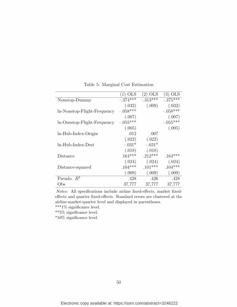
Electronic copy available at: https://ssrn.com/abstract=3246222
Table 5: Marginal Cost Estimation
(1) OLS (2) OLS (3) OLSNonstop-Dummy –.374*** –.313*** –.375***
(.032) (.009) (.032)ln-Nonstop-Flight-Frequency –.058*** –.058***
(.007) (.007)ln-Onestop-Flight-Frequency –.055*** –.055***
(.005) (.005)ln-Hub-Index-Origin .012 .007
(.022) (.022)ln-Hub-Index-Dest –.031* –.031*
(.018) (.018)Distance .164*** .212*** .164***
(.024) (.024) (.024)Distance-squared .104*** .101*** .104***
(.009) (.009) (.009)Pseudo. R2 .428 .426 .428Obs 37,777 37,777 37,777
Notes: All specifications include airline fixed-effects, market fixed-effects and quarter fixed-effects. Standard errors are clustered at theairline-market-quarter level and displayed in parentheses.***1% significance level.**5% significance level.*10% significance level.
50

Electronic copy available at: https://ssrn.com/abstract=3246222
flight frequency by one reduces marginal cost of serving one-stop passengers by $0.60.
Cost of serving passengers is also lower if any endpoint is a hub airport.
6.4 Stage 2: Estimation of Marginal Cost of Building Fre-
quencies
I use estimates in Table 4 and Table 5 to calculate the marginal variable profit asso-
ciated with an additional nonstop flight frequency in all markets.
Figure 2: Decomposition of Marginal Variable Profit
Figure 2 decomposes and summarizes the marginal variable profit from an extra
flight. The first row reports marginal variable profit from additional nonstop service.
The second row reports its cannibalization effect on existing one-stop services. The
third row reports marginal variable profit from additional one-stop service. The forth
row reports its cannibalization effect on existing nonstop service. The last row reports
the total marginal variable profit associated with an additional flight, which sums
51

Electronic copy available at: https://ssrn.com/abstract=3246222
Table 6: Decomposition of Marginal Variable Profits for an Additional Flight (in$100’s)
Variable Mean Std. Dev.∆π from Additional Nonstop Service 67.476 99.737Cannibalization from One-stop Services -2.562 10.472∆π from Additional One-stop 11.304 22.346Cannibalization from Nonstop Services -0.682 2.067Total ∆π 75.536 105.099
Obs. 6934
up the first four rows. According to marginal cost optimality for flight frequency,
this total marginal variable profit should equal the marginal cost of scheduling an
additional flight.
On average, if an airline schedules an extra flight, it can bring in marginal variable
profit of $6747 from nonstop service and $1130 from one-stop service. The average
marginal cost of scheduling flight frequency is equal to $7554. This value is consistent
with the industry measure of flight operation cost. So if ignoring airline network
structure would underestimate the costs and benefits of an additional flight frequency
by 11%.
Table 7 reports the estimates of the marginal cost of flight frequency. The re-
lationship between distance and marginal cost resembles an inverted U-shape. The
marginal cost of flight frequency in a market is higher when an endpoint of this mar-
ket has a higher hub index. According to the estimates of demand and the marginal
cost of serving passengers, higher hub indexes in a market result in higher demand
and lower cost of serving passengers. Airlines that schedule more flights in their hub
city suffer from higher cost of scheduling an additional flight due to congestion or
capacity constraints.43
43In this paper, I assume that the marginal cost of scheduling flight frequency is not a function offlight frequency. This assumption may be relaxed later.
52

Electronic copy available at: https://ssrn.com/abstract=3246222
Table 7: Estimation Result: Marginal Cost of Building Flight Frequency
(1)MCFF
ln-Hub-Index-Origin .248***(.020)
ln-Hub-Index-Dest .169***(.015)
Distance 2.335***(.017)
Distance-squared –.514***(.007)
Pseudo. R2 .984Obs 6934
Notes: All specifications includeairline-city fixed-effects and quar-ter fixed-effects. Standard errorsare clustered at the airline-market-quarter level and displayed in paren-theses.***1% significance level.**5% significance level.*10% significance level.
6.5 Stage 3: Estimation of Entry Cost
Empirically, I find that B∗ = 170 optimizes model fit in fixed cost estimation. Table
8 reports entry cost estimates for the year 2014 when B = B∗ = 170. Section 6.6
further discusses model goodness of fit.
When gate share at the two endpoints increases by 1 percent, entry cost decreases
by $0.22 million a quarter. So an airline that dominates an airport faces lower entry
cost into markets connected to this airport. Legacy carriers control a greater pro-
portion of gates compared to low cost carriers, which reduces their entry cost and
facilitates their entry decisions and operations. I conclude that gate ownership at
airports is an important element of airline operations and competition. There is het-
erogeneity in entry cost across airlines. The difference in entry cost among the legacy
53

Electronic copy available at: https://ssrn.com/abstract=3246222
Table 8: Entry Cost (in Millions $ a Quarter)
Characteristics Estimates
Gate -22.83[-23.28,-22.32]
Quarter Estimates
Q1 (Omitted)-
Q2 1.84[0.66,2.49]
Q3 -0.75[-1.62,-0.36]
Q4 -1.06[-1.33,0.23]
Airline Estimates
WN (Southwest Airlines) 3.67[2.16,5.06]
DL (Delta Air Lines) -0.05[-0.85,5.62]
AA (American Airlines) (Omitted)-
UA (United Airlines) 0.90[-2.07,1.38]
B6 (JetBlue Airways) 0.20[-5.17,3.16]
F9 (Frontier Airlines) -1.13[-6.07,-0.32]
AS (Alaska Airlines) -1.26[-2.99,0.18]
NK (Spirit Airlines) -0.68[-2.82,5.38]
VX (Virgin America) -1.64[-3.49,-0.23]
Obs 21459
Notes: 95% confidence intervals are displayedin parentheses. Confidence intervals are con-structed from 500 group samplings.
54
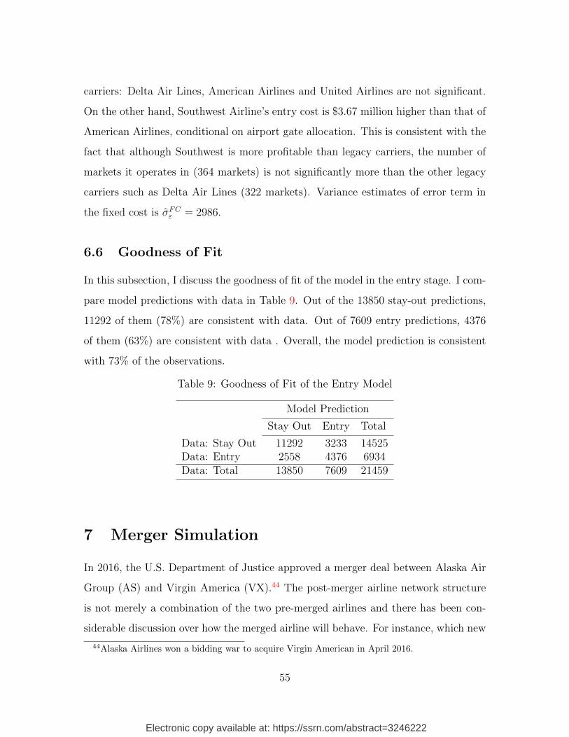
Electronic copy available at: https://ssrn.com/abstract=3246222
carriers: Delta Air Lines, American Airlines and United Airlines are not significant.
On the other hand, Southwest Airline’s entry cost is $3.67 million higher than that of
American Airlines, conditional on airport gate allocation. This is consistent with the
fact that although Southwest is more profitable than legacy carriers, the number of
markets it operates in (364 markets) is not significantly more than the other legacy
carriers such as Delta Air Lines (322 markets). Variance estimates of error term in
the fixed cost is σFCε = 2986.
6.6 Goodness of Fit
In this subsection, I discuss the goodness of fit of the model in the entry stage. I com-
pare model predictions with data in Table 9. Out of the 13850 stay-out predictions,
11292 of them (78%) are consistent with data. Out of 7609 entry predictions, 4376
of them (63%) are consistent with data . Overall, the model prediction is consistent
with 73% of the observations.
Table 9: Goodness of Fit of the Entry Model
Model Prediction
Stay Out Entry Total
Data: Stay Out 11292 3233 14525Data: Entry 2558 4376 6934Data: Total 13850 7609 21459
7 Merger Simulation
In 2016, the U.S. Department of Justice approved a merger deal between Alaska Air
Group (AS) and Virgin America (VX).44 The post-merger airline network structure
is not merely a combination of the two pre-merged airlines and there has been con-
siderable discussion over how the merged airline will behave. For instance, which new
44Alaska Airlines won a bidding war to acquire Virgin American in April 2016.
55

Electronic copy available at: https://ssrn.com/abstract=3246222
markets will the new post-merger airline enter? How will this post-merger airline
re-allocate its flights? How will other airlines respond? How will prices and consumer
surplus change in the markets previously served by Alaska or Virgin American or
even markets that were not served by the two airlines pre-merger? These interesting
questions cannot be answered with existing models which treat network structures
as exogenously given. In this counterfactual study, I investigate the consequences of
an exogenous merger between the two airlines. This paper focuses on examining the
extent to which the merger affects the network structures of all airlines; airline merger
incentives are not explored.
7.1 Merger Simulation Set-up
Pre-Merger Network Set-up
To simulate a pre-merger network structure, I assume the values of primitives of the
model are the same as their estimates.45 Airlines will maintain their gate allocations
at each airport. Specifically, I draw fixed cost from a normal distribution, using the
fitted fixed cost estimate and its standard error as the mean and standard deviation,
respectively, i.e., FCsimunijt ∼ N(γFCG (Gnit +Gnjt) + ηFCn + ηFCt + ηFCi + ηFCj , σFCε ).
Post-Merger Network Set-up
To simulate the post-merger network structure, I assume that non-merging airlines
maintain their gate allocations and unobserved product quality in consumer demand,
marginal cost, and flight frequency. Merging airlines are eliminated post-merger and
replaced with a new airline. The post-merger airline owns all gates from the merging
airlines.46 Post-merger unobserved product quality in demand and cost are calculated
as the weighted average of the merging airlines. For markets in which both Alaska
45The primitives of the model include consumer utility functions, variable costs of serving passen-gers and of increasing flight frequency, and fixed cost.
46In reality, there may be some gate or slot reallocation post-merger; for simplicity, I assume thereis no change in gate allocations.
56

Electronic copy available at: https://ssrn.com/abstract=3246222
Airlines and Virgin America were active pre-merger, I determine these weights based
on the merging companies’ relative flight frequencies. For markets in which neither
Alaska Airlines nor Virgin America were active pre-merger, I calculate weights based
on their gates shares at the two endpoints.
7.2 Algorithm to Simulate An Equilibrium
Sequence of Moves
Since it is computationally infeasible to obtain a Nash equilibrium of this simultaneous-
move network competition game, I reconstruct this simultaneous game as a sequential-
move game. I propose a sequence by which all airline-market pairs move. Airlines
first move in larger markets, then move in smaller markets. Within each market,
airlines move sequentially by profitability.47 For instance, New York - Los Angeles
is the largest market, in which JetBlue is the most profitable airline and American
Airline is the second most profitable airline. My proposed sequence would therefore
assign JetBlue and American Airline as the first and second movers, respectively, in
the NY-LA market, followed by other airlines in descending market profitability or-
der. After these airlines in the largest market have moved, the sequence moves on to
airlines in the second largest market New York - Chicago. Again, airlines with higher
profitability move first, followed by airlines with lower profitability. In this way, I
obtain a sequence of all airline-market pairs.
For this massive sequential move game, I should ideally solve for the sub-game
perfect Nash equilibrium using backward induction. However, since it is impossible
to compute the profit of the airlines at all branches of the game tree, I use a forward
induction algorithm to search for an equilibrium.
Starting with an empty network where no airlines are active in any market, I
evaluate airline best response, airline-market pair by airline-market pair according to
47Berry (1992) estimates a model of sequential market entry of the airlines. He orders airlinesaccording to profitability and incumbency status of the airlines.
57

Electronic copy available at: https://ssrn.com/abstract=3246222
the sequence defined above. Specifically, starting with the first airline-market pair
in the sequence, I evaluate the best response of this airline in that specific market.48
I update airline network structures each time an airline enters, exits, or changes
flight frequency in a market. Then, I proceed to the second airline-market pair in
the sequence, evaluate the best response of this airline in the market and update its
network structure. After all airline-market pairs are visited, I go back to the first
airline-market pair and re-evaluate the best responses of the entire airline-market
sequence. If there is no incentive to deviate, this convergence of best responses in the
network serves as an approximation of the subgame perfect Nash equilibrium of the
sequential-move game.49
Airline Best Response
This subsection describes how I derive the best responses of the airlines. When airline
n determines its optimal entry decision and flight frequency for a given market, it
treats as given not only its own entry and flight frequency decisions in other markets
but also other airlines’ entry and flight frequency decisions in all markets. Since there
is no explicit solution for the optimal entry decision and flight frequency, I numerically
calculate the profit of each airline associated with all possible flight frequencies in this
market. For any possible flight frequency of an airline in a market, I first simulate
the counterfactual network structure of this airline to determine the Bertrand Nash
equilibrium in prices for all markets, which I use to calculate the overall profit of
the airline associated with the given flight frequency. The airline will schedule its
flights to maximize its overall profit. To reduce computation burden, I also restrict
the choice set of the airlines. In any market, an airline has 6 possible options: it can
out of the market, or it can enter this market and offer (2,4,6,8,10) daily flights.
48I will discuss how to compute the best response of the airline in the next subsection.49In the robustness check, I consider other sequences of airline-market where the order of all
airline-market pairs is randomized.
58

Electronic copy available at: https://ssrn.com/abstract=3246222
7.3 Counterfactual Results
For this policy experiment, I draw 10 different sets of fixed costs, simulate both
benchmark network structure and counterfactual network structures, and report the
average of the 10 simulations.50
Table 10 and Table 11 compare the market structures of benchmark networks
versus counterfactual networks. In both tables, the first three rows summarize airlines’
nonstop networks (number of nonstop markets, number of nonstop flight frequencies,
and revenue from nonstop services), the fourth to the sixth rows summarize airlines’
one-stop networks (number of one-stop markets, number of one-stop flight frequencies,
and revenue from one-stop services) and the last row summarizes the variable profit
of the airlines.
In Table 10, the first two columns report the simulated benchmark networks of
Alaska Airline and Virgin America, respectively. Averaged across all simulations,
Alaska Airline operates nonstop service in 258 markets, which are six times the non-
stop markets of Virgin America pre-merger. Virgin America does not operate one-stop
service while Alaska operates one-stop flights in 52 markets. The third column reports
the counterfactual network of the new post-merger airline. The post-merger airline
will operate nonstop service in 291 markets and offer increased flight frequency (2302
daily flights) greater than the pre-merger offerings (1722+188=1910 daily flights).
The post-merger airline will operate in more one-stop markets because it now has a
larger network, which can facilitate its one-stop operations. In terms of revenue, the
post-merger airline will bring in more variable profit compared to the two pre-merger
airlines. On average, the post-merger airline will enter 32 nonstop markets and 1
one-stop markets but exit 13 nonstop markets.
Table 11 summarizes the network structures of all the other airlines before and af-
50It takes approximately one day for one iteration to converge using an Intel i7 8-core, 16G RAMcomputer. The network converges in 3-6 iterations. The detailed network structure of each set offixed costs can be found in the online appendix.
59

Electronic copy available at: https://ssrn.com/abstract=3246222
Table 10: Counterfactual Results: Network Structures of AS and VX
Benchmark CT Change
AS VX AS + VX Entry Exit
NonstopaNS 258 42 291 32 13fNS 1722 188 2302 294 50RevNS 9999 2680 19325 7497 10
One-stopaOS 52 0 53 1 0fOS 105 0 132 0 0RevOS 2080 0 1248 0 0
Variable Profitπ 11371 2066 18580
Note: revenue and profit are measured by million dollars in a quarter.
ter the AS-VX merger.51 The first column reports the simulated benchmark network.
Other airlines operate nonstop service in 8953 markets with 78064 daily flights and
earn $253 billion dollars in a quarter. They also operate one-stop service in 6012 mar-
kets. Revenues from nonstop service are about three times that of one-stop service.
The second column summarizes counterfactual networks of the other airlines and the
third and fourth columns report entries and exits of the other airlines, respectively.
Following the AS-VX merger, the other airlines are projected to slightly expand their
operations, entering into 3 nonstop markets and exiting from 1 nonstop market.
Table 12 reports change in consumer surplus and number of entries and exits
by market size. The first two columns report entries and exits of the airlines and
the last three columns report change in welfare. The first four rows report different
quantiles of markets and the last row reports the sum. In larger markets, there
are more entries than exits, resulting in net entries.52 In contrast, there are no
entries in smaller markets and consumer welfare may slightly reduce in these markets.
Overall, consumer surplus increases by 1.28% with consumer surplus in larger markets
51Other airlines refer to all airlines except Alaska and Virgin America.52The identity of the airlines that operate in these markets may be different.
60

Electronic copy available at: https://ssrn.com/abstract=3246222
Table 11: Counterfactual Results: Network Structures of other airlines
Benchmark CT Change
Other Air Other Air Entry Exit
NonstopaNS 8953 8955 3 1fNS 78064 78064 110 20RevNS 253098 281878 131 28
One-stopaOS 6012 6012 0 0fOS 26980 26963 0 0RevOS 109596 132410 0 0
Variable Profitπ 346273 397955
Note: Revenue and profit are measured by million dollars in a quarter.
increasing more compared to the consumer surplus in smaller markets.
Table 12: Counterfactual Results: Welfare Analysis
Market Size Market Entries and Exits Change in Welfare (Million $)
Quartile Entry Exit Benchmark CT Change(%)
1 29 12 542857 555450 2.320
2 4 2 284280 285338 0.372
3 2 0 165476 165824 0.210
4 0 0 99883 99882 -0.001
Total 35 14 1092495 1106494 1.281
Note: Consumer surplus is measured by million dollars in a quarter.
8 Conclusion
This paper proposes and estimates one of the first models of airline network com-
petition to endogenize network structure, flight frequencies, prices and quantities for
61

Electronic copy available at: https://ssrn.com/abstract=3246222
every nonstop and one-stop market. Since solving for an equilibrium is computa-
tionally infeasible, I estimate cost of increasing flight frequencies by making use of
the marginal condition of optimality and infer entry cost by exploiting inequality
restrictions implied by airlines’ revealed preferences.
I use this model to study the effect of marginal costs, entry costs, variable profits
and strategic interactions in both nonstop and one-stop services in airline network
competition. I find that synergies across markets are crucial to determining airline
entry decisions. Airlines construct their network structures and schedule their flights
strategically to provide one-stop service to consumers. Ignoring one-stop products
could therefore result in underestimating the marginal cost of flight frequency by
up to 11%. The paper further applies the proposed methodology to predict the
consequences of a hypothetical merger between Alaska Airlines and Virgin America in
the first quarter of 2014. This counterfactual simulation predicts that the new post-
merger airline would re-optimize its network structure, enter 32 nonstop markets,
and exit 13 nonstop markets. The merger is expected to improve consumer welfare
overall through increased airline entry, with welfare increasing in larger markets and
decreasing in smaller markets.
References
Aguirregabiria, V., R. Clark, and H. Wang (2016): “Diversification of ge-
ographic risk in retail bank networks: evidence from bank expansion after the
Riegle-Neal Act,” The RAND Journal of Economics, 47(3), 529–572.
Aguirregabiria, V., and C.-Y. Ho (2012): “A dynamic oligopoly game of the
US airline industry: estimation and policy experiments,” Journal of Econometrics,
168(1), 156–173.
Andrews, D. W., and X. Shi (2013): “Inference based on conditional moment
inequalities,” Econometrica, 81(2), 609–666.
62

Electronic copy available at: https://ssrn.com/abstract=3246222
Benkard, C. L., A. Bodoh-Creed, and J. Lazarev (2010): “Simulating the
dynamic effects of horizontal mergers: US airlines,” Manuscript, Yale University.
Berry, S., M. Carnall, and P. T. Spiller (2006): “Airline hubs: costs, markups
and the implications of customer heterogeneity,” In: Lee, D. (Ed.), Advances in
Airline Economics. Vol. 1: Competition Policy and Antitrust. Elsevier Press, Am-
sterdam, pp. 183–214.
Berry, S., J. Levinsohn, and A. Pakes (1995): “Automobile prices in market
equilibrium,” Econometrica: Journal of the Econometric Society, pp. 841–890.
Berry, S, S., and P. Jia, P. (2010): “Tracing the woes: an empirical analysis of
the airline industry,” American economic journal. Microeconomics, 2(3), 1–43.
Berry, S. T. (1990): “Airport presence as product differentiation,” The American
Economic Review, pp. 394–399.
(1992): “Estimation of a model of entry in the airline industry,” Economet-
rica: Journal of the Econometric Society, pp. 889–917.
(1994): “Estimating discrete-choice models of product differentiation,” The
RAND Journal of Economics, pp. 242–262.
Blevins, J. R. (2015): “Structural estimation of sequential games of complete in-
formation,” Economic Inquiry, 53(2), 791–811.
Borenstein, S. (1989): “Hubs and high fares: dominance and market power in the
US airline industry,” The RAND Journal of Economics, pp. 344–365.
Brueckner, J. K., and P. T. Spiller (1994): “Economies of traffic density in
the deregulated airline industry,” Journal of Law and Economics, pp. 379–415.
Chernozhukov, V., H. Hong, and E. Tamer (2007): “Estimation and confidence
regions for parameter sets in econometric models,” Econometrica, 75(5), 1243–1284.
63

Electronic copy available at: https://ssrn.com/abstract=3246222
Ciliberto, F., E. Cook, and J. Williams (2018): “Network Structure and Con-
solidation in the US Airline Industry, 1990-2015,” .
Ciliberto, F., C. Murry, and E. T. Tamer (2016): “Market structure and
competition in airline markets,” .
Ciliberto, F., and E. Tamer (2009): “Market structure and multiple equilibria
in airline markets,” Econometrica, 77(6), 1791–1828.
Ciliberto, F., and J. W. Williams (2010): “Limited access to airport facilities
and market power in the airline industry,” Journal of Law and Economics, 53(3),
467–495.
(2014): “Does multimarket contact facilitate tacit collusion? Inference on
conduct parameters in the airline industry,” The RAND Journal of Economics,
45(4), 764–791.
Ciliberto, F., and Z. Zhang (2014): “Multiple equilibria and deterrence in airline
markets,” Manuscript, University of Virginia.
Dou, L., J. Lazarev, and J. Kastl (2017): “Quantifying Delay Externalities in
Airline Networks,” Working Paper.
Ellickson, P. B., S. Houghton, and C. Timmins (2013): “Estimating network
economies in retail chains: a revealed preference approach,” The RAND Journal of
Economics, 44(2), 169–193.
Fan, Y. (2013): “Ownership consolidation and product characteristics: a study of the
US daily newspaper market,” The American Economic Review, 103(5), 1598–1628.
Gayle, P. G., and J. O. Yimga (2015): “Airline alliance and product quality: the
case of the US domestic airline industry,” Working paper.
64

Electronic copy available at: https://ssrn.com/abstract=3246222
Gedge, C., J. W. Roberts, and A. Sweeting (2017): “A model of dynamic limit
pricing with an application to the airline industry,” Discussion paper, National
Bureau of Economic Research.
Hendricks, K., M. Piccione, and G. Tan (1997): “Entry and exit in hub-spoke
networks,” The RAND Journal of Economics, pp. 291–303.
(1999): “Equilibria in networks,” Econometrica, 67(6), 1407–1434.
Jia, P. (2008): “What happens when wal-mart comes to town: an empirical analysis
of the discount retailing industry,” Econometrica, 76(6), 1263–1316.
Kundu, C. (2014): “Essays in empirical industrial organization of US domestic
airline industry,” Ph.D. thesis, The Ohio State University.
Lazarev, J. (2013): “The welfare effects of intertemporal price discrimination: an
empirical analysis of airline pricing in US monopoly markets,” Working Paper.
Li, S. Y., J. Mazur, Y. Park, J. W. Roberts, A. Sweeting, and J. Zhang
(2018): “Endogenous and Selective Service Choices After Airline Mergers,” .
Molnar, A. (2013): “Congesting the commons: A test for strategic congestion
externalities in the airline industry,” Working Paper.
Nevo, A. (2000): “Mergers with differentiated products: The case of the ready-to-
eat cereal industry,” The RAND Journal of Economics, pp. 395–421.
Nishida, M. (2014): “Estimating a model of strategic network choice: The
convenience-store industry in Okinawa,” Marketing Science, 34(1), 20–38.
Onishi, Y., and Y. Omori (2014): “Bayesian estimation of entry games with mul-
tiple players and multiple equilibria,” Working Paper.
Pakes, A., J. Porter, K. Ho, and J. Ishii (2015): “Moment Inequalities and
Their Application,” Econometrica, 83(CWP16/07), 315–334.
65

Electronic copy available at: https://ssrn.com/abstract=3246222
Peters, C. (2006): “Evaluating the performance of merger simulation: Evidence
from the US airline industry,” The Journal of law and economics, 49(2), 627–649.
Richard, O. (2003): “Flight frequency and mergers in airline markets,” Interna-
tional Journal of Industrial Organization, 21(6), 907–922.
Seim, K. (2006): “An empirical model of firm entry with endogenous product-type
choices,” The RAND Journal of Economics, 37(3), 619–640.
Snider, C. (2009): “Predatory incentives and predation policy: the American Air-
lines case,” Manuscript. Department of Economics. UCLA.
Sweeting, A. (2013): “Dynamic product positioning in differentiated product mar-
kets: the effect of fees for musical performance rights on the commercial radio
industry,” Econometrica, 81(5), 1763–1803.
Williams, J. W. (2008): “Capacity investments, exclusionary behavior, and welfare:
a dynamic model of competition in the airline industry,” Exclusionary Behavior,
and Welfare: A Dynamic Model of Competition in the Airline Industry (December
1, 2008).
Williams, K. R. (2017): “Dynamic airline pricing and seat availability,” .
Zhu, T., and V. Singh (2009): “Spatial competition with endogenous location
choices: an application to discount retailing,” Quantitative Marketing and Eco-
nomics, 7(1), 1–35.
66

Electronic copy available at: https://ssrn.com/abstract=3246222
A Bankruptcies and Mergers
Some airline bankruptcies and mergers take place during the sample period. I con-
sider four major mergers: Delta announced a merger with Northwest on Apr. 14th,
2008, completing the transaction on Dec. 31st, 2009; United Airlines merged with
Continental on May. 3rd, 2010, with a closing day of Oct. 1st, 2010; Southwest
controlled AirTran’s assets after AirTran’s bankruptcy on Sep. 27th, 2010. AMR
Corporation, the former parent company of American Airlines, completed the merger
with US Airways Group on December 9, 2013. For the analysis, two merging airlines
are treated as the same airline after closing day but as different airlines before closing
day. Given this, Northwest disappears in 2010 Q1; Continental flights are considered
United Airlines flights after 2010 Q4; very few AirTran tickets in 2008 Q2 are consid-
ered to be Southwest tickets and US Airway tickets and operations are considered to
be a part of American Airlines after 2014Q1.
B Computation of Consumer Welfare
Consumer welfare is computed according to the following formula
W = σ1ln[∑G
(∑g
exp(Vg,G))σ2σ1 ], (51)
where Vi is the deterministic component of the indirect utility function.
67