Near Neighbor JoinHerald Kllapi #+1, Boulos Harb ∗2, Cong Yu ∗3

# Dept. of Informatics and Telecommunications, University of AthensPanepistimiopolis, Ilissia Athens 15784, Greece

1 herald@di.uoa.gr+Work done while at Google Research.

∗ Google Research,75 Ninth Avenue, New York, NY 10011, USA

2 harb@google.com3 congyu@google.com

Abstract—An increasing number of Web applications such asfriends recommendation depend on the ability to join objects atscale. The traditional approach taken is nearest neighbor join(also called similarity join), whose goal is to find, based on agiven join function, the closest set of objects or all the objectswithin a distance threshold to each object in the input. Thescalability of techniques utilizing this approach often depends onthe characteristics of the objects and the join function. However,many real-world join functions are intricately engineered andconstantly evolving, which makes the design of white-box methodsthat rely on understanding the join function impractical. Findinga technique that can join extremely large number of objects withcomplex join functions has always been a tough challenge.

In this paper, we propose a practical alternative approachcalled near neighbor join that, although does not find the closestneighbors, finds close neighbors, and can do so at extremelylarge scale when the join functions are complex. In particular, wedesign and implement a super-scalable system we name SAJ thatis capable of best-effort joining of billions of objects for complexfunctions. Extensive experimental analysis over real-world largedatasets shows that SAJ is scalable and generates good results.

I. INTRODUCTION

Join has become one of the most important operationsfor Web applications. For example, to provide users withrecommendations, social networking sites routinely comparethe behaviors of hundreds of millions of users [1] to identify,for each user, a set of similar users. Further, in many searchapplications (e.g., [2]), it is often desirable to showcaseadditional results among billions of candidates that are relatedto those already returned.

The join functions at the core of these applications are oftenvery complex: they go beyond the database style θ-joins or theset-similarity style joins. For example, in Google Places, thesimilarity of two places are computed based on combinationsof spatial features and content features. For WebTables usedin Table Search [3], the similarity function employs a multi-kernel SVM machine learning algorithm. Neither function iseasy to analyze.

Furthermore, the needs of such applications change andthe join functions are constantly evolving, which makes itimpractical to use a system that heavily depends on function-specific optimizations. This complex nature of real-world joinfunctions makes the join operation especially challenging to

perform at large scale due to its inherently quadratic nature,i.e., there is no easy way to partition the objects such that onlyobjects within the same partition need to be compared.

Fortunately, unlike database joins where exact answers arerequired, many Web applications accept join results as longas they are near. For a given object, missing some or evenall of the objects that are nearest to it, is often tolerable ifthe objects being returned are almost as near to it as thosethat are nearest. Inability to scale to the amount of data thoseapplications must process, however, is not an option. In fact, akey objective for all such applications is to balance the resultaccuracy and the available machine resources while processingthe data in its entirety.

In this paper, we introduce SAJ1, a Scalable ApproximateJoin system that performs near neighbor join of billionsof objects of any type with a broader set of complex joinfunctions, where the only expectation on the join function isthat it satisfies the triangle inequality2. More specifically, SAJaims to solve the following problem: Given (1) a set I of Nobjects of type T , where N can be billions; (2) a complexjoin function FJ : T ×T → R that takes two objects in I andreturns their similarity; and (3) resource constraints (specifiedas machine per-task computation capacity and number ofmachines). For all o ∈ I , find k objects in I that are similar too according to FJ without violating the machine constraints.

As with many other recent parallel computation systems,SAJ adopts the MapReduce programming model [4]. At a highlevel, SAJ operates in two distinct multi-iteration phases. Inthe initial Bottom-Up (BU) phase, the set of input objects areiteratively partitioned and clustered within each partition toproduce a successively smaller set of representatives. Eachrepresentative is associated with a set of objects that aresimilar to it within the partitions in the previous iteration.In the following Top-Down (TD) phase, at each iteration themost similar pairs of representatives are selected to guide thecomparison of objects they represent in the upcoming iteration.

1In Arabic, Saj is a form of rhymed prose known for its evenness, acharacteristic that our system strives for.

2In fact, even the triangle inequality of the join function is not a strictrequirement within SAJ, it is only needed if a certain level of quality is to beexpected, see Section V.

To achieve true scalability, SAJ respects the resource con-straints in two critical aspects. First, SAJ strictly adheres tomachine per-task capacity by controlling the partition sizeso that it is never larger than the number of objects eachmachine can handle. Second, SAJ allows developers duringthe TD phase to easily adjust the accuracy requirements inorder to satisfy the resource constraint dictated by the numberof machines. Because of these design principles, in one ofour scalability experiments, SAJ completed a near-k (wherek = 20) join for 1 billion objects within 20 hours.

To the best of our knowledge, our system is the first attemptat super large scale join without detailed knowledge of the joinfunction. Our specific contributions are:• We propose a novel top-down scalable algorithm for se-lectively comparing promising object pairs starting with asmall set of representative objects that are chosen based onwell-known theoretical work.• Based on the top-down approach, we build an end-to-endjoin system capable of processing near neighbor joins overbillions of objects without requiring detailed knowledgeabout the join function.• We provide algorithmic analysis to illustrate how oursystem scales while conforming to the resource constraints,and theoretical analysis of the quality expectation.• We conducted extensive experimental analysis over largescale datasets to demonstrate the system’s scalability.The rest of the paper is organized as follows. Section II

presents the related work. Section III introduces the basicterminologies we use, the formal problem definition, and anoverview of the SAJ system. Section IV describes the tech-nical components of SAJ. Analysis of the algorithms and theexperiments are described in Sections V and VI, respectively.Finally, we conclude in Section VII.

II. RELATED WORK

Similarity join has been studied extensively in recent lit-erature. The work by Okcan and Riedewald [5] describesa cost model for analyzing database-style θ-joins, based onwhich an optimal join plan can be selected. The work byVernica et. al. [6] is one of the first to propose a MapReduce-based framework for joining large data sets using set similarityfunctions. Their approach is to leverage the nature of set sim-ilarity functions to prune away a large number of pairs beforethe remaining pairs are compared in the final reduce phase.More recently, Lu et. al. [7] apply similar pruning techniquesto joining objects in n-dimensional spaces using MapReduce.Similar to [6], [7], there are a number of studies on scalablesimilarity join using parallel and/or p2p techniques [8], [9],[10], [7], [11], [12], [13], [14]. Those proposed techniques dealwith join functions in two main categories: (i) set similaritystyle joins where the objects are represented as sets (e.g.,Jaccard), or (ii) join functions that are designed for spatialobjects in n-dimensional vector space, such as Lp distance.

Our work distinguishes itself in three main aspects. First, allprior works use knowledge about the join function to performpruning and provide exact results. SAJ, while assuming triangle

inequality for improved result quality, assumes little aboutthe join function and produces best-effort results. Second,objects in those prior works must be represented either asa set or a multi-dimensional point, while SAJ makes noassumption about how object can be represented. Third, thescalability of some of these studies follows from adopting ahigh similarity threshold, hence they cannot guarantee that kneighbors are found for every object. The tradeoff is that SAJonly provides best-effort results, which are reasonable for realworld applications that require true scalability and can toleratenon-optimality.

Scalable (exact and approximate) similarity joins for knownjoin functions have been studied extensively in non-parallelcontexts [15], [16], [17], [18], [19], [20], [21], [22], [23],[24], [25]. The join functions being considered include editdistance, set similarity, cosine similarity, and Lp distance.Again, they all use knowledge about the join functions toprune candidate pairs and avoid unnecessary comparisons.For general similarity join, [26] introduces a partition basedjoin algorithm that only requires the join function to havethe metric property. The algorithm, however, is designed todiscover object pairs within ε distance of each other instead offinding k neighbors of each object. LSH has been effective forboth similarity search [27] and similarity join [28]; however,it is often difficult to find the right hash functions.

There are some works that consider the problem of incre-mental kNN join [29]. Since our framework is implementedon top of MapReduce, we focus on designing a system thatscales to billions of objects using batch processing of read-only datasets and do not consider this case.

Our work is related to techniques developed for kNNsearch [30], whose hashing techniques can potentially beleveraged in SAJ. Also focusing on search, there are severalworks that use a similar notion of representative objects tobuild a tree and prune the search space based on the triangleinnequality property [31], [32], [33]. Finally, our Bottom-Upalgorithm adopts the streaming clustering work in [34].

III. PRELIMINARIES & SAJ OVERVIEW

Notation SemanticsI,N = |I| The set of input objects and its size

k Desired number of near neighbors per objectn Maximum number of objects a machine

can manipulate in a single task, n� Nm Number of clusters per local partition, m < nP Number of top object pairs maintained for

each TD iteration, P � N2

p Maximum number of object pairs sent to amachine in each TopP iteration, p > P

FJ Required user-provided join function:FJ : I × I → R

FP Optional partition function: FP : I → stringFR Optional pair ranking function:

FR : (I, I)× (I, I)→ R

TABLE IADOPTED NOTATION.

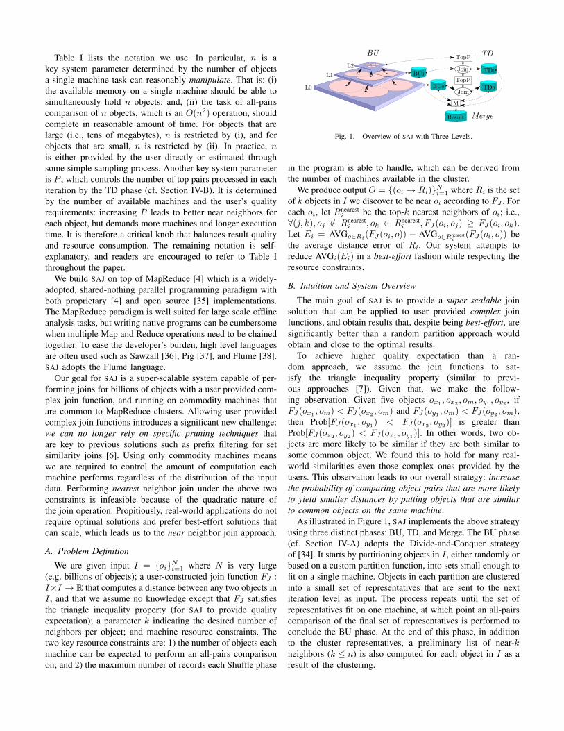
Table I lists the notation we use. In particular, n is akey system parameter determined by the number of objectsa single machine task can reasonably manipulate. That is: (i)the available memory on a single machine should be able tosimultaneously hold n objects; and, (ii) the task of all-pairscomparison of n objects, which is an O(n2) operation, shouldcomplete in reasonable amount of time. For objects that arelarge (i.e., tens of megabytes), n is restricted by (i), and forobjects that are small, n is restricted by (ii). In practice, nis either provided by the user directly or estimated throughsome simple sampling process. Another key system parameteris P , which controls the number of top pairs processed in eachiteration by the TD phase (cf. Section IV-B). It is determinedby the number of available machines and the user’s qualityrequirements: increasing P leads to better near neighbors foreach object, but demands more machines and longer executiontime. It is therefore a critical knob that balances result qualityand resource consumption. The remaining notation is self-explanatory, and readers are encouraged to refer to Table Ithroughout the paper.

We build SAJ on top of MapReduce [4] which is a widely-adopted, shared-nothing parallel programming paradigm withboth proprietary [4] and open source [35] implementations.The MapReduce paradigm is well suited for large scale offlineanalysis tasks, but writing native programs can be cumbersomewhen multiple Map and Reduce operations need to be chainedtogether. To ease the developer’s burden, high level languagesare often used such as Sawzall [36], Pig [37], and Flume [38].SAJ adopts the Flume language.

Our goal for SAJ is a super-scalable system capable of per-forming joins for billions of objects with a user provided com-plex join function, and running on commodity machines thatare common to MapReduce clusters. Allowing user providedcomplex join functions introduces a significant new challenge:we can no longer rely on specific pruning techniques thatare key to previous solutions such as prefix filtering for setsimilarity joins [6]. Using only commodity machines meanswe are required to control the amount of computation eachmachine performs regardless of the distribution of the inputdata. Performing nearest neighbor join under the above twoconstraints is infeasible because of the quadratic nature ofthe join operation. Propitiously, real-world applications do notrequire optimal solutions and prefer best-effort solutions thatcan scale, which leads us to the near neighbor join approach.

A. Problem Definition

We are given input I = {oi}Ni=1 where N is very large(e.g. billions of objects); a user-constructed join function FJ :I×I → R that computes a distance between any two objects inI , and that we assume no knowledge except that FJ satisfiesthe triangle inequality property (for SAJ to provide qualityexpectation); a parameter k indicating the desired number ofneighbors per object; and machine resource constraints. Thetwo key resource constraints are: 1) the number of objects eachmachine can be expected to perform an all-pairs comparisonon; and 2) the maximum number of records each Shuffle phase

L0

L1

L2

BU0

BU1

TD0

TD1

TopP

TopP

Join

Join

M

Result

BU TD

Merge

Fig. 1. Overview of SAJ with Three Levels.

in the program is able to handle, which can be derived fromthe number of machines available in the cluster.

We produce output O = {(oi → Ri)}Ni=1 where Ri is the setof k objects in I we discover to be near oi according to FJ . Foreach oi, let Rnearest

i be the top-k nearest neighbors of oi; i.e.,∀(j, k), oj /∈ Rnearest

i , ok ∈ Rnearesti , FJ(oi, oj) ≥ FJ(oi, ok).

Let Ei = AVGo∈Ri(FJ(oi, o)) − AVGo∈Rnearesti

(FJ(oi, o)) bethe average distance error of Ri. Our system attempts toreduce AVGi(Ei) in a best-effort fashion while respecting theresource constraints.

B. Intuition and System Overview

The main goal of SAJ is to provide a super scalable joinsolution that can be applied to user provided complex joinfunctions, and obtain results that, despite being best-effort, aresignificantly better than a random partition approach wouldobtain and close to the optimal results.

To achieve higher quality expectation than a ran-dom approach, we assume the join functions to sat-isfy the triangle inequality property (similar to previ-ous approaches [7]). Given that, we make the follow-ing observation. Given five objects ox1

, ox2, om, oy1

, oy2, if

FJ(ox1, om) < FJ(ox2

, om) and FJ(oy1, om) < FJ(oy2

, om),then Prob[FJ(ox1

, oy1) < FJ(ox2

, oy2)] is greater than

Prob[FJ(ox2 , oy2) < FJ(ox1 , oy1)]. In other words, two ob-jects are more likely to be similar if they are both similar tosome common object. We found this to hold for many real-world similarities even those complex ones provided by theusers. This observation leads to our overall strategy: increasethe probability of comparing object pairs that are more likelyto yield smaller distances by putting objects that are similarto common objects on the same machine.

As illustrated in Figure 1, SAJ implements the above strategyusing three distinct phases: BU, TD, and Merge. The BU phase(cf. Section IV-A) adopts the Divide-and-Conquer strategyof [34]. It starts by partitioning objects in I , either randomly orbased on a custom partition function, into sets small enough tofit on a single machine. Objects in each partition are clusteredinto a small set of representatives that are sent to the nextiteration level as input. The process repeats until the set ofrepresentatives fit on one machine, at which point an all-pairscomparison of the final set of representatives is performed toconclude the BU phase. At the end of this phase, in additionto the cluster representatives, a preliminary list of near-kneighbors (k ≤ n) is also computed for each object in I as aresult of the clustering.

Types DefinitionsObject user provided

ID user providedObj <ID id, Object raw obj, Int level, Int weight>

Pair <ID from id, ID to id, Double distance>SajObj <Obj obj, ID id rep, List<Pair> pairs>

TABLE IIDEFINITIONS OF DATA TYPES USED BY SAJ.

The core of SAJ is the multi-iteration TD phase (cf. Sec-tion IV-B). At each iteration, top representative pairs arechosen based on their similarities through a distributed TopPcomputation. The chosen pairs are then used to fetch candidaterepresentative pairs from the corresponding BU results inparallel to update each other’s nearest neighbor lists and togenerate the top pairs for the next iteration. The processcontinues until all levels of representatives are consumed andthe final comparisons are performed on the non-representativeobjects. The key idea of SAJ is to strictly control the number ofcomparisons regardless of the overall input size, thus makingthe system super scalable and immune to likely input dataskew. At the end of this phase, a subset of the input objectshave their near-k neighbors from the BU phase updated to abetter list.

Finally, the Merge phase (cf. Section IV-C) removes obso-lete neighbors for objects whose neighbors have been updatedin the TD phase. While technically simple, this phase isimportant to the end-to-end pipeline, which is only valuableif it returns a single list for each object.

IV. THE SAJ SYSTEM

For ease of explanation, we first define the main data typesadopted by SAJ in Table II. Among the types, Object andID are types for the raw object and its identifier, respectively,as provided by the user. Obj is a wrapper that definesthe basic object representation in SAJ: it contains the rawobject (raw_obj), a globally unique ID (id), a level (forinternal bookkeeping), and the number of objects assignedto it (weight). Pair represents a pair of objects, whichconsists of identifiers of the two objects and a distancebetween them3, which is computed from the user provided FJ .Finally, SajObj represents the rich information associatedwith each object as it flows through the pipeline, including itsrepresentative (i.e., id_rep) at a higher level and the currentlist of near neighbors (pairs).

In the rest of this section, we describe the three phases ofSAJ in details along with the example shown in Figure 2(A).In our example, the input dataset has N = 16 objects that aredivided into 4 clusters. We draw objects in different clusterswith a different shape, e.g., the bottom left cluster is the squarecluster and the objects within it are named s1 through s4. Theother three clusters are named dot, cross, triangle, respectively.

3For simplicity, we assume FJ is directional, but SAJ works equally onnon-directional join functions.

1  1  

1  1  

d  

2   3  

4  c  

t  s  

2  

3  4  

2  

3  

4  

2  

3  4  

d1   d2   c4   s2   d4   c1   t1   s3  

d1   c4   d4   s3  

d1   c4  

c2   c3   t4   s4   d3   t2   t3   s1  

c3   t4   t2   s1  

t2   s1  

purple   red   blue   green  

(A)  

(B)  

(C)  

{d1,d2}  (d1,d4)  

{d4,c1}  

(c3,c4)  

{d1,d4}  (d1,s1)  

{s1}  

{c3,t2,t4}  (t2,c4)  

{c4,s3}   ……  

……  

……  

Fig. 2. An End-to-End Example: (A) The input dataset with 16objects, roughly divided into 4 clusters (as marked by shape); (B)BU phase; (C) TD phase.

We use n = 4,m = 2, i.e., each partition can handle 4 objectsand produce 2 representatives, and set k = 2, P = 2.

A. The Bottom-Up Phase

Algorithm 1 The BU Pipeline.Require: I , the input dataset; N , the estimated size of I;

k, n,m, FP , FJ as described in Table I.1: Set<Object> input = Open(I);2: Set<SajObj> current = Convert(input);3: level = 0, N ′ = N ;4: while N ′ > n do5: MapStream<String,SajObj> shuffled =

Shuffle(current, N ′, n, FP ));6: Map<String,SajObj> clustered =

PartitionCluster(shuffled, m, k, FJ );7: current = Materialize(clustered, level);8: level++, N ′ = N ′ / (n/m);9: end while

Return: current, the final set of representative objects withsize ≤ n; level, the final level at which BU phase stops,BU0, BU1, . . . , BUlevel, sets of SajObj objects that are ma-terialized at each BU level.

Algorithm 1 illustrates the overall pipeline of the multi-iteration BU phase, which is based on [34]. The algorithmstarts with converting the input Objects into SajObjs ina parallel fashion (Line 2), setting the default values andextracting a globally unique identifier for each object. Afterthat, the algorithm proceeds iteratively. Each iteration (Lines5-9) splits the objects into partitions, either randomly or usingFP , and from each partition extracts a set of representativeobjects (which are sent as input to the next iteration) and writesthem to the underlying distributed file system along with thepreliminary set of near-k neighbors. The BU phase concludeswhen the number of representative objects falls below n.

The example of Figure 2 will help illustrate. The objectsare first grouped into partitions (assume FJ is random). Thepartitions are indicated by the color (purple, red, green, orblue) in Figure 2(A), as well as the groups in the bottom levelin Figure 2(B). Given the input partitions, the first iteration ofthe BU phase performs clustering on each partition in paralleland produces 2 representatives, as indicated by the middlelevel in Figure 2(B). As to be described in Section IV-A, twopieces of data are produced for each object. First, a preliminarylist of near neighbors is computed for each object regardlesswhether it is selected as a representative. Second, one of therepresentatives, which can be the object itself, is chosen torepresent the object. For example, object d2, after the localclustering, will have its near-k list populated with {d1, c4}and be associated with representative d1. Both are stored intothe result for this BU iteration level (BU0). The first iterationproduces 8 representative objects, which are further partitionedand clustered by the second iteration to produce the final setof representatives, {d1, c4, t2, s1}, as shown in the top levelof Figure 2(B).

At the core of the BU phase is PartitionCluster shown inAlgorithm 2. It is executed during the reduce phase of theMapReduce framework and operates on groups (i.e., streams)of SajObjs grouped by the Shuffle function. Each streamis sequentially divided into partitions of n (or less) objectseach. This further partitioning is necessary: while FP aimsto generate groups of size n, larger groups are commondue to skew in the data or improperly design FP . Withoutfurther partitioning, a machine can easily be overwhelmed bya large group. For each partition, PartitionCluster performstwo tasks. First, it performs an all pairs comparison among theobjects using FJ . Since each object is compared to (n − 1)other objects, a preliminary near-k neighbors are stored as aside effect (we assume k � n). Second, it applies a state-of-art clustering algorithm (e.g., Hierarchical AgglomerativeClustering [39]) or one provided by the user, and identifiesa set of m cluster centers. The centers are chosen fromthe input objects as being closest to all other objects onaverage (i.e., medoids). Each non-center object is assigned toa representative, which is the cluster center closest to it.

Finally, the Materialize function writes the SajObj objects,along with their representatives and preliminary list of nearneighbors, to the level-specific output file (e.g., BU0) tobe used in the TD phase later. It also emits the set ofrepresentative SajObj objects to serve as the input to thenext iteration.

The final result of the BU phase is conceptually a tree withlogn/m(N) levels and each object assigned to a representativein the next level up. We note that each iteration produces anoutput of size (n/m) times smaller than its input and mostdatasets can be processed in a small number of iterations withreasonably settings of n and m.

a) Further Discussion: When a user provided FP isadopted for partition, it is possible extreme data skew canoccur where significantly more than n objects are groupedtogether and sent to the same reducer. Although PartitionClus-

Algorithm 2 Bottom-Up Functions.Shuffle(objects, N , n, FP )Require: objects, a set with objects of type SajObj;

1: Map<String,SajObj> shuffled;2: for each o ∈ objects do3: if FP 6= empty then4: shuffled.put(FP (o.obj.raw_obj), o);5: else6: shuffled.put(Random[0, dN/ne), o);7: end if8: end for9: return shuffled;

PartitionCluster(shuffled, m, k, FJ )Require: shuffled, a map with stream of objects of type SajObj;

1: for each stream ∈ shuffled do2: count = 0;3: Set<SajObj> partition = ∅4: while stream.has next() do5: while count < n do6: partition.add(stream.next());7: end while8: Matrix<ID,ID> matrix = ∅; // distance matrix9: for 0 ≤ i, j ≤ |partition|, i 6= j do

10: from = partition[i], to = partition[j];11: d = FJ (from.obj.raw_obj, to.obj.raw_obj);12: matrix[from.obj.id, to.obj.id] = d;13: Insert(from.pairs, Pair(from.obj.id, to.obj.id,

d));14: if |from.pairs| > k then15: RemoveFurthest(from.pairs);16: end if17: end for18: C = InMemoryCluster(matrix, partition, m);19: for each o ∈ partition do20: AssignClosestCenterOrSelf(o.id_rep, C);21: EMIT(o);22: end for23: count = 0, partition = ∅; // reset for the next partition24: end while25: end for

Materialize(clustered, level): MapFunc applied to one record ata time.

Require: clustered, a set with objects of type SajObj;1: for each o ∈ clustered do2: if o.obj.id == o.id_rep then3: EMIT(o); // this object is a representative4: end if5: WriteToDistributedFileSystem(BUlevel, o);6: end for

ter ensures that the all pairs comparison is always performedon no more than n objects at one time, the reducer can stillbecome overwhelmed having to handle so many objects. WhenSAJ detects this, it uses an extra MapReduce round in Shuffleto split large partitions into random smaller partitions beforedistributing them. We also use a similar technique to combinesmall partitions to ensure that each partition has more than(n/2) objects. The details are omitted due to space.

The partition function creates groups of objects, possiblygreater than n in size due to data skew. We relax the constraint

of each partition being exactly n objects and guarantee thateach partition is no less than n

2 objects and no more than nobjects. To achieve this, we look ahead the stream to and ifthere are more than (1 + 1

2 )n objects, we group the first nobjects. If there are less than (1+ 1

2 )n, the objects are dividedinto two equal groups. This way, the last two partitions willhave (1+b)·n

2 objects, with 0 < b < 12 .

B. The Top-Down Phase

During the BU phase, two objects are compared if and onlyif they fall into the same partition during one of the iterations.As a result, two highly similar objects may not be matched.Comparing all objects across different partitions, however, isinfeasible since the number of partitions can be huge. Thegoal of SAJ is therefore refining the near neighbors computedfrom the BU phase by selectively comparing objects that arelikely to be similar. To achieve that goal, the key technicalcontribution of SAJ is to dynamically compute top-P pairsand guide the comparisons of objects. A set of closest pairsof representatives can therefore be used as a guide to comparethe objects they represent. The challenge is how to computeand apply this guide efficiently and in a scalable way: the TDphase is designed to address this.

Algorithm 3 The Top-Down PipelineRequire: BU0, BU1, . . . , BUf , the level-by-level objects of type

SajObj produced by the BU phase; P, p, FR, FJ as describedin Table I.// we first declare some variables used in each iteration

1: Map<String,SajObj> from cands, to cands; // candidateobjects from different partitions to be compared.

2: Set<Pair> bu pairs, td pairs; // pairs already computed byBU or being computed by TD .// get the top-p pairs from the final BU level

3: Set<Pair> top = InMemoryTopP(BUf , P, FJ , FR);4: for level = (f -1)→ 0 do5: (from cands, to cands, bu pairs) =

GenerateCandidates(BUlevel, top);// define type Set<SajObj> as SSO for convenience

6: Map<String,(SSO, SSO)> grouped =Join(from cands, to cands);

// CompareAndWrite writes to TDlevel

7: td pairs = CompareAndWrite(grouped, FJ , level);8: Set<Pair> all pairs = bu pairs ∪ td pairs;9: if level > 0 then

10: top = DistributedTopP(all pairs, P , p, FR);11: end if12: end forReturn: TD0, TD1, . . . , TDf , sets of SajObj objects that are

materialized at each TD level.

Algorithm 3 illustrates the overall flow of the TD phase.It starts by computing the initial set of top-P pairs from thetop-level BU results (Line 3). The rest of the TD pipelineis executed in multiple iterations from top to bottom, i.e., inreverse order of the BU pipeline. At each iteration, objectsbelonging to different representatives and different partitionsare compared under the guidance of the top-P pairs com-puted in the previous iteration. Those comparisons lead to

refinements of the near neighbors of the objects that arecompared, which were written out for the Merge phase. Toguide the next iteration, each iteration produces a new set oftop pairs in a distributed fashion using DistributedTopP shownin Algorithm 4.

The example of Figure 2 will help illustrate. The phasestarts by performing a pair-wise comparison on the finalset of representatives and produces the top pairs based ontheir similarities (as computed by FJ ). Then, as shown inFigure 2(C), for both objects in a top pair, we gather theobjects they represent from the BU results in a distributedfashion as described in Section IV-B. For example, the pair(t2, c4) guides us to gather {c3, t2, t4} and {c4, s3}. Objectsgathered based on the same top pair are compared againsteach other to produce a new set of candidate pairs. Fromthe candidate pairs generated across all current top pairs, theDistributedTopP selects the next top pairs to guide the nextiteration. The process continues until all the BU results areprocessed. The effect of the TD phase can be shown throughthe trace of object d2 in our example. In the first BU iteration,d2 is compared with d1, c4, s2 and populates its near-k listwith {d1, c4}. Since d2 is not selected as a representative, itis never seen again, and without the TD phase, this is thebest result we can get. During the TD phase, since (d1, d4) isthe top pair in the second iteration, under its guidance, d2 isfurther compared with d4, c1, leading to d4 being added to thenear-k list for d2. The effects of P can also be illustrated inthis example. As P increases, the pair (d1, s1) will eventuallybe selected as a top pair, and with that, d2 will be comparedwith d3, s1, leading to d3 being added to its final near-k list.

Each iteration of the TD phase uses two operations, Gener-ateCandidates and CompareAndWrite shown in Algorithm 5.GenerateCandidates is applied to the objects computed by theBU phase at the corresponding level. The goal is to identifyobjects that are worthy of comparison. For each input object,it performs the following: if the representative of the objectmatches at least one top pair, the object itself is emitted as thefrom candidate, the to candidate, or both, depending how therepresentative matches the pair. The key is chosen such that,for each pair in top, we can group together all and only thoseobjects that are represented by objects in the pair. We alsoemit the near neighbor pairs computed by the BU phase. It isnecessary to retain those pairs because some of the neighborsmay be very close to the object, and because those neighborsand the input object itself are themselves representatives ofobjects in the level down.

The choice of the emit key, however, is not simple. Our goalis that, for each pair in top, group together all and only thoseobjects that are represented by objects in the pair. This meansthe key needs to be unique to each pair even though we don’thave control over the vocabulary of the object ID4. A simpleconcatenation of the two object IDs do not work. For example,if the separator is “|”, then consider two objects involvedin the pair with IDs “abc|” for from and “|xyz” for

4Enforcing a vocabulary can be impractical in real applications.

Algorithm 4 InMemory & Distributed Top-P Pipelines.InMemoryTopP(O,P, FJ , FR): Computing the top-P pairs.Require: O, the in-memory set with objects of type SajObj;

P, FJ , FR as described in Table I.1: Set<Pair> pairs = ∅2: for i, j = 0→ (|O| − 1), i 6= j do3: Pair pair = (O[i].obj.id, O[j].obj.id,

FJ (O[i].obj.raw_obj, O[j].obj.raw_obj));4: pairs.Add(pair);5: end for6: top pairs = TopP(pairs, P, FR)

Return: top pairsDistributedTopP(pairs, p, P, FR): Computing the top-P pairs using

multiple parallel jobs.Require: pairs, the potentially large set of object pairs of type

Set<Pair>; p, P, FR as described in Table I.1: num grps = estimated size(pairs)/p ;2: Set<Pair> top; // the intermediate groups of top-P pairs, each

of which contains ≤ P pairs.3: top = pairs;4: while num grps > 1 do5: Set<Pair> new top;6: for 0 ≤ g < num grps do7: new top.add(TopP(topg , P , FR)); // Run TopP on g part

of top8: end for9: num grps = Max(1, num grps/p);

10: top = new top;11: end whileReturn: topTopP(pairs, P, FR): Basic routine for Top-P computation.Require: pairs, Set or Stream of object pairs of type Pair; P, FR

as described in Table I.1: static Heap<Pair> top pairs = Heap(∅, FR); // A heap for

keeping P closest pairs, where the pairs are scored by FR.2: for pair ∈ pairs do3: top pairs.Add(pair);4: if top pairs.size() > P then5: top pairs.RemoveFurthest();6: end if7: end for

Return: Set(top pairs)

to. Simple concatenation gives us a key of “abc|||xyz”,which is indistinguishable from the key for two objects withIDs “abc||” and “xyz”. The solution we came up with isto assign the key as “len:id_from|id_to”. With thisscheme, we will generate two distinct keys for the aboveexample, “4:abc|||xyz” and “5:abc|||xyz”. We canshow that this scheme generates keys unique to each pairregardless of the vocabulary of the object IDs.

CompareAndWrite performs the actual comparisons for eachtop pair and this is where the quality improvements over theBU results happen. The inputs are two streams of objects,containing objects represented by from and to of the toppair being considered, respectively. An all-pair comparison isperformed on those two streams to produce new pairs, whichare subsequently emitted to be considered in the top-P. Duringthe comparison, we update the near neighbors of the twoobjects being compared if they are closer to each other than the

Algorithm 5 Top-Down Functions.GenerateCandidates(BUlevel, top)Require: BUlevel, a set of Bottom-Up result of type SajObj; top,

the top-P closest pairs (of type Pair) computed from theprevious iteration.

1: static initialized = false; // per machine static variable.2: static Map<String, List<Pair>> from, to; // per ma-

chine indices for object IDs and their top pairs.3: if not initialized then4: for each p ∈ top do5: from.push(p.id_from, p);6: to.push(p.id_to, p);7: end for8: initialized = true;9: end if

10: Map<String,SajObj> from cands, to cands;11: Set<Pair> bu pairs;12: for each o ∈ BUlevel do13: if from.contains(o.id_rep) or to.contains(o.id_rep) then14: for each pfrom ∈ from.get(o.id_rep) do15: from cands.put(Key(pfrom), o);16: end for17: for each pto ∈ to.get(o.id_rep) do18: to cands.put(Key(pto), o);19: end for20: else21: for each pbu ∈ o.pairs do22: bu pairs.add(pbu);23: end for24: end if25: end forReturn: from cands, to cands, bu pairs;CompareAndWrite(grouped, FJ , level)Require: grouped, a set of pairs (from cands, to cands), two

streams of type Stream <SajObj> for objects represented byobjects in one of the top-P pairs; FJ , level, as described inAlgorithm 3.

1: Set<SajObj> updated; // tracking the objects whose top-Ppairs have been updated.

2: Set<Pair> td pairs;3: for each (from cands, to cands) ∈ grouped do4: for each of ∈ from cands, ot ∈ to cands do5: Pair ptd = (of .obj.id, ot.obj.id,

FJ (of .obj.raw_obj, ot.obj.raw_obj));6: if UpdateRelatedPairs(of .pairs, ptd) then7: updated.add(of ); // updated of ’s near-k related pairs8: end if9: if UpdateRelatedPairs(ot.pairs, ptd) then

10: updated.add(ot); // updated ot’s near-k related pairs11: end if12: td pairs.add(ptd);13: end for14: end for15: WriteToDistributedFileSystem(TDlevel, updated);Return: td pairs;

existing neighbors they have. The updated objects are writtenout as the TD results.

All the produced pairs are union’ed to produce the full setof pairs for the level. This set contains a much larger numberof pairs than any single machine can handle. We need tocompute the top-P closest pairs from this set efficiently and ina scalable way, which is accomplished by the DistributedTopP

function.

C. The Merge Phase

The Merge phase produces the final near-kneighbors foreach object by merging the results from the BU and TD phases.This step is necessary because: 1) some objects may not beupdated during the TD phase (i.e., the TD results may notbe complete), and 2) a single object may be updated multipletimes in TD with different neighbors. At the core of Merge isa function, which consolidates the multiple near neighbor listsof the same object in a streaming fashion.

V. THEORETICAL ANALYSIS

A. Complexity Analysis

In this section we show the number of MapReduce iterationsis O(log(N/n) log((kN + n2P )/p)/ log(n/m) log(p/P )),and we bound the work done by the tasks in each of the BU,TD and Merge phases.MR Iterations. Let L be the number of MapReduce iterationsin the BU phase. Suppose at each iteration i we partitionthe input from the previous iteration into Li partitions. Eachpartition R has size bmLi−1/Lic since m representatives fromeach of the Li−1 partitions are sent to the next level. Thenumber Li is chosen such that n/2 ≤ |R| ≤ n ensuring thatthe partitions in that level are large but fit in one task (i.e. donot exceed n). This implies that at each iteration, we reducethe size of the input data by a factor c = Li−1/Li ≥ n/(2m).The BU phase stops at the first iteration whose input size is≤ n (and w.l.o.g. assume it is at least n/2). Hence, the numberof iterations is at most:

L = logc(N)− logc(n/2) = logc(2N/n) ≤log(2N/n)

log(n/(2m)).

For example, if N = 109, n = 103, and m = 10, then L = 4.Now, each iteration i in the TD phase consumes the output

of exactly one iteration in the BU phase, and produces O(E)object pairs, where E = (nLi−1 − P )k + n2P ). Theseaccount for both the pairs produced by the comparisons andthe near neighbors of the objects. The top P of these pairsare computed via a MapReduce tree similar to that of the BUphase. Using analysis similar to the above and recalling thedefinition of p, the number of iterations in this MR tree isO(log(E/p)/ log(p/P )). Hence, using Li ≤ N/n, the totalnumber of iterations in the TD phase is,

O

(log∏L

i=1E/p

log(p/P )

)= O

(L log((kN + n2P )/p)

log(p/P )

),

For illustration, going back to our example, if P = 107, p =109, and k = 20, then the number of iterations in the TDphase (including DistributedTopP) is 16, among which onlythe first few iterations are expensive.Time Complexity. In the BU phase, each Reducer taskreads n objects, clusters them and discovers related pairsin O(n2) time. It then writes the m representatives andthe n clustered objects (including the k near neighborsembedded in each) in O(n + m) time. Thus, the running

time of each task in this phase is bounded by O(n2). LetM be the number of machines. The total running time ofthe BU Reduce Phase is then O(

∑Li=0dLi/Men2) which

is O(n2∑L

i=0N/(Mn)(m/n)i) = O(nN/(M(1 − m/n))).Note at each level i in we shuffle at most N(2m/n)i objects.

In the TD phase, each Mapper task reads the P top pairsas side input and a stream of objects. For each object, itemits 0 up to P values; however in total, the Map phasecannot emit more than 2Pn objects to the Reduce phase.These are shuffled to P Reducer tasks. The Mappers alsoemit O((nLi−1−P )k) near neighbor pairs for objects whoserepresentatives were not matched to the DistributedTopP com-putation. Each Reducer task receives at most 2n clusteredobjects and performs O(n2) distance computations. It updatesthe near neighbors in the objects that matched in O(n2 +nk)time. Finally, it writes these clustered objects in O(n) timeand then emits the O(n2) newly computed related pairs.With M machines, the total Reduce phase running time ineach level is then O(P (n2 + nk)/M). Finally, during thecorresponding DistributedTopP computation, each task readsO(p) near neighbors and returns the top P in time linear in p.Hence, each MapReduce iteration in this computation takestime O(E/(pM)) (where E is defined above).

Conceptually, the Merge phase consists of a single MapRe-duce where each reducer task processes all the instances ofan object (written at different levels in BU and TD) andcomputes the final consolidated k near neighbors for theobject. The total number of objects produced in the BU phaseis∑L

i=0N(m/n)i; whereas the total produced in the TD phaseis bounded by nPL. Hence, the number of objects that areshuffled in this phase is nPL+N/(1−m/n). Note that in theworst case, the TD phase will produce up to P instances for thesame object in each of the L levels, resulting in a running timeof O(kPL) for the reducer task with that input. To amelioratethis for such objects, we can perform a distributed computationto compute the top k.

B. Quality Analysis

Proving error bounds on the quality of the near neighborsidentified by SAJ w.r.t. optimal nearest neighbors turns out tobe a difficult theoretical challenge. For this paper, we providethe following Lemma as an initial step and leave the rest ofthe theoretical work for the future. In Section VI, we provideextensive quality analysis through empirical studies.

Lemma 1: Assume m, the number of clusters in the BUphase, is chosen appropriately for the data. For any two objectsa and b, if a’s neighbors are closer to a than b’s neighbors areto b, then SAJ (specifically the TD phase) favors finding a’sneighbors as long as the number of levels in the BU phase isat least 3. Further, the larger P is, the more of b’s neighborswill be updated in the TD phase.

PROOF SKETCH. The theorem is essentially a consequenceof the inter-partition ranking of distances between comparedpairs at each level in the TD phase, and the cut-off rank P .

A good clustering is needed so that dense sets of objects havea cluster representative at the end of the BU phase. SinceSAJ’s BU phase is based on [34], we know that the set ofrepresentatives at the top is near optimal (note that we stopthe BU computation when the representatives fit in a machine’smemory, however this set will contain the final set of clusterrepresentatives). The minimum number of levels is necessarysince the representatives of dense sets of objects may be farfrom all other representatives at the end of the BU phase(they will also have fewer representatives), hence they may notbe chosen in the initial TopP step. However, such pairs willparticipate in subsequent levels since they are output. The pairscompute with all other pairs at the same level to be includedin the following TopP. This per-level global ranking causes farpairs to drop from consideration. The larger the P , the morechance these pairs have to be included in the TopP.

For example, suppose the data contains two well-separatedsets of points, R1 and R2 where R1 is dense and points inR2 are loosely related. Also, let m = 4 and P = 1. The BUphase will likely end up with one representative from R1, callit r1, and 3 from R2, r21, r22, and r23. Since R1 and R2 arewell separated, r1 will not participate in the pair chosen at thetop level. However, (r, r1) for r ∈ R1 will be considered andsince the points are dense, all pairs from R2 will drop fromconsideration, and the neighbors computed for R2 will thusnot be updated in the TD phase.

A refinement to SAJ is suggested by this theorem. Giventhe output of the algorithm, objects with far neighbors mayhave nearer neighbors in the data set, however they were notcompared with these neighbors as the pairs did not makethe distance cut-off P . Consider the N/2 objects with therelatively nearest neighbors (here, the factor can be chosenas desired), and remove them from the set. Now run SAJ onthe remaining objects. The newly computed object neighborsfrom the second run must be merged with their neighborsthat were computed in the first run. These refinements canbe continued for the next N/4 objects and so on as needed.A complementary minor refinement would be to compute aTopP+ list at each level that reserves a small allowance forlarge distances to be propagated down.

VI. EXPERIMENTAL EVALUATION

In this section, we evaluate SAJ via comprehensive exper-iments on both scalability (Section VI-B) and quality (Sec-tion VI-C). We begin by describing the experimental setup.

A. Experimental Setup

Datasets: We adopt three datasets for our experiments,DBLP, PointsOfInterest, and WebTables.• DBLP5: This dataset consists of citation records for about1.7 million articles. Similar to other studies that have usedthis dataset, scale it up to 40× (68 million articles) forscalability testing by making copies of the entries andinserting unique tokens to make them distinct. We adopt

5http://dblp.uni-trier.de/xml/

the same join function as in [6], which is Jaccard Similarityover title and author tokens, but without using the similaritythreshold.• PointsOfInterest: This dataset consists of points of interests

whose profile contains both geographical information andcontent information. They are modeled after Places6. Wegenerate up to 1 billion objects and use a function thatcombines great-circle distance and content similarity.• WebTables: This real dataset consists of 130 million HTML

tables that is a subset of the dataset we use in our TableSearch7 project [3]. In particular, objects within this datasetare often very large due to auxiliary annotations, resultingin on-disk size of 2TB (after compression), which is atleast 200× the next largest dataset we have seen in theliterature. The join function for this dataset is a complexfunction involving machine learning style processing of thefull objects.With the exception of the join function for DBLP, the

join functions for both PointsOfInterest and WebTables areimpossible to analyze because they are not in Lp spaceor based on set similarities. In fact, our desire to join theWebTables dataset is what motivated this study.

Baselines: Despite many recent studies [10], [7], [11], [5],[6], [14] on the large-scale join problem, none of these iscomparable to SAJ due to our unique requirements to supportcomplex join functions, the ability to handle objects not rep-resentable as sets or multi-dimensional points, and to performon extremely large datasets. Nonetheless, to put the scalabilityof SAJ in perspective and understand it better, we compare oursystem with FuzzyJoin [6], the state of the art algorithm for setsimilarity joins based on MapReduce. We choose FuzzyJoin,instead of a few more recent multi-dimensional space basedtechniques (e.g., [7]), because the DBLP dataset naturallylends itself to set-similarity joins, which can be handled byFuzzyJoin, but not by those latter works. We only perform thequality comparison for DBLP because neither set similaritynor Lp distance are applicable for the other two datasets.

System Parameters: All experiments were run on Google’sMapReduce system with the number of machines in the rangeof tens (1×) to hundreds (18×), with 18× being the default.(Due to company policy, we are not able to disclose specificnumbers about the machines.) To provide a fair comparison,we faithfully ported FuzzyJoin to Google’s MapReduce sys-tem. We analyze the behavior of SAJ along the followingmain parameter dimensions: N, the total number of objects;k, the number of desired neighbors per object; P/N , the ratiobetween the number of top pairs P and N ; and the (relative)number of machines used. Table III summarizes the defaultvalues for parameters as described in Table I, except for N ,which varies for each dataset.

B. ScalabilityIn this section we analyze the scalability of SAJ. In particu-

lar, we use the DBLP dataset for comparison with FuzzyJoin,

6http://places.google.com/7http://research.google.com/tables

Parameter n m p N k P/NDefault Values 103 10 108 varies 20 1%

TABLE IIIDEFAULT PARAMETER VALUES.

0 2 4 6 8

10 12 14 16

0 10 20 30 40 50 60

Hours Time DBLP

SajFuzzy

0 10 20 30 40 50 60 0

0.05

0.1

0.15

0.2

0.25

TPOTime Per million Obj. DBLP

SajFuzzy

0

5

10

15

20

0 200 400 600 800 1000 0

0.2

0.4

0.6

0.8

1

Hours TPO

N (millions)PointsOfInterest

TimeTPO

0

2

4

6

8

10

0 20 40 60 80 100 120 0

0.2

0.4

0.6

0.8

1

Hours TPO

N (millions)WebTables

TimeTPO

Fig. 3. Scalability Analysis Varying N : (top) Comparison withFuzzyJoin over DBLP; (bottom) PointsOfInterest and WebTables.(k = 20, P/N = 1%)

and the PointsOfInterest and WebTables datasets for superlarge scalability analyses where the former has a skewed dis-tribution and the latter has very large objects. The parameterswe vary are N , k, P , and machines, but not p since it isdetermined by machine configuration.Varying N . Figure 3 (top) compares the running time of SAJand FuzzyJoin (with threshold value 0.8 as in [6]) over theDBLP dataset with N varying from 1.7 million to 68 million.The left panel shows SAJ scales linearly with increasing Nand performs much better than FuzzyJoin especially when thedataset becomes larger. The right panel analyzes the time spentper object, which demonstrates the same trend. The results areexpected. As the dataset becomes larger, data skew becomesincreasingly common and leads to more objects appearing inthe same candidate group, leading to straggling reducers thatslows down the entire FuzzyJoin computation. Meanwhile,SAJ is designed to avoid skew-caused straggling reducersand therefore scales much more gracefully. Note that a disk-based solution was introduced in [6] to handle large candidategroups. In our experiments, we take it further by droppingobjects when the group becomes too large to handle, so therunning time in Figure 3 for FuzzyJoin is in fact a lower boundon the real cost.

Figure 3 (bottom) illustrates the same scalability analysesover the PointsOfInterest and WebTables datasets. FuzzyJoindoes not apply for those two datasets due to its inability tohandle black-box join functions. Despite the different charac-teristics of these two datasets—PointsOfInterest with a skeweddistribution and WebTables with very large objects—SAJ isable to scale linearly for both. We note that the running time

0

1

2

3

4

5

6

10 15 20 25 30

Hours

k

WebTables (65 M)PointsOfInt. (100 M) 0

2

4

6

8

10

0.1 1 10

Hours

P/N (%, log-scale)

WebTables (65 M)PointsOfInt. (100 M)

2 4 6 8

10 12 14 16 18

1x 6x 12x 18x

Hours

Machines

DBLP (68M)

SajFuzzy

0

5

10

15

20

25

30

1x 6x 12x 18x

Hours

Machines

WebTables (40 M)

Saj

Fig. 4. Scalability Analysis Varying k (top-left), P (top-right), andNumber of Machines (bottom).

(overall and per-object) for WebTables is longer than that forPointsOfInterest with the same number of objects. This is notsurprising because the objects in WebTables are much largerand the join function much more costly. For all three datasetswe notice that time-spent per object is fairly large when thedataset is small. This is not surprising since the cost of startingMapReduce jobs makes the framework ill-suited for smalldatasets.Varying k and P/N . Next, we vary the two parametersk and P and analyze the performance of SAJ over DBLPand WebTables datasets. (The results for the PointsOfInterestdataset are similar.) Figure 4 (top-left) shows that increasingk up to 30 does not noticeably affect the running time of SAJ.While surprising at first, this is because only a small identifieris required to keep track of each neighbor and the cost ofmaintaining the small list of neighbors is dwarfed by the costof comparing objects using the join functions.

Figure 4 (top-right) shows that the running time of SAJincreases as the ratio of P/N increases. Parameter P controlsthe number of pairs retained in the TD phase to guide thecomparisons in the next iteration. The higher the P , themore comparisons and the better the result qualities are (seeSection VI-C for caveats). The results here demonstrate onebig advantage of SAJ: the user can control the tradeoff betweenrunning time and desired quality by adjusting P accordingly.In practice, we have found that choosing P as 1% of N oftenachieves a good balance between running time and final resultquality.Varying Number of Machines. Finally, Figure 4 (bottom)shows how SAJ performs as the available resources (i.e.,number of machines) change. We show four data points foreach set of experiments, where the number of machines rangefrom 1× to 18×. For both DBLP and WebTables datasets,SAJ is able to take advantage of the increasing parallelismand reduce the running time accordingly. As expected, thereduction slows down as parallelism increases because of

the increased shuffling cost among the machines. In contrast,while FuzzyJoin runs faster as more machines are addedinitially, it surprisingly slows down when more machines arefurther added. Our investigation shows that, as more and moremachines are added, the join function-based pruning is appliedto smaller initial groups leading to reduced pruning power,hence the negative impact on the performance.

C. Quality

To achieve the super scalability as shown in Section VI-B,SAJ adopts a best-effort approach that produces near neigh-bors. In this section, we analyze the quality of the resultsand demonstrate the effectiveness of the TD phase, whichis the key contributor to both scalability and quality. Sinceidentifying the nearest neighbors is explicitly a non-goal,we do not compute the percentage of nearest neighbors weproduce and use Average-Distance to measure the qualityinstead of precision/recall. The Average-Distance is definedas the average distance from the produced near neighbors tothe objects: i.e., Avgi∈R(Avgj∈Si

FJ(i, j)), where each j is aproduced neighbor of object i and FJ is the join function.

The tunable parameters are k and P (m is not tunablebecause it is determined by the object size in the dataset).We perform all quality experiments varying these parametersover the three datasets with N = 106 objects, and analyze theresults using 1000 randomly sampled objects. We compare thefollowing three approaches. First, we analyze near neighborsproduced purely by the BU phase, this is equivalent to arandom partition approach and serves as the BU-Baseline.This measurement also represents the expected distance oftwo randomly selected objects. Second, we analyze the nearneighbors that SAJ produces for objects that participates in atleast one comparison during the TD phase, and we call thisTD-Updated. Third, we analyze Nearest, which are the actualnearest neighbors of the sampled objects.

Varying k. The left panel of Figure 5 shows that, forall datasets, TD-Updated significantly improves upon BU-Baseline by reducing the average distances. We also observethat the distances of our near neighbors to the nearest neigh-bors are much smaller than those of the baseline neighborsto the nearest neighbors. This improvement demonstrates thatthe TD phase has a significant positive impact on qualityand guides the comparisons intelligently. In particular, for thePointsOfInterest dataset, even though the dataset is very dense(i.e., all the objects are very close to each other), which meanseven the baseline can generate good near neighbors (as shownby the small average distances in the plot), SAJ is still able toreduce the distance by 50%. For the WebTables dataset, SAJperforms especially well due to the fact that objects in thisdataset often have a clear set of near neighbors while beingfar away from the rest of the objects. Finally, as k goes up, thequality degrades as expected because larger k requires morecomparisons.

Varying P . The right panel of Figure 5 shows the impactof the TD phase when varying P . Similar to the previous

0.5

0.6

0.7

0.8

0.9

1

Distance Varying K

BU-BaselineTD-Updated

Nearest 0.5

0.6

0.7

0.8

0.9

1

DB

LP

Distance Varying P

BU-BaselineTD-Updated

Nearest

0

0.1

BU-BaselineTD-Updated

Nearest

0

0.1

Poin

tsO

fInte

rest

BU-BaselineTD-Updated

Nearest

0.2

0.4

0.6

0.8

1

10 15 20 25 30

K

BU-BaselineTD-Updated

Nearest

0.2

0.4

0.6

0.8

1

1 10 100

WebT

able

s

P

BU-BaselineTD-Updated

Nearest

Fig. 5. Average-Distance for DBLP (top), PointsOfInterest (middle),and WebTables (bottom), varying k (left, P = 10000) and P (right,k = 20) (000s), N = 106.

experiments, for almost all values of P , TD phase significantlyimproves the quality over the baseline BU-Baseline for allthree datasets even when P is set to a very small number of1000 (except for DBLP). As expected, the quality improves asP increases because more comparisons are being performed.While the quality continues to improve as P approaches 10%of N (the total number of objects in the dataset) it is alreadysignificantly better than the baseline when P is 1%. P =N/100 is a reasonable value for most practical datasets and itis indeed the number we use in our scalability experiments inSection VI-B.

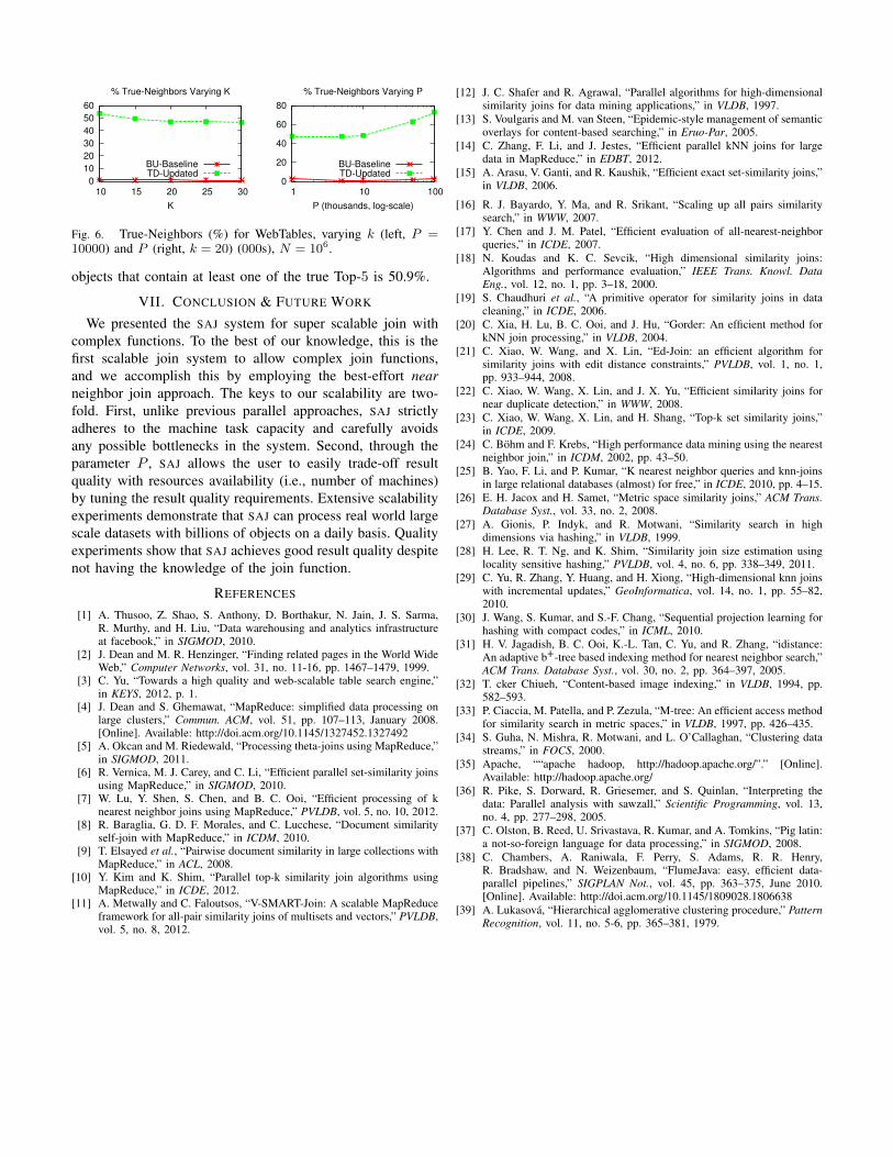
Precision. Finally, we again emphasize that having nearestneighbors is not crucial in our target application of findingrelated tables on the Web. We may fail to locate any ofthe most relevant tables, but the users can still be happywith the tables we return because they are quite relevant andmuch better than random tables. However, for the sake ofcompleteness, we also measured the percentage of nearestneighbors produced by our system for the WebTables dataset,as shown in Figure 6. We observe that we find a goodpercentage of nearest neighbors even though this is not the goalof SAJ. The number of nearest neighbors grows as P increases,approaching gracefully the exact solution. The impact of theTD phase is again significant.

We also measured the percentage of nearest neighbors forthe DBLP dataset using the default settings. The percentageof objects that contain at least one of the true Top-2 in theirneighbor list produced by SAJ is 17.8% and the percentage of

0

10

20

30

40

50

60

10 15 20 25 30

K

% True-Neighbors Varying K

BU-BaselineTD-Updated

0

20

40

60

80

1 10 100

P (thousands, log-scale)

% True-Neighbors Varying P

BU-BaselineTD-Updated

Fig. 6. True-Neighbors (%) for WebTables, varying k (left, P =10000) and P (right, k = 20) (000s), N = 106.

objects that contain at least one of the true Top-5 is 50.9%.

VII. CONCLUSION & FUTURE WORK

We presented the SAJ system for super scalable join withcomplex functions. To the best of our knowledge, this is thefirst scalable join system to allow complex join functions,and we accomplish this by employing the best-effort nearneighbor join approach. The keys to our scalability are two-fold. First, unlike previous parallel approaches, SAJ strictlyadheres to the machine task capacity and carefully avoidsany possible bottlenecks in the system. Second, through theparameter P , SAJ allows the user to easily trade-off resultquality with resources availability (i.e., number of machines)by tuning the result quality requirements. Extensive scalabilityexperiments demonstrate that SAJ can process real world largescale datasets with billions of objects on a daily basis. Qualityexperiments show that SAJ achieves good result quality despitenot having the knowledge of the join function.

REFERENCES

[1] A. Thusoo, Z. Shao, S. Anthony, D. Borthakur, N. Jain, J. S. Sarma,R. Murthy, and H. Liu, “Data warehousing and analytics infrastructureat facebook,” in SIGMOD, 2010.

[2] J. Dean and M. R. Henzinger, “Finding related pages in the World WideWeb,” Computer Networks, vol. 31, no. 11-16, pp. 1467–1479, 1999.

[3] C. Yu, “Towards a high quality and web-scalable table search engine,”in KEYS, 2012, p. 1.

[4] J. Dean and S. Ghemawat, “MapReduce: simplified data processing onlarge clusters,” Commun. ACM, vol. 51, pp. 107–113, January 2008.[Online]. Available: http://doi.acm.org/10.1145/1327452.1327492

[5] A. Okcan and M. Riedewald, “Processing theta-joins using MapReduce,”in SIGMOD, 2011.

[6] R. Vernica, M. J. Carey, and C. Li, “Efficient parallel set-similarity joinsusing MapReduce,” in SIGMOD, 2010.

[7] W. Lu, Y. Shen, S. Chen, and B. C. Ooi, “Efficient processing of knearest neighbor joins using MapReduce,” PVLDB, vol. 5, no. 10, 2012.

[8] R. Baraglia, G. D. F. Morales, and C. Lucchese, “Document similarityself-join with MapReduce,” in ICDM, 2010.

[9] T. Elsayed et al., “Pairwise document similarity in large collections withMapReduce,” in ACL, 2008.

[10] Y. Kim and K. Shim, “Parallel top-k similarity join algorithms usingMapReduce,” in ICDE, 2012.

[11] A. Metwally and C. Faloutsos, “V-SMART-Join: A scalable MapReduceframework for all-pair similarity joins of multisets and vectors,” PVLDB,vol. 5, no. 8, 2012.

[12] J. C. Shafer and R. Agrawal, “Parallel algorithms for high-dimensionalsimilarity joins for data mining applications,” in VLDB, 1997.

[13] S. Voulgaris and M. van Steen, “Epidemic-style management of semanticoverlays for content-based searching,” in Eruo-Par, 2005.

[14] C. Zhang, F. Li, and J. Jestes, “Efficient parallel kNN joins for largedata in MapReduce,” in EDBT, 2012.

[15] A. Arasu, V. Ganti, and R. Kaushik, “Efficient exact set-similarity joins,”in VLDB, 2006.

[16] R. J. Bayardo, Y. Ma, and R. Srikant, “Scaling up all pairs similaritysearch,” in WWW, 2007.

[17] Y. Chen and J. M. Patel, “Efficient evaluation of all-nearest-neighborqueries,” in ICDE, 2007.

[18] N. Koudas and K. C. Sevcik, “High dimensional similarity joins:Algorithms and performance evaluation,” IEEE Trans. Knowl. DataEng., vol. 12, no. 1, pp. 3–18, 2000.

[19] S. Chaudhuri et al., “A primitive operator for similarity joins in datacleaning,” in ICDE, 2006.

[20] C. Xia, H. Lu, B. C. Ooi, and J. Hu, “Gorder: An efficient method forkNN join processing,” in VLDB, 2004.

[21] C. Xiao, W. Wang, and X. Lin, “Ed-Join: an efficient algorithm forsimilarity joins with edit distance constraints,” PVLDB, vol. 1, no. 1,pp. 933–944, 2008.

[22] C. Xiao, W. Wang, X. Lin, and J. X. Yu, “Efficient similarity joins fornear duplicate detection,” in WWW, 2008.

[23] C. Xiao, W. Wang, X. Lin, and H. Shang, “Top-k set similarity joins,”in ICDE, 2009.

[24] C. Bohm and F. Krebs, “High performance data mining using the nearestneighbor join,” in ICDM, 2002, pp. 43–50.

[25] B. Yao, F. Li, and P. Kumar, “K nearest neighbor queries and knn-joinsin large relational databases (almost) for free,” in ICDE, 2010, pp. 4–15.

[26] E. H. Jacox and H. Samet, “Metric space similarity joins,” ACM Trans.Database Syst., vol. 33, no. 2, 2008.

[27] A. Gionis, P. Indyk, and R. Motwani, “Similarity search in highdimensions via hashing,” in VLDB, 1999.

[28] H. Lee, R. T. Ng, and K. Shim, “Similarity join size estimation usinglocality sensitive hashing,” PVLDB, vol. 4, no. 6, pp. 338–349, 2011.

[29] C. Yu, R. Zhang, Y. Huang, and H. Xiong, “High-dimensional knn joinswith incremental updates,” GeoInformatica, vol. 14, no. 1, pp. 55–82,2010.

[30] J. Wang, S. Kumar, and S.-F. Chang, “Sequential projection learning forhashing with compact codes,” in ICML, 2010.

[31] H. V. Jagadish, B. C. Ooi, K.-L. Tan, C. Yu, and R. Zhang, “idistance:An adaptive b+-tree based indexing method for nearest neighbor search,”ACM Trans. Database Syst., vol. 30, no. 2, pp. 364–397, 2005.

[32] T. cker Chiueh, “Content-based image indexing,” in VLDB, 1994, pp.582–593.

[33] P. Ciaccia, M. Patella, and P. Zezula, “M-tree: An efficient access methodfor similarity search in metric spaces,” in VLDB, 1997, pp. 426–435.

[34] S. Guha, N. Mishra, R. Motwani, and L. O’Callaghan, “Clustering datastreams,” in FOCS, 2000.

[35] Apache, ““apache hadoop, http://hadoop.apache.org/”.” [Online].Available: http://hadoop.apache.org/

[36] R. Pike, S. Dorward, R. Griesemer, and S. Quinlan, “Interpreting thedata: Parallel analysis with sawzall,” Scientific Programming, vol. 13,no. 4, pp. 277–298, 2005.

[37] C. Olston, B. Reed, U. Srivastava, R. Kumar, and A. Tomkins, “Pig latin:a not-so-foreign language for data processing,” in SIGMOD, 2008.

[38] C. Chambers, A. Raniwala, F. Perry, S. Adams, R. R. Henry,R. Bradshaw, and N. Weizenbaum, “FlumeJava: easy, efficient data-parallel pipelines,” SIGPLAN Not., vol. 45, pp. 363–375, June 2010.[Online]. Available: http://doi.acm.org/10.1145/1809028.1806638

[39] A. Lukasova, “Hierarchical agglomerative clustering procedure,” PatternRecognition, vol. 11, no. 5-6, pp. 365–381, 1979.