NOTES SUBJECT: DATA STRUCTURES USING C

SUBJECT CODE: NCS-301 BRANCH: CSE

SEM: 3rd SESSION: 2014-15

Evaluation Scheme Subject

Code Name of Subject

Periods Evaluation Scheme Subject Total

Credit L T P CT TA TOTAL ESE

NCS-301 Data Structures

Using C

3 1 0 30 20 50 100 150 4

Asst. Prof. Swimpy Pahuja & Priyanka Gupta

CSE Department, AKGEC Ghaziabad

CONTENTS

UNIT-1 INTRODUCTION

1.1 BASIC TERMINOLOGY: ELEMENTARY DATA ORGANIZATION 1.1.1 Data and Data Item

1.1.2 Data Type 1.1.3 Variable 1.1.4 Record

1.1.5 Program 1.1.6 Entity 1.1.7 Entity Set 1.1.8 Field 1.1.9 File 1.1.10 Key 1.2 ALGORITHM 1.3 EFFICIENCY OF AN ALGORITHM 1.4 TIME AND SPACE COMPLEXITY 1.5 ASYMPTOTIC NOTATIONS 1.5.1 Asymptotic 1.5.2 Asymptotic Notations

1.5.2.1 Big-Oh Notation (O) 1.5.2.2 Big-Omega Notation (Ω) 1.5.2.3 Big-Theta Notation (Θ)

1.5.3 Time Space Trade-off 1.6 ABSTRACT DATA TYPE 1.7 DATA STRUCTURE

1.7.1 Need of data structure 1.7.2 Selecting a data structure 1.7.3 Type of data structure 1.7.3.1 Static data structure 1.7.3.2 Dynamic data structure 1.7.3.3 Linear Data Structure 1.7.3.4 Non-linear Data Structure 1.8 A BRIEF DESCRIPTION OF DATA STRUCTURES

1.8.1 Array 1.8.2 Linked List 1.8.3 Tree 1.8.4 Graph 1.8.5 Queue 1.8.6 Stack 1.9 DATA STRUCTURES OPERATIONS 1.10 ARRAYS: DEFINITION 1.10.1 Representation of One-Dimensional Array

1.10.2 Two-Dimensional Arrays 1.10.3 Representation of Three& Four Dimensional Array 1.10.4 Operations on array

1.10.5 Applications of array 1.10.6 Sparse matrix 1.11 STATIC AND DYNAMIC MEMORY ALLOCATION 1.12 LINKED LIST 1.12.1 Representation of Linked list in memory

1.12.2 Types of linked lists 1.12.3 The Operations on the Linear Lists 1.12.4 Comparison of Linked List and Array

1.12.5 Advantages 1.12.6 Operations on Linked List

1.12.7 Doubly Linked Lists 1.12.8 Circular Linked List 1.12.9 Polynomial representation and addition

1.13 GENERALIZED LINKED LIST

UNIT-2 STACKS 2.1 STACKS 2.2 PRIMITIVE STACK OPERATIONS 2.3 ARRAY AND LINKED IMPLEMENTATION OF STACK IN C 2.4 APPLICATION OF THE STACK (ARITHMETIC EXPRESSIONS) 2.5 EVALUATION OF POSTFIX EXPRESSION 2.6 RECURSION

2.6.1 Simulation of Recursion 2.6.1.1 Tower of Hanoi Problem

2.6.2 Tail recursion 2.7 QUEUES 2.8 DEQUEUE (OR) DEQUE (DOUBLE ENDED QUEUE) 2.9 PRIORITY QUEUE UNIT-3 TREES 3.1 TREES TERMINOLOGY 3.2 BINARY TREE 3.3 TRAVERSALS 3.4 BINARY SEARCH TREES 3.4.1 Non-Recursive Traversals 3.4.2 Array Representation of Complete Binary Trees 3.4.3 Heaps 3.5 DYNAMIC REPRESENTATION OF BINARY TREE 3.6 COMPLETE BINARY TREE 3.6.1 Algebraic Expressions 3.6.2 Extended Binary Tree: 2-Trees 3.7 TREE TRAVERSAL ALGORITHMS

3.8 THREADED BINARY TREE 3.9 HUFFMAN CODE UNIT-4 GRAPHS 4.1 INTRODUCTION 4.2 TERMINOLOGY 4.3 GRAPH REPRESENTATIONS

4.3.1 Sequential representation of graphs 4.3.2 Linked List representation of graphs

4.4 GRAPH TRAVERSAL 4.5 CONNECTED COMPONENT 4.6 SPANNING TREE

4.6.1 Kruskal’s Algorithm 4.6.2Prim’s Algorithm

4.7 TRANSITIVE CLOSURE AND SHORTEST PATH ALGORITHM 4.6.1 Dijikstra’s Algorithm 4.6.2Warshall’s Algorithm

4.8 INTRODUCTION TO ACTIVITY NETWORKS UNIT-5 SEARCHING 5.1 SEARCHING 5.1.1 Linear Search or Sequential Search 5.1.2 Binary Search 5.2 INTRODUCTION TO SORTING 5.3 TYPES OF SORTING 5.3.1 Insertion sort 5.3.2 Selection Sort 5.3.3 Bubble Sort 5.3.4 Quick Sort 5.3.5 Merge Sort 5.3.6 Heap Sort 5.3.7 Radix Sort 5.4 PRACTICAL CONSIDERATION FOR INTERNAL SORTING 5.5 SEARCH TREES 5.5.1 Binary Search Trees 5.5.2 AVL Trees 5.5.3 M-WAY Search Trees 5.5.4 B Trees 5.5.5 B+ Trees 5.6 HASHING 5.6.1 Hash Function 5.6.2 Collision Resolution Techniques 5.7 STORAGE MANGMENT 5.7.1 Garbage Collection 5.7.2Compaction

AJAY KUMAR GARG ENGINEERING COLLEGE GHAZIABAD

DEPARTMENT OF COMPUTER SCIENCE AND ENGINEERING

COURSE: B.Tech. SEMESTER: III

SUBJECT CODE: NCS-301 L: 3 T: 1 P: 0

NCS-301: DATA STRUCTURES USING C

Prerequisite: Students should be familiar with procedural language like C and concepts of mathematics Objective: To make students understand specification, representation, and implementation of data types and data structures, basic techniques of algorithm analysis, recursive methods, applications of Data Structures. Unit - I Introduction: Basic Terminology, Elementary Data Organization, Algorithm, Efficiency of an Algorithm, Time and Space Complexity, Asymptotic notations: Big-Oh, Time-Space trade-off. Abstract Data Types (ADT) Arrays: Definition, Single and Multidimensional Arrays, Representation of Arrays: Row Major Order, and Column Major Order, Application of arrays, Sparse Matrices and their representations. Linked lists: Array Implementation and Dynamic Implementation of Singly Linked Lists, Doubly Linked List, Circularly Linked List, Operations on a Linked List. Insertion, Deletion, Traversal, Polynomial Representation and Addition, Generalized Linked List. Unit – II Stacks: Abstract Data Type, Primitive Stack operations: Push & Pop, Array and Linked Implementation of Stack in C, Application of stack: Prefix and Postfix Expressions, Evaluation of postfix expression, Recursion, Tower of Hanoi Problem, Simulating Recursion, Principles of recursion, Tail recursion, Removal of recursion Queues, Operations on Queue: Create, Add, Delete, Full and Empty, Circular queues, Array and linked implementation of queues in C, Dequeue and Priority Queue. Unit – III Trees: Basic terminology, Binary Trees, Binary Tree Representation: Array Representation and Dynamic Representation, Complete Binary Tree, Algebraic Expressions, Extended Binary Trees, Array and Linked Representation of Binary trees, Tree Traversal algorithms: Inorder, Preorder and Postorder, Threaded Binary trees, Traversing Threaded Binary trees, Huffman algorithm.

Unit – IV Unit- IV Graphs: Terminology, Sequential and linked Representations of Graphs: Adjacency Matrices, Adjacency List, Adjacency Multi list, Graph Traversal : Depth First Search and Breadth First Search, Connected Component, Spanning Trees, Minimum Cost Spanning Trees: Prims and Kruskal algorithm. Transistive Closure and Shortest Path algorithm: Warshal Algorithm and Dijikstra Algorithm, Introduction to Activity Networks. Unit – V Searching : Sequential search, Binary Search, Comparison and Analysis Internal Sorting: Insertion Sort, Selection, Bubble Sort, Quick Sort, Two Way Merge Sort, Heap Sort, Radix Sort, Practical consideration for Internal Sorting. Search Trees: Binary Search Trees(BST), Insertion and Deletion in BST, Complexity of Search Algorithm, AVL trees, Introduction to m-way Search Trees, B Trees & B+ Trees . Hashing: Hash Function, Collision Resolution Strategies Storage Management: Garbage Collection and Compaction. References: 1. Aaron M. Tenenbaum,YedidyahLangsam and Moshe J. Augenstein “Data Structures Using C

and C++”, PHI Learning Private Limited, Delhi India. 2. Horowitz and Sahani, “Fundamentals of Data Structures”, Galgotia Publications Pvt Ltd

Delhi India. 3. A.K. Sharma ,Data Structure Using C, Pearson Education India. 4. Rajesh K. Shukla, “Data Structure Using C and C++” Wiley Dreamtech Publication. 5. Lipschutz, “Data Structures” Schaum’s Outline Series, Tata Mcgraw-hill Education (India)

Pvt. Ltd . 6. Michael T. Goodrich, Roberto Tamassia, David M. Mount “Data Structures and Algorithms in

C++”, Wiley India. 7. P.S. Deshpandey, “C and Datastructure”, Wiley Dreamtech Publication. 8. R. Kruse etal, “Data Structures and Program Design in C”, Pearson Education 9. Berztiss, A.T.: Data structures, Theory and Practice :, Academic Press. 10. Jean Paul Trembley and Paul G. Sorenson, “An Introduction to Data Structures with

applications”, McGraw Hill.

UNIT-1

1.1 BASIC TERMINOLOGY: ELEMENTARY DATA ORGANIZATION 1.1.1 Data and Data Item Data are simply collection of facts and figures. Data are values or set of values. A data item refers to a single unit of values. Data items that are divided into sub items are group items; those that are not are called elementary items. For example, a student’s name may be divided into three sub items – [first name, middle name and last name] but the ID of a student would normally be treated as a single item.

In the above example ( ID, Age, Gender, First, Middle, Last, Street, Area ) are elementary data items, whereas (Name, Address ) are group data items. 1.1.2 Data Type Data type is a classification identifying one of various types of data, such as floating-point, integer, or Boolean, that determines the possible values for that type; the operations that can be done on values of that type; and the way values of that type can be stored. It is of two types: Primitive and non-primitive data type. Primitive data type is the basic data type that is provided by the programming language with built-in support. This data type is native to the language and is supported by machine directly while non-primitive data type is derived from primitive data type. For example- array, structure etc. 1.1.3 Variable It is a symbolic name given to some known or unknown quantity or information, for the purpose of allowing the name to be used independently of the information it represents. A variable name in computer source code is usually associated with a data storage location and thus also its contents and these may change during the course of program execution. 1.1.4 Record Collection of related data items is known as record. The elements of records are usually called fields or members. Records are distinguished from arrays by the fact that their number of fields is typically fixed, each field has a name, and that each field may have a different type.

1.1.5 Program A sequence of instructions that a computer can interpret and execute is termed as program. 1.1.6 Entity An entity is something that has certain attributes or properties which may be assigned some values. The values themselves may be either numeric or non-numeric. Example:

1.1.7 Entity Set An entity set is a group of or set of similar entities. For example, employees of an organization, students of a class etc. Each attribute of an entity set has a range of values, the set of all possible values that could be assigned to the particular attribute. The term “information” is sometimes used for data with given attributes, of, in other words meaningful or processed data. 1.1.8 Field A field is a single elementary unit of information representing an attribute of an entity, a record is the collection of field values of a given entity and a file is the collection of records of the entities in a given entity set. 1.1.9 File File is a collection of records of the entities in a given entity set. For example, file containing records of students of a particular class. 1.1.10 Key A key is one or more field(s) in a record that take(s) unique values and can be used to distinguish one record from the others. 1.2 ALGORITHM A well-defined computational procedure that takes some value, or a set of values, as input and produces some value, or a set of values, as output. It can also be defined as sequence of computational steps that transform the input into the output. An algorithm can be expressed in three ways:- (i) in any natural language such as English, called pseudo code. (ii) in a programming language or (iii) in the form of a flowchart.

1.3 EFFICIENCY OF AN ALGORITHM In computer science, algorithmic efficiency are the properties of an algorithm which relate to the amount of resources used by the algorithm. An algorithm must be analyzed to determine its

resource usage. Algorithmic efficiency can be thought of as analogous to engineering productivity for a repeating or continuous process.

For maximum efficiency we wish to minimize resource usage. However, the various resources (e.g. time, space) can not be compared directly, so which of two algorithms is considered to be more efficient often depends on which measure of efficiency is being considered as the most important, e.g. is the requirement for high speed, or for minimum memory usage, or for some other measure. It can be of various types:

• Worst case efficiency: It is the maximum number of steps that an algorithm can take for any collection of data values.

• Best case efficiency: It is the minimum number of steps that an algorithm can take any collection of data values.

• Average case efficiency: It can be defined as - the efficiency averaged on all possible inputs - must assume a distribution of the input - We normally assume uniform distribution (all keys are equally probable) If the input has size n, efficiency will be a function of n 1.4 TIME AND SPACE COMPLEXITY Complexity of algorithm is a function of size of input of a given problem instance which determines how much running time/memory space is needed by the algorithm in order to run to completion. Time Complexity: Time complexity of an algorithm is the amount of time it needs in order to run to completion. Space Complexity: Space Complexity of an algorithm is the amount of space it needs in order to run to completion. There are two points which we should consider about computer programming:- (i) An appropriate data structure and (ii) An appropriate algorithm. 1.5 ASYMPTOTIC NOTATIONS

1.5.1 Asymptotic It means a line that continually approaches a given curve but does not meet it at any finite distance.

Example

x is asymptotic with x + 1 as shown in graph.

Asymptotic may also be defined as a way to describe the behavior of functions in the limit or without bounds.

Let f(x) and g(x) be functions from the set of real

numbers to the set of real numbers.

We say that f and g are asymptotic and write f(x) ≈ g(x) if

f(x) / g(x) = c (constant)

1.5.2 Asymptotic Notations

1.7.2.1 Big-Oh Notation (O)

It provides possibly asymptotically tight upper bound for f(n) and it does not give best case complexity but can give worst case complexity.

Let f be a nonnegative function. Then we define the three most common asymptotic bounds as follows.

We say that f(n) is Big-O of g(n), written as f(n) = O(g(n)), iff there are positive constants c and n0 such that

0 ≤ f(n) ≤ c g(n) for all n ≥ n0

If f(n) = O(g(n)), we say that g(n) is an upper bound on f(n).

Example - n2 + 50n = O(n2)

0 ≤ h(n) ≤ cg(n)

0 ≤ n2 + 50n ≤ cn2

0/n2 ≤ n2/n2 + 50n/n2 ≤ cn2/n2 Divide by n2

0 ≤ 1 + 50/n ≤ c Note that 50/n → 0 as n → ∞

Pick n = 50

0 ≤ 1 + 50/50 = 2 ≤ c = 2 With c=2

0 ≤ 1 + 50/n0 ≤ 2 Find n0

-1 ≤ 50/n0 ≤ 1

-20n0 ≤ 50 ≤ n0 = 50 n0=50

0 ≤ n2 + 50n ≤ 2n2 ∀ n ≥ n0=50, c=2

1.7.2.2 Big-Omega Notation (Ω)

It provides possibly asymptotically tight lower bound for f(n) and it does not give worst case

complexity but can give best case complexity

f(n) is said to be Big-Omega of g(n), written as f(n) = Ω(g(n)), iff there are positive constants c and n0 such that

0 ≤ c g(n) ≤ f(n) for all n ≥ n0

If f(n) = Ω(g(n)), we say that g(n) is a lower bound on f(n).

Example - n3 = Ω(n2) with c=1 and n0=1

0 ≤ cg(n) ≤ h(n) 0 ≤ 1*12 = 1 ≤ 1 = 13

0 ≤ cg(n) ≤ h(n)

0 ≤ cn2 ≤ n3

0/n2 ≤ cn2/n2 ≤ n3/n2

0 ≤ c ≤ n

0 ≤ 1 ≤ 1 with c=1 and n0=1 since n increases.

n = ∞

1.7.2.3 Big-Theta Notation (Θ)

• We say that f(n) is Big-Theta of g(n), written as f(n) = Θ(g(n)), iff there are positive constants c1, c2 and n0 such that

0 ≤ c1 g(n) ≤ f(n) ≤ c2 g(n) for all n ≥ n0

Equivalently, f(n) = Θ(g(n)) if and only if f(n) = O(g(n)) and f(n) = Ω(g(n)). If f(n) = Θ(g(n)), we

say that g(n) is a tight bound on f(n).

Example - n2/2-2n = Θ(n2)

c1g(n) ≤ h(n) ≤ c2g(n)

c1n2 ≤ n2/2-2n ≤ c2n2

c1n2/n2 ≤ n2/2n2-2n/n2 ≤ c2n2/n2 Divide by n2

c1 ≤ 1/2-2/n ≤ c2

O Determine c2 = ½

½-2/n ≤ c2 = ½ ½-2/n = ½

maximum of ½-2/n

Ω Determine c1 = 1/10

0 < c1 ≤ ½-2/n 0 < c1 minimum when n=5

0 < c1 ≤ ½-2/5

0 < c1 ≤ 5/10-4/10 = 1/10

n0 Determine n0 = 5

c1 ≤ ½-2/n0 ≤ c2

1/10 ≤ ½-2/n0 ≤ ½

1/10-½ ≤ -2/n0 ≤ 0 Subtract ½

-4/10 ≤ -2/n0 ≤ 0

-4/10 n0 ≤ -2 ≤ 0 Multiply by n0

-n0 ≤ -2*10/4 ≤ 0 Multiply by 10/4

n0 ≥ 2*10/4 ≥ 0 Multiply by -1

n0 ≥ 5 ≥ 0

n0 ≥ 5 n0 = 5 satisfies

Θ 0 < c1n2 ≤ n2/2-2n ≤ c2n2 ∀n ≥ n0 with c1=1/10, c2=½ and n0=5

1.5.3 Time Space Trade-off The best algorithm to solve a given problem is one that requires less memory space and less time to run to completion. But in practice, it is not always possible to obtain both of these objectives. One algorithm may require less memory space but may take more time to complete its execution. On the other hand, the other algorithm may require more memory space but may take less time to run to completion. Thus, we have to sacrifice one at the cost of other. In other words, there is Space-Time trade-off between algorithms.

If we need an algorithm that requires less memory space, then we choose the first algorithm at the cost of more execution time. On the other hand if we need an algorithm that requires less time for execution, then we choose the second algorithm at the cost of more memory space. 1.6 ABSTRACT DATA TYPE

It can be defined as a collection of data items together with the operations on the data. The word “abstract” refers to the fact that the data and the basic operations defined on it are being studied independently of how they are implemented. It involves what can be done with the data, not how has to be done. For ex, in the below figure the user would be involved in checking that what can be done with the data collected not how it has to be done.

An implementation of ADT consists of storage structures to store the data items and algorithms for basic operation. All the data structures i.e. array, linked list, stack, queue etc are examples of ADT.

1.7 DATA STRUCTURE In computer science, a data structure is a particular way of storing and organizing data in a computer’s memory so that it can be used efficiently. Data may be organized in many different ways; the logical or mathematical model of a particular organization of data is called a data structure. The choice of a particular data model depends on the two considerations first; it must be rich enough in structure to mirror the actual relationships of the data in the real world. On the other hand, the structure should be simple enough that one can effectively process the data whenever necessary. 1.7.1 Need of data structure

• It gives different level of organization data. • It tells how data can be stored and accessed in its elementary level. • Provide operation on group of data, such as adding an item, looking up highest priority

item. • Provide a means to manage huge amount of data efficiently.

• Provide fast searching and sorting of data.

1.7.2 Selecting a data structure Selection of suitable data structure involve following steps –

• Analyze the problem to determine the resource constraints a solution must meet. • Determine basic operation that must be supported. Quantify resource constraint for each

operation • Select the data structure that best meets these requirements. • Each data structure has cost and benefits. Rarely is one data structure better than other in

all situations. A data structure require : Ø Space for each item it stores Ø Time to perform each basic operation Ø Programming effort.

Each problem has constraints on available time and space. Best data structure for the task requires careful analysis of problem characteristics. 1.7.3 Type of data structure 1.7.3.1 Static data structure A data structure whose organizational characteristics are invariant throughout its lifetime. Such structures are well supported by high-level languages and familiar examples are arrays and records. The prime features of static structures are (a) None of the structural information need be stored explicitly within the elements – it is often held in a distinct logical/physical header; (b) The elements of an allocated structure are physically contiguous, held in a single segment of memory; (c) All descriptive information, other than the physical location of the allocated structure, is determined by the structure definition; (d) Relationships between elements do not change during the lifetime of the structure. 1.7.3.2 Dynamic data structure A data structure whose organizational characteristics may change during its lifetime. The adaptability afforded by such structures, e.g. linked lists, is often at the expense of decreased efficiency in accessing elements of the structure. Two main features distinguish dynamic structures from static data structures. Firstly, it is no longer possible to infer all structural information from a header; each data element will have to contain information relating it logically to other elements of the structure. Secondly, using a single block of contiguous storage is often not appropriate, and hence it is necessary to provide some storage management scheme at run-time. 1.7.3.3 Linear Data Structure A data structure is said to be linear if its elements form any sequence. There are basically two ways of representing such linear structure in memory. a) One way is to have the linear relationships between the elements represented by means of sequential memory location. These linear structures are called arrays.

b) The other way is to have the linear relationship between the elements represented by means of pointers or links. These linear structures are called linked lists. The common examples of linear data structure are arrays, queues, stacks and linked lists. 1.7.3.4 Non-linear Data Structure This structure is mainly used to represent data containing a hierarchical relationship between elements. E.g. graphs, family trees and table of contents. 1.9 A BRIEF DESCRIPTION OF DATA STRUCTURES 1.8.1 Array The simplest type of data structure is a linear (or one dimensional) array. A list of a finite number n of similar data referenced respectively by a set of n consecutive numbers, usually 1, 2, 3 . . . . . . . n. if we choose the name A for the array, then the elements of A are denoted by subscript notation

A 1, A 2, A 3 . . . . A n or by the parenthesis notation

A (1), A (2), A (3) . . . . . . A (n) or by the bracket notation

A [1], A [2], A [3] . . . . . . A [n] Example: A linear array A[8] consisting of numbers is pictured in following figure.

1.8.2 Linked List A linked list or one way list is a linear collection of data elements, called nodes, where the linear order is given by means of pointers. Each node is divided into two parts:

• The first part contains the information of the element/node • The second part contains the address of the next node (link /next pointer field) in the list.

There is a special pointer Start/List contains the address of first node in the list. If this special pointer contains null, means that List is empty. Example:

1.8.3 Tree Data frequently contain a hierarchical relationship between various elements. The data structure which reflects this relationship is called a rooted tree graph or, simply, a tree.

1.8.4 Graph Data sometimes contains a relationship between pairs of elements which is not necessarily hierarchical in nature, e.g. an airline flights only between the cities connected by lines. This data structure is called Graph. 1.8.5 Queue A queue, also called FIFO system, is a linear list in which deletions can take place only at one end of the list, the Font of the list and insertion can take place only at the other end Rear. 1.8.6 Stack It is an ordered group of homogeneous items of elements. Elements are added to and removed from the top of the stack (the most recently added items are at the top of the stack). The last element to be added is the first to be removed (LIFO: Last In, First Out). 1.9 DATA STRUCTURES OPERATIONS The data appearing in our data structures are processed by means of certain operations. In fact, the particular data structure that one chooses for a given situation depends largely in the frequency with which specific operations are performed. The following four operations play a major role in this text:

• Traversing: accessing each record/node exactly once so that certain items in the record may be processed. (This accessing and processing is sometimes called “visiting” the record.)

• Searching: Finding the location of the desired node with a given key value, or finding the locations of all such nodes which satisfy one or more conditions.

• Inserting: Adding a new node/record to the structure. • Deleting: Removing a node/record from the structure.

1.10 ARRAYS: DEFINITION

C programming language provides a data structure called the array, which can store a fixed-size sequential collection of elements of the same type. An array is used to store a collection of data, but it is often more useful to think of an array as a collection of variables of the same type.

Instead of declaring individual variables, such as number0, number1, ..., and number99, you declare one array variable such as numbers and use numbers[0], numbers[1], and ..., numbers[99] to represent individual variables. A specific element in an array is accessed by an index.

All arrays consist of contiguous memory locations. The lowest address corresponds to the first element and the highest address to the last element.

The array may be categorized into –

• One dimensional array

• Two dimensional array

• Multidimensional array

1.10.1 Representation of One-Dimensional Array

In Pascal language we can define array as

VAR X: array [ 1 … N] of integer or any other type

That’s means the structure contains a set of data elements, numbered (N), for example called (X), its defined as type of element, the second type is the index type, is the type of values used to access individual element of the array, the value of index is

1<= I =< N

By this definition the compiler limits the storage region to storing set of element, and the first location is individual element of array , and this called the Base Address, let’s be as 500. Base Address (501) and like for the all elements and used the index I, by its value are range 1<= I => N according to Base Index (500), by using this relation:

Location ( X[I] ) = Base Address + (I-1)

When the requirement to bounding the forth element (I=4):

Location ( X[4] ) = 500 + (4-1)

= 500 +3

= 503

So the address of forth element is 503 because the first element in 500.

When the program indicate or dealing with element of array in any instruction like (write (X [I]), read (X [I] ) ), the compiler depend on going relation to bounding the requirement address.

1.10.2 Two-Dimensional Arrays

The simplest form of the multidimensional array is the two-dimensional array. A two-dimensional array is, in essence, a list of one-dimensional arrays. To declare a two-dimensional integer array of size x,y you would write something as follows:

type arrayName [ x ][ y ];

Where type can be any valid C data type and arrayName will be a valid C identifier. A two-dimensional array can be think as a table which will have x number of rows and y number of columns. A 2-dimensional array a, which contains three rows and four columns can be shown as below:

Thus, every element in array a is identified by an element name of the form a[ i ][ j ], where a is the name of the array, and i and j are the subscripts that uniquely identify each element in a. 1.10.2.1 Representation of two dimensional arrays in memory A two dimensional ‘m x n’ Array A is the collection of m X n elements. Programming language stores the two dimensional array in one dimensional memory in either of two ways-

• Row Major Order: First row of the array occupies the first set of memory locations reserved for the array; Second row occupies the next set, and so forth.

To determine element address A[i,j]:

Location ( A[ i,j ] ) =Base Address + ( N x ( I - 1 ) ) + ( j - 1 )

For example:

Given an array [1…5,1…7] of integers. Calculate address of element T[4,6], where BA=900.

Sol) I = 4 , J = 6

M= 5 , N= 7

Location (T [4,6]) = BA + (7 x (4-1)) + (6-1)

= 900+ (7 x 3) +5

= 900+ 21+5

= 926

• Column Major Order: Order elements of first column stored linearly and then comes

elements of next column.

To determine element address A[i,j]:

Location ( A[ i,j ] ) =Base Address + ( M x ( j - 1 ) ) + ( i - 1 )

For example:

Given an array [1…6,1…8] of integers. Calculate address element T[5,7], where BA=300

Sol) I = 5 , J = 7

M= 6 , N= 8

Location (T [4,6]) = BA + (6 x (7-1)) + (5-1)

= 300+ (6 x 6) +4

= 300+ 36+4

= 340

1.10.3 Representation of Three& Four Dimensional Array

By the same way we can determine address of element for three and four dimensional array:

Three Dimensional Array

To calculate address of element X[ i,j,k] using row-major order :

Location ( X[i,j,k] )=BA + MN (k-1) + N (i-1) + (j-1)

using column-major order

Location ( X[i,j,k] )=BA + MN (k-1) + M (j-1) + (i-1)

Four Dimensional Array

To calculate address of element X[ i,j,k] using row-major order :

Location ( Y[i,j,k,l] )=BA + MNR (l-1) +MN (k-1) +N (i-1) + (j-1)

using column-major order

Location ( Y[i,j,k,l] )=BA + MNR (l-1) +MN (k-1) +M (j-1) + (i-1)

For example:

Given an array [ 1..8, 1..5, 1..7 ] of integers. Calculate address of element A[5,3,6], by using rows &columns methods, if BA=900?

Sol) The dimensions of A are :

M=8 , N=5, R=7

i=5, j=3, k=6

Rows- wise

Location (A[i,j,k]) = BA + MN(k-1) + N(i-1) + (j-1)

Location (A[5,3,6]) = 900 + 8x5(6-1) + 5(5-1) + (3-1)

= 900 + 40 x 5 +5 x 4 + 2

= 900 + 200 +20 +2

= 1122

Columns- wise

Location (A[i,j,k]) = BA + MN(k-1) + M(j-1) + (i-1)

Location (A[5,3,6]) = 900 + 8x5(6-1) + 8(3-1) + (5-1)

= 900 + 40 x 5 +8 x 2 + 4

= 900 + 200 +16 +4

1.10.4 Operations on array a) Traversing: means to visit all the elements of the array in an operation is called traversing. b) Insertion: means to put values into an array c) Deletion / Remove: to delete a value from an array. d) Sorting: Re-arrangement of values in an array in a specific order (Ascending or Descending) is called sorting. e) Searching: The process of finding the location of a particular element in an array is called searching. a) Traversing in Linear Array: It means processing or visiting each element in the array exactly once; Let ‘A’ is an array stored in the computer’s memory. If we want to display the contents of ‘A’, it has to be traversed i.e. by accessing and processing each element of ‘A’ exactly once.

The alternate algorithm for traversing (using for loop) is :

This program will traverse each element of the array to calculate the sum and then calculate & print the average of the following array of integers. ( 4, 3, 7, -1, 7, 2, 0, 4, 2, 13)

#include <iostream.h> #define size 10 // another way int const size = 10 int main() int x[10]=4,3,7,-1,7,2,0,4,2,13, i, sum=0,LB=0, UB=size; float av; for(i=LB,i<UB;i++) sum = sum + x[i]; av = (float)sum/size; cout<< “The average of the numbers= “<<av<<endl; return 0; b) Sorting in Linear Array: Sorting an array is the ordering the array elements in ascending (increasing from min to max) or descending (decreasing from max to min) order. Bubble Sort: The technique we use is called “Bubble Sort” because the bigger value gradually bubbles their way up to the top of array like air bubble rising in water, while the small values sink to the bottom of array. This technique is to make several passes through the array. On each pass, successive pairs of elements are compared. If a pair is in increasing order (or the values are identical), we leave the values as they are. If a pair is in decreasing order, their values are swapped in the array.

/* This program sorts the array elements in the ascending order using bubble sort method */ #include <iostream.h> int const SIZE = 6 void BubbleSort(int [ ], int); int main() int a[SIZE]= 77,42,35,12,101,6; int i; cout<< “The elements of the array before sorting\n”; for (i=0; i<= SIZE-1; i++) cout<< a[i]<<”, “; BubbleSort(a, SIZE); cout<< “\n\nThe elements of the array after sorting\n”; for (i=0; i<= SIZE-1; i++) cout<< a[i]<<”, “; return 0; void BubbleSort(int A[ ], int N) int i, pass, hold; for (pass=1; pass<= N-1; pass++) for (i=0; i<= SIZE-pass; i++) if(A[i] >A[i+1]) hold =A[i]; A[i]=A[i+1]; A[i+1]=hold;

1.10.5 Applications of array

Arrays are used to implement mathematical vectors and matrices, as well as other kinds of rectangular tables. Many databases, small and large, consist of (or include) one-dimensional arrays whose elements are records.

Arrays are used to implement other data structures, such as heaps, hash tables, deques, queues, stacks, strings, and VLists.

One or more large arrays are sometimes used to emulate in-program dynamic memory allocation, particularly memory pool allocation. Historically, this has sometimes been the only way to allocate "dynamic memory" portably.

Arrays can be used to determine partial or complete control flow in programs, as a compact alternative to (otherwise repetitive) multiple IF statements. They are known in this context as control tables and are used in conjunction with a purpose built interpreter whose control flow is altered according to values contained in the array.

1.10.6 Sparse matrix

Matrix with maximum zero entries is termed as sparse matrix. It can be represented as:

Ø Lower triangular matrix: It has non-zero entries on or below diagonal.

Ø Upper Triangular matrix: It has non-zero entries on or above diagonal.

Ø Tri-diagonal matrix: It has non-zero entries on diagonal and at the places immediately above or below diagonal.

1.11 STATIC AND DYNAMIC MEMORY ALLOCATION

In many programming environments memory allocation to variables can be of two types static memory allocation and dynamic memory allocation. Both differ on the basis of time when memory is allocated. In static memory allocation memory is allocated to variable at compile time whereas in dynamic memory allocation memory is allocated at the time of execution. Other

differences between both memory allocation techniques are summarized below-

1.12 LINKED LIST A linked list or one way list is a linear collection of data elements, called nodes, where the linear order is given by means of “pointers”. Each node is divided into two parts. Ø The first part contains the information of the element. Ø The second part called the link field contains the address of the next node in the list.

To see this more clearly lets look at an example:

The Head is a special pointer variable which contains the address of the first node of the list. If there is no node available in the list then Head contains NULLvalue that means, List is empty. The left part of the each node represents the information part of the node, which may contain an

entire record of data (e.g. ID, name, marks, age etc). the right part represents pointer/link to the next node. The next pointer of the last node is null pointer signal the end of the list. 1.12.1 Representation of Linked list in memory

Linked list is maintained in memory by two linear arrays: INFO and LINK such that INFO [K] and LINK [K] contain respectively the information part and the next pointer field of node of LIST. LIST also requires a variable name such as START which contains the location of the beginning of the list and the next pointer denoted by NULL which indicates the end of the LIST.

1.12.4 Types of linked lists

– Singly linked list • Begins with a pointer to the first node • Terminates with a null pointer • Only traversed in one direction

– Circular, singly linked • Pointer in the last node points back to the first node

– Doubly linked list • Two “start pointers” – first element and last element • Each node has a forward pointer and a backward pointer • Allows traversals both forwards and backwards

– Circular, doubly linked list • Forward pointer of the last node points to the first node and backward

pointer of the first node points to the last node – Header Linked List

• Linked list contains a header node that contains information regarding complete linked list.

1.12.3 The Operations on the Linear Lists Various operations are: 1- Search: This operation involves the searching of an element in the linked list. 2- Additional (Inserting) : To add new node to data structure. 3- Deletion : To delete a node from data structure. 4- Merge : To merge two structures or more to constituting one structure. 5- Split : To divide data structure to two structures or more. 6- Counting : counting some of items or nodes in data structure.

7- Copying : copy data of data structure to another data structure. 8- Sort : sort items or nodes in data structure according to the value of the field or set of fields. 9- Access : To access from node or item to another one may be need some of purposes to test or change...etc. 1.12.4 Comparison of Linked List and Array Comparison between array and linked list are summarized in following table –

1.12.5 Advantages List of data can be stored in arrays but linked structures (pointers) provide several advantages: A linked list is appropriate when the number of data elements to be represented in data structure is unpredictable. It also appropriate when there are frequently insertions & deletions occurred in the list. Linked lists are dynamic, so the length of a list can increase or decrease as necessary. 1.12.6 Operations on Linked List There are several operations associated with linked list i.e. a) Traversing a Linked List Suppose we want to traverse LIST in order to process each node exactly once. The traversing algorithm uses a pointer variable PTR which points to the node that is currently being processed. Accordingly, PTR->NEXT points to the next node to be processed so,

PTR=HEAD [ Moves the pointer to the first node of the list] PTR=PTR->NEXT [ Moves the pointer to the next node in the list.]

b) Searching a Linked List: Let list be a linked list in the memory and a specific ITEM of information is given to search. If ITEM is actually a key value and we are searching through a LIST for the record containing ITEM, then ITEM can appear only once in the LIST. Search for wanted ITEM in List can be performed by traversing the list using a pointer variable PTR and comparing ITEM with the contents PTR->INFO of each node, one by one of list.

Searching in sorted list

Algorithm: SRCHSL (INFO, LINK, START, ITEM, LOC)

LIST is sorted list (Sorted in ascending order) in memory. This algorithm finds the location LOC of the node where ITEM first appears in LIST or sets LOC=NULL.

1. Set PTR:= START

2. Repeat while PTR ≠ NULL

If ITEM > INFO[PTR], then:

Set PTR := LINK[PTR]

Else If ITEM = INFO[PTR], then:

Set LOC := PTR

Return

Else Set LOC:= NULL

Return

[End of If structure]

[End of step 2 Loop]

3. Set LOC:= NULL

4. Return

Search Linked List for insertion and deletion of Nodes: Both insertion and deletion operations need searching the linked list. Ø To add a new node, we must identify the logical predecessor (address of previous node)

where the new node is to be inserting. Ø To delete a node, we must identify the location (addresses) of the node to be deleted and

its logical predecessor (previous node).

Basic Search Concept Assume there is a sorted linked list and we wish that after each insertion/deletion this list should always be sorted. Given a target value, the search attempts to locate the requested node in the linked list. Since nodes in a linked list have no names, we use two pointers, pre (for previous) and cur (for current) nodes. At the beginning of the search, the pre pointer is null and the cur pointer points to the first node (Head). The search algorithm moves the two pointers together towards the end of the list. Following Figure shows the movement of these two pointers through the list in an extreme case scenario: when the target value is larger than any value in the list.

Moving of pre and cur pointers in searching a linked list

Values of pre and cur pointers in different cases

c) Insertion into a Linked List: If a node N is to be inserted into the list between nodes A and B in a linked list named LIST. Its schematic diagram would be;

Inserting at the Beginning of a List: If the linked list is sorted list and new node has the least low value already stored in the list i.e. (if New->info < Head->info) then new node is inserted at the beginning / Top of the list.

Algorithm: INSFIRST (INFO, LINK,START,AVAIL,ITEM)

This algorithm inserts ITEM as the first node in the list

Step 1: [OVERFLOW ?] If AVAIL=NULL, then

Write: OVERFLOW

Return

Step 2: [Remove first node from AVAIL list ]

Set NEW:=AVAIL and AVAIL:=LINK[AVAIL].

Step 3: Set INFO[NEW]:=ITEM [Copies new data into new node]

Step 4: Set LINK[NEW]:= START

[New node now points to original first node]

Step 5: Set START:=NEW [Changes START so it points to new

node]

Step 6: Return

Inserting after a given node

Algorithm: INSLOC(INFO, LINK,START,AVAIL, LOC, ITEM)

This algorithm inserts ITEM so that ITEM follows the node with location LOC or inserts ITEM as the first node when LOC =NULL

Step 1: [OVERFLOW] If AVAIL=NULL, then: Write: OVERFLOW

Return Step 2: [Remove first node from AVAIL list]

Set NEW:=AVAIL and AVAIL:=LINK[AVAIL] Step 3: Set INFO[NEW]:= ITEM [Copies new data into new node] Step 4: If LOC=NULL, then:

Set LINK[NEW]:=START and START:=NEW Else: Set LINK[NEW]:=LINK[LOC] and LINK[LOC]:= NEW [End of If structure]

Step 5: Return Inserting a new node in list: The following algorithm inserts an ITEM into LIST.

d) Delete a node from list: The following algorithm deletes a node from any position in the LIST.

e) Concatenating two linear linked lists

Algorithm: Concatenate(INFO,LINK,START1,START2)

This algorithm concatenates two linked lists with start

pointers START1 and START2

Step 1: Set PTR:=START1

Step 2: Repeat while LINK[PTR]≠NULL:

Set PTR:=LINK[PTR]

[End of Step 2 Loop]

Step 3: Set LINK[PTR]:=START2

Step 4: Return

// A Program that exercise the operations on Liked List #include<iostream.h> #include <malloc.h> #include <process.h> struct node int info; struct node *next; ; struct node *Head=NULL; struct node *Prev,*Curr; void AddNode(int ITEM) struct node *NewNode; NewNode = new node; // NewNode=(struct node*)malloc(sizeof(struct node)); NewNode->info=ITEM; NewNode->next=NULL; if(Head==NULL) Head=NewNode; return; if(NewNode->info < Head->info) NewNode->next = Head; Head=NewNode; return; Prev=Curr=NULL; for(Curr = Head ; Curr != NULL ; Curr = Curr ->next) if( NewNode->info < Curr ->info) break; else Prev = Curr; NewNode->next = Prev->next; Prev->next = NewNode; // end of AddNode function void DeleteNode() int inf;

if(Head==NULL) cout<< "\n\n empty linked list\n"; return; cout<< "\n Put the info to delete: "; cin>>inf; if(inf == Head->info) // First / top node to delete Head = Head->next; return; Prev = Curr = NULL; for(Curr = Head ; Curr != NULL ; Curr = Curr ->next ) if(Curr ->info == inf) break; Prev = Curr; if( Curr == NULL) cout<<inf<< " not found in list \n"; else Prev->next = Curr->next; // end of DeleteNode function

void Traverse() for(Curr = Head; Curr != NULL ; Curr = Curr ->next ) cout<< Curr ->info<<”\t”; // end of Traverse function int main() int inf, ch; while(1) cout<< " \n\n\n\n Linked List Operations\n\n"; cout<< " 1- Add Node \n 2- Delete Node \n”; cout<< " 3- Traverse List \n 4- exit\n"; cout<< "\n\n Your Choice: "; cin>>ch; switch(ch) case 1: cout<< "\n Put info/value to Add: "; cin>>inf); AddNode(inf); break; case 2: DeleteNode(); break; case 3: cout<< "\n Linked List Values:\n"; Traverse(); break; case 4: exit(0); // end of switch // end of while loop return 0; // end of main ( ) function

1.12.7 Doubly Linked Lists

A doubly linked list is a list that contains links to next and previous nodes. Unlike singly

linked lists where traversal is only one way, doubly linked lists allow traversals in both

ways.

Dynamic Implementation of doubly linked list

#include<stdio.h> #include<conio.h> #include<stdlib.h> struct node struct node *previous; int data; struct node *next; *head, *last; void insert_begning(int value) struct node *var,*temp; var=(struct node *)malloc(sizeof(struct node)); var->data=value; if(head==NULL) head=var; head->previous=NULL; head->next=NULL; last=head; else temp=var;

temp->previous=NULL; temp->next=head; head->previous=temp; head=temp; void insert_end(int value) struct node *var,*temp; var=(struct node *)malloc(sizeof(struct node)); var->data=value; if(head==NULL) head=var; head->previous=NULL; head->next=NULL; last=head; else last=head; while(last!=NULL) temp=last; last=last->next; last=var; temp->next=last; last->previous=temp; last->next=NULL; int insert_after(int value, int loc)

struct node *temp,*var,*temp1; var=(struct node *)malloc(sizeof(struct node)); var->data=value; if(head==NULL) head=var; head->previous=NULL; head->next=NULL; else temp=head; while(temp!=NULL && temp->data!=loc) temp=temp->next; if(temp==NULL) printf("\n%d is not present in list ",loc); else temp1=temp->next; temp->next=var; var->previous=temp; var->next=temp1; temp1->previous=var; last=head; while(last->next!=NULL) last=last->next; int delete_from_end()

struct node *temp; temp=last; if(temp->previous==NULL) free(temp); head=NULL; last=NULL; return 0; printf("\nData deleted from list is %d \n",last->data); last=temp->previous; last->next=NULL; free(temp); return 0; int delete_from_middle(int value) struct node *temp,*var,*t, *temp1; temp=head; while(temp!=NULL) if(temp->data == value) if(temp->previous==NULL) free(temp); head=NULL; last=NULL; return 0; else var->next=temp1; temp1->previous=var;

free(temp); return 0; else var=temp; temp=temp->next; temp1=temp->next; printf("data deleted from list is %d",value); void display() struct node *temp; temp=head; if(temp==NULL) printf("List is Empty"); while(temp!=NULL) printf("-> %d ",temp->data); temp=temp->next; int main() int value, i, loc; head=NULL; printf("Select the choice of operation on link list"); printf("\n1.) insert at begning\n2.) insert at at\n3.) insert at middle"); printf("\n4.) delete from end\n5.) reverse the link list\n6.) display list\n7.)exit");

while(1) printf("\n\nenter the choice of operation you want to do "); scanf("%d",&i); switch(i) case 1: printf("enter the value you want to insert in node "); scanf("%d",&value); insert_begning(value); display(); break; case 2: printf("enter the value you want to insert in node at last "); scanf("%d",&value); insert_end(value); display(); break; case 3: printf("after which data you want to insert data "); scanf("%d",&loc); printf("enter the data you want to insert in list "); scanf("%d",&value); insert_after(value,loc); display(); break; case 4: delete_from_end(); display();

break; case 5: printf("enter the value you want to delete"); scanf("%d",value); delete_from_middle(value); display(); break; case 6 : display(); break; case 7 : exit(0); break; printf("\n\n%d",last->data); display(); getch(); 1.13.8 Circular Linked List A circular linked list is a linked list in which last element or node of the list points to first node. For non-empty circular linked list, there are no NULL pointers. The memory declarations for representing the circular linked lists are the same as for linear linked lists. All operations performed on linear linked lists can be easily extended to circular linked lists with following exceptions:

• While inserting new node at the end of the list, its next pointer field is made to point to the first node.

• While testing for end of list, we compare the next pointer field with address of the first node

Circular linked list is usually implemented using header linked list. Header linked list is a linked list which always contains a special node called the header node, at the beginning of the list. This header node usually contains vital information about the linked list such as number of nodes in lists, whether list is sorted or not etc. Circular header lists are frequently used instead of ordinary linked lists as many

• operations are much easier to state and implement using header listThis comes from the following two properties of circular header linked lists:

• The null pointer is not used, and hence all pointers contain valid addresses • Every (ordinary) node has a predecessor, so the first node may not require a special case.

Algorithm: (Traversing a circular header linked list)

This algorithm traverses a circular header linked list with START pointer storing the address of the header node.

Step 1: Set PTR:=LINK[START] Step 2: Repeat while PTR≠START:

Apply PROCESS to INFO[PTR] Set PTR:=LINK[PTR] [End of Loop]

Step 3: Return Searching a circular header linked list

Algorithm: SRCHHL(INFO,LINK,START,ITEM,LOC) This algorithm searches a circular header linked list Step 1: Set PTR:=LINK[START] Step 2: Repeat while INFO[PTR]≠ITEM and PTR≠START:

Set PTR:=LINK[PTR] [End of Loop]

Step 3: If INFO[PTR]=ITEM, then: Set LOC:=PTR Else: Set LOC:=NULL [End of If structure]

Step 4: Return Deletion from a circular header linked list Algorithm: DELLOCHL(INFO,LINK,START,AVAIL,ITEM) This algorithm deletes an item from a circular header

linked list. Step 1: CALL FINDBHL(INFO,LINK,START,ITEM,LOC,LOCP) Step 2: If LOC=NULL, then:

Write: ‘item not in the list’ Exit

Step 3: Set LINK[LOCP]:=LINK[LOC] [Node deleted] Step 4: Set LINK[LOC]:=AVAIL and AVAIL:=LOC [Memory retuned to Avail list] Step 5: Return

Searching in circular list Algorithm: FINDBHL(NFO,LINK,START,ITEM,LOC,LOCP) This algorithm finds the location of the node to be deleted and the location of the node preceding the node to be deleted

Step 1: Set SAVE:=START and PTR:=LINK[START] Step 2: Repeat while INFO[PTR]≠ITEM and PTR≠START

Set SAVE:=PTR and PTR:=LINK[PTR] [End of Loop]

Step 3: If INFO[PTR]=ITEM, then: Set LOC:=PTR and LOCP:=SAVE Else: Set LOC:=NULL and LOCP:=SAVE [End of If Structure]

Step 4: Return Insertion in a circular header linked list Algorithm: INSRT(INFO,LINK,START,AVAIL,ITEM,LOC) This algorithm inserts item in a circular header linked list after the location LOC

Step 1:If AVAIL=NULL, then Write: ‘OVERFLOW’ Exit

Step 2: Set NEW:=AVAIL and AVAIL:=LINK[AVAIL] Step 3: Set INFO[NEW]:=ITEM Step 4: Set LINK[NEW]:=LINK[LOC]

Set LINK[LOC]:=NEW Step 5: Return

Insertion in a sorted circular header linked list Algorithm: INSERT(INFO,LINK,START,AVAIL,ITEM) This algorithm inserts an element in a sorted circular header linked list Step 1: CALL FINDA(INFO,LINK,START,ITEM,LOC) Step 2: If AVAIL=NULL, then Write: ‘OVERFLOW’ Return Step 3: Set NEW:=AVAIL and AVAIL:=LINK[AVAIL] Step 4: Set INFO[NEW]:=ITEM Step 5: Set LINK[NEW]:=LINK[LOC] Set LINK[LOC]:=NEW Step 6: Return

Algorithm: FINDA(INFO,LINK,ITEM,LOC,START) This algorithm finds the location LOC after which to insert

Step 1: Set PTR:=START Step 2: Set SAVE:=PTR and PTR:=LINK[PTR] Step 3: Repeat while PTR≠START

If INFO[PTR]>ITEM, then Set LOC:=SAVE Return Set SAVE:=PTR and PTR:=LINK[PTR] [End of Loop]

Step 4: Set LOC:=SAVE Step 5: Return

1.12.9 Polynomial representation and addition One of the most important application of Linked List is representation of a polynomial in memory. Although, polynomial can be represented using a linear linked list but common and preferred way of representing polynomial is using circular linked list with a header node. Polynomial Representation: Header linked list are frequently used for maintaining polynomials in memory. The header node plays an important part in this representation since it is needed to represent the zero polynomial. Specifically, the information part of node is divided into two fields representing respectively, the coefficient and the exponent of corresponding polynomial term and nodes are linked according to decreasing degree. List pointer variable POLY points to header node whose exponent field is

assigned a negative number, in this case -1. The array representation of List will require three linear arrays as COEFF, EXP and LINK. Addition of polynomials using linear linked list representation for a polynomial Algorithm:ADDPOLY( COEFF, POWER, LINK, POLY1, POLY2, SUMPOLY, AVAIL) This algorithm adds the two polynomials implemented using linear linked list and stores the sum in another linear linked list. POLY1 and POLY2 are the two variables that point to the starting nodes of the two polynomials.

Step 1: Set SUMPOLY:=AVAIL and AVAIL:=LINK[AVAIL] Step 2: Repeat while POLY1 ≠ NULL and POLY2≠NULL: If POWER[POLY1]>POWER[POLY2],then: Set COEFF[SUMPOLY]:=COEFF[POLY1] Set POWER[SUMPOLY]:=POWER[POLY1] Set POLY1:=LINK[POLY1] Set LINK[SUMPOLY]:=AVAIL and AVAIL:=LINK[AVAIL] Set SUMPOLY:=LINK[SUMPOLY] Else If POWER[POLY2]>POWER[POLY1], then: Set COEFF[SUMPOLY]:=COEFF[POLY2] Set POWER[SUMPOLY]:=POWER[POLY2] Set POLY2:=LINK[POLY2] Set LINK[SUMPOLY]:=AVAIL and AVAIL:=LINK[AVAIL] Set SUMPOLY:=LINK[SUMPOLY]

Else: Set COEFF[SUMPOLY]:=COEFF[POLY1]+COEFF[POLY2] Set POWER[SUMPOLY]:=POWER[POLY1] Set POLY1:=LINK[POLY1] Set POLY2=LINK[POLY2] Set LINK[SUMPOLY]:=AVAIL and AVAIL:=LINK[AVAIL] Set SUMPOLY:=LINK[SUMPOLY] [End of If structure] [End of Loop]

Step3: If POLY1=NULL , then: Repeat while POLY2≠NULL Set COEFF[SUMPOLY]:=COEFF[POLY2] Set POWER[SUMPOLY]:=POWER[POLY2] Set POLY2:=LINK[POLY2]

Set LINK[SUMPOLY]:=AVAIL and AVAIL:=LINK[AVAIL] Set SUMPOLY:=LINK[SUMPOLY] [End of Loop] [End of If Structure] Step 4: If POLY2=NULL, then: Repeat while POLY1≠NULL Set COEFF[SUMPOLY]:=COEFF[POLY1] Set POWER[SUMPOLY]:=POWER[POLY1] Set POLY1:=LINK[POLY1] Set LINK[SUMPOLY]:=AVAIL and AVAIL:=LINK[AVAIL] Set SUMPOLY:=LINK[SUMPOLY] [End of Loop] [End of If Structure] Step 5: Set LINK[SUMPOLY]:=NULL Set SUMPOLY:=LINK[SUMPOLY] Step 6: Return Multiplication of Polynomials using linear linked list representation for polynomials Algorithm: MULPOLY( COEFF, POWER, LINK, POLY1, POLY2, PRODPOLY, AVAIL) This algorithm multiplies two polynomials implemented using linear linked list. POLY1 and POLY2 contain the addresses of starting nodes of two polynomials. The result of multiplication is stored in another linked list whose starting node is PRODPOLY.

Step 1: Set PRODPOLY:=AVAIL and AVAIL:=LINK[AVAIL] Set START:=PRODPOLY Step 2: Repeat while POLY1 ≠ NULL Step 3:Repeat while POLY2≠NULL: Set COEFF[PRODPOLY]:=COEFF[POLY1]*COEFF[POLY2] Set POWER[PRODPOLY]:=POWER[POLY1]+POWER[POLY2] Set POLY2:=LINK[POLY2] Set LINK[PRODPOLY]:=AVAIL and AVAIL:=LINK[AVAIL] Set PRODPOLY:=LINK[PRODPOLY] [End of step 4 loop] Set POLY1:=LINK[POLY1] [End of step 3 loop] Step 4 Set LINK[PRODPOLY]:=NULL and PRODPOLY:=LINK[PRODPOLY] Step 5: Return

/* Program of polynomial addition and multiplication using linked list */

#include<stdio.h>

#include<stdlib.h>

struct node

float coef;

int expo;

struct node *link;

;

struct node *create(struct node *);

struct node *insert_s(struct node *,float,int);

struct node *insert(struct node *,float,int);

void display(struct node *ptr);

void poly_add(struct node *,struct node *);

void poly_mult(struct node *,struct node *);

main( )

struct node *start1=NULL,*start2=NULL;

printf("Enter polynomial 1 :\n");

start1=create(start1);

printf("Enter polynomial 2 :\n");

start2=create(start2);

printf("Polynomial 1 is : ");

display(start1);

printf("Polynomial 2 is : ");

display(start2);

poly_add(start1, start2);

poly_mult(start1, start2);

/*End of main()*/

struct node *create(struct node *start)

int i,n,ex;

float co;

printf("Enter the number of terms : ");

scanf("%d",&n);

for(i=1;i<=n;i++)

printf("Enter coeficient for term %d : ",i);

scanf("%f",&co);

printf("Enter exponent for term %d : ",i);

scanf("%d",&ex);

start=insert_s(start,co,ex);

return start;

/*End of create()*/

struct node *insert_s(struct node *start,float co,int ex)

struct node *ptr,*tmp;

tmp=(struct node *)malloc(sizeof(struct node));

tmp->coef=co;

tmp->expo=ex;

/*list empty or exp greater than first one */

if(start==NULL || ex > start->expo)

tmp->link=start;

start=tmp;

else

ptr=start;

while(ptr->link!=NULL && ptr->link->expo >= ex)

ptr=ptr->link;

tmp->link=ptr->link;

ptr->link=tmp;

return start;

/*End of insert()*/

struct node *insert(struct node *start,float co,int ex)

struct node *ptr,*tmp;

tmp=(struct node *)malloc(sizeof(struct node));

tmp->coef=co;

tmp->expo=ex;

/*If list is empty*/

if(start==NULL)

tmp->link=start;

start=tmp;

else /*Insert at the end of the list*/

ptr=start;

while(ptr->link!=NULL)

ptr=ptr->link;

tmp->link=ptr->link;

ptr->link=tmp;

return start;

/*End of insert()*/

void display(struct node *ptr)

if(ptr==NULL)

printf("Zero polynomial\n");

return;

while(ptr!=NULL)

printf("(%.1fx^%d)", ptr->coef,ptr->expo);

ptr=ptr->link;

if(ptr!=NULL)

printf(" + ");

else

printf("\n");

/*End of display()*/

void poly_add(struct node *p1,struct node *p2)

struct node *start3;

start3=NULL;

while(p1!=NULL && p2!=NULL)

if(p1->expo > p2->expo)

start3=insert(start3,p1->coef,p1->expo);

p1=p1->link;

else if(p2->expo > p1->expo)

start3=insert(start3,p2->coef,p2->expo);

p2=p2->link;

else if(p1->expo==p2->expo)

start3=insert(start3,p1->coef+p2->coef,p1->expo);

p1=p1->link;

p2=p2->link;

/*if poly2 has finished and elements left in poly1*/

while(p1!=NULL)

start3=insert(start3,p1->coef,p1->expo);

p1=p1->link;

/*if poly1 has finished and elements left in poly2*/

while(p2!=NULL)

start3=insert(start3,p2->coef,p2->expo);

p2=p2->link;

printf("Added polynomial is : ");

display(start3);

/*End of poly_add() */

void poly_mult(struct node *p1, struct node *p2)

struct node *start3;

struct node *p2_beg = p2;

start3=NULL;

if(p1==NULL || p2==NULL)

printf("Multiplied polynomial is zero polynomial\n");

return;

while(p1!=NULL)

p2=p2_beg;

while(p2!=NULL)

start3=insert_s(start3,p1->coef*p2->coef,p1->expo+p2->expo);

p2=p2->link;

p1=p1->link;

printf("Multiplied polynomial is : ");

display(start3);

/*End of poly_mult()*/

1.14 GENERALIZED LINKED LIST A generalized linked list contains structures or elements with every one containing its own pointer.

It's generalized if the list can have any deletions, insertions, and similar inserted effectively into it. A

list which has other list in it as its sublists. Eg (5,(2,3,4),6,(1,2,3))

This list consists of two sublists i.e. (2,3,4) and (1,2,3) and main list consists of four nodes having 5,

(2,3,4),6 and (1,2,3)

UNIT 2 2 .1 STACKS It is an ordered group of homogeneous items of elements. Elements are added to and removed from the top of the stack (the most recently added items are at the top of the stack). The last element to be added is the first to be removed (LIFO: Last In, First Out).

one end, called TOP of the stack. The elements are removed in reverse order of that in which they were inserted into the stack. 2.2 STACK OPERATIONS These are two basic operations associated with stack: • Push() is the term used to insert/add an element into a stack. Pop() is the term used to delete/remove an element from a stack. Other names for stacks are piles and push-down lists. There are two ways to represent Stack in memory. One is using array and other is using linked list. Array representation of stacks: Usually the stacks are represented in the computer by a linear array. In the following algorithms/procedures of pushing and popping an item from the stacks, we have considered, a linear array STACK, a variable TOP which contain the location of the top element of the stack; and a variable STACKSIZE which gives the maximum number of elements that can be hold by the stack

Push Operation Push an item onto the top of the stack (insert an item)

Algorithm for PUSH:

Here are the minimal operations we'd need for an abstract stack (and their typical names):

o Push: Places an element/value on top of the stack. o Pop: Removes value/element from top of the stack. o IsEmpty: Reports whether the stack is Empty or not. o IsFull: Reports whether the stack is Full or not.

2.3 ARRAY AND LINKED IMPLEMENTATION OF STACK A Program that exercise the operations on Stack Implementing Array // i.e. (Push, Pop, Traverse) #include <conio.h> #include <iostream.h> #include <process.h> #define STACKSIZE 10 // int const STACKSIZE = 10; // global variable and array declaration int Top=-1; int Stack[STACKSIZE]; void Push(int); // functions prototyping int Pop(void); bool IsEmpty(void); bool IsFull(void); void Traverse(void); int main( ) int item, choice; while( 1 ) cout<< "\n\n\n\n\n"; cout<< " ******* STACK OPERATIONS ********* \n\n"; cout<< " 1- Push item \n 2- Pop Item \n"; cout<< " 3- Traverse / Display Stack Items \n 4- Exit."; cout<< " \n\n\t Your choice ---> "; cin>> choice; switch(choice) case 1: if(IsFull())cout<< "\n Stack Full/Overflow\n"; else cout<< "\n Enter a number: "; cin>>item; Push(item); break; case 2: if(IsEmpty())cout<< "\n Stack is empty) \n"; else item=Pop(); cout<< "\n deleted from Stack = "<<item<<endl; break; case 3: if(IsEmpty())cout<< "\n Stack is empty) \n"; else cout<< "\n List of Item pushed on Stack:\n";

Traverse(); break;

case 4: exit(0); default: cout<< "\n\n\t Invalid Choice: \n"; // end of switch block // end of while loop // end of of main() function void Push(int item) Stack[++Top] = item; int Pop( ) return Stack[Top--]; bool IsEmpty( ) if(Top == -1 ) return true else return false; bool IsFull( ) if(Top == STACKSIZE-1 ) return true else return false; void Traverse( ) int TopTemp = Top; do cout<< Stack[TopTemp--]<<endl; while(TopTemp>= 0); 1- Run this program and examine its behavior. // A Program that exercise the operations on Stack // Implementing POINTER (Linked Structures) (Dynamic Binding) // This program provides you the concepts that how STACK is // implemented using Pointer/Linked Structures #include <iostream.h.h> #include <process.h> struct node int info; struct node *next; ; struct node *TOP = NULL; void push (int x) struct node *NewNode; NewNode = new (node); // (struct node *) malloc(sizeof(node)); if(NewNode==NULL) cout<<"\n\n Memeory Crash\n\n"; return; NewNode->info = x; NewNode->next = NULL; if(TOP == NULL) TOP = NewNode;

else NewNode->next = TOP; TOP=NewNode; struct node* pop () struct node *T; T=TOP; TOP = TOP->next; return T; void Traverse() struct node *T; for( T=TOP ; T!=NULL ;T=T->next) cout<<T->info<<endl; bool IsEmpty() if(TOP == NULL) return true; else return false; int main () struct node *T; int item, ch; while(1) cout<<"\n\n\n\n\n\n ***** Stack Operations *****\n"; cout<<"\n\n 1- Push Item \n 2- Pop Item \n"; cout<<" 3- Traverse/Print stack-values\n 4- Exit\n\n"; cout<<"\n Your Choice --> "; cin>>ch; switch(ch) case 1: cout<<"\nPut a value: "; cin>>item; Push(item); break; case 2: if(IsEmpty()) cout<<"\n\n Stack is Empty\n"; break; T= Pop(); cout<< T->info <<"\n\n has been deleted \n"; break; case 3: if(IsEmpty()) cout<<"\n\n Stack is Empty\n"; break; Traverse(); break; case 4:

exit(0); // end of switch block // end of loop return 0; // end of main function

2.4 APPLICATION OF THE STACK (ARITHMETIC EXPRESSIONS)

Stacks are used by compilers to help in the process of converting infix to postfix arithmetic expressions and also evaluating arithmetic expressions. Arithmetic expressions consisting variables, constants, arithmetic operators and parentheses. Humans generally write expressions in which the operator is written between the operands (3 + 4, for example). This is called infix notation. Computers “prefer” postfix notation in which the operator is written to the right of two operands. The preceding infix expression would appear in postfix notation as 3 4 +. To evaluate a complex infix expression, a compiler would first convert the expression to postfix notation, and then evaluate the postfix version of the expression. We use the following three levels of precedence for the five binary operations.

For example: (66 + 2) * 5 – 567 / 42 to postfix 66 22 + 5 * 567 42 / – Transforming Infix Expression into Postfix Expression: The following algorithm transforms the infix expression Q into its equivalent postfix expression P. It uses a stack to temporary hold the operators and left parenthesis. The postfix expression will be constructed from left to right using operands from Q and operators popped from STACK.

Convert Q: A+( B * C – ( D / E ^ F ) * G ) * H into postfix form showing stack status . Now add “)” at the end of expression A+( B * C – ( D / E ^ F ) * G ) * H ) and also Push a “(“ on Stack.

2.5 EVALUATION OF POSTFIX EXPRESSION If P is an arithmetic expression written in postfix notation. This algorithm uses STACK to hold operands, and evaluate P.

For example: Following is an infix arithmetic expression (5 + 2) * 3 – 9 / 3 And its postfix is: 5 2 + 3 * 9 3 / – Now add “$” at the end of expression as a sentinel.

Following code will transform an infix arithmetic expression into Postfix arithmetic expression. You will also see the Program which evaluates a Postfix expression. // This program provides you the concepts that how an infix // arithmetic expression will be converted into post-fix expression

// using STACK // Conversion Infix Expression into Post-fix // NOTE: ^ is used for raise-to-the-power #include<iostream.h> #include<conio.h> #include<string.h> int main() int const null=-1; char Q[100],P[100],stack[100];// Q is infix and P is postfix array int n=0; // used to count item inserted in P int c=0; // used as an index for P int top=null; // it assign -1 to top int k,i; cout<<“Put an arithematic INFIX _Expression\n\n\t\t"; cin.getline(Q,99); // reads an infix expression into Q as string k=strlen(Q); // it calculates the length of Q and store it in k // following two lines will do initial work with Q and stack strcat(Q,”)”); // This function add ) at the and of Q stack[++top]='('; // This statement will push first ( on Stack while(top!= null) for(i=0;i<=k;i++) switch(Q[i]) case '+': case '-': for(;;) if(stack[top]!='(' ) P[c++]=stack[top--];n++; else break; stack[++top]=Q[i]; break; case '*': case '/': case '%': for(;;) if(stack[top]=='(' || stack[top]=='+' || stack[top]=='-') break; else P[c++]=stack[top--]; n++; stack[++top]=Q[i]; break; case '^': for(;;) if(stack[top]=='(' || stack[top]=='+' || stack[top]=='-' || stack[top]=='/' || stack[top]=='*' || stack[top]=='%') break; else P[c++]=stack[top--]; n++; stack[++top]=Q[i];

break; case '(': stack[++top]=Q[i]; break; case ')': for(;;) if(stack[top]=='(' ) top--; break; else P[c++]=stack[top--]; n++; break; default : // it means that read item is an oprand P[c++]=Q[i]; n++; //END OF SWITCH //END OF FOR LOOP //END OF WHILE LOOP P[n]='\0'; // this statement will put string terminator at the // end of P which is Postfix expression cout<<"\n\nPOSTFIX EXPRESION IS \n\n\t\t"<<P<<endl; //END OF MAIN FUNCTION // This program provides you the concepts that how a post-fixed // expression is evaluated using STACK. In this program you will // see that linked structures (pointers are used to maintain the stack. // NOTE: ^ is used for raise-to-the-power #include <stdlib.h> #include <stdio.h> #include <conio.h> #include<math.h> #include <stdlib.h> #include <ctype.h> struct node int info; struct node *next; ; struct node *TOP = NULL; void push (int x) struct node *Q; // in c++ Q = new node; Q = (struct node *) malloc(sizeof(node)); // creation of new node Q->info = x; Q->next = NULL; if(TOP == NULL) TOP = Q; else Q->next = TOP; TOP=Q; struct node* pop () struct node *Q; if(TOP==NULL) cout<<"\nStack is empty\n\n"; exit(0); else Q=TOP;

TOP = TOP->next; return Q; int main(void) char t; struct node *Q, *A, *B; cout<<"\n\n Put a post-fix arithmatic expression end with $: \n "; while(1) t=getche(); // this will read one character and store it in t if(isdigit(t)) push(t-'0'); // this will convert char into int else if(t==' ')continue; else if(t=='$') break; else A= pop(); B= pop(); switch (t) case '+': push(B->info + A->info); break; case '-': push(B->info - A->info); break; case '*': push(B->info * A->info); break; case '/': push(B->info / A->info); break; case '^': push(pow(B->info, A->info)); break; default: cout<<"Error unknown operator"; // end of switch // end of if structure // end of while loop Q=pop(); // this will get top value from stack which is result cout<<"\n\n\nThe result of this expression is = "<<Q->info<<endl; return 0; // end of main function 2.6 RECURSION Recursion is a programming technique that allows the programmer to express operations in terms of themselves. In C, this takes the form of a function that calls itself. A useful way to think of recursive functions is to imagine them as a process being performed where one of the instructions is to "repeat the process". This makes it sound very similar to a loop because it repeats the same code, and in some ways it is similar to looping. On the other hand, recursion makes it easier to express ideas in which the result of the recursive call is necessary to complete the task. Of course, it must be possible for the "process" to sometimes be completed without the recursive call. One simple example is the idea of building a wall that is ten feet high; if I want to build a ten foot high wall, and then I will first build a 9 foot high wall, and then add an extra foot of bricks. Conceptually, this is like saying the "build wall" function takes a height and if that height is greater than one, first calls itself to build a lower wall, and then adds one a foot of bricks. A simple example of recursion would be:

void recurse() recurse(); /* Function calls itself */ int main() recurse(); /* Sets off the recursion */ return 0; This program will not continue forever, however. The computer keeps function calls on a stack and once too many are called without ending, the program will crash. Why not write a program to see how many times the function is called before the program terminates? #include <stdio.h> void recurse ( int count ) /* Each call gets its own copy of count */ printf( "%d\n", count ); /* It is not necessary to increment count since each function' s variables are separate (so each count will be initialized one greater) */ recurse ( count + 1 ); int main() recurse ( 1 ); /* First function call, so it starts at one */ return 0; The best way to think of recursion is that each function call is a "process" being carried out by the computer. If we think of a program as being carried out by a group of people who can pass around information about the state of a task and instructions on performing the task, each recursive function call is a bit like each person asking the next person to follow the same set of instructions on some part of the task while the first person waits for the result. At some point, we're going to run out of people to carry out the instructions, just as our previous recursive functions ran out of space on the stack. There needs to be a way to avoid this! To halt a series of recursive calls, a recursive function will have a condition that controls when the function will finally stop calling itself. The condition where the function will not call itself is termed the base case of the function. Basically, it will usually be an if-statement that checks some variable for a condition (such as a number being less than zero, or greater than some other number) and if that condition is true, it will not allow the function to call itself again. (Or, it could check if a certain condition is true and only then allow the function to call itself). A quick example:

void count_to_ten ( int count ) /* we only keep counting if we have a value less than ten if ( count < 10 ) count_to_ten( count + 1 ); int main() count_to_ten ( 0 ); 2.6.1 Simulation of Recursion 2.6.1.1 Tower of Hanoi Problem Using recursion often involves a key insight that makes everything simpler. Often the insight is determining what data exactly we are recursing on - we ask, what is the essential feature of the problem that should change as we call ourselves? In the case of isAJew, the feature is the person in question: At the top level, we are asking about a person; a level deeper, we ask about the person's mother; in the next level, the grandmother; and so on.

In our Towers of Hanoi solution, we recurse on the largest disk to be moved. That is, we will write a recursive function that takes as a parameter the disk that is the largest disk in the tower we want to move. Our function will also take three parameters indicating from which peg the tower should be moved (source), to which peg it should go (dest), and the other peg, which we can use temporarily to make this happen (spare).

At the top level, we will want to move the entire tower, so we want to move disks 5 and smaller from peg A to peg B. We can break this into three basic steps.

1. Move disks 4 and smaller from peg A (source) to peg C (spare), using peg B (dest) as a spare. How do we do this? By recursively using the same procedure. After finishing this, we'll have all the disks smaller than disk 4 on peg C. (Bear with me if this doesn't make sense for the moment - we'll do an example soon.)

2. Now, with all the smaller disks on the spare peg, we can move disk 5 from peg A (source) to peg B (dest).

3. Finally, we want disks 4 and smaller moved from peg C (spare) to peg B (dest). We do this recursively using the same procedure again. After we finish, we'll have disks 5 and smaller all on dest.

In pseudocode, this looks like the following. At the top level, we'll call MoveTower with disk=5, source=A, dest=B, and spare=C.

FUNCTION MoveTower(disk, source, dest, spare): IF disk == 0, THEN: move disk from source to dest ELSE: MoveTower(disk - 1, source, spare, dest) // Step 1 above move disk from source to dest // Step 2 above MoveTower(disk - 1, spare, dest, source) // Step 3 above END IF

Note that the pseudocode adds a base case: When disk is 0, the smallest disk. In this case we don't need to worry about smaller disks, so we can just move the disk directly. In the other cases, we follow the three-step recursive procedure we already described for disk 5.

The call stack in the display above represents where we are in the recursion. It keeps track of the different levels going on. The current level is at the bottom in the display. When we make a new

recursive call, we add a new level to the call stack representing this recursive call. When we finish with the current level, we remove it from the call stack (this is called popping the stack) and continue with where we left off in the level that is now current.

Another way to visualize what happens when you run MoveTower is called a call tree. This is a graphic representation of all the calls. Here is a call tree for MoveTower(3,A,B,C).

We call each function call in the call tree a node. The nodes connected just below any node n represent the function calls made by the function call for n. Just below the top, for example, are MoveTower(2,A,C,B) and MoveTower(2,C,B,A), since these are the two function calls that MoveTower(3,A,B,C) makes. At the bottom are many nodes without any nodes connected below them - these represent base cases.

2.6.2 Tail recursion: Tail recursion occurs when the last-executed statement of a function is a recursive call to itself. If the last-executed statement of a function is a recursive call to the function itself, then this call can be eliminated by reassigning the calling parameters to the values specified in the recursive call, and then repeating the whole function.

2.7 QUEUE A queue is a linear list of elements in which deletion can take place only at one end, called the front, and insertions can take place only at the other end, called the rear. The term “front” and “rear” are used in describing a linear list only when it is implemented as a queue. Queue is also called first-in-first-out (FIFO) lists. Since the first element in a queue will be the first element out of the queue. In other words, the order in which elements enters a queue is the order in which they leave. There are main two ways to implement a queue : 1. Circular queue using array 2. Linked Structures (Pointers) Primary queue operations: Enqueue: insert an element at the rear of the queue Dequeue: remove an element from the front of the queue Following is the algorithm which describes the implementation of Queue using an Array. Insertion in Queue:

Following Figure shows that how a queue may be maintained by a circular array with MAXSIZE = 6 (Six memory locations). Observe that queue always occupies consecutive locations except when it occupies locations at the beginning and at the end of the array. If the queue is viewed as a circular array, this means that it still occupies consecutive locations. Also, as indicated by Fig(k), the queue will be empty only when Count = 0 or (Front = Rear but not null) and an element is deleted. For this reason, -1 (null) is assigned to Front and Rear.

Array and linked implementation of queues in C // c-language code to implement QUEUE using array #include<iostream.h> #include <process.h> #define MAXSIZE 10 // int const MAXSIZE = 10; // Global declarations and available to every int Queue[MAXSIZE]; int front = -1; int rear = -1; int count =0; bool IsEmpty()if(count==0)return true; else return false; bool IsFull() if( count== MAXSIZE) return true; else return false; void Enqueue(int ITEM) if(IsFull()) cout<< "\n QUEUE is full\n"; return; if(count == 0) rear = front= 0; // first item to enqueue else if(rear == MAXSIZE -1) rear=0 ; // Circular, rear set to zero else rear++;

Queue[rear]=ITEM; count++; int Dequeue() if(IsEmpty()) cout<<"\n\nQUEUE is empty\n"; return -1; int ITEM= Queue[front]; count--; if(count == 0 ) front = rear = -1; else if(front == MAXSIZE -1) front=0; else front++; return ITEM; void Traverse() int i; if(IsEmpty()) cout<<"\n\nQUEUE is empty\n"; else i = front; While(1) cout<< Queue[i]<<"\t"; if (i == rear) break; else if(i == MAXSIZE -1) i = 0; else i++; int main() int choice,ITEM; while(1) cout<<"\n\n\n\n QUEUE operation\n\n"; cout<<"1-insert value \n 2-deleted value\n"; cout<<"3-Traverse QUEUE \n 4-exit\n\n"; cout<<"\t\t your choice:"; cin>>choice; switch(choice) case 1: cout"\n put a value:"; cin>>ITEM); Enqueue(ITEM);break; case 2: ITEM=Dequeue(); if(ITEM!=-1)cout<<t<< " deleted \n"; break; case 3: cout<<"\n queue state\n"; Traverse(); break; case 4:exit(0); return 0; // A Program that exercise the operations on QUEUE // using POINTER (Dynamic Binding) #include <conio.h>

#include <iostream.h> struct QUEUE int val; QUEUE *pNext; ; QUEUE *rear=NULL, *front=NULL; void Enqueue(int); int Dequeue(void); void Traverse(void); void main(void) int ITEM, choice; while( 1 ) cout<<" ******* QUEUE UNSING POINTERS ********* \n"; cout<<" \n\n\t ( 1 ) Enqueue \n\t ( 2 ) Dequeue \n"; cout<<"\t ( 3 ) Print queue \n\t ( 4 ) Exit."; cout<<" \n\n\n\t Your choice ---> "; cin>>choice); switch(choice) case 1: cout<< "\n Enter a number: "; cin>>ITEM; Enqueue(ITEM); break; case 2: ITEM = Dequeue(); if(ITEM) cout<<” \n Deleted from Q = “<<ITEM<<endl; break; case 3: Traverse(); break; case 4: exit(0); break; default: cout<<"\n\n\t Invalid Choice: \n"; // end of switch block // end of while loop // end of of main() function void Enqueue (int ITEM) struct QUEUE *NewNode; // in c++ NewNode = new QUEUE; NewNode = (struct QUEUE *) malloc( sizeof(struct QUEUE)); NewNode->val = ITEM; NewNode->pNext = NULL; if (rear == NULL) front = rear= NewNode; else rear->pNext = NewNode; rear = NewNode; int Dequeue(void) if(front == NULL) cout<<” \n <Underflow> QUEUE is empty\n"; return 0; int ITEM = front->val; if(front == rear ) front=rear=NULL; else front = front-> pNext; return(ITEM);

void Traverse(void) if(front == NULL) cout<< " \n <Underflow> QUEUE is empty\n"; return; QUEUE f = front; while(f!=rear) cout front->val << ", "; f=f->pNext; 2.8 DEQUEUE (OR) DEQUE (DOUBLE ENDED QUEUE) DeQueue is a data structure in which elements may be added to or deleted from the front or the rear. Like an ordinary queue, a double-ended queue is a data structure it supports the following operations: enq_front, enq_back, deq_front, deq_back, and empty. Dequeue can be behave like a queue by using only enq_front and deq_front , and behaves like a stack by using only enq_front and deq_rear. . The DeQueue is represented as follows.

DeQueue can be represented in two ways they are

1) Input restricted DeQueue 2) output restricted DeQueue

The out put restricted Dequeue allows deletions from only one end and input restricted Dequeue allow insertions at only one end. The DeQueue can be constructed in two ways they are 2) Using array 2. using linked list Algorithm to add an element into DeQueue : Assumptions: pointer f,r and initial values are -1,-1 Q[] is an array max represent the size of a queue enq_front step1. Start step2. Check the queue is full or not as if (f <> step3. If false update the pointer f as f= f-1 step4. Insert the element at pointer f as Q[f] = element step5. Stop enq_back step1. Start step2. Check the queue is full or not as if (r == max-1) if yes queue is full step3. If false update the pointer r as r= r+1 step4. Insert the element at pointer r as Q[r] = element

step5. Stop Algorithm to delete an element from the DeQueue deq_front step1. Start step2. Check the queue is empty or not as if (f == r) if yes queue is empty step3. If false update pointer f as f = f+1 and delete element at position f as element = Q[f] step4. If ( f== r) reset pointer f and r as f=r=-1 step5. Stop deq_back step1. Start step2. Check the queue is empty or not as if (f == r) if yes queue is empty step3. If false delete element at position r as element = Q[r] step4. Update pointer r as r = r-1 step5. If (f == r ) reset pointer f and r as f = r= -1 step6. Stop 2.9 PRIORITY QUEUE Priority queue is a linear data structure. It is having a list of items in which each item has associated priority. It works on a principle add an element to the queue with an associated priority and remove the element from the queue that has the highest priority. In general different items may have different priorities. In this queue highest or the lowest priority item are inserted in random order. It is possible to delete an element from a priority queue in order of their priorities starting with the highest priority.

While priority queues are often implemented with heaps, they are conceptually distinct from heaps. A priority queue is an abstract concept like "a list" or "a map"; just as a list can be implemented with a linked list or an array, a priority queue can be implemented with a heap or a variety of other methods such as an unordered array.

Operations on Priority Queue:

A priority queue must at least support the following operations:

• insert_with_priority: add an element to the queue with an associated priority. • pull_highest_priority_element: remove the element from the queue that has the highest

priority, and return it. This is also known as "pop_element(Off)", "get_maximum_element" or "get_front(most)_element". Some conventions reverse the order of priorities, considering lower values to be higher priority, so this may also be known as "get_minimum_element", and is often referred to as "get-min" in the literature. This may instead be specified as separate "peek_at_highest_priority_element" and "delete_element" functions, which can be combined to produce "pull_highest_priority_element".

In addition, peek (in this context often called find-max or find-min), which returns the highest-priority element but does not modify the queue, is very frequently implemented, and nearly always executes in O(1) time. This operation and its O(1) performance is crucial to many applications of priority queues.

More advanced implementations may support more complicated operations, such as pull_lowest_priority_element, inspecting the first few highest- or lowest-priority elements, clearing the queue, clearing subsets of the queue, performing a batch insert, merging two or more queues into one, incrementing priority of any element, etc.

Similarity to Queue:

One can imagine a priority queue as a modified queue, but when one would get the next element off the queue, the highest-priority element is retrieved first.

• stack – elements are pulled in last-in first-out-order (e.g., a stack of papers) • queue – elements are pulled in first-in first-out-order (e.g., a line in a cafeteria)

Stacks and queues may be modeled as particular kinds of priority queues. In a stack, the priority of each inserted element is monotonically increasing; thus, the last element inserted is always the first retrieved. In a queue, the priority of each inserted element is monotonically decreasing; thus, the first element inserted is always the first retrieved.

UNIT -3

3.1 TREES TERMINOLOGY

A node is a structure which may contain a value, a condition, or represent a separate data structure (which could be a tree of its own). Each node in a tree has zero or more child nodes, which are below it in the tree (by convention, trees grow down, not up as they do in nature). A node that has a child is called the child's parent node (or ancestor node, or superior). A node has at most one parent.

Nodes that do not have any children are called leaf nodes. They are also referred to as terminal nodes.

The height of a node is the length of the longest downward path to a leaf from that node. The height of the root is the height of the tree. The depth of a node is the length of the path to its root (i.e., its root path). This is commonly needed in the manipulation of the various self balancing trees, AVL Trees in particular. Conventionally, the value -1 corresponds to a subtree with no nodes, whereas zero corresponds to a subtree with one node.

The topmost node in a tree is called the root node. Being the topmost node, the root node will not have parents. It is the node at which operations on the tree commonly begin (although some algorithms begin with the leaf nodes and work up ending at the root). All other nodes can be reached from it by following edges or links. (In the formal definition, each such path is also unique). In diagrams, it is typically drawn at the top. In some trees, such as heaps, the root node has special properties. Every node in a tree can be seen as the root node of the subtree rooted at that node.

An internal node or inner node is any node of a tree that has child nodes and is thus not a leaf node.

A subtree of a tree T is a tree consisting of a node in T and all of its descendants in T. (This is different from the formal definition of subtree used in graph theory.[1]) The subtree corresponding to the root node is the entire tree; the subtree corresponding to any other node is called a proper subtree (in analogy to the term proper subset).

3.2 BINARY TREE

The binary tree is a fundamental data structure used in computer science. The binary tree is a useful data structure for rapidly storing sorted data and rapidly retrieving stored data. A binary tree is composed of parent nodes, or leaves, each of which stores data and also links to up to two other child nodes (leaves) which can be visualized spatially as below the first node with one placed to the left and with one placed to the right. It is the relationship between the leaves linked to and the

linking leaf, also known as the parent node, which makes the binary tree such an efficient data structure. It is the leaf on the left which has a lesser key value (i.e., the value used to search for a leaf in the tree), and it is the leaf on the right which has an equal or greater key value. As a result, the leaves on the farthest left of the tree have the lowest values, whereas the leaves on the right of the tree have the greatest values. More importantly, as each leaf connects to two other leaves, it is the beginning of a new, smaller, binary tree. Due to this nature, it is possible to easily access and insert data in a binary tree using search and insert functions recursively called on successive leaves.

Introduction

We extend the concept of linked data structures to structure containing nodes with more than one self-referenced field. A binary tree is made of nodes, where each node contains a "left" reference, a "right" reference, and a data element. The topmost node in the tree is called the root.

Every node (excluding a root) in a tree is connected by a directed edge from exactly one other node. This node is called a parent. On the other hand, each node can be connected to arbitrary number of nodes, called children. Nodes with no children are called leaves, or external nodes. Nodes which are not leaves are called internal nodes. Nodes with the same parent are called siblings.

More tree terminology:

• The depth of a node is the number of edges from the root to the node. • The height of a node is the number of edges from the node to the deepest leaf. • The height of a tree is a height of the root. • A full binary tree.is a binary tree in which each node has exactly zero or two children. • A complete binary tree is a binary tree, which is completely filled, with the possible

exception of the bottom level, which is filled from left to right.

A complete binary tree is very special tree, it provides the best possible ratio between the number of nodes and the height. The height h of a complete binary tree with N nodes is at most O(log N). We can easily prove this by counting nodes on each level, starting with the root, assuming that each level has the maximum number of nodes:

n = 1 + 2 + 4 + ... + 2h-1 + 2h = 2h+1 - 1

Solving this with respect to h, we obtain

h = O(log n)

where the big-O notation hides some superfluous details.

Advantages of trees

Trees are so useful and frequently used, because they have some very serious advantages:

• Trees reflect structural relationships in the data • Trees are used to represent hierarchies • Trees provide an efficient insertion and searching • Trees are very flexible data, allowing to move subtrees around with minumum effort

3.3 TRAVERSALS

A traversal is a process that visits all the nodes in the tree. Since a tree is a nonlinear data structure, there is no unique traversal. We will consider several traversal algorithms with we group in the following two kinds

• depth-first traversal • breadth-first traversal

There are three different types of depth-first traversals,

• PreOrder traversal - visit the parent first and then left and right children;

• InOrder traversal - visit the left child, then the parent and the right child; • PostOrder traversal - visit left child, then the right child and then the parent;

There is only one kind of breadth-first traversal--the level order traversal. This traversal visits nodes by levels from top to bottom and from left to right.

As an example consider the following tree and its four traversals: PreOrder - 8, 5, 9, 7, 1, 12, 2, 4, 11, 3 InOrder - 9, 5, 1, 7, 2, 12, 8, 4, 3, 11 PostOrder - 9, 1, 2, 12, 7, 5, 3, 11, 4, 8 LevelOrder - 8, 5, 4, 9, 7, 11, 1, 12, 3, 2

In the next picture we demonstrate the order of node visitation. Number 1 denotes the first node in a particular traversal and 7 denote the last node.

These common traversals can be represented as a single algorithm by assuming that we visit each node three times. An Euler tour is a walk around the binary tree where each edge is treated as a wall, which you cannot cross. In this walk each node will be visited either on the left, or under the below, or on the right. The Euler tour in which we visit nodes on the left produces a preorder traversal. When we visit nodes from the below, we get an inorder traversal. And when we visit nodes on the right, we get a postorder traversal.

3.4 BINARY SEARCH TREES

We consider a particular kind of a binary tree called a Binary Search Tree (BST). The basic idea behind this data structure is to have such a storing repository that provides the efficient way of data sorting, searching and retrieving.

A BST is a binary tree where nodes are ordered in the following way:

• each node contains one key (also known as data)

• the keys in the left subtree are less then the key in its parent node, in short L < P;

• the keys in the right subtree are greater the key in its parent node, in short P < R;

• duplicate keys are not allowed.

In the following tree all nodes in the left subtree of 10 have keys < 10 while all nodes in the right subtree > 10. Because both the left and right subtrees of a BST are again search trees; the above definition is recursively applied to all internal nodes:

Implementation

We implement a binary search tree using a private inner class BSTNode. In order to support the binary search tree property, we require that data stored in each node is Comparable:

public class BST <AnyType extends Comparable<AnyType>> private Node<AnyType> root; private class Node<AnyType> private AnyType data; private Node<AnyType> left, right; public Node(AnyType data) left = right = null; this.data = data; ...

Insertion

The insertion procedure is quite similar to searching. We start at the root and recursively go down the tree searching for a location in a BST to insert a new node. If the element to be inserted is already in the tree, we are done (we do not insert duplicates). The new node will always replace a NULL reference.

Exercise. Given a sequence of numbers:

11, 6, 8, 19, 4, 10, 5, 17, 43, 49, 31

Draw a binary search tree by inserting the above numbers from left to right.

Searching Searching in a BST always starts at the root. We compare a data stored at the root with the key we are searching for (let us call it as toSearch). If the node does not contain the key we precede either to the left or right child depending upon comparison. If the result of comparison is negative we go to the left child, otherwise - to the right child. The recursive structure of a BST yields a recursive algorithm.

Searching in a BST has O(h) worst-case runtime complexity, where h is the height of the tree. Since s binary search tree with n nodes has a minimum of O(log n) levels, it takes at least O(log n) comparisons to find a particular node. Unfortunately, a binary serch tree can degenerate to a linked list, reducing the search time to O(n).

Deletion

Deletion is somewhat trickier than insertion. There are several cases to consider. A node to be deleted (let us call it as toDelete)

• is not in a tree; • is a leaf; • has only one child; • has two children.

If toDelete is not in the tree, there is nothing to delete. If toDelete node has only one child the procedure of deletion is identical to deleting a node from a linked list - we just bypass that node being deleted

Deletion of an internal node with two children is less straightforward. If we delete such a node, we split a tree into two subtrees and therefore, some children of the internal node won't be accessible after deletion. In the picture below we delete 8:

Deletion starategy is the following: replace the node being deleted with the largest node in the left subtree and then delete that largest node. By symmetry, the node being deleted can be swapped with the smallest node is the right subtree.

Exercise. Given a sequence of numbers:

11, 6, 8, 19, 4, 10, 5, 17, 43, 49, 31

Draw a binary search tree by inserting the above numbers from left to right and then show the two trees that can be the result after the removal of 11.

3.4.1 Non-Recursive Traversals

Depth-first traversals can be easily implemented recursively.A non-recursive implementation is a bit more difficult. In this section we implement a pre-order traversal as a tree iterator

public Iterator<AnyType> iterator() return new PreOrderIterator();

where the PreOrderIterator class is implemented as an inner private class of the BST class

private class PreOrderIterator implements Iterator<AnyType> ...

The main difficulty is with next() method, which requires the implicit recursive stack implemented explicitly. We will be using Java's Stack. The algorithm starts with the root and push it on a stack. When a user calls for the next() method, we check if the top element has a left child. If it has a left child, we push that child on a stack and return a parent node. If there is no a left child, we check for a right child. If it has a right child, we push that child on a stack and return a parent node. If there is no right child, we move back up the tree (by popping up elements from a stack) until we find a node with a right child. Here is the next()implementation

public AnyType next() Node cur = stk.peek(); if(cur.left != null) stk.push(cur.left); else

Node tmp = stk.pop(); while(tmp.right == null) if (stk.isEmpty()) return cur.data; tmp = stk.pop(); stk.push(tmp.right); return cur.data;

The following example.shows the output and the state of the stack during each call to next(). Note, the algorithm works on any binary trees, not necessarily binary search trees..

Output 1

2

4

6

5

7

8

3

Stack

1

2 1

4 2 1

6 4 2 1

5 1

7 5 1

8 1

3

A non-recursive preorder traversal can be eloquently implemented in just three lines of code. If you understand next()'s implementation above, it should be no problem to grasp this one:

public AnyType next() if (stk.isEmpty()) throw new java.util.NoSuchElementException();

Node cur = stk.pop(); if(cur.right != null) stk.push(cur.right); if(cur.left != null) stk.push(cur.left); return cur.data;

Note, we push the right child before the left child.

Level Order Traversal

Level order traversal processes the nodes level by level. It first processes the root, and then its children, then its grandchildren, and so on. Unlike the other traversal methods, a recursive version does not exist.

A traversal algorithm is similar to the non-recursive preorder traversal algorithm. The only difference is that a stack is replaced with a FIFO queue.

3.4.2 Array Representation of Complete Binary Trees

Arrays can be used to represent complete binary trees. Remember that in a complete binary tree, all of the depths are full, except perhaps for the deepest. At the deepest depth, the nodes are as far left as possible. For example, below is a complete binary tree with 9 nodes; each node contains a character. In this example, the first 7 nodes completely fill the levels at depth 0 (the root), depth 1 (the root's children), and depth 2. There are 2 nodes at depth 3, and these are as far left as possible.

The 9 characters that the tree contains can be stored in an array of characters, starting with the root's character in the [0] location, the 2 nodes with depth 1 are placed after the root, and so on. The entire representation of the tree by an array is shown in the figure below.

There are several reasons why the array representation is convenient:

1. The data from the root always appears in the [0] component of the array. 2. Suppose that the data for a nonroot appears in component [i] of the array. Then the data

for its parent is always at location [(i-1)/2] (using integer division).

3. Suppose that the data for a node appear in component [i] of the array. Then its children (if they exist) always have their data at these locations:

o Left child at component [2i+1]; o Right child at component [2i+2].

A Class for Binary Tree Nodes

A binary tree can be represented by its individual nodes. Each node will contain references to its left child and right child. The node also has at least one instance variable to hold some data. An entire tree is represented as a reference to the root node.

For a binary tree that holds characters, we can define a class:

class BTNode public char data; public BTNode left; public BTNode right;

Given the above BTNode definition, we'll be able to represent a binary tree of characters. The example below illustrates such an representation.

Here's a demonstration of traversing trees using the above representation.

Pre-order Traversal void Preorder (BTNode root)

// Not all nodes have one or both children. // Easiest to deal with this once // Also covers the case fo an empty tree if (root == null) return; // Visit the root, perhaps to print it System.out.println (root.data); // Traverse the left subtree Preorder (root.left); // Traverse the right subtree Preorder (root.right);

The pre-order traversal of the tree above is: A B D E C F H I J G.

In-order Traversal

void Inorder (BTNode root) // Not all nodes have one or both children. // Easiest to deal with this once // Also covers the case fo an empty tree if (root == null) return; // Traverse the left subtree Inorder (root.left); // Visit the root, perhaps to print it System.out.println (root.data); // Traverse the right subtree Inorder (root.right);

The in-order traversal of the tree above is: D B E A I H J F C G.

Post-order Traversal

void Postorder (BTNode root)

// Not all nodes have one or both children. // Easiest to deal with this once // Also covers the case fo an empty tree if (root == null) return; // Traverse the left subtree Postorder (root.left); // Traverse the right subtree Postorder (root.right); // Visit the root, perhaps to print it System.out.println (root.data);

The post-order traversal of the tree above is: D E B I J H F G C A.

A More General BTNode

For a more general purpose, we can redefine the class BTNode, such that each node could hold data that is a Java Object.

class BTNode private Object data; private BTNode left; private BTNode right; ... This way, we will be able to use BTNode to organize many different types of data into tree structures (similar to the way we use Node to organize data into linked lists in our previous assignments). Here is a farely comprehensive definition of a BTNode class in BTNode.java.

Binary Search Trees

For many tasks, we need to arrange things in an order proceeding from smaller to larger. We can take the advantage of the order to store the elements in the nodes of a binary tree to maintain a desired order and to find elements easily. One of this kind of trees is called binary search tree.

A binary search tree has the following 2 characteristics for every node n in the tree:

1. Every element in n's left subtree is less or equal to the element in node n. 2. Every element in n's right subtree is greater than the element in node n.

For example, suppose we want to store the numbers 3, 9, 17, 20, 45, 53, 53, 54 in a binary search tree. The figure below shows a binary search tree with these numbers.

Let's try to compare storing the numbers in a binary search tree (as shown above) with an array or a linked list. To count the number of occurrences of an element in an array or a linked list, it is necessary to examine every element. Even if we are interested only in whether or not an element appears in the numbers, we will often look at many elements before we come across the one we seek.

With a binary search tree, searching for an element is often much quicker. To look for an element in a binary search tree, the most we'll ever have to look at is the depth of the tree plus one.

3.4.3 Heaps

A heap is a binary tree where the elements are arranged in a certain order proceeding from smaller to larger. In this way, a heap is similar to a binary search tree (discussed previously), but the arrangement of the elements in a heap follows rules that are different from a binary search tree:

1. In a heap, the element contained by each node is greater than or equal to the elements of that node's children.

2. The tree is a complete binary tree, so that every level except the deepest must contain as many nodes as possible; and at the deepest level, all the nodes are as far left as possible.

As an example, suppose that elements are integers. Below are 3 trees with 6 elements. Only one is a heap--which one?

The tree on the left is not a heap because it is not a complete binary tree. The middle tree is not a heap because one of the nodes (containing 52) has a value that is smaller than its child. The tree on the right is a heap.

A heap is a complete binary tree, therefore it can be represented using an array (as we have discussed in the beginning of this notes). Heaps provide an efficient implementation of priority queses.

3.5 DYNAMIC REPRESENTATION OF BINARY TREE

Binary trees can be represented by links, where each node contains the address of the left child and the right child. These addresses are nothing but kinds to the left and right child respectively. A node that does not have a left or a right child contains a NULL value in its link fields.

Linked representation uses three parallel arrays, INFO, LEFT and RIGHT and a pointer variable ROOT. Each node N of T will correspond to a location K such that –

• INFO[K] contains the data at node N • LEFT[K] contains the location of left child node N • RIGHT[K] contains the location of right child node N • ROOT will contain the location of root R of T

The program is written in C language which allows linked representation of binary tree. Code will be as follow: #include<stdio.h> typedef struct node int data; struct node *left; struct node *right; node; node *create() node *p; int x; printf("Enter data(-1 for no data):"); scanf("%d",&x);

if(x==-1) return NULL; p=(node*)malloc(sizeof(node)); p->data=x; printf("Enter left child of %d:\n",x); p->left=create();

printf("Enter right child of %d:\n",x); p->right=create();

return p; void preorder(node *t) //address of root node is passed in t if(t!=NULL) printf("\n%d",t->data); //visit the root preorder(t->left); //preorder traversal on left subtree

preorder(t->right); //preorder traversal om right subtree int main()

node *root; root=create(); printf("\nThe preorder traversal of tree is:\n"); preorder(root); return 0;

3.6 COMPLETE BINARY TREE A binary tree T with n levels is complete if all levels except possibly the last are completely full, and the last level has all its nodes to the left side. A complete binary tree has 2k nodes at every depth k < n and between 2n and 2n+1-1 nodes altogether. It can be efficiently implemented as an array, where a node at index i has children at indexes 2i and 2i+1 and a parent at index i/2, with one-based indexing. If child index is greater than the number of nodes, the child does not exist. A complete binary tree can be represented in an array in the following approach. If root node is stored at index i, its left, and right children are stored at indices 2*i+1, 2*i+2 respectively. Suppose tree is represented by a linked list in same way, how do we convert this into normal linked representation of binary tree where every node has data, left and right pointers? In the linked list representation, we cannot directly access the children of the current node unless we traverse the list.

// Program for linked implementation of complete binary tree #include <stdio.h> #include <stdlib.h> // For Queue Size #define SIZE 50 // A tree node struct node int data; struct node *right,*left; ; // A queue node struct Queue int front, rear; int size;

struct node* *array; ; // A utility function to create a new tree node struct node* newNode(int data) struct node* temp = (struct node*) malloc(sizeof( struct node )); temp->data = data; temp->left = temp->right = NULL; return temp; // A utility function to create a new Queue struct Queue* createQueue(int size) struct Queue* queue = (struct Queue*) malloc(sizeof( struct Queue )); queue->front = queue->rear = -1; queue->size = size; queue->array = (struct node**) malloc(queue->size * sizeof( struct node* )); int i; for (i = 0; i < size; ++i) queue->array[i] = NULL; return queue; // Standard Queue Functions int isEmpty(struct Queue* queue) return queue->front == -1; int isFull(struct Queue* queue) return queue->rear == queue->size - 1; int hasOnlyOneItem(struct Queue* queue) return queue->front == queue->rear; void Enqueue(struct node *root, struct Queue* queue) if (isFull(queue)) return;

queue->array[++queue->rear] = root; if (isEmpty(queue)) ++queue->front; struct node* Dequeue(struct Queue* queue) if (isEmpty(queue)) return NULL; struct node* temp = queue->array[queue->front]; if (hasOnlyOneItem(queue)) queue->front = queue->rear = -1; else ++queue->front; return temp; struct node* getFront(struct Queue* queue) return queue->array[queue->front]; // A utility function to check if a tree node has both left and right children int hasBothChild(struct node* temp) return temp && temp->left && temp->right; // Function to insert a new node in complete binary tree void insert(struct node **root, int data, struct Queue* queue) // Create a new node for given data struct node *temp = newNode(data); // If the tree is empty, initialize the root with new node. if (!*root) *root = temp; else // get the front node of the queue. struct node* front = getFront(queue); // If the left child of this front node doesn’t exist, set the

// left child as the new node if (!front->left) front->left = temp; // If the right child of this front node doesn’t exist, set the // right child as the new node else if (!front->right) front->right = temp; // If the front node has both the left child and right child, // Dequeue() it. if (hasBothChild(front)) Dequeue(queue); // Enqueue() the new node for later insertions Enqueue(temp, queue); // Standard level order traversal to test above function void levelOrder(struct node* root) struct Queue* queue = createQueue(SIZE); Enqueue(root, queue); while (!isEmpty(queue)) struct node* temp = Dequeue(queue); printf("%d ", temp->data); if (temp->left) Enqueue(temp->left, queue); if (temp->right) Enqueue(temp->right, queue); // Driver program to test above functions int main() struct node* root = NULL; struct Queue* queue = createQueue(SIZE); int i;

for(i = 1; i <= 12; ++i) insert(&root, i, queue); levelOrder(root); return 0; 3.6.1 Algebraic Expressions Binary trees are used to represent algebraic expressions involving only binary operations, such as

E= (a-b)/((c*d)+e) Each variable or constant in E appears as an internal node in T whose left and right subtree corresponds to operands of the expression. Before constructing a tree for an algebraic expression, we have to see the precedence of the operators involved in the expression.

3.6.2 Extended Binary Tree: 2-Trees A binary tree is said to be a 2-tree or an extended binary tree if each node N has either 0 or 2 children. In such a case, nodes with 2 children are called internal nodes, and nodes with 0 child are called external nodes. The external and internal nodes are distinguished diagrammatically by using circles for internal nodes and squares for external nodes 3.7 TREE TRAVERSAL ALGORITHMS Tree traversal is a process of moving through a tree in a specified order to process each of the nodes. Each of the nodes is processed only once (although it may be visited more than once). Usually, the traversal process is used to print out the tree. Traversal is like searching the tree except that in traversal the goal is to move through the tree in some particular order. In addition, all nodes are processed in the traversal but searches cease when the required node is found.

If the order of traversal is not specified and the tree contains n nodes, then the number of paths that could be taken through the n nodes would be n factorial and therefore the information in the tree would be presented in some format determined by the path. Since there are many different paths, no real uniformity would exist in the presentation of information. Therefore, three different orders are specified for tree traversals. These are called: * pre-order * in-order * post-order Because the definition of a binary tree is recursive and defined in terms of the left and right subtrees and the root node, the choices for traversals can also be defined from this definition. In pre-order traversals, each node is processed before (pre) either of its sub-trees. In in-order, each node is processed after all the nodes in its left sub-tree but before any of the nodes in its right subtree (they are done in order from left to right). In post-order, each node is processed after (post) all nodes in both of its sub-trees. Each order has different applications and yields different results. Consider the tree shown below (which has a special name - an expression tree): * / \ / \ / \ + + / \ / \ / \ / \ a b c 7 The following would result from each traversal * pre-order : *+ab+c7 * in-order : a+b*c+7 * post-order: ab+c7+* Recursive functions for all three types of traversal void preorder(node *ptr) if(ptr==NULL) return; printf(“%d”,ptr->info); preorder(ptr->lchild); preorder(ptr->rchild); void inorder(node *ptr) if(ptr==NULL) return; inorder (ptr->lchild); printf(“%d”,ptr->info); inorder (ptr->rchild);

void postorder(node *ptr) if(ptr==NULL) return; postorder( (ptr->lchild); postorder(ptr->rchild); printf(“%d”,ptr->info);

Eg:

Preorder traversal: To traverse a binary tree in Preorder, following operations are carried-out i) Visit the root,(ii) Traverse the left subtree, and (iii)Traverse the right subtree. Therefore, the Preorder traversal of the above tree will outputs:7,1,0,3,2,5,4,6,9,8,10 Inorder traversal: To traverse a binary tree in Inorder, following operations are carried-out (i) Traverse the left most subtree starting at the left external node, (ii) Visit the root, and (iii) Traverse the right subtree starting at the left external node. Therefore, the Inorder traversal of the above tree will outputs:0,1,2,3,4,5,6,7,8,9,10 Postorder traversal: To traverse a binary tree in Postorder, following operations are carried-out (i) Traverse all the left external nodes starting with the left most subtree which is then followed by bubble-up all the internal nodes, (ii) Traverse the right subtree starting at the left external node which is then followed by bubble-up all the internal nodes, and (iii) Visit the root. Therefore, the Postorder traversal of the above tree will outputs: 0, 2, 4, 6, 5, 3, 1, 8, 10, 9, 7.

3.8 THREADED BINARY TREE

A threaded binary tree defined as follows:

"A binary tree is threaded by making all right child pointers that would normally be null point to the inorder successor of the node (if it exists) , and all left child pointers that would normally be null point to the inorder predecessor of the node.”

A threaded binary tree makes it possible to traverse the values in the binary tree via a linear traversal that is more rapid than a recursive in-order traversal. It is also possible to discover the parent of a node from a threaded binary tree, without explicit use of parent pointers or a stack, albeit slowly.

Types of threaded binary trees

1. Single Threaded: each node is threaded towards either(right)' the in-order predecessor or' successor.

2. Double threaded: each node is threaded towards both(left & right)' the in-order predecessor and' successor.

Traversal of threaded binary trees

Let's make the Threaded Binary tree out of a normal binary tree

The INORDER traversal for the above tree is—D B A E C. So, the respective Threaded Binary tree will be --

3.9 HUFFMAN CODE The algorithm as described by David Huffman assigns every symbol to a leaf node of a binary code tree. These nodes are weighted by the number of occurrences of the corresponding symbol called frequency or cost.

The tree structure results from combining the nodes step-by-step until all of them are embedded in a root tree. The algorithm always combines the two nodes providing the lowest frequency in a bottom up procedure. The new interior nodes gets the sum of frequencies of both child nodes. The branches of the tree represent the binary values 0 and 1 according to the rules for common prefix-free code trees. The path from the root tree to the corresponding leaf node defines the particular code word.

Eg: The following example bases on a data source using a set of five different symbols. The symbol's frequencies are: Symbol Frequency A 24 B 12 C 10 D 8 E 8 ----> total 186 bit (with 3 bit per code word) The two rarest symbols 'E' and 'D' are connected first, followed by 'C' and 'D'. The new parent nodes have the frequency 16 and 22 respectively and are brought together in the next step. The resulting node and the remaining symbol 'A' are subordinated to the root node that is created in a final step.

Code Tree according to Huffman

Symbol Frequency Code Length Total A 24 0 1 24 B 12 100 3 36 C 10 101 3 30 D 8 110 3 24 E 8 111 3 24 --------------------------------------- ges. 186 bit tot. 138 bit (3 bit code)

UNIT 4

4.1 INTRODUCTION

A graph is a mathematical structure consisting of a set of vertices (also called

nodes) v1,v2,…,vn) and a set of edges e1,e2,…,en. An edge is a pair of vertices vi,vj i,j ∈ 1…n. The two vertices are called the edge endpoints. Graphs are ubiquitous in computer science.

Formally: G = (V, E), where V is a set and E ⊆ V × V

They are used to model real-world systems such as the Internet (each node represents a router and each edge represents a connection between routers); airline connections (each node is an airport and each edge is a flight); or a city road network (each node represents an intersection and each edge represents a block). The wireframe drawings in computer graphics are another example of graphs.

A graph may be either undirected or directed. Intuitively, an undirected edge models a "two-way" or "duplex" connection between its endpoints, while a directed edge is a one-way connection, and is typically drawn as an arrow. A directed edge is often called an arc. Mathematically, an undirected edge is an unordered pair of vertices, and an arc is an ordered pair. The maximum number of edges in an undirected graph without a self-loop isn(n - 1)/2 while a directed graph can have at most n2 edges

G = (V, E) undirected if for all v, w ∈ V: (v, w) ∈ E ⇐⇒ (w, v) ∈ E. Otherwise directed.For eg.

Fig1:Undirect Graph Fig2:Direct Graph

Graphs can be classified by whether or not their edges have weights. In Weighted graph, edges have a weight. Weight typically shows cost of traversing

Example: weights are distances between cities

In Unweighted graph, edges have no weight. Edges simply show connections.

4.2 TERMINOLOGY

• A graph consists of:

A set, V, of vertices (nodes)

• A collection, E, of pairs of vertices from V called edges (arcs)

Edges, also called arcs, are represented by (u, v) and are either:

Directed if the pairs are ordered (u, v) u the origin v the destination

• Undirected End-vertices of an edge are the endpoints of the edge. • Two vertices are adjacent if they are endpoints of the same edge. • An edge is incident on a vertex if the vertex is an endpoint of the edge. • Outgoing edges of a vertex are directed edges that the vertex is the origin.

Incoming edges of a vertex are directed edges that the vertex is the destination. • Degree of a vertex, v, denoted deg(v) is the number of incident edges.

Out-degree, outdeg(v), is the number of outgoing edges. In-degree, indeg(v), is the number of incoming edges.

• Parallel edges or multiple edges are edges of the same type and end-vertices Self-loop is an edge with the end vertices the same vertex Simple graphs have no parallel edges or self-loops

• Path is a sequence of alternating vetches and edges such that each successive vertex is connected by the edge. Frequently only the vertices are listed especially if there are no paralleledges.

• Cycle is a path that starts and end at the same vertex. • Simple path is a path with distinct vertices. • Directed path is a path of only directed edges • Directed cycle is a cycle of only directed edges. • Sub-graph is a subset of vertices and edges. • Spanning sub-graph contains all the vertices. • Connected graph has all pairs of vertices connected by at least one path. • Connected component is the maximal connected sub-graph of a unconnected graph. • Forest is a graph without cycles. • Tree is a connected forest (previous type of trees are called rooted trees, these are free

trees) • Spanning tree is a spanning sub graph that is also a tree.

4.3 GRAPH REPRESENTATIONS There are two standard ways of maintaining a graph G in the memory of a computer. 1. The sequential representation 2. The linked representation

4.3.1SEQUENTIAL REPRESENTATION OF GRAPHS

Adjacency Matrix Representation

An adjacency matrix is one of the two common ways to represent a graph. The adjacency matrix shows which nodes are adjacent to one another. Two nodes are adjacent if there is an edge connecting them. In the case of a directed graph, if node j is adjacent to node i, there is an edge from i to j . In other words, if j is adjacent to i, you can get from i to j by traversing one edge. For a given graph with n nodes, the adjacency matrix will have dimensions of nxn. For an unweighted graph, the adjacency matrix will be populated with Boolean values.

For any given node i, you can determine its adjacent nodes by looking at row (i,[1…n]) adjacency matrix. A value of true at (i,j ) indicates that there is an edge from node i to node j, and false indicating no edge. In an undirected graph, the values of (i,j) and (j,i)will be equal. In a weighted graph, the boolean values will be replaced by the weight of the edge connecting the two nodes, with a special value that indicates the absence of an edge.

The memory use of an adjacency matrix is O(n2).

• Example undirected graph (assume self-edges not allowed):

• Example directed graph (assume self-edges allowed):

A B C D A 0 1 1 1 B 1 0 ∞ 1 C 1 ∞ 0 1 D 1 1 1 0

A B C D A ∞ 1 1 1 B ∞ ∞ ∞ 1 C ∞ ∞ ∞ ∞ D ∞ ∞ 1 ∞

4.3.2 LINKED LIST REPRESENTATION OF GRAPH

Adjacency List Representation

The adjacency list is another common representation of a graph. There are many ways to implement this adjacency representation. One way is to have the graph maintain a list of lists, in which the first list is a list of indices corresponding to each node in the graph. Each of these refer to another list that stores a the index of each adjacent node to this one. It might also be useful to associate the weight of each link with the adjacent node in this list.

Example: An undirected graph contains four nodes 1, 2, 3 and 4. 1 is linked to 2 and 3. 2 is linked to 3. 3 is linked to 4.

1 - [2, 3]

2 - [1, 3]

3 - [1, 2, 4]

4 - [3]

• Example (undirected graph):

o A: B, C, D o B: A, D o C: A, D o D: A, B, C

• Example (directed graph):

o A: B, C, D o B: D o C: Nil o D:C

Adjacency Multi-lists Adjacency Multi-lists are an edge, rather than vertex based, graph representation. In the Multi- list representation of graph structures; these are two parts, a directory of Node information and a set of linked list of edge information. There is one entry in the node directory for each node of

the graph. The directory entry for node i points to a linked adjacency list for node i. each record of the linked list area appears on two adjacency lists: one for the node at each end of the represented edge. Typically, the following structure is used to represent an edge.

Every graph can be represented as list of such EDGE NODEs. The node structure is coupled with an array of head nodes that point to the first edge that contains the vertex as it tail, i.e., the first entry in the ordered pair. i.e. The node structure in Adjacency multi-list can be summarized as follows: <M, V1, V2, Link1, Link2> where

M: Mark, V1: Source Vertex of Edge, V2: Destination Vertex of Edge,

Link1: Address of other node (i.e. Edge) incident on V1, Link2: Address of other node (i.e. Edge) incident on V2.

Let us consider the following sample UNDIGRAPH:

The adjacency multi-list for the above UNIGRAPH would be as follows:

4.4 GRAPH TRAVERSAL

Graph traversal is the problem of visiting all the nodes in a graph in a particular manner, updating and/or checking their values along the way. The order in which the vertices are visited may be important, and may depend upon the particular algorithm.

The two common traversals:

breadth-first

depth-first

Breadth First Search

The bread-first-search algorithm starts at a vertex and visits, first the neighbours of , then the neighbours of the neighbours of , then the neighbours of the neighbours of the neighbours of , and so on. This algorithm is a generalization of the breadth-first traversal algorithm for binary trees. It uses a queue.

• A breadth-first search (BFS) explores nodes nearest the root before exploring nodes further away

• For example, after searching A, then B, then C, the search proceeds with D, E, F, G

• Node are explored in the order A B C D E F G H I J K L M N O P Q

• J will be found before N

Algorithm_BFS

1. Initialize an array A and a queue Q. 2. Read the vertex Vi from which you want to start the traversal. 3. Initialize the index of the array equal to 1 at the index of Vi 4. Insert the vertex Vi into the queue Q 5. Visit the vertex which is at the front of the queue. Delete it from the queue and place its

adjacent nodes in the queue(if at that index in the array the entry is not equal to 1) 6. Repeat step 5 till the queue Q is empty

Depth First Search

The depth-first-search algorithm is similar to the standard algorithm for traversing binary trees; it first fully explores one subtree before returning to the current node and then exploring the other subtree. Another way to think of depth-first-search is by saying that it is similar to breadth-first search except that it uses a stack instead of a queue.

• Eg. A depth-first search (DFS) explores a path all the way to a leaf before backtracking and exploring another path

• For example, after searching A, then B, then D, the search backtracks and tries another path from B

• Node are explored in the order A B D E H L M N I O P C F G J K

• N will be found before J

Algorithm_DFS

1. Initialize an array A and a stack S.

2. Read the vertex Vi from which you want to start the traversal.

3. Initialize the index of the array equal to 1 at the index of Vi

4. Insert the vertex Vi into the Stack S

5. Visit the vertex which is at the top of the stack. Delete it from the queue and place its adjacent nodes in the stack(if at that index in the array the entry is not equal to 1)

6. Repeat step 5 till the queue Q is empty.

4.5 CONNECTED COMPONENT

A connected component (or just component) of an undirected graph is a subgraph in which any two vertices are connected to each other by paths, and which is connected to no additional vertices in the supergraph.

For example, the graph shown in the illustration above has four connected components a,b,c,d, e,f,g, h,i, and j. A graph that is itself connected has exactly one connected component, consisting of the whole graph.

4.6 SPANNING TREE

A spanning tree of a graph, G, is a set of |V|-1 edges that connect all vertices of the graph.Thus a minimum spanning tree for G is a graph, T = (V’, E’) with the following properties:

• V’ = V

• T is connected

• T is acyclic.

Minimum Spanning Tree

In general, it is possible to construct multiple spanning trees for a graph, G. If a cost, Cij, is associated with each edge, Eij = (Vi,Vj), then the minimum spanning tree is the set of edges, Espan, forming a spanning tree, such that:

C = sum( Cij | all Eij in Espan) is a minimum. Eg. The graph

Has 16 spanning trees. Some are:

The graph has two minimum-cost spanning trees, each with a cost of 6:

Minimum Spanning Trees : why do need it?

Suppose we have a group of islands and we wish to link them with bridges so that it is possible to travel from one island to any other in the group. Further suppose that (as usual) our government wishes to spend the absolute minimum amount on this project (because other factors

like the cost of using, maintaining, etc, these bridges will probably be the responsibility of some future government ). The engineers are able to produce a cost for a bridge linking each possible pair of islands. The set of bridges which will enable one to travel from any island to any other at minimum capital cost to the government is the minimum spanning tree.

There are two basic Algorithm regarding Minimum Spaning Tree

-Kruskal's Algorithm and

-Prim's Algorithm

4.6.1 Kruskal's Algorithm

Kruskal's algorithm is a greedy algorithm in graph theory that finds a minimum spanning tree for a connected weighted graph. This means it finds a subset of the edges that forms a tree that includes every vertex, where the total weight of all the edges in the tree is minimized.

Algorithm

1. create a forest F (a set of trees), where each vertex in the graph is a separate tree 2. create a set S containing all the edges in the graph 3. while S is nonempty and F is not yet spanning 4. remove an edge with minimum weight from S 5. if that edge connects two different trees, then add it to the forest, combining two trees into

a single tree

At the termination of the algorithm, the forest forms a minimum spanning forest of the graph. If the graph is connected, the forest has a single component and forms a minimum spanning tree.

Eg:Trace Kruskal's algorithm in finding a minimum-cost spanning tree for the undirected, weighted graph given below:

Therefore The minimum cost is: 24

4.6.2 Prim’s Algorithm

The Prim’s algorithm makes a nature choice of the cut in each iteration – it grows a single tree and adds a light edge in each iteration.

Algorithm

1. Initialize a tree with a single vertex, chosen arbitrarily from the graph.

2. Grow the tree by one edge: of the edges that connect the tree to vertices not yet in the tree, find the minimum-weight edge, and transfer it to the tree.

3. Repeat step 2 (until all vertices are in the tree). Eg.: Use Prim’s algorithm to find a minimum spanning tree in the following weighted graph. Use alphabetical order to break ties.

.r

.r

Solution: Prim’s algorithm will proceed as follows. First we add edge d, e of weight 1. Next, we add edge c, e of weight 2. Next, we add edge d, z of weight 2. Next, we add edge b, e of weight 3. And finally, we add edge a, b of weight 2. This produces a minimum spanning tree of weight 10. A minimum spanning tree is the following.

Difference between Kruskal’s and Prim’s Algorithm Prim’s algorithm initializes with a node whereas Kruskal algorithm initializes with an edge.

Kruska's builds a minimum spanning tree by adding one edge at a time. The next line is always the shortest (minimum weight) ONLY if it does NOT create a cycle. Prims builds a mimimum spanning tree by adding one vertex at a time. The next vertex to be added is always the one nearest to a vertex already on the graph.

In prim’s algorithm, graph must be a connected graph while the Kruskal’s can function on disconnected graphs too.

4.7 TRANSITIVE CLOSURE AND SHORTEST PATH ALGORITHM

Transitive closure of a graph

Given a directed graph, find out if a vertex j is reachable from another vertex i for all vertex pairs (i, j) in the given graph. Here reachable mean that there is a path from vertex i to j. The reach ability matrix is called transitive closure of a graph. The graph is given in the form of adjacency matrix say ‘graph[V][V]‘ where graph[i][j] is 1 if there is an edge from vertex i to vertex j or i is equal to j, otherwise graph[i][j] is 0.

Main idea: a path exists between two vertices i, j, iff

there is an edge from i to j; or

there is a path from i to j going through intermediate vertices which are drawn from set vertex 1; or

there is a path from i to j going through intermediate vertices which are drawn from set vertex 1, 2; or

there is a path from i to j going through intermediate vertices which are drawn from set vertex 1, 2, … k-1; or

there is a path from i to j going through intermediate vertices which are drawn from set vertex 1, 2, … k; or

there is a path from i to j going through any of the other vertices

Shortest Path algorithm

The shortest path problem is the problem of finding a path between two vertices (or nodes) in a graph such that the sum of the weights of its constituent edges is minimized.

This is analogous to the problem of finding the shortest path between two intersections on a road map: the graph's vertices correspond to intersections and the edges correspond to road segments, each weighted by the length of its road segment. The Minimal Spanning Tree problem is to select a set of edges so that there is a path between each node. The sum of the edge lengths is to be minimized.

The Shortest Path Tree problem is to find the set of edges connecting all nodes such that the sum of the edge lengths from the root to each node is minimized.

4.7.1 Dijikstra Algorithm

Djikstra's algorithm solves the problem of finding the shortest path from a point in a graph (the source) to a destination. It turns out that one can find the shortest paths from a given source to all points in a graph in the same time, hence this problem is sometimes called the single-source shortest paths problem.

The somewhat unexpected result that all the paths can be found as easily as one further demonstrates the value of reading the literature on algorithms!

This problem is related to the spanning tree one. The graph representing all the paths from one vertex to all the others must be a spanning tree - it must include all vertices. There will also be no cycles as a cycle would define more than one path from the selected vertex to at least one other vertex. Steps of the algorithm are

1. Initial

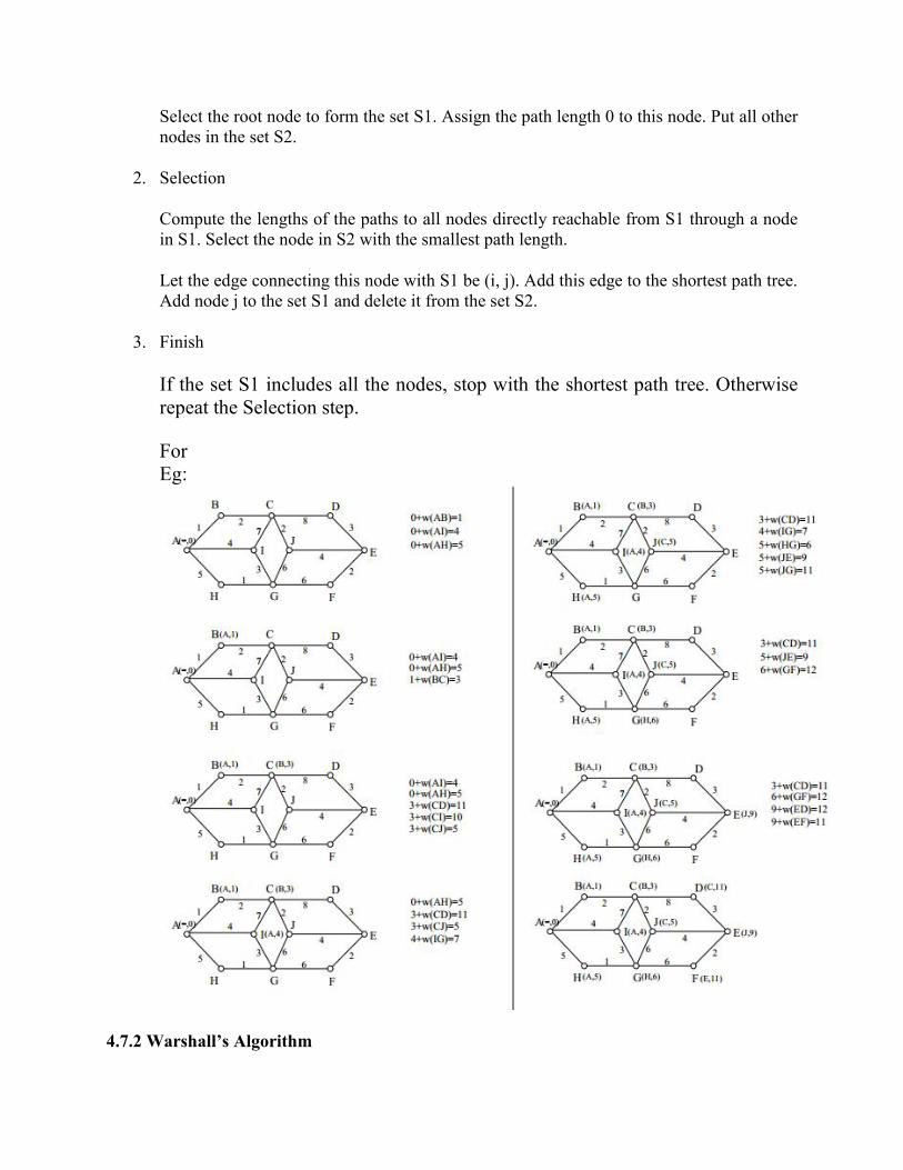
Select the root node to form the set S1. Assign the path length 0 to this node. Put all other nodes in the set S2.

2. Selection

Compute the lengths of the paths to all nodes directly reachable from S1 through a node in S1. Select the node in S2 with the smallest path length.

Let the edge connecting this node with S1 be (i, j). Add this edge to the shortest path tree. Add node j to the set S1 and delete it from the set S2.

3. Finish

If the set S1 includes all the nodes, stop with the shortest path tree. Otherwise repeat the Selection step.

For Eg:

4.7.2 Warshall’s Algorithm

Warshall’s Algorithm is a graph analysis algorithm for finding shortest paths in a weighted graph with positive or negative edge weights (but with no negative cycles, see below) and also for finding transitive closure of a relation R.

Floyd-Warshall algorithm uses a matrix of lengths D0 as its input. If there is an edge between nodes i and j, than the matrix D0 contains its length at the corresponding coordinates. The diagonal of the matrix contains only zeros. If there is no edge between edges i and j, than the position (i,j) contains positive infinity. In other words, the matrix represents lengths of all paths between nodes that does not contain any intermediate node.

In each iteration of Floyd-Warshall algorithm is this matrix recalculated, so it contains lengths of paths among all pairs of nodes using gradually enlarging set of intermediate nodes. The matrix D1, which is created by the first iteration of the procedure, contains paths among all nodes using exactly one (predefined) intermediate node. D2 contains lengths using two predefined intermediate nodes. Finally the matrix Dn uses n intermediate nodes.

This transformation can be described using the following recurrent formula:

For Eg.

4.8 INTRODUCTION TO ACTIVITY NETWORKS

An activity network is a directed graph in which the vertices represent activities and edges represent precedence relation between the tasks. The activity network is also called Activity On Vertex (AOV) network.

Topological sort gives the order in which activities can be performed.

Step 1. choose the node having indegree = 0.

Step 2. remove that node and edges connecting to it.

Step 3. Goto step 1.

Eg:

Topological sort will give the following sequence of activities

B->A->D->C->E

UNIT-5

5.1 SEARCHING 5.1.1 Linear Search

Linear search or sequential search is a method for finding a particular value in a list that consists of checking every one of its elements, one at a time and in sequence, until the desired one is found.

Linear search is the simplest search algorithm; it is a special case of brute-force search. Its worst case cost is proportional to the number of elements in the list; and so is its expected cost, if all list elements are equally likely to be searched for. Therefore, if the list has more than a few elements, other methods (such as binary search or hashing) will be faster, but they also impose additional requirements.

How Linear Search works

Linear search in an array is usually programmed by stepping up an index variable until it reaches the last index. This normally requires two comparisons for each list item: one to check whether the index has reached the end of the array, and another one to check whether the item has the desired value.

Linear Search Algorithm

1. Repeat For J = 1 to N

2. If (ITEM == A[J]) Then

3. Print: ITEM found at location J

4. Return [End of If]

[End of For Loop]

5. If (J > N) Then

6. Print: ITEM doesn’t exist

[End of If]

7. Exit

//CODE int a[10],i,n,m,c=0, x; printf("Enter the size of an array: "); scanf("%d",&n); printf("Enter the elements of the array: "); for(i=0;i<=n-1;i++) scanf("%d",&a[i]); printf("Enter the number to be search: "); scanf("%d",&m); for(i=0;i<=n-1;i++) if(a[i]==m) x=I; c=1; break; if(c==0) printf("The number is not in the list"); else printf("The number is found at location %d", x); Complexity of linear Search Linear search on a list of n elements. In the worst case, the search must visit every element once. This happens when the value being searched for is either the last element in the list, or is not in the list. However, on average, assuming the value searched for is in the list and each list element is equally likely to be the value searched for, the search visits only n/2 elements. In best case the array is already sorted i.e O(1) Algorithm Worst Case Average Case Best Case

Linear Search O(n) O(n) O(1)

5.1.2 Binary Search

A binary search or half-interval search algorithm finds the position of a specified input value (the search "key") within an array sorted by key value. For binary search, the array should be arranged in ascending or descending order. In each step, the algorithm compares the search key value with the key value of the middle element of the array. If the keys match, then a matching element has been found and its index is returned. Otherwise, if the search key is less than the middle element's key, then the algorithm repeats its action on the sub-array to the left of the middle element or, if the search key is greater, on the sub-array to the right. If the remaining array to be searched is empty, then the key cannot be found in the array and a special "not found" indication is returned.

How Binary Search Works

Searching a sorted collection is a common task. A dictionary is a sorted list of word definitions. Given a word, one can find its definition. A telephone book is a sorted list of people's names, addresses, and telephone numbers. Knowing someone's name allows one to quickly find their telephone number and address.

Binary Search Algorithm

1. Set BEG = 1 and END = N

2. Set MID = (BEG + END) / 2

3. Repeat step 4 to 8 While (BEG <= END) and (A[MID] ≠ ITEM)

4. If (ITEM < A[MID]) Then

5. Set END = MID – 1

6. Else

7. Set BEG = MID + 1

[End of If]

8. Set MID = (BEG + END) / 2

9. If (A[MID] == ITEM) Then

10. Print: ITEM exists at location MID

11. Else

12. Print: ITEM doesn’t exist

[End of If]

13. Exit

//CODE

int ar[10],val,mid,low,high,size,i;

clrscr();

printf("\nenter the no.s of elements u wanna input in array\n");

scanf("%d",&size);

for(i=0;i<size;i++)

printf("input the element no %d\n",i+1);

scanf("%d",&ar[i]);

printf("the arry inputed is \n");

for(i=0;i<size;i++)

printf("%d\t",ar[i]);

low=0;

high=size-1;

printf("\ninput the no. u wanna search \n");

scanf("%d",&val);

while(val!=ar[mid]&&high>=low)

mid=(low+high)/2;

if(ar[mid]==val)

printf("value found at %d position",mid+1);

if(val>ar[mid])

low=mid+1;

else

high=mid-1;

Complexity of Binary Search

A binary search halves the number of items to check with each iteration, so locating an item (or determining its absence) takes logarithmic time.

Algorithm Worst Case Average Case Best Case

Binary Search O(nlogn) O(nlogn) O(1)

5.2 INTRODUCTION TO SORTING

Sorting is nothing but storage of data in sorted order, it can be in ascending or descending order. The term Sorting comes into picture with the term Searching. There are so many things in our real life that we need to search, like a particular record in database, roll numbers in merit list, a particular telephone number, any particular page in a book etc. Sorting arranges data in a sequence which makes searching easier. Every record which is going to be sorted will contain one key. Based on the key the record will be sorted. For example, suppose we have a record of students, every such record will have the following data: Roll No. Name Age Here Student roll no. can be taken as key for sorting the records in ascending or descending order. Now suppose we have to search a Student with roll no. 15, we don't need to search the complete record we will simply search between the Students with roll no. 10 to 20. Sorting Efficiency There are many techniques for sorting. Implementation of particular sorting technique depends upon situation. Sorting techniques mainly depends on two parameters. First parameter is the execution time of program, which means time taken for execution of program. Second is the space, which means space taken by the program.

5.3 TYPES OF SORTING • An internal sort is any data sorting process that takes place entirely within the main

memory of a computer. This is possible whenever the data to be sorted is small enough to all be held in the main memory.

• External sorting is a term for a class of sorting algorithms that can handle massive amounts of data. External sorting is required when the data being sorted do not fit into the main memory of a computing device (usually RAM) and instead they must reside in the slower external memory (usually a hard drive). External sorting typically uses a hybrid sort-merge strategy. In the sorting phase, chunks of data small enough to fit in main memory are read, sorted, and written out to a temporary file. In the merge phase, the sorted sub files are combined into a single larger file.

• We can say a sorting algorithm is stable if two objects with equal keys appear in the same order in sorted output as they appear in the input unsorted array.

5.3.1 Insertion sort

It is a simple sorting algorithm that builds the final sorted array (or list) one item at a time. This algorithm is less efficient on large lists than more advanced algorithms such as quicksort, heapsort, or merge sort. However, insertion sort provides several advantages:

• Simple implementation

• Efficient for small data sets • Stable; i.e., does not change the relative order of elements with equal keys • In-place; i.e., only requires a constant amount O(1) of additional memory space.

How Insertion Sort Works

Insertion Sort Algorithm

This algorithm sorts the array A with N elements.

1. Set A[0]=-12345(infinity i.e. Any large no)

2. Repeat step 3 to 5 for k=2 to n

3. Set key=A[k] And j=k-1

4. Repeat while key<A[j]

A) Set A[j+1]=A[j]

b) j=j-1

5. Set A[j+1]=key

6. Return

//CODE

int A[6] = 5, 1, 6, 2, 4, 3; int i, j, key; for(i=1; i<6; i++) key = A[i]; j = i-1; while(j>=0 && key < A[j]) A[j+1] = A[j]; j--; A[j+1] = key; Complexity of Insertion Sort The number f(n) of comparisons in the insertion sort algorithm can be easily computed. First of all, the worst case occurs when the array A is in reverse order and the inner loop must use the maximum number K-1 of comparisons. Hence F(n)= 1+2+3+……………………………….+(n-1)=n(n-1)/2= O(n2) Furthermore, One can show that, on the average, there will be approximately (K-1)/2 comparisons in the inner loop. Accordingly, for the average case. F(n)=O(n2) Thus the insertion sort algorithm is a very slow algorithm when n is very large. Algorithm Worst Case Average Case Best Case

Insertion Sort n(n-1)/2 = O(n2) n(n-1)/4 = O(n2) O(n)

5.3.2 Selection Sort Selection sorting is conceptually the simplest sorting algorithm. This algorithm first finds the smallest element in the array and exchanges it with the element in the first position, then find the second smallest element and exchange it with the element in the second position, and continues in this way until the entire array is sorted How Selection Sort works In the first pass, the smallest element found is 1, so it is placed at the first position, then leaving first element, smallest element is searched from the rest of the elements, 3 is the smallest, so it is then placed at the second position. Then we leave 1 and 3, from the rest of the elements, we search for the smallest and put it at third position and keep doing this, until array is sorted

Selection Sort Algorithm 1. Repeat For J = 0 to N-1 2. Set MIN = J 3. Repeat For K = J+1 to N 4. If (A[K] < A[MIN]) Then 5. Set MIN = K [End of If] [End of Step 3 For Loop] 6. Interchange A[J] and A[MIN] [End of Step 1 For Loop] 7. Exit //CODE void selectionSort(int a[], int size) int i, j, min, temp; for(i=0; i < size-1; i++ ) min = i; //setting min as i for(j=i+1; j < size; j++) if(a[j] < a[min]) //if element at j is less than element at min position min = j; //then set min as j temp = a[i]; a[i] = a[min]; a[min] = temp;

Complexity of Selection Sort Algorithm The number of comparison in the selection sort algorithm is independent of the original order of the element. That is there are n-1 comparison during PASS 1 to find the smallest element, there are n-2 comparisons during PASS 2 to find the second smallest element, and so on. Accordingly F(n)=(n-1)+(n-2)+…………………………+2+1=n(n-1)/2 = O(n2) Algorithm Worst Case Average Case Best Case

Selection Sort n(n-1)/2 = O(n2) n(n-1)/2 = O(n2) O(n2)

5.3.3 Bubble Sort

Bubble Sort is an algorithm which is used to sort N elements that are given in a memory for eg: an Array with N number of elements. Bubble Sort compares all the element one by one and sort them based on their values. It is called Bubble sort, because with each iteration the smaller element in the list bubbles up towards the first place, just like a water bubble rises up to the water surface. Sorting takes place by stepping through all the data items one-by-one in pairs and comparing adjacent data items and swapping each pair that is out of order. How Bubble Sort Works

Let us take the array of numbers "5 1 4 2 8", and sort the array from lowest number to greatest number using bubble sort. In each step, elements written in bold are being compared. Three passes will be required.

First Pass: ( 5 1 4 2 8 ) ( 1 5 4 2 8 ), Here, algorithm compares the first two elements, and swaps since 5 > 1. ( 1 5 4 2 8 ) ( 1 4 5 2 8 ), Swap since 5 > 4 ( 1 4 5 2 8 ) ( 1 4 2 5 8 ), Swap since 5 > 2 ( 1 4 2 5 8 ) ( 1 4 2 5 8 ), Now, since these elements are already in order (8 > 5), algorithm does not swap them.

Second Pass: ( 1 4 2 5 8 ) ( 1 4 2 5 8 ) ( 1 4 2 5 8 ) ( 1 2 4 5 8 ), Swap since 4 > 2 ( 1 2 4 5 8 ) ( 1 2 4 5 8 ) ( 1 2 4 5 8 ) ( 1 2 4 5 8 ) Now, the array is already sorted, but our algorithm does not know if it is completed. The algorithm needs one whole pass without any swap to know it is sorted.

Third Pass: ( 1 2 4 5 8 ) ( 1 2 4 5 8 ) ( 1 2 4 5 8 ) ( 1 2 4 5 8 ) ( 1 2 4 5 8 ) ( 1 2 4 5 8 ) ( 1 2 4 5 8 ) ( 1 2 4 5 8 )

Bubble Sort Algorithm

1. Repeat Step 2 and 3 for k=1 to n

2. Set ptr=1

3. Repeat while ptr<n-k

a) If (A[ptr] > A[ptr+1]) Then

Interchange A[ptr] and A[ptr+1]

[End of If]

b) ptr=ptr+1

[end of step 3 loop]

[end of step 1 loop]

4. Exit

//CODE

Let's consider an array with values 5, 1, 6, 2, 4, 3 int a[6] = 5, 1, 6, 2, 4, 3; int i, j, temp; for(i=0; i<6, i++) for(j=0; j<6-i-1; j++) if( a[j] > a[j+1]) temp = a[j]; a[j] = a[j+1]; a[j+1] = temp;

Above is the algorithm, to sort an array using Bubble Sort. Although the above logic will sort and unsorted array, still the above algorithm isn't efficient and can be enhanced further. Because as per the above logic, the for loop will keep going for six iterations even if the array gets sorted after the second iteration. Hence we can insert a flag and can keep checking whether swapping of elements is taking place or not. If no swapping is taking place that means the array is sorted and we can jump out of the for loop. int a[6] = 5, 1, 6, 2, 4, 3; int i, j, temp; for(i=0; i<6, i++) for(j=0; j<6-i-1; j++) int flag = 0; //taking a flag variable if( a[j] > a[j+1]) temp = a[j]; a[j] = a[j+1]; a[j+1] = temp; flag = 1; //setting flag as 1, if swapping occurs if(!flag) //breaking out of for loop if no swapping takes place break; In the above code, if in a complete single cycle of j iteration(inner for loop), no swapping takes place, and flag remains 0, then we will break out of the for loops, because the array has already been sorted. Complexity of Bubble Sort Algorithm In Bubble Sort, n-1 comparisons will be done in 1st pass, n-2 in 2nd pass, n-3 in 3rd pass and so on. So the total number of comparisons will be F(n)=(n-1)+(n-2)+…………………………+2+1=n(n-1)/2 = O(n2) Algorithm Worst Case Average Case Best Case

Bubble Sort n(n-1)/2 = O(n2) n(n-1)/2 = O(n2) O(n)

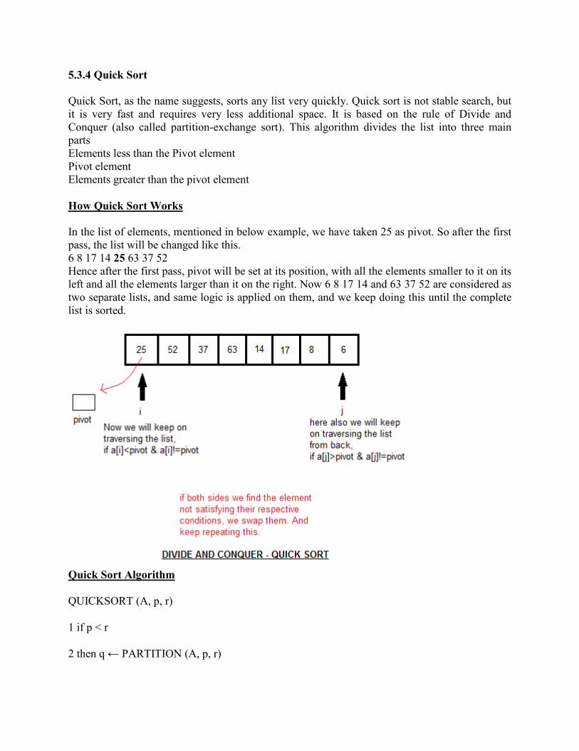
5.3.4 Quick Sort Quick Sort, as the name suggests, sorts any list very quickly. Quick sort is not stable search, but it is very fast and requires very less additional space. It is based on the rule of Divide and Conquer (also called partition-exchange sort). This algorithm divides the list into three main parts Elements less than the Pivot element Pivot element Elements greater than the pivot element How Quick Sort Works In the list of elements, mentioned in below example, we have taken 25 as pivot. So after the first pass, the list will be changed like this. 6 8 17 14 25 63 37 52 Hence after the first pass, pivot will be set at its position, with all the elements smaller to it on its left and all the elements larger than it on the right. Now 6 8 17 14 and 63 37 52 are considered as two separate lists, and same logic is applied on them, and we keep doing this until the complete list is sorted.

Quick Sort Algorithm

QUICKSORT (A, p, r)

1 if p < r

2 then q ← PARTITION (A, p, r)

3 QUICKSORT (A, p, q - 1)

4 QUICKSORT (A, q + 1, r)

The key to the algorithm is the PARTITION procedure, which rearranges the subarray A[p r] in place.

PARTITION (A, p, r)

1 x ← A[r]

2 i ← p - 1

3 for j ← p to r - 1

4 do if A[j] ≤ x

5 then i ← i + 1

6 exchange A[i] ↔ A[j]

7 exchange A[i + 1] ↔ A[r]

8 return i + 1

//CODE

/* Sorting using Quick Sort Algorithm a[] is the array, p is starting index, that is 0, and r is the last index of array. */ void quicksort(int a[], int p, int r) if(p < r) int q; q = partition(a, p, r); quicksort(a, p, q-1); quicksort(a, q+1, r); int partition (int a[], int p, int r) int i, j, pivot, temp; pivot = a[p];

i = p; j = r; while(1) while(a[i] < pivot && a[i] != pivot) i++; while(a[j] > pivot && a[j] != pivot) j--; if(i < j) temp = a[i]; a[i] = a[j]; a[j] = temp; else Return j; Complexity of Quick Sort Algorithm The Worst Case occurs when the list is sorted. Then the first element will require n comparisons to recognize that it remains in the first position. Furthermore, the first sublist will be empty, but the second sublist will have n-1 elements. Accordingly the second element require n-1 comparisons to recognize that it remains in the second position and so on. F(n)= n+(n-1)+(n-2)+…………………………+2+1=n(n+1)/2 = O(n2) Algorithm Worst Case Average Case Best Case

Quick Sort n(n+1)/2 = O(n2) O(n logn) O(n logn)

5.3.5 Merge Sort

Merge Sort follows the rule of Divide and Conquer. But it doesn't divide the list into two halves. In merge sort the unsorted list is divided into N sub lists, each having one element, because a list of one element is considered sorted. Then, it repeatedly merge these sub lists, to produce new sorted sub lists, and at lasts one sorted list is produced. Merge Sort is quite fast, and has a time complexity of O(n log n). It is also a stable sort, which means the equal elements are ordered in the same order in the sorted list.

How Merge Sort Works

Suppose the array A contains 8 elements, each pass of the merge-sort algorithm will start at the beginning of the array A and merge pairs of sorted subarrays as follows.

PASS 1. Merge each pair of elements to obtain the list of sorted pairs.

PASS 2. Merge each pair of pairs to obtain the list of sorted quadruplets.

PASS 3. Merge each pair of sorted quadruplets to obtain the two sorted subarrays.

PASS 4. Merge the two sorted subarrays to obtain the single sorted array.

Merge Sort Algorithm

/* Sorting using Merge Sort Algorithm a[] is the array, p is starting index, that is 0, and r is the last index of array. */ Lets take a[5] = 32, 45, 67, 2, 7 as the array to be sorted. void mergesort(int a[], int p, int r) int q; if(p < r) q = floor( (p+r) / 2); mergesort(a, p, q);

mergesort(a, q+1, r); merge(a, p, q, r); void merge (int a[], int p, int q, int r) int b[5]; //same size of a[] int i, j, k; k = 0; i = p; j = q+1; while(i <= q && j <= r) if(a[i] < a[j]) b[k++] = a[i++]; // same as b[k]=a[i]; k++; i++; else b[k++] = a[j++]; while(i <= q) b[k++] = a[i++]; while(j <= r) b[k++] = a[j++]; for(i=r; i >= p; i--) a[i] = b[--k]; // copying back the sorted list to a[] Complexity of Merge Sort Algorithm Let f(n) denote the number of comparisons needed to sort an n-element array A using merge-sort algorithm. The algorithm requires at most logn passes. Each pass merges a total of n elements and each pass require at most n comparisons. Thus for both the worst and average case

F(n) ≤ n logn Thus the time complexity of Merge Sort is O(n Log n) in all 3 cases (worst, average and best) as merge sort always divides the array in two halves and take linear time to merge two halves. Algorithm Worst Case Average Case Best Case

Merge Sort O(n logn) O(n logn) O(n logn)

5.3.6 Heap Sort Heap Sort is one of the best sorting methods being in-place and with no quadratic worst-case scenarios. Heap sort algorithm is divided into two basic parts Creating a Heap of the unsorted list. Then a sorted array is created by repeatedly removing the largest/smallest element from the heap, and inserting it into the array. The heap is reconstructed after each removal. What is a Heap? Heap is a special tree-based data structure that satisfies the following special heap properties Shape Property: Heap data structure is always a Complete Binary Tree, which means all levels of the tree are fully filled. Heap Property: All nodes are either greater than or equal to or less than or equal to each of its children. If the parent nodes are greater than their children, heap is called a Max-Heap, and if the parent nodes are smaller than their child nodes, heap is called Min-Heap. How Heap Sort Works Initially on receiving an unsorted list, the first step in heap sort is to create a Heap data structure (Max-Heap or Min-Heap). Once heap is built, the first element of the Heap is either largest or smallest (depending upon Max-Heap or Min-Heap), so we put the first element of the heap in our array. Then we again make heap using the remaining elements, to again pick the first element of the heap and put it into the array. We keep on doing the same repeatedly until we have the complete sorted list in our array.

Heap Sort Algorithm

• HEAPSORT(A) 1. BUILD-MAX-HEAP(A) 2. for i ← length[A] downto 2 3. do exchange A[1] ↔ A[i ] 4. heap-size[A] ← heap-size[A] – 1 5. MAX-HEAPIFY(A, 1)

• BUILD-MAX-HEAP(A) 1. heap-size[A] ← length[A] 2. for i ← length[A]/2 downto 1 3. do MAX-HEAPIFY(A, i )

• MAX-HEAPIFY(A, i ) 1. l ← LEFT(i ) 2. r ← RIGHT(i ) 3. if l ≤ heap-size[A] and A[l] > A[i ] 4. then largest ←l 5. else largest ←i 6. if r ≤ heap-size[A] and A[r] > A[largest] 7. then largest ←r 8. if largest = i 9. then exchange A[i ] ↔ A[largest] 10. MAX-HEAPIFY(A, largest)

//CODE In the below algorithm, initially heapsort() function is called, which calls buildmaxheap() to build heap, which inturn uses maxheap() to build the heap. void heapsort(int[], int); void buildmaxheap(int [], int); void maxheap(int [], int, int); void main() int a[10], i, size; printf("Enter size of list"); // less than 10, because max size of array is 10 scanf(“%d”,&size); printf( "Enter" elements"); for( i=0; i < size; i++) Scanf(“%d”,&a[i]); heapsort(a, size); getch(); void heapsort (int a[], int length) buildmaxheap(a, length); int heapsize, i, temp; heapsize = length - 1; for( i=heapsize; i >= 0; i--) temp = a[0]; a[0] = a[heapsize]; a[heapsize] = temp; heapsize--; maxheap(a, 0, heapsize); for( i=0; i < length; i++) Printf("\t%d" ,a[i]); void buildmaxheap (int a[], int length) int i, heapsize; heapsize = length - 1;

for( i=(length/2); i >= 0; i--) maxheap(a, i, heapsize); void maxheap(int a[], int i, int heapsize) int l, r, largest, temp; l = 2*i; r = 2*i + 1; if(l <= heapsize && a[l] > a[i]) largest = l; else largest = i; if( r <= heapsize && a[r] > a[largest]) largest = r; if(largest != i) temp = a[i]; a[i] = a[largest]; a[largest] = temp; maxheap(a, largest, heapsize); Complexity of Heap Sort Algorithm The heap sort algorithm is applied to an array A with n elements. The algorithm has two phases, and we analyze the complexity of each phae separately. Phase 1. Suppose H is a heap. The number of comparisons to find the appropriate place of a new element item in H cannot exceed the depth of H. Since H is complete tree, its depth is bounded by log2m where m is the number of elements in H. Accordingly, the total number g(n) of comparisons to insert the n elements of A into H is bounded as g(n) ≤ n log2n Phase 2. If H is a complete tree with m elements, the left and right subtrees of H are heaps and L is the root of H Reheaping uses 4 comparisons to move the node L one step down the tree H. Since the depth cannot exceeds log2m , it uses 4log2m comparisons to find the appropriate place of L in the tree H. h(n)≤4nlog2n

Thus each phase requires time proportional to nlog2n, the running time to sort n elements array A would be nlog2n Algorithm Worst Case Average Case Best Case

Heap Sort O(n logn) O(n logn) O(n logn)

5.3.7 Radix Sort

The idea is to consider the key one character at a time and to divide the entries, not into two sub lists, but into as many sub lists as there are possibilities for the given character from the key. If our keys, for example, are words or other alphabetic strings, then we divide the list into 26 sub lists at each stage. That is, we set up a table of 26 lists and distribute the entries into the lists according to one of the characters in the key. How Radix Sort Works A person sorting words by this method might first distribute the words into 26 lists according to the initial letter (or distribute punched cards into 12 piles), then divide each of these sub lists into further sub lists according to the second letter, and so on. The following idea eliminates this multiplicity of sub lists: Partition the items into the table of sub lists first by the least significant position, not the most significant. After this first partition, the sub lists from the table are put back together as a single list, in the order given by the character in the least significant position. The list is then partitioned into the table according to the second least significant position and recombined as one list. When, after repetition of these steps, the list has been partitioned by the most significant place and recombined, it will be completely sorted. This process is illustrated by sorting the list of nine three-letter words below.

Radix Sort Algorithm Radixsort(A,d)

1. For i←1 to d 2. Do use a stable sort to sort array A on digit i

Complexity of Radix Sort Algorithm The list A of n elements A1, A2,……………An is given. Let d denote the radix(e.g d=10 for decimal digits, d=26 for letters and d=2 for bits) and each item Ai is represented by means of s of the digits: Ai = di1 di2………………. dis

The radix sort require s passes, the number of digits in each item . Pass K will compare each dik with each of the d digits. Hence C(n)≤ d*s*n Algorithm Worst Case Average Case Best Case

Radix Sort O(n2) d*s*n O(n logn)

5.4 PRACTICAL CONSIDERATION FOR INTERNAL SORTING

Apart from radix sort, all the sorting methods require excessive data movement; i.e., as the result of a comparison, records may be physically moved. This tends to slow down the sorting process when records are large. In sorting files in which the records are large it is necessary to modify the sorting methods so as to minimize data movement. Methods such as Insertion Sort and Merge Sort can be easily modified to work with a linked file rather than a sequential file. In this case each record will require an additional link field. Instead of physically moving the record, its link field will be changed to reflect the change in position of that record in the file. At the end of the sorting process, the records are linked together in the required order. In many applications (e.g., when we just want to sort files and then output them record by record on some external media in the sorted order) this is sufficient. However, in some applications it is necessary to physically rearrange the records in place so that they are in the required order. Even in such cases

considerable savings can be achieved by first performing a linked list sort and then physically rearranging the records according to the order specified in the list. This rearranging can be accomplished in linear time using some additional space.

If the file, F, has been sorted so that at the end of the sort P is a pointer to the first record in a linked list of records then each record in this list will have a key which is greater than or equal to the key of the previous record (if there is a previous record). To physically rearrange these records into the order specified by the list, we begin by interchanging records R1 and RP. Now, the record in the position R1 has the smallest key. If P≠1 then there is some record in the list with link field = 1. If we could change this link field to indicate the new position of the record previously at position 1 then we would be left with records R2, ...,Rn linked together in non decreasing order. Repeating the above process will, after n - 1 iterations, result in the desired rearrangement.

5.5 SEARCH TREES 5.5.1 Binary Search Tree A binary search tree (BST), sometimes also called an ordered or sorted binary tree, is a node based binary tree data structure where each node has a comparable key and satisfies the restriction that the key in any node is larger than the keys in all nodes in that node's left subtree and smaller than the keys in all nodes in that node's right sub-tree. Each node has no more than two child nodes. Each child must either be a leaf node or the root of another binary search tree. The left sub-tree contains only nodes with keys less than the parent node; the right sub-tree contains only nodes with keys greater than the parent node. BSTs are also dynamic data structures, and the size of a BST is only limited by the amount of free memory in the operating system. The main advantage of binary search trees is that it remains ordered, which provides quicker search times than many other data structures. The properties of binary search trees are as follows:

• The left sub tree of a node contains only nodes with keys less than the node's key. • The right subtree of a node contains only nodes with keys greater than the node's key. • The left and right subtree each must also be a binary search tree. • Each node can have up to two successor nodes. • There must be no duplicate nodes. • A unique path exists from the root to every other node.

The major advantage of binary search trees over other data structures is that the related sorting algorithms and search algorithms such as in-order traversal can be very efficient. The other advantages are:

• Binary Search Tree is fast in insertion and deletion etc. when balanced. • Very efficient and its code is easier than other data structures. • Stores keys in the nodes in a way that searching, insertion and deletion can be done

efficiently. • Implementation is very simple in Binary Search Trees. • Nodes in tree are dynamic in nature.

Some of their disadvantages are as follows:

• The shape of the binary search tree totally depends on the order of insertions, and it can be degenerated.

• When inserting or searching for an element in binary search tree, the key of each visited node has to be compared with the key of the element to be inserted or found, i.e., it takes a long time to search an element in a binary search tree.

• The keys in the binary search tree may be long and the run time may increase.

Insertion in BST

Deletion in BST

Consider the BST shown below first the element 4 is deleted. Then 10 is deleted and after that 27 is deleted from the BST.

C program to implement various operations in BST

# include <stdio.h> # include <malloc.h> struct node int info; struct node *lchild; struct node *rchild; *root; main() int choice,num; root=NULL; while(1) printf("\n"); printf("1.Insert\n"); printf("2.Delete\n"); printf("3.Display\n"); printf("4.Quit\n"); printf("Enter your choice : "); scanf("%d",&choice); switch(choice) case 1: printf("Enter the number to be inserted : "); scanf("%d",&num); insert(num); break; case 2: printf("Enter the number to be deleted : "); scanf("%d",&num); del(num); break; case 3: display(root,1); break; case 4: exit(); default: printf("Wrong choice\n"); find(int item,struct node **par,struct node **loc) struct node *ptr,*ptrsave;

if(root==NULL) /*tree empty*/ *loc=NULL; *par=NULL; return; if(item==root->info) /*item is at root*/ *loc=root; *par=NULL; return; if(item<root->info) ptr=root->lchild; else ptr=root->rchild; ptrsave=root; while(ptr!=NULL) if(item==ptr->info) *loc=ptr; *par=ptrsave; return; ptrsave=ptr; if(item<ptr->info) ptr=ptr->lchild; else ptr=ptr->rchild;

*loc=NULL; *par=ptrsave;

insert(int item) struct node *temp,*parent,*location; find(item,&parent,&location); if(location!=NULL) printf("Item already present"); return; temp=(struct node *)malloc(sizeof(struct node));

temp->info=item; temp->lchild=NULL; temp->rchild=NULL; if(parent==NULL) root=temp; else if(item<parent->info) parent->lchild=temp; else parent->rchild=temp;

del(int item) struct node *parent,*location; if(root==NULL) printf("Tree empty"); return; find(item,&parent,&location); if(location==NULL) printf("Item not present in tree"); return; if(location->lchild==NULL && location->rchild==NULL) case_a(parent,location); if(location->lchild!=NULL && location->rchild==NULL) case_b(parent,location); if(location->lchild==NULL && location->rchild!=NULL) case_b(parent,location); if(location->lchild!=NULL && location->rchild!=NULL) case_c(parent,location); free(location);

case_a(struct node *par,struct node *loc ) if(par==NULL) /*item to be deleted is root node*/ root=NULL; else if(loc==par->lchild) par->lchild=NULL; else

par->rchild=NULL;

case_b(struct node *par,struct node *loc) struct node *child; if(loc->lchild!=NULL) /*item to be deleted has lchild */ child=loc->lchild; else child=loc->rchild; if(par==NULL ) /*Item to be deleted is root node*/ root=child; else if( loc==par->lchild) /*item is lchild of its parent*/ par->lchild=child; else /*item is rchild of its parent*/ par->rchild=child; /*End of case_b()*/ case_c(struct node *par,struct node *loc) struct node *ptr,*ptrsave,*suc,*parsuc; /*Find inorder successor and its parent*/ ptrsave=loc; ptr=loc->rchild; while(ptr->lchild!=NULL) ptrsave=ptr; ptr=ptr->lchild; suc=ptr; parsuc=ptrsave; if(suc->lchild==NULL && suc->rchild==NULL) case_a(parsuc,suc); else case_b(parsuc,suc); if(par==NULL) /*if item to be deleted is root node */ root=suc; else if(loc==par->lchild) par->lchild=suc; else par->rchild=suc; suc->lchild=loc->lchild; suc->rchild=loc->rchild; /*End of case_c()*/ display(struct node *ptr,int level

int i; if ( ptr!=NULL ) display(ptr->rchild, level+1); printf("\n"); for (i = 0; i < level; i++) printf(" "); printf("%d", ptr->info); display(ptr->lchild, level+1); /*End of if*/ /*End of display()*/

Complexity of Binary Search Tree

BST Algorithm Average Case Worst Case Insertion O(logn) O(n) Deletion O(logn) O(n)

5.5.2 AVL Trees

An AVL tree (Adelson-Velskii and Landis' tree, named after the inventors) is a self-balancing binary search tree. It was the first such data structure to be invented. In an AVL tree, the heights of the two child subtrees of any node differ by at most one; if at any time they differ by more than one, rebalancing is done to restore this property. Lookup, insertion, and deletion all takeO(log n) time in both the average and worst cases, where n is the number of nodes in the tree prior to the operation. Insertions and deletions may require the tree to be rebalanced by one or more tree rotations.

The balance factor is calculated as follows: balanceFactor = height(left subtree) - height(right subtree). For each node checked, if the balance factor remains −1, 0, or +1 then no rotations are necessary. However, if balance factor becomes less than -1 or greater than +1, the subtree rooted at this node is unbalanced.

In other words,

An AVL tree is a binary search tree which has the following properties:

1. The sub-trees of every node differ in height by at most one. 2. Every sub-tree is an AVL tree.

Insertion To make sure that the given tree remains AVL after every insertion, we must augment the standard BST insert operation to perform some re-balancing. Following are two basic operations that can be performed to re-balance a BST without violating the BST property (keys(left) < key(root)<keys(right)). 1) Left Rotation 2) Right Rotation

T1, T2 and T3 are subtrees of the tree rooted with y (on left side) or x (on right side) y x / \ Right Rotation / \ x T3 – - – - – - – > T1 y / \ < - - - - - - - / \ T1 T2 Left Rotation T2 T3 Keys in both of the above trees follow the following order keys(T1) < key(x) < keys(T2) < key(y) < keys(T3) So BST property is not violated anywhere.

Steps to follow for insertion Let the newly inserted node be w

1)Perform standard BST insert for w. 2) Starting from w, travel up and find the first unbalanced node. Let z be the first unbalanced node, y be the child of z that comes on the path from w to z and x be the grandchild of z that comes on the path from w to z. 3) Re-balance the tree by performing appropriate rotations on the subtree rooted with z. There can be 4 possible cases that needs to be handled as x, y and z can be arranged in 4 ways. Following are the possible 4 arrangements:

a) y is left child of z and x is left child of y (Left Left Case)

b) y is left child of z and x is right child of y (Left Right Case)

c) y is right child of z and x is right child of y (Right Right Case)

d) y is right child of z and x is left child of y (Right Left Case)

Following are the operations to be performed in above mentioned 4 cases. In all of the cases, we only need to re-balance the subtree rooted with z and the complete tree becomes balanced as the height of subtree (After appropriate rotations) rooted with z becomes same as it was before insertion.

a) Left Left Case

T1, T2, T3 and T4 are subtrees.

z y / \ / \ y T4 Right Rotate (z) x z / \ - - - - - - - - -> / \ / \ x T3 T1 T2 T3 T4 / \ T1 T2

b) Left Right Case

z z x / \ / \ / \ y T4 Left Rotate (y) x T4 Right Rotate(z) y z / \ - - - - - - - - -> / \ - - - - - - - -> / \ / \ T1 x y T3 T1 T2 T3 T4 / \ / \ T2 T3 T1 T2 c) Right Right Case z y / \ / \ T1 y Left Rotate(z) z x / \ - - - - - - - -> / \ / \ T2 x T1 T2 T3 T4 / \ T3 T4

d) Right Left Case

z z x / \ / \ / \ T1 y Right Rotate (y) T1 x Left Rotate(z) z y / \ - - - - - - - - -> / \ - - - - - - - -> / \ / \ x T4 T2 y T1 T2 T3 T4 / \ / \ T2 T3 T3 T4

Time Complexity: The rotation operations (left and right rotate) take constant time as only few pointers are being changed there. Updating the height and getting the balance factor also take constant time. So the time complexity of AVL insert remains same as BST insert which is O(h) where h is height of the tree. Since AVL tree is balanced, the height is O(Logn). So time complexity of AVL insert is O(Logn).

Deletion. To make sure that the given tree remains AVL after every deletion, we must augment the standard BST delete operation to perform some re-balancing as described above in insetion.

Let w be the node to be deleted

1) Perform standard BST delete for w.

2) Starting from w, travel up and find the first unbalanced node. Let z be the first unbalanced node, y be the larger height child of z, and x be the larger height child of y. Note that the definitions of x and y are different from insertion here.

3) Re-balance the tree by performing appropriate rotations on the subtree rooted with z as explained above.

Note that, unlike insertion, fixing the node z won’t fix the complete AVL tree. After fixing z, we may have to fix ancestors of z as well.

Time Complexity: The rotation operations (left and right rotate) take constant time as only few pointers are being changed there. Updating the height and getting the balance factor also take constant time. So the time complexity of AVL delete remains same as BST delete which is O(h) where h is height of the tree. Since AVL tree is balanced, the height is O(Logn). So time complexity of AVL delete is O(Logn).For eg:

5.5.3 M-WAY Search Trees

A binary search tree has one value in each node and two subtrees. This notion easily generalizes to an M-way search tree, which has (M-1) values per node and M subtrees. M is called the degree of the tree. A binary search tree, therefore, has degree 2.

In fact, it is not necessary for every node to contain exactly (M-1) values and have exactly M subtrees. In an M-way subtree a node can have anywhere from 1 to (M-1) values, and the number of (non-empty) subtrees can range from 0 (for a leaf) to 1+(the number of values). M is thus a fixed upper limit on how much data can be stored in a node.

The values in a node are stored in ascending order, V1 < V2 < ... Vk (k <= M-1) and the subtrees are placed between adjacent values, with one additional subtree at each end. We can thus associate with each value a `left' and `right' subtree, with the right subtree of Vi being the same as the left subtree of V(i+1). All the values in V1's left subtree are less than V1 , all the values in Vk's subtree are greater than Vk; and all the values in the subtree between V(i) and V(i+1) are greater than V(i) and less than V(i+1).

For example, here is a 3-way search tree:

In the examples it will be convenient to illustrate M-way trees using a small value of M. But in practice, M is usually very large. Each node corresponds to a physical block on disk, and M represents the maximum number of data items that can be stored in a single block.

The algorithm for searching for a value in an M-way search tree is the obvious generalization of the algorithm for searching in a binary search tree. If we are searching for value X and currently at node consisting of values V1...Vk, there are four possible cases that can arise:

1. If X < V1, recursively search for X in V1's left subtree. 2. If X > Vk, recursively search for X in Vk's right subtree. 3. If X=Vi, for some i, then we are done (X has been found). 4. the only remaining possibility is that, for some i, Vi < X < V(i+1). In this case recursively

search for X in the subtree that is in between Vi and V(i+1).

For example, suppose we were searching for 68 in the tree above. At the root, case (2) would apply, so we would continue the search in V2's right subtree. At the root of this subtree, case (4) applies, 68 is between V1=55 and V2=70, so we would continue to search in the subtree between them. Now case (3) applies, 68=V2, so we are done. If we had been searching for 69, exactly the same processing would have occurred down to the last node. At that point, case (2) would apply, but the subtree we want to search in is empty. Therefore we conclude that 69 is not in the tree.

5.5.4 B-trees: Perfectly Height-balanced M-way search trees

A B-tree is an M-way search tree with two special properties:

1. It is perfectly balanced: every leaf node is at the same depth. 2. Every node, except perhaps the root, is at least half-full, i.e. contains M/2 or more values

(of course, it cannot contain more than M-1 values). The root may have any number of values (1 to M-1).

The 3-way search tree above is clearly not a B-tree. Here is a 3-way B-tree containing the same values:

And here is a 5-way B-tree (each node other than the root must contain between 2 and 4 values):

Insertion into a B-Tree

To insert value X into a B-tree, there are 3 steps:

1. using the SEARCH procedure for M-way trees (described above) find the leaf node to which X should be added.

2. add X to this node in the appropriate place among the values already there. Being a leaf node there are no subtrees to worry about.

3. if there are M-1 or fewer values in the node after adding X, then we are finished.

If there are M nodes after adding X, we say the node has overflowed. To repair this, we split the node into three parts:

Left:

the first (M-1)/2 values

Middle:

the middle value (position 1+((M-1)/2)

Right:

the last (M-1)/2 values

For example, let's do a sequence of insertions into this B-tree (M=5, so each node other than the root must contain between 2 and 4 values):

Insert 17: Add it to the middle leaf. No overflow, so we're done.

Insert 6: Add it to the leftmost leaf. That overflows, so we split it:

• Left = [ 2 3 ] • Middle = 5 • Right = [ 6 7 ]

Left and Right become nodes; Middle is added to the node above with Left and Right as its children.

The node above (the root in this small example) does not overflow, so we are done.

Insert 21: Add it to the middle leaf. That overflows, so we split it:

• left = [ 17 21 ] • Middle = 22 • Right = [ 44 45 ]

Left and Right become nodes; Middle is added to the node above with Left and Right as its children.

The node above (the root in this small example) does not overflow, so we are done.

Insert 67: Add it to the rightmost leaf. That overflows, so we split it:

• Left = [ 55 66 ] • Middle = 67 • Right = [ 68 70 ]

Left and Right become nodes; Middle is added to the node above with Left and Right as its children.

But now the node above does overflow. So it is split in exactly the same manner:

• Left = [ 5 10 ] (along with their children) • Middle = 22 • Right = [ 50 67 ] (along with their children)

Left and Right become nodes, the children of Middle. If this were not the root, Middle would be added to the node above and the process repeated. If there is no node above, as in this example, a new root is created with Middle as its only value.

Deleting a Value from a B-Tree

In B-tree if the value to be deleted does not occur in a leaf, we replace it with the largest value in its left subtree and then proceed to delete that value from the node that originally contained it. For example, if we wished to delete 67 from the above tree, we would find the largest value in 67's left subtree, 66, replace 67 with 66, and then delete the occurrence of 66 in the left subtree. In a B-tree, the largest value in any value's left subtree is guaranteed to be in leaf. Therefore wherever the value to be deleted initially resides, the following deletion algorithm always begins at a leaf.

To delete value X from a B-tree, starting at a leaf node, there are 2 steps:

1. Remove X from the current node. Being a leaf node there are no subtrees to worry about. 2. Removing X might cause the node containing it to have too few values.

Remember that we require the root to have at least 1 value in it and all other nodes to have at least (M-1)/2 values in them. If the node has too few values, we say it has underflowed. e.g. deleting 6 from this B-tree (of degree 5):

Removing 6 causes the node it is in to underflow, as it now contains just 1 value (7). Our strategy for fixing this is to try to `borrow' values from a neighbouring node. We join together the current node and its more populous neighbour to form a `combined node' - and we must also include in the combined node the value in the parent node that is in between these two nodes.

In this example, we join node [7] with its more populous neighbour [17 22 44 45] and put `10' in between them, to create

[7 10 17 22 44 45]

How many values might there be in this combined node?

• The parent node contributes 1 value. • The node that underflowed contributes exactly (M-1)/2-1 values. • The neighbouring node contributes somewhere between (M-1)/2 and (M-1) values.

The treatment of the combined node is different depending on whether the neighbouring contributes exactly (M-1)/2 values or more than this number.

Case 1: Suppose that the neighbouring node contains more than (M-1)/2 values. In this case, the total number of values in the combined node is strictly greater than 1 + ((M-1)/2 - 1) + ((M-1)/2), i.e. it is strictly greater than (M-1). So it must contain M values or more.

We split the combined node into three pieces: Left, Middle, and Right, where Middle is a single value in the very middle of the combined node. Because the combined node has M values or more, Left and Right are guaranteed to have (M-1)/2 values each, and therefore are legitimate nodes. We replace the value we borrowed from the parent with Middle and we use Left and Right as its two children. In this case the parent's size does not change, so we are completely finished.

This is what happens in our example of deleting 6 from the tree above. The combined node [7 10 17 22 44 45] contains more than 5 values, so we split it into:

• Left = [ 7 10 ] • Middle = 17 • Right = [ 22 44 45 ]

Then put Middle into the parent node (in the position where the `10' had been) with Left and Right as its children

Case 2: Suppose, on the other hand, that the neighbouring node contains exactly (M-1)/2 values. Then the total number of values in the combined node is 1 + ((M-1)/2 - 1) + ((M-1)/2) = (M-1)

In this case the combined node contains the right number of values to be treated as a node. So we make it into a node and remove from the parent node the value that has been incorporated into

the new, combined node. As a concrete example of this case, suppose that, in the above tree, we had deleted 3 instead of 6. The node [2 3] underflows when 3 is removed. It would be combined with its more populous neighbour [6 7] and the intervening value from the parent (5) to create the combined node [2 5 6 7]. This contains 4 values, so it can be used without further processing. The result would be:

It is very important to note that the parent node now has one fewer value. This might cause it to underflow - imagine that 5 had been the only value in the parent node. If the parent node underflows, it would be treated in exactly the same way - combined with its more populous neighbor etc. The underflow processing repeats at successive levels until no underflow occurs or until the root underflows.

Now let us consider the root. For the root to underflow, it must have originally contained just one value, which now has been removed. If the root was also a leaf, then there is no problem: in this case the tree has become completely empty.

If the root is not a leaf, it must originally have had two subtrees (because it originally contained one value).The deletion process always starts at a leaf and therefore the only way the root could have its value removed is through the Case 2. The root's two children have been combined, along with the root's only value to form a single node. But if the root's two children are now a single node, then that node can be used as the new root, and the current root (which has underflowed) can simply be deleted.

suppose we delete 7 from this B-tree (M=5):

The node [3 7] would underflow, and the combined node [3 10 18 20] would be created. This has 4 values, which is acceptable when M=5. So it would be kept as a node, and `10' would be removed from the parent node - the root. This is the only circumstance in which underflow can occur in a root that is not a leaf. The situation is this:

Clearly, the current root node, now empty, can be deleted and its child used as the new root

5.5.5 B+ Tree

A B+ tree is an n-ary tree with a variable but often large number of children per node. A B+ tree consists of a root, internal nodes and leaves. The root may be either a leaf or a node with two or more children. A B+ tree can be viewed as a B-tree in which each node contains only keys (not key-value pairs), and to which an additional level is added at the bottom with linked leaves.

The primary value of a B+ tree is in storing data for efficient retrieval in a block-oriented storage context — in particular, file systems. This is primarily because unlike binary search trees, B+ trees have very high fanout (number of pointers to child nodes in a node, typically on the order of 100 or more), which reduces the number of I/O operations required to find an element in the tree.

5.6 HASHING

5.6.1 Hash Function

A hash function is a function that:

1. When applied to an Object, returns a number 2. When applied to equal Objects, returns the same number for each 3. When applied to unequal Objects, is very unlikely to return the same number for

each.

Suppose we were to come up with a “magic function” that, given a value to search for, would tell us exactly where in the array to look

1. If it’s in that location, it’s in the array 2. If it’s not in that location, it’s not in the array

A hash function is a function that makes hash of its inputs.Suppose our hash function gave us the following values:

hashCode("apple") = 5 hashCode("watermelon") = 3 hashCode("grapes") = 8 hashCode("cantaloupe") = 7 hashCode("kiwi") = 0

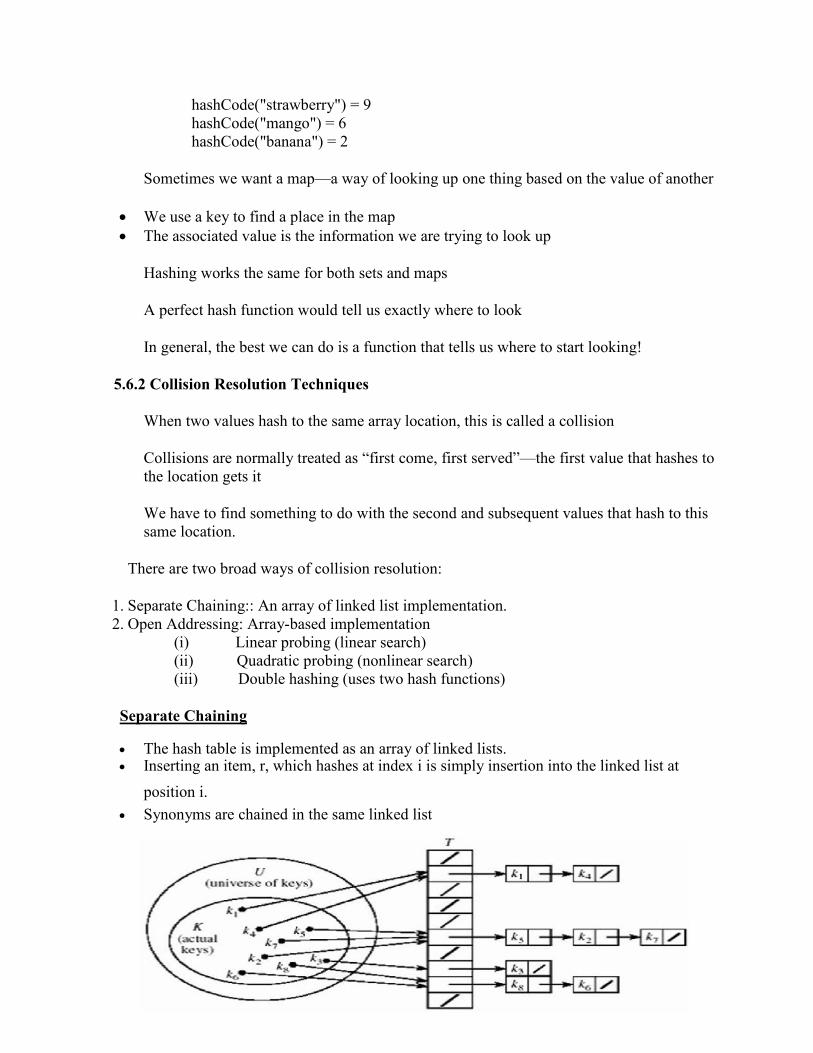
hashCode("strawberry") = 9 hashCode("mango") = 6 hashCode("banana") = 2

Sometimes we want a map—a way of looking up one thing based on the value of another

• We use a key to find a place in the map • The associated value is the information we are trying to look up

Hashing works the same for both sets and maps

A perfect hash function would tell us exactly where to look

In general, the best we can do is a function that tells us where to start looking!

5.6.2 Collision Resolution Techniques

When two values hash to the same array location, this is called a collision

Collisions are normally treated as “first come, first served”—the first value that hashes to the location gets it

We have to find something to do with the second and subsequent values that hash to this same location.

There are two broad ways of collision resolution:

1. Separate Chaining:: An array of linked list implementation. 2. Open Addressing: Array-based implementation

(i) Linear probing (linear search) (ii) Quadratic probing (nonlinear search) (iii) Double hashing (uses two hash functions)

Separate Chaining

• The hash table is implemented as an array of linked lists. • Inserting an item, r, which hashes at index i is simply insertion into the linked list at

position i. • Synonyms are chained in the same linked list

• Retrieval of an item, r, with hash address, i, is simply retrieval from the linked list at position i.

• Deletion of an item, r, with hash address, i, is simply deleting r from the linked list at position i Example: Load the keys 23, 13, 21, 14, 7, 8, and 15 , in this order, in a hash table of size 7 using separate chaining with the hash function: h(key) = key % 7

h(23) = 23 % 7 = 2 h(13) = 13 % 7 = 6 h(21) = 21 % 7 = 0 h(14) = 14 % 7 = 0 collision h(7) = 7 % 7 = 0 collision h(8) = 8 % 7 = 1 h(15) = 15 % 7 = 1 collision

Separate Chaining with String Keys

i) Recall that search keys can be numbers, strings or some other object. ii) A hash function for a string s = c0c1c2…cn-1 can be defined as: iii) hash = (c0 + c1 + c2 + … + cn-1) % tableSize

Separate Chaining with String Keys

Use the hash function hash to load the following commodity items into a hash table of size 13 using separate chaining:

Onion 1 10.0Tomato 1 8.50Cabbage 3 3.50Carrot 1 5.50Okra 1 6.50Mellon 2 10.0

Potato 2 7.50Banana 3 4.00Olive 2 15.0Salt 2 2.50Cucumber 3 4.50Mushroom 3 5.50

Orange 2 3.00Solution:

hash(onion) = (111 + 110 + 105 + 111 + 110) % 13 = 547 % 13 = 1 Separate Chaining versus Open-addressing

Separate chaining has certain advantages over open addressing

i) Collision resolution is simple and efficient. ii) The hash table can hold more elements without the large performance

deterioration of open addressing (The load factor can be 1 or greater) iii) The performance of chaining declines much more slowly than open addressing iv) Deletion is easy - no special flag values are necessary v) Table size need not be a prime number vi) The keys of the objects to be hashed need not be unique

Disadvantage of Separate Chaining

i) It requires the implementation of a separate data structure for chains, and code to manage it.

ii) The main cost of chaining is the extra space required for the linked lists

Open Addressing • All items are stored in the hash table itself • In addition to the cell data (if any), each cell keeps one of the three states: EMPTY.

OCCUPIED, DELETED • While inserting, if a collision occurs, alternative cells are tried until an empty cell is

found. • Deletion: (lazy deletion): When a key is deleted the slot is marked as DELETED rather

than EMPTY otherwise subsequent searches that hash at the deleted cell will fail. • Probe sequence: A probe sequence is the sequence of array indexes that is followed in

searching for an empty cell during an insertion, or in searching for a key during find or delete operations.

• The most common probe sequences are of the form:

hi(key) = [h(key) + c(i)] % n, for i = 0, 1, …, n-1. where h is a

hash function and n is the size of the hash table

The function c(i) is required to have the following two properties: • Property 1: c(0) = 0 • Property 2: The set of values c(0) % n, c(1) % n, c(2) % n, . . . , c(n-1) % n must be a

permutation of 0, 1, 2,. . ., n – 1, that is, it must contain every integer between 0 and n - 1 inclusive

• The function c(i) is used to resolve collisions. • To insert item r, we examine array location h0(r) = h(r). If there is a collision, array

locations h1(r), h2(r), ..., hn-1(r) are examined until an empty slot is found • Similarly, to find item r, we examine the same sequence of locations in the same order. • Note: For a given hash function h(key), the only difference in the open addressing

collision resolution techniques (linear probing, quadratic probing and double hashing) is in the definition of the function c(i).

• Common definitions of c(i) are: Collision Resolution Technique C(i)

Linear Probing I

Quadratic Probing ±i2

Double Hashing i*hp(key)

where hp(key) is another hash function. Table size= smallest prime ≥ number of items in table/ desired load factor

Open Addressing: Linear Probing • c(i) is a linear function in i of the form c(i) = a*i. • Usually c(i) is chosen as:

c(i) = i for i = 0, 1, . . . , tableSize – 1 • The probe sequences are then given by:

hi(key) = [h(key) + i] % tableSize for i = 0, 1, . . . , tableSize – 1

For c(i) = a*i to satisfy Property 2, a and n must be relatively prime.

e.g. Perform the operations given below, in the given order, on an initially empty hash table of size 13 using linear probing with c(i) = i and the hash function: h(key) = key % 13

insert(18), insert(26), insert(35), insert(9), find(15), find(48), delete(35), delete(40), find(9), insert(64), insert(47), find(35) The required probe sequences are given by

hi(key) = (h(key) + i) % 13 i = 0, 1, 2, . . ., 12

Disadvantage of Linear Probing: Primary Clustering

• Linear probing is subject to a primary clustering phenomenon

• Elements tend to cluster around table locations that they originally hash to

• Primary clusters can combine to form larger clusters. This leads to long probe sequences and hence deterioration in hash table efficiency.

5.7 STORAGE MANAGEMENT

5.7.1Garbage Collection

Garbage collection (GC) is a form of automatic memory management. The garbage collector attempts to reclaim garbage, or memory occupied by objects that are no longer in use by the program.

Garbage collection is the opposite of manual memory management, which requires the programmer to specify which objects to deallocate and return to the memory system. Like other memory management techniques, garbage collection may take a significant proportion of total processing time in a program and can thus have significant influence on performance.

Resources other than memory, such as network sockets, database handles, user interaction windows, and file and device descriptors, are not typically handled by garbage collection. Methods used to manage such resources, particularly destructors, may suffice to manage memory as well, leaving no need for GC. Some GC systems allow such other resources to be associated with a region of memory that, when collected, causes the other resource to be reclaimed; this is called finalization. The basic principles of garbage collection are:

• Find data objects in a program that cannot be accessed in the future. • Reclaim the resources used by those objects.

Many programming languages require garbage collection, either as part of the language specification or effectively for practical implementation these are said to be garbage collected languages. Other languages were designed for use with manual memory management, but have garbage collected implementations available (for example, C, C++). While integrating garbage collection into the language's compiler and runtime system enables a much wider choice of methods. The garbage collector will almost always be closely integrated with the memory allocator.

Advantages

Garbage collection frees the programmer from manually dealing with memory deallocation. As a result, certain categories of bugs are eliminated or substantially reduced:

• Dangling pointer bugs, which occur when a piece of memory is freed while there are still pointers to it, and one of those pointers is dereferenced. By then the memory may have been reassigned to another use, with unpredictable results.

• Double free bugs, which occur when the program tries to free a region of memory that has already been freed, and perhaps already been allocated again.

• Certain kinds of memory leaks, in which a program fails to free memory occupied by objects that have become unreachable, which can lead to memory exhaustion.

• Efficient implementations of persistent data structures

Disadvantages

Typically, garbage collection has certain disadvantages:

• Garbage collection consumes computing resources in deciding which memory to free, even though the programmer may have already known this information. The penalty for the convenience of not annotating object lifetime manually in the source code is overhead, which can lead to decreased or uneven performance. Interaction with memory hierarchy effects can make this overhead intolerable in circumstances that are hard to predict or to detect in routine testing.

• The moment when the garbage is actually collected can be unpredictable, resulting in stalls scattered throughout a session. Unpredictable stalls can be unacceptable in real-time environments, in transaction processing, or in interactive programs.

5.7.2 Compaction

The process of moving all marked nodes to one end of memory and all available memory to other end is called compaction. Algorithm which performs compaction is called compacting algorithm. After repeated allocation and de allocation of blocks, the memory becomes fragmented. Compaction is a technique that joins the non contiguous free memory blocks to form one large block so that the total free memory becomes contiguous. All the memory blocks that are in use are moved towards the beginning of the memory i.e. these blocks are copied into sequential locations in the lower portion of the memory. When compaction is performed, all the user programs come to a halt. A problem can arise if any of the used blocks that are copied contain a pointer value. Eg. Suppose inside block P5, the location 350 contains address 310. After compaction the block P5 is moved from location 290 to location 120, so now the pointer value 310 stored inside P5 should change to 140. So after compaction the pointer values inside blocks should be identified and changed accordingly.