Binary Trees, Binary Search Trees

www.cs.ust.hk/~huamin/COMP171/bst.ppt

Trees

•  Linear access time of linked lists is prohibitive – Does there exist any simple data structure

for which the running time of most operations (search, insert, delete) is O(log N)?

Trees

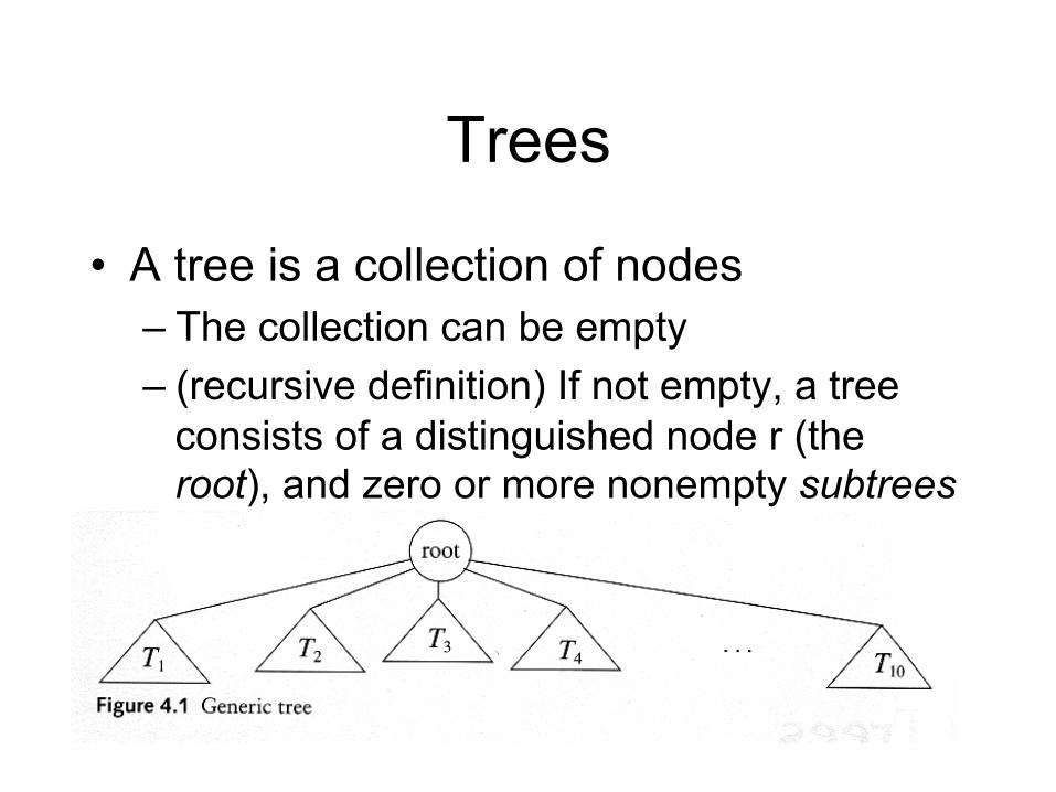
•  A tree is a collection of nodes – The collection can be empty –  (recursive definition) If not empty, a tree

consists of a distinguished node r (the root), and zero or more nonempty subtrees T1, T2, ...., Tk, each of whose roots are connected by a directed edge from r

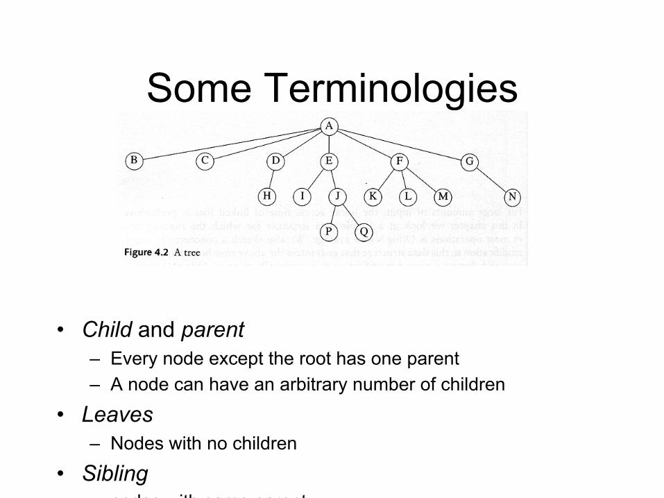
Some Terminologies

•  Child and parent –  Every node except the root has one parent –  A node can have an arbitrary number of children

•  Leaves –  Nodes with no children

•  Sibling –  nodes with same parent

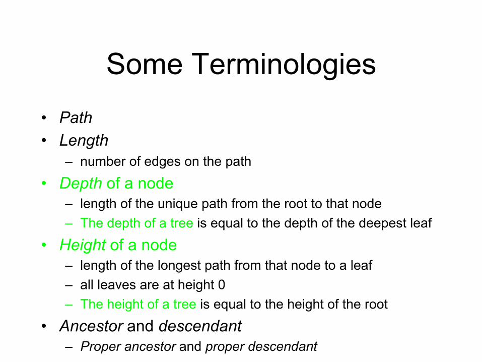
Some Terminologies •  Path •  Length

–  number of edges on the path

•  Depth of a node –  length of the unique path from the root to that node –  The depth of a tree is equal to the depth of the deepest leaf

•  Height of a node –  length of the longest path from that node to a leaf –  all leaves are at height 0 –  The height of a tree is equal to the height of the root

•  Ancestor and descendant –  Proper ancestor and proper descendant

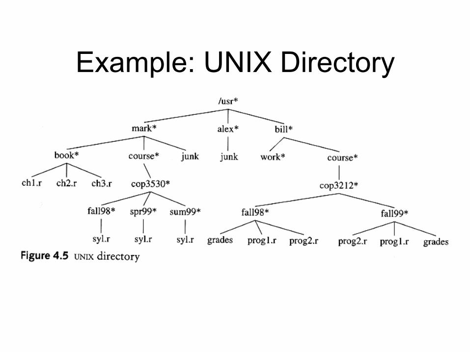
Example: UNIX Directory

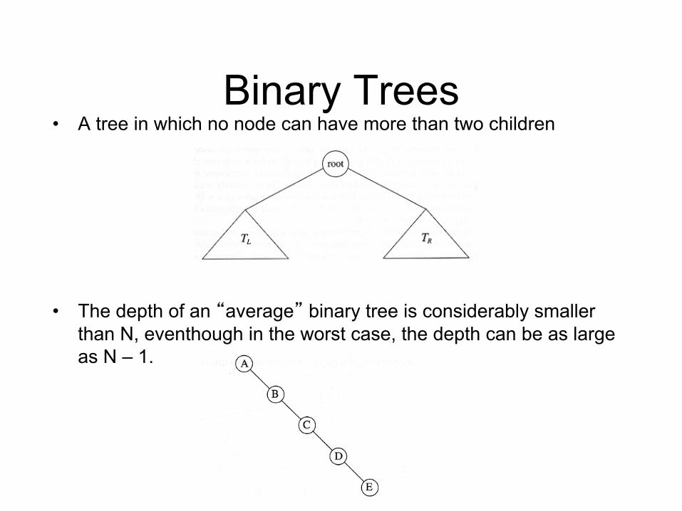
Binary Trees •  A tree in which no node can have more than two children

•  The depth of an “average” binary tree is considerably smaller than N, eventhough in the worst case, the depth can be as large as N – 1.

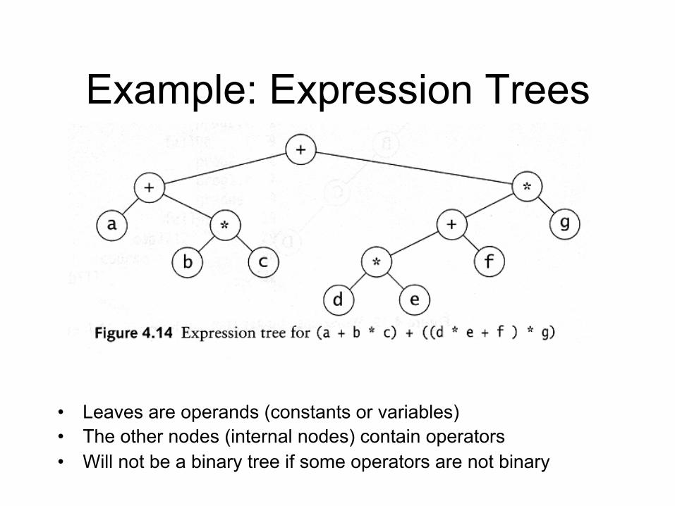
Example: Expression Trees

•  Leaves are operands (constants or variables) •  The other nodes (internal nodes) contain operators •  Will not be a binary tree if some operators are not binary

Tree traversal

•  Used to print out the data in a tree in a certain order

•  Pre-order traversal – Print the data at the root – Recursively print out all data in the left

subtree – Recursively print out all data in the right

subtree

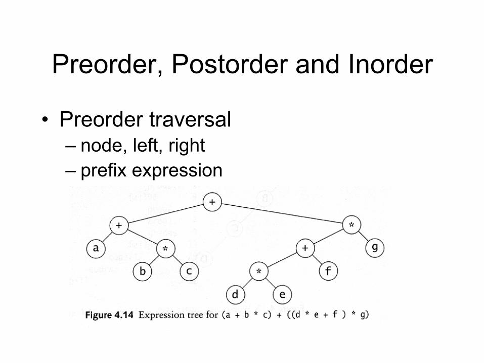
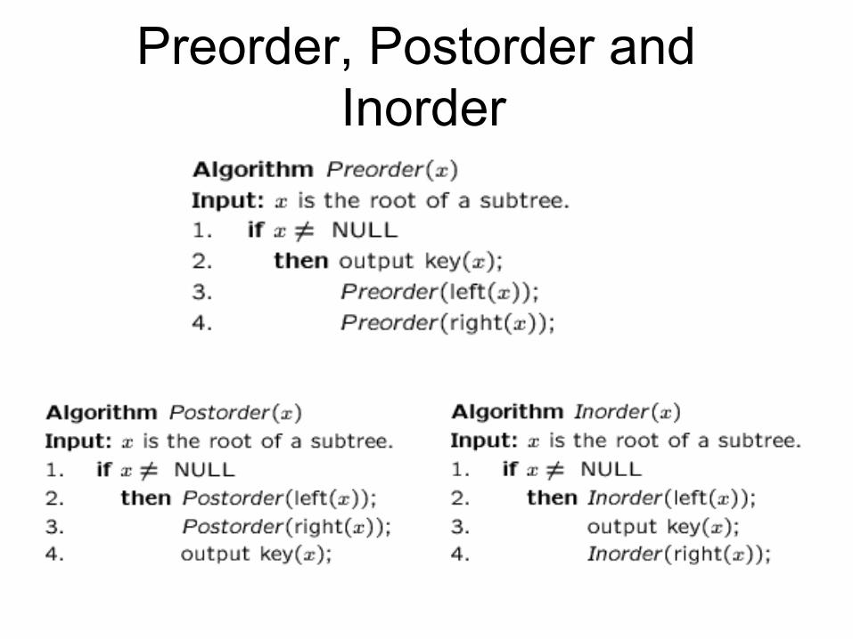
Preorder, Postorder and Inorder

•  Preorder traversal – node, left, right – prefix expression

•  ++a*bc*+*defg

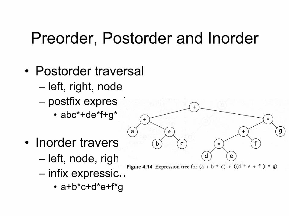
Preorder, Postorder and Inorder

•  Postorder traversal –  left, right, node – postfix expression

•  abc*+de*f+g*+

•  Inorder traversal –  left, node, right. –  infix expression

•  a+b*c+d*e+f*g

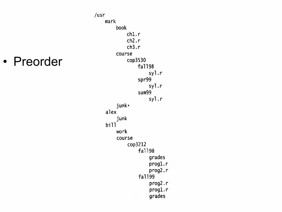
•  Preorder

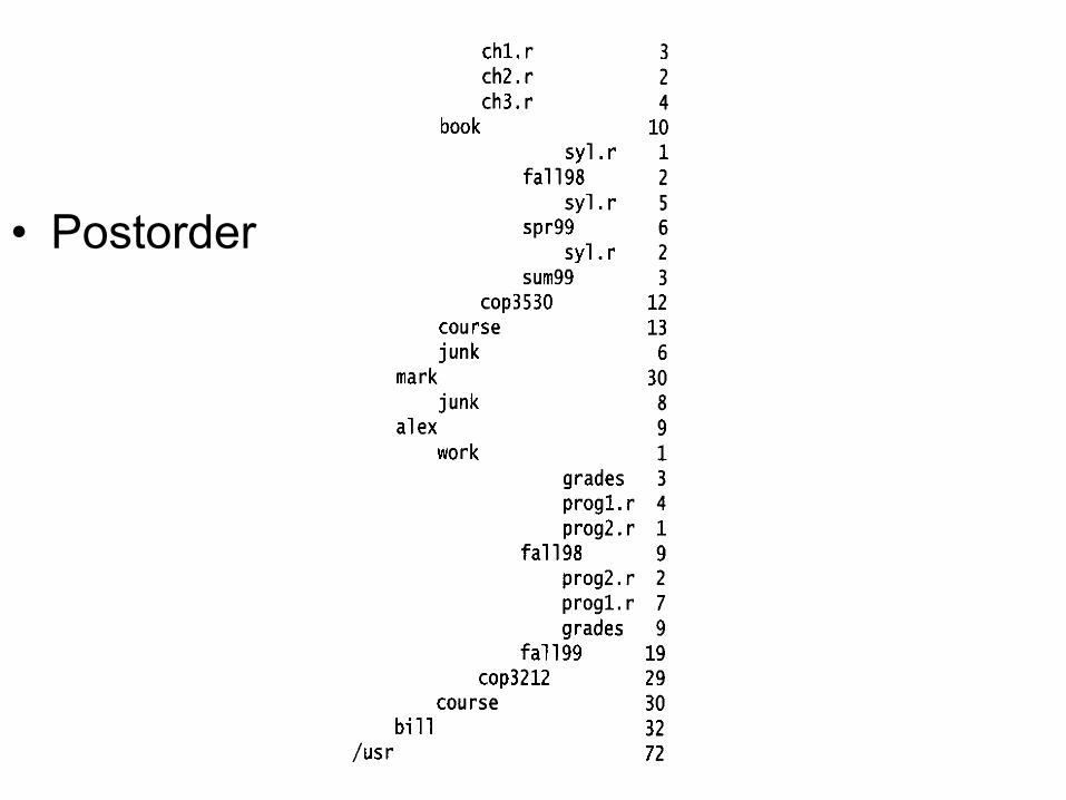
•  Postorder

Preorder, Postorder and Inorder

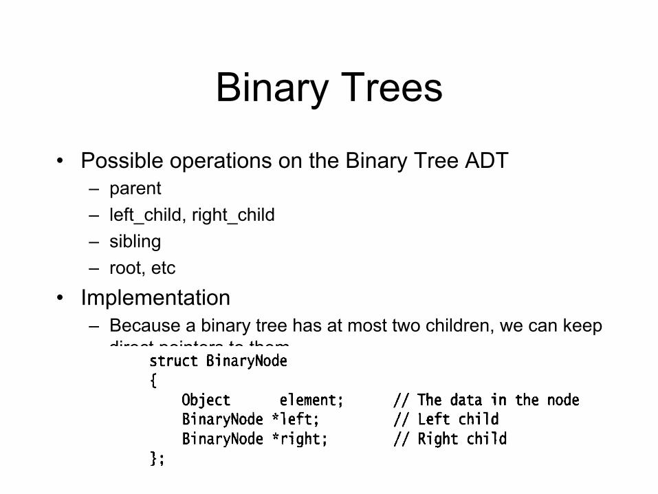
Binary Trees •  Possible operations on the Binary Tree ADT

–  parent –  left_child, right_child –  sibling –  root, etc

•  Implementation –  Because a binary tree has at most two children, we can keep

direct pointers to them

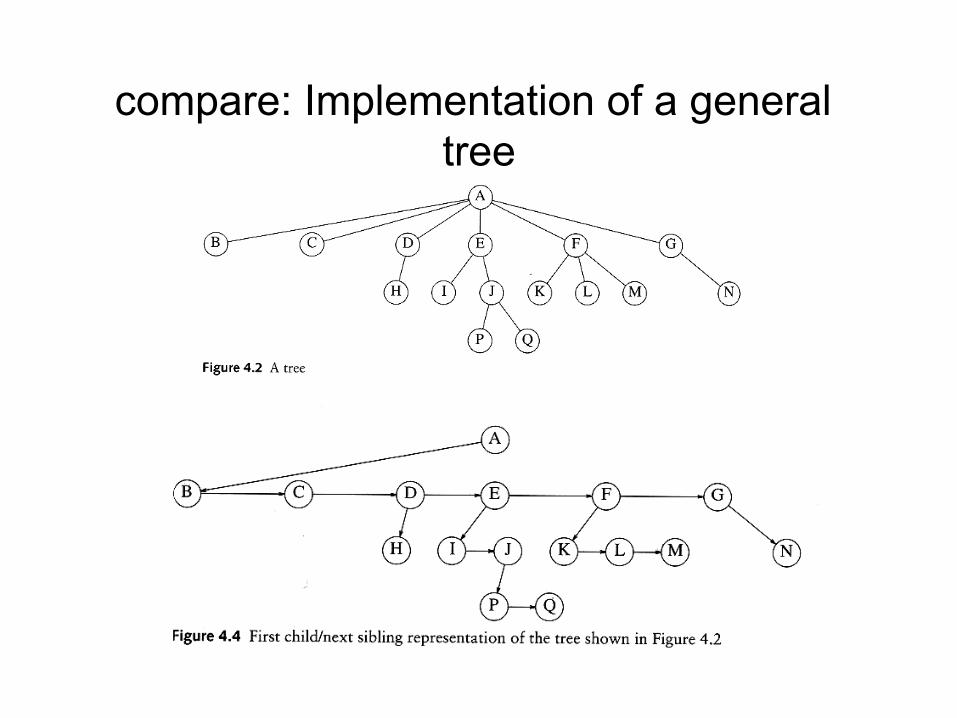
compare: Implementation of a general tree

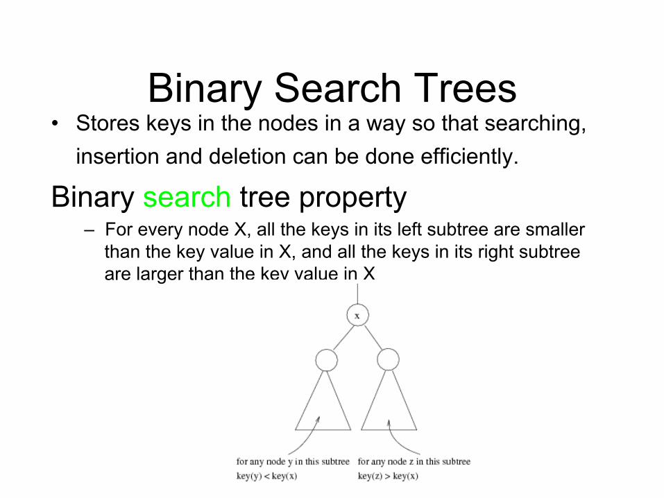
Binary Search Trees •  Stores keys in the nodes in a way so that searching,

insertion and deletion can be done efficiently. Binary search tree property

–  For every node X, all the keys in its left subtree are smaller than the key value in X, and all the keys in its right subtree are larger than the key value in X

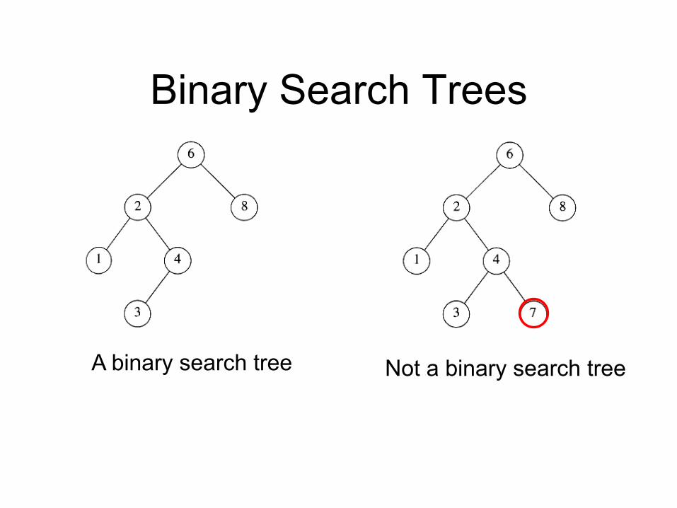
Binary Search Trees

A binary search tree Not a binary search tree

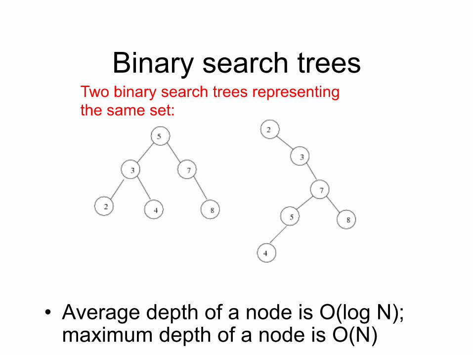
Binary search trees

•  Average depth of a node is O(log N); maximum depth of a node is O(N)

Two binary search trees representing the same set:

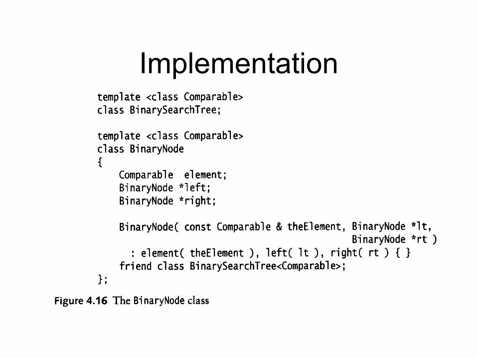
Implementation

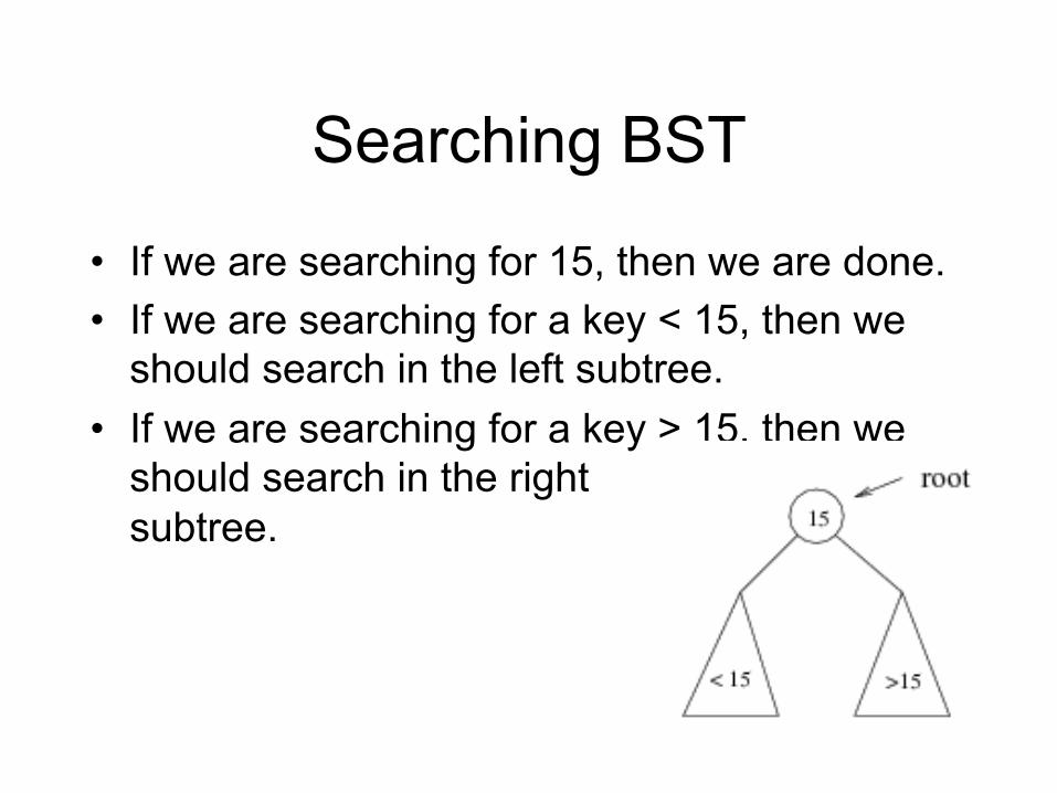
Searching BST

•  If we are searching for 15, then we are done. •  If we are searching for a key < 15, then we

should search in the left subtree. •  If we are searching for a key > 15, then we

should search in the right subtree.

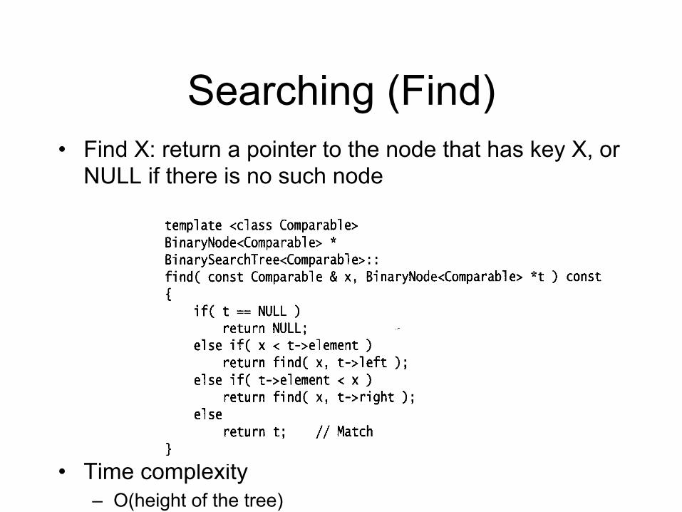
Searching (Find) •  Find X: return a pointer to the node that has key X, or

NULL if there is no such node

•  Time complexity –  O(height of the tree)

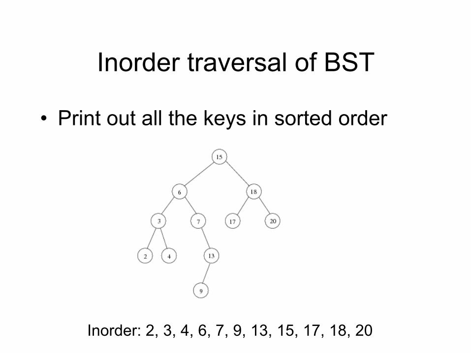
Inorder traversal of BST

•  Print out all the keys in sorted order

Inorder: 2, 3, 4, 6, 7, 9, 13, 15, 17, 18, 20

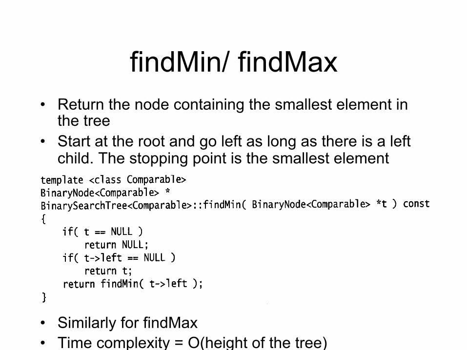
findMin/ findMax •  Return the node containing the smallest element in

the tree •  Start at the root and go left as long as there is a left

child. The stopping point is the smallest element

•  Similarly for findMax •  Time complexity = O(height of the tree)

insert •  Proceed down the tree as you would with a find •  If X is found, do nothing (or update something) •  Otherwise, insert X at the last spot on the path traversed

•  Time complexity = O(height of the tree)

delete

•  When we delete a node, we need to consider how we take care of the children of the deleted node. – This has to be done such that the property

of the search tree is maintained.

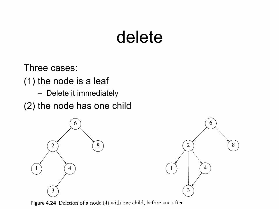
delete Three cases: (1) the node is a leaf

–  Delete it immediately

(2) the node has one child –  Adjust a pointer from the parent to bypass that node

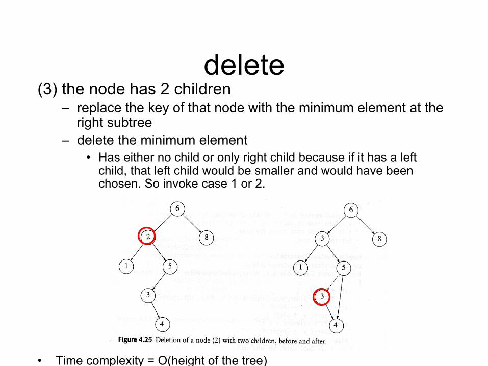
delete (3) the node has 2 children

–  replace the key of that node with the minimum element at the right subtree

–  delete the minimum element •  Has either no child or only right child because if it has a left

child, that left child would be smaller and would have been chosen. So invoke case 1 or 2.

•  Time complexity = O(height of the tree)

30

Priority Queues – Binary Heaps

homes.cs.washington.edu/~anderson/iucee/Slides_326.../

Heaps.ppt

31

Recall Queues

•  FIFO: First-In, First-Out

•  Some contexts where this seems right?

•  Some contexts where some things should be allowed to skip ahead in the line?

32

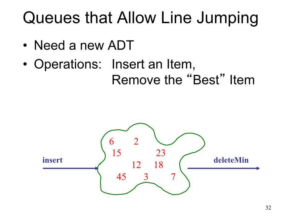
Queues that Allow Line Jumping •  Need a new ADT •  Operations: Insert an Item,

Remove the “Best” Item

insert deleteMin

6 2 15 23 12 18 45 3 7

33

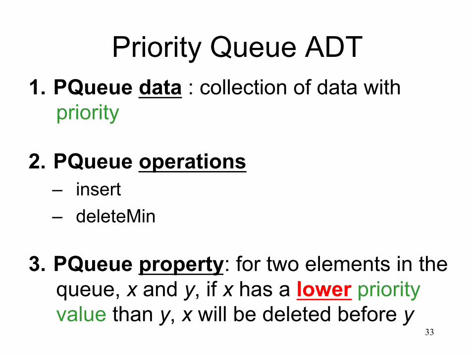
Priority Queue ADT 1.  PQueue data : collection of data with

priority

2.  PQueue operations –  insert –  deleteMin

3.  PQueue property: for two elements in the queue, x and y, if x has a lower priority value than y, x will be deleted before y

34

Applications of the Priority Queue

•  Select print jobs in order of decreasing length •  Forward packets on routers in order of

urgency •  Select most frequent symbols for compression •  Sort numbers, picking minimum first

•  Anything greedy

35

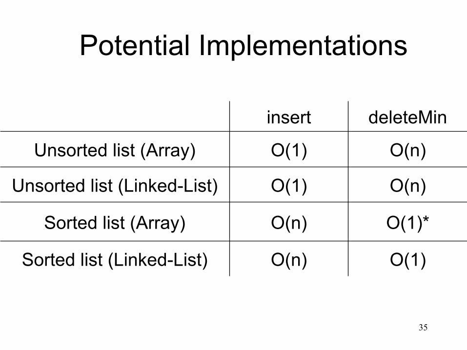
Potential Implementations

insert deleteMin

Unsorted list (Array) O(1) O(n)

Unsorted list (Linked-List) O(1) O(n)

Sorted list (Array) O(n) O(1)*

Sorted list (Linked-List) O(n) O(1)

36

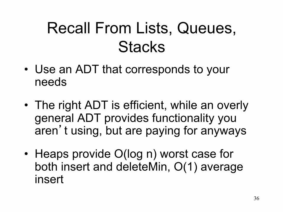
Recall From Lists, Queues, Stacks

•  Use an ADT that corresponds to your needs

•  The right ADT is efficient, while an overly general ADT provides functionality you aren’t using, but are paying for anyways

•  Heaps provide O(log n) worst case for both insert and deleteMin, O(1) average insert

37

Binary Heap Properties

1.  Structure Property 2.  Ordering Property

38

Tree Review A

E

B

D F

C

G

I H

L J M K N

root(T): leaves(T): children(B): parent(H): siblings(E): ancestors(F): descendents(G): subtree(C):

Tree T

39

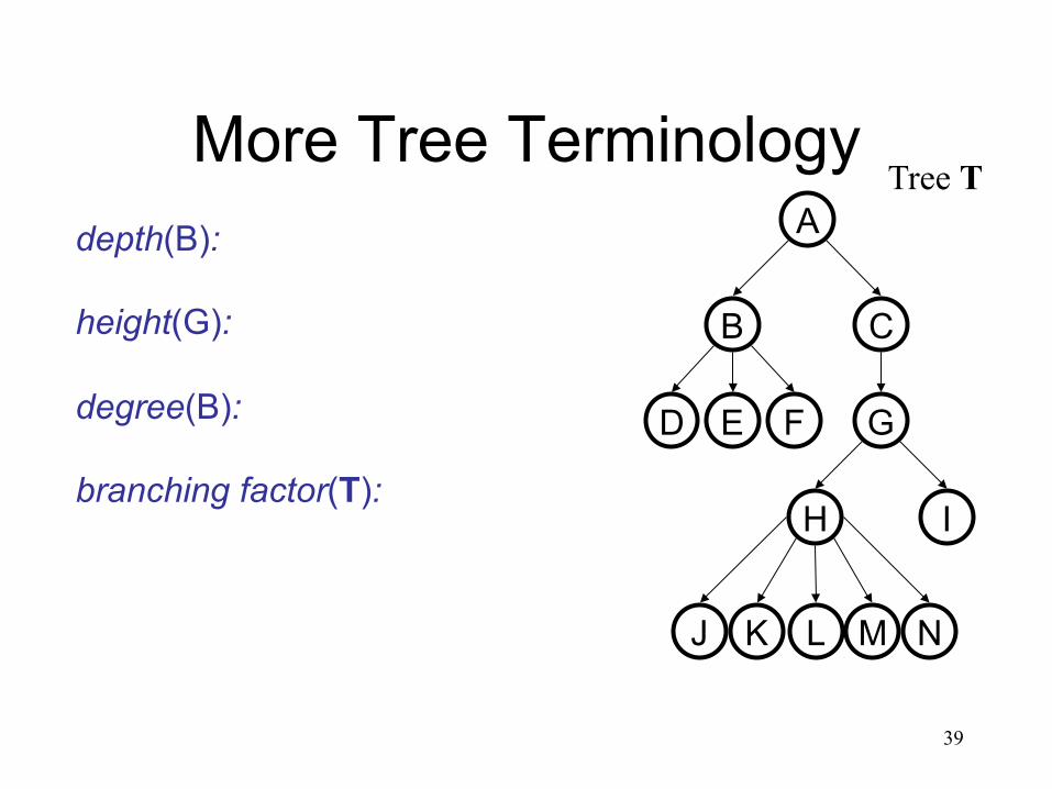
More Tree Terminology A

E

B

D F

C

G

I H

L J M K N

depth(B): height(G): degree(B): branching factor(T):

Tree T

40

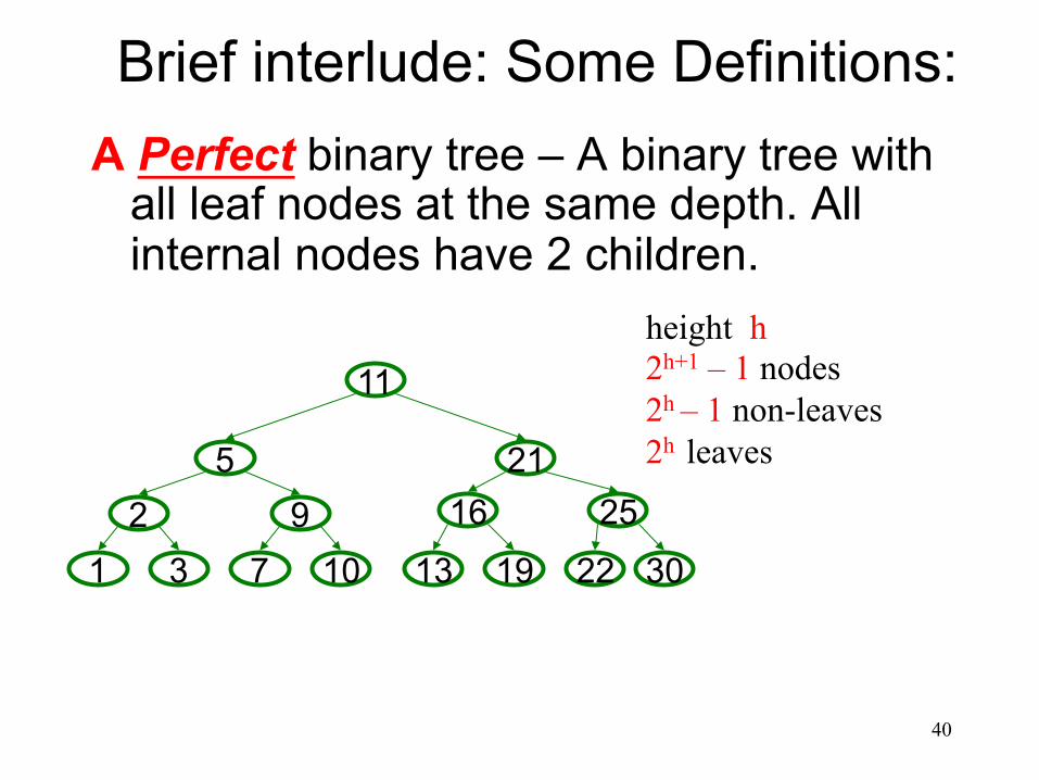
Brief interlude: Some Definitions: A Perfect binary tree – A binary tree with

all leaf nodes at the same depth. All internal nodes have 2 children.

25 9 2 21 5

11

30 7 10 1 3

16

13 19 22

height h 2h+1 – 1 nodes 2h – 1 non-leaves 2h leaves

41

Heap Structure Property •  A binary heap is a complete binary tree. Complete binary tree – binary tree that is

completely filled, with the possible exception of the bottom level, which is filled left to right.

Examples:

42

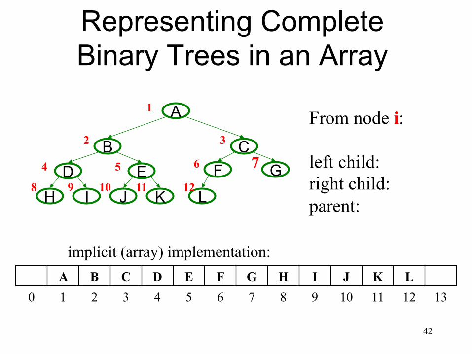
Representing Complete Binary Trees in an Array

G E D C B

A

J K H I

F

L

From node i: left child: right child: parent:

7

1

2 3

4 5 6

9 8 10 11 12

A B C D E F G H I J K L 0 1 2 3 4 5 6 7 8 9 10 11 12 13

implicit (array) implementation:

43

Why this approach to storage?

44

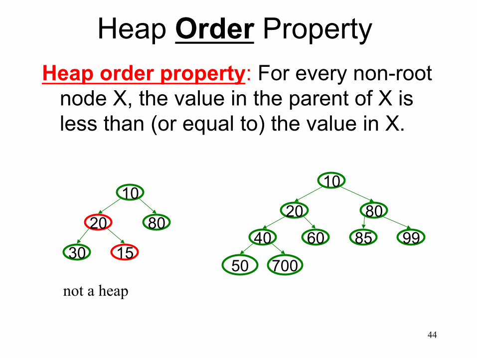
Heap Order Property Heap order property: For every non-root

node X, the value in the parent of X is less than (or equal to) the value in X.

15 30

80 20

10

99 60 40

80 20

10

50 700

85

not a heap

45

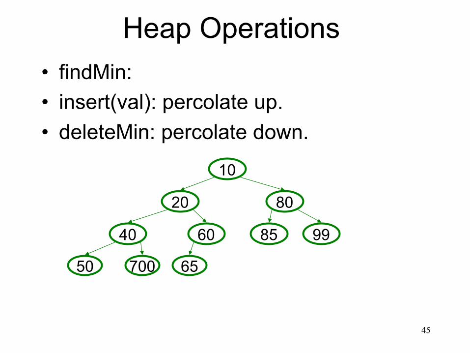
Heap Operations •  findMin: •  insert(val): percolate up. •  deleteMin: percolate down.

99 60 40

80 20

10

50 700

85

65

46

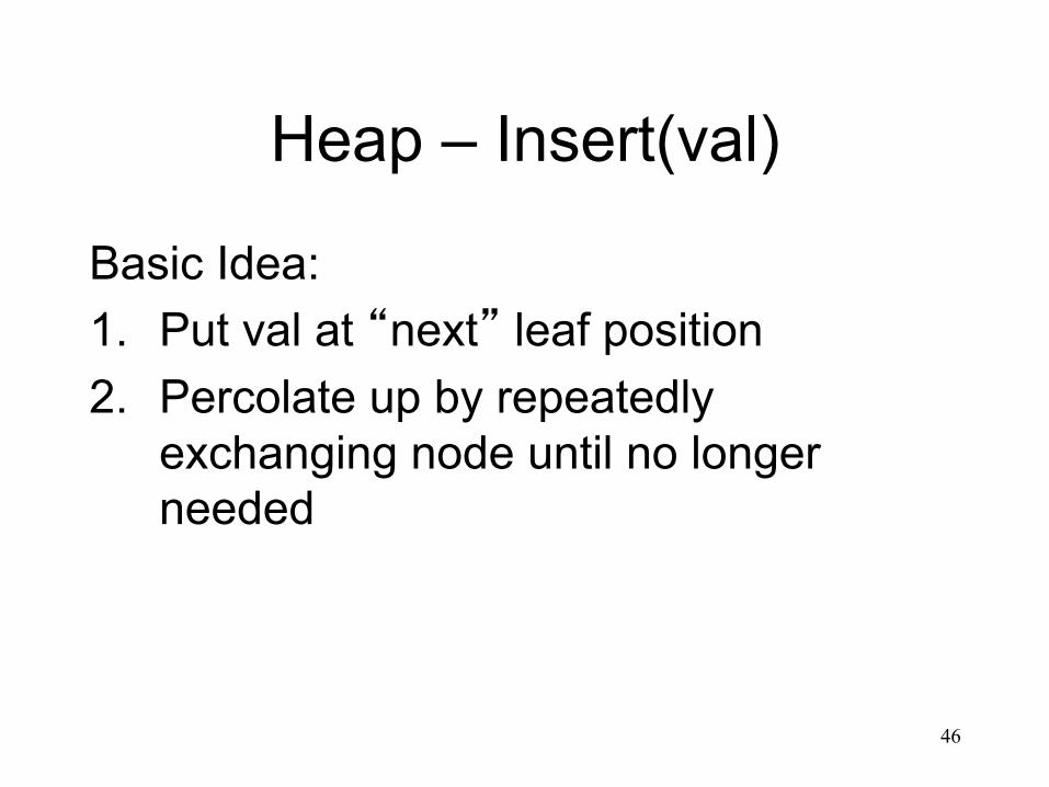
Heap – Insert(val)

Basic Idea: 1.  Put val at “next” leaf position 2.  Percolate up by repeatedly

exchanging node until no longer needed

47

Insert: percolate up

99 60 40

80 20

10

50 700

85

65 15

99 20 40

80 15

10

50 700

85

65 60

48

Insert Code (optimized) void insert(Object o) { assert(!isFull()); size++; newPos = percolateUp(size,o); Heap[newPos] = o; }

int percolateUp(int hole, Object val) { while (hole > 1 && val < Heap[hole/2]) Heap[hole] = Heap[hole/2]; hole /= 2; } return hole; }

runtime:

(Code in book)

49

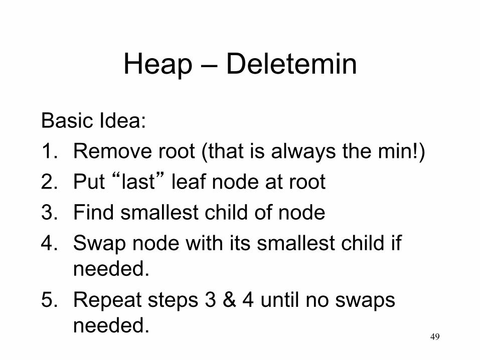
Heap – Deletemin

Basic Idea: 1.  Remove root (that is always the min!) 2.  Put “last” leaf node at root 3.  Find smallest child of node 4.  Swap node with its smallest child if

needed. 5.  Repeat steps 3 & 4 until no swaps

needed.

50

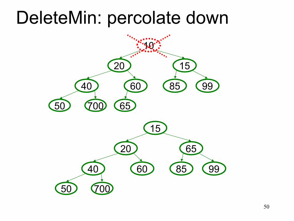
DeleteMin: percolate down

99 60 40

15 20

10

50 700

85

65

99 60 40

65 20

15

50 700

85

51

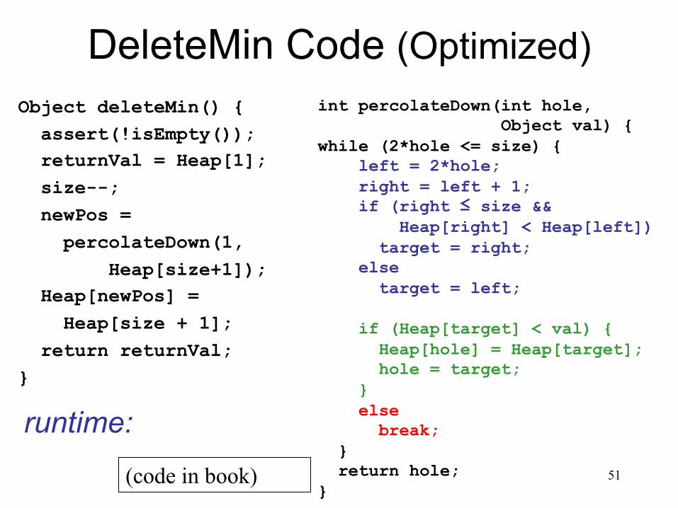
DeleteMin Code (Optimized) Object deleteMin() { assert(!isEmpty()); returnVal = Heap[1]; size--; newPos = percolateDown(1, Heap[size+1]); Heap[newPos] = Heap[size + 1]; return returnVal; }

int percolateDown(int hole, Object val) { while (2*hole <= size) { left = 2*hole; right = left + 1; if (right ≤ size && Heap[right] < Heap[left]) target = right; else target = left; if (Heap[target] < val) { Heap[hole] = Heap[target]; hole = target; } else break; } return hole; }

runtime:

(code in book)

52

0 1 2 3 4 5 6 7 8

Insert: 16, 32, 4, 69, 105, 43, 2

53

Data Structures

Binary Heaps

54

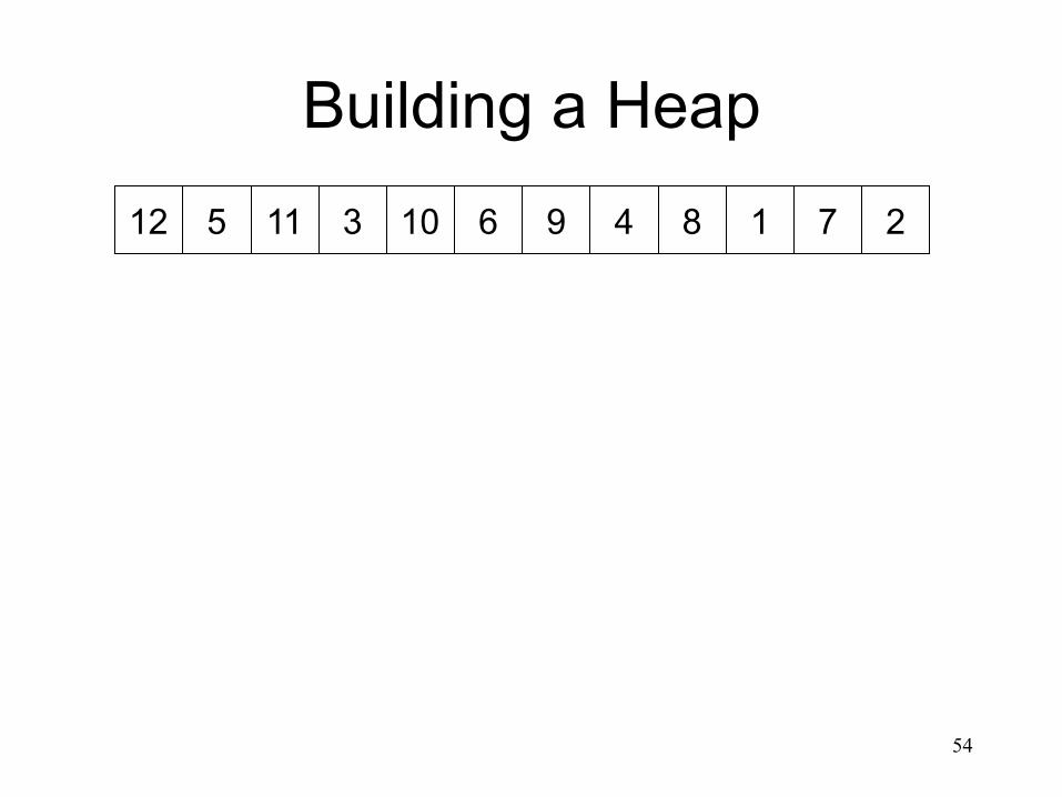
Building a Heap 5 11 3 10 6 9 4 8 1 7 2 12

55

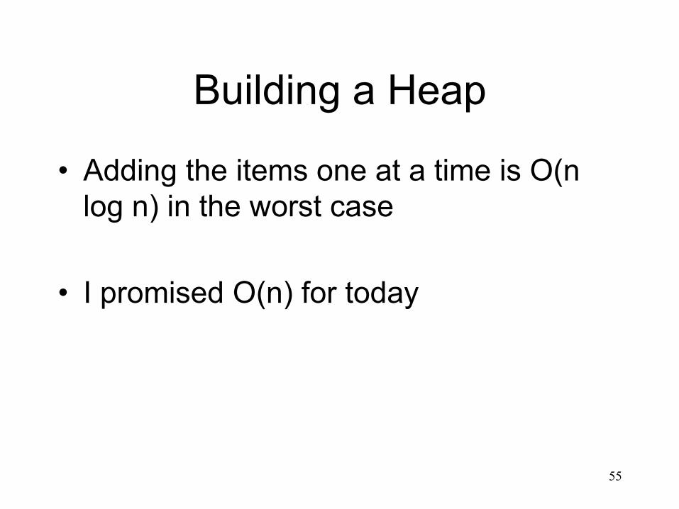
Building a Heap

•  Adding the items one at a time is O(n log n) in the worst case

•  I promised O(n) for today

56

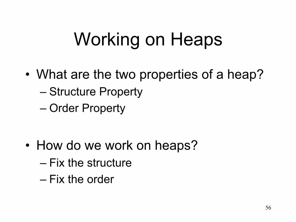
Working on Heaps

•  What are the two properties of a heap? – Structure Property – Order Property

•  How do we work on heaps? – Fix the structure – Fix the order

57

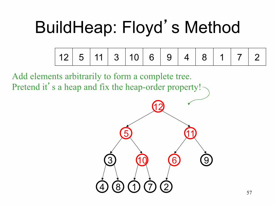
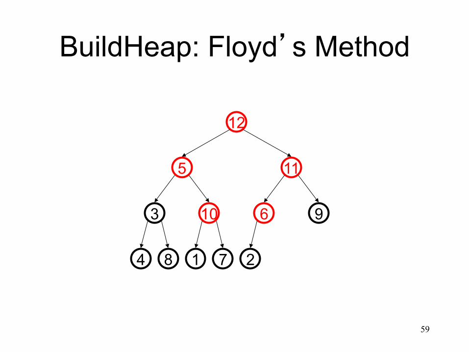
BuildHeap: Floyd’s Method 5 11 3 10 6 9 4 8 1 7 2 12

Add elements arbitrarily to form a complete tree. Pretend it’s a heap and fix the heap-order property!

2 7 1 8 4

9 6 10 3

11 5

12

58

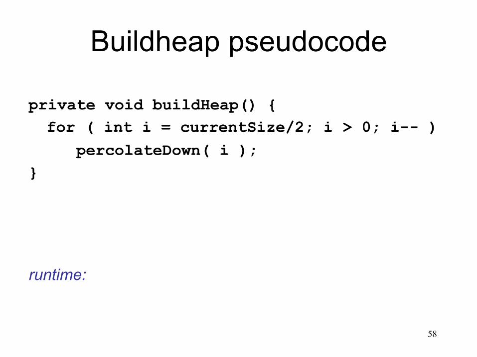
Buildheap pseudocode

private void buildHeap() { for ( int i = currentSize/2; i > 0; i-- ) percolateDown( i ); }

runtime:

59

BuildHeap: Floyd’s Method

2 7 1 8 4

9 6 10 3

11 5

12

60

BuildHeap: Floyd’s Method

6 7 1 8 4

9 2 10 3

11 5

12

61

BuildHeap: Floyd’s Method

6 7 1 8 4

9 2 10 3

11 5

12

6 7 10 8 4

9 2 1 3

11 5

12

62

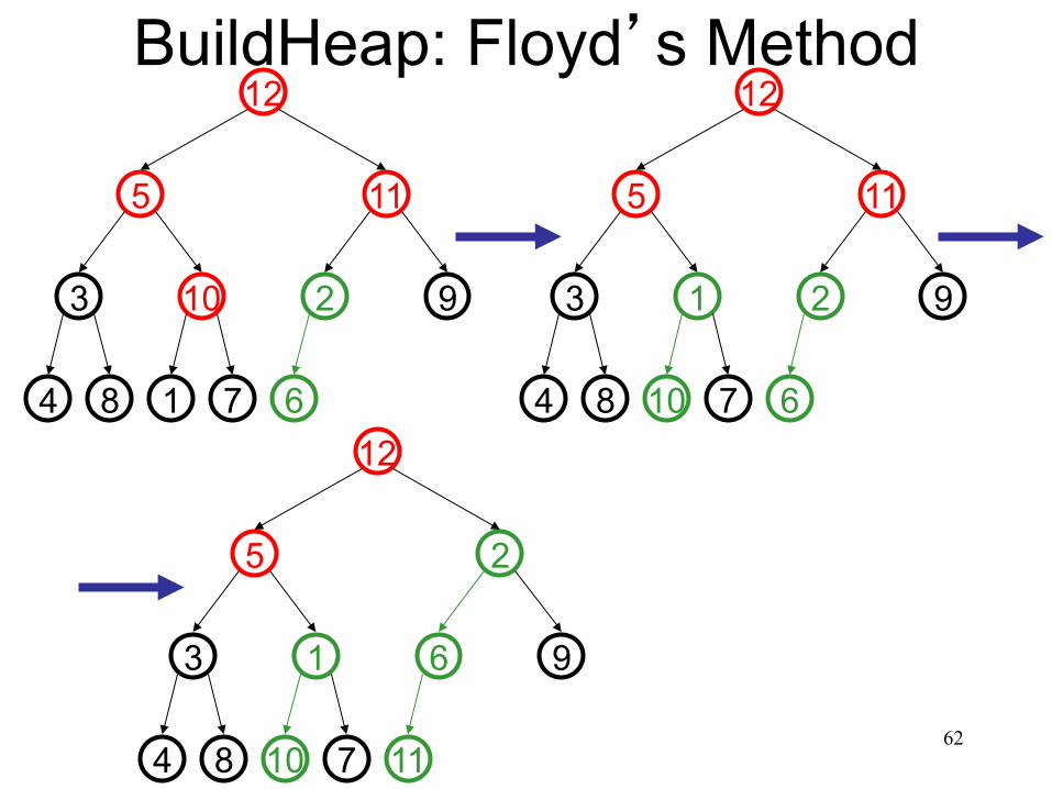
BuildHeap: Floyd’s Method

6 7 1 8 4

9 2 10 3

11 5

12

6 7 10 8 4

9 2 1 3

11 5

12

11 7 10 8 4

9 6 1 3

2 5

12

63

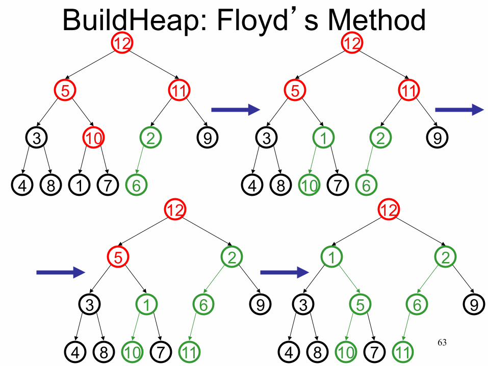
BuildHeap: Floyd’s Method

6 7 1 8 4

9 2 10 3

11 5

12

6 7 10 8 4

9 2 1 3

11 5

12

11 7 10 8 4

9 6 1 3

2 5

12

11 7 10 8 4

9 6 5 3

2 1

12

64

Finally…

11 7 10 8 12

9 6 5 4

2 3

1

runtime:

65

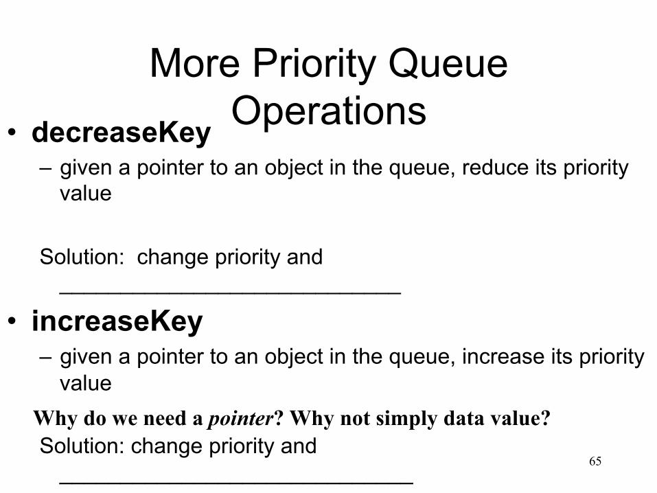
More Priority Queue Operations •  decreaseKey

–  given a pointer to an object in the queue, reduce its priority value

Solution: change priority and ____________________________

•  increaseKey –  given a pointer to an object in the queue, increase its priority

value

Solution: change priority and _____________________________

Why do we need a pointer? Why not simply data value?

66

More Priority Queue Operations •  Remove(objPtr)

– given a pointer to an object in the queue, remove the object from the queue

Solution: set priority to negative infinity, percolate up to root and deleteMin

•  FindMax

67

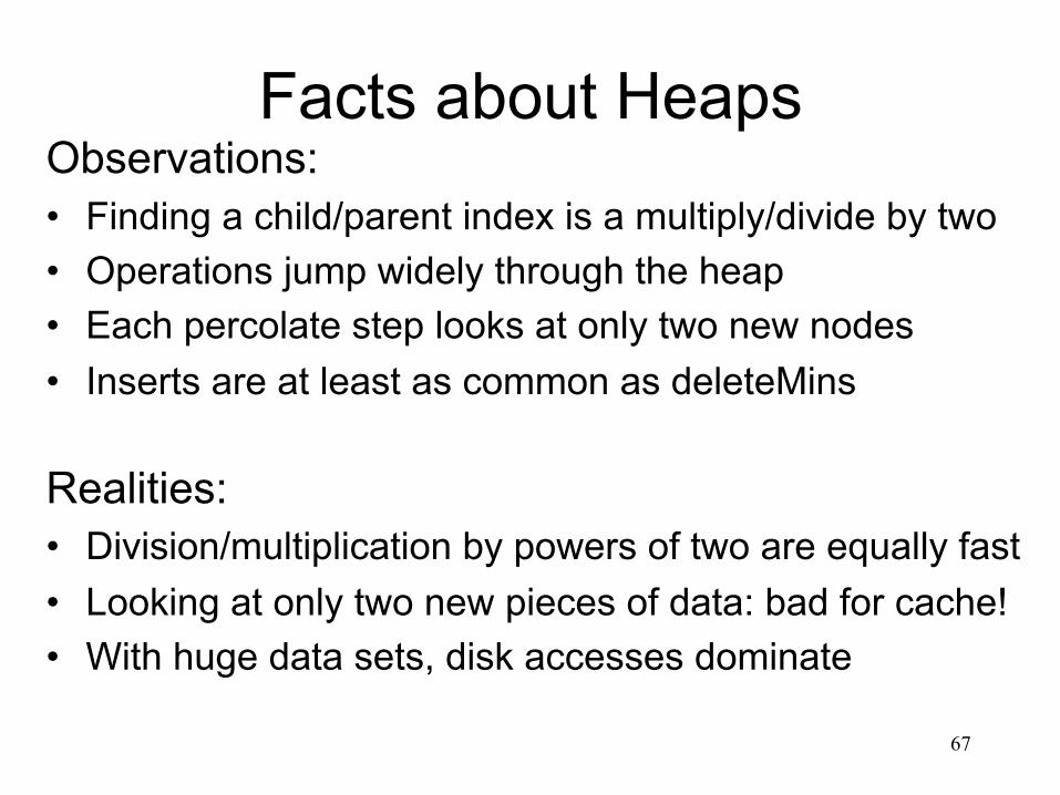
Facts about Heaps Observations: •  Finding a child/parent index is a multiply/divide by two •  Operations jump widely through the heap •  Each percolate step looks at only two new nodes •  Inserts are at least as common as deleteMins

Realities: •  Division/multiplication by powers of two are equally fast •  Looking at only two new pieces of data: bad for cache! •  With huge data sets, disk accesses dominate

68

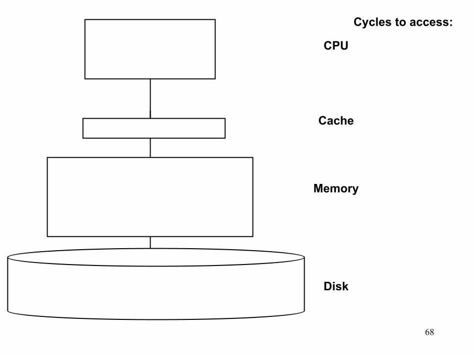
CPU

Cache

Memory

Disk

Cycles to access:

69

4

9 6 5 4

2 3

1

8 10 12

7

11

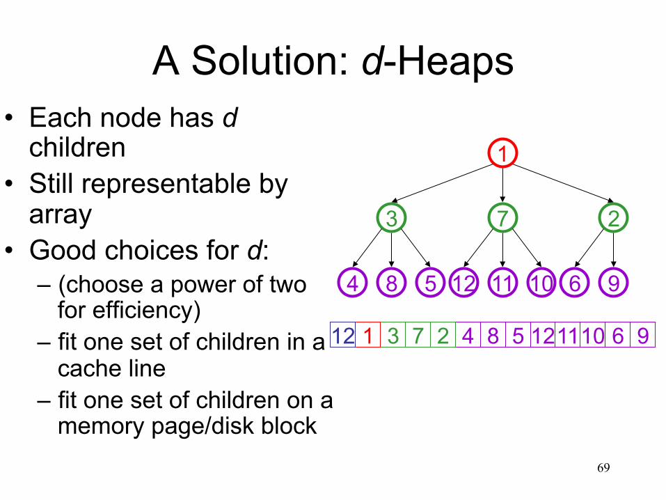
A Solution: d-Heaps •  Each node has d

children •  Still representable by

array •  Good choices for d:

–  (choose a power of two for efficiency)

–  fit one set of children in a cache line

–  fit one set of children on a memory page/disk block

3 7 2 8 5 12 11 10 6 9 1 12

Tries 70

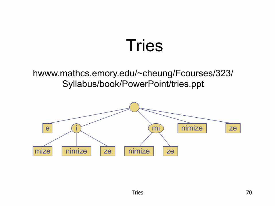
Tries

e nimize

nimize ze

zei mi

mize nimize ze

hwww.mathcs.emory.edu/~cheung/Fcourses/323/Syllabus/book/PowerPoint/tries.ppt

Tries 71

Preprocessing Strings •  Preprocessing the pattern speeds up pattern

matching queries –  After preprocessing the pattern, KMP’s algorithm performs

pattern matching in time proportional to the text size

•  If the text is large, immutable and searched for often (e.g., works by Shakespeare), we may want to preprocess the text instead of the pattern

•  A trie is a compact data structure for representing a set of strings, such as all the words in a text –  A tries supports pattern matching queries in time proportional

to the pattern size

Tries 72

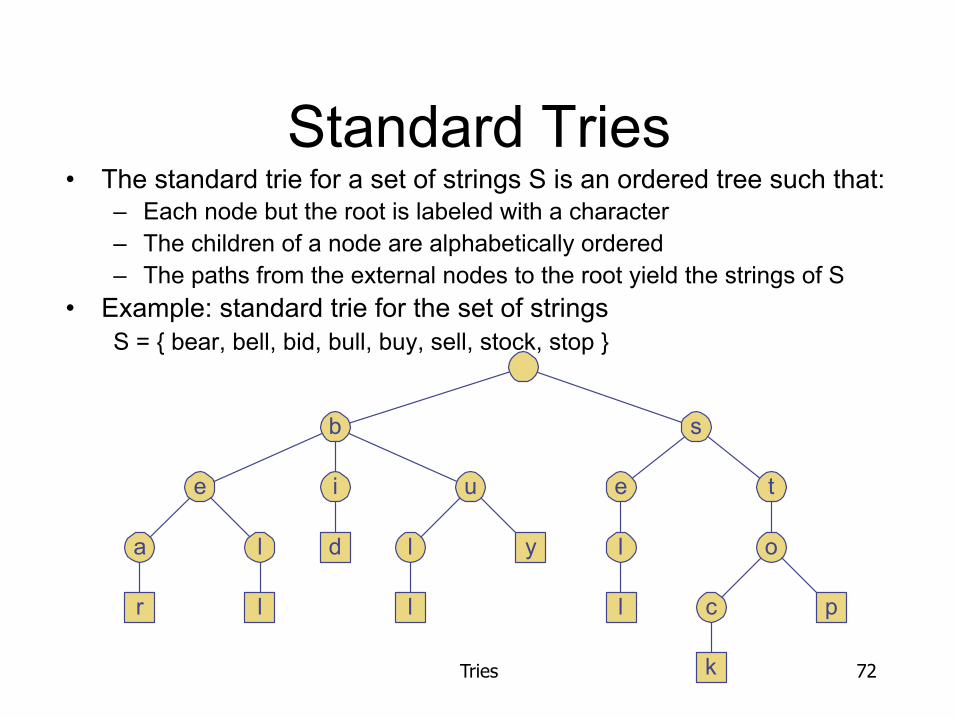
Standard Tries •  The standard trie for a set of strings S is an ordered tree such that:

–  Each node but the root is labeled with a character –  The children of a node are alphabetically ordered –  The paths from the external nodes to the root yield the strings of S

•  Example: standard trie for the set of strings S = { bear, bell, bid, bull, buy, sell, stock, stop }

a

e

b

r

l

l

s

u

l

l

y

e t

l

l

o

c

k

p

i

d

Tries 73

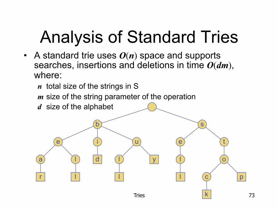
Analysis of Standard Tries •  A standard trie uses O(n) space and supports

searches, insertions and deletions in time O(dm), where: n total size of the strings in S m size of the string parameter of the operation d size of the alphabet

a

e

b

r

l

l

s

u

l

l

y

e t

l

l

o

c

k

p

i

d

Tries 74

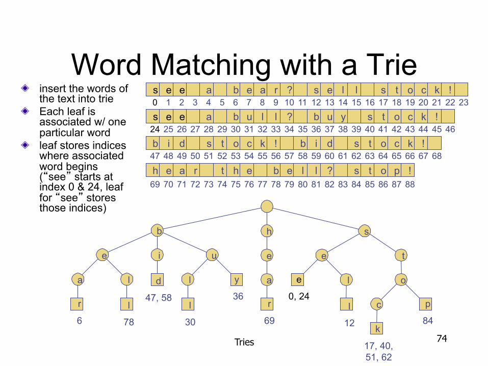
Word Matching with a Trie insert the words of the text into trie Each leaf is associated w/ one particular word leaf stores indices where associated word begins (“see” starts at index 0 & 24, leaf for “see” stores those indices)

a e

b

l

s u

l e t

e 0, 24

o c

i l

r 6

l 78

d 47, 58

l 30

y 36

l 12 k

17, 40, 51, 62

p 84

h e

r 69

a

s e e b e a r ? s e l l s t o c k ! s e e b u l l ? b u y s t o c k ! b i d s t o c k !

a a

h e t h e b e l l ? s t o p !

b i d s t o c k !

0 1 2 3 4 5 6 7 8 9 10 11 12 13 14 15 16 17 18 19 20 21 22 23 24 25 26 27 28 29 30 31 32 33 34 35 36 37 38 39 40 41 42 43 44 45 46 47 48 49 50 51 52 53 54 55 56 57 58 59 60 61 62 63 64 65 66 67 68

69 70 71 72 73 74 75 76 77 78 79 80 81 82 83 84 85 86 a r

87 88

Tries 75

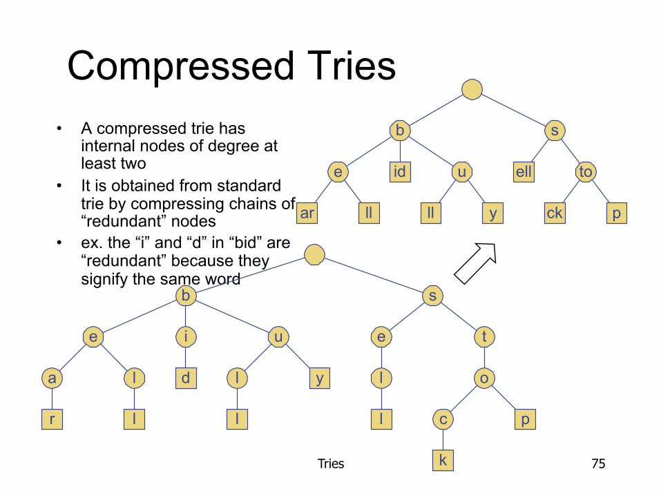
Compressed Tries •  A compressed trie has

internal nodes of degree at least two

•  It is obtained from standard trie by compressing chains of “redundant” nodes

•  ex. the “i” and “d” in “bid” are “redundant” because they signify the same word

e

b

ar ll

s

u

ll y

ell to

ck p

id

a

e

b

r

l

l

s

u

l

l

y

e t

l

l

o

c

k

p

i

d

Tries 76

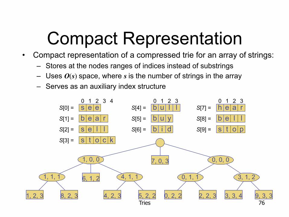
Compact Representation •  Compact representation of a compressed trie for an array of strings:

–  Stores at the nodes ranges of indices instead of substrings –  Uses O(s) space, where s is the number of strings in the array –  Serves as an auxiliary index structure

s e eb e a rs e l ls t o c k

b u l lb u yb i d

h eb e l ls t o p

0 1 2 3 4a rS[0] =

S[1] =

S[2] =

S[3] =

S[4] =

S[5] =

S[6] =

S[7] =

S[8] =

S[9] =

0 1 2 3 0 1 2 3

1, 1, 1

1, 0, 0 0, 0, 0

4, 1, 1

0, 2, 2

3, 1, 2

1, 2, 3 8, 2, 3

6, 1, 2

4, 2, 3 5, 2, 2 2, 2, 3 3, 3, 4 9, 3, 3

7, 0, 3

0, 1, 1

Tries 77

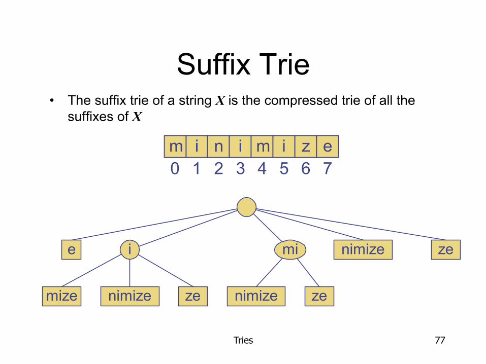
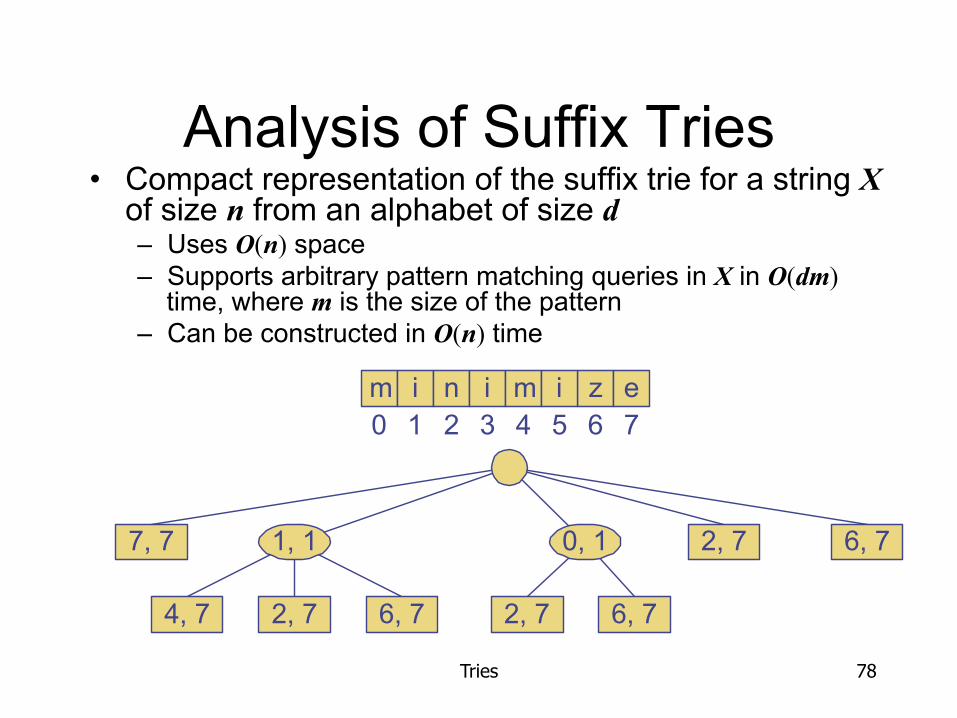
Suffix Trie •  The suffix trie of a string X is the compressed trie of all the

suffixes of X

e nimize

nimize ze

zei mi

mize nimize ze

m i n i z em i0 1 2 3 4 5 6 7

Tries 78

Analysis of Suffix Tries •  Compact representation of the suffix trie for a string X

of size n from an alphabet of size d –  Uses O(n) space –  Supports arbitrary pattern matching queries in X in O(dm)

time, where m is the size of the pattern –  Can be constructed in O(n) time

7, 7 2, 7

2, 7 6, 7

6, 7

4, 7 2, 7 6, 7

1, 1 0, 1

m i n i z em i0 1 2 3 4 5 6 7

Tries 79

Encoding Trie (1) •  A code is a mapping of each character of an alphabet to a binary

code-word •  A prefix code is a binary code such that no code-word is the prefix

of another code-word •  An encoding trie represents a prefix code

–  Each leaf stores a character –  The code word of a character is given by the path from the root to the

leaf storing the character (0 for a left child and 1 for a right child

a

b c

d e

00 010 011 10 11

a b c d e

Tries 80

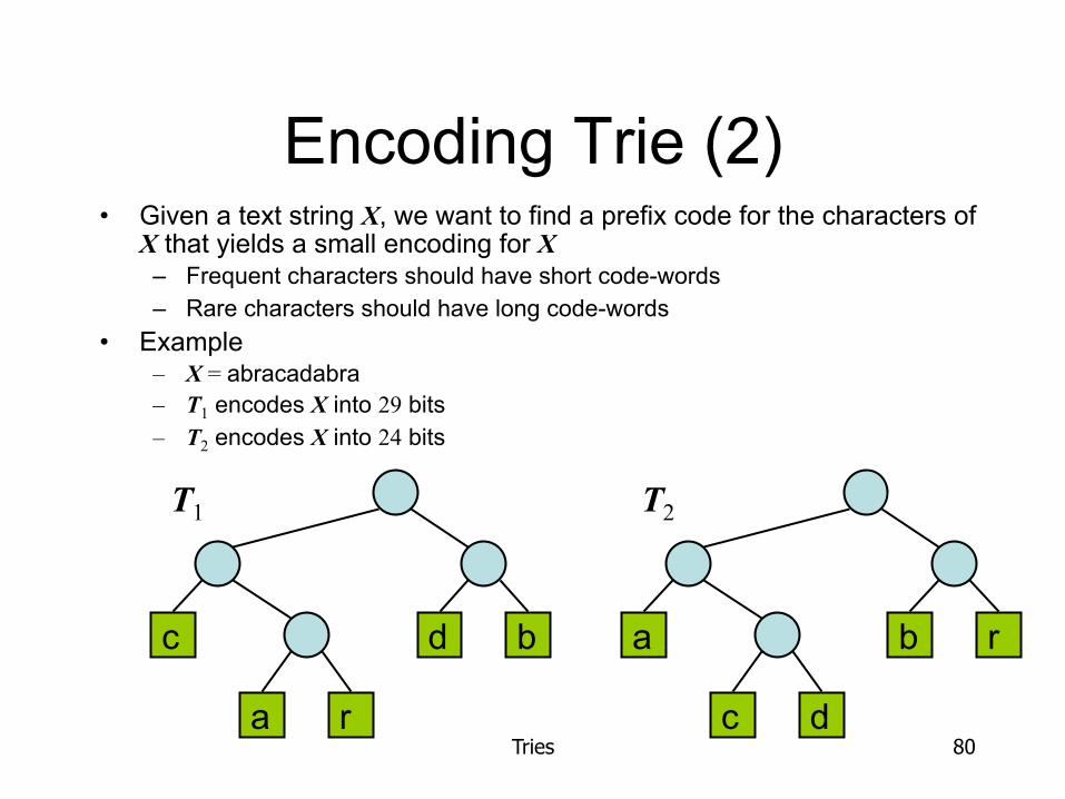
Encoding Trie (2) •  Given a text string X, we want to find a prefix code for the characters of

X that yields a small encoding for X –  Frequent characters should have short code-words –  Rare characters should have long code-words

•  Example –  X = abracadabra –  T1 encodes X into 29 bits –  T2 encodes X into 24 bits

c

a r

d b a

c d

b r

T1 T2

The End

Tries 82

Huffman’s Algorithm •  Given a string X,

Huffman’s algorithm construct a prefix code the minimizes the size of the encoding of X

•  It runs in time O(n + d log d), where n is the size of X and d is the number of distinct characters of X

•  A heap-based priority queue is used as an auxiliary structure

Algorithm HuffmanEncoding(X) Input string X of size n Output optimal encoding trie for X C ← distinctCharacters(X) computeFrequencies(C, X) Q ← new empty heap for all c ∈ C T ← new single-node tree storing c Q.insert(getFrequency(c), T) while Q.size() > 1 f1 ← Q.min() T1 ← Q.removeMin() f2 ← Q.min() T2 ← Q.removeMin() T ← join(T1, T2) Q.insert(f1 + f2, T) return Q.removeMin()

Tries 83

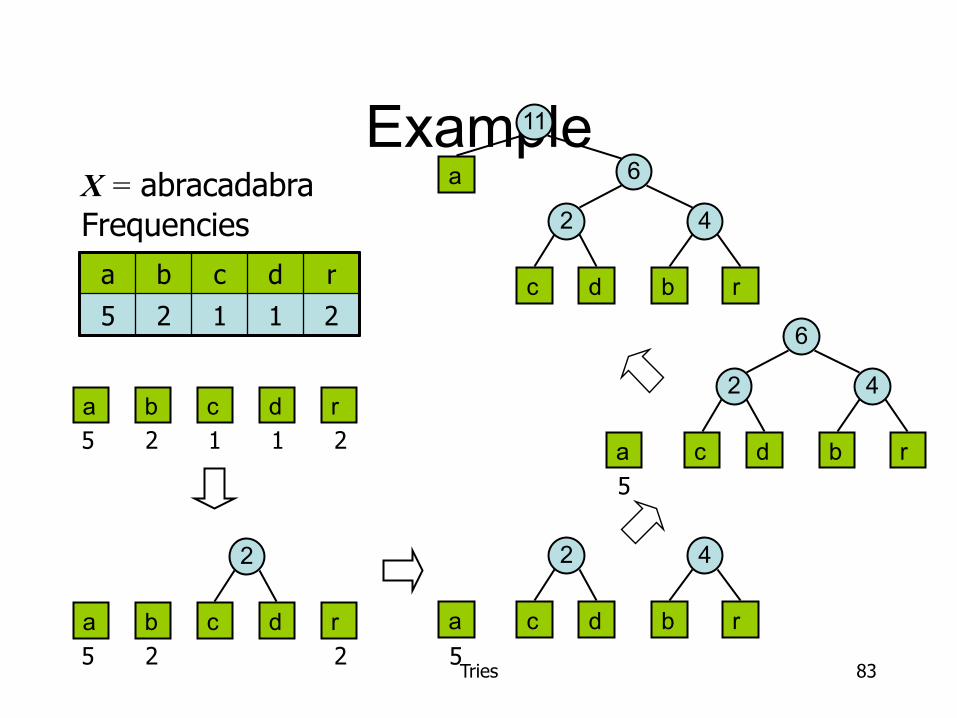
Example

a b c d r 5 2 1 1 2

X = abracadabra Frequencies

c a r d b 5 2 1 1 2

c a r d b

2

5 2 2 c a b d r

2

5

4

c a b d r

2

5

4

6

c

a

b d r

2 4

6

11

84

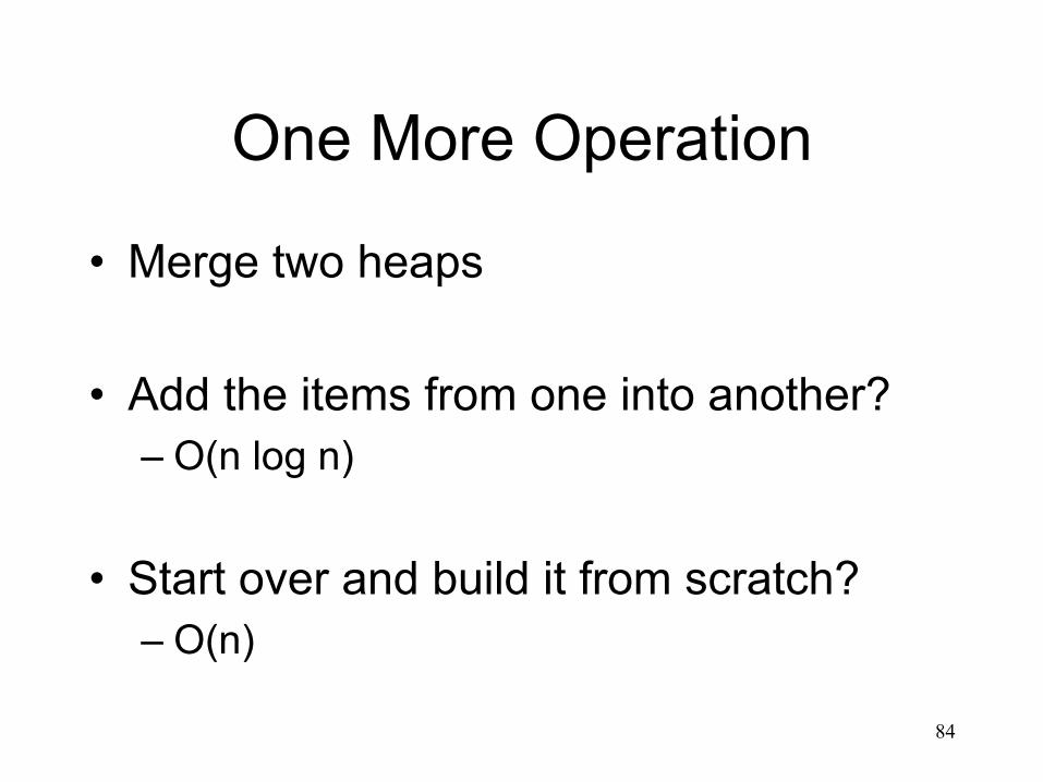
One More Operation

•  Merge two heaps

•  Add the items from one into another? – O(n log n)

•  Start over and build it from scratch? – O(n)

85

CSE 326: Data Structures

Priority Queues Leftist Heaps & Skew Heaps

86

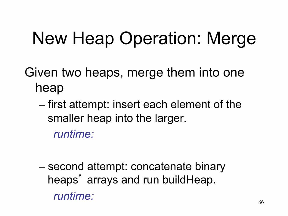
New Heap Operation: Merge

Given two heaps, merge them into one heap –  first attempt: insert each element of the

smaller heap into the larger. runtime:

– second attempt: concatenate binary heaps’ arrays and run buildHeap. runtime:

87

Leftist Heaps

Idea: Focus all heap maintenance work in one small part of the heap

Leftist heaps:

1.  Most nodes are on the left 2.  All the merging work is done on the right

88

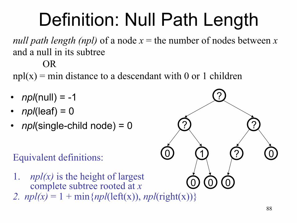
null path length (npl) of a node x = the number of nodes between x and a null in its subtree

OR npl(x) = min distance to a descendant with 0 or 1 children

Definition: Null Path Length

•  npl(null) = -1 •  npl(leaf) = 0 •  npl(single-child node) = 0

0 0 0

0 ? 1

? ?

?

Equivalent definitions: 1.  npl(x) is the height of largest

complete subtree rooted at x 2.  npl(x) = 1 + min{npl(left(x)), npl(right(x))}

0

89

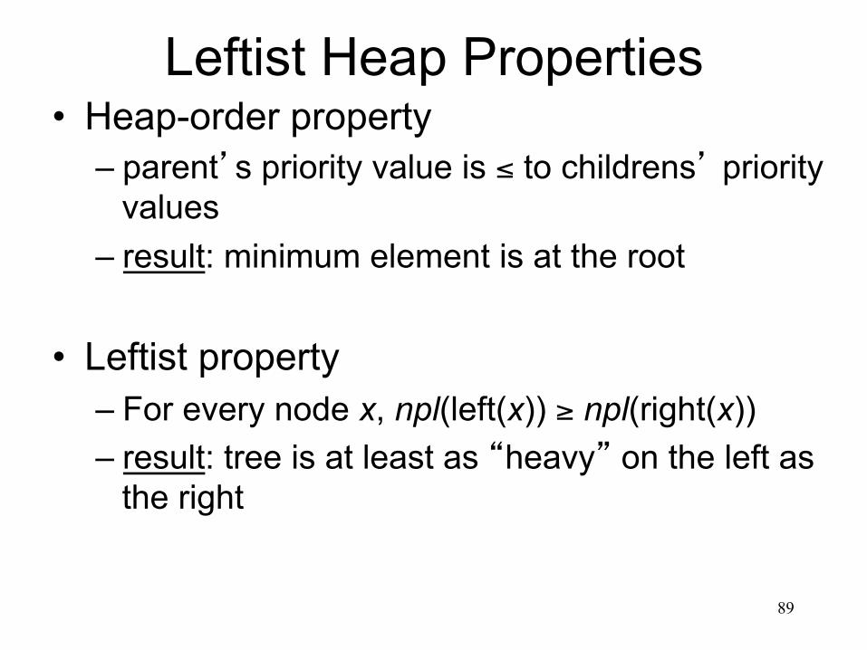
Leftist Heap Properties •  Heap-order property

– parent’s priority value is ≤ to childrens’ priority values

–  result: minimum element is at the root

•  Leftist property – For every node x, npl(left(x)) ≥ npl(right(x)) –  result: tree is at least as “heavy” on the left as

the right

90

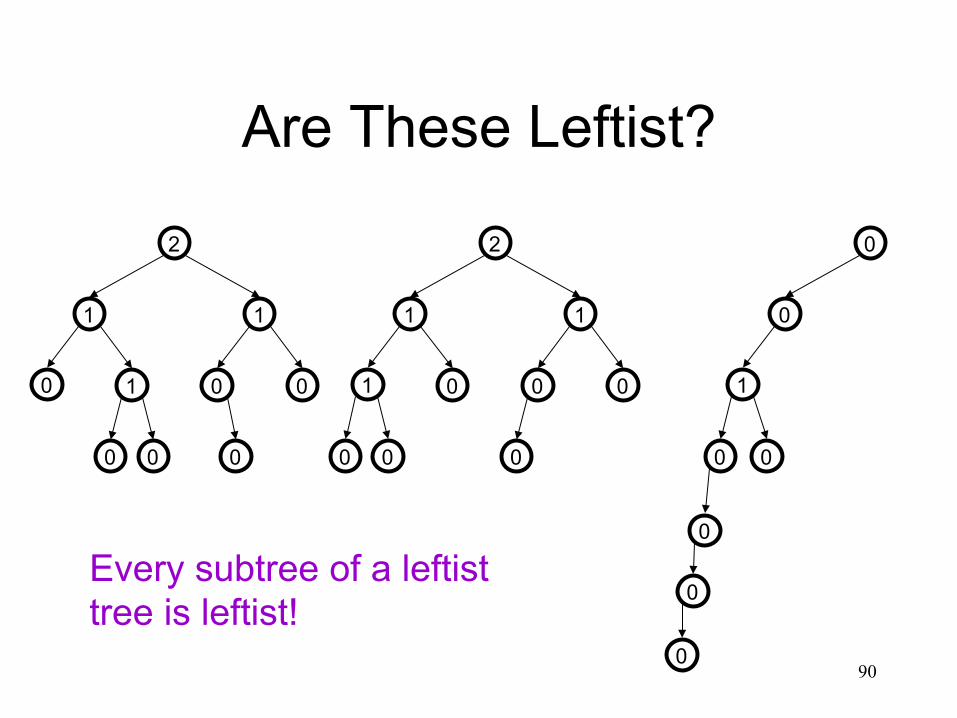
Are These Leftist?

0 0

0 0 1

1 1

2

0

0

0 0 0

1 1

2

1

0 0 0

0

0

0

0

0

1

0 0

Every subtree of a leftist tree is leftist!

91

Right Path in a Leftist Tree is Short (#1) Claim: The right path is as short as any in the

tree. Proof: (By contradiction)

R

x

L D2

D1

Pick a shorter path: D1 < D2 Say it diverges from right path at x npl(L) ≤ D1-1 because of the path of length D1-1 to null npl(R) ≥ D2-1 because every node on right path is leftist

Leftist property at x violated!

92

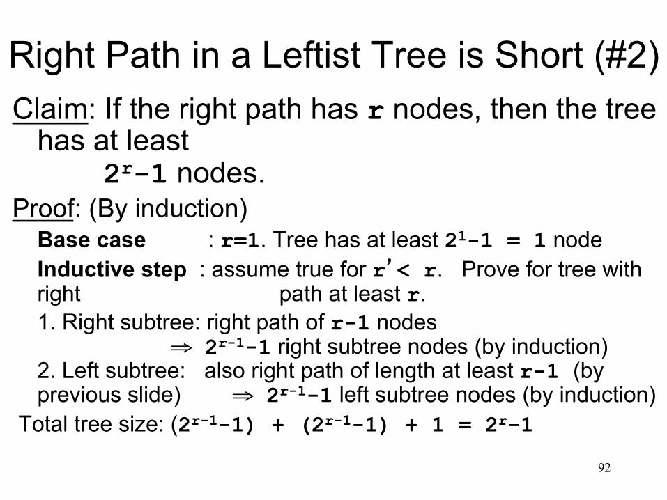
Right Path in a Leftist Tree is Short (#2) Claim: If the right path has r nodes, then the tree

has at least 2r-1 nodes.

Proof: (By induction)

Base case : r=1. Tree has at least 21-1 = 1 node Inductive step : assume true for r’< r. Prove for tree with right path at least r. 1. Right subtree: right path of r-1 nodes

⇒ 2r-1-1 right subtree nodes (by induction) 2. Left subtree: also right path of length at least r-1 (by previous slide) ⇒ 2r-1-1 left subtree nodes (by induction)

Total tree size: (2r-1-1) + (2r-1-1) + 1 = 2r-1

93

Why do we have the leftist property?

Because it guarantees that: •  the right path is really short compared to

the number of nodes in the tree •  A leftist tree of N nodes, has a right path

of at most lg (N+1) nodes

Idea – perform all work on the right path

94

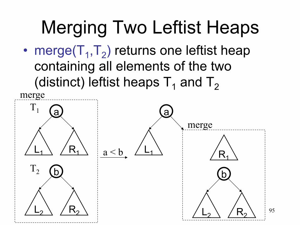
Merge two heaps (basic idea)

•  Put the smaller root as the new root, •  Hang its left subtree on the left. •  Recursively merge its right subtree and

the other tree.

95

Merging Two Leftist Heaps •  merge(T1,T2) returns one leftist heap

containing all elements of the two (distinct) leftist heaps T1 and T2

a

L1 R1

b

L2 R2

merge T1

T2 a < b

a

L1

merge

b

L2 R2

R1

96

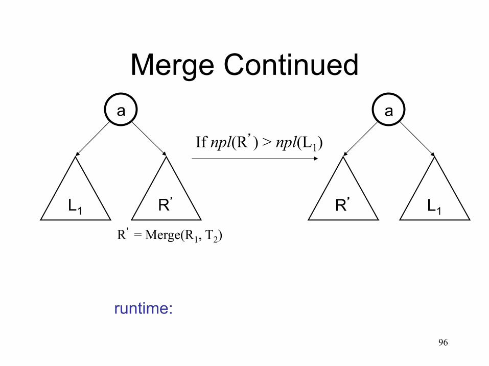
Merge Continued a

L1 R’

R’ = Merge(R1, T2)

a

R’ L1

If npl(R’) > npl(L1)

runtime:

97

Let’s do an example, but first… Other Heap Operations

•  insert ?

•  deleteMin ?

98

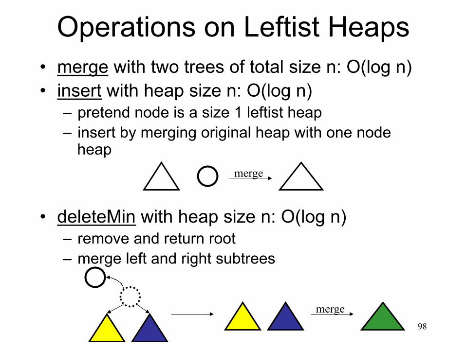
Operations on Leftist Heaps •  merge with two trees of total size n: O(log n) •  insert with heap size n: O(log n)

–  pretend node is a size 1 leftist heap –  insert by merging original heap with one node

heap

•  deleteMin with heap size n: O(log n)

–  remove and return root –  merge left and right subtrees

merge

merge

99

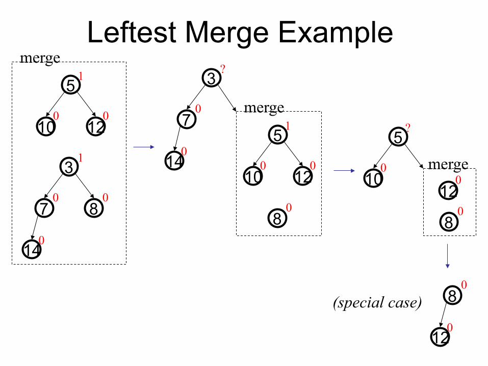
Leftest Merge Example

12 10

5

8 7

3

14

1

0 0

1

0 0

0

merge

7

3

14

?

0

0

12 10

5

8

1

0 0

0

merge

10

5 ?

0 merge

12

8

0

0

8

12

0

0

(special case)

100

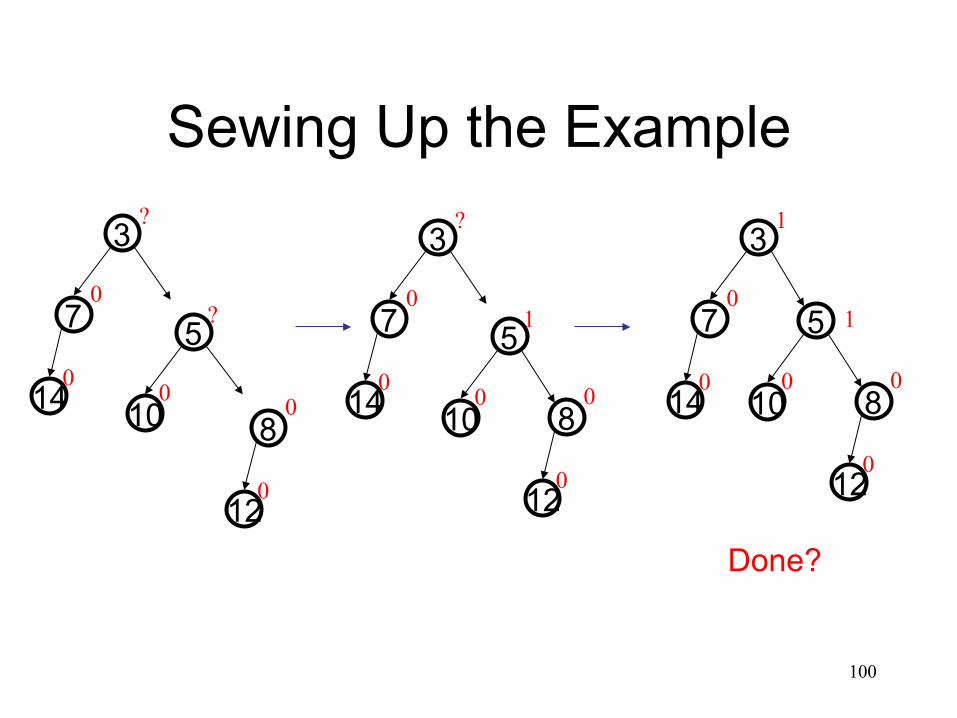
Sewing Up the Example

8

12

0

0

10

5 ?

0

7

3

14

?

0

0

8

12

0

0

10

5 1

0

7

3

14

?

0

0 8

12

0

0

10

5 1

0

7

3

14

1

0

0

Done?

101

Finally…

8

12

0

0

10

5 1

0

7

3

14

1

0

0

7

3

14

1

0

0 8

12

0

0

10

5 1

0

102

Leftist Heaps: Summary

Good •  • 

Bad •  • 

103

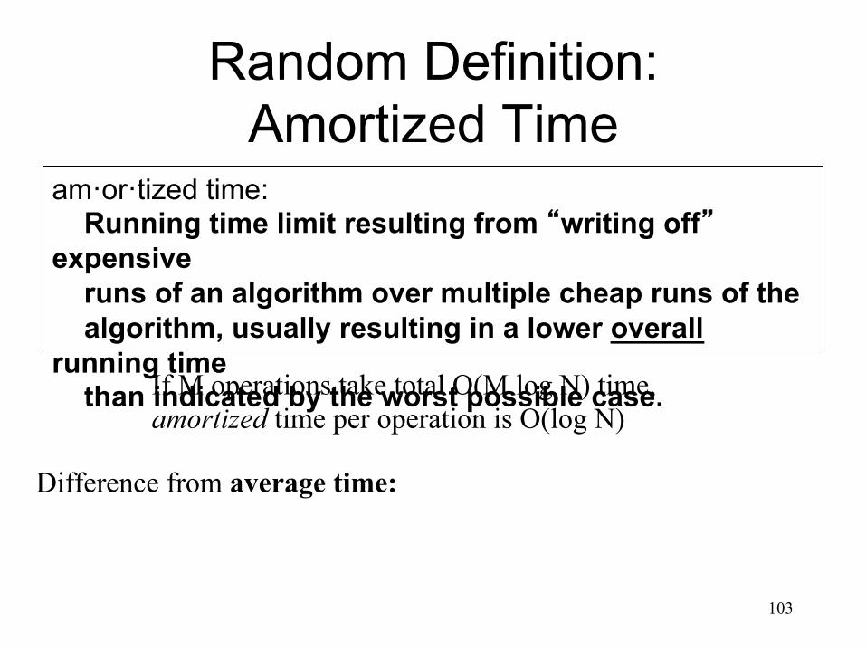
Random Definition: Amortized Time

am·or·tized time: Running time limit resulting from “writing off” expensive runs of an algorithm over multiple cheap runs of the algorithm, usually resulting in a lower overall running time than indicated by the worst possible case. If M operations take total O(M log N) time,

amortized time per operation is O(log N)

Difference from average time:

104

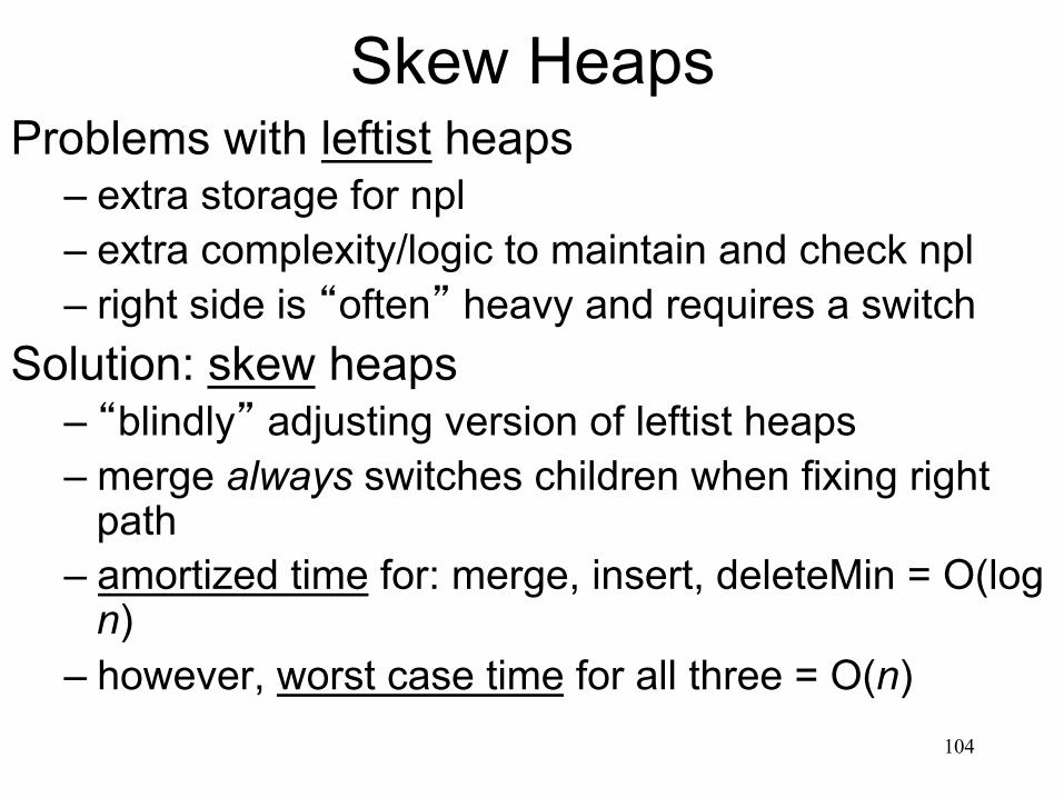
Skew Heaps Problems with leftist heaps

– extra storage for npl – extra complexity/logic to maintain and check npl –  right side is “often” heavy and requires a switch

Solution: skew heaps – “blindly” adjusting version of leftist heaps – merge always switches children when fixing right

path – amortized time for: merge, insert, deleteMin = O(log

n) – however, worst case time for all three = O(n)

105

Merging Two Skew Heaps

a

L1 R1

b

L2 R2

merge T1

T2

a < b

a

L1

merge

b

L2 R2

R1

Only one step per iteration, with children always switched

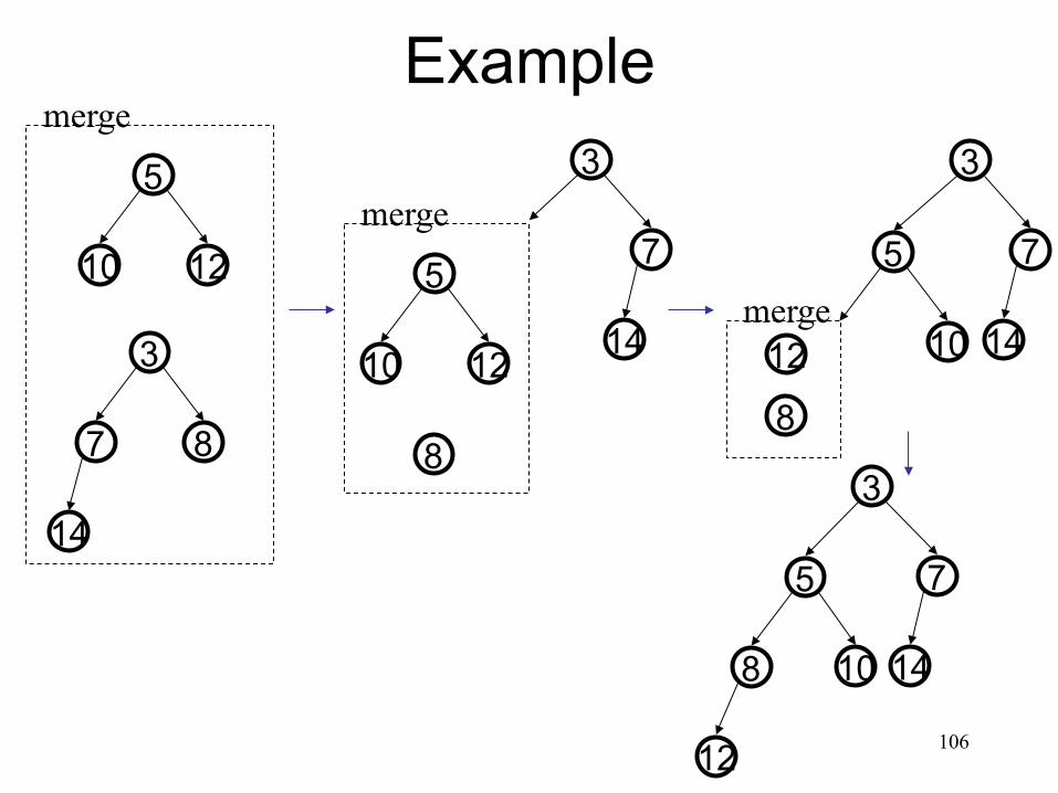
106

Example

12 10

5

8 7

3

14

merge

7

3

14 12 10

5

8

merge 7

3

14 10

5

8

merge 12

7

3

14 10 8

5

12

107

Skew Heap Code void merge(heap1, heap2) { case { heap1 == NULL: return heap2; heap2 == NULL: return heap1; heap1.findMin() < heap2.findMin(): temp = heap1.right; heap1.right = heap1.left; heap1.left = merge(heap2, temp); return heap1; otherwise: return merge(heap2, heap1); } }

108

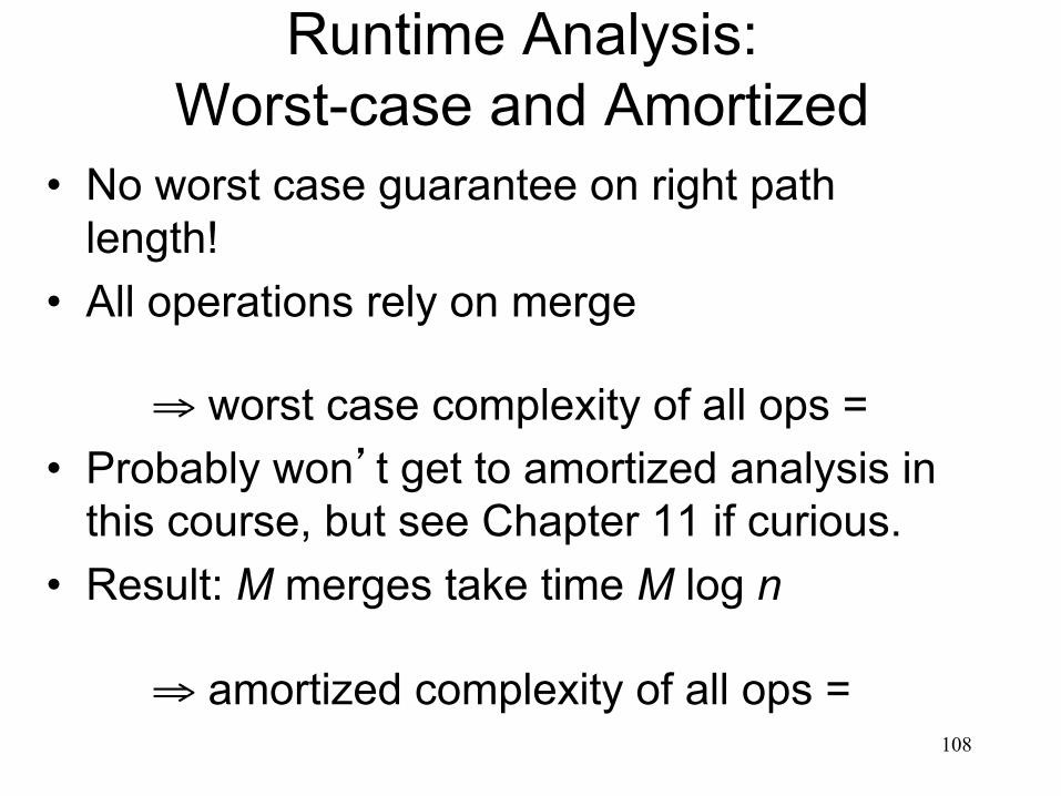
Runtime Analysis: Worst-case and Amortized

•  No worst case guarantee on right path length!

•  All operations rely on merge

⇒ worst case complexity of all ops = •  Probably won’t get to amortized analysis in

this course, but see Chapter 11 if curious. •  Result: M merges take time M log n

⇒ amortized complexity of all ops =

109

Comparing Heaps •  Binary Heaps

•  d-Heaps

•  Leftist Heaps

•  Skew Heaps

Still room for improvement! (Where?)

Data Structures Binomial Queues

110

Yet Another Data Structure: Binomial Queues

•  Structural property – Forest of binomial trees with at most

one tree of any height

•  Order property – Each binomial tree has the heap-order

property

111

What’s a forest? What’s a binomial tree?

The Binomial Tree, Bh •  Bh has height h and exactly 2h nodes •  Bh is formed by making Bh-1 a child of another Bh-1 •  Root has exactly h children •  Number of nodes at depth d is binomial coeff.

–  Hence the name; we will not use this last property

⎟⎟⎠

⎞⎜⎜⎝

⎛

dh

112

B0 B1 B2 B3

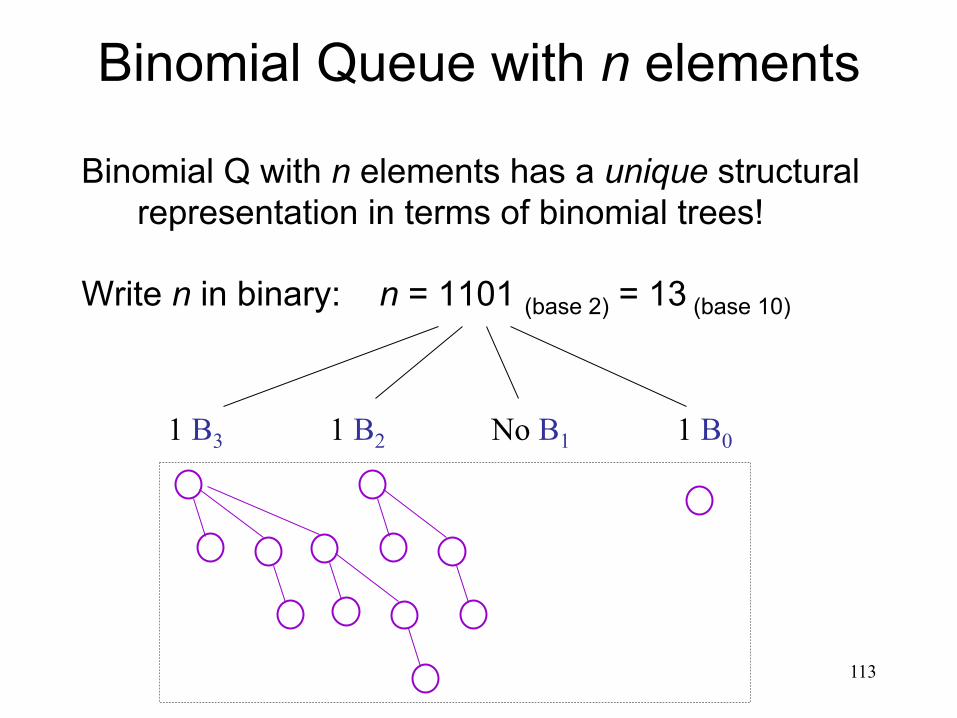
Binomial Queue with n elements

Binomial Q with n elements has a unique structural representation in terms of binomial trees!

Write n in binary: n = 1101 (base 2) = 13 (base 10)

113

1 B3 1 B2 No B1 1 B0

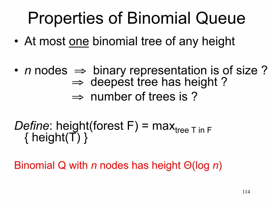
Properties of Binomial Queue •  At most one binomial tree of any height

•  n nodes ⇒ binary representation is of size ? ⇒ deepest tree has height ?

⇒ number of trees is ?

Define: height(forest F) = maxtree T in F { height(T) }

Binomial Q with n nodes has height Θ(log n)

114

Operations on Binomial Queue

•  Will again define merge as the base operation –  insert, deleteMin, buildBinomialQ will use merge

•  Can we do increaseKey efficiently? decreaseKey?

•  What about findMin?

115

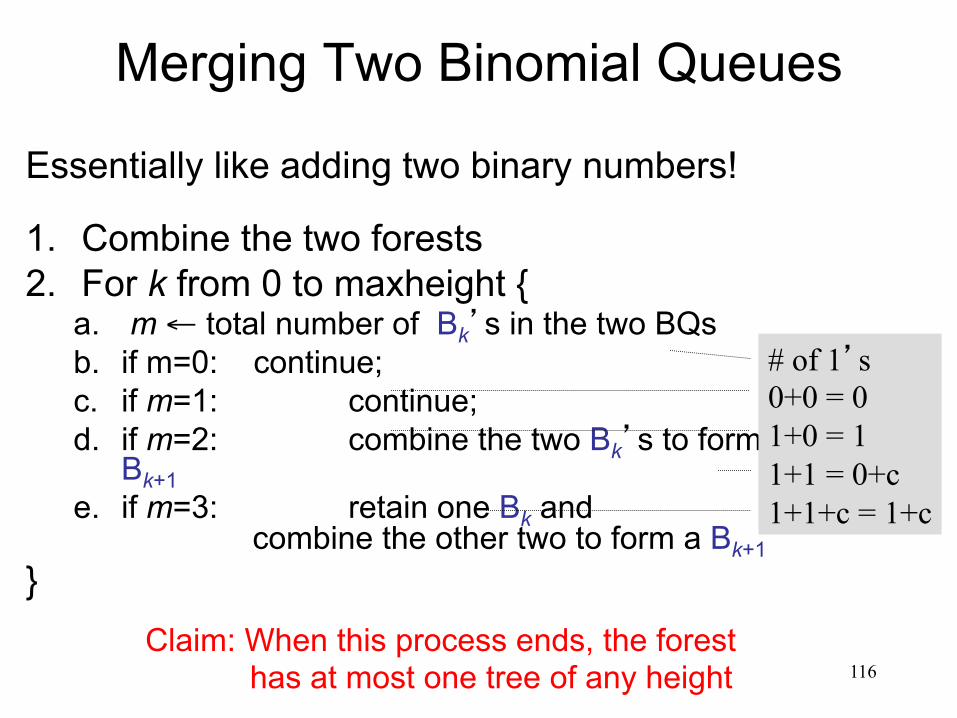
Merging Two Binomial Queues

Essentially like adding two binary numbers!

1.  Combine the two forests 2.  For k from 0 to maxheight {

a.  m ← total number of Bk’s in the two BQs b.  if m=0: continue; c.  if m=1: continue; d.  if m=2: combine the two Bk’s to form a

Bk+1 e.  if m=3: retain one Bk and

combine the other two to form a Bk+1 }

116 Claim: When this process ends, the forest

has at most one tree of any height

# of 1’s 0+0 = 0 1+0 = 1 1+1 = 0+c 1+1+c = 1+c

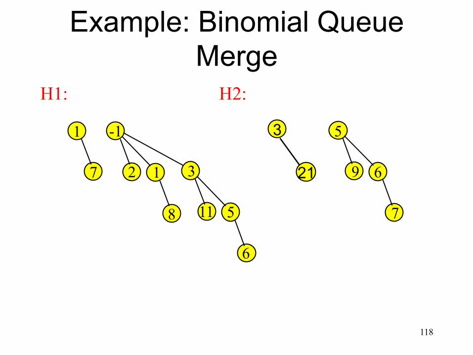
Example: Binomial Queue Merge

117

3 1

7

-1

2 1 3

8 11 5

6

5

9 6

7

21

H1: H2:

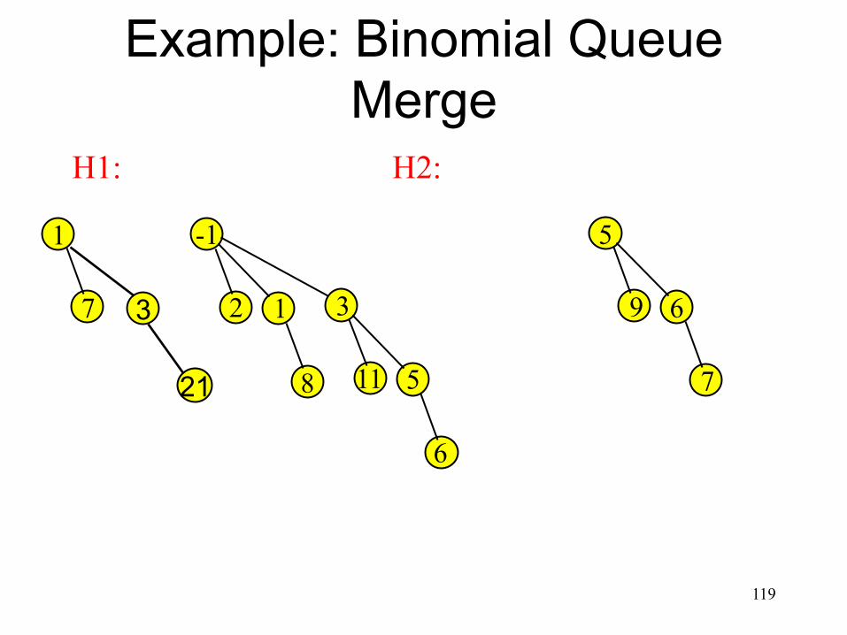
Example: Binomial Queue Merge

118

3 1

7

-1

2 1 3

8 11 5

6

5

9 6

7

21

H1: H2:

Example: Binomial Queue Merge

119

3

1

7

-1

2 1 3

8 11 5

6

5

9 6

7 21

H1: H2:

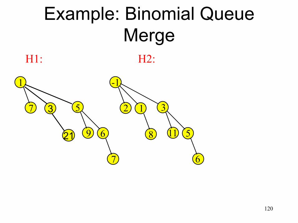
Example: Binomial Queue Merge

120

3

1

7

-1

2 1 3

8 11 5

6

5

9 6

7

21

H1: H2:

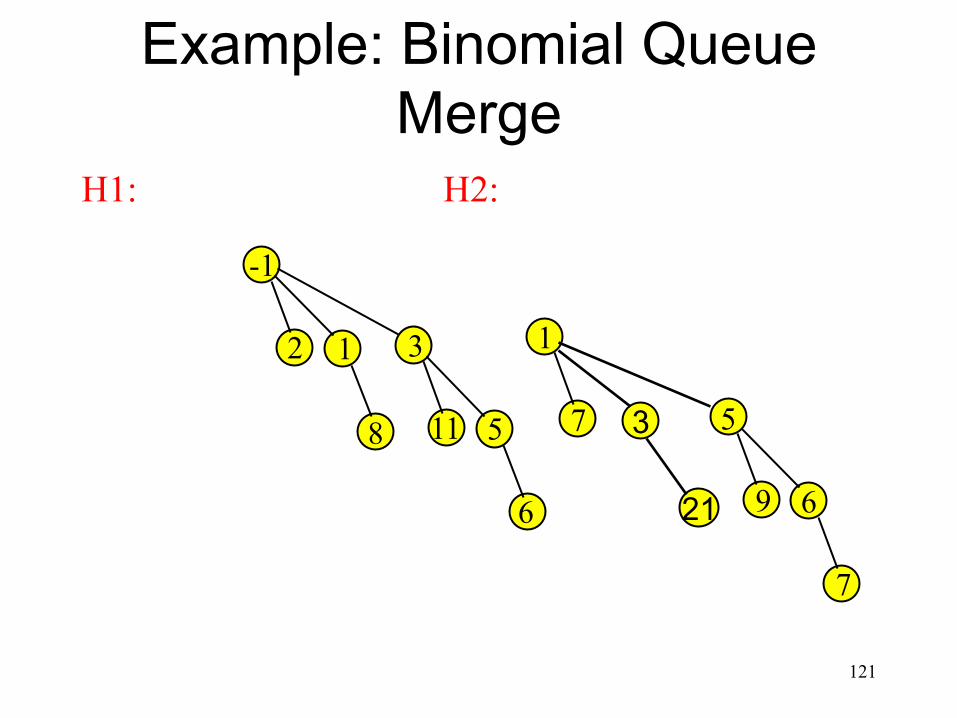
Example: Binomial Queue Merge

121

3

1

7

-1

2 1 3

8 11 5

6

5

9 6

7

21

H1: H2:

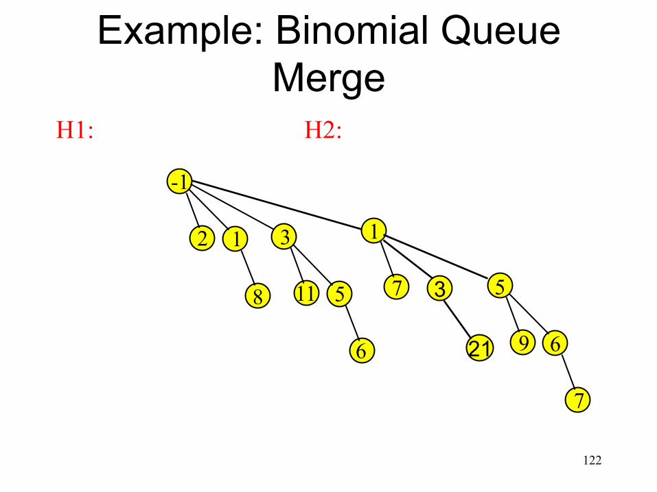
Example: Binomial Queue Merge

122

3

1

7

-1

2 1 3

8 11 5

6

5

9 6

7

21

H1: H2:

Complexity of Merge

Constant time for each height Max number of heights is: log n

⇒ worst case running time = Θ( )

123

Insert in a Binomial Queue Insert(x): Similar to leftist or skew heap

runtime Worst case complexity: same as merge O( )

Average case complexity: O(1) Why?? Hint: Think of adding 1 to 1101

124

deleteMin in Binomial Queue Similar to leftist and skew heaps….

125

deleteMin: Example

126

4 8

3

7

5

7 BQ

8

7

5

find and delete smallest root merge BQ

(without the shaded part) and BQ’

BQ’

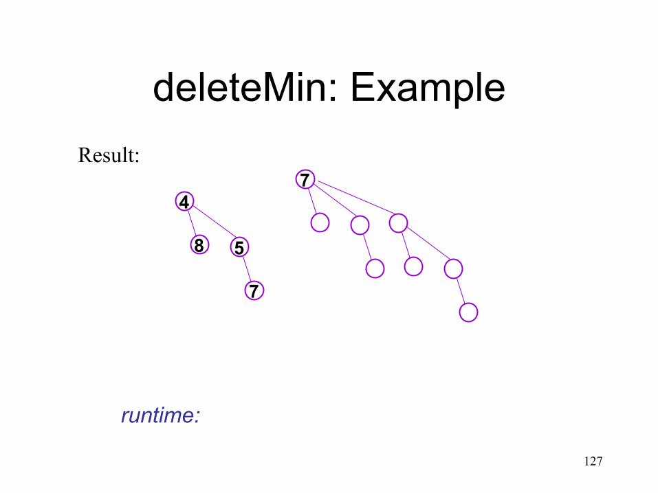
deleteMin: Example

127

8

4

7

5

7 Result:

runtime: