• NCEP =National Centers for Environmental Prediction

• Weather Research and Forecasting Non-hydrostatic Mesoscale Model (WRF-NMM)** model is run as the NAM – three names (NAM, WRF, or NMM) refer to the same model output

• run at 00,06,12,18Z and forecasting to 84 hours

• domain is regional, horizontal resolution =12 km, outputs every hour

• dynamics: fully compressible, non-hydrostatic (with hydrostatic option)

• one-way or two-way nesting

• staggered grid

**Distinct from WRF-ARW, which has the ARW "dynamical core". NMM core is much faster than ARW

eas372_NWP_NCEP_2017.odpJDW, EAS, U. AlbertaLast modified 4 Apr., 2017

www.wrf-model.org/index.phpwww2.mmm.ucar.edu/wrf/users/www.dtcenter.org/wrf-nmm/users/en.wikipedia.org/wiki/North_American_Mesoscale_Model

NCEP’s "NAM" (North American Mesoscale) model WRF-NMM

• Cartesian velocity components u,v,w; perturbations of potential temperature , geopotential Φ (=g Z), and surface pressure of dry air from their values in a hydrostatic referencestate; also turbulent kinetic energy k , water vapor mixing ratio r, rain/snow mixing ratio, and cloud water/ice mixing ratio

• vertical coord (60 levels)

where is the hydrostatic component of the pressure, computed using the dry air density

and S and T its values along the surface and top boundaries (Laprise, 1992; MWR Vol. 120). If zT is placed at infinity then T=0 and is simply the hydrostatic partial pressure of the dry air.

• is a terrain-following coordinate

η=−TS−T

( x , y , z , t )=T+∫z

zT

ρd ( x , y , z ', t ) g dz '

NCEP’s "NAM" (North American Mesoscale) model WRF-NMM

NAM's parameterizations

• eddy viscosity/diffusivity K based on turbulent kinetic energy equation

Vertical transport by unresolved scales of motion

Radiation

• clear-sky absorbers: dynamic** water vapour; uniformly mixed (330 ppm) CO2; latitudinally and seasonally varying climatological ozone; solar constant chopped by 3% to account for aerosols

• solar computations hourly; two streams diffuse & one (downward) stream direct; spectrum divided into two bands each carrying apprx. 50% of the energy: UV/visible and near infrared

• longwave computations hourly , >100 bands **meaning, interacts with model's resolved humidity field

Clouds and precip

• Betts-Miller-Janjic deep convection, column moist adjustment towards a well-mixed profile (moist adiabatic)

• convective precip (falls instantly) determined as change of precipitable water as model sounding forced to moist adiabat between LFC and LNB; tracks liquid cloud drops, raindrops, small & lrg ice particles

Coupling to surface

• 4 layer soil with vegetation. Remote sensing data for vegetation type and “greenness fraction”

• daily remotely sensed observations to update snow cover and water equivalent snow depth. A snow density variable is used, and the predicted percentage of frozen precipitation reaching the surface updates the snow budget

• water surfaces held at initially observed temperature. Each grid box is designated as having a land or water surface - but no subgrid structure

• let w=W+w’, q=Q+q’ where w, q are the (total) vertical velocity and humidity, W, Q are resolved vertical velocity and humidity, and the primes represent the sub-grid (hidden, fluctuating) motion. Then the total vertical humidity flux

where W Q is the resolved flux, remainder the subgrid flux

• a second-order closure scheme invokes simplified budget equations for the subgrid fluxes themselves (these may be derived from the Navier-Stokes equations and the thermodynamic and humidity conservation eqns), e.g.

w q = W Q + w ' q'

(note: used in research, but not, so far, in NWP)

flux advection

flux production flux decay

flux diffusion

local tendency in time

effectively a diffusivity

[ ∂∂ t+U ∂

∂ x+ V ∂

∂ y+ W ∂

∂ z ] w ' q '=− w '2 ∂Q∂ z

+ ∂∂ z [w '2 τ ∂w ' q '

∂ z ] − w ' q 'τ

Advanced models (“higher-order closures”) for transport by unresolved scales of motion

+ g0

ρ0 q ' '

variance of the unresolved vertical velocity… the mean-square value of the fluctuation w’ . It is equal, by definition, to the square of the standard deviation of w’, ie.

w' 2

w '2≡σw2

and it cannot be negative.

z

Q

Gradient in resolved humidity in conjunction with fluctuating vertical motion… producing vertical humidity transport. In this case, one intuitively expects a positive, ie. an upward, flux. However although the flux production term is (in the case shown at the left) positive, the budget equation does not mandate that the flux should run down the “driving” gradient. This treatment allows “counter-gradient” fluxes, which indeed are observed at some times in some places

is the “timescale” of the unresolved vertical velocity

Effective (vertical) diffusivity attributed to unresolved motion

τ = λσw

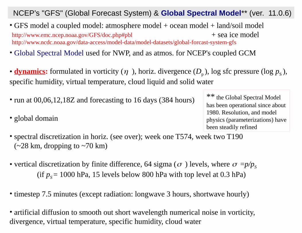
NCEP’s "GFS" (Global Forecast System) & Global Spectral Model** (ver. 11.0.6)

• GFS model a coupled model: atmosphere model + ocean model + land/soil model + sea ice model

• Global Spectral Model used for NWP, and as atmos. for NCEP's coupled GCM

• dynamics: formulated in vorticity ( ), horiz. divergence (Dp ), log sfc pressure (log pS ), specific humidity, virtual temperature, cloud liquid and solid water

• run at 00,06,12,18Z and forecasting to 16 days (384 hours)

• global domain

• spectral discretization in horiz. (see over); week one T574, week two T190 (~28 km, dropping to ~70 km)

• vertical discretization by finite difference, 64 sigma (σ ) levels, where σ =p/pS (if pS = 1000 hPa, 15 levels below 800 hPa with top level at 0.3 hPa)

• timestep 7.5 minutes (except radiation: longwave 3 hours, shortwave hourly)

• artificial diffusion to smooth out short wavelength numerical noise in vorticity, divergence, virtual temperature, specific humidity, cloud water

** the Global Spectral Model has been operational since about 1980. Resolution, and model physics (parameterizations) have been steadily refined

http://www.emc.ncep.noaa.gov/GFS/doc.php#pblhttp://www.ncdc.noaa.gov/data-access/model-data/model-datasets/global-forcast-system-gfs

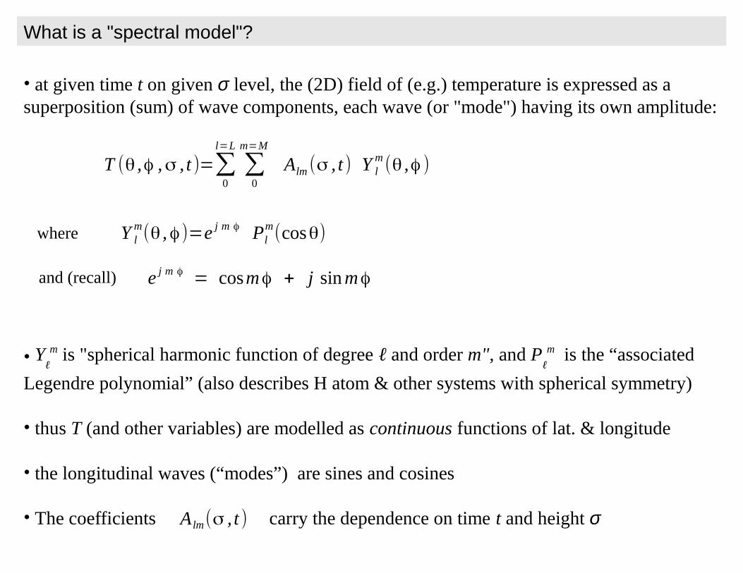
• at given time t on given σ level, the (2D) field of (e.g.) temperature is expressed as a superposition (sum) of wave components, each wave (or "mode") having its own amplitude:

• Yℓ

m is "spherical harmonic function of degree ℓ and order m", and Pℓ

m is the “associated

Legendre polynomial” (also describes H atom & other systems with spherical symmetry)

• thus T (and other variables) are modelled as continuous functions of lat. & longitude

• the longitudinal waves (“modes”) are sines and cosines

• The coefficients carry the dependence on time t and height σ

T ( ,ϕ ,σ , t )=∑0

l=L

∑0

m=M

Alm (σ , t ) Y lm( ,ϕ)

Y lm( ,ϕ)=e j m ϕ Pl

m(cos)where

e j m ϕ = cosmϕ + j sin mϕand (recall)

A lm(σ , t )

What is a "spectral model"?

• T574 means 574 waves are carried

• wavelength of the shortest is 360o/574 = 0.63o

• grid model of corresponding resolution would require 2 gridpoints per each shortest

wavelength, so would have grid spacing 1/2 x 0.63o (~ 35 km in latitude)**

Number of Number of σ σ levels = levels =

Number of Number of waves =waves = T1534

**c.f. NOAA: “resolution 28 km (70 km for 2nd week)”

What is a "spectral model"?

2014

NCEP T62 Gaussian grid

• coordinate system for “physics” calculations

• no grid points at the poles

• at every time step, model dependent variables are interpolated onto the Gaussian grid for the "gridpoint computations" (parameterizations)

Parameterizations are computed on a “Gaussian grid”

Why still formulated in vorticity and divergence? (note: GSM is not subject to all the restrictions of the quasi-geostrophic model)

NCEP’s Global Spectral Model (ver. 11.0.6)

Why still spectral? (JDW's speculation)

• historical continuity (continuously evolving model)

• not subject to Courant condition (limiting time step)

• not subject to non-linear computational instability

• trivial to refine horiz. resolution when comput'l resources allow

• historical continuity (continuously evolving model)

• solid theoretical justification (QG paradigm) to consider vertical vorticity,

horizontal divergence, & geostrophic vorticity- and thickness - advection as

basic to weather development

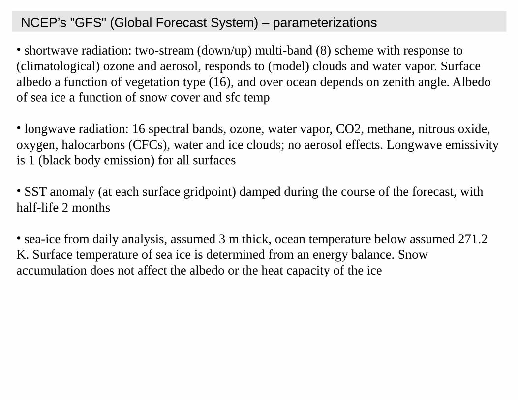
• shortwave radiation: two-stream (down/up) multi-band (8) scheme with response to (climatological) ozone and aerosol, responds to (model) clouds and water vapor. Surface albedo a function of vegetation type (16), and over ocean depends on zenith angle. Albedo of sea ice a function of snow cover and sfc temp

• longwave radiation: 16 spectral bands, ozone, water vapor, CO2, methane, nitrous oxide, oxygen, halocarbons (CFCs), water and ice clouds; no aerosol effects. Longwave emissivity is 1 (black body emission) for all surfaces

• SST anomaly (at each surface gridpoint) damped during the course of the forecast, with half-life 2 months

• sea-ice from daily analysis, assumed 3 m thick, ocean temperature below assumed 271.2 K. Surface temperature of sea ice is determined from an energy balance. Snow accumulation does not affect the albedo or the heat capacity of the ice

NCEP’s "GFS" (Global Forecast System) – parameterizations

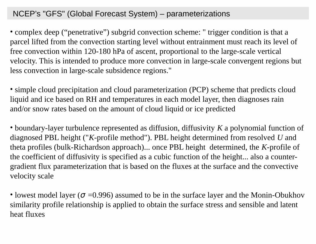
• complex deep (“penetrative”) subgrid convection scheme: " trigger condition is that a parcel lifted from the convection starting level without entrainment must reach its level of free convection within 120-180 hPa of ascent, proportional to the large-scale vertical velocity. This is intended to produce more convection in large-scale convergent regions but less convection in large-scale subsidence regions."

• simple cloud precipitation and cloud parameterization (PCP) scheme that predicts cloud liquid and ice based on RH and temperatures in each model layer, then diagnoses rain and/or snow rates based on the amount of cloud liquid or ice predicted

• boundary-layer turbulence represented as diffusion, diffusivity K a polynomial function of diagnosed PBL height ("K-profile method"). PBL height determined from resolved U and theta profiles (bulk-Richardson approach)... once PBL height determined, the K-profile of the coefficient of diffusivity is specified as a cubic function of the height... also a counter-gradient flux parameterization that is based on the fluxes at the surface and the convective velocity scale

• lowest model layer (σ =0.996) assumed to be in the surface layer and the Monin-Obukhov similarity profile relationship is applied to obtain the surface stress and sensible and latent heat fluxes

NCEP’s "GFS" (Global Forecast System) – parameterizations

• gravity wave drag

• snow cover from daily analysis. Precip falls as snow if temperature at σ=.85 is below 0oC. Snow mass prognostically from a budget equation that accounts for accumulation and melting. Snow melt contributes to soil moisture, and sublimation of snow to surface evaporation. Snow cover affects the surface albedo and heat capacity of the soil

• roughness z0 of oceans sensitive to wind, over land z

0 prescribed for 12 vegetation types.

Soil type and vegetation type data base, incl. vegetation fraction monthly climatology

• land surface processes: soil T and water content computed in two layers at depths 0.1 and 1.0 meters; heat capacity, thermal and hydraulic conductivity functions of soil moisture content. Climatological deep-soil temperature specified at 4 meters for soil, constant 272 K specified as the ice-water interface temperature for sea ice. Vegetation partially intercepts precipitation and re-evaporation. Runoff from the surface and drainage from the bottom layer are also calculated.

NCEP’s "GFS" (Global Forecast System) – parameterizations