NCAR-TN-33

Project ClambakeSurface Wind Analysisat Palestine, Texas

H. W. BAYNTON

NOVEMBER 1967

NATIONAL CENTER FOR ATMOSPHERIC RESEARCHBoulder, Colorado

I

I

iii

SUMMARY

A clam-shaped inflation shelter has been proposed for use during

launching of large balloons when wind speed exceeds 10 kt. Full use of

such a shelter would depend on forecasts of wind lulls lasting up to

10 min. Such forecasts would be feasible if the existence of coherent

eddies in the size range 0.5 to 6 mi could be verified. To determine

if such eddies exist, the Field Observing Facility of the National Cen-

ter for Atmospheric Research measured surface winds at 13 locations

within 5 mi of the NCAR Scientific Balloon Flight Station at Palestine,

Texas during October and November 1965.

Analysis of 102 hr of data collected on 12 days uncovered no evi-

dence of a coherent eddy structure in the required size range. Thus no

means of forecasting occasional lulls at the balloon base were apparent.

Wind bursts associated with cloudless cold fronts did appear to be pre-

dictable from a network of wind stations.

I

v

ACKNOWLEDGMENTS

Many people at both NCAR's Boulder Laboratory and the NCAR Scien-

tific Balloon Flight Station at Palestine, Texas, played an active part

in Project Clambake. However, the main burden of maintaining the net-

work of wind stations and carrying out the special observing program

was borne by Roy Eis, Lionel Johnson and James Starry. The study owes

the name "Clambake" to Jack Warren of the NCAR Scientific Balloon

Facility, who thought this appropriate to the project's close association

with the Clamshelter.

I~ ~ ~~~ ~ ~~~ ~ ~~~ ~ ~~~ ~ ~~~ ~ ~~~ ~ ~~~ ~ ~~~ ~~~~ ~~~~ ~~~~ ~~~~ ~~~~ ~~~~ ~~~~ ~~~~ ~~~ ~~~~~~~~~~~~~~~~~~~~~~~~~~~~~~~~~~~~~~~~~~~~~~~~~~~~~~~~~~~~~~~~~~~~~~~~~~~~~~

vii

CONTENTS

Summary . . . ... . . . .. .. . ................

Acknowledgments ........... .... ... ... v

List of Figures ............ ........ ix

THE WIND-SHELTER PROGRAM .......... .......... 1

DESIGN OF FIELD PROGRAM AND LOGISTICS .... ........ 2

SUMMARY OF FIELD TRIALS ..... .... ............ 4

RESULTS AND CONCLUSIONS . .................... 5

RECOMMENDATIONS .............. 8 .; . . 8

REFERENCES ..... ....... .... . .... . . . . 8

APPENDIXES . ............. ............ . 9

A. ISOTACH ANALYSIS OF SURFACE WIND DATA . . .......... 11

1. Introduction ...... .. . 11

2. Data Processing ........... 12

3. Analysis by Isotachs .... ......... . 13

4. Other Approaches ........ ....... . 16

5. Conclusion ...................... 17

B. ISOCHRONE ANALYSIS OF COLD FRONTAL PASSAGES ........ 19

1. Introduction .............-.. 19

2. The Analysis ................ 19

3. Discussion . .... . . * 20

FIGURES . .............. ........ . . . 21

I~~~~~~~~~~~~~~~~~~~~~~~~~~~~~~~~~~~~~~~~~~~~~~~~~~~~~~~~~~~~

ix

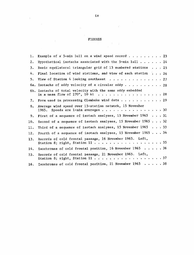
FIGURES

1. Example of a 5-min lull on a wind speed record ......... 23

2. Hypothetical isotachs associated with the 5-min lull . . . 24

3. Basic equilateral triangular grid of 13 numbered stations .. 25

4. Final location of wind stations, and view of each station . . . 26

5. View of Station 4 looking southeast . .. . . . ... 27

6a. Isotachs of eddy velocity of a circular eddy . . ........ 28

6b. Isotachs of total velocity with the same eddy embeddedin a mean flow of 270°, 10 kt .. . . . 28

7. Form used in processing Clambake wind data .. ......... 29

8. Average wind speed over 13-station network, 15 November

1965. Speeds are 1-min averages ................ 30

9. First of a sequence of isotach analyses, 15 November 1965 . . 31

10. Second of a sequence of isotach analyses, 15 November 1965 . . . 32

11. Third of a sequence of isotach analyses, 15 November 1965 . . 33

12. Fourth of a sequence of isotach analyses, 15 November 1965 .. . 34

13. Records of cold frontal passage, 16 November 1965. Left,Station 8; right, Station 11 ................ .. 35

14. Isochrones of.cold frontal position, 16 November 1965 . .. . 36

15. Records of cold frontal passage, 21 November 1965. Left,Station 8; right, Station 11 ............. ..... 37

16. Isochrones of cold frontal position, 21 November 1965 . . . . . 38

I

I

1

THE WIND-SHELTER PROBLEM

Successful launching of large balloons, not usually difficult in

winds of less than 10 kt, becomes increasingly difficult and uncertain

as wind speed increases. Winds greater than 15 kt cause considerable

difficulty: launching failures may be catastrophic, destroying a one-

of-a-kind balloon or an expensive payload. In practice, balloon

launches are planned for days promising winds below 10 kt, which is

considered a rule-of-thumb critical wind speed. If winds are not light

at the right time it may be impossible to carry out a mission planned

months in advance. One of the considerations in selecting Palestine,

Texas as the launch site for the Scien-tific Balloon Facility of the

National Center for Atmospheric Research (NCAR) was its characteristic-

ally light winds.

It was suggested that if balloon inflation were carried out in a

large shelter designed to open like a clam and rotate its closed side

into the wind, a short 1- to 10-min interval of light wind (less than

10 kt) might be sufficient for launching. Design studies for such a

structure were performed by NCAR, and a clam-shaped inflation shelter,

which became known as the Clamshelter, was proposed.

While detailed engineering of the Clamshelter progressed and esti-

mates of construction costs began to solidify, debate on the purely.

technical merits of the Clamshelter went on. Proponents of the Clam-

shelter argued that it would make inflation and launch possible despite

adverse wind conditions, that totally new operational techniques would

inevitably evolve, that more balloons could be launched, that more re-

liable flight schedules would be possible, and that, as a consequence,

experimentation by scientific ballooning would find wider use. Oppon-

ents of the Clamshelter argued that current launch techniques were

meeting the needs of interested scientists without undue delay, and

that the proposed Clamshelter would not remove the more serious problem

of interference by strong westerlies at float altitude during extended

2

periods in winter. They also maintained that more traffic could behandled, if necessary, by duplicating some of the existing facilities

at Palestine. In any case, the Clamshelter would be useful only if thewind, having dropped suddenly below 10 kt, would remain reliably calm

for the few minutes necessary to launch.

The last of these arguments could be answered if the feasibility

of 10-min wind forecasts could be demonstrated, and if 5-min lulls,

such as that shown in the wind trace of Fig. 1, could be predicted. Ifthe lulls were purely random events, their prediction would be out of

the question; but if they were the result of moving wind-speed fields

like that shown in Fig. 2, prediction might be possible.

DESIGN OF FIELD PROGRAM AND LOGISTICS

The NCAR Field Observing Facility was asked to determine the fea-

sibility of 10-min forecasts of wind lulls at Palestine. If such lulls

were not simply random events, they would probably result from eddies

embedded in the mean flow. Assuming a mean flow of 15 kt, the diameter

of 1- to 10-min lulls is theoretically about 0.25 to 3 mi, and the diam-

eter of the associated eddies is 0.5 to 6 mi.* (Perturbations in this

range are likely to be convective in origin.) If coherent 0.5- to 6-mi

eddies are a feature of the surface wind field, isotach analysis at

5-min intervals over a network of stations should show continuity from

map to map. The field program was designed to test this proposition.

Numerous decisions were necessary to determine appropriate network

size and the spacing and arrangement of the stations. The number and

type of wind systems were determined by the immediate availability of

12 AN/GMQ-12A wind systems, obtained on surplus. The lifetime of

dust devils, thunderstorms, and extratropical lows suggested that 30

min might be a typical life cycle for the size of perturbations under

* The diameter of the centers of high and low wind speed is about halfthe diameter of the embedded eddy, as illustrated in Fig. 6.

3

consideration. A 10-mi diam circle is large enough to provide a

30-min history.

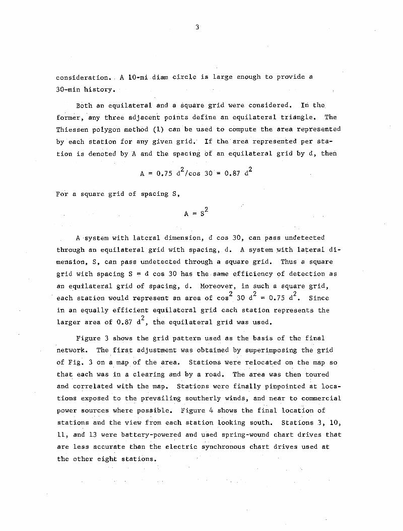
Both an equilateral and a square grid were considered. In the

former, any three adjacent points define an equilateral triangle. The

Thiessen polygon method (1) can be used to compute the area represented

by each station for any given grid. If the area represented per sta-

tion is denoted by A and the spacing of an equilateral grid by d, then

A = 0.75 d2/cos 30 = 0.87 d2

For a square grid of spacing S,

A S

A system with lateral dimension, d cos 30, can pass undetected

through an equilateral grid with spacing, d. A system with lateral di-

mension, S, can pass undetected through a square grid. Thus a square

grid with spacing S = d cos 30 has the same efficiency of detection as

an equilateral grid of spacing, d. Moreover, in such a square grid,2 2 2

each station would represent an area of cos 30 d= 0.75 d. Since

in an equally efficient equilateral grid each station represents the2

larger area of 0.87 d , the equilateral grid was used.

Figure 3 shows the grid pattern used as the basis of the final

network. The first adjustment was obtained by superimposing the grid

of Fig. 3 on a map of the area. Stations were relocated on the map so

that each was in a clearing and by a road. The area was then toured

and correlated with the map. Stations were finally pinpointed at loca-

tions exposed to the prevailing southerly winds, and near to commercial

power sources where possible. Figure 4 shows the final location of

stations and the view from each station looking south. Stations 3, 10,

11, and 13 were battery-powered and used spring-wound chart drives that

are less accurate than the electric synchronous chart drives used at

the other eight stations.

4

The operational plan specified a series of trials each lasting 4 hr

or more. Some night trials were planned to determine whether coherent

eddies were present only during convective heating. A chart speed of

12 in./hr was used on the wind recorders to permit accurate comparison

of 5-mintime intervals on separate records. Rawins, using a slow

ascent rate of about 200 ft/min, were released at 2-hr intervals and

tracked by an M-33 radar normally used at Palestine for tracking large

scientific balloons. One GMD-1 radiosonde flight was released during

each trial.

Although stations using commercial power could be kept operating

around the clock, battery-powered stations had to be placed in opera-

tion at the beginning of each trial. It was considered desirable to

inspect each wind station at 2-hr intervals during trials. The network

was, therefore, divided into two 6-station routes of 31 and 33 mi res-

pectively, requiring a normal driving time of about 90 min for routine

inspection and servicing. Two station wagons were rented and equipped

with two-way radio for this purpose. A four-man crew carried out the

field program.

SUMMARY OF FIELD TRIALS

Installation of wind systems began on 11 October and was completed

by 17 October. Heavy rain on 18 October interrupted a shakedown trial;

moisture shorted out most of the sensors. By 22 October repairs had

been made and nitrogen had been installed at all stations to exclude

water from the detectors. Figure 5 is a view of Station 4, showing the

plywood shelter for the recorder and electronic components, the nitro-

gen bottle, and the barbed-wire fence needed to exclude stock. On 22

October a 4-hr trial run was conducted without rawins or radiosondes;

adjustments suggested by the trial run occupied the next two days.

Immediately thereafter, a spell of generally fine weather settled

in with winds too light to be of interest. Although four 8-hr trials

were performed during this period in the hope that winds would increase,

5

the data were of little value. However, teamwork steadily improved.

The crew gained useful experience with the temperamental wind systems,

and ran a series of practice rawins and GMD radiosonde flights.

The collection of useful data began on 11 November. With continu-

ing favorable weather, eleven more trials were completed in the next

12 days, providing a total of 102 hr of data. Table 1 summarizes

this phase of the operation, showing the interval of each trial, the

time of release of rawins and GMD soundings, the height above ground of

the minimum potential temperature, the relative success of the surface

wind network, and the weather conditions.

The "% sfc wind data" column of Table 1 shows the number of

station-hours of data actually collected during a trial, expressed as a

percentage of the possible station-hours if each of the 12 wind

systems had functioned perfectly. The unreliability of the GMQ-12A

wind system is well illustrated by the drop in percentage of collected

data between 18 and 20 November. Six different types of malfunction

contributed to the loss of data on 20 November.

RESULTS AND CONCLUSIONS

Wind speeds at the 13 stations (12 network stations plus the

permanent balloon-base station) were plotted on a base map of the area.

Isotachs were drawn, locating the centers of high and low wind speed.

Appendix A describes the procedure in detail. Maps were prepared at

5-min intervals to show if continuity existed from map to map. Conti-

nuity would be expected if the centers of high and low wind speed were

caused by eddies embedded in the mean flow. Figure 6 illustrates the

kind of isotach pattern that would result from a circular eddy embedded

in a mean flow of 270 , 10 kt. In the illustration the eddy has a cen-

tral 4-kt velocity that decreases linearly to zero at 2 mi from the

center. The isotachs show a center of light 6-kt winds and a center of

stronger 14-kt winds. If the eddy persists and moves with the mean

TABLE 1

SUMMARY OF OPERATIONS, 11-23 NOVEMBER 1965

(All times local standard)

Time of Release Height Min.Pot.. Tmp. % Sfc

Date Trial Period (Rawins) (GMD) (m) Wind Data Weather

11 Nov. 1030-1600 1103 1500 1345 260 78 Brkn middle cld; aftn RW

12 " 1000-1600 1108 1520 1331 475 90 Lo ovc bcmg clear at noon

13 " 0800-1600 0840 1036 1504 1313 sfc 92 Lo ovc bcmg sctd at 1400

14 " 1100-1900 1117 1602 1802 1408 825 92 Lo ovc bcmg clear by 1600

15 " 1200-1800 1238 1729 2115 1419 1075 83 Lo ovc bcmg brkn Ci withsctd Cu by 1430

16 " 1200-2400 1254 1734 1953 1419 1025 92 Brkn Ci

17 " 0400-1200 - -- -- - -- 100 Brkn Ci

17 " 1200-2000 1249 1740 2004 1415 680 97 Brkn Ci

18 " 0400-1600 0738 0929 1102 1529 sfc 99 Ovc middle cld1334

20 " 0800-1800 0839 1045 -- 1442 915 73 Lo ovc bcmg sctd by 1500

21 " 0730-1730 0814 1016 1629 1311 1025 67 Vrbl brkn to ovc layers SC

23 " 0800-1630 0809 1103 1531 1337 650 88 Sctd Ci

7

270° 10-kt flow, in 15 min a lull ought to occur at P1 and a period of

stronger winds at P2.

No such sequence of events was observed in the hundreds of maps

prepared from the 102 hr of data. Although centers of high and low

wind speed were features of the isotach patterns, they simply appeared

and disappeared without any evidence of being advected by the mean flow

or of moving in any regular way. There was no evidence that detailed

knowledge of the wind field within 5 mi of the balloon base would en-

able prediction of lulls of less than 10 kt during periods of generally

stronger winds.

At times it is as important to predict sudden increases above 10 kt

as to predict lulls. On two occasions sudden increases were observed

during the passage of dry cold fronts. Appendix B contains an analysis

of these two frontal passages. Not only did the fronts move across the

network in a very regular way, but also the fine structure of the wind

trace was remarkably:similar at each of the 13 stations. Both cold

fronts passed through on days otherwise suitable for balloon launching;

frontal zone disturbances lasted less than an hour. There was

no associated cloud to warn of the approaching front. A network of wind

sensors with remote recording at the balloon base would provide a

feasible warning system.

Two main conclusions emerge in response to the primary objective

of the study.

1. A small 102-hr data sample taken over a network of 13 stations

on 12 days in the fall season gave no evidence of a coherent

surface wind structure in the required size range. No means

of forecasting occasional lulls at the balloon base were found.

2. Wind surges associated with cloudless cold fronts moved regu-

larly and retained their fine structure during the time required

to traverse the 10-mi diam of the network.

8

A serendipitous finding of the study was that useful inferences

about thermal structure in the surface layer can be drawn from precise

balloon tracking. Details will be published separately (2).

RECOMMENDATIONS

If it were desirable to warn of the approach of cloudless cold

fronts, a network of wind sensors north and northwest of the balloon

base would serve the purpose. Wind systems such as those of the new

Beckman and Whitley design could transmit wind information by telephone

lines to a recorder at the balloon base.

REFERENCES

1. Huschke, R. E. (ed.), Glossary of Meteorology, American Meteorolog-ical Society, Boston, Mass., 1959, 579.

2. Baynton, Harold W., "Stability inferences from precision rawins,"accepted for publication in Mon. Wea. Rev. 96(1), January 1968.

9

APPENDIXES

I

\~~~~~~~~~~~~~~~~~~~~~~~~~~~~~~~~~~~~~~~~~~~~~~

11

APPENDIX A

ISOTACH ANALYSIS OF SURFACE WIND DATA

1. INTRODUCTION

The network of wind sensors consisted of the permanent aerovane

mounted 80 ft above ground at the Palestine Launch Site, and 12 portable

GMQ-12A wind systems equally spaced around the aerovane within a 10-mi

diam circle. The GMQ-12A's were mounted 10 ft above ground in open

areas that could be reached by car. The numbering of the stations is

shown in Figs. 3 and 9.

Prior to each trial the technicians servicing the wind network

started stopwatches exactly on the half hour as indicated by the WWV

time signal. With this time base it was possible to specify start-up

time of each station to an accuracy of a few seconds. The WWV time

check was repeated prior to each service trip during a trial, and time

checks entered on each chart as part of the station inspection. During

an 8-hr trial there were normally three time checks in addition to the

start-up and shut-down times. This extra care made possible the time

matching of wind records to an accuracy of a few seconds.

Homogeneity of data is a matter of concern in any network. The

assorted differences present in Project Clambake are enumerated and

discussed below:

a. The starting speed of an aerovane is about 2 kt, that for a

GMQ-12A is 0.5 kt. Above 5 kt, which corresponds to the wind

regime under study, the difference becomes unimportant.

b. The wind is stronger at 80 ft, the height of the aerovane

than at 10 ft where the GMQ-12A's were mounted. The simple

standardizing procedure described below (Section 2) corrects

for this small difference as long as the air is well mixed.

However, at night there were instances of calm winds at 10 ft

increasing to about 8 kt at 80 ft. At such times the aerovane

12

is clearly not represented by the network, and isotach

analysis becomes pointless.

c. Despite great care in the selection of open sites, differences

in exposure were inevitable. Station 5 offered the poorest

exposure, as it was located in a slight hollow with a few

trees to the south. These differences were nullified by the

procedure described below (Section 2) for standardizing the

data.

d. The use of battery power at four GMQ-12A stations was more of

an inconvenience than an inhomogeneity. Direct current from

a lead-acid battery was converted to 60 cycles ac and stepped

up to 117 V. As the battery drained, the voltage dropped,

sometimes to the point where the speed transducer, a light

chopper, would cut out between service trips. Equally incon-

venient was the use of spring-wound chart drives at the battery

stations. Chart speed might vary by 3 per cent from the nominal

12 in./hr. Moreover, chart speed varied slightly from trial

to trial and during trials. Time matching of these records

was consequently a tedious job.

2. DATA PROCESSING

Charts from the 13 wind recorders were processed in sets corre-

sponding to trials. The first step in this procedure was a quality-

control scan of each chart for gaps in the record, failures of chart

drive, and errors in entering time checks. With the four mechanical

chart drives it was also necessary to compute the exact chart speed for

each interval between time checks and then insert exact time lines on

the charts.

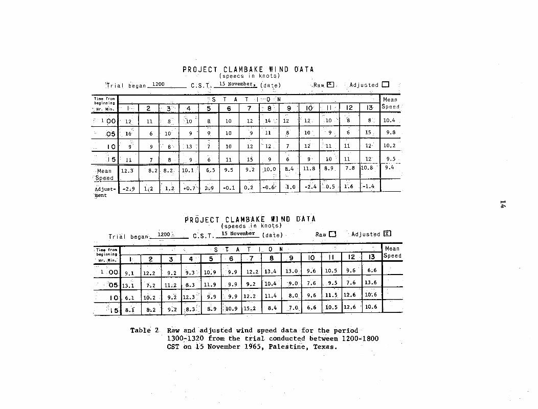
The next step was the compilation of raw data on the form shown in

Fig. 7. The mean value for the first minute of each 5 min was read and

entered, to the nearest 5° for direction and the nearest whole knot for

speed. From these raw data, mean speeds for each station for-the entire

trial were computed and entered on the last line of the form. The mean

13

speed of all 13 stations was entered for each 5-min period, and in the

lower right hand corner the mean of all 13 stations for the entire

trial was entered. The upper half of Table 2 contains a 20-min sample

of raw data (speeds only) from the 15 November trial. The mean speeds

for the stations are based on the entire trial; 9.4 kt is the trial

mean for all 13 stations.

Each station mean was then subtracted from the trial average of

all 13 stations to give the adjustment factors shown in the sixth row

of Table 2. A set of adjusted wind speeds was obtained by adding the

appropriate adjustment factor to each of the raw data entries for a

particular station. The lower half of Table 2 shows the adjusted wind

speeds corresponding to the raw data in the upper half of the table.

The assumption underlying this procedure is that, aside from local fac-

tors, each of the 13 stations should have the same mean wind for the

duration of the trial. Differences between stations that show up at

any time in the adjusted data are then the result of the small-scale

disturbances which were the subject of the investigation.

3. ANALYSIS BY ISOTACHS

To find suitable periods for analysis the 13-station mean was

plotted against time, as shown in Fig. 8. Data from 15 November are

again used as an illustration. It can be seen that, aside from short-

term fluctuations, wind speed was uniform until 1540 when the diurnal

decrease began. The period 1200-1540 should therefore be well suited

to isotach analysis for traveling eddies.

Adjusted wind speed and observed wind direction were then plotted

for each station on maps of the area for successive 5-min times, and

isotachs were drawn at l-kt intervals. There was a conscious attempt to

achieve continuity of closed centers of high and low wind speed by ex-

trapolating at the edge of the network and between stations.

A representative sequence of these maps appears in Figs. 9, 10, 11,

and 12. This sequence is based on the adjusted data for 15 November

that appear in the lower half of Table 2. Adjusted wind speed is shown

PROJECT CLAMBAKE WIND DATA(speeds in knots)

Trial began 1200 C.S T. 15 November, (.date) .Raw E]. Adjusted El

Time from ,S T A T I 00 ;N Meanbeginning

Hr. Min. 2 ; 3- 4 5 6 7 -8 9 10 .11 12 13 Speed-. . - _ -. .- :. -

1 00 12' 11 8 8 8 10 12 14 12 12 10 8 8 10.4

05 16" 6 10- 9 9 10 9 11 8 10 9 6 15: 9.8

10 9 9 8 13 7 10 12 12 7 12 11 11 I 12 10.2

1 5 11 7 815 9 6 11 15 9.5

'Mean |12.3 8.2 8. 2 10.1 6.5 9.5 9;.2 10.0 89 .8 1.8 9.4S p ee d _ _________ _ _- —— —

:- 1 .: :. .

Adjust- -2.9 12 1.2 -0.7 2.9 -0.1 0.2 6- -0.6 1. -2.4 |0.5 1.6 -1.4Im'ient

PROJECT CLAMBAKE WI ND DATA(speeds in knots)

Trial began 1200 C.S.T. 15 November (date) Raw Adjusted X

-Time from - S T A T 1 0 N ' S'_ _A T Meanbeginning :' ... — i " -·

H..Min. : 2 3 4 5 6 7 8 9 10 !1 12 13 Speed

1 00 9.1 12.2 9.2 .3 10.9 9.9 12.2 913.4 13.0 96 10.5 96 .6 6.6

05 13.1 7 .2 11.2 8.3 11.9 9.9 9.2 10.4 9.0 7.6 9.5 7.6 13.6 _

1 0o 6.1 10.2 9.2 12.2 .4 8.0 .6 11.5 12.6 10.6

5 8.1 8.2' 9:.2 .8.3. 8.9 0.9 15.2 8.4 7.0 6. 6 10.5 12.6 10.6

Table 2 Raw and adjusted wind speed data for the period1300-1320 from the trial conducted between 1200-1800CST on. 5 November 1965, Palestine, Texas.

15

above and to the left of the station circles, and observed wind direc-

tion above and to the right of station circles.

Overcast stratocumulus present at noon had become broken by 1300

CST, when the map sequence begins. As the afternoon progressed the

broken stratocumulus gradually changed to scattered cumulus. Broken

thin cirrus clouds were also present throughout the trial. A rawin

launched'.at 1238 CST showed superadiabatic (convective) conditions

through the lowest 600 m , The method used to draw this inference con-

cerning temperature structure from rawin flight data is described in

(2). The mean wind within the convective layer was 2090, 19 kt. Direct

temperature measurement by rawinsonde at 1419 CST indicated superadia-

batic conditions through the lowest 1075 m and a mean wind within the

convective layer of 2070, 22 kt.

It is evident that convective conditions were present during the

20 min illustrated in Figs. 9, 10, 11, and 12, and that convective

eddies embedded in the mean flow should move generally from the south-

southwest at a speed of 20 kt. If the centers of high and low wind

speed shown in the four figures are the result of embedded eddies, they

should show the same motion.

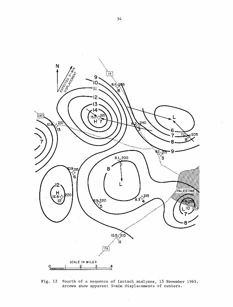
A vector showing the expected 5-min displacement by a 208 , 20-kt

wind is drawn in the upper left corner of Figs. 9, 10, 11, and 12. The

apparent 5-min displacements of the centers are shown with arrows.

There is a striking lack of good agreement with the expected displace-

ments. In Fig. 11 there are two possible displacements for the lows

situated over Station 1 and northwest of Station 2. In Fig. 12 there

are alternate displacements for the high at Station 7 and the low near

Station 9. Some displacements imply speeds as high as 50 kt. In short,

there is no evidence that the successive isotach patterns of Figs. 9,

10, 11, and 12 can be related by the advection of small convective dis-

turbances in the mean flow.

It should be emphasized that this 20-min illustration from the 15

November trial is entirely representative of the results obtained from

the other trials.

16

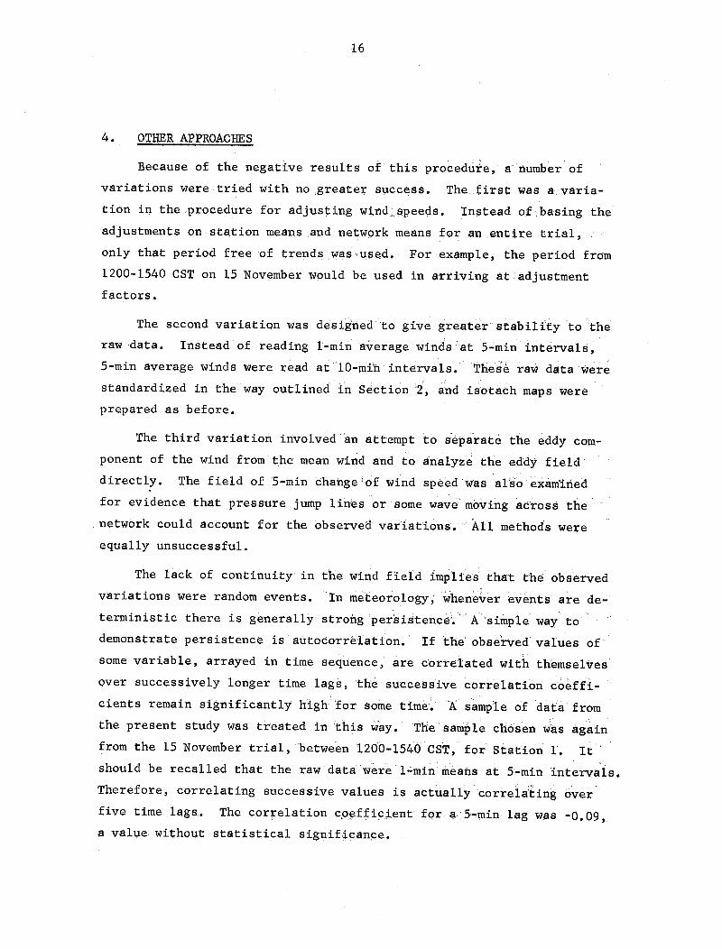
4. OTHER APPROACHES

Because of the negative results of this procedure, a number of

variations were tried with no greater success. -The.first was a varia-

tion in the procedure for adjusting wind.speeds. Instead of basing the

adjustments on station means and network means for an entire trial,

only that period free of trends was-used. For.example, the period from

1200-1540 CST on 15 November would be used in arriving at adjustment

factors.

The second variation was designed 'to give greater stability to the

raw data. Instead of reading i-min average winds at 5-min intervals,

5-min average winds were read at 10-mi'h intervals. These raw data were

standardized in the way outlined in Section :2, and isotach maps were

prepared as before.

The third variation involved'an attempt to separate the eddy com-

ponent of the wind from the mean wind and to analyze the eddy field

directly. The field of 5-min changeof wind speed'was also examined

for evidence that pressure jump lines or some wave moving across the

network could account for the observed variations. All methods were

equally unsuccessful.

The lack of continuity in the wind field implies that the observed

variations were random events. In meteorology, whenever events are de-

terministic there is generally strong persistence.' I A'simple way to

demonstrate persistence is autocorrelation. If the observed values of

some variable, arrayed in time sequence, are correlated with themselves

over successively longer time lags, the successive correlation coeffi-

cients remain significantly high for some time. 'A sample of data from

the present study was treated in this way. The samp le chosen was again

from the 15 November trial, between 1200-1540 CST, for Station 1. It

should be recalled that the raw data were 1-min means at 5-min intervals.

Therefore, correlating successive values is actually correlating over

five time lags. The correlation coefficient for .a5-min lag was -0.09,

a value without statistical significance..

17

5. CONCLUSION

Isotach analysis, as described above, gave no evidence of a coher-

ent wind structure in the size range 0.5 to 6 mi. Rather, the isotach

analyses and the autocorrelation of wind speeds imply that occurrences

of 1- to 10-min lulls are random events.

(~~~~~~~~~~~~~~~~~~~~~

19

APPENDIX B

ISOCHRONE ANALYSIS OF COLD FRONTAL PASSAGES

1. INTRODUCTION

Appendix B deals with the forecasting of bursts of strong winds

during periods of light winds. Among the causes of such bursts, are

cold fronts, squall lines, pressure jump lines, and thunderstorms. Two

cloudless cold fronts accompanied by stronger winds were followed across

the network during the Clambake field program. Bursts of strong winds

caused by other factors were not observed.

2. THE ANALYSIS

The first cold frontal passage was observed on 16 November 1965.

Although weather maps for the day showed a cold front approaching from

the northwest, there was no associated cloud to mark its position. Its

passage at all 13 stations was readily pinpointed by an abrupt increase

in wind speed and shift of the wind to northerly. A few minutes after

passage the wind began to decrease. Figure 13 gives the wind

trace at Station 8 as the front entered the network, and at Station 11

as it passed beyond the network. The similarity of the traces is

striking.

Times of frontal passage were plotted on the map shown in Fig. 14

and isochrones drawn to show the position of the front at 5-min inter-

vals. This front moved south-southeastward at a speed of 13.7 kt.

The second cold frontal passage was observed on 21 November 1965.

Once again the frontal passage occurred during the early evening and was

unmarked by cloud. Wind traces from Stations 8 and 11 are shown in

Fig. 15. Isochrones of frontal position are drawn on Fig. 16.

This front moved southeastward at 12.8 kt.

20

3. DISCUSSION

Both fronts resulted in a burst of stronger winds on a day that

was otherwise ideal for launching balloons. The fine structure of the

wind speed trace was remarkably persistent during the half hour it took

the front to cross the network. Forward motion of the front was consis-

tent enough to suggest that quite accurate predictions of the associated

wind burst could be made from a network of wind stations northwest of

the balloon launch site.

21

FIGURES

J

l

v~~~~~~~~~~~~~~~~~~~~~~~~~~~~~~~~~~~~~~~~~~~~~~~~~~~~~~~~~~~

H.

•f 30

XW 25Iw 0

"0__0800 081_0 0820 0830 0840 0850 0900

u, to~TIMED.0

Z 5 .

0800 0810 0820 0830 0840 0850 0900

'i3., TIME

24

8 I0 12 14 16

LIGHTWINDS

WINDDIRECTION

Fig. 2 Hypothetical isotachs associated with the5-min lull illustrated in Fig. 1.

25

8N

/ N

13 / 2.85 mi , \9

7 2

:~~~~~~~~~~~~~~~~~~~~~~~~~~~\I , Launch Site -6 I ..... ;;.. ...... rz...............-.. ... . .~ . ...ii..

^ ^ ^I mi 3 ''' :::::;.::

' ::::::::::: ::::.:::

o~~~~~~~~~~~~~~··· 0· 0·

-'NO - .......:::

-~~~~~~~~~~~~····· ·· ·. ~~:::: r

Fig. 3 Basic equilateral triangular grid of 13 numberedstations centered on Palestine launch site.

26

N * PROJECT CLAMBAKE

rj', Fig. 4 Final location of wind*.,:i~i„„„i„ „.„„„ ___stations, and view of eacht* station, looking south.

BALLOON LAUNCH0_ 2!3 _SITE

.....2

liii1.... :'"" ...

.......... .................... ............. ...... ............ ..... ..... ... ............ ............ ..... ....... ......

.............. -............. ........... -..................... ............ ....... .... .............. ............ .. ...... .......... .......... ............. ....... -........... ................. ... .......... .. .... .......... ................ .............

........... ............ ........ .... .. ..... ........................... ...................... ....... ........................ ..

...... ....... ........ ... ........I....'' � :: � X .: ............................. ..... .......

................ .. .................... :::::: � -1.1. .1- 1 -1- 1.1 I I .�: :::::::.: X .: : :::: ::::::: :::;..: I . .......... ................ ........................ ... .. ...... .............................. ........... ....

...... ...... ............ ............. .. ....... ................. ...................... ............ ................ .. ... ........... -.......... ........... .. ................... ......... ........................ ............ ........ .. ........ ........................ ............-

............. ::;::::::. . ::::X ;�X : :: : ! ; :: �- --- , " .".......... ..........I.......... ... ........... ..............

................ �: ........... .................... ........................... ... .......... ...... .... ............. ............. ........... .. .- ........... ............... .. .... ...... .. .- .. ........ .......... ......... .... ..........................X ........... .............

............... ... ........... .. .............................. X ., ................................ ....... .... . ........... .......... ........ ..... ..........-

.............. ... ..... .... ...............': :.. .... ...... :111, .:::: .:. X - I.... ......... .......... ...... ........... .......... ......

............. .... .......... ......

,:: ... ...... ....... ... .... ............. . ..............

......... .. .......... .......... ...

...... ...... ......- ...... ......... .. ............... ........

......... .......-. .................... .. .......... ... ..................... ......... .......................................... ... .111. .. �: ............... .... .... ............ ................................... ................ ............................. - ... .... ..... .... . ..............

................... ... ...... ....X : X : ................................. .......... ....... .............. ........... .......... ......-................. ........ .. ..... .......

; ::::X :: ::: ::::::;::::::: : :: :;::: :::::::::::::::::: :: X � -;,.",-_-_-.-. .; - I.., -................ -P................ ........... ... ............ ......... ... ....... ........ ..... ........ .... ............ ...... ....... ....... ... ..........

........ .... .. .. ... . ............... ....... ....... ........ ...... ......................... .................. ..... .. ...... ......... ....................... , " % :: ::::::::.

...... ...... ... ........ .................... ............ ...... ...........-

.......................... .......... ........ .......................... ....... ................... .......... ...................... ........... ................ ....... .... .... ....... ........... ...................... ................. .... .... . ............ ...................... ..... .......... .... ... ............... ............................ .....................-........ .. ..

.......................

....... . .... .... ......X . X ...................... .................................. .......................... ................... . .......... .. ......... ....... ............................. .............. .-..........

............ ....... .... . .........-................. ........... ..... ... ... .. .............. Ifa i ,::: : �::X I::::::::� .... ....... ............ ..........: : .,:: ; ................... .............. ...... ................

.......... .............. ............. .... .... .............. .............. ........ ..... ......... I................... ....................... ..... .... ........ ..... ................. .......... .......... ....... ..... ..... ....................................... � � -% : -. .......... ....

......... ... ... ....... ........... ............... ...................... ... ...... .. ......... . ................ . ................... ..........

....................... ........... ............... .......... ... .... .......... ................ .............1: I.I......,, .. -:. : : : ' : :.: ...... ......... ........... ......... ...

.......... ........... ............. ............ ...... ................................. .. .......- ....... ... ........ ................ .. ........................................... .......... .................... .............. ...................... ...........-

................... ......... ........ ......

............... .............. .. .............. ................ . ............... .......... ....................................... .... ....... ... ... ............

.... ............. ... ....... ........... ........... .......... X ............. ................... .............. .................... ........ ................ ..... .... ............... ... ............ ............. ........... .............

.......... ........ .... .... .......... ......... ................. .... ................ ... .........

......... .. ...... ........ ............ .......................... ............ ...... .... .. ... .... ....................- ............. ... ...................... .... .... .. ................... . .......................... . .. ............... ...... .................... ... ..... ....... ........... .............................. ............ ......... ...........

...... ...... . ..... ............... ........ .................. .... ......... ............................... ..................... .............. ..... ........... .............. ..... ....................... ....... ......

......... .............

....... ....... ..............X X .............. . .............. ............... ...... . .......... ....................................................... .. ........

...... ..... ............ ....... ............ ................... .. .... ........ ............................... ...... ...... ... ............ ...... ......

.......... ............ ........... ............... .................... . .......... ...................

.. ........ - :X .:: X X ..................... ..... .............. .. ........... ................ ...... ......

............. ....... .. .............................. ................. ........... ..................... ................

.......... ....... ..... .......................................

.... .... ... ........... . .......... ........... .... ..

... ............ . ............. ........... ........ .... ..................... -..................

..................I........ .... . ....... ....... ... ... ... ... . .......... ....... i::::!:!: X ....... .....

..................... ...... .......... ... - .............

.................. ........ ... .................. ......................... .......... . .........

.......... ...... .......... ...................................................... ... ........................ ............... .... ............... ...........

............. .................................... .................. ............. ....................... ............. ............................... I I :

.......................... ......................................... .. ............................. .. .... .......... ..........

... ....................................... .................................................. ............... .... . ...........

................... ... �X : . ..................... .. ................. .. ..... .........I.............................................. .............. ....

......... .. ...................................... X ..... ................................. .. ........ .............. ...... ...............

....................... .. .....

......................... .................................. ..............

...............................

....... .......... .................

.................

2.,v �,*�iw i��,

..............

GiulianiWill............

............. .. .. .....

. .... ......

...............

....... ....

......... .............. ....

..................... ... .............. ................................................. .......................... .............

.................................

.... ............ ... ............ ........ ..... ....................... ...

28

SCALE IN MILES0 1 2 3

1 X I I 1 : -_

Fig. 6a Isotachs of eddy velocity of a circular eddy.

_ \

/ 9^PI

1 4 -I X-3

II I

Fig. 6b Isotachs of total velocity with the sameeddy embedded in a mean flow of 270 ° , 10 kt.

29

PROJECT CLAMBAKE WIND DATA(speeds in knots)

Trial began ___C.S.T. (date) Raw f Adjusted aTime from S T A T I 0 N Meanbeginning

Hr. Min. 2 3 4 5 6 7 8 9 10 I 12 13 eed

05

0 ___

15 .. ___

20____

25_____

30 _

35 ____

40_____

45____

50 ____

55 _____

00_____ ___ __

05__

I0

15

20

2530 ______ ___

35____

40

45

50

55

00

MeanSpeed

14

co

12-

0 0

C(D

Xa,_t.n fD

(D W

I I- I

CENTRAL STANDARD TM E

CD

1200 1300 1400 1500 1600 1700 1800

CENTRAL STANDARD TIME

31

8

II

X~ ' '···12.2 1240 '- 1.2· \ 13\18 2.2 240 ~13 210

`9.2 235/IO\^~~ V~9 110 I O

PALESTI NE:::

96210 930

12 10.923 4 .2

10.5 195

32

~N /~10.420

I L \ \ \ \// / / ^^ I8 ~:PALESTINE

9~~~~/ \35 II

SCALE IN MILES

8~~~~~~~~~~'

0 8 23324

Fig. 10 Second of a sequence of isotach analyses, 15 November 1965.

Arrows show apparent 5-mmn displacements of centers.

33

Ne

*~'~1 21 0

""-.

SCALE IN MILES0 1 2 3 4

Fig. 11 Third of a sequence of isotach analyses, 15 November 1965.Arrows show apparent 5-min displacements of centers.

/ / ~~~~V~~ ""t'-~.9~ '.;~--~~I

34

3 *

>0

SCALE IN MILES0 1 2 3 4

Fig. 12 Fourth of a sequence of isotach analyses, 15 November 1965.Arrows show apparent 5-min displacements of centers.

10 5 `21~~~~~~.

35

WIND SPEED WlNP SPEED

-to= = =^ = =&=== ^ = = == = == ^ = ^ •_.(

_- l _ -O. O-_ tD- _= =-_ _-=_ . _r "•r=-_.

O LO S S at.

~ i L ^ : — 0 0 — — 0 ' 0 — — I I I — — F t---.=

i E o ~~Cto=ioo 0 ]10 t e S033d' GNIM a33dS aNIM

WIND SPEED WIND SPEED

_ _ _~~~~~~. _ _ 04. N

~~~~~~~~~~~~~~~~~~~~~~~~~~~~C M

i', I~i:~ i 1? .1!1L' 1,11 ili C\,'i : ii ' ,, , -,, 'L Ol i: : iii i |l ' i i

'I,. , ,51i i i ,l!11$i OyO i' NyU311 1 111''~~ll~lilII I I1 1— 1—— -I — — —~

,%'~.i., i':',L~."-':il,::''~,, ..... : '-:li, :..,.':,' .1I .".J i.-'J lll~lii [ii " ~'.=.=.:= .[.. .,.= I

.~~~~~~~ -

*_ ..... -L .-i_-- ................ ... -'... ., .. i, .1 ' .,,_,,,,,,;*

ml~llJJ , J ll 'l~lll lldll lll lIQl~ll'IIBIN.'IE ....... . .1-.

m,~ ~ ~ C~U= ~ ~ i..q -M- -

_____~~~~~~~~CI _ 0 _m

J - _~~~~~~~~~

.. ~ .,,i

======== ^ — — — == ==^== ^ =-— — —=----— ~.-

i33dS CNIM C33dS CNIM

-~~~~~~~~~~~~0Fig~~~~~~~.: 1 Reo dso cldfonta pasg,1 ovebr16..

Left, Staio 8;~ rih.SainI. ~

36

1719'

:

1720

1725~. *. /

^ ^ 1725 17 I73Q...... 2

1730 9

:-;'7 ..............

Fg17 ~1474ohoe2f 0odfotlpstin+6Nvme 16.

0 I 2 3 4................. _

Fig. 14 Isochrones of cold frontal position, 16 November 1965.~~~~~~~~~~~~~~~~~~~~~~~~~......

37

WIND SPEED WIND SPEED

_ ~ ~ ~~~~~~~~~~~t _

=Z=—==^ ==— — F- = = _ — — : _ _— — _ _

1F F— — — — ==F == ^I rl _^ _= — —

_s _ r 7 7 ru 1x X X n_ ~~~~~~~~~~~~~l -4.

-^_ ̂^_ —o o— ——— -^^^ i ̂ ^^ ̂ ^^^^ • -^^_ -^_^_ •^^_ ^^^ —o o— ^ ^ ^^^^ r^^z ̂ ^^: ̂ _ r ̂ : nr=_ _ r ro r T I—o o ^

_Oi _ CIOC__=_O _O__33dS33dS GNIM 33dS NNII

Left, S 8$ rgt S

M~~~~~~~~~~~lr-lll|||ln||l-- il* AX11l~l~w 1|

I0 10U I ~ §I I l 1 k0

I ~ ~ ~ ~ ~ ~ ~ L= = .o Le)IIF'llIII11 111l1 1ll1111 l1 1i'1 1 ~~~~~~~~L _0 _ 4 ,, C, j 1 :1 as* 1** f-0 ;!11I s1{i 's*s IsX*XXEx

_C~~~~~~ r L. (, 1 .,, . ,M_ .,,r- 2n) ,.,,.

* _c

G33dS~ ~ ~ ~~1 C11NIM C333dSl CM111ll1 11|i iM'11 1111 111

'111|11 111|11 Ul ; B 1 11 1

0e 1ill«1lul= llll *-- 1 1 &E 1 i1 11 1

U~~~~~~~~~~~~-_w~f1w*|- .t' -_ |1_i.

|X . .L_ .w _ w,,^ s7it=_@1.* .................................... _

38

N

18

1845

y^ 1855 / -... / 1+ 7895 1900+846

13 2 11

1855

-^- ^^ ̂ 1915^^~~~~~~~~91

1900

^^ ^^ 1915 ^y^190

^~~~~~~~~~~~~~~~~~~~~~~~~~~~~~~~~~~~~~~~~~~~~~~~~~~~~~~~~~~~f ..........

I1859+6 1905

7923 4

"iiiiiiiii~~~~~~~~~~~~~~~~~~~~~~~~~~~~~~~~~~~~~~~~~~~~. ..... » ....

Fig. 16 Isochrones of cold frontal position, 21 November 1965.