NBER WORKING PAPER SERIES

PRODUCTION FUNCTION AND WAGE EQUATIONESTIMATION WITH HETEROGENEOUS LABOR:

EVIDENCE FROM A NEW MATCHEDEMPLOYER-EMPLOYEE DATA SET

Judith K. HellersteinDavid Neumark

Working Paper 10325http://www.nber.org/papers/w10325

NATIONAL BUREAU OF ECONOMIC RESEARCH1050 Massachusetts Avenue

Cambridge, MA 02138February 2004

Many aspects of this paper were inspired by the teaching, research, and guidance that we were privileged toreceive from Zvi Griliches. We thank Melissa Powell and especially Joel Elvery for excellent researchassistance, and we thank Kim Bayard, Gigi Foster, and Nicole Nestoriak for help in the construction of theDEED data set. Our long-term research with the data sets used in this paper has been supported by NSF grantSBR95-10876, the Russell Sage Foundation, and NIH grant 1-R01-HD43358-01A1. This paper reports theresults of research and analysis undertaken while the authors were research affiliates at the Center forEconomic Studies at the U.S. Census Bureau. It has undergone a Census Bureau review more limited inscope than that given to official Census Bureau publications. Research results and conclusions expressed arethose of the authors and do not reflect the views of the Census Bureau or the Public Policy Institute ofCalifornia. Results have been screened to ensure that no confidential information is revealed. This paper wasprepared for the NBER CRIW Conference “Hard to Measure Goods and Services: Essays in Memory of ZviGriliches.” The views expressed herein are those of the authors and not necessarily those of the NationalBureau of Economic Research.

©2004 by Judith Hellerstein and David Neumark. All rights reserved. Short sections of text, not to exceedtwo paragraphs, may be quoted without explicit permission provided that full credit, including © notice, isgiven to the source.

Production Function and Wage Equation Estimation with Heterogeneous Labor: Evidence from aNew Matched Employer-Employee Data SetJudith Hellerstein and David NeumarkNBER Working Paper No. 10325February 2004JEL No. J7, J3, J4

ABSTRACT

In this paper, we first describe the 1990 DEED, the most recently constructed matched employer-

employee data set for the United States that contains detailed demographic information on workers

(most notably, information on education). We then use the data from manufacturing establishments

in the 1990 DEED to update and expand on previous findings, using a more limited data set,

regarding the measurement of the labor input and theories of wage determination. We find that the

productivity of women is less than that of men, but not by enough to fully explain the gap in wages,

a result that is consistent with wage discrimination against women. In contrast, we find no evidence

of wage discrimination against blacks. We estimate that both the wage and productivity profiles are

rising but concave to the origin (consistent with profiles quadratic in age), but the estimated relative

wage profile is steeper than the relative productivity profile, consistent with models of deferred

wages. We find a productivity premium for marriage equal to that of the wage premium, and a

productivity premium for education that somewhat exceeds the wage premium. Exploring the

sensitivity of these results, we also find that different specifications of production functions do not

have any qualitative effects on the these results. Finally, the results indicate that the returns to

productive inputs (capital, materials, labor quality) as well as the residual variance are virtually

unaffected by the choice of the construction of the labor quality input.

Judith K. HellersteinDepartment of EconomicsTydings HallUniversity of MarylandCollege Park, MD 20742and NBERhellerst@econ.umd.edu

David NeumarkPublic Policy Institute of California500 Washington Street, Suite 800San Francisco, CA 94111and NBERneumark@ppic.org

1For a comprehensive review of the measurement of the labor input, see Griliches (2000, Ch 3).

1

I. Introduction

The measurement of the labor input in production functions arose as an important issue in the

middle of the 20th century, when growth accountants speculated that the large “residual” in economic

growth calculations might be due not to disembodied technical change, but rather due to mismeasurement

of the labor input. Since that time, many economists have implemented methods to try to measure more

accurately the quality of the labor input (and, when appropriate, its change over time).1 Recent advances

in the creation of matched employer-employee data sets have markedly improved our ability to measure

the labor input at the level of the establishment. These matched data sets contain detailed information on

the characteristics of workers in establishments, which can be used to model and measure the labor input

directly, accounting for the different types of workers employed in each establishment. Moreover,

estimates of the relationships between the characteristics of workers and their productivity can be

contrasted to estimates of the relationships of these characteristics to wages to test theories of wage

determination.

In this paper, we first describe the most recently constructed matched employer-employee data set

for the United States that contains detailed demographic information on workers (most notably,

information on education). This data set, known as the 1990 Decennial Employer-Employee Dataset (or

1990 DEED), is a match between the 1990 Decennial Long Form of the Census and the 1990 Standard

Statistical Establishment List (SSEL), which is created using address matching software. It is much larger

and more representative than previous matched data using the Decennial Long Form data. We then use

the data from manufacturing establishments in the 1990 DEED to update and expand on previous

findings, using a more limited data set, regarding the measurement of the labor input and theories of wage

determination (Hellerstein, et al., 1999). Finally, we examine estimates of some of the key characteristics

of production functions, and how sensitive they are to the specification and measurement of the labor

input.

We find that the productivity of women is less than that of men, but not by enough to fully

explain the gap in wages, a result that is consistent with wage discrimination against women. In contrast,

we find no evidence of wage discrimination against blacks. We estimate that both the wage and

productivity profiles are rising but concave to the origin (consistent with profiles quadratic in age), but

the estimated relative wage profile is steeper than the relative productivity profile, consistent with models

of deferred wages. We find a productivity premium for marriage equal to that of the wage premium, and

a productivity premium for education that somewhat exceeds the wage premium. Exploring the

sensitivity of these results, we also find that different specifications of production functions do not have

2For a complete description of the construction and evaluation of the data set, see Hellerstein andNeumark (forthcoming (a)).

3Work on the construction of the 2000 DEED is underway. Another national matched employer-employee data set currently under construction at the U.S. Census Bureau is a match between stateunemployment insurance records and ES202 data as part of the broader Longitudinal EmployerHousehold Database (LEHD) project. These matched data are very rich in that they contain observationson all workers in covered establishments (not limited to the one-in-six sample of Census Long-Formrespondents) and are longitudinal in nature. Until recently, these data could not be linked to detaileddemographic information on workers (and can only be linked to 2000 data), and do not cover all states(although they do cover some of the largest ones). In addition, the matching algorithm matches workersto firms rather than establishments, so that an exact match between workers and establishments can onlybe made when the establishment is not part of a multi-unit firm. For details, see lehd.dsd.census.gov. For a good example of how these data can be used, see e.g. Abowd et al. (2002).

2

any qualitative effects on the these results. Finally, the results indicate that the returns to productive

inputs (capital, materials, labor quality) as well as the residual variance are virtually unaffected by the

choice of the construction of the labor quality input.

II. The Construction and Evaluation of the 1990 DEED

A. Introduction

Fifteen years ago, data sets matching employees with their employers were virtually nonexistent.

Fortunately, since then matched employer-employee data sets have been created, first for other countries

and then more recently for the United States. Indeed, in the most recent volumes of the Handbook of

Labor Economics (Ashenfelter and Card, 1999), a full chapter is devoted to research using these data (see

Abowd and Kramarz, 1999).

This section of the paper reviews the construction and evaluation of a new U.S. matched

employer-employee data set, based on the Decennial Census of Population for 1990.2 The key innovation

in this data set – which we call the 1990 DEED (Decennial Employer-Employee Dataset) – is that we

match workers to establishments by using the actual written worker responses to the question asking

respondents to list the name and business address of their employer in the week prior to the Census.

These responses are matched to a Census Bureau file containing business name and address information

for all establishments in the United States. The resulting data set is very large, containing information on

3.2 million workers matched to nearly one million establishments, accounting for 27% of workers who

are Long-Form respondents in the Decennial Census, and 19% of active establishments in the 1990

Standard Statistical Establishment List (SSEL), an administrative database containing information for all

business establishments operating in the United States in 1990. As it stands, it is the largest national

matched employer-employee database covering the United States that contains detailed demographic

information on workers,3 making it a rich source of information for studying a variety of questions of

interest to labor economists, demographers, and others.

4In both the SEDF and the SSEL the level of detail of the geographic codes depends on thelocation of the employer. In metropolitan areas, the Census Bureau assigns codes that identify anemployer’s state, county, place, tract, and block. A block is the smallest geographic unit defined by theCensus in the SEDF and the SSEL. A typical block is that segment of a street that lies between two otherstreets, but could also be a street segment that lies between a street and a “natural” boundary such as ariver or railroad tracks. A tract is a collection of blocks. In non-metropolitan areas, the Census Bureaudefines tracts as “Block Numbering Areas” (BNAs), but for our purposes tracts and BNAs are equivalent. A Census designated place is a geographic area or township with a population of 2,500 or more.

3

B. Previous Matched Data Using the 1990 Decennial Census

In past research, we have used and/or created two more limited matched data sets based on the

1990 Census of Population. The first data set we have used covers manufacturing only, and is called the

Worker-Establishment Characteristics Database (WECD). The second, which we created, covers all

industries, and is called the New Worker-Establishment Characteristics Database (NWECD). The

matched WECD and NWECD data sets are constructed from two data sources: the 1990 Sample Edited

Detail File (SEDF), which contains all individual responses to the 1990 Decennial Census one-in-six

Long Form; and the 1990 SSEL. The WECD and NWECD were created by using the detailed industry

and location information for employers available in both the 1990 SEDF and the 1990 SSEL to link

workers to their employers. The WECD and NWECD have proven very valuable. However, they also

have some important limitations that are ameliorated in the DEED. To explain the advantages of the

DEED, it is useful to first discuss the construction of the WECD and NWECD, and then the construction

of the DEED.

Households receiving the 1990 Decennial Census Long Form were asked to report the name and

address of the employer in the previous week for each employed member of the household. In addition,

respondents were asked for the name and a brief (one or two word) description of the type of business or

industry of the most recent employer for all members of the household. Based on the responses to these

questions, the Census Bureau assigned geographic and industry codes to each record in the data and it is

these codes that are available in the 1990 SEDF.

The SSEL is an annually-updated list of all business establishments with one or more employees

operating in the United States. The Census Bureau uses the SSEL as a sampling frame for its Economic

Censuses and Surveys, and continuously updates the information it contains. The SSEL contains the

name and address of each establishment, geographic codes based on its location, its four-digit SIC code,

and an identifier that allows the establishment to be linked to other establishments that are part of the

same enterprise, and other Census Bureau establishment- or firm-level data sets that contain more detailed

employer characteristics.4

Matching workers to employers to create the WECD and the NWECD proceeded in four steps.

First, we standardized the geographic and industry codes in the SEDF and the SSEL. Next, we selected

5Finally, the matching procedure used in the WECD and NWECD is much more likely to result inmatches for manufacturing establishments than for non-manufacturing establishments, although that isless relevant for the present paper since it focuses on the manufacturing sector.

4

all establishments that were unique in an industry-location cell. Third, all workers who indicated they

worked in the same industry-location cell as a unique establishment were matched to the establishment.

Finally, we eliminated all matches based on imputed data. The WECD is restricted to manufacturing

plants and is also matched to data from the Longitudinal Research Database (LRD), which provides the

ingredients necessary to estimate production functions.

While the WECD and NWECD have yielded new research methods and previously unavailable

results, there are a few shortcomings of these data sets that are of serious concern. Because the match is

based on the geographic and industry codes, in order to ensure that we linked workers to the correct

employers we only matched workers to establishments that are unique in an industry-location cell. This

substantially reduces the number of establishments available for matching. Of the 5.5 million

establishments in the 1990 SSEL with positive employment, only 388,787 are unique in an industry-

location cell. Once we matched to workers, and imposed a few other sample restrictions to improve the

accuracy of the data, we ended up with a data set including about 900,000 workers in 138,000

establishments, covering 7% of all workers in the SEDF and 3% of all establishments in the SSEL.

Second, although this is still a very large data set, matching on location and industry codes affects the

representativeness of the resulting matched data. Establishments in the WECD and NWECD are larger

and are more likely to be located in a metropolitan statistical area (MSA) than the typical establishment in

the SSEL. In addition, relative to workers in the SEDF, workers in the matched data are more likely to be

white and married, are slightly older, and have different patterns of education.5

C. Overview of the DEED

To address these deficiencies, we have developed an alternative method to match workers to

employers that does not require establishments and workers to be located in unique industry-location

cells. Instead, this method relies on matching the actual employer name and address information

provided by respondents to the Decennial Census to name and address information available for

employers in the SSEL. When the WECD and NWECD were created, the specific name and address files

for Long-Form respondents were unknown and unavailable to researchers. Subsequently, we were able to

help track down the name and address files and to participate in their conversion from an internal Census

Bureau input/output language to a readable format. Because this name and address file had been used

solely for internal processing purposes, it did not have an official name, but was informally known as the

“Write-In” file. We have retained this moniker for reference purposes.

The Write-In file contains the information written on the questionnaires by Long-Form

5

respondents, but not actually captured in the SEDF. For example, on the Long Form workers are asked to

supply the name and address of their employer. In the SEDF, this information is retained as a set of

geographic codes (state, county, place, tract, block), and the employer name and street address is omitted

entirely. The Write-In file, however, contains the geographic codes as well as the employer’s actual

business name and address. Because name and address information is also available for virtually all

employers in the SSEL, nearly all of the establishments in the SSEL that are classified as “active” by the

Census Bureau are available for matching.

We can therefore use employer names and addresses for each worker in the Write-In file to match

the Write-In file to the SSEL. Additionally, because both the Write-In file and the SEDF contain

identical sets of unique individual identifiers, we can use these identifiers to link the Write-In file to the

SEDF. This procedure potentially yields a much larger matched data set, and one whose

representativeness is not compromised by the need to focus on establishments unique to industry-location

cells.

As noted above, for virtually all establishments in the United States, the SSEL contains basic

establishment-level information including geography, industry, total employment, payroll, and an

indicator for whether the establishment is a single-unit enterprise or part of a multi-unit firm. Moreover,

the SSEL contains an establishment identification code that can be used to link establishments in the

SSEL to establishments in Census Bureau surveys. So for manufacturing establishments, for example,

the establishment identification code can be used to link SSEL establishments to the American Survey of

Manufacturing (ASM) and related data sets. We rely on this type of link to obtain establishment-level

inputs used in the production function estimation. Finally, the SEDF contains the full set of responses

provided by all Long-Form respondents, including individual-level information on basic demographic

characteristics (e.g., gender, age, race/ethnicity, education), earnings, hours worked, industry, occupation,

language proficiency, and immigrant status and cohort. Because the DEED links the SSEL and the SEDF

together, we can assemble characteristics of the workforce of an establishment, providing detailed

measures of the labor input within establishments.

Before we can begin to link the three files together, we select valid observations from the SEDF

(matched to the Write-In file) and the SSEL. Details on how this is done can be found in Hellerstein and

Neumark (forthcoming (a)). Most importantly, for the SSEL we eliminate “out-of-scope” establishments

as defined by the Census Bureau, as the data in the SSEL for these establishments are of questionable

quality because they are is not validated by the Census Bureau.

D. Matching Workers and Establishments

Once we select valid worker and establishment observations, we can begin to match worker

records to their establishment counterparts. To match workers and establishments based on the Write-In

6

file, we use MatchWare – a specialized record linkage program. MatchWare is comprised of two parts: a

name and address standardization mechanism (AutoStan); and a matching system (AutoMatch). This

software has been used previously to link various Census Bureau data sets (Foster, et al., 1998).

Our method to link records using MatchWare involves two basic steps. The first step is to use

AutoStan to standardize employer names and addresses across the Write-In file and the SSEL.

Standardization of addresses in the establishment and worker files helps to eliminate differences in how

data are reported. For example, a worker may indicate that she works on ‘125 North Main Street,’ while

her employer reports ‘125 No. Main Str.’ The standardization software considers a wide variety of

different ways that common address and business terms can be written, and converts each to a single

standard form.

Once the software standardizes the business names and addresses, each item is parsed into

components. To see how this works, consider the case just mentioned above. The software will first

standardize both the worker- and employer-provided addresses to something like ‘125 N Main St.’ Then

AutoStan will dissect the standardized addresses and create new variables from the pieces. For example,

the standardization software produces separate variables for the House Number (125), directional

indicator (N) , street name (Main), and street type (St). The value of parsing the addresses into multiple

pieces is that we can match on various combinations of these components, and we supplement the

AutoStan software with our own list of matching components (e.g., an acronym for company name).

The second step of the matching process is to select and implement the matching specifications.

The AutoMatch software uses a probabilistic matching algorithm that accounts for missing information,

misspellings, and even inaccurate information. This software also permits users to control which

matching variables to use, how heavily to weight each matching variable, and how similar two addresses

must appear in order to be considered a match. AutoMatch is designed to compare match criteria in a

succession of ‘passes’ through the data. Each pass is comprised of ‘Block’ and ‘Match’ statements. The

Block statements list the variables that must match exactly in that pass in order for a record pair to be

linked. In each pass, a worker record from the Write-In file is a candidate for linkage only if the Block

variables agree completely with the set of designated Block variables on analogous establishment records

in the SSEL. The Match statements contain a set of additional variables from each record to be

compared. These variables need not agree completely for records to be linked, but are assigned weights

based on their value and reliability.

For example, we might assign ‘employer name’ and ‘city name’ as Block variables, and assign

‘street name’ and ‘house number’ as Match variables. In this case, AutoMatch compares a worker record

only to those establishment records with the same employer name and city name. All employer records

meeting these criteria are then weighted by whether and how closely they agree with the worker record on

6As we were constructing the DEED, a working group at the Census Bureau was revising the listof out-of-scope industries. We obtained the updated list of the Census Bureau’s out-of-scope industriesafter matching, and deleted matches that were in industries new to this updated list.

7Hellerstein and Neumark (forthcoming (a)) contains examples of matches and theircorresponding scores. Appendix Table A reports frequency distributions of hand-checked scores in theDEED. The top panel contains the information for all hand-checked scores, and the bottom panel

7

the street name and house number Match specifications. The algorithm applies greater weights to items

that appear infrequently. So, for example, if there are several establishments on Main St. in a given town,

but only one or two on Mississippi St., then the weight for ‘street name’ for someone who works on

Mississippi St. will be greater than the ‘street name’ weight for a comparable Main St. worker. The

employer record with the highest weight will be linked to the worker record conditional on the weight

being above some chosen minimum. Worker records that cannot be matched to employer records based

on the Block and Match criteria are considered residuals and we attempt to match these records on

subsequent passes using different criteria.

It is clear that different Block and Match specifications may produce different sets of matches.

Matching criteria should be broad enough to cover as many potential matches as possible, but narrow

enough to ensure that only matches that are correct with a high probability are linked. Because the

AutoMatch algorithm is not exact there is always a range of quality of matches, and we were therefore

extremely cautious in how we accepted linked record pairs. Our general strategy was to impose the most

stringent criteria in the earliest passes, and to loosen the criteria in subsequent passes, but overall keep

very small the probability of false matches. We did substantial experimentation with different matching

algorithms, and visually inspected thousands of matches as a guide to help determine cutoff weights. In

total, we ran 16 passes, and most of our matches were obtained in the earliest passes.

E. Fine-Tuning the Matching

In order to assess the quality of the first version of our national matched data set, we embarked on

a project to manually inspect and evaluate the quality of a large number of randomly selected matches.

We first selected random samples of 1,000 worker observations from each of the five most populous

states (CA, NY, TX, PA, IL) plus three other states (FL, MD, CO), which were chosen either because

they provided ethnic and geographic diversity or because researchers had familiarity with the labor

markets and geography of those states. We also chose from these eight states a random sample of 300

establishments and their 8,088 corresponding matched worker observations. We then manually checked

these 16,088 employer-employee matches, of which 15,009 were matches to in-scope establishments.6

Two researchers independently scored the quality of each match on a scale of 1 (definitely a correct

match) to 5 (definitely a bad match), and we then examined in various ways how a score below 2 by any

researcher was related to characteristics of the business address in the SSEL or SEDF.7 We then refined

contains the information for hand-checked scores for observations where the establishment is listed in theSSEL as being in manufacturing. Note that over 88% of our matches for all establishments received ascore of either 1 or 2 from both scorers. In manufacturing, almost 97% of the matches received a score ofeither 1 or 2 from both scorers, illustrating that our match algorithm worked particularly well inmanufacturing.

8The WECD contains only manufacturing establishments, while the DEED and the NWECDcover all industries. However, because this paper studies manufacturing establishments, we focus only oncomparing data from the WECD and manufacturing establishments in the DEED.

8

our matching procedure to reflect what we saw as the most prevalent reasons for bad matches (which

represented fewer than 12% of matches in the first place) and re-ran the matching algorithm to produce

the final version of the 1990 DEED (at least the final version to date). More details on how the manual

checking proceeded, how matches were evaluated, and how we refined the matching procedure can be

found in Hellerstein and Neumark (forthcoming (a)).

F. The Representativeness of the DEED Data for Manufacturing Workers

To evaluate the representativeness of the DEED for workers in manufacturing, it is useful to

compare basic descriptive statistics from the DEED with their counterparts from the SEDF. In addition,

to measure the degree to which the DEED is an improvement over the earlier data sets, it is useful to

compare these basic statistics to those in the WECD as well.8

Table 1 displays comparisons of the means and standard deviations of an extended set of

demographic characteristics from the SEDF, the DEED, and the WECD. The first three columns show

the means (and standard deviations for continuous variables) for workers in each data set, after imposing

sample inclusion criteria that are necessary to conduct the production function estimation. We exclude

individuals from the SEDF who were self-employed, did not report working in manufacturing, or whose

hourly wage was either missing or not between $2.50 and $100. We exclude workers in the DEED and in

the WECD who were matched to a plant that did not report itself in the SSEL to be in manufacturing, who

were self-employed, and whose hourly wage was either missing or outside the range of $2.50 to $100. In

addition, we restrict the DEED and WECD samples to workers working in plants with more than 20

workers in 1989, and more than 5% of workers matched to the plant. The size and match restrictions are

made in the DEED and WECD because, as we explain below, our empirical methodology requires us to

use plant-level aggregates of worker characteristics that we construct from worker data in the SEDF;

limiting the sample to larger plants and those with more workers matched helps reduce measurement

error. Finally, because the DEED itself only contains limited information on each establishment, and

because we want to run production functions , we need to link the DEED to a data set that contains

detailed information about the DEED manufacturing plants. As in the WECD, then, we link the

manufacturing establishments in the DEED to plant-level data from the 1989 Longitudinal Research

9More details about the LRD are given below.

10In Table 1, if we did not restrict the samples from the DEED and WECD to observations withvalid data in the the LRD, the match rate between the DEED and SEDF would be 34% and between theWECD and SEDF would be 6%.

11The same set of restrictions on workers in establishments that is used to create the DEED andWECD samples in Table 1 are used to create Table 2. That is, an establishment in all three data sets(SSEL, DEED, WECD) must have more than 20 workers in 1989, and for the latter two matched datasets, more than 5% of workers must be matched and the necessary data to estimate production functionsmust be available.

12Due to our sample restrictions, both of these total employment figures are conditional on theestablishment having more than 20 employees.

9

Database (LRD),9 and exclude from our sample establishments that do not report in the 1989 LRD or for

whom critical data for estimation of production functions (such as capital and materials) are missing.

Out of all 2,889,274 workers in the SEDF who met the basic sample criteria, 522,802

(approximately 18%) are also in the DEED sample we use in this paper, a substantial improvement over

the comparable WECD sample, which contains 128,425 workers who met similar criteria or just 4.4% of

all possible matches.10 While the means of the demographic variables in both matched data sets are quite

close to the means in the SEDF, the means in the DEED often come closer to matching the SEDF means.

For example, female workers comprise 33% of the SEDF, 31% of the DEED, and 28% of the WECD. In

the SEDF, white, Hispanic, and black workers account for 82, 7, and 8% of the total, respectively. The

comparable figures for the DEED are 87, 5, and 6%; and in the WECD, 89, 3, and 7%. There is also a

close parallel among the distributions of workers across education categories in all data sets, but the

DEED distribution comes slightly closer than the WECD distribution to matching the SEDF.

In addition to comparing worker-based means in all three data sets, we can examine the

similarities across establishments in the SSEL, the DEED, and the NWECD. Table 2 shows descriptive

statistics for establishments in each data set. There are 41,216 establishments in the SSEL; of these,

20,056 (49%) also appear in the DEED sample we use below, compared with only 3,101 (7.5%) in the

WECD sample.11

One of the noticeable differences between the WECD and SSEL is the discrepancy across the two

data sets in total employment. In the SSEL, average total employment is 279, whereas in the WECD it is

353.12 In principle, this difference can arise for two reasons. First, since the worker data in both the

WECD and the DEED come from the Long Form of the Census, which is itself a one-in-six sample, it is

more likely simply on a probabilistic basis that a match will be formed between a worker and a larger

establishment. Second, unlike the DEED, the WECD match is limited to establishments that are unique

in their industry/geography cell. This uniqueness is more likely to occur for large manufacturing plants

13As we note in Hellerstein and Neumark (forthcoming (a)), total employment in all sectors of theeconomy, not just manufacturing, is larger in the DEED than in the SSEL, presumably due to the matchbetween the one-in-six Long Form and the SSEL.

10

than for small ones. Indeed, for these manufacturing establishments the second reason dominates,

because total employment in the DEED is 265, which is actually quite close to the SSEL figure of 279

(and is, in fact, slightly smaller).13 Indeed, Table 2 shows that the whole size distribution of

establishments in the DEED is much closer to the SSEL than is that in the WECD. Not surprisingly, then,

the industry composition of the DEED is closer to the SSEL than the WECD is. In the SSEL, 47% of

establishments are classified in industries that produce nondurables; the corresponding numbers for the

DEED and the WECD are 45% and 55%, respectively. This basic pattern exists for (not reported) finer

industry breakdowns as well.

Examining the distribution of establishments across geographic areas also reveals that the DEED

is more representative of the SSEL than is the WECD. In the SSEL and the DEED, 76% and 75%,

respectively, of establishments are in an MSA, while this is true for 88% of WECD establishments.

Additionally, the regional distribution of establishments in the DEED is more similar to that in the SSEL

than is the distribution in the WECD. Finally, payroll per worker is very similar across the three data

sets, whereas the percentage of multi-unit establishments in the DEED and SSEL are virtually identical

(73%), while the percentage is markedly higher in the WECD (81%).

Finally, in Table 3 we report summary statistics for characteristics of establishments in the

WECD and DEED that are not also in the SSEL. These include variables that originate from the LRD, as

well as tabulations of the average demographic characteristics of workers across establishments that are

generated by the match between workers and establishments in these data sets. The averages of number

of workers matched to each establishment, log output, and the log of each of the usual productive inputs

(capital, materials, employment) are all smaller in the DEED than in the WECD, reflecting the better

representation of smaller establishments in the DEED. Interestingly, however, the demographic

composition of establishments between the two data sets is very similar, indicating that, at least for

manufacturing plants, the correlation between plant size and worker mix is not very large.

III. The Quality of Labor Input in the Production Function

Assume an economy consists of manufacturing plants that produce output Y with a technology

that uses capital, materials, and a labor quality input. We can write the production technology of a plant

as

where K is capital, M is materials, and QL is the labor quality input.

14For a review of papers that use the LRD to assess both cross-sectional and time-series patternsof productivity, see Bartlesman and Doms (2000). The LRD is now being phased out by the CensusBureau in favor of the Longitudinal Business Database (LBD), which covers more sectors, provides amore comprehensive link to other Census databases, and does a better job of tracking plant births anddeaths. For a brief description of the LRD and a long description of the LBD, see Jarmin and Miranda(2002). A complete and older description of the LRD can be found in McGuckin and Pascoe (1988). Due to data access limitations, and due to a desire to preserve consistency with our previous work(Hellerstein, et al., 1999), we utilize data from the LRD in this paper. This probably makes littledifference, as we limit ourselves to a cross-section of manufacturing establishments.

11

Consistent production function estimation has focused on four key issues: (1) the correct

functional form for F; (2) the existence (or not) of omitted variables; (3) the potential endogeneity of

inputs; and (4) the correct measurement of the inputs to production. Our focus is on the measurement of

the labor quality input, although we also touch on these other issues.

In the United States, the main source of plant-level data has been the Longitudinal Research

Database (LRD), a longitudinal database of manufacturing establishments maintained by the U.S. Census

Bureau.14 The LRD is a compilation of plant responses to the Annual Survey of Manufacturers (ASM)

and the Census of Manufacturers (CM). The CM is conducted in years ending in a 2 or a 7, while the

ASM is conducted in all other years for a sample of plants. Data in the LRD are of the sort typically used

in production function estimation, such as output, capital stock, materials, and expenditures.

One of the big limitations of the LRD (and LBD), however, is that it contains only very limited

information about workers in plants for any given year: total employment, the number of production

workers, total hours, and labor costs (divided into total salaries and wages, and total non-salary

compensation). Because of this, the labor quality input that can be utilized using the LRD alone is quite

restrictive.

Going back to at least Griliches (1960), and including both cross-sectional and longitudinal

studies using both micro-data and more aggregate data, the labor quality input (or its change over time)

has traditionally been adjusted – if at all – by accounting for differences in educational attainment across

workers. These papers assume that the labor market can be characterized by a competitive spot labor

market, where wages always equal marginal revenue products, so that each type of labor, defined by

educational attainment, can be appropriately weighted by its mean income. The (change in the) labor

quality input can then be measured as the (change in the) income weighted sum of the number of workers

in each educational category.

So, for example, if workers have either a high school or a college degree, the quality of labor

input, QL, for a plant would be defined as

12

where H is the number of high school-educated workers in the plant, C is the number of college-educated

workers in the plant, and wH and wC are their wages. Equation (2) can be rewritten as

For simplicity, and following what was usually assumed in the early work estimating production

functions and in the early work on growth accounting, assume that F is a Cobb-Douglas production

function

Then taking logs, substituting for QL, rearranging, and appending an error term :, we can write

which can be estimated with standard linear regression using plant-level data on output, capital, materials,

and the number of workers in each education category. As Griliches (1970) notes, when one reformulates

the production function in this way, one can indirectly test the assumptions about the nature of the relative

weights on the quality of labor term by testing whether, when estimated unconstrained, the coefficients on

the log of labor (ln(L)) and on the log of the labor quality index (ln{1+[(wC/wH)!1]@(C/L)}) are equal. In

other words, such a test provides some evidence as to whether relative wages are equal to relative

marginal products so that there are true productivity returns for workers with more education. Of course,

this is only an approximate test, since in a multivariate context such as this, mismeasurement of one

variable (the log of the labor quality index in this case) can have unpredictable effects on the biases of the

estimated coefficients of other variables. So, for example, mismeasurement of the log of the labor quality

index could bias the estimates of its own coefficient and the coefficient on the log of labor in opposite

ways, leading to a false rejection of the hypothesis that the two coefficients are equal. Moreover, once

the quality of labor term varies along multiple dimensions, not just along education as in the example

above, it becomes much harder to interpret differences between the coefficients on the log of labor (ln(L))

and the log of the labor quality index as arising from a violation of any one particular assumption of the

equality of relative wages and relative marginal products.

In Hellerstein and Neumark (1995), and subsequently in Hellerstein and Neumark (1999) and

15See Hellerstein and Neumark (forthcoming (b)) for a more thorough discussion of thesealternative approaches to testing for discrimination.

13

Hellerstein, et al. (1999) we generalize this approach to measuring the quality of labor in two important

ways. First, we note that one need not start by assuming a priori that relative wages are equal to relative

marginal products. For example, one can replace the wage ratio (wC/wH) in equation (5) with a parameter

N that can be estimated along with the rest of the parameters in equation (5) using nonlinear least squares

methods. The estimated parameter N is an estimate of the relative productivity of college educated

workers to high school educated workers. This estimate, then, can be compared directly to estimates from

data of (wC/wH) to form a direct test of the equality of relative wages to relative marginal products,

without letting violations of this implication of competitive spot labor markets influence the production

function estimates. Moreover, by replacing (wC/wH) in equation (5) with a parameter N to be estimated,

the identification of (, the return to labor quality, is primarily identified off of variation in the log of

unadjusted labor bodies, L, across plants. (In the case where the log of the labor quality index is

orthogonal to the log of labor, identification of ( comes solely from variation in the log of L.) Finally, it

is worth noting (and easy to see in equation (5)) that the closer the estimated parameter N is to one, the

less important it is to measure labor in quality-adjusted units, since the last term in equation (5) (prior to

the error) will drop out.

The second generalization is to go beyond focusing solely on educational differences among

workers, and to allow instead for labor quality to differ with a number of characteristics of the

establishment’s workforce. Using this approach and given sufficiently detailed data on workers, one can

directly test numerous theories of wage determination that imply wage differentials across workers that

are not equal to differences in marginal products. This is an important advance over trying to test theories

of wage determination using individual-level wage regressions with information on worker characteristics

but no direct estimates of productivity differentials. For example, with data on only wages and worker

characteristics it is impossible to distinguish human capital models of wage growth (such as Ben-Porath

1967; Mincer, 1974; Becker, 1975) from incentive-compatible models of wage growth (Lazear, 1979) or

forced-savings models of life-cycle wage profiles (Loewenstein and Sicherman, 1991; Frank and

Hutchens, 1993). When typical wage regression results report positive coefficients on age, conditional on

a variety of controls, these positive coefficients neither imply that older workers are more productive than

younger ones, nor that wages rise faster than productivity. Similarly, without direct measures of the

relative productivity of workers, discrimination by sex, race, or marital status cannot be established based

on significant coefficients on sex, race, or marital status dummy variables in standard wage regressions,

since the set of usual controls in individual-level wage regressions may not fully capture productivity

differences.15

14

IV. Previous Work

This idea forms the basis for the work done in Hellerstein, et al. (1999), where we used data from

the WECD to form plant-level quality of labor terms. Specifically, in our baseline specifications, we

defined QL to assume that workers are distinguished by sex, race (black and non-black), marital status

(ever married), age (divided into three broad categories – under 35, 35-54, and 55 and over), education

(defined as having attended at least some college), and occupation (divided into four groups: operators,

fabricators, and laborers (unskilled production workers); managers and professionals; technical, sales,

administrative, and service; and precision production, craft, and repair). In this way, a plant’s workforce

is fully described by the proportions of workers in each of 192 possible combinations of these

demographic characteristics.

To reduce the dimensionality of the problem, in our baseline specifications we imposed two

restrictions on the form of QL. First, we restricted the proportion of workers in an establishment defined

by a demographic group to be constant across all other groups; for example, we restrict blacks to be

equally represented in all occupations, education levels, marital status groups, and so forth. We imposed

these restrictions due to data limitations. For each establishment, the WECD contains data on a sample of

workers, so one cannot obtain accurate estimates of the number of workers in very narrowly defined

subgroups. Second, we restricted the relative marginal products of two types of workers within one

demographic group to be equal to the relative marginal products of those same two types of workers

within another demographic group. For example, the relative productivity of black women to black men

is restricted to equal the relative marginal productivity of non-black women to non-blank men.

With these assumptions, the log of the quality of labor term in the production function

becomes

where B is the number of black workers, M is the number of workers ever married, C is the number of

workers who have some college education, P is the number of workers in the plant between the ages of 35

and 54, O is the number of workers who are aged 55 or older, and N, S, and R are the numbers of workers

in the second through fourth occupational categories defined above. Note that the way QL is defined,

productivity differentials are indicated when the estimate of the relevant N is significantly different from

one.

16That is, we estimated a production function (in logs) of the form:

where K is capital, M is materials, QL is the quality of labor aggregate, g(K,M,QL) represents the second-order terms in the production function (Jorgenson, et al., 1973), X is a set of controls, and : is an errorterm. The vector X contains a full set of two-digit industry controls, four size controls, four regioncontrols, and a control for whether or not the plant is part of a multi-unit firm. All specifications reportedin this paper include this full set of controls.

15

We then estimated the production function using a translog specification16 (although we reported

that the relative productivity differentials were robust to using a Cobb-Douglas specification), and we also

examined the robustness of the estimates of the N’s to using a value-added specification and to

instrumenting one variable input (materials) with its lagged value. We also tested the robustness of our

estimates to relaxing in various ways the restrictions on the quality of labor term. In general, the

qualitative results were very robust to these changes. See Hellerstein, et al. (1999) for full results.

In order to test whether the estimates of the relative productivity differentials are different from

the relative wage differentials, we also estimated wage differentials across workers using a plant-level

earnings equation. When estimated jointly with the production function, simple and direct tests can be

constructed of the equality of relative productivity and relative wage differentials. Moreover, while there

may be unobservables in the production function and the wage equation, any biases from these

unobservables ought to affect the estimated productivity and wage differentials similarly, at least under

the null hypothesis of competitive spot labor markets equating relative wages and relative marginal

products.

In specifying the plant-level wage equation, we generally retained the same restrictions made in

defining QL in the production function. We also assumed that all workers within each unique set of

demographic groupings are paid the same amount, up to a plant-specific multiplicative error term. Under

these assumptions, the total log wages in a plant can be written as:

where aN is the log wage of the reference group (non-black, never married, male, no college, young,

unskilled production worker) and the 8 terms represent the relative wage differentials associated with

17There are two other possible wage measures. One is an estimate of wages paid in theestablishment that can be constructed using the annual wages of workers matched to the establishment,weighted up by the total employment in the establishment. The other is the total compensation measurein the LRD, which includes nonwage benefits. The results we report here are robust to these alternativedefinitions of wages.

18Our statistical tests regarding the relative productivity (or relative wages) of workers in variousdemographic categories are tests of the equality of the coefficients from one. For simplicity, we oftenrefer to one of these estimated coefficients as statistically significant if it is statistically different than one.

16

each characteristic. It is easy to show that this plant-level equation can be interpreted as the aggregation

over workers in the plant of an individual-level wage equation, making relevant direct comparisons

between the estimates of 8 and those obtained from individual-level wage equations. In order to

correspond most closely with individual-level wage data, our baseline results used LRD reports of each

plant’s total annual wage and salary bill, although the results were robust to more inclusive measures of

compensation.

V. Using the DEED to Re-examine Productivity and Wage Differentials

A. Estimates from the DEED

In this sub-section, we use the DEED to estimate the production function and wage equation

described in the previous section, and compare the estimates to those obtained using the WECD and

reported in Hellerstein, et al. (1999) As described above, the DEED is far larger and more representative

than the WECD. This has two potential advantages. First, the fact that it is more representative of

workers and plants in manufacturing may mean that the estimates we obtain here suffer less from any bias

induced by the sample selection process that occurs when workers are matched to plants. Second, the

larger sample size by itself allows us to gain precision in our estimates, and potentially allows us to make

sharper statistical inferences regarding wage and productivity differences than we were able to make in

our earlier work. As mentioned earlier, in order to make the results exactly comparable, we use the same

specifications and sample selection criteria that were used in our previous paper.

In Table 4, we report the results from joint estimation of the production function and wage

equations using the total wages and salaries reported in the SSEL as paid by the establishment in 1989 as

the wage measure.17 Columns (1)-(3) report results using a Cobb-Douglas production function

specification in capital, materials, and the labor aggregate, with the quality of labor term defined as in

equation (6) above; columns (4)-(6) report analogous results using a translog production function.

Looking first at the production function estimates in column (1), we find that the coefficient for females

indicates that women are somewhat less productive than men, with an estimate of NF that is 0.87, which is

significantly less than one. The point estimate of NB indicates that blacks are slightly less productive than

whites, but this estimate is not statistically significantly different from one.18 The estimated wage profile

19The notion of the returns to scale is somewhat ambiguous in this context , as explained byGriliches (1957), because it is not clear whether one should calculate the returns to labor simply as (, thecoefficient on the entire log labor quality term, or as 2(, the returns to the log of L, labor bodies, plus thereturns to the labor quality index. We consider the returns to labor to be just (, interpreting it as thereturn to an additional unit of labor quality, and calculate the returns to scale accordingly.

20If we exclude the other controls (industry, size, region, multi-unit establishment) we include inthe production function, the R-squared falls trivially, to 0.936.

21We do not report results from individual wage equations using the worker-level wage data in theDEED, but results from the DEED are very close to those in the full SEDF, and are similar to those wefind for the plant-level wage equations as reported in column (2) of Table 4.

17

indicates that prime-aged workers (aged 35-54) are somewhat more productive than young workers, with

an estimated relatively productivity of 1.12, but the opposite is true for older workers (aged 55+), who

have an estimated relative productivity of 0.79; both of these estimates are statistically significant.

Workers who have at least some college education are much more productive than their less-educated

counterparts, with a statistically significant relative productivity of 1.57, providing evidence consistent

with the human capital model of education in which more-educated workers are more productive.

Workers who have ever been married have an estimated productivity of 1.12 relative to single workers.

As for the controls for occupation, the results in column (1) suggest that unskilled production workers are

relatively less productive than workers in the three other occupation categories.

Turning to the other estimates, the return to capital is 0.07, the return to materials is 0.53, and the

return to labor quality, (, is 0.40. Note that the returns to scale parameter is 0.997, which is neither

qualitatively nor statistically different from one, so that constant returns to scale is not rejected.19

Finally, unlike in the aggregate time-series growth regressions that generated the first concerns about the

mismeasurement of labor quality back in the middle of the last century, the R2 of this micro-level

production function regression is 0.94, so that the vast majority of the variability in log output across

establishments is captured in the measured covariates. It remains to be seen how much of this is a

function of simple covariates such as capital, materials, the quantity of labor, and the other controls we

include, and how much of it instead can be attributed to the detailed measurement of labor quality.20

The estimates of relative wage differentials that are generated when the wage equation is

estimated simultaneously with the Cobb-Douglas production function are reported in column (2). The

estimates indicate that women’s wages are 38% lower than men’s wages, a statistically significant wage

gap that is similar to what is found in individual-level wage regressions using Census data.21 The results

show that blacks are paid the same as similar whites, and that married workers are paid 12% more than

similar never-married workers. The estimates of relative wages for workers of different ages clearly show

a quadratic-type wage profile, with the precisely estimated relative wages of workers aged 35-54 and aged

22As we discuss in Hellerstein, et al. (1999), blacks in manufacturing face a much lower negativewage premium (relative to whites) than blacks in other sectors of the economy. Because of this, we areparticularly hesitant to draw conclusions that extend beyond manufacturing regarding wage versusproductivity differentials by race.

23Technically, since we are identifying relative rather than absolute productivities, we cannot besure that the wage and productivity profiles actually cross, which, in addition to deferred wages, is afeature of the Lazear model.

18

55+ of 1.21 and 1.12, respectively. There is an estimated college wage premium of 1.36, and occupation

premiums for the three occupations other than the base category of unskilled production workers.

Tests of whether the estimated wage and marginal productivity differentials are equal shed light

on whether one can simply substitute relative wages into the production function when forming the labor

quality measure, and provides evidence regarding specific models of wage determination. Column (3) of

Table 4 reports the p-values of tests of the equality of the coefficients from the production function

(column (1)) and the wage equation (column (2)). The results for women show clear evidence that while

women are estimated to be somewhat less productive than men, the wage gap between men and women

exceeds the productivity gap. The wedge between relative wages and relative productivity is !0.25

(0.621 ! 0.869), and the p-value of the test of the equality of relative wages and relative productivity for

women is 0.000. That is, we strongly reject the hypothesis that women’s lower wages can be explained

fully by lower productivity, a finding that is consistent with the standard wage discrimination hypothesis

(e.g., Becker, 1971).

The p-value of the equality of the relative wages and relative productivity of blacks is 0.207,

which is not surprising given that neither the estimated relative productivity nor the estimated relative

wage of blacks is statistically significantly different from one. Therefore, we find no evidence of wage

discrimination against blacks.22

Both the estimated productivity profile and the estimated wage profile are concave in age, but the

p-values of 0.004 and 0.000 for the two age categories in column (3) show that the relative wages of

workers aged 35-54 and aged 55+ are both higher than their respective relative productivities. Since we

are identifying relative productivities, this finding implies that the wage profile is steeper than the

productivity profiles. As mentioned above, there are a number of models that imply tilted wage profiles

like this, with the most famous being Lazear’s model of long-term incentive-compatible implicit contracts

(1979).23

Our results do suggest that more educated workers are underpaid; the p-value of the equality of

relative wages and relative productivity by education is 0.000. This result, which as we report below was

also found in Hellerstein, et al. (1999), remains somewhat puzzling as it is not predicted by any standard

model of which we are aware.

24The careful reader will notice that the published results in Hellerstein, et al. (1999), which arereplicated in columns (4)-(6) of Table 5, are derived from observations on 3,102 establishments in theWECD, whereas the baseline comparisons between the samples in Table 2 contain 3,101 establishments. The original micro data from the WECD sample from our previous work is no longer available at the

19

Finally, for the occupation categories, the relative wages and relative productivities of two of the

three occupation groups are statistically indistinguishable. In contrast, the p-value in column (3) for

managerial and professional workers of 0.035 suggests that this group of workers is underpaid. As we

show below, however, this particular result turns out to be sensitive to the production function

specification we use.

In columns (4)-(6) we report results where we specify a translog production function and jointly

estimate it with the wage equation. Not surprisingly, the estimated relative wages in column (5) are

extremely close to those reported in column (2), since the only difference between how they are derived is

the specification of the production function with which they are jointly estimated. The estimated relative

productivities show the same patterns as those reported in column (1), although there are some differences

between the two. Once again, females are estimated to be less productive than males, with an estimate of

NF in column (4) of 0.789, lower than that in column (1). Nonetheless, while the relative productivity and

relative wages are estimated to be closer together using the translog specification, the p-value of the

equality of the two estimates is still 0.000, strongly rejecting their equality. The relative productivity of

blacks in column (4) is 0.916, which is lower than that reported in column (1). This, coupled with the fact

that the estimate is slightly more precise, generates a p-value of 0.045 in column (6), which would lead to

the conclusion that there is statistical evidence that blacks are slightly overpaid in manufacturing. Given

the sensitivity of this result across columns, however, we do not regard the data as decisive about the gap

between wages and productivity for blacks.

We continue to find in the translog specification that the relative wage and relative productivity

of ever married workers are statistically indistinguishable, and we continue to find strong evidence

consistent with wages rising faster than productivity over the life cycle. In the translog specification,

unlike in the Cobb-Douglas, the point estimates for the relative wage and relative productivity of

managerial and professional workers are indistinguishable both qualitatively and quantitatively (the p-

value is 0.898), and we cannot reject the equality of relative wages and productivity for the other two

occupations either (although the p-value for the precision production, etc., occupation falls to 0.07).

B. Comparison with Previous Results from the WECD

Before we turn to further estimates and robustness checks using the DEED sample and some of

the key question regarding the more general question of specifying the labor input, in Table 5 we compare

the results from joint estimation of the translog production function and wage equation using the DEED

to the previously published results using the WECD.24 Columns (1)-(3) replicate the results reported in

Census Bureau. We therefore re-created the data from scratch using old programs and confirmed that theomission of one establishment does not affect any of the results.

20

the last three columns of Table 5, whereas columns (4)-(6) replicate the results reported in Table 3 of

Hellerstein, et al. (1999). The first thing to note is the considerably greater precision of the estimates

resulting from the DEED being almost three times larger than the WECD. This is especially visible in the

estimates from the production functions, and in and of itself (aside from changes in the estimates) affects

the inferences one draws from the results. Nonetheless, we consider the qualitative results across the two

data sets to be essentially the same, with one important exception that we discuss below.

The results in both data sets strongly imply that women are underpaid relative to their

productivity, although the gap between relative wages and relative productivity is smaller in the DEED

than in the WECD. The results for blacks differ somewhat across the two data sets. The relative

productivity of blacks in the DEED is estimated to be 0.916, which is marginally statistically significant,

while the relative wage of blacks is estimated to be 1.003, and the p-value of the test of the equality of

these two coefficients is 0.045. In contrast, the point estimate of the relative productivity of blacks in the

WECD is a much higher 1.18 with a large standard error (0.14), while the relative wage is 1.12, and the p-

value of the test of their equality is 0.63. Nonetheless, as we showed in Table 4, the relative productivity

of blacks in the DEED is sensitive to the production function specification, so differences in estimates

across samples is perhaps not surprising either. Moreover, blacks constitute only a small portion of

employment in both samples, so measurement error in the constructed variable for percent black in the

establishment may have a particularly large impact on the results. This is especially true in the translog

production function, where measurement error is exacerbated. It is fair to say, though, that our methods

and data have yielded a less sharp picture than we would have liked regarding wages and productivity of

blacks relative to whites.

In both data sets we find a productivity premium associated with marriage that is equal to the

wage premium, but the estimates from the DEED are somewhat smaller and much more precise, leading

perhaps to more conclusive evidence of the equality of the two premia. Similarly, in both data sets there

is a productivity premium for education that exceeds the wage premium, although both of these premia

are smaller in the DEED.

The one substantive difference in the inferences that can be made between the results from the

two samples is the estimated wage and productivity profiles over the life cycle. As can be seen from the

WECD in columns (4)-(6), the point estimates of the relative wages and productivity of workers in each

of the two older age groups are similar, and the p-values for the tests of the equality of the wages and

productivity of both groups fail to reject the hypothesis that wage differentials reflect differences in

marginal products. However, the relative productivities for workers in the two age groups reported in

21

column (4) are quite imprecise, so that one also cannot reject the hypothesis that relative productivity

does not change over the life cycle. In contrast, the results from the DEED for these age groups, as

reported in columns (1)-(3), present a very different picture. First, while the estimated relative

productivity of workers aged 35-54 in the DEED is 1.11, close to the 1.15 estimate in the WECD, the

DEED estimate is statistically significantly different from one. Second, the estimated relative

productivity of workers aged 55 in the DEED is only 0.87, and is statistically significantly different from

one and qualitatively quite different from the estimate of 1.19 in the WECD. So, as mentioned above,

there is strong evidence of a quadratic-type productivity profile over the life-cycle in the DEED. Both the

WECD and DEED results suggest that wages rise as workers age into the 35-54 category, but it is only in

the DEED that one sees clear evidence of a quadratic-type wage profile, evidence which again is made

possible by the much more precise estimates. Finally, in contrast to the WECD results, and as mentioned

above, the p-values in column (3) from the DEED strongly reject the hypothesis that wage differentials

over the life-cycle reflect differences in marginal productivity differentials. And again, our ability to find

this is due at least in part to the fact that the sample size in the DEED leads to much greater precision in

the estimates and hence much more statistical power in our tests.

Interestingly, the point estimates of the coefficients for the productive inputs in the translog

production function across the two data sets are remarkably similar, although they are, of course, more

precisely estimated in the DEED. So although the point estimates of the demographic characteristics are

somewhat sensitive to what data set we use, the changes in these coefficients across data sets has virtually

no effect on the estimates of the coefficients of the productive inputs. This foreshadows the results we

report below, where we examine the sensitivity of the estimates of the coefficients on the productive

inputs in the DEED as we alter the definition of labor quality.

In Hellerstein, et al. (1999), we conduct a series of robustness checks on specifications using the

WECD that include: relaxing in a number of ways the restrictions on the construction of the quality of

labor term; estimating value-added production functions and estimating production functions where we

instrument for log materials; and splitting up the sample into establishments characterized by high and

low percentages of female employees and high and low total employment. Conducting these same

robustness checks using the DEED data leads to very similar conclusions to those using the WECD data

and so we do not report these here. The other robustness check we report in Hellerstein, et al., is a Monte

Carlo simulation to examine the effects of measurement error of the estimates of the percent of workers in

each demographic category on the (nonlinear) production function and wage equation estimates. We

conducted that same simulation using the DEED data. As with the WECD, the simulation shows that

measurement error attenuates the estimates of the relative productivity and relative wages toward one,

with the attenuation greater in magnitude the farther from one is the true value. However, given that the

attenuation occurs in both the wage and production function equations, it serves to bias the results toward

25We also comment on what changes in the definition of the labor quality aggregate do toestimated gaps between relative wages and relative productivity, but since both the wage and productivityequations have labor quality aggregates that are mismeasured in the same way, we expect that the biasesthat this produces will affect both equations similarly.

22

finding no differences between the relative productivity and relative wage estimates for a given type of

worker. Moreover, these biases are not large enough to change the estimates of the scale parameter, a

finding which is consistent with the results we report in the following section.

C. Production Function Estimates/Properties

Returning to the DEED estimates, because we have demeaned the inputs, the sum of the linear

coefficients on log capital, log materials, and log labor quality in the translog production function can be

used to measure returns to scale. This sum is estimated to be 0.9999 with a standard error of 0.006. That

is, we continue not to reject constant returns to scale qualitatively or statistically. Indeed, the coefficients

on these linear terms are very similar in the translog and in the Cobb-Douglas specifications. The

estimates of the coefficients on the higher-order terms in the translog are all statistically significant. But

while we can reject the Cobb-Douglas production function specification in favor of the translog, the key

coefficients of interest to us--the coefficients of relative productivities of workers and the coefficients on

the linear inputs in the production function (particularly that on labor quality)--are fundamentally

consistent across the two specifications. Because of this, we consider the Cobb-Douglas to be the

baseline specification against which further results from the DEED are compared.

VI. The Importance of Heterogeneous Labor for Production Function Estimates

In this section, we examine the sensitivity of production function estimates to varying the

definition of the quality of labor aggregate by specifying the quality of labor aggregate less richly across

many dimensions than we allow above. In this way, we examine whether the richness of the demographic

information on workers in the DEED aids in accurate production function estimation, something predicted

early on by critics of growth accounting estimates. We focus our attention here on estimated parameters

from the production function: ", $, and (, and also report the estimated productivity differentials (the

N’s).25 As described above and noted first by Griliches (1970), mismeasuring the quality of labor

aggregate will have a “first-order” effect on the bias of the estimate of the return to labor ((), and so we

focus most on that parameter. In all specifications, we estimate Cobb-Douglas production functions, so

these estimates are comparable to those in column (1) of Table 4.

The results are reported in Table 6. In column (1), we estimate a simple Cobb-Douglas

production function where we assume that all labor is homogeneous, so that overall labor quality is

measured as total employment in the plant. The returns to capital, materials, and labor are estimated to be

0.068, 0.525, and 0.407, respectively, and all are very precisely estimated. These estimates are all within

.010 of the estimates in Table 4, where we allow labor to be heterogeneous across a wide variety of

26Alternatively, we could have relied solely on the LRD data to create these occupations and notused the DEED data at all, but that would have potentially caused comparability problems across columnsof the table. The ASM filing instructions for establishments in 1989 contain lists of occupations thatemloyers should consider when assign workers to either production or non-production. We created anapproximate concordance between three-digit Census occupations and the occupations in these filinginstructions (not all occupations exist in both classifications), and assigned workers to production andnon-production work based on there three-digit Census occupation. We then checked how thisassignment compared to one where we simply split the four broad occupations listed above intoproduction and non-production. We estimate that 0% of precision production, etc., workers aremisclassified according to the LRD classification, 3% of managerial workers are misclassified, 24% oftechnical, etc., workers are misclassified, and 5% of operators, etc., are misclassified.

23

demographic characteristics. In columns (2)-(6) of Table 6, we allow labor to be heterogenous across a

very limited set of characteristics. In column (2), we split workers into two occupations – production and

non-production – paralleling the split available in the LRD. In column (3), we split workers into the same

four occupations we used in the previous tables. In column (4), we split workers into two groups defined

by whether or not they had any college education. And in the last two columns we allow workers to vary

by both education and occupation. Across all six columns of Table 7, the estimated returns to capital,

materials, and labor quality never deviate by more than 0.001. Therefore, at least in these data, variation

in the heterogeneity allowed in the quality of labor input has essentially no effect on estimates of the

returns to capital, materials, or labor. In addition, the R2's of the regressions are virtually identical across

the columns and to the Cobb-Douglas results in Table 4, so that allowing for heterogeneity in the labor

input does not lead to measurably lower residual variance.

In addition to reporting the estimated returns to capital, labor, and materials, we also report in

Table 6 the relative productivity of workers in different groups, as defined across the columns of the

table. The most interesting finding based on the estimates of relative productivity is the comparison

between columns (2) and (4). In column (2), we split workers into production and non-production

workers, because in the LRD data establishments report total employment split into these two groupings,

so one does not need matched data to estimate a production function with heterogeneous labor defined in

this limited way. As a result, these classifications have been used in previous research (e.g., Berman et

al., 1994) as a proxy for the dichotomy between more- and less-educated (skilled) workers. We create our

two occupations by taking the four occupation categories we use up to this point, and consolidating into

non-production all workers in the managerial/professional category and the technical, etc., category, and

consolidating into production all workers in precision production, etc., and operators, etc., (the omitted

category in our estimation results).26 As reported in column (2), we estimate that non-production workers

are 1.38 times more productive than production workers, with a standard error of 0.03. In column (4), we

instead allow workers to vary by skill by using the DEED to directly measure the proportion of workers

in each plant who have some college education. We then recover an actual estimate of the relative

27Moreover, our definition of more-educated consists of workers with some college or higher,which is a lower threshold than often considered when classifying workers by education as high- or low-skilled.

24

productivity of more-educated workers, which as reported in column (4) is 1.69, with a standard error of

0.05. Therefore, although classifying workers as production or non-production goes part of the way

toward allowing workers to be heterogeneous based on education (or skill), in actuality, the relative

productivity of more-educated workers is far larger than what one can recover using the production/non-

production split.27 Nonetheless, it is once again worth remembering that regardless of how one classifies

the heterogeneity of labor, little else in the production function estimation is affected.

To get some intuition for why the returns to capital, materials, and labor units are essentially

unaffected by the definition of the quality of labor index, consider the specification of labor quality where

labor is just divided into high and low educated workers, as is done in column (4) of Table 6. The

production function specification that generates these results is:

where A is a constant and X is the vector of other controls we include in the production function. This

equation can be approximately linearized as:

where A is a constant and X is the vector of other controls we include in the production function, and

D=((NC-1). The issue then becomes why omitting C/L in this linear equation does not cause much

omitted variable bias in the estimates of ", $, or (. For each of these parameters, the omitted variable

bias can be computed by running an auxiliary regression of C/L on all the right-hand-side variables

(except C/L) in equation (9), and multiplying the estimate of D from equation (9) times the estimated

conditional correlation of the appropriate right-hand-side variable from the auxiliary regression. So, for

example, we estimate from the auxiliary regression that the conditional correlation of C/L and ln(K) is

0.02. Multiplying this by the estimate of D of 0.20 from equation (9) yields 0.004, which is the upward

bias in the estimated coefficient on ln(K) caused by omitting C/L in equation (9). This is so small that it

has no noticeable effect on the estimate of ", the return to capital that we report (nor any economically

meaningful effect). Moreover, the variance of D@(C/L) is also very small, so that the residual variance is

28For example, a new type of capital, like computers, may be more complementrary with workerskill than other forms of capital, so that changes in capital that arise from computer investment may behighly correlated with skill upgrading of workers.

25

also virtually unaffected. This same analysis can be used to show why, at least with the DEED data used

here and the production function estimates we generate, defining labor quality in any of the numerous

ways we do between Tables 4 and 6 is not going to have a marked effect on the returns to capital,

materials, or labor, nor on the R2's.

Finally, recall the earlier discussion of how Griliches suggested incorporating information on

variation in labor quality using wage ratios to proxies for differences in relative productivity. Our results

thus far indicate that for quite a few types of workers, the assumption justifying this approach – that

wages are set in a competitive spot market and hence relative wages equal relative marginal products –

does not hold. On the other hand, our findings regarding the insensitivity of the production function

estimates to the specification of labor quality indicate that in an approach where wage ratios are used, bias

transmitted to the standard production function parameters is likely to be negligible, as is any change in

the residual variance.

But the results about the invariance of the production function parameters and the residual

variance should not be generalized to longitudinal or time-series data, for two reasons. First, in the “first-

differenced” form of equation (9) or any of the production functions we estimate here, changes over time

in labor quality may be quite pronounced (and quite variable across firms in a longitudinal setting), so

including these changes over time may have a marked effect on reducing the residual variance in the first-

differenced equation. Moreover, these changes in labor quality may be more correlated with changes in

the use of other inputs than would be found in levels,28 so that the omitted variable bias may be larger in

the first-differenced (or panel) setting. Nonetheless, for researchers estimating cross-sectional production

functions, these results suggest that one should not worry about the effect of unobserved labor qualtiy on

the other usual parameters of interest.

VII. Accounting for Unobservables in the Production Function

Proper measurement of the quality of labor, of course, will not help yield consistent parameter

estimates in the production function if the production function itself is misspecified. One of the most

common criticisms of basic production function estimation is that it suffers from specification bias in the

sense that there are omitted plant-specific state variables that affect input choices and also output (e.g.,

Marschak and Andrews, 1944). There have been various approaches to dealing with this problem over

the years, including using panel data and incorporating fixed plant-effects (e.g., Griliches and Regev,

1995). One of the most innovative attempts at dealing with omitted plant-specific productivity

parameters is found in Olley and Pakes (1996). The basic insight in that paper is that since, with only a

29One could do the same thing with any chosen production function specification.

26

few assumptions, the plant investment functions will be a monotonic function of observed state variables

and the plant-specific unobserved state variable, the investment function can be inverted so that the

unobserved state variable is a function of the observed state variable and the plant’s observed investment

decisions. They then empirically model this by appending to a Cobb-Douglas production function29 a

polynomial expansion of capital (the observed state variable) and a proxy for investment. Estimating this

modified production function identifies the return to labor, but identifying the return to capital requires a

second step, since capital enters into this modified production both as a productive input and in the

polynomial expansion and as a proxy for the firm’s unobservable productivity shock.

Levinsohn and Petrin (forthcoming) build on this by noting that if there are intermediate inputs

(like materials) in the production function, then under the same conditions as in Olley and Pakes (1996), a

plant’s demand function for this intermediate input is a monotonic function of the observed state variable

(capital) and the unobservable state variable. In this case, the input demand function can be inverted so

that the unobservable plant-specific state variable is a function of capital and the intermediate inputs.

Further, they show that if there are adjustment costs to investment, using investment as a proxy can be

problematic. We follow Levinsohn and Petrin by using capital and materials to proxy for the plant-

specific unobservable, although we continue to follow Olley and Pakes’ suggestion to use a polynomial

expansion of capital and materials in the regression to flexibly model the plant unobservable (rather than

using locally weighted quadratic least squares regression, as Levinsohn and Petrin do).

As Griliches and Mairesse (1998) point out, this idea of using a proxy for a plant’s unobservable

productivity shock has the advantage over the more typical fixed-effects panel data approach of allowing

for time-varying plant effects and allowing for more identifying variance in the other inputs. It is not,

however, a complete panacea. Consider the Cobb-Douglas production function we estimate. Estimation

consists of least squares regression of the log of output on the log of capital, the log of materials, and the

log of labor quality. If we now want follow the Olley-Pakes method of controlling for plant-level

unobservables, we instead regress the log of output on the log of capital, the log of materials, the log of

labor quality, and a polynomial in the log of capital and log of materials. Of course, if we include only a

second-order polynomial expansion, then we have gone part way toward specifying a translog production

function, where we have omitted the higher-order terms involving the log of labor quality. Similarly, if

we include a third-order polynomial expansion, then we have gone part way toward specifying a third-

order approximation to an arbitrary production function in (the log of) capital, materials, and labor

quality. That is, consistent estimation in the Olley-Pakes framework, like consistent estimation of any

production function specification, requires one to take a stand on the correct functional form of the

production function, so that one can separately identify the returns to productive factors from the “return”

30Syverson (2001) points out a theoretical limitation of the Olley-Pakes procedure. Theconsistency of the Olley-Pakes procedure relies on the assumption that plant-level productivity is the onlyunobserved plant-level state variable in the investment function. This assumption is violated if, forexample, markets are segmented, so that a plant’s output demand function is another unobserved statevariable.

31Using a fourth-order polynomial did not change the results. Similarly, results comparing abaseline translog production function with a translog augmented by a fourth-order polynomial inmaterials and capital leads to the same qualitative conclusions that we report in this section.

27

to plant-specific unobservables. Similarly, misspecification of the underlying functional form of the

production function in the Olley-Pakes framework can lead to inconsistent estimates of the returns to

productive inputs.30

This limitation aside, in Table 7 we explore the sensitivity of our results to incorporation of an

Olley-Pakes type correction for plant-level unobservables. The first three columns report results from the

Cobb-Douglas production function, and replicate the results from Table 5, columns (1)-(3). Columns (4)-

(6) list results from an Olley-Pakes production function, where we include a third-order polynomial in

capital and materials as a proxy for plant unobservables.31 We only report the key coefficients, those on

the demographic characteristics plus the coefficient on log labor quality (all of which are consistently

estimated in the “Olley-Pakes” procedure, conditional on the model’s assumptions, using simple non-

linear least squares).

The estimates from the wage equations in Table 7, reported in columns (2) and columns (5), are

essentially identical. This may not be surprising given that the wage equation specifications are identical

across these columns, although since we model the error structure in the production function equations

differently across the columns, the wage equation estimates can change as a result of the simultaneous

estimation of the wage and production function equations. As for the estimated parameters on the

demographic characteristics from the production function themselves, reported in columns (1) and (4), the

results are very similar. The coefficients on female, black, ever married, some college, and the two age

categories differ in each case only in the second decimal place. As a result, as is clear from the p-values

reported in columns (3) and (6), inferences about the equality of the wage and productivity parameters are

identical across the two specifications.

In Table 4, the results on the production function coefficients for the percent black and for two of

the three occupations were sensitive enough to the specification of the production function to cause the

inferences from the p-values of the tests of the equality of the relative wage and productivity parameters

to fluctuate between the Cobb-Douglas and translog specifications. This happens again in Table 7 only

with the coefficients for one of the three occupation categories, managerial and professional workers,

where the relative productivity rises from 1.11 in column (1) to 1.19 in column (4), causing the p-value

28

across the specifications to rise from 0.04 in column (3) to 0.64 in column (6). Finally, the coefficient on

log labor quality falls from 0.40 in the Cobb-Douglas specification to 0.35 in the Olley-Pakes estimates,

which is actually smaller than its linear counterpart in the translog specification in Table 4, but which

does not represent a huge qualitative drop.

In total, across Tables 4 and 7, the results on the coefficients of demographic characteristics are

remarkably consistent across specifications, demonstrating that the exact functional form of the

production function and unobserved plant-level heterogeneity does not matter much to estimates of the

relative productivity and relative wages of workers, or to the differences between relative productivity

and relative wages.

VIII. Conclusion

In this paper, we document the construction of a new matched employer-employee data set, the

1990 DEED, which is a match between the Long Form of the 1990 Decennial Census and the Standard

Statistical Establishment List. We show that for manufacturing workers and the establishments in which

they work, the DEED is representative of the underlying population along many important dimensions,

more so than previous matched data in manufacturing, and provides a large and rich data set with which

to examine the relationships between workers, wages, and productivity in manufacturing.

We then take the subset of manufacturing establishments in the DEED and match them to the

1989 LRD so that we can recover information necessary to estimate production functions. We form

measures of the labor quality input in each plant using the demographic information on workers in the

DEED who have been matched to manufacturing establishments, and use that information, coupled with

information from the LRD, to jointly estimate production function and wage equations.

Our results imply that collecting detailed data on workers in manufacturing establishments is

useful for testing models of wage determination, where in order to formally test these models one needs

information on relative productivities of workers of different types. But the results also indicate that this

detailed information on establishments’ workforces is not a necessary component to the estimation of the

rest of the production function. This last finding should be good news to researchers who use the usual

micro data sets that do not contain detailed worker information to estimate cross-sectional production

functions, and suggests that most unmeasured variation in labor quality is unlikely to have large effects on

estimates of the returns to productive inputs or estimates of the residual, at least in the context of

estimates using micro-level data from manufacturing plants.

References

Abowd, John M., Paul Lengermann, and Kevin McKinney. 2002. “The Measurement of Human Capital inthe U.S. Economy”, LEHD Technical Paper 2002-09.

Abowd, John M., and Francis Kramarz. 1999. “The Analysis of Labor Markets Using Matched Employer-Employee Data.” In Orley C. Ashenfelter and David Card, eds., Handbook of Labor Economics, Vol. 3B(Amsterdam: Elsevier Science Publishers), pp. 2629-710.

Ashenfelter, Orley C., and David Card, eds., Handbook of Labor Economics, Vols. 3A-3C (Amsterdam:Elsevier Science Publishers). Bartlesman, Eric J., and Mark Doms. 2000. “Understanding Productivity: Lessons from LongitudinalMicro Data.” Journal of Economic Literature, Vol. 38, No. 3, pp. 569-94.

Becker, Gary S. 1971. The Economics of Discrimination. Chicago: University of Chicago Press.

Becker, Gary S. 1975. Human Capital. Chicago: The University of Chicago Press.

Ben-Porath, Yoram. 1967. “The Production of Human Capital and the Life Cycle of Earnings.” Journalof Political Economy, Vol. 75, pp. 352-65.

Berman, Eli, John Bound, and Zvi Griliches. 1994. “Changes in the Demand for Skilled Labor withinU.S. Manufacturing Industries: Evidence from the Annual Survey of Manufactures,” Quarterly Journal ofEconomics, Vol. 109, pp. 367-98. **check page

Frank, Robert H., and Robert M. Hutchens. 1993. “Wages, Seniority, and the Demand for RisingConsumption Profiles.” Journal of Economic Behavior and Organization, Vol. 21, pp. 251-76.

Griliches, Zvi. 1957. “Specification Bias in Estimates of Production Functions.” Journal of FarmEconomics, Vol. 39, No. 1, pp. 8-20.

Griliches, Zvi. 1960. “Measuring Inputs in Agriculture: A Critical Survey.” Journal of Farm Economics,Vol. 42, No. 5, pp. 1411-33.

Griliches, Zvi. 1970. “Notes on the Role of Education in Production Functions and Growth Accounting.” In L. Hansen, ed., Education, Income, and Human Capital. NBER Studies in Income and Wealth, Vol.35 (New York: Columbia University Press), pp. 71-115.

Griliches, Zvi and Jacques Mairesse. 1998. “Production Functions: The Search for Identification.” In Z.Griliches, ed., Practicing Econometrics: Essays in Method and Application (Chentenham, England: EdgarElgar), pp. 383-411.

Griliches, Zvi, and Haim Regev. 1995. “Firm Productivity in Israeli Industry, 1979-1988.” Journal ofEconometrics, Vol. 65, pp. 175-203.

Hellerstein, Judith K., and David Neumark. 1995. “Are Earnings Profiles Steeper than ProductivityProfiles? Evidence from Israeli Firm-Level Data.” Journal of Human Resources, Vol 30, No. 1, pp. 89-112.

Hellerstein, Judith K., and David Neumark. 1999. "Sex, Wages, and Productivity: An EmpiricalAnalysis of Israeli Firm-Level Data," International Economic Review, Vol 40, No. 1, pp. 95-123.

Hellerstein, Judith, and David Neumark. “Ethnicity, Language, and Workplace Segregation: Evidence

from a New Matched Employer-Employee Data Set.” Annales d’Economie et de Statistique, forthcoming(a).

Hellerstein, Judith K., and David Neumark. William Rodgers, ed., “Using Matched Employer-EmployeeData to Study Labor Market Discrimination,” Handbook on the Economics of Discrimination (GreatBritain: Edgar Elgar Publishing), forthcoming (b)

Hellerstein, Judith K., David Neumark, and Kenneth R. Troske. 1999. “Wages, Productivity, and WorkerCharacteristics.” Journal of Labor Economics, Vol. 17, No. 3, pp. 409-446.

Jarmin, Ron S. and Javier Miranda. 2002. “The Longitudinal Business Database.” CES Working PaperNo. CES-WP-02-17.

Jorgensen, Dale W., Christensen, Laurits R., and Lau, Lawrence J. 1973. “Transcendental LogarithmicProduction Frontiers.” Review of Economics and Statistics, Vol. 55, pp. 28-45.

Lazear, Edward. 1979. “Why Is There Mandatory Retirement?” Journal of Political Economy, Vol. 87,No. 6, pp. 1261-84.

Levinsohn, James, and Amil Petrin. “Estimating Production Functions Using Inputs to Control forUnobservables.” Review of Economic Studies, forthcoming.

Loewenstein, George, and Nachum Sicherman. 1991. “Do Workers Prefer Increasing Wage Profiles?”Journal of Labor Economics, Vol. 9, pp. 67-84.

Marschak, Jacob and William H. Andrews Jr. 1944. “Random Simultaneous Equations and the Theory ofProduction.” Econometrica, Vol. 12, pp. 143-205.

McGuckin, Robert, and George Pascoe. 1988. “The Longitudinal Research Database (LRD): Status andResearch Possibilities.” Survey of Current Business, November, pp. 30-37.

Mincer, Jacob. 1974. Schooling, Experience, and Earnings. New York: Columbia University Press.

Olley, Steven, and Ariel Pakes. 1996. “The Dynamics of Productivity in the TelecommunicationsEquipment Industry.” Econometrica, Vol. 64, No. 6, pp. 1263-97.

Syverson, Chad. 2001. “Output Market Segmentation, Heterogeneity, and Productivity.” Ph.D. Thesis,University of Maryland.

Table 1: Means of Worker Characteristics (Manufacturing) - SEDF, DEED, WECD

SEDF

(1)

DEED

(2)

WECD

(3)Age 38.773 39.321 40.336

(11.901) (11.205) (11.141)Female 0.329 0.313 0.276Married 0.676 0.855 0.866White 0.821 0.868 0.887Hispanic 0.067 0.046 0.029Black 0.080 0.059 0.067Full-time 0.898 0.940 0.938Number of kids (if female) 1.767 1.777 1.811

(1.643) (1.594) (1.613)High school diploma 0.389 0.414 0.440Some college 0.257 0.273 0.258B.A. 0.114 0.118 0.102Advanced degree 0.036 0.037 0.031Ln(hourly wage) 2.357 2.454 2.513

(0.570) (0.506) (0.494)Hourly wage 12.469 13.250 13.917

(8.239) (7.581) (7.367)Hours worked in 1989 41.929 42.612 42.426

(8.266) (7.089) (7.130)Weeks worked in 1989 48.723 49.870 49.872

(8.511) (6.640) (6.612)Earnings in 1989 29046.764 28500.626 29742.881

(19033.637) (17773.132) (17017.719)Number of observations 2,889,274 522,802 128,425

Table 2: Establishment Level Means (SSEL, DEED, and WECD)SSEL

(1)DEED

(2)WECD

(3)Total employment 278.635 265.412 353.114

(713.039) (566.378) (846.874)Establishment size: 21-75 employees 0.312 0.295 0.217 76-150 employees 0.236 0.249 0.247 151-350 employees 0.258 0.266 0.287 351+ employees 0.193 0.190 0.250Nondurables 0.471 0.451 0.546In MSA 0.763 0.750 0.876Region: North East 0.231 0.215 0.307 Midwest 0.299 0.382 0.435 South 0.296 0.250 0.201 West 0.173 0.153 0.056Payroll ($1000) 7983.219 7730.607 10851.890

(27825.229) (22321.237) (36299.109)Payroll/total employment 25.478 26.571 26.525

(9.397) (9.225) (8.760)Percent of employees matched 0.107 0.122Multi-unit establishment 0.725 0.728 0.819Number of establishments 41,216 20,056 3,101

Standard deviations of continuous variables are reported in parentheses.

Table 3: Establishment Level Means (DEED and WECD)DEED WECD

(1) (2) (3) (4)Mean Std. Dev. Mean Std. Dev.

Number of workers matched 26.031 50.379 41.414 98.358Log output ($1,000) 9.852 1.303 10.191 1.335Log total employment 4.953 1.037 5.179 1.072Log capital 8.446 1.512 8.822 1.526Log materials 9.037 1.516 9.429 1.508Log wages and salaries ($1,000) 8.172 1.114 8.401 1.167Log compensation costs ($1,000) 8.176 1.111 8.404 1.164Log estimated wages ($1,000) 8.166 1.129 8.381 1.173Proportion of matched employees that are: Female 0.303 0.239 0.295 0.227 Black 0.055 0.119 0.065 0.120 Aged 34 or less 0.410 0.218 0.393 0.202 Aged 35-54 0.472 0.200 0.478 0.183 Aged 55 or more 0.119 0.132 0.129 0.120 Some college 0.400 0.234 0.361 0.207 Married 0.841 0.147 0.839 0.137 Managerial/professionial workers 0.173 0.171 0.151 0.153 Technical, sales, administrative, service workers 0.211 0.164 0.203 0.151 Precision production, craft, and repair workers 0.206 0.170 0.199 0.149 Operators, fabricators, and laborers 0.411 0.237 0.447 0.218

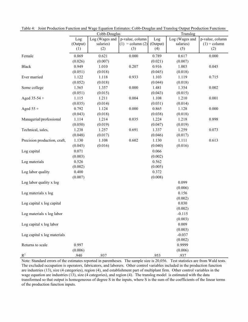
Table 4: Joint Production Function and Wage Equation Estimates: Cobb-Douglas and Translog Output Production FunctionsCobb-Douglas Translog

Log(Output)

(1)

Log (Wages andsalaries)

(2)

p-value, column(1) = column (2)

(3)

Log(Output)

(4)

Log (Wages andsalaries)

(5)

p-value, column(1) = column

(2)

Female 0.869 0.621 0.000 0.789 0.617 0.000(0.026) (0.007) (0.021) (0.007)

Black 0.949 1.010 0.207 0.916 1.003 0.045(0.051) (0.018) (0.045) (0.018)

Ever married 1.122 1.118 0.933 1.103 1.119 0.715(0.052) (0.018) (0.044) (0.018)

Some college 1.565 1.357 0.000 1.481 1.354 0.002(0.051) (0.015) (0.043) (0.015)

Aged 35-54 + 1.115 1.211 0.004 1.108 1.210 0.001(0.035) (0.014) (0.031) (0.014)

Aged 55 + 0.792 1.124 0.000 0.865 1.128 0.000(0.043) (0.018) (0.038) (0.018)

Managerial/professional 1.114 1.214 0.035 1.224 1.218 0.898(0.050) (0.019) (0.047) (0.019)

Technical, sales, 1.238 1.257 0.691 1.337 1.259 0.073(0.048) (0.017) (0.046) (0.017)

Precision production, craft, 1.130 1.108 0.602 1.130 1.111 0.613(0.045) (0.016) (0.040) (0.016)

Log capital 0.071 0.066(0.003) (0.002)

Log materials 0.526 0.562(0.002) (0.005)

Log labor quality 0.400 0.372(0.007) (0.008)

Log labor quality x log 0.099(0.006)

Log materials x log 0.156(0.002)

Log capital x log capital 0.030(0.002)

Log materials x log labor -0.115(0.003)

Log capital x log labor 0.009(0.003)

Log capital x log materials -0.037(0.002)

Returns to scale 0.997 0.9999(0.006) (0.006)

R2 .940 .937 .953 .937Note: Standard errors of the estimates reported in parentheses. The sample size is 20,056. Test statistics are from Wald tests. The excluded occupation is operators, fabricators, and laborers. Other control variables included in the production functionare industries (13), size (4 categories), region (4), and establishment part of multiplant firm. Other control variables in thewage equation are industries (13), size (4 categories), and region (4). The translog model is estimated with the datatransformed so that output is homogeneous of degree S in the inputs, where S is the sum of the coefficients of the linear termsof the production function inputs.

Table 5: Joint Production Function and Wage Equation Estimates: Translog Output Production Functions from DEED andWECD

Translog from DEED Translog from WECD

Log(Output)

(1)

Log(WagesandSalaries)(2)

p-Value,Column 1 =Column 2

(3)

Log(Output)

(4)

Log(WagesandSalaries)(5)

p-Value,Column 1 =Column 2

(6)

Female 0.789 0.617 0.000 0.840 0.549 0.000(0.021) (0.007) (0.064) (0.016)

Black 0.916 1.003 0.045 1.184 1.119 0.628(0.045) (0.018) (0.140) (0.047)

Ever married 1.103 1.119 0.715 1.453 1.371 0.676(0.044) (0.018) (0.207) (0.066)

Some college 1.481 1.354 0.002 1.673 1.432 0.108(0.043) (0.015) (0.156) (0.044)

Aged 35-54 + 1.108 1.210 0.001 1.153 1.193 0.706(0.031) (0.014) (0.108) (0.037)

Aged 55 + 0.865 1.128 0.000 1.192 1.183 0.949(0.038) (0.018) (0.145) (0.051)

Managerial/professional 1.224 1.218 0.898 1.134 0.998 0.294(0.047) (0.019) (0.136) (0.043)

Technical, sales, administrative, and service 1.337 1.259 0.073 1.265 1.111 0.192(0.046) (0.017) (0.124) (0.039)

Precision production, craft, and service 1.130 1.111 0.613 1.060 1.023 0.750(0.040) (0.016) (0.121) (0.039)

Log capital 0.066 0.052(0.002) (0.007)

Log materials 0.562 0.592(0.005) (0.018)

Log labor quality 0.372 0.343(0.008) (0.024)

Log labor quality x log labor quality 0.099 0.106(0.006) (0.016)

Log materials x log materials 0.156 0.153(0.002) (0.007)

Log capital x log capital 0.030 0.021(0.002) (0.008)

Log materials x log labor quality -0.115 -0.123(0.003) (0.007)

Log capital x log labor quality 0.009 0.014(0.003) (0.009)

Log capital x log materials -0.037 -0.027(0.002) (0.006)

Note: Standard errors of the estimates reported in parentheses. The sample size for the DEED sample is 20,056. The samplesize for the WECD is 3,102 and the results in columns (4)-(6) are replicated directly from Hellerstein et al., 1999. Teststatistics are from Wald tests. The excluded occupation is operators, fabricators, and laborers. Other control variablesincluded in the production function are industries (13), size (4 categories), region (4), and establishment part of multiplantfirm. Other control variables in the wage equation are industries (13), size (4 categories), and region (4). The models isestimated with the data transformed so that output is homogeneous of degree S in the inputs, where S is the sum of thecoefficients of the linear terms of the production function inputs.

Table 6: Joint Production Function and Wage Equation Estimates: Cobb-Douglas Production Function, Parsimonious Variantsof the Definition of Labor Quality

Homogeneouslabor(1)

Production/non-production

(2)Four

occupations(3)

High and loweducation

(4)

High and loweducation;production

non-production(5)

High and loweducation; four

occupations(6)

Log (capital) 0.068 0.068 0.068 0.067 0.068 0.067(0.003) (0.003) (0.003) (0.003) (0.003) (0.003)

Log (materials) 0.525 0.525 0.525 0.525 0.525 0.525(0.002) (0.002) (0.002) (0.002) (0.002) (0.002)

Log (labor quality) 0.407 0.406 0.407 0.406 0.406 0.406(0.007) (0.007) (0.007) (0.007) (0.007) (0.007)

Non-Production 1.378 1.081(0.034) (0.032)

Managerial/ professional 1.545 1.095(0.055) (0.048)

Technical, sales, administrative, 1.431 1.188 and service (0.053) (0.046)Precision production, craft, 1.270 1.172 and repair (0.051) (0.045)Some college 1.688 1.619 1.611

(0.045) (0.050) (0.051)R-squared 0.938 0.939 0.939 0.940 0.940 0.940Note: Standard errors in parentheses. The sample size is 20,056. The production function is jointly estimated with the wageequation as in Table 4, columns (1) and (2). The wage equation results are not reported here.

Table 7: Joint Production Function and Wage Equation Estimates: Cobb-Douglas and “Olley-Pakes” ProductionFunctions

Cobb-Douglas Olley-Pakes

Log(Output)

(1)

Log(Wagesandsalaries)(2)

p-Value,Column 1 =Column 2

(3)

Log(Output)

(4)

Log(Wagesandsalaries)(5)

p-Value,Column (1)= Column(2)

Female 0.869 0.621 0.000 0.886 0.623 0.000(0.026) (0.007) (0.028) (0.007)

Black 0.949 1.010 0.207 0.963 1.010 0.351(0.051) (0.018) (0.054) (0.018)

Ever married 1.122 1.118 0.933 1.130 1.119 0.832(0.052) (0.018) (0.055) (0.018)

Some college 1.565 1.357 0.000 1.594 1.358 0.000(0.051) (0.015) (0.055) (0.015)

Aged 35-54 + 1.115 1.211 0.004 1.115 1.211 0.006(0.035) (0.014) (0.037) (0.014)

Aged 55 + 0.792 1.124 0.000 0.795 1.123 0.000(0.043) (0.018) (0.045) (0.018)

Managerial/professional 1.114 1.214 0.035 1.188 1.213 0.642(0.050) (0.019) (0.056) (0.019)

Technical, sales, administrative, and service 1.238 1.257 0.691 1.330 1.256 0.149(0.048) (0.017) (0.054) (0.017)

Precision production, craft, and service 1.130 1.108 0.602 1.108 1.108 0.974(0.045) (0.016) (0.048) (0.016)

Log labor quality 0.400 0.349(0.007) (0.007)

Note: Standard errors of the estimates reported in parentheses. The sample size is 20,056. Test statistics are fromWald tests. The excluded occupation is operators, fabricators, and laborers. Other variables included in the productionfunction for both specifications are log capital, log materials, industries (13), size (4 categories), region (4), andestablishment part of multiplant firm. In the “Olley-Pakes” specification, second and third order terms in log materialsand log capital are also included. Other control variables in the wage equation are industries (13), size (4 categories),and region (4).

Appendix A: Two-Way Frequency of Hand-Checked Scores for All Hand-Checked Data from 1990 DEEDAll Industries

Score BScore A 1 2 3 4 5 Row total

1 9,93066.16

2,22914.85

2911.94

560.37

790.53

12,58583.85

2 1,1267.50

4062.71

950.63

300.20

1,65711.04

3 1581.05

1230.82

2521.68

5333.55

4 400.27

1010.67

1410.94

5 930.62

930.62

Column total 9,93066.16

3,35522.35

8555.70

3142.09

5553.70

15,009100

ManufacturingScore B

Score A 1 2 3 4 5 Row total1 1,981

72.40426

15.5717

0.623

0.110

0.002,427 88.71

2 00

431.57

4 0.15

0 0.00

290 10.60

3 80.29

9 0.33

0 0.00

17 0.62

4 1 0.04

1 0.04

2 0.07

5 0 0.00

0 0.62

Column total 1,98172.40

66924.45

68 2.49

17 0.62

1 0.04

2,736100

Note: Percent of sample in cell is reported in italics in the second entry of each box. We have recorded all non-matching scoresabove the diagonal.