Natural Language Processing (NLP) Applications of …bengioy/ift6266/H13/nlp.pdfNatural Language...
40
Natural Language Processing (NLP) Applications of Deep Learning 1 (taken from IPAM / CIFAR 2012 summer school on deep learning, with parts coming from ACL’2012 tutorial on Deep Learning for NLP, with Richard Socher and Chris Manning) Yoshua Bengio IFT6266 lecture
Transcript of Natural Language Processing (NLP) Applications of …bengioy/ift6266/H13/nlp.pdfNatural Language...

Natural Language Processing (NLP) Applications of Deep Learning
1
(taken from IPAM / CIFAR 2012 summer school on deep learning, with parts coming from ACL’2012 tutorial on Deep Learning for NLP, with Richard Socher and Chris Manning)
Yoshua Bengio IFT6266 lecture
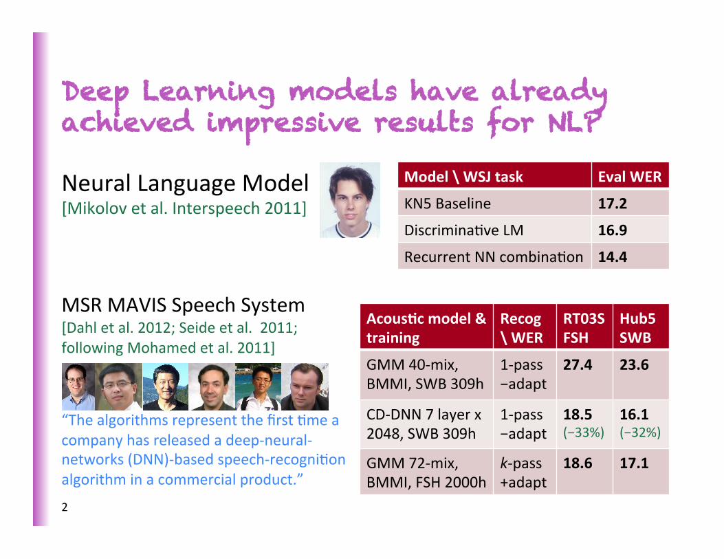
Deep Learning models have already achieved impressive results for NLP
Neural Language Model [Mikolov et al. Interspeech 2011]
MSR MAVIS Speech System [Dahl et al. 2012; Seide et al. 2011; following Mohamed et al. 2011]
“The algorithms represent the first Sme a company has released a deep-‐neural-‐networks (DNN)-‐based speech-‐recogniSon algorithm in a commercial product.”
Model \ WSJ task Eval WER
KN5 Baseline 17.2
DiscriminaSve LM 16.9
Recurrent NN combinaSon 14.4
AcousBc model & training
Recog \ WER
RT03S FSH
Hub5 SWB
GMM 40-‐mix, BMMI, SWB 309h
1-‐pass −adapt
27.4 23.6
CD-‐DNN 7 layer x 2048, SWB 309h
1-‐pass −adapt
18.5 (−33%)
16.1 (−32%)
GMM 72-‐mix, BMMI, FSH 2000h
k-‐pass +adapt
18.6 17.1
2
Existing NLP Applications
• Language Modeling (Speech RecogniSon, Machine TranslaSon) • AcousSc Modeling • Part-‐Of-‐Speech Tagging • Chunking • Named EnSty RecogniSon • SemanSc Role Labeling • Parsing • SenSment Analysis • Paraphrasing • QuesSon-‐Answering • Word-‐Sense DisambiguaSon
3
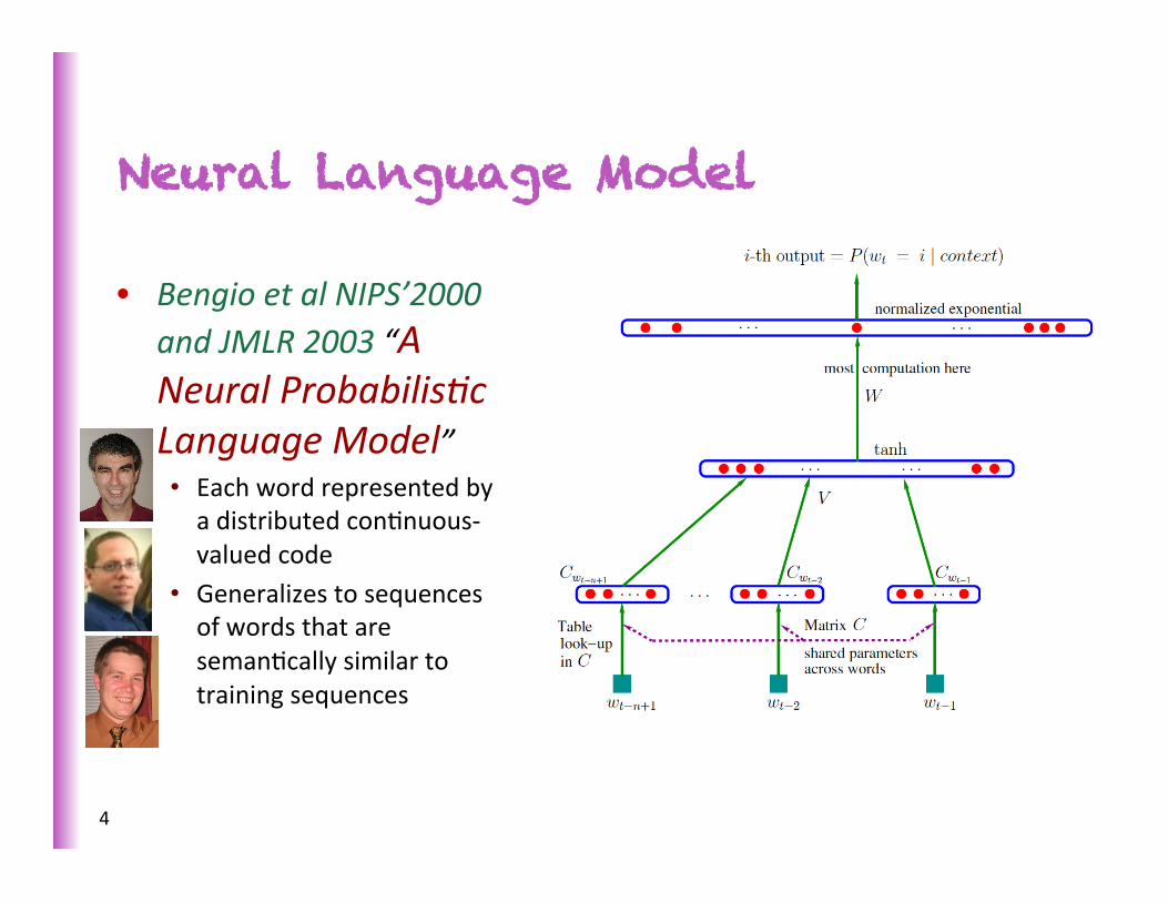
Neural Language Model
• Bengio et al NIPS’2000 and JMLR 2003 “A Neural Probabilis?c Language Model” • Each word represented by a distributed conSnuous-‐valued code
• Generalizes to sequences of words that are semanScally similar to training sequences
4

Language Modeling
• Predict P(next word | previous word)
• Gives a probability for a longer sequence
• ApplicaSons to Speech, TranslaSon and Compression
• ComputaSonal bolleneck: large vocabulary V means that compuSng the output costs #hidden units x |V|.
5

The standard word representation
The vast majority of rule-‐based and staSsScal NLP work regards words as atomic symbols: hotel, conference, walk
In vector space terms, this is a vector with one 1 and a lot of zeroes
[0 0 0 0 0 0 0 0 0 0 1 0 0 0 0] Dimensionality: 20K (speech) – 50K (PTB) – 500K (big vocab) – 13M (Google 1T)
We call this a “one-‐hot” representaSon. Its problem:
motel [0 0 0 0 0 0 0 0 0 0 1 0 0 0 0] AND hotel [0 0 0 0 0 0 0 1 0 0 0 0 0 0 0] = 0
6

Distributional similarity based representations
You can get a lot of value by represenSng a word by means of its neighbors
“You shall know a word by the company it keeps” (J. R. Firth 1957: 11)
One of the most successful ideas of modern staSsScal NLP government debt problems turning into banking crises as has happened in
saying that Europe needs unified banking regulation to replace the hodgepodge
ë These words will represent banking ì
7
You can vary whether you use local or large context to get a more syntacSc or semanSc clustering
Class-based (hard) and soft clustering word representations
Class based models learn word classes of similar words based on distribuSonal informaSon ( ~ class HMM) • Brown clustering (Brown et al. 1992) • Exchange clustering (MarSn et al. 1998, Clark 2003) • DesparsificaSon and great example of unsupervised pre-‐training
Sot clustering models learn for each cluster/topic a distribuSon over words of how likely that word is in each cluster • Latent SemanSc Analysis (LSA/LSI), Random projecSons • Latent Dirichlet Analysis (LDA), HMM clustering 8
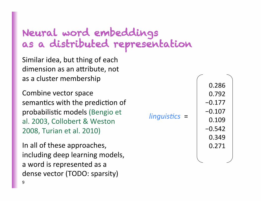
Neural word embeddings as a distributed representation Similar idea, but thing of each dimension as an alribute, not as a cluster membership
Combine vector space semanScs with the predicSon of probabilisSc models (Bengio et al. 2003, Collobert & Weston 2008, Turian et al. 2010)
In all of these approaches, including deep learning models, a word is represented as a dense vector (TODO: sparsity)
linguis?cs =
9
0.286 0.792 −0.177 −0.107 0.109 −0.542 0.349 0.271

Neural word embeddings - visualization
10
Advantages of the neural word embedding approach
11
Compared to a method like LSA, neural word embeddings can become more meaningful through adding supervision from one or mulSple tasks
For instance, senSment is usually not captured in unsupervised word embeddings but can be in neural word vectors
We can build representaSons for large linguisSc units
See below
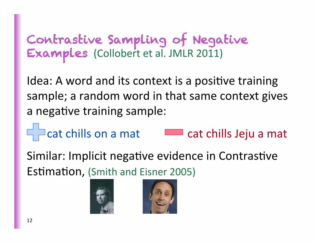
Contrastive Sampling of Negative Examples (Collobert et al. JMLR 2011)
Idea: A word and its context is a posiSve training sample; a random word in that same context gives a negaSve training sample:
cat chills on a mat cat chills Jeju a mat
Similar: Implicit negaSve evidence in ContrasSve EsSmaSon, (Smith and Eisner 2005)
12
A neural network for learning word vectors
13
How do we formalize this idea? Ask that score(cat chills on a mat) > score(cat chills Jeju a mat)
How do we compute the score?
• With a neural network • Each word is associated with an
n-‐dimensional vector

Word embedding matrix
• IniSalize all word vectors randomly to form a word embedding matrix |V|
L = … n
the cat mat … • These are the word features we want to learn • Also called a look-‐up table
• Conceptually you get a word’s vector by let mulSplying a one-‐hot vector e by L: x = Le
[ ]
14
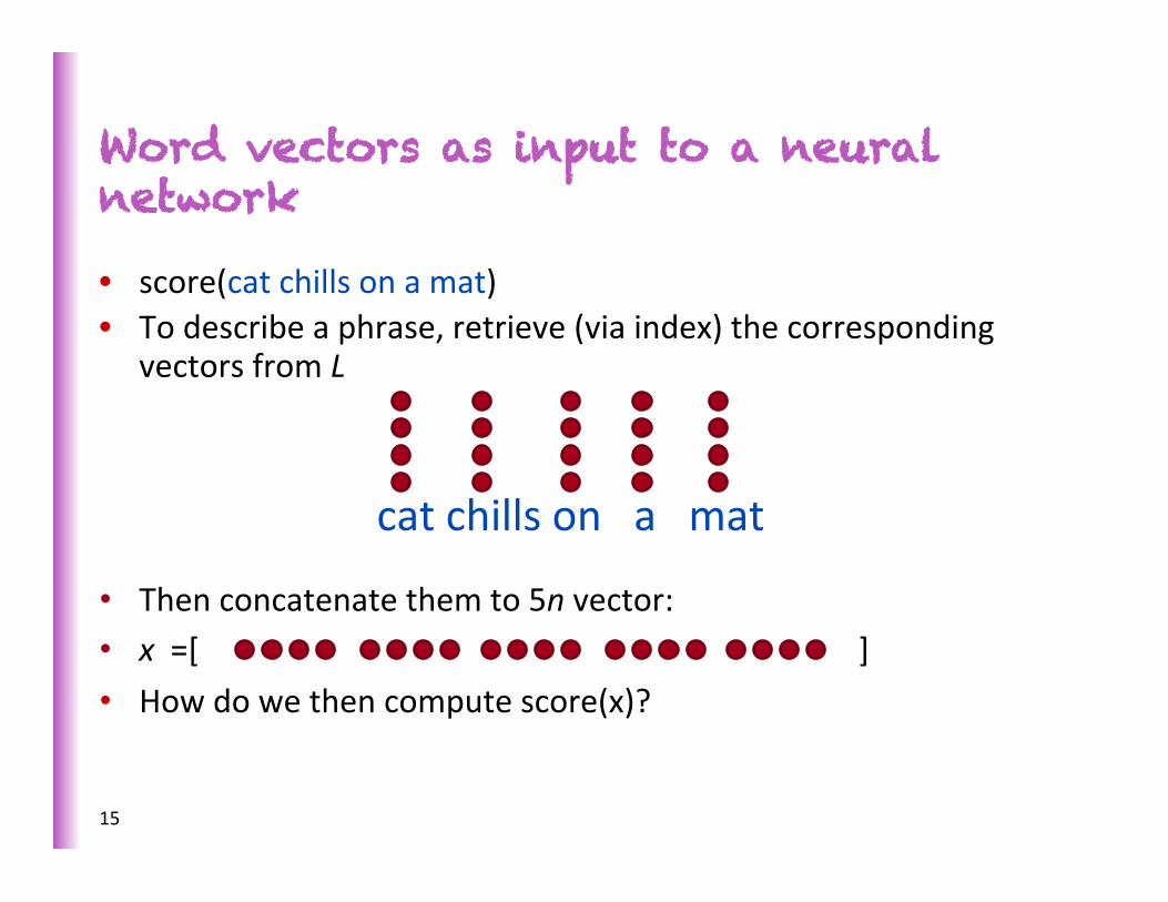
• score(cat chills on a mat) • To describe a phrase, retrieve (via index) the corresponding
vectors from L
cat chills on a mat
• Then concatenate them to 5n vector: • x =[ ] • How do we then compute score(x)?
Word vectors as input to a neural network
15

POS WSJ (acc.)
NER CoNLL (F1)
State-‐of-‐the-‐art* 97.24 89.31 Supervised NN 96.37 81.47 Unsupervised pre-‐training followed by supervised NN**
97.20 88.87
+ hand-‐crated features*** 97.29 89.59 * RepresentaSve systems: POS: (Toutanova et al. 2003), NER: (Ando & Zhang 2005) ** 130,000-‐word embedding trained on Wikipedia and Reuters with 11 word window, 100 unit hidden layer – for 7 weeks! – then supervised task training ***Features are character suffixes for POS and a gazeleer for NER
The secret sauce is the unsupervised pre-training on a large text collection
16
(Collobert & Weston 2008; Collobert et al. 2011)

POS WSJ (acc.)
NER CoNLL (F1)
Supervised NN 96.37 81.47 NN with Brown clusters 96.92 87.15 Fixed embeddings* 97.10 88.87 C&W 2011** 97.29 89.59
* Same architecture as C&W 2011, but word embeddings are kept constant during the supervised training phase ** C&W is unsupervised pre-‐train + supervised NN + features model of last slide
Supervised refinement of the unsupervised word representation helps
17

Bilinear Language Model
• Even a linear version of the Neural Language Model works
beler than n-‐grams
r̂ =X
i
Cirwir̂
C
rwi
|V|-length Softmax layer
n-length Embedding layer
• [Mnih & Hinton 2007] • APNews perplexity
down from 117 (KN6) to 96.5
18
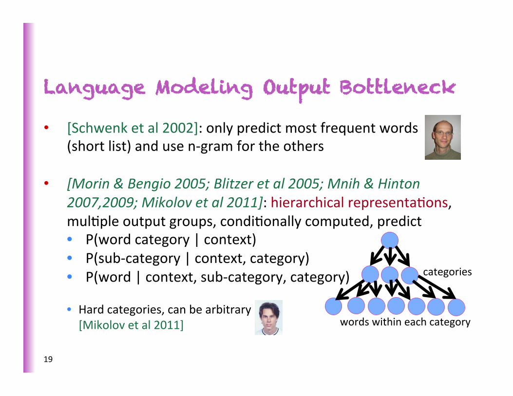
Language Modeling Output Bottleneck
• [Schwenk et al 2002]: only predict most frequent words (short list) and use n-‐gram for the others
• [Morin & Bengio 2005; Blitzer et al 2005; Mnih & Hinton 2007,2009; Mikolov et al 2011]: hierarchical representaSons, mulSple output groups, condiSonally computed, predict • P(word category | context) • P(sub-‐category | context, category) • P(word | context, sub-‐category, category)
• Hard categories, can be arbitrary [Mikolov et al 2011]
categories
words within each category
19

Language Modeling Output Bottleneck: Hierarchical word categories
Compute
P(word|category,context) only for category=category(word)
P(category|context)
InstanSated only for category(word)
…
… Context = previous words
P(word|context,category)
20

Language Modeling Output Bottleneck: Sampling Methods
• Importance sampling to recover next-‐word probabiliSes [Bengio & Senecal 2003, 2008]
• ContrasSve Sampling of negaSve examples, with a ranking loss [Collobert et al, 2008, 2011]
• (no probabiliSes, ok if the goal is just to learn word embeddings)
• Importance sampling for reconstrucSng bag-‐of-‐words [Dauphin
et al 2011]
21
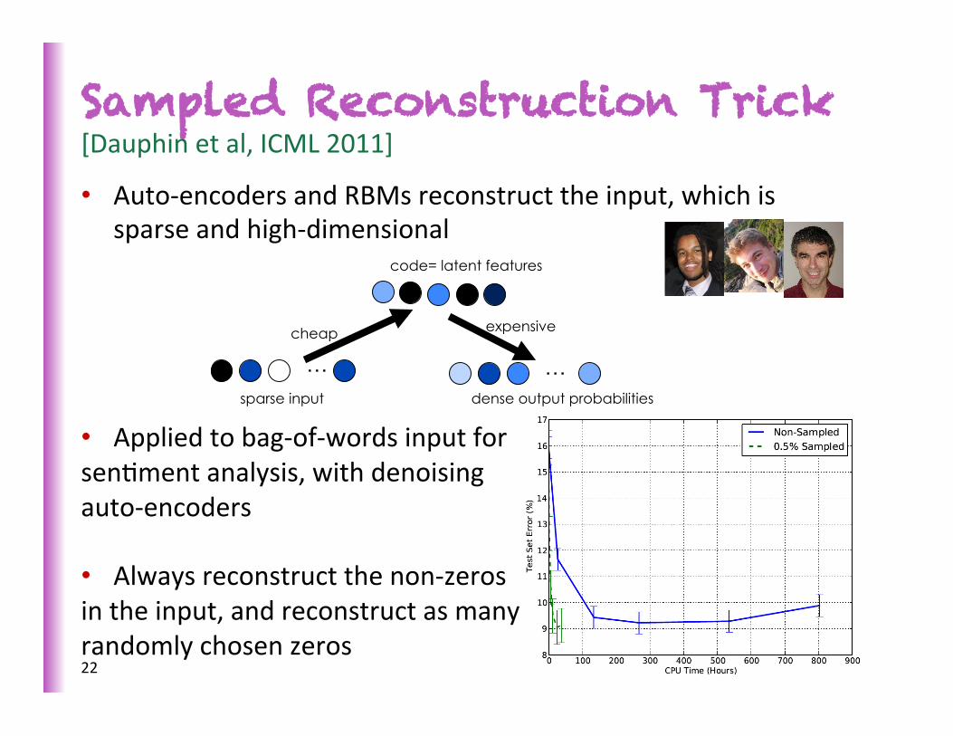
Sampled Reconstruction Trick [Dauphin et al, ICML 2011]
• Auto-‐encoders and RBMs reconstruct the input, which is sparse and high-‐dimensional
• Applied to bag-‐of-‐words input for senSment analysis, with denoising auto-‐encoders
• Always reconstruct the non-‐zeros in the input, and reconstruct as many randomly chosen zeros
…
code= latent features
… sparse input dense output probabilities
cheap expensive
22
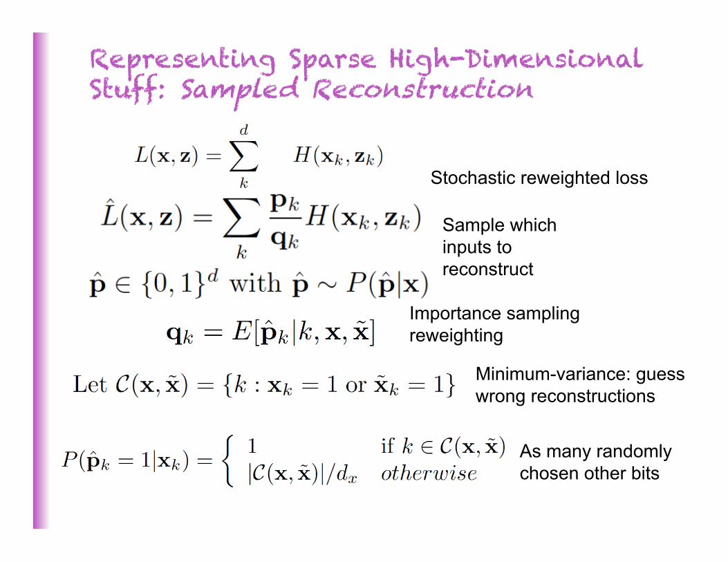
Representing Sparse High-Dimensional Stuff: Sampled Reconstruction
Sample which inputs to reconstruct
Importance sampling reweighting
Minimum-variance: guess wrong reconstructions
As many randomly chosen other bits
Stochastic reweighted loss

Recurrent Neural Net Language Modeling for ASR
• [Mikolov et al 2011] Bigger is beler… experiments on Broadcast News NIST-‐RT04
perplexity goes from 140 to 102
Paper shows how to train a recurrent neural net with a single core in a few days, with > 1% absolute improvement in WER
Code: http://www.fit.vutbr.cz/~imikolov/rnnlm/!
Code: hlp://www.fit.vutbr.cz/~imikolov/rnnlm/
24
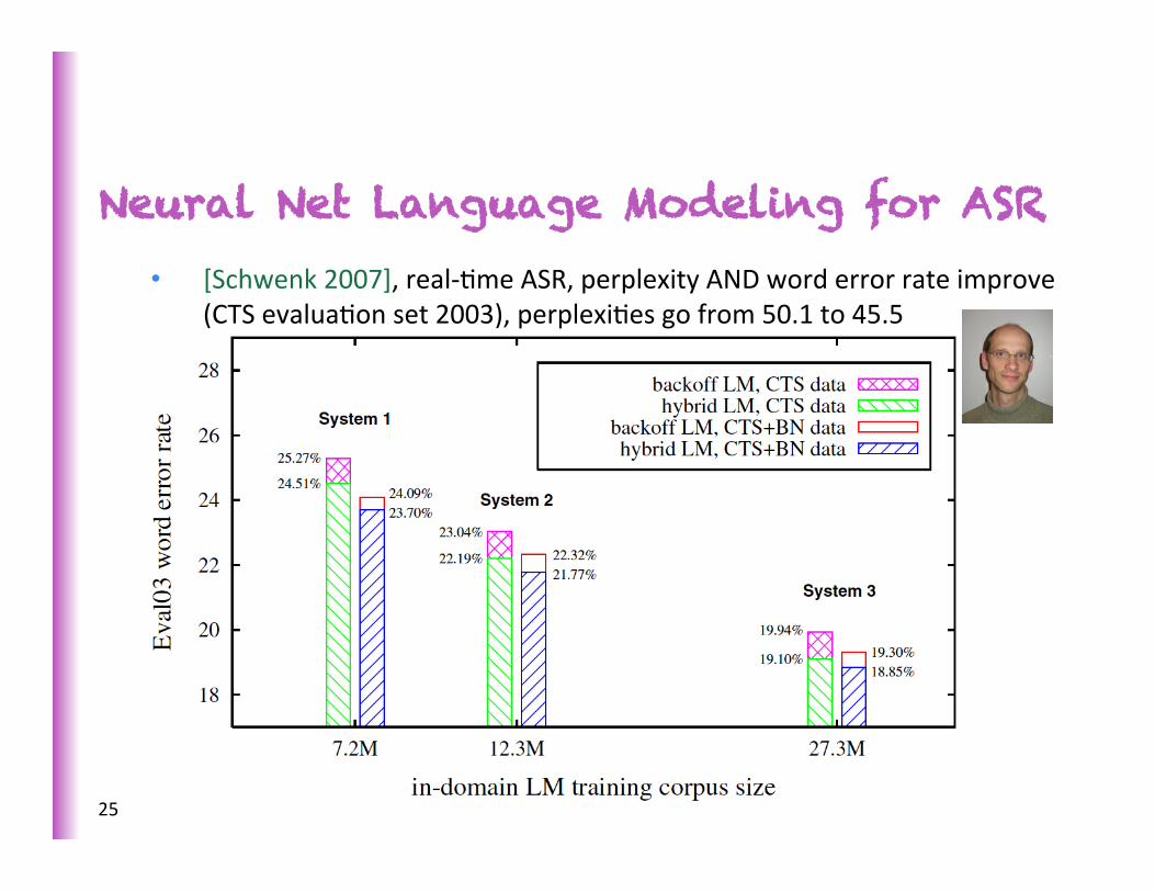
Neural Net Language Modeling for ASR
• [Schwenk 2007], real-‐Sme ASR, perplexity AND word error rate improve (CTS evaluaSon set 2003), perplexiSes go from 50.1 to 45.5
25

Application to Statistical Machine Translation
• Schwenk (NAACL 2012 workshop on the future of LM) • 41M words, Arabic/English bitexts + 151M English from LDC
• Perplexity down from 71.1 (6 Gig back-‐off) to 56.9 (neural model, 500M memory)
• +1.8 BLEU score (50.75 to 52.28)
• Can take advantage of longer contexts
• Code: http://lium.univ-lemans.fr/cslm/!
26

Learning Structured Embeddings of Knowledge Bases, (Bordes, Weston, Collobert & Bengio, AAAI 2011) Joint Learning of Words and Meaning Representa?ons for Open-‐Text Seman?c Parsing, (Bordes, Glorot, Weston & Bengio, AISTATS 2012)
Modeling Semantics
27

Model (lhs, relaSon, rhs) Each concept = 1 embedding vector Each relaSon = 2 matrices. Matrix or mlp acts as operator. Ranking criterion Energy = low for training examples, high o/w
lhs relaSon
energy
rhs
choose vector
choose matrices
|| . ||1
Modeling Relations: Operating on Embeddings
28
Subj. words Verb words
energy
Obj. words
|| . ||1
mlp mlp
Element-‐wise max. Element-‐wise max. Element-‐wise max.
black__2 eat__2 cat__1 white__1 mouse_2

Verb = relaSon. Too many to have a matrix each. Each concept = 1 embedding vector Each relaSon = 1 embedding vector Can handle relaSons on relaSons on relaSons
Allowing Relations on Relations
lhs relaSon
energy
rhs
choose vector
|| . ||1
mlp mlp
29
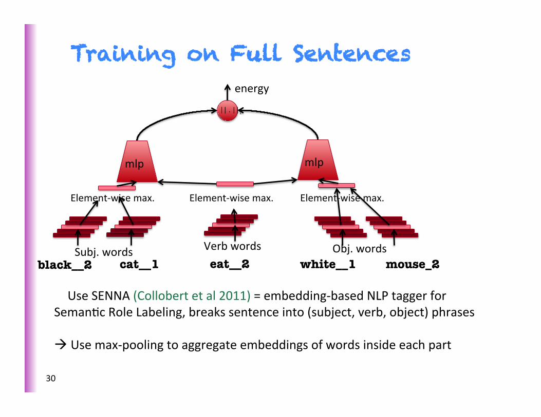
Training on Full Sentences
Subj. words Verb words
energy
Obj. words
|| . ||1
mlp mlp
Element-‐wise max. Element-‐wise max. Element-‐wise max.
black__2 eat__2 cat__1 white__1 mouse_2
à Use SENNA (Collobert et al 2011) = embedding-‐based NLP tagger for SemanSc Role Labeling, breaks sentence into (subject, verb, object) phrases
à Use max-‐pooling to aggregate embeddings of words inside each part
30

Open-Text Semantic Parsing
• 3 steps:
• last formula defines the Meaning RepresentaSon (MR).
31

Training Criterion
• IntuiSon: if an enSty of a triplet was missing, we would like our model to predict it correctly i.e. to give it the lowest energy. For example, this would allow us to answer quesSons like “what is part of a car?”
• Hence, for any training triplet xi = (lhsi, reli, rhsi) we would like: (1) E(lhsi, reli, rhsi) < E(lhsj, reli, rhsi), (2) E(lhsi, reli, rhsi) < E(lhsi, relj, rhsi), (3) E(lhsi, reli, rhsi) < E(lhsi, reli, rhsj),
That is, the energy funcSon E is trained to rank training samples below all other triplets.
32

Contrastive Sampling of Neg. Ex.= pseudo-likelihood + uniform sampling of negative variants
Train by stochasSc gradient descent: 1. Randomly select a posiSve training triplet xi = (lhsi, reli, rhsi). 2. Randomly select constraint (1), (2) or (3) and an enSty ẽ: -‐ If constraint (1), construct negaSve triplet x ̃ = (ẽ, reli, rhsi). -‐ Else if constraint (2), construct x ̃ = (lhsi, ẽ, rhsi). -‐ Else, construct x ̃ = (lhsi, reli, ẽ). 3. If E(xi) > E(x ̃) − 1 make a gradient step to minimize:
max(0, 1 − E(x ̃) + E(xi)). 4. Constraint embedding vectors to norm 1
33
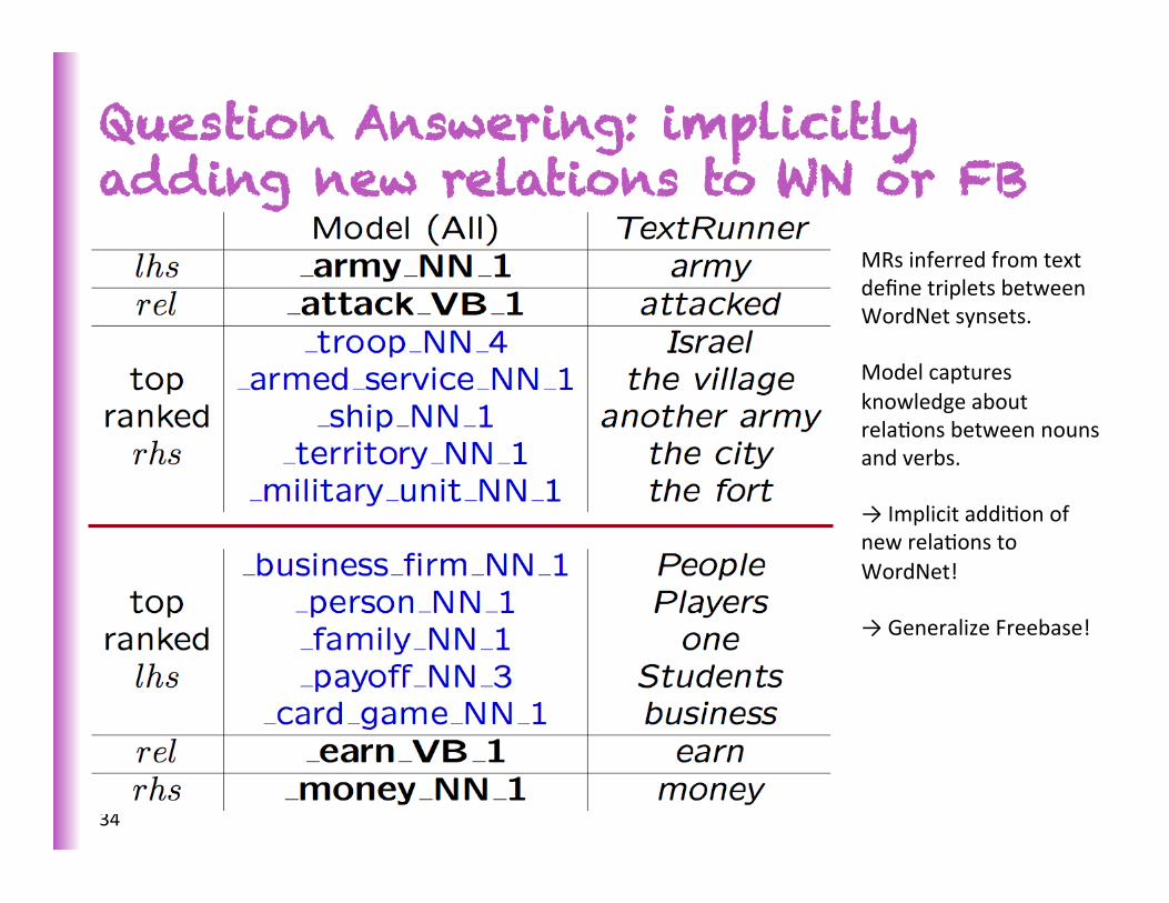
Question Answering: implicitly adding new relations to WN or FB
34
MRs inferred from text define triplets between WordNet synsets. Model captures knowledge about relaSons between nouns and verbs. → Implicit addiSon of new relaSons to WordNet! → Generalize Freebase!
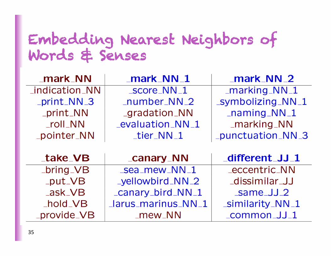
Embedding Nearest Neighbors of Words & Senses
35

Word Sense Disambiguation • Senseval-‐3 results
(only sentences with Subject-‐Verb-‐Object structure)
MFS=most frequent sense All=training from all sources Gamble=Decadt et al 2004 (Senseval-‐3 SOA)
• XWN results XWN = eXtended WN
36

Learning Multiple Word Vectors
• Tackles problems with polysemous words
• Can be done with both standard �-‐idf based methods [Reisinger and Mooney, NAACL 2010]
• Recent neural word vector model by [Huang et al. ACL 2012] learns mulSple prototypes using both local and global context
• State of the art correlaSons with human similarity judgments
37
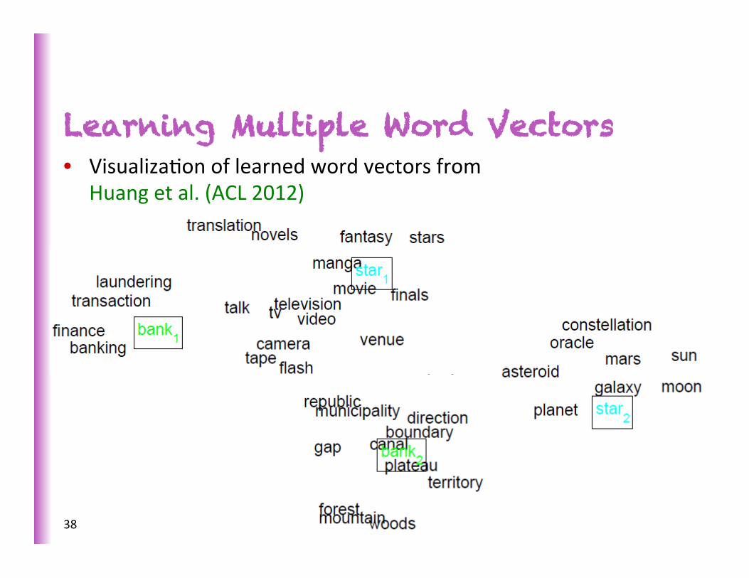
Learning Multiple Word Vectors • VisualizaSon of learned word vectors from
Huang et al. (ACL 2012)
38
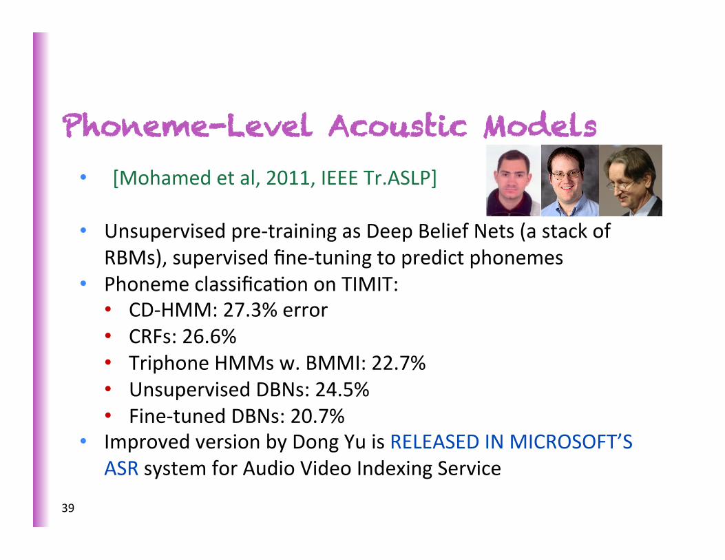
Phoneme-Level Acoustic Models
• [Mohamed et al, 2011, IEEE Tr.ASLP]
• Unsupervised pre-‐training as Deep Belief Nets (a stack of RBMs), supervised fine-‐tuning to predict phonemes
• Phoneme classificaSon on TIMIT: • CD-‐HMM: 27.3% error • CRFs: 26.6% • Triphone HMMs w. BMMI: 22.7% • Unsupervised DBNs: 24.5% • Fine-‐tuned DBNs: 20.7%
• Improved version by Dong Yu is RELEASED IN MICROSOFT’S ASR system for Audio Video Indexing Service
39
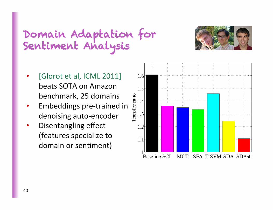
Domain Adaptation for Sentiment Analysis
• [Glorot et al, ICML 2011] beats SOTA on Amazon benchmark, 25 domains
• Embeddings pre-‐trained in denoising auto-‐encoder
• Disentangling effect (features specialize to domain or senSment)
40