NATIONAL TECHNICAL UNIVERSITY OF ATHENS · Aristoteles Tegos Athens, 2019 . NATIONAL TECHNICAL...
123
NATIONAL TECHNICAL UNIVERSITY OF ATHENS SCHOOL OF CIVIL ENGINEERING DEPARTMENT OF WATER RESOURCES AND ENVIRONMENTAL ENGINEERING State-of-the-art approach for potential evapotranspiration assessment Ph.D Thesis Aristoteles Tegos Athens, 2019
Transcript of NATIONAL TECHNICAL UNIVERSITY OF ATHENS · Aristoteles Tegos Athens, 2019 . NATIONAL TECHNICAL...

NATIONAL TECHNICAL UNIVERSITY OF ATHENS
SCHOOL OF CIVIL ENGINEERING
DEPARTMENT OF WATER RESOURCES AND ENVIRONMENTAL ENGINEERING
State-of-the-art approach for potential evapotranspiration
assessment
Ph.D Thesis
Aristoteles Tegos
Athens, 2019


NATIONAL TECHNICAL UNIVERSITY OF ATHENS
SCHOOL OF CIVIL ENGINEERING
DEPARTMENT OF WATER RESOURCES AND ENVIRONMENTAL ENGINEERING
State-of-the-art approach for potential evapotranspiration
assessment
Thesis submitted for the degree of Doctor of Engineering at the
National Technical University of Athens
Aristoteles Tegos
Athens, 2019

THESIS COMMITEE
THESIS SUPERVISOR
Demetris Koutsoyiannis, Professor, N.T.U.A
ADVISORY COMMITTEE
1. Demetris Koutsoyiannis, Professor, N.T.U.A (Supervisor)
2. Nikos Mamassis- Associate Professor, N.T.U.A
3. Dr. Konstantine Georgakakos, Sc.D Hydrologic Research Center in San Diego,
California- Adjunct Professor, Scripps Institution of Oceanography, University of
California San Diego
EVALUATION COMMITTEE
1. Demetris Koutsoyiannis, Professor, N.T.U.A (Supervisor)
2. Nikos Mamassis, Associate Professor, N.T.U.A
3. Dr. Konstantine Georgakakos, Sc.D Hydrologic Research Center in San Diego,
California- Adjunct Professor, Scripps Institution of Oceanography, University of
California San Diego
4. Evanglelos Baltas, Professor, N.T.U.A
5. Athanasios Loukas, Associate Professor, A.U.Th
6. Stavros Alexandris, Associate Professor, Agricultural University of Athens
7. Nikolaos Malamos, Assistant Professor, University of Patras

Κάποτε υπό άλλη φυσική συνθήκη
και κάτω από άλλη φυσική κατάσταση
Θα συζητήσουμε τις ιδέες μας και θα γελάμε.
Προς το παρόν για σένα Πατέρα


Abstract
The aim of the Ph.D thesis is the foundation of a new temperature-based model since simplified
PET estimation proves very useful in absence of a complete data set. In this respect, the Parametric
model is presented based on a simplified formulation of the well-established Penman-Monteith
expression, which only requires mean daily or monthly temperature data. The model was applied at
both global and local regions and the outcomes of this new approach are very encouraging, as
indicated by the substantially high validation scores of the proposed approach across all examined
data sets. In general, the parametric model outperforms well-established methods of the everyday
practice. A second analysis which was examined as part of this thesis is related to which spatial
techniques is the optimal in order to transform the point scale estimate in regional. A thorough
analysis of different geostatistical model was carried out (Kriging, IDW, NN, BSS) and it can be
concluded that the IDW even is the most simplify geostatistical model, it can be produce consistent
spatial PET results.
Another part of the thesis was the development of an R function for testing the trend significance of
time series. The function calculates the trend significance using a modified Mann- Kendall test,
which takes into account the well-known physical behavior of the Hurst-Kolmogorov dynamics. The
function is tested in 10 stations in Greece, with approximately 50 years of PET data with the use of a
recent parametric model.
Finally, a number of hydrological, agronomist and climatologist applications are presented for
lighting the robustness of the new Parametric approach in multidiscipline areas.
Keywords: Potential evapotranspiration; Parametric model; Penman- Monteith method; large
scale hydrology, Calibration, Remote Sensing; Spatial analysis; trend; Hurst; R-script; CLIMWAT;
CIMIS

Περίληψη
Ο σκοπός της Διδακτορικής Διατριβής είναι η θεμελίωση μιας νέας σχέσης θερμοκρασίας για την
εκτίμηση της δυνητικής εξατμοδιαπνοής, καθώς τα απλοποιημένα μοντέλα εκτίμησης είναι
εξαιρετικά χρήσιμα σε καθεστώς έλλειψης πρωτογενών δεδομένων. Σε αυτό το πλαίσιο,
παρουσιάζεται το Παραμετρικό Mοντέλο που αποτελεί απλοποίηση του καταξιωμένου μοντέλου
Penman-Monteith και το οποίο απαιτεί τη μέση ημερήσια θερμοκρασία ή τη μέση μηνιαία
θερμοκρασία ως δεδομένο εισόδου. Το μοντέλο εφαρμόστηκε σε παγκόσμιο και σε τοπικό πεδίο
και τα αποτελέσματα είναι πολύ ενθαρρυντικά, καθώς συνοδεύεται από μεγάλη αποδοτικότητα σε
όλα τα πεδία εφαρμογής του. Γενικά, το παραμετρικό μοντέλο υπερισχύει όλων των εδραιωμένων
μοντέλων ακτινοβολίας και διασφαλίζει τη βέλτιστη εκτίμηση της δυνητικής εξατμοδιαπνοής. Ένα
δεύτερο επίπεδο μελέτης της παρούσας διατριβής σχετίζεται με το ποιο μοντέλο γεωστατιστικής
είναι το βέλτιστο για τη μετατροπή της σημειακής πληροφορίας σε χωρική. Πραγματοποιήθηκε
συστηματική μελέτη διαφορετικών τεχνικών γεωγραφικής ολοκλήρωσης και το αποτέλεσμα είναι
ότι η μέθοδος Αντιστρόφου Σταθμισμένης Απόστασης είναι η βέλτιστη παρόλο που είναι η
απλούστερη από όσες εφαρμόστηκαν.
Άλλο κομμάτι της διατριβής ήταν η ανάπτυξη ενός εργαλείου σε περιβάλλον R για την εκτίμηση
των τάσεων σε χρονοσειρές. Η μεθοδολογία εκτιμά τις τάσεις με ένα τροποποιημένο στατιστικό
έλεγχο Mann-Kendall λαμβάνοντας υπόψη τη φυσική συμπεριφορά της δυναμικής Hurst-
Kolmogorov.
Τέλος, μέσω υδρολογικών, γεωπονικών και κλιματολογικών εφαρμογών αξιολογείται η
χρησιμότητα του Παραμετρικού μοντέλου σε διαφορετικά επιστημονικά πεδία.
Keywords: Δυνητική Εξατμοδιαπνοή; Παραμετρικό Μοντέλο; Penman- Monteith μέθοδος;
Υδρολογία Μεγάλης Κλίμακας, Βαθμονόμηση; Τηλεπισκόπηση; Χωρική Ανάλυση; Τάση; Hurst; R-
script; CLIMWAT; CIMIS

Ευχαριστίες
«Κλείνοντας» αυτόν τον πλήρη κύκλο ακαδημαϊκών σπουδών που μάλλον όσον αφορά τη μάθηση
είναι μια πράξη αέναη, νιώθω λίγο κενός για να εκφράσω σε λίγες λέξεις τα αισθήματα μου.
Αναγκαστικά όμως θα αποπειραθώ να το κάνω.
Κατά ένα παράξενο τρόπο και λόγω του ότι είμαι Μηχανικός της πράξης με πιθανά ανύπαρκτη
ακαδημαϊκή προοπτική, μένω με το ερώτημα γιατί ένας από του γνωστότερους Υδρολόγους της
Παγκόσμιας Ιστορίας, ο Ιρλανδός James Clement Dooge, ξεκίνησε την καριέρα του σαν απλός
υδρολόγος-μηχανικός για περίπου 15 χρόνια πριν ολοκληρώσει επιτυχώς τις διδακτορικές
σπουδές και γίνει ένας από τους σημαντικότερους επιστήμονες στο πεδίο της Υδρολογίας. Νομίζω
ότι μόνο αυτό το ερώτημα με κράτησε προσηλωμένο στην ολοκλήρωση της διατριβής και πιθανά
αφορά στην άδολη αγάπη για την εξερεύνηση πρακτικών ιδεών υπό καθεστώς ελευθερίας. Είμαι
βέβαιος ότι το τέλος αυτής της πορείας με βρίσκει χρησιμότερο επιστήμονα και αποδοτικότερο
Μηχανικό της καθημερινότητας.
Το καθεστώς Ελευθερίας το χρωστάω στον επιβλέποντα της διατριβής Δημήτρη Κουτσογιάννη,
Καθηγητή Ε.Μ.Π, που για περίπου 15 χρόνια τριγυρνάω δίπλα του και καθότι είναι λάτρης της
Ρωσικής Επιστήμης είμαι σίγουρος ότι όλοι/ες μας «δεν θα μπορέσουμε ποτέ να του
ξεπληρώσουμε όσα του χρωστάμε». Πολλές ευχαριστίες στο Νίκο Μαμάση, Αναπληρωτή
Καθηγητή Ε.Μ.Π και μέλος της συμβουλευτικής επιτροπής της παρούσας διατριβής για τη βοήθεια
του όλα αυτά τα χρόνια με το δικό του αυθεντικό τρόπο. Τέλος, στο Δρ. Κωνσταντίνο Γεωργακάκο,
Sc. D επίσης μέλος της συμβουλευτικής επιτροπής που ήταν πάντα παρόν στην εξέλιξη της
παρούσας Δ.Δ και σε μία σειρά άλλων επιστημονικών θεμάτων. Ξεχωριστά θέλω να τονίσω την
σημαντικότατη συνεισφορά του Δρ. Ανδρέα Ευστρατιάδη για την επιμονή του να γίνει αυτή η
εργασία και τις άλλες ιδέες που μας ένωσαν και του Δρ. Νικόλα Μαλάμου, Επίκουρου Καθηγητή
και μέλος της Επταμελούς Επιτροπής, του οποίου η συμβολή του σε όλες τις φάσεις της διατριβής
ήταν καθοριστική και νομίζω ότι μοιραστήκαμε μαζί τη χαρά των καλών αποτελεσμάτων της
παρούσας εργασίας. Θερμές ευχαριστίες για τη συνεισφορά και την εποικοδομητική τους κριτική
στα μέλη της Επιτροπής Εξέτασης κ. Δρ. Σταύρο Αλεξανδρή, Αναπληρωτή Καθηγητή Γ.Π.Α, Δρ.
Αθανάσιο Λουκά, Αναπληρωτή Καθηγητή Α.Π.Θ και Ευάγγελο Μπαλτά Καθηγητή Ε.Μ.Π. Ένα
ακόμη ευχαριστώ στον Καθηγητή Ανδρέα Ανδρεαδάκη για την παροχή συστατικής επιστολής για
την εγγραφή μου ως Υ.Δ και σε όλα τα ακαδημαϊκά μέλη του τομέα και της σχολής που
επικύρωσαν την εγγραφή μου. Μπορεί να υπήρξαν σημαντικές διαφωνίες για την καταλληλότητα
μου λόγω “προχωρημένης ηλικίας” και ίσως άλλων λόγων που δεν γνωρίζω αλλά τελικά καταλήγω
σε σχετικά μικρό χρονικό διάστημα να παραδίδω ένα πολυσύνθετο επιστημονικό έργο, όπως
αποδεικνύεται από το πλήθος των υπό κρίση δημοσιεύσεων μου και αναφορών άλλων μέχρι
σήμερα. Οι όποιες διαφωνίες και ενστάσεις καμία σημασία δεν έχουν σήμερα, καθώς «το λέει και
ένα τραγούδι που μας μάθαιναν παλιά, ο χαμένος τα παίρνει όλα».
Θα ήθελα να καταθέσω και γραπτώς την ευγνωμοσύνη μου και την αγάπη μου σε όλα τα μέλη της
ΙΤΙΑΣ για τη φιλία και τη συνεργασία όλα αυτά τα χρόνια. Στον Αντώνη Κουκουβίνο για τα δικά

μας σχέδια, στον Χρήστο Τύραλη για την στρατιωτικά αποδοτική του συνεργασία, στον Δρ.
Παναγιώτη Δημητριάδη που είναι καλός αλλά δεν με ακούει ποτέ, στον Παναγιώτη Κοσσιέρη για
την ομορφιά του και τον Δρ. Ιωάννη Τσουκαλά για την «ευγενική χορηγία της ευφυΐας του». Τέλος
για τη φιλία τους και τη συνεργασία του το Γιάννη Μαρκόνη, το Σίμωνα Παπαλεξίου και το Φοίβο
Σαργέντη.
Η εργασία δεν θα ολοκληρώνονταν αν δεν ζούσα στην Ιρλανδία που η καθολική ευγένεια του
πληθυσμού της ακόμα και στις καθημερινές μετακινήσεις με το τρένο διαμορφώνουν ένα
κατάλληλο περιβάλλον για να δουλέψεις και στις πλέον αντίξοες συνθήκες με την αναγκαία
προσήλωση. Ευχαριστώ λοιπόν ανώνυμε Ιρλανδέ και Ιρλανδέζα! Σε αυτό το σημείο να
ευχαριστήσω και επωνύμως τους Ιρλανδούς συναδέλφους κ.κ. Dr. Connie O'Driscoll, Dr. Maebh
Grace, Dr. Tracey Lydon και Dr. Raymond Brendan για το πρώτο «σκανάρισμα» του διδακτορικού
και τις εποικοδομητικές τους παρατηρήσεις.
Από τον επαγγελματικό χώρο των μηχανικών δεν θα ξεχάσω το Δρ. Παναγιώτη- Διονύσιο
Παναγόπουλο που λόγω της καθημερινής μας τριβής παλιότερα, μου μετέφερε την αγάπη που
πρέπει να έχει ο μηχανικός στην επιστήμη και το νέο. Ακόμη τον νεότερο συνάδερφο Αλέξανδρο
Καρανάσιο που η επίβλεψη της διπλωματικής του εργασίας ήταν σημαντικό στοιχείο της
παρούσας εργασίας.
Τέλος πολλές ευχαριστίες στην κ. Πηνελόπη Τσίρα για την υπομονή της, την περιποίηση και την
αγάπη όλα αυτά τα χρόνια και φυσικά στα παιδιά μας Μαριλένα και Χρήστο που όταν θα έρθει η
ώρα θα αποκωδικοποιήσουν με το δικό τους τρόπο τι προσπάθησε να τους κληροδοτήσει ο
Πατέρας τους.
Ιρλανδία 2019,
Αριστοτέλης Τέγος


Contents
1 Introduction ................................................................................................................................................................... 1
1.1 Overview ...................................................................................................................................................................... 1
1.2 Scientific innovations of the thesis .................................................................................................................... 2
2 Overview of PET models ........................................................................................................................................... 4
2.1 The potential evapotranspiration process ..................................................................................................... 4
2.2 Historical overview of PET modelling .............................................................................................................. 5
2.2.1 General ............................................................................................................................................................... 5
2.2.2 Radiation-based models ............................................................................................................................. 8
2.2.3 The value of the calibrated radiation- based PET models ............................................................ 9
2.2.4 PET impacts in hydrological modelling ............................................................................................... 9
2.2.5 Outstanding issues ...................................................................................................................................... 11
3 Global Parametric model development ............................................................................................................ 12
3.1 Introduction ............................................................................................................................................................. 12
3.1.1 Theoretical Background ........................................................................................................................... 14
3.1.2 The Parametric Formula .......................................................................................................................... 15
3.1.3 Modified Parametric Model .................................................................................................................... 16
3.1.4 The CLIMWAT Database: Preliminary Analysis ............................................................................. 16
3.1.5 Conclusions .................................................................................................................................................... 37
4 Parametric model in CIMIS network .................................................................................................................. 39
4.1 Introduction ............................................................................................................................................................. 39
4.2 Parametric formula ............................................................................................................................................... 39
4.3 Radiation-Based and temperature-based models .................................................................................... 40
4.4 Hydrometeorological data and computational tools .............................................................................. 41
4.5 Statistical criteria ................................................................................................................................................... 42
4.6 Results ........................................................................................................................................................................ 43
4.7 Comparison with radiation-based methods ............................................................................................... 44
4.8 Comparison with temperature-based methods ........................................................................................ 47
4.9 Spatial analysis of the parameters .................................................................................................................. 48
4.10 Correlation to latitude and elevation ............................................................................................................ 48

4.11 Spatial interpolation over California ............................................................................................................. 49
4.12 Discussions and Conclusions ............................................................................................................................ 54
5 Global PET maps based on monthly remote temperatures ...................................................................... 56
5.1 Introduction ............................................................................................................................................................. 56
5.2 Materials and Methods ........................................................................................................................................ 56
5.3 Results ........................................................................................................................................................................ 57
5.4 Validation .................................................................................................................................................................. 59
5.5 Further PET improvements ............................................................................................................................... 59
5.6 Discussion ................................................................................................................................................................. 60
5.7 Conclusions .............................................................................................................................................................. 60
6 Investigation of long-term persistence in PET............................................................................................... 62
6.1 A summary on the long-term persistence behaviour ............................................................................. 62
6.2 Introduction ............................................................................................................................................................. 62
6.3 Materials and methods ........................................................................................................................................ 63
6.3.1 Mann-Kendall test under the scaling hypothesis ........................................................................... 63
6.3.2 Study area and procedures ..................................................................................................................... 64
6.3.3 Results.............................................................................................................................................................. 64
6.3.4 Discussion and conclusions .................................................................................................................... 67
6.4 Temperature variability over Greece : Links between space and time ........................................... 67
7 Applications in agricultural design ..................................................................................................................... 71
7.1 Spatial interpolation methods in PET estimate ........................................................................................ 71
7.1.1 Introduction .................................................................................................................................................. 71
7.1.2 Study area and meteorological stations network .......................................................................... 71
7.1.3 Spatial interpolation methods ............................................................................................................... 73
7.1.4 Results and discussion .............................................................................................................................. 73
7.1.5 Conclusions .................................................................................................................................................... 78
7.2 Regional daily/monthly parametric model in Arta valey ..................................................................... 78
7.2.1 Introduction .................................................................................................................................................. 78
7.2.2 Daily PET Spatial variability ................................................................................................................... 79
7.2.3 Monthly PET Spatial variability ............................................................................................................. 81
8 Conclusions and Discussion ................................................................................................................................... 83

List of peer-review publications...................................................................................................................................... 95
Table Captions
Table 1. Distribution and types of applications of 166 PET models (source: McMahon et al. 2016) ... 8
Table 2. Ranges of coefficient of determination, r2, between monthly ET0 and the two explanatory
variables, Ra and T, across the full sample of 4300 CLIMWAT stations. ......................................................... 22
Table 3. NSE quartiles for the Hargraves-Samani against the parametric model. ..................................... 24
Table 4. Altitude distribution (%) of the calibration set of CLIMWAT stations (4088 stations, in
total). ........................................................................................................................................................................................... 25
Table 5. Number of stations and associated NSE intervals across geographical zones. .......................... 29
Table 6. Number of stations and associated intervals of monthly MAE across geographical zones. .. 29
Table 7. Number of stations and associated intervals of BIAS across geographical zones. .................... 29
Table 8. Statistical indices for the local validation dataset (CIMIS stations, California, USA). .............. 36
Table 9. Statistical indexes for the global validation dataset. ............................................................................. 37
Table 10. Radiation-based methods for potential evapotranspiration estimation. ................................... 40
Table 11. Meteorological stations used for the evaluation of the potential evapotranspiration
methods ..................................................................................................................................................................................... 41
Table 12: Meteorological stations numbers and corresponding parameter values for the parametric
method ....................................................................................................................................................................................... 44
Table 13 Values of performance indices used to evaluate the parametric method, in the estimation
of mean annual potential evapotranspiration for the 39 CIMIS stations, against the other four
models ........................................................................................................................................................................................ 45
Table 14 Distribution of CE values of radiation-based approaches in CIMIS network ............................ 46
Table 15 Distribution of CE values of radiation-based approaches in European stations ...................... 46
Table 16 Distribution of CE values of temperature-based approaches in CIMIS network ..................... 47
Table 17 Distribution of CE values of temperature-based approaches in European stations .................. 47
Table 18 BSS parameters optimal values for the CIMIS network (California area) ................................... 50
Table 19 Values of the statistical criteria used to assess the performance of the different kriging
semivariogram models ........................................................................................................................................................ 50
Table 20 Values of the statistical criteria used to assess the performance of the spatial interpolation
methods with respect to the input data set ................................................................................................................ 52
Table 21 CIMIS Stations used for validation purposes and estimated parameters values in the case
of IDW ......................................................................................................................................................................................... 53

Table 22 CE values for every interpolation method in validation procedure stations ............................. 53
Table 23. Meteorological stations with their latitude (φο) and elevation (z). .............................................. 64
Table 24. Summary results of the application of the Mann-Kendall modified test to the PET data.
The Hurst parameter was estimated using the maximum likelihood estimator (Tyralis and
Koutsoyiannis 2011). The trend identification is performed for a predefined level α = 0.05 in each
step. ............................................................................................................................................................................................. 65
Table 25. Penman-Monteith PET values at the locations of each of the six stations ................................. 74
Table 26. BSS optimal parameter values and performance indices ................................................................. 77
Table 27. Performance of BSS and IDW against PM PET values in the leave-one-out cross validation
procedure.................................................................................................................................................................................. 78
Figure Captions
Figure 1. PET definitions milestones as presented in McMahon et al. 2016 ................................................. 6
Figure 2. Evaporation vs temperature plot from Halley’s experiment (source McMahon et al. 2016)
......................................................................................................................................................................................................... 7
Figure 3. Food and Agriculture Organization (FAO CLIMWAT) hydrometeorological network (dark
areas indicate high altitudes). .......................................................................................................................................... 17
Figure 4. Scatter plot of mean annuals of (a) solar radiation, (b) temperature, (c) relative humidity,
(d) wind speed, (e) sunshine duration, (f) extraterrestrial radiation vs. mean annual ET0. ................. 19
Figure 5. Scatter plots of monthly extraterrestrial radiation, Ra, vs. mean monthly ET0 (a) and mean
monthly temperature, T, vs. ET0 (b) at five stations in Australia, exhibiting loop-type patterns. ...... 20
Figure 6. Scatter plots of monthly extraterrestrial radiation, Ra, vs. mean monthly ET0 (a) and mean
monthly temperature, T, vs. ET0 (b) at five stations in Australia, exhibiting irregular patterns. ........ 20
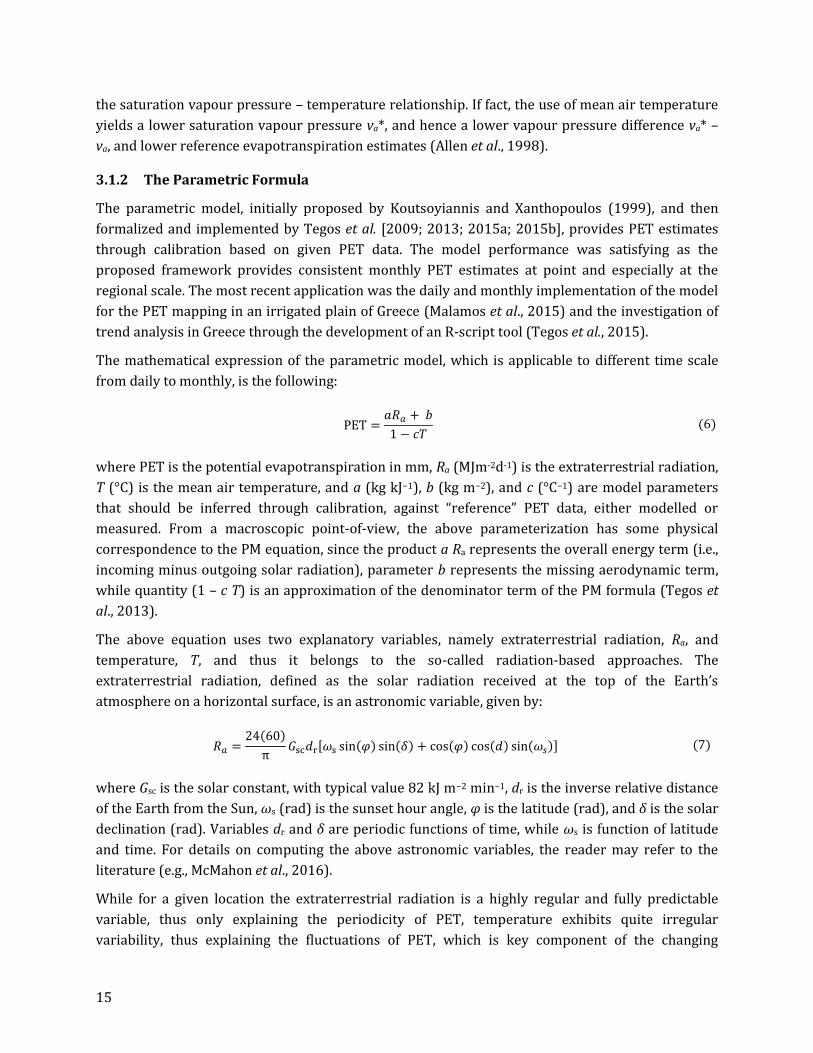
Figure 7. Ranges of coefficient of determination for the linear regression functions of monthly
reference PET against Ra and T, and the nonlinear parametric model. ......................................................... 24
Figure 8. CLIMWAT stations with negative NSE. ...................................................................................................... 26
Figure 9. Normal probability plot of the empirical distribution function of the mode residuals using
Weibull plotting positions against normal distribution function N (0, 0.7), for stations with negative
NSE............................................................................................................................................................................................... 27
Figure 10. Residuals vs parametric PET for stations with negative NSE. ...................................................... 27
Figure 11. Residuals vs. humidity (a) and wind speed (b) for stations with negative NSE. ................... 28
Figure 12. Distribution of NSE across CLIMWAT stations. ................................................................................... 30
Figure 13. Distribution of BIAS across CLIMWAT stations. ................................................................................. 31
Figure 14. Scatter plot of optimized parameters through the final data sample of 4088 stations
exhibiting positive NSE values. ........................................................................................................................................ 33
Figure 15. Spatial distribution of parameter a΄ over the globe. ......................................................................... 34
Figure 16. Spatial distribution of parameter c΄ over the globe. .......................................................................... 35
Figure 17. Mean annual Penman-Monteith potential evapotranspiration (symbols) for the 39 CIMIS
stations against the parametric model and the other four methods ................................................................ 45
Figure 18. Scatter plots of parameters against latitude and elevation ............................................................ 49
Figure 19 Study area and the CIMIS Stations used for spatial analysis ......................................................... 52
Figure 20 Parameters maps produced by the IDW method, for the California region ............................. 54
Figure 21 CLIMWAT meteorological stations network. ........................................................................................ 57
Figure 22 Eurasia PET map for August (PET: mm/day) ....................................................................................... 58
Figure 23 North America PET map for May- South America PET map for January (PET: mm/day).. 58
Figure 24 Africa/Oceania PET map for January-Oceania PET for December (PET: mm/day).............. 59
Figure 25 Monthly PM point vs RASPOTION estimate (Davis Station) ........................................................... 60
Figure 26. Annual PET at Ioannina ................................................................................................................................. 66
Figure 27. Annual PET at Kerkyra .................................................................................................................................. 66
Figure 28. Annual PET at Larissa .................................................................................................................................... 66
Figure 29. Annual PET at Lemnos ................................................................................................................................... 67
Figure 30. Study Area- meteorological stations locations .................................................................................... 68
Figure 31. Inter-annual temperature variability ...................................................................................................... 69
Figure 32. Study Area- locations of meteorological stations ............................................................................... 69
Figure 33. Annual PET variation ..................................................................................................................................... 70
Figure 34. The Arta plain along with the study area and the agrometeorological stations network . 72
Figure 35. BSS PET maps for Julian dates 105, 135, 162, 199, 229, 259 of year 2015 ............................. 75
Figure 36. IDW PET maps for Julian dates 105, 135, 162, 199, 229, 259 of year 2015 ............................ 76
Figure 37. Study Area ........................................................................................................................................................... 79
Figure 38. PET daily spatial variability ......................................................................................................................... 80
Figure 39. PET monthly variability ................................................................................................................................ 82
1
1 Introduction
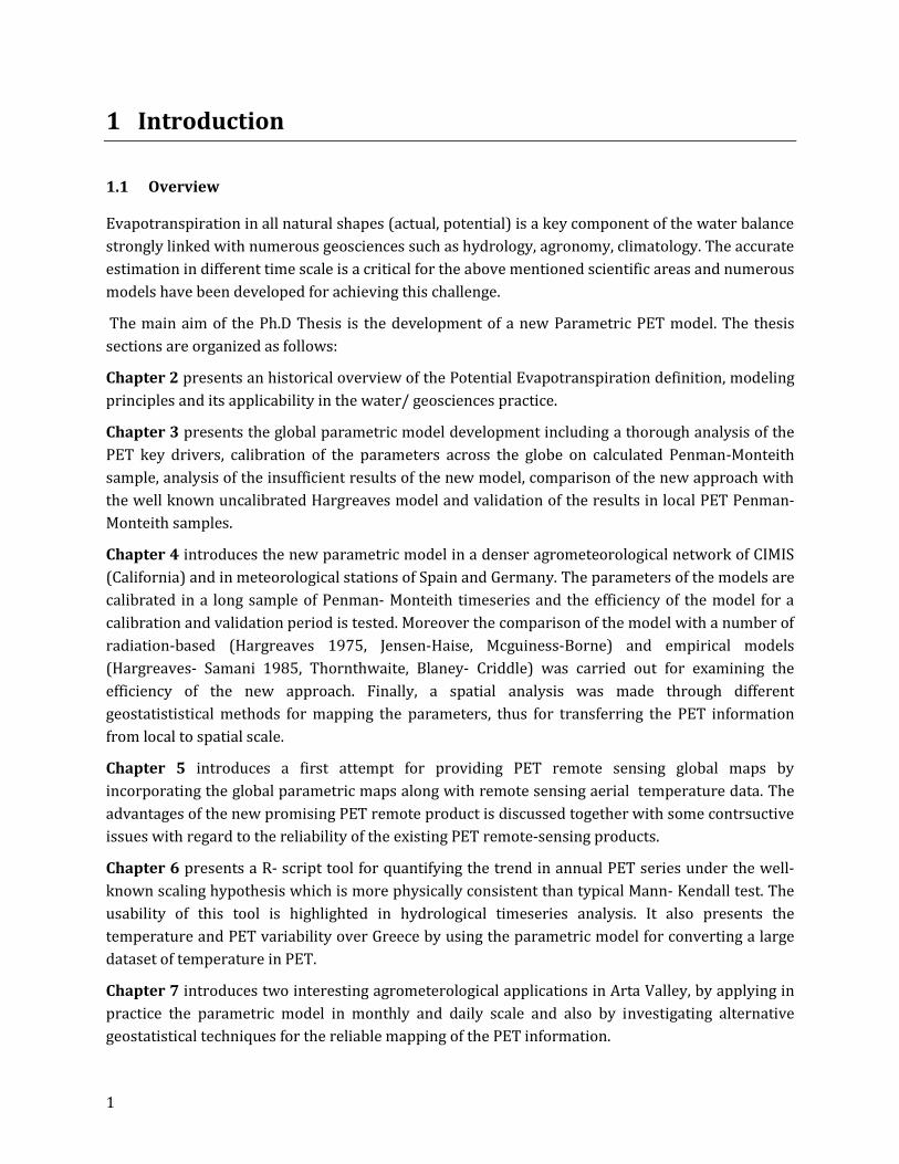
1.1 Overview
Evapotranspiration in all natural shapes (actual, potential) is a key component of the water balance
strongly linked with numerous geosciences such as hydrology, agronomy, climatology. The accurate
estimation in different time scale is a critical for the above mentioned scientific areas and numerous
models have been developed for achieving this challenge.
The main aim of the Ph.D Thesis is the development of a new Parametric PET model. The thesis
sections are organized as follows:
Chapter 2 presents an historical overview of the Potential Evapotranspiration definition, modeling
principles and its applicability in the water/ geosciences practice.
Chapter 3 presents the global parametric model development including a thorough analysis of the
PET key drivers, calibration of the parameters across the globe on calculated Penman-Monteith
sample, analysis of the insufficient results of the new model, comparison of the new approach with
the well known uncalibrated Hargreaves model and validation of the results in local PET Penman-
Monteith samples.
Chapter 4 introduces the new parametric model in a denser agrometeorological network of CIMIS
(California) and in meteorological stations of Spain and Germany. The parameters of the models are
calibrated in a long sample of Penman- Monteith timeseries and the efficiency of the model for a
calibration and validation period is tested. Moreover the comparison of the model with a number of
radiation-based (Hargreaves 1975, Jensen-Haise, Mcguiness-Borne) and empirical models
(Hargreaves- Samani 1985, Thornthwaite, Blaney- Criddle) was carried out for examining the
efficiency of the new approach. Finally, a spatial analysis was made through different
geostatististical methods for mapping the parameters, thus for transferring the PET information
from local to spatial scale.
Chapter 5 introduces a first attempt for providing PET remote sensing global maps by
incorporating the global parametric maps along with remote sensing aerial temperature data. The
advantages of the new promising PET remote product is discussed together with some contrsuctive
issues with regard to the reliability of the existing PET remote-sensing products.
Chapter 6 presents a R- script tool for quantifying the trend in annual PET series under the well-
known scaling hypothesis which is more physically consistent than typical Mann- Kendall test. The
usability of this tool is highlighted in hydrological timeseries analysis. It also presents the
temperature and PET variability over Greece by using the parametric model for converting a large
dataset of temperature in PET.
Chapter 7 introduces two interesting agrometerological applications in Arta Valley, by applying in
practice the parametric model in monthly and daily scale and also by investigating alternative
geostatistical techniques for the reliable mapping of the PET information.

2
Chapter 8 summarises the conclusion of the Ph.D thesis works its innovation for different
disciplines, unresolved scientific issues and future objectives for further research.
In the Appendix the peer-review publications are listed along with detailed citations per article.
1.2 Scientific innovations of the thesis
The major innovative queries examined as part of this Ph.D thesis outlined below:
Which are the key meteorological drivers for assessing the PET in large areas?
An extended global statistical analysis was carried out for investigating the relationship between PET,
mean temperature, radiation, humidity and wind velocity. PET is strongly correlated with mean
temperature and radiation but in some cases the humidity and velocity could improve the reliability of
the PET estimate.
Given the high data demanding dataset for estimating the reliability of PET, can we
introduce parsimony and physical constraints for its quantification?
The major peer review publications as part of the thesis outcomes are available which represent: a)
The global parametric model in a sample of 4088 FAO stations and b) The development of the
parametric model in the CIMIS network in California.
What is the main benefit of the new parametric model against the other radiation or
temperature-based methods?
It is resulted that the performance of the new model is satisfactorily outperforming all the other
radiation- based methods or temperature methods that have been applied. Specifically, the new
parametric model is preferable to the most well-known temperature-based method which is the
Hargeaves-Samani.
Which is the optimal geostatistical model for transferring the local PET estimate in spatial
scale?
A typical problem in engineering hydrology is the conversion of the points estimate to spatial
information. Therefore a number of the geostatistical tools (IDW, Kriging, NN, BSS) were compared in
order to find out the most applicable model in representing the PET in spatial scale. IDW the most
simplistic, seems to be the optimal model.
What are the changes of annual PET and how can we quantify the trend?
An R-script had been developed in order to investigate the annual PET trends under the scaling
hypotheses which, given the ubiquitous presence in meteorological timeseries, have physical
constraints.
Which are the practical uses of a new PET model in the area of hydrological and agronomic
engineering?

3
A number of innovative case studies have outlined the usability of the new parsimonious PET model.
Specifically, the use of the model in the quick and reliable conversion of the mean temperature in PET
estimates and the study of the long term changes and its usability in agronomic applications.
What are the major incidental contributions and moderate innovations of this thesis?
During the development of the global parametric model in a limited number of areas, an influence of
the humidity and/or the velocity had been detected and therefore more meteorological timeseries and
more explanatory variables (humidity and/or velocity) are required for developing more robust PET
expressions.

4
2 Overview of PET models
2.1 The potential evapotranspiration process
Potential evapotranspiration (PET) is key input in water resources, agricultural and environmental
modelling. For many decades, numerous approaches have been proposed for the consistent
estimation of PET at several time scales of interest. Accurate estimation of evapotranspiration has
gained scientific interest due to high importance in hydrological modelling, irrigation planning and
water resources management. According to Farquhar and Roderick (2007), changes in evaporative
demand affect fresh water supplies and have impact on agriculture, the biggest consumer of fresh
water.
Evaporation can be viewed both as energy (heat) exchange and an aerodynamic process. According
to the energy balance approach, the net radiation at the Earth’s surface Rn is mainly transformed to
latent heat flux, Λ, and sensible heat flux to the air, H.
The evaporation rate, expressed in terms of mass per unit area and time (e.g. kg/m2/d), is given by
the ratio E΄ := Λ / λ, where λ is the latent heat of vaporization, with typical value 2460 kJ/kg. By
ignoring fluxes of lower importance, such as soil heat flux, the heat balance equation is solved for
evaporation, yielding:
(1)
where b := H / Λ is the co-called Bowen ratio. The estimation of b requires the measurement of
temperature at two levels (surface and atmosphere), as well as the measurement of humidity at the
atmosphere. On the other hand, the estimation of the net radiation Rn is based on a radiance
balance approach to determine the components Sn (Net short wave radiation) and Ln (Net long
wave radiation). Typical input data required (in addition to latitude and time of the year), are solar
radiation (direct and diffuse, or, in absence of them, sunshine duration data or cloud cover
observations), temperature and relative humidity. The net radiation also depends of surface
properties (i.e. albedo) and topographical characteristics, in terms of slope, aspect and shadowing.
From the aerodynamic viewpoint, evaporation is a mass diffusion process. In this context, the rate
of evaporation is related to the difference in the water vapor content of the air at two levels above
the evaporating surface and a function of the wind speed F(u) in the diffusion equation.
Theoretically, F(u) can be computed on the basis of elevation, wind velocity, aerodynamic
resistance and temperature. Yet, for simplicity it is usually given by empirical formulas, derived
through linear regression, for a standard measurement level of 2 meters. Penman (Penman, 1948)
combined the energy balance with the mass transfer approaches, thus allowing the use of
temperature, humidity and wind speed measurements at a single elevation. His classical formula for
computing evaporation from an open water surface is written as:

5
(2)
where Δ is the slope of saturated vapor pressure/temperature curve at equilibrium temperature
(hPa/K), γ is a psychrometrcic coefficient, with typical value 0.67 hPa/K, and D is the vapor
pressure deficit of the air (hPa), defined as the difference between the saturation vapor pressure es
and the actual vapor pressure ea, which are functions of temperature and relative humidity. We
remind that estimates the evaporation rate (mass per unit area per day), which is expressed in
terms of equivalent evaporation of water by dividing by the water density ρ (1000 kg/m3).
Penman’s method was extended to cropped surfaces, by accounting for various resistance factors,
aerodynamic and surface. As mentioned in the introduction, Monteith introduced the concept of the
so-called “bulk” surface resistance that describes the resistance of vapor flow through the
transpiring crop and evaporating soil surface.
It is therefore the Penman-Monteith formula (Monteith 1965, Monteith 1981) most recognized
globally, which is yet difficult to apply in data-scarce areas, since it requires simultaneous
observations of four meteorological variables (temperature, net duration, relative humidity, wind
velocity). For this reason, parsimonious models with minimum input data requirements are
strongly preferred. Typically, these have been developed and tested for specific hydroclimatic
conditions, but when they are applied in different regimes they provide much less reliable (and in
some cases misleading) estimates. Therefore, it is essential to develop generic methods that remain
parsimonious, in terms of input data and parameterization and this is part of this Ph.D thesis.
2.2 Historical overview of PET modelling
2.2.1 General
The accurate estimation of evapotranspiration has a great importance in hydrological modeling,
irrigation planning and water resources management.
Figure 1 presents the historical milestones in developing evapotraspiration definition and physical
modelling focusing in the two last centuries.

6
Figure 1. PET definitions milestones as presented in McMahon et al. 2016
The starting point was the first “common-sense” definitions introducing by Aristotle (Koutsoyiannis
et al. 2007). His views in this fundamental work “Meterologika” encompasses a clear understanding
for the phase change of water and the energy exchange. He referred that “… the sun causes the
moisture to rise; this is similar to what happens when water is heated by fire” (Meteorologica, II.2,
355a 15). “… the vapour that is cooled, because of lack of heat in the area where it lies, condenses
and turns from air into water; and after the water has formed in this way it falls down again to the
earth” (ibid., I.9, 346b 30). Later Perrault (1611–1680) is credited with having made the first
experimental measurement of evaporation, though in fact what he measured was sublimation by
recording the loss of weight of a block of ice through time. The first direct measurement of the
evaporation of liquid water was carried out by Edmund Halley in 1686 when he measured the loss
of water from a heated pan. Surprisingly, Halley appears not to understand that the temperature is
good predictor and key driver of evaporation loss as shown in Figure 2.

7
Figure 2. Evaporation vs temperature plot from Halley’s experiment (source McMahon et al. 2016)
Dalton has become universally recognized as one of the foreseen scientist in the development of
evaporation theory since he referred that “the evaporating force must be universally equal to that of
the temperature of the water, diminished by that already existing in the atmosphere”. The water
existing in the atmosphere he refers to as the ‘force of the vapour,’ effectively relative humidity.
After Dalton’s contribution in explaining evaporation as a physical phenomenon, Penman and
Monteith later introduced the most recognized physical approaches until nowadays and more
informatios are presented later herein.
More than 50 important evapotranspiration models can be found in literature (Lu et al., 2005,
McMahon et al. 2013) which can be grouped into seven categories: (i) empirical, (ii) water budget
(iii) energy budget, (iv) mass transfer, (v) combination, (vi) radiation and (vii) measurement (Xu
and Singh, 2000).
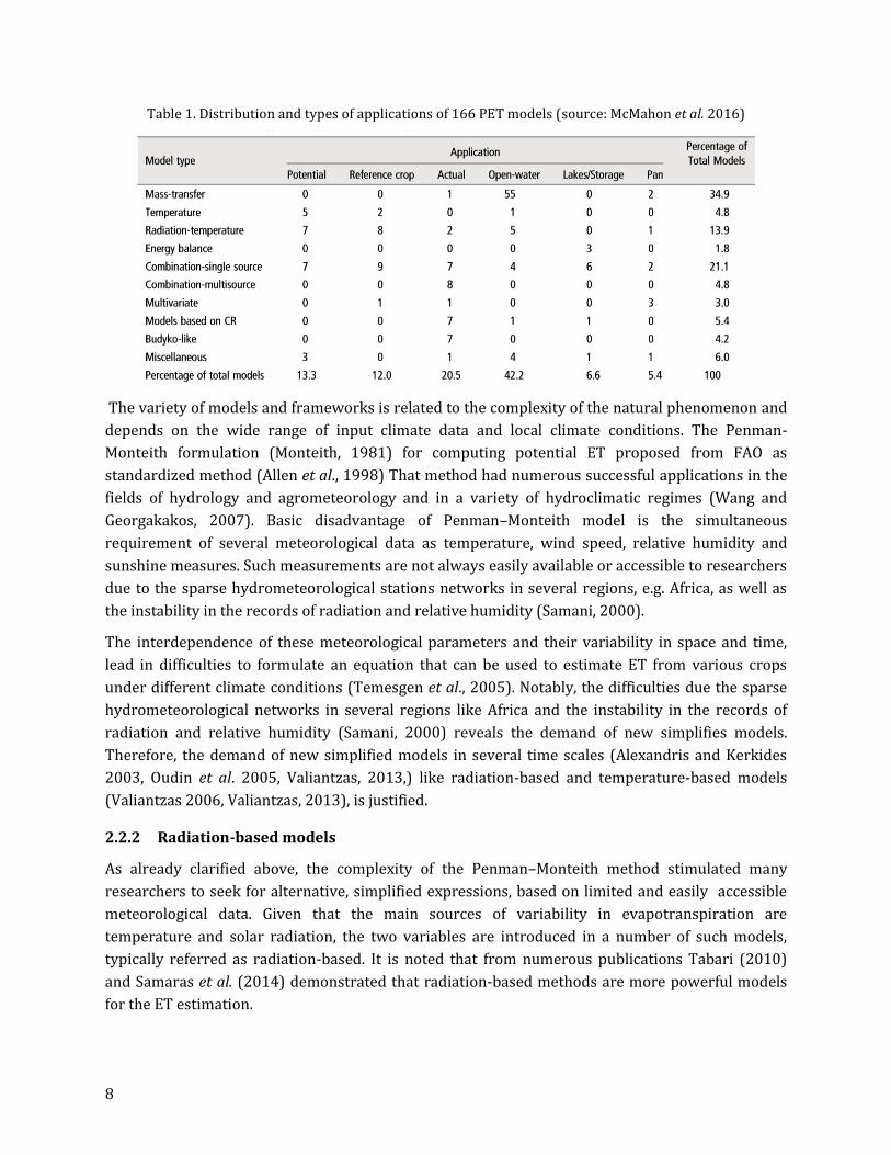
The recently review work by McMahon et al. 2016 has identified a total number of 166 models
categorizing into six classes (Table 1): potential evaporation, reference evaporation, actual
evaporation in terrestrial environments, open-water evaporation, deep lakes, and pan evaporation.
The models therein are further typed into the following 10 classes: models based on mass-transfer
(so-called Dalton equation), temperature models, radiation-temperature models, energy balance
methods, single-source (vegetation, soil, or water) combination methods, multisource combination
methods, multivariate models, models based on the Complementary Relationship, Budyko-like
models, and miscellaneous models.
8
Table 1. Distribution and types of applications of 166 PET models (source: McMahon et al. 2016)
The variety of models and frameworks is related to the complexity of the natural phenomenon and
depends on the wide range of input climate data and local climate conditions. The Penman-
Monteith formulation (Monteith, 1981) for computing potential ET proposed from FAO as
standardized method (Allen et al., 1998) That method had numerous successful applications in the
fields of hydrology and agrometeorology and in a variety of hydroclimatic regimes (Wang and
Georgakakos, 2007). Basic disadvantage of Penman–Monteith model is the simultaneous
requirement of several meteorological data as temperature, wind speed, relative humidity and
sunshine measures. Such measurements are not always easily available or accessible to researchers
due to the sparse hydrometeorological stations networks in several regions, e.g. Africa, as well as
the instability in the records of radiation and relative humidity (Samani, 2000).
The interdependence of these meteorological parameters and their variability in space and time,
lead in difficulties to formulate an equation that can be used to estimate ET from various crops
under different climate conditions (Temesgen et al., 2005). Notably, the difficulties due the sparse
hydrometeorological networks in several regions like Africa and the instability in the records of
radiation and relative humidity (Samani, 2000) reveals the demand of new simplifies models.
Therefore, the demand of new simplified models in several time scales (Alexandris and Kerkides
2003, Oudin et al. 2005, Valiantzas, 2013,) like radiation-based and temperature-based models
(Valiantzas 2006, Valiantzas, 2013), is justified.
2.2.2 Radiation-based models
As already clarified above, the complexity of the Penman–Monteith method stimulated many
researchers to seek for alternative, simplified expressions, based on limited and easily accessible
meteorological data. Given that the main sources of variability in evapotranspiration are
temperature and solar radiation, the two variables are introduced in a number of such models,
typically referred as radiation-based. It is noted that from numerous publications Tabari (2010)
and Samaras et al. (2014) demonstrated that radiation-based methods are more powerful models
for the ET estimation.
9
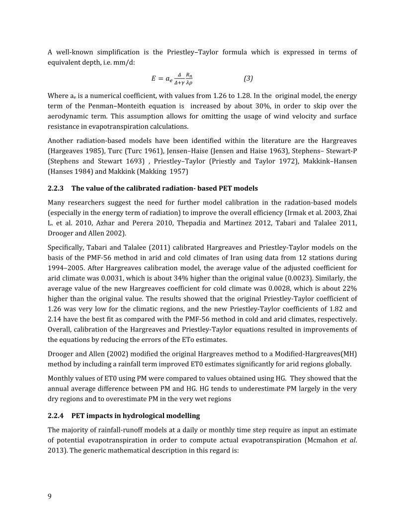
A well-known simplification is the Priestley–Taylor formula which is expressed in terms of
equivalent depth, i.e. mm/d:
(3)
Where ae is a numerical coefficient, with values from 1.26 to 1.28. Ιn the original model, the energy
term of the Penman–Monteith equation is increased by about 30%, in order to skip over the
aerodynamic term. This assumption allows for omitting the usage of wind velocity and surface
resistance in evapotranspiration calculations.
Another radiation-based models have been identified within the literature are the Hargreaves
(Hargeaves 1985), Turc (Turc 1961), Jensen–Haise (Jensen and Haise 1963), Stephens– Stewart-P
(Stephens and Stewart 1693) , Priestley–Taylor (Priestly and Taylor 1972), Makkink–Hansen
(Hanses 1984) and Makkink (Makking 1957)
2.2.3 The value of the calibrated radiation- based PET models
Many researchers suggest the need for further model calibration in the radation-based models
(especially in the energy term of radiation) to improve the overall efficiency (Irmak et al. 2003, Zhai
L. et al. 2010, Azhar and Perera 2010, Thepadia and Martinez 2012, Tabari and Talalee 2011,
Drooger and Allen 2002).
Specifically, Tabari and Talalee (2011) calibrated Hargreaves and Priestley-Taylor models on the
basis of the PMF-56 method in arid and cold climates of Iran using data from 12 stations during
1994–2005. After Hargreaves calibration model, the average value of the adjusted coefficient for
arid climate was 0.0031, which is about 34% higher than the original value (0.0023). Similarly, the
average value of the new Hargreaves coefficient for cold climate was 0.0028, which is about 22%
higher than the original value. The results showed that the original Priestley-Taylor coefficient of
1.26 was very low for the climatic regions, and the new Priestley-Taylor coefficients of 1.82 and
2.14 have the best fit as compared with the PMF-56 method in cold and arid climates, respectively.
Overall, calibration of the Hargreaves and Priestley-Taylor equations resulted in improvements of
the equations by reducing the errors of the ETo estimates.
Drooger and Allen (2002) modified the original Hargreaves method to a Modified-Hargreaves(MH)
method by including a rainfall term improved ET0 estimates significantly for arid regions globally.
Monthly values of ET0 using PM were compared to values obtained using HG. They showed that the
annual average difference between PM and HG. HG tends to underestimate PM largely in the very
dry regions and to overestimate PM in the very wet regions
2.2.4 PET impacts in hydrological modelling
The majority of rainfall-runoff models at a daily or monthly time step require as input an estimate
of potential evapotranspiration in order to compute actual evapotranspiration (Mcmahon et al.
2013). The generic mathematical description in this regard is:

10
) (4)
Where ETAct is the estimated actual daily evapotranspiration (mmday-1), SM is a proxy soil moisture
level for the given day (mm) and ETPET is the daily potential evaporation (mmday-1). Due to local
climatic conditions especially in arid catchments actual evapotranspiration is limited by soil
moisture with the potential evapotranspiration becoming more important in wet catchments where
soil moisture is not limiting.
Seiller and Anctil (2016) were assessed the performance of the hydrological modeling under
observed and projected climate conditions on natural catchments in Canada and Germany by using
as input twenty-four potential evapotranspiration formulas (Penman, Penman-Monteith, FAO56 P-
M, Priestley- Taylor, Kimberly-Penman, Thom-Oliver, Thornthwaite, Blaney and Criddley, Hamon,
Romanenko, Linacre, MOHYSE, HSAMI, Kharrufa, Wendling – WASim, Turc, Jensen and Haise ,
McGuinness and Bordne, Hargreaves and Samani, Doorenbos and Pruit, Abtew, Makkink, Oudin,
Baier and Robertson).
The 24 PET formulas produced large dissimilarities in the estimated PET in terms of quantity and
shape. Conclusively, the combinational formulas proposed very similar shape and quantity,
temperature-based formulas produced the largest spectrum of quantity and the Radiation-based
formulas fell somewhere in between the other two classes namely combinational and temperature-
based. These differences affected in several ways the resulting simulated discharge time series.
Overall, the authors concluded that it was difficult to identify an ultimate PET formula for a
hydrological modelling point of view, but it could be recommended avoiding temperature-based
Blaney and Criddley and MOHYSE.
Another one critical outcome was the results showed that spread of the hydrological response was
smaller for the combinational formulas than for temperature-based and radiation-based equations,
revealing a higher stability of these combinational formulas.
Birhanu et al. (2018) were applied five hydrological models of increasing complexity (GR4J,
SIMHUD, CAT, TANK, SAC-SMA) by inputting 12 Potential Evapotranspiration (Abtew, Blaney-
Criddle, Chapman Australian, Granger Gray, Hamon, Hargeaves-Samani, Makkink, Matt
Shuttleworth, Penman, Penman- Monteith, Priestley-Taylor, Turc) estimation methods of different
input-data requirements in order to assess their effect on model performance, optimized
parameters and robustness. The study area located over a set of 10 catchments in South Korea.
The main outcomes of the study outlined below:
The hydrological models’ performance was satisfactory for each PET input in the calibration
and validation periods for all of the tested catchments.
The hydrological models performances were found to be insensitive to the 12 PET.
Identical behavioural similarities and Dimensionless Bias were observed in all of the tested
catchments.
For the hydrological models, lack of robustness and higher dimensionless Bias were found
for high and low flow as well as for the Hamon PET input.

11
The complexity of the hydrological models structure and the PET estimation methods did
not necessarily enhance model performance and robustness.
The model performance and robustness were found to be mainly dependent on extreme
hydrological conditions, including high and low flow, rather than complexity;
The simplest hydrological model and PET estimation method could perform better if
reliable hydro-meteorological datasets are applied.
2.2.5 Outstanding issues
According to the fundamental work by Mcmahon et al. 2013 a number of issues regarding the
evapotranspiration are still outstanding and outlined below:
Hard-wired potential evaporation estimates at AWSs; The authors stated that: ”Some
commercially available AWSs, in addition to providing values of the standard climate
variables, output an estimate of Penman evaporation or Penman–Monteith evaporation. For
practitioners, this will probably be the data of choice rather than recomputing Penman or
Penman–Monteith evaporation estimates from basic principles. However, users need to
understand the methodology adopted and check the values of the parameters and functions
(e.g. albedo, wind function, ra and rs) used in the AWS evaporation computation”
Estimating evaporation without wind data; Authors mentioned that “Many countries do not
have access to historical wind data to compute potential evaporation”
Estimating evaporation without at-site data; The authors mentioned that “Where at-site
meteorological or pan evaporation data are unavailable, it is recommended that evaporation
estimates be based on data from a nearby weather station that is considered to have similar
climate and surrounding vegetation conditions to the site in question”.
Dealing with a climate change environment: increasing annual air temperature but
decreasing pan evaporation rates;
Daily meteorological data average over 24h or day-light hours only; The authors stated that
“An issue that arose during this project relates to whether or not daily meteorological data
used in evaporation equations should be averaged over a 24h daily period or averaged during
daylight hours when evaporation is mainly, but not only”
Uncertainty in evaporation estimates. The authors refers that “We describe several models
for estimating actual and potential evaporation. These models vary in complexity and in data
requirements. In selecting an appropriate model, analysts should consider the uncertainty in
alternative methods.”
In this PhD thesis the majority of the above mentioned critical points are considered in order to
introduce new insights in the PET assessment.
12
3 Global Parametric model development
The need of parsimonious model structure is essential in several fields of water resources sciences
(Koutsoyiannis, 2009; Koutsoyiannis, 2014). This refers both to the model structure and to the
input data, which should be easily available. Most of simplified formulas fail to describe the
phenomenon of evapotranspiration due to its high complexity and the varying local climate
conditions. Thus, the idea of replacing some variables and constants used in the standard Penman-
Monteith (PM) formula by a number of parameters which are regionally varying and estimated through
calibration from a reference evapotranspiration sample, constitutes a new appealing strategy for
evapotranspiration estimation.
3.1 Introduction
Evaporation, which is an overall term covering all processes in which liquid water is transferred as
water vapour to the atmosphere—definition already provided by ancient Greek philosophers
(Koutsoyiannis et al. 2007)—is crucial element of multiple disciplines and an essential input of
hydrological modelling, water resources management, irrigation planning, and climatological
studies. Numerous efforts are reported in the literature, presenting different expressions of
evaporation (including actual, potential, reference crop, and pan evaporation), based on different
types of data. McMahon et al. (2013, 2016) provide a major discussion of the background theory
and definitions, as well as a critical assessment of the models developed so far.
Here, the concept of potential evapotranspiration, PET is highlighted, which is a theoretical quantity
considered as “the rate at which evapotranspiration would occur from a large area completely and
uniformly covered with growing vegetation, which has access to an unlimited supply of soil water,
and without advection or heating effects” (Dingman, 1994). Since PET depends on soil properties, a
better defined term is the so-called reference crop evapotranspiration, introduced by Doorenbos
and Pruitt (1977), and typically denoted as ET0, which refers to the evapotranspiration from a
standardized vegetated surface (i.e., actively growing and completely shading grass of 0.12 m
height, surface resistance 70 s m−1, and albedo = 0.23). The globally accepted method for consistent
estimation of PET is the Penman-Monteith (herein referred to as PM) equation, as formalized by the
Food and Agriculture Organization (FAO), which is physically-based, and is therefore used as
standard for comparisons with other, more simple approaches (Allen et al. 1989). The major
drawback for the generalized application of the PM method worldwide is the need of simultaneous
measurements of four meteorological variables (air temperature, wind speed, relative humidity,
and net radiation or, alternatively, sunshine duration), at the desirable spatial and temporal
resolution.
To overcome the data requirements of the PM formula, a number of alternative approaches have
been developed, which are typically classified into temperature-based and radiation-based; the
former use only temperature observations, which are dense and easily accessible, while the latter
also use values of extraterrestrial radiation (which is, in fact, periodic function of latitude and day of

13
the year). For many decades, such approaches have been widely applied for PET modelling
worldwide using the standard “literature” values of the parameters involved in their governing
equations. However, since these have been developed for specific studies, locations, and climatic
conditions (Xu and Singh, 2001), their applicability outside of these distinct conditions usually
result in unreliable predictions, introducing significant bias in PET estimations. For this reason, and
particularly in the last years, significant attention is payed to local calibrations of empirical PET
models, either by using direct PET observations at the field scale (e.g., lysimeter measurements)
and/or against simulated PET data, provided by the PM formula. One of the first attempts is
reported by Allen and Pruit (1986), who calibrated and validated the Blaney-Criddle model against
PM data, using local wind function and taking advantage of daily lysimeter measurements of alfalfa
evapotranspiration. Similar calibration approaches were employed for all of the widespread PET
formulas, such as the Thornthwaite, Blaney-Criddle and Priestley-Taylor (e.g., Amatya et al., 1995;
Mohawesh, 2010; Sentelhas et al., 2010), and other empirical expressions as well (e.g., Oudin et al.,
2005). Many recent publications also focus on the re-evaluation of the sole parameter of the
Hargreaves equation against regional data, for a range of climatic regimes (Gavilán et al., 2006;
Fooladmand and Haghighat, 2007; Tabari and Talaee, 2011; Hu et al., 2011; Haslinger and Bartsch,
2016).
Although the spatial resolution and accuracy of meteorological data over the extended areas of the
globe is not sufficient, current advances in remote sensing technologies allowed quite reliable
estimations of PET by combining satellite and ground information (Choudhury, 1997). Since
gridded data of meteorological inputs and canopy characteristics is now easily accessible, several
researchers employed PET estimations at large spatial scales, up to global (Allen et al., 2007; 2011;
Mu et al., 2007; 2011), by employing scaling and interpolation techniques of varying physical
complexity (Vinukollu et al. 2011).
Tegos et al. (2013; 2015) calibrated a simplified radiation-based expression of the PM formula,
using monthly meteorological data from a large number of stations over Greece and California,
respectively. In both areas, the proposed formula, which contains either three or two free
parameters, clearly outperformed other widely used methods, such as Hargreaves and Samani
(1985), Oudin et al. (2005), and Jensen and Haise (1963), as modified by McGuinness and Bordne
(1972). Malamos et al. (2015) also employed the parametric model at the daily scale, in the context
of PET mapping over the irrigated plain of Arta, Western Greece.
In the following chapters, the simplified (i.e. with two parameters) expression of the
aforementioned model over the globe is presented, by inferring its parameters through calibration
against given Penman-Monteith values (next referred to as reference PET or ET0). The
meteorological inputs and ET0 data are retrieved by the FAO CLIMWAT database that provides
monthly climatic information at 4300 locations worldwide. A preliminary analysis of these data
allowed explaining the major drivers of PET over the globe and across seasons. An extended
analysis of the model inputs and outputs was performed, including the production of global maps of
optimized model parameters and associated performance metrics, as well as comparisons with a
widely known formula by Hargreaves and Samani (1985). Finally, the interpolated values of the
14
optimized parameter values to validate the predictive capacity of the model against detailed
meteorological data was used, in terms of monthly time series, at several stations worldwide. The
results are very encouraging, since even with the use of abstract climatic information for its
calibration, the model generally ensures very reliable PET estimations. However, we have detected
few cases where the model systematically fails to reproduce the reference PET, particularly across
tropical areas. Except for these specific areas, the parameter estimations through the derived maps
can be directly employed within the proposed formula, at both point and regional scales.
3.1.1 Theoretical Background
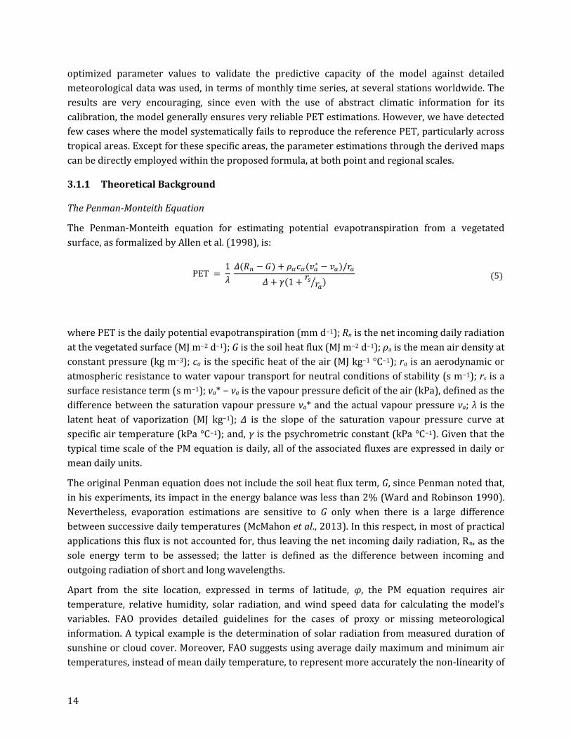
The Penman-Monteith Equation
The Penman-Monteith equation for estimating potential evapotranspiration from a vegetated
surface, as formalized by Allen et al. (1998), is:
(5)
where PET is the daily potential evapotranspiration (mm d−1); Rn is the net incoming daily radiation
at the vegetated surface (MJ m−2 d−1); G is the soil heat flux (MJ m−2 d−1); ρa is the mean air density at
constant pressure (kg m−3); ca is the specific heat of the air (MJ kg−1 °C−1); ra is an aerodynamic or
atmospheric resistance to water vapour transport for neutral conditions of stability (s m−1); rs is a
surface resistance term (s m−1); va* − va is the vapour pressure deficit of the air (kPa), defined as the
difference between the saturation vapour pressure va* and the actual vapour pressure va; λ is the
latent heat of vaporization (MJ kg−1); Δ is the slope of the saturation vapour pressure curve at
specific air temperature (kPa °C−1); and, γ is the psychrometric constant (kPa °C−1). Given that the
typical time scale of the PM equation is daily, all of the associated fluxes are expressed in daily or
mean daily units.
Τhe original Penman equation does not include the soil heat flux term, G, since Penman noted that,
in his experiments, its impact in the energy balance was less than 2% (Ward and Robinson 1990).
Nevertheless, evaporation estimations are sensitive to G only when there is a large difference
between successive daily temperatures (McMahon et al., 2013). In this respect, in most of practical
applications this flux is not accounted for, thus leaving the net incoming daily radiation, Rn, as the
sole energy term to be assessed; the latter is defined as the difference between incoming and
outgoing radiation of short and long wavelengths.
Apart from the site location, expressed in terms of latitude, φ, the PM equation requires air
temperature, relative humidity, solar radiation, and wind speed data for calculating the model’s
variables. FAO provides detailed guidelines for the cases of proxy or missing meteorological
information. A typical example is the determination of solar radiation from measured duration of
sunshine or cloud cover. Moreover, FAO suggests using average daily maximum and minimum air
temperatures, instead of mean daily temperature, to represent more accurately the non-linearity of
15
the saturation vapour pressure – temperature relationship. If fact, the use of mean air temperature
yields a lower saturation vapour pressure va*, and hence a lower vapour pressure difference va* –
va, and lower reference evapotranspiration estimates (Allen et al., 1998).
3.1.2 The Parametric Formula
The parametric model, initially proposed by Koutsoyiannis and Xanthopoulos (1999), and then
formalized and implemented by Tegos et al. [2009; 2013; 2015a; 2015b], provides PET estimates
through calibration based on given PET data. The model performance was satisfying as the
proposed framework provides consistent monthly PET estimates at point and especially at the
regional scale. The most recent application was the daily and monthly implementation of the model
for the PET mapping in an irrigated plain of Greece (Malamos et al., 2015) and the investigation of
trend analysis in Greece through the development of an R-script tool (Tegos et al., 2015).
The mathematical expression of the parametric model, which is applicable to different time scale
from daily to monthly, is the following:
(6)
where PET is the potential evapotranspiration in mm, Ra (MJm-2d-1) is the extraterrestrial radiation,
T (°C) is the mean air temperature, and a (kg kJ−1), b (kg m−2), and c (°C−1) are model parameters
that should be inferred through calibration, against “reference” PET data, either modelled or
measured. From a macroscopic point-of-view, the above parameterization has some physical
correspondence to the PM equation, since the product a Ra represents the overall energy term (i.e.,
incoming minus outgoing solar radiation), parameter b represents the missing aerodynamic term,
while quantity (1 – c T) is an approximation of the denominator term of the PM formula (Tegos et
al., 2013).
The above equation uses two explanatory variables, namely extraterrestrial radiation, Ra, and
temperature, T, and thus it belongs to the so-called radiation-based approaches. The
extraterrestrial radiation, defined as the solar radiation received at the top of the Earth’s
atmosphere on a horizontal surface, is an astronomic variable, given by:
(7)
where Gsc is the solar constant, with typical value 82 kJ m−2 min−1, dr is the inverse relative distance
of the Earth from the Sun, ωs (rad) is the sunset hour angle, φ is the latitude (rad), and δ is the solar
declination (rad). Variables dr and δ are periodic functions of time, while ωs is function of latitude
and time. For details on computing the above astronomic variables, the reader may refer to the
literature (e.g., McMahon et al., 2016).
While for a given location the extraterrestrial radiation is a highly regular and fully predictable
variable, thus only explaining the periodicity of PET, temperature exhibits quite irregular
variability, thus explaining the fluctuations of PET, which is key component of the changing

16
hydrological cycle, at all temporal scales, from daily to annual and even larger ones, i.e. overannual
(Koutsoyiannis, 2013). Following FAO recommendations, the advantage from minimum and
maximum daily temperature data was taken, thus estimating the temperature term by the average:
(8)
This expression may be particularly useful in cases when records of mean daily temperature are
missing, while average minimum (Tmin) and maximum temperature (Tmax) values are available.
3.1.3 Modified Parametric Model
It is well-known that the variability of daily and, even more, monthly PET is relatively small, if
compared to other hydrometeorological variables, such as precipitation and runoff. For this reason,
when attempting to estimate the model parameters a, b, and c through calibration, it is quite easy to
achieve very high values of goodness-of-fitting criteria (e.g. efficiency), through combinations of
parameter values that do not have physical sense. Additional uncertainty arises when the actual
PET data is little informative to support the inference of the three parameters, e.g. due to limited
length of associated meteorological data. In this respect, to avoid uncertainties due to “blind”
calibration approaches or overfitting (Efstratiadis and Koutsoyiannis, 2010), we propose using the
more parsimonious expression (also considering the minimum and maximum temperature, instead
of the mean daily one):
(9)
which contains two instead of three parameters (parameter a΄ in the numerator and parameter c΄ in
the denominator). Apparently, in the context of a calibration exercise using alternative expressions
(6) and (7), the optimized values of c and c΄ should be different.
The modified parameterization of the above equation resembles the well-known approach by
Priestley and Taylor (1972), who developed a PET formula based on the original PM equation, but
without the aerodynamic component; the latter was indirectly accounted by increasing the energy
term by a factor of 1.26. For simplicity, this factor is generally considered as constant; however,
several researchers have demonstrated that this exhibits quite significant seasonal and spatial
variability (McMahon et al. 2013).
3.1.4 The CLIMWAT Database: Preliminary Analysis
Database Overview
The CLIMWAT 2.0 database is a joint initiative by the Water Development and Management Unit
and the Climate Change and Bioenergy Unit of FAO (1993), which provides average monthly
climatic data at 4300 stations (Figure 3, blue points), well-distributed worldwide. These data
include monthly mean values of mean daily maximum and minimum temperature (°C), daily
relative humidity (%), wind speed (km day-1), daily sunshine duration (h), daily solar radiation

17
(MJ/m2), monthly rainfall, gross and effective (mm), as well as mean monthly ET0 estimations
through the Penman-Monteith formula.
The exceptionally large sample of climatic data allows for extracting useful conclusions about the
major drivers of PET over the globe. In this context, a comprehensive statistical analysis of
reference PET data against the available meteorological variables, at both the annual and monthly
scales was made.
Figure 3. Food and Agriculture Organization (FAO CLIMWAT) hydrometeorological network (dark areas
indicate high altitudes).
Which Meteorological Drivers Explain Mean Annual PET over the Globe?
In order to answer this question, the reference PET (i.e. ET0) data against the four meteorological
variables that are embedded in the Penman-Monteith equation was plotted, i.e. solar radiation,
mean temperature estimated from Equation (7), relative humidity and wind speed, at the annual
scale, and fitted the most suitable regression model.
Figure 4 illustrates that mean annual ET0 over the globe is highly correlated with mean annual solar
radiation and temperature, particularly when considering power-type or exponential regression
functions. As expected, mean annual ET0 is negatively correlated with mean relative humidity, while
it seems uncorrelated to wind speed. It is worth mentioning that as the solar radiation and
temperature increase, the variance of ET0 increases significantly. Therefore, in order to reduce

18
heteroscedasticity effects, it is essential considering at least two explanatory variables in the
context of empirical PET modelling.
Figure 4 also demonstrates the variability of mean annual ET0 against mean annual sunshine
duration and annual extraterrestrial radiation, which are typically used instead of solar radiation, in
PET estimations (given that solar radiation observations are generally sparse, due to the cost of
associated equipment, i.e. pyranometers, radiometers or solarimeters). Surprisingly, the mean
annual sunshine duration is slightly less correlated with mean annual ET0 than extraterrestrial
radiation, although the former is expected to be better estimator of the actual solar energy received
in the Earth’s surface. This is a very important conclusion that confirms the suitability of radiation-
based approaches, using both temperature and extraterrestrial radiation as explanatory variables
of PET. However, it is essential remarking that the overall driver of PET and temperature as well is
net solar radiation, which is a portion of the extraterrestrial one. Furthermore, the correlation
between PET and temperature is so much significant only at coarse time scales, such as the annual
one, while its correlation with the solar radiation remains significant, at all temporal scales
(Lofgren et al., 2011).

19
Figure 4. Scatter plot of mean annuals of (a) solar radiation, (b) temperature, (c) relative humidity, (d) wind speed, (e) sunshine duration, (f) extraterrestrial radiation vs. mean annual ET0.
How Well do Extraterrestrial Radiation and Temperature Explain the Seasonal Patterns of PET?
The key assumption of radiation-based models is that PET follows the seasonal patterns of
extraterrestrial radiation, Ra, and temperature, T. In general, a loop-type shape exists between the
mean monthly PET and the two aforementioned variables, due to the influence of thermal inertia,
causing a delay in temperature changes against solar radiation changes across seasons. Apparently,
due to the loop-shape relationship, the two pairs of variables are expected to be linearly correlated;
actually, the more elongate the loop, the higher should be the correlation. In Figure 5, the
relationships between monthly extraterrestrial radiation vs. mean monthly ET0 and mean monthly
temperature vs. ET0 was estimated, at five characteristic stations in Australia, exhibiting different
y = 216.88e0.0003x
R² = 0.8451
0
500
1000
1500
2000
2500
3000
3500
0 2000 4000 6000 8000 10000 12000
Mea
n a
nn
ual
ET0
(m
m)
Annual solar radiation (MJ/m2)
y = 535.24e0.0424x
R² = 0.7283
0
500
1000
1500
2000
2500
3000
3500
-20 -10 0 10 20 30 40
Mea
n a
nn
ual
ET0
(m
m)
Mean annual temperature (oC)
y = -1222ln(x) + 6388.8R² = 0.3669
0
500
1000
1500
2000
2500
3000
3500
0 20 40 60 80 100
Mea
n a
nn
ual
ET0
(m
m)
Mean annual relative humidity (%)
0
500
1000
1500
2000
2500
3000
3500
0 2 4 6 8 10 12
Mea
n a
nn
ual
ET0
(m
m)
Mean annual wind velocity (m/s)
y = 373.59e0.0005x
R² = 0.6526
0
500
1000
1500
2000
2500
3000
3500
0 1000 2000 3000 4000 5000
Mea
n a
nn
ual
ET0
(m
m)
Mean annual sunshine duration (h)
y = 0.0036x2.1401
R² = 0.6772
0
500
1000
1500
2000
2500
3000
3500
150 200 250 300 350 400 450
Mea
n a
nn
ual
ET0
(m
m)
Annual extraterrestrial radiation (MJ/m2)

20
hydroclimatic conditions, which confirm the above hypothesis. However, there are also cases where
the shapes of T – ET0 and Ra – ET0 loops are irregular (nonconvex), thus resulting in very low, even
negative, correlations. Such examples are shown in Figure 6, involving another set of stations in
Australia.
Figure 5. Scatter plots of monthly extraterrestrial radiation, Ra, vs. mean monthly ET0 (a) and mean monthly
temperature, T, vs. ET0 (b) at five stations in Australia, exhibiting loop-type patterns.
Figure 6. Scatter plots of monthly extraterrestrial radiation, Ra, vs. mean monthly ET0 (a) and mean monthly
temperature, T, vs. ET0 (b) at five stations in Australia, exhibiting irregular patterns.
In order to investigate whether extraterrestrial radiation and temperature actually explain the
seasonal patterns of ET0 over the globe, we formulated the linear regression models of mean
monthly ET0 against the two variables and calculated the coefficient of determination, r2 (i.e.,
square of Pearson correlation coefficient), at the full sample of 4300 CLIMWAT stations. Table 3
summarizes the results, by means of number of stations corresponding to ranges of r2, from 0–10%
up to 90–100%. It is shown that ET0 exhibits very high linear correlation, by means of r2 values
greater than 0.90 against both extraterrestrial radiation and temperature at only 642 out of 4300
stations (14.9%). This percentage rises up to 49.7% (2135 stations) is we consider a wider
acceptable range for r2, i.e. upper than 0.80.
0.0
2.0
4.0
6.0
8.0
10.0
12.0
15 000 20 000 25 000 30 000 35 000 40 000 45 000
Me
an m
on
thly
ET 0
(mm
)
Monthly extraterrestrial radiation (kJ/m2)
ADELAIDE_AIRPORT
CUE
MOUNT_VICTORIA
NEWMAN
SMOKY_CAPE
0.0
2.0
4.0
6.0
8.0
10.0
12.0
5.0 10.0 15.0 20.0 25.0 30.0 35.0
Me
an m
on
thly
ET 0
(mm
)
Mean monthly temperature (oC)
ADELAIDE_AIRPORT
CUE
MOUNT_VICTORIA
NEWMAN
SMOKY_CAPE
4.0
4.5
5.0
5.5
6.0
6.5
7.0
7.5
8.0
25 000 30 000 35 000 40 000 45 000
Me
an m
on
thly
ET 0
(mm
)
Monthly extraterrestrial radiation (kJ/m2)
CAPE_DON_AWS
GOVE_AIRPORT
OENPELLI
WARRUWI
WYNDHAM
4.0
4.5
5.0
5.5
6.0
6.5
7.0
7.5
8.0
20.0 22.5 25.0 27.5 30.0 32.5 35.0
Me
an m
on
thly
ET
0(m
m)
Mean monthly temperature (oC)
CAPE_DON_AWS
GOVE_AIRPORT
OENPELLI
WARRUWI
WYNDHAM

21
On the other hand, at 443 stations over the globe (10.3%), the coefficient of determination is less
than 0.50 against both explanatory variables. Apparently, the particular hydroclimatic regime at
these areas does not allow representing PET through simplified radiation-based approaches, thus
requiring either more complex parameterizations or additional variables to explain the seasonal
patterns of PET due to energy or water limitations, i.e. relative humidity and/or wind speed
(McVicar et al., 2012; Guo et al., 2016). PET has been proven sensitive to potential changes in
climate in regions with a lower temperature, less solar radiation, and greater relative humidity,
while the influence of the wind velocity and relative humidity in its estimation is supported by
several studies (McVicar et al., 2012; Guo et al., 2016; Rayner et al., 2017; Roderick et al., 2007;
Roderick et al., 2009; Wang et al., 2012; Li et al., 2013).
An interesting remark is that in 42 stations (1% of the sample), a linear regression function of
temperature against ET0 ensures r2 greater than 0.90, while at the same stations, the correlation
between ET0 and Ra is negligible (r2 < 0.10). The opposite case, i.e. very high correlation of PET with
Ra, while very low with T appears only once, thus it is statistically negligible. In this vein, we can
consider a linear regression model between mean monthly T and ET0 as benchmark to evaluate the
performance of any other empirical model, which parameters are identified through calibration.
Nevertheless, although a number of studies present alternatives to the PM formula (e.g., Pereira et
al., 2015; McMahon et al., 2013), based on the sensitivity of potential evapotranspiration to
temperature and/or solar radiation, the major advantage of our approach is the ability of point
calibration of the involved parameters (Tegos et al., 2015).

22
Table 2. Ranges of coefficient of determination, r2, between monthly ET0 and the two explanatory variables, Ra and T, across the full sample of 4300 CLIMWAT stations.
T vs. ET0
Ra vs. ET0
0–
10%
10–
20%
20–
30%
30–
40%
40–
50%
50–
60%
60–
70%
70–
80%
80–
90%
90–
100% Total
0–10% 55 17 9 12 8 9 8 7 4 1 130
10–20% 38 11 7 4 11 8 3 3 5 3 93
20–30% 33 16 13 13 5 7 8 10 9 4 118
30–40% 36 14 24 10 7 5 12 12 8 15 143
40–50% 29 14 17 18 22 17 19 13 13 18 180
50–60% 34 10 17 16 17 28 26 21 26 31 226
60–70% 30 10 23 15 21 30 37 30 31 52 279
70–80% 45 11 15 19 28 20 44 48 77 135 442
80–90% 69 14 14 10 17 34 38 78 362 643 1279
90–100% 42 6 6 5 9 30 35 147 488 642 1410
Total 411 123 145 122 145 188 230 369 1023 1544 4300
Model Calibration and Evaluation Criteria
The large-scale PET information provided by FAO CLIMWAT database was used as reference data,
for calibrating the parametric expression, thus providing local estimations of parameters a΄ and c΄
at all station sites. For the evaluation of the model performance against reference PET (i.e. ET0) the
following statistical criteria were used:
The coefficient of determination, most commonly referred to as efficiency or Nash-Sutcliffe
efficiency:
(10)
1. The mean absolute error:
(11)
2. The relative bias:
(12)
where is the ET0 value, estimated by the PM formula at time step t,
is the modeled
value at time step t, is the monthly average value of the reference PET, and T is total number
of time steps (in the particular case, T equals the number of months, i.e. Oudin et al., 2005).
In calibrations, as performance measure the NSE was used, while the two other statistical metrics
have been used for further evaluation. It is well-known that NSE ranges between −∞ and 1, with
NSE = 1 indicating perfect fitting of the modelled against the given reference values. Due to the
generally high linear correlations of Ra and T against ET0, we only consider values greater than 0.70
as satisfying, whereas positive values less than 0.50 are only marginally accepted. On the other
hand, negative NSE values are definitely unacceptable, since they indicate that the mean observed
value is a better predictor than the simulated value. The mean absolute error and the bias are quite

23
similar metrics, quantifying in absolute (i.e. mm/month) and relative (%) terms the deviation of the
mean modelled ET0 from the corresponding mean reference value, .
Optimization Procedure
At each station the associated global optimization problem was formulated, based on the given 12
monthly average values of ET0, and using NSE as the objective function to maximize against
parameters a΄ and c΄. Within calibration, a quite extended feasible space was considered, by
allowing a΄ and c΄ to vary within ranges [–0.02, 0.02] and [–5.0, 5.0], respectively. The global search
was carried out with the evolutionary annealing-simplex algorithm, which is a heuristic technique
that has been proved very effective on locating global optima in highly nonlinear spaces
(Efstratiadis and Koutsoyiannis, 2002; Tsoukalas et al., 2016).
Due to the exceptionally large number of calibration problems to be solved at the full sample of
4300 stations, the computational procedure was automatized in a MATLAB environment.
Assessment against Linear Regression Estimations
In order to assess the predictive capacity of the parametric model, the performance against two
benchmarks by means of linear regression models of reference PET against T and Ra was compared.
In Figure 7 the ranges of coefficients of determination is presented , r2, achieved by the two linear
regression models and the nonlinear parametric model, for the entire sample of 4300 stations. The
parametric model ensures very satisfying efficiency (NSE > 0.90) in 58.8% of stations, while only
32.8% and 35.9% of stations exhibit such good performance, considering the linear regression
models against T and Ra, respectively. In 2562 stations (59.6%), the parametric approach
outperforms both regression models, while in 1327 stations (30.9%) it outperforms at least one
model. Only in 411 stations (9.6%) the two benchmarks achieve a higher r2 than the parametric
approach. It should be remark that in linear regression theory, r2 is mathematically equivalent to
efficiency, which is the most widely used goodness-of-fitting measure for evaluating nonlinear
models. However, while the coefficient of determination of a nonlinear model can take any value
from −∞ to unity, in linear regression this metric is by definition non-negative (r2). Moreover, linear
regression models are by definition unbiased, given that the least-square line is forced to pass
through the observed mean.
However, there are relatively few cases where the parametric model, even after calibration, does
not ensure good predictive capacity. In particular, at 10.3% of stations, the model exhibits
marginally accepted performance (0 < NSE < 0.50), while in 4.7% of stations the model predictions
are definitely unacceptable (NSE < 0). In these cases, it is impossible to achieve acceptable
predictions of mean monthly ET0 through the parameterization implemented because of the
irregular relationship of ET0 vs. the two explanatory variables, or due to the influence of additional
meteorological drivers (relative humidity and wind speed) as rationalized in previous Section.
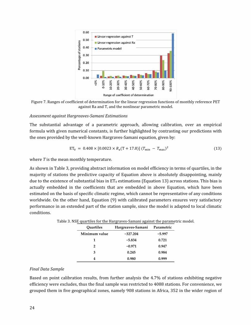
24
Figure 7. Ranges of coefficient of determination for the linear regression functions of monthly reference PET
against Ra and T, and the nonlinear parametric model.
Assessment against Hargreaves-Samani Estimations
The substantial advantage of a parametric approach, allowing calibration, over an empirical
formula with given numerical constants, is further highlighted by contrasting our predictions with
the ones provided by the well-known Hargraves-Samani equation, given by:
(13)
where T is the mean monthly temperature.
As shown in Table 3, providing abstract information on model efficiency in terms of quartiles, in the
majority of stations the predictive capacity of Equation above is absolutely disappointing, mainly
due to the existence of substantial bias in ET0 estimations (Equation 13) across stations. This bias is
actually embedded in the coefficients that are embedded in above Equation, which have been
estimated on the basis of specific climatic regime, which cannot be representative of any conditions
worldwide. On the other hand, Equation (9) with calibrated parameters ensures very satisfactory
performance in an extended part of the station sample, since the model is adapted to local climatic
conditions.
Table 3. NSE quartiles for the Hargraves-Samani against the parametric model.
Quartiles Hargreaves-Samani Parametric
Minimum value −327.204 −5.997
1 −5.834 0.721
2 −0.971 0.947
3 0.245 0.984
4 0.980 0.999
Final Data Sample
Based on point calibration results, from further analysis the 4.7% of stations exhibiting negative
efficiency were excludes, thus the final sample was restricted to 4088 stations. For convenience, we
grouped them in five geographical zones, namely 908 stations in Africa, 352 in the wider region of
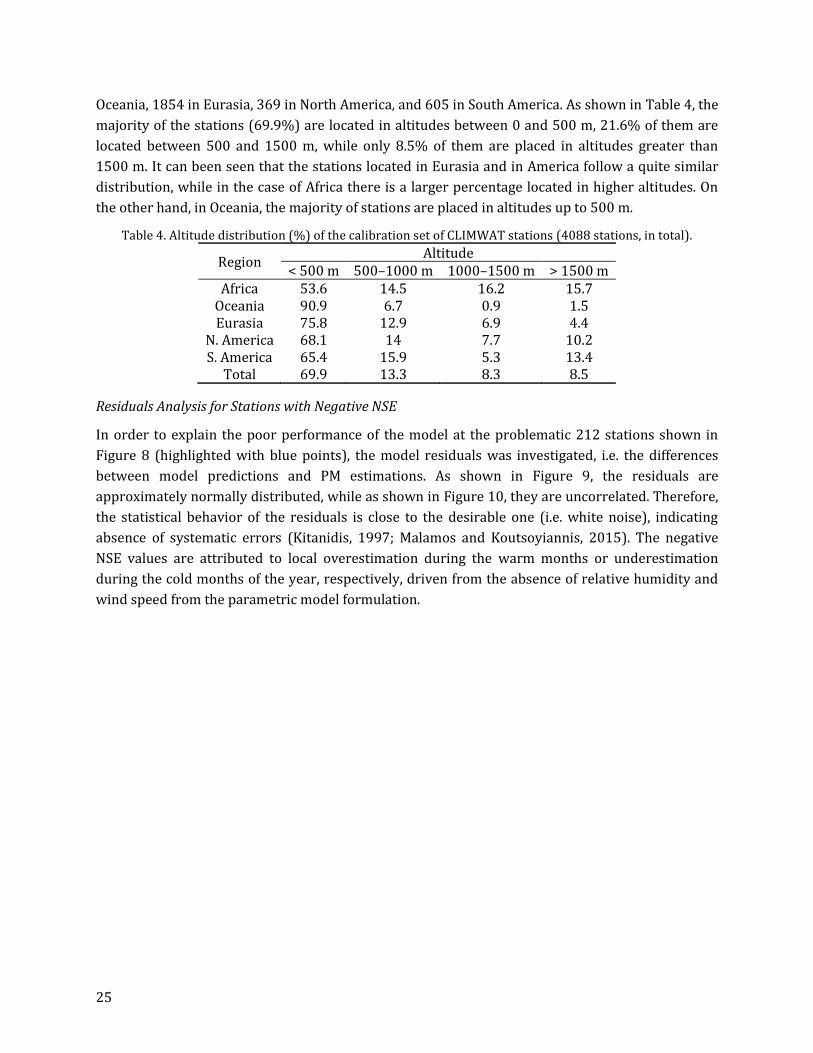
25
Oceania, 1854 in Eurasia, 369 in North America, and 605 in South America. As shown in Table 4, the
majority of the stations (69.9%) are located in altitudes between 0 and 500 m, 21.6% of them are
located between 500 and 1500 m, while only 8.5% of them are placed in altitudes greater than
1500 m. It can been seen that the stations located in Eurasia and in America follow a quite similar
distribution, while in the case of Africa there is a larger percentage located in higher altitudes. On
the other hand, in Oceania, the majority of stations are placed in altitudes up to 500 m.
Table 4. Altitude distribution (%) of the calibration set of CLIMWAT stations (4088 stations, in total).
Region Altitude
< 500 m 500–1000 m 1000–1500 m > 1500 m Africa 53.6 14.5 16.2 15.7
Oceania 90.9 6.7 0.9 1.5 Eurasia 75.8 12.9 6.9 4.4
N. America 68.1 14 7.7 10.2 S. America 65.4 15.9 5.3 13.4
Total 69.9 13.3 8.3 8.5
Residuals Analysis for Stations with Negative NSE
In order to explain the poor performance of the model at the problematic 212 stations shown in
Figure 8 (highlighted with blue points), the model residuals was investigated, i.e. the differences
between model predictions and PM estimations. As shown in Figure 9, the residuals are
approximately normally distributed, while as shown in Figure 10, they are uncorrelated. Therefore,
the statistical behavior of the residuals is close to the desirable one (i.e. white noise), indicating
absence of systematic errors (Kitanidis, 1997; Malamos and Koutsoyiannis, 2015). The negative
NSE values are attributed to local overestimation during the warm months or underestimation
during the cold months of the year, respectively, driven from the absence of relative humidity and
wind speed from the parametric model formulation.

26
Figure 8. CLIMWAT stations with negative NSE.

27
Figure 9. Normal probability plot of the empirical distribution function of the mode residuals using Weibull
plotting positions against normal distribution function N (0, 0.7), for stations with negative NSE.
Figure 10. Residuals vs parametric PET for stations with negative NSE.
In order to further evaluate the effect of missing information of relative humidity and wind speed
on the produced residuals, we plotted both of them along with the corresponding linear models, as
presented in Figure 11. This illustrates that there is a significant linear correlation between the
relative humidity and the estimation errors - residuals while the opposite seems to be the case for
the wind speed. The absence of these two variables as explanatory input variables within the
parametric model seem to be crucial in regions with seasonal variations of ET0 due to energy or
water limitations mainly in the tropical zone, as shown in Figure 8.

28
Figure 11. Residuals vs. humidity (a) and wind speed (b) for stations with negative NSE.
Evaluation of Model Performance across Geographical Zones
According to the acquired values of NSE (Table 5, Figure 12), the parametric model performs well
in Eurasia, North America, and the wider region of Oceania, where 80%, 80%, and 77% of stations,
respectively, present efficiency values more than 0.80. In South America, 66% of stations achieve a
score greater than 0.80, while in Africa, this percentage falls to 50%. In particular, 22% of stations
in Africa achieved NSE values below 0.50, which indicates a poor predictive capacity.
The mean absolute error of the parametric model in every geographical unit is small (Table 6). In
South America, the MAE of the 95% of the stations is below 4 mm/month. This percentage is 88%
for the wider region of Oceania, 79% for North America, 76% for Eurasia, and 72% for Africa.
Table 7 summarizes the values of the relative bias of the parametric model against the reference
PET values, for all of the geographical units (Figure 12). It is obvious that the values are generally
small, ranging from –0.122 to +0.062 proving that the results of the parametric model are almost
unbiased for the majority of the stations. The differences between the biases across the
geographical zones are not important, since the variation between the extreme values is similar.
The overall evaluation of the model across the different geographical areas is very satisfactory. All
of the metrics prove that the predictive capacity of the model is very satisfying across Eurasia,
North America, and the wider region of Oceania. On the other hand, in the equatorial regions of
South America, Africa as well as the Indian and Indonesian Peninsula (Figure 8), the model
performs poorly according to the NSE criterion, probably because it does not account for relative
humidity and wind speed, which are key drivers of the evapotranspiration processes across these
areas, influencing the net incoming solar radiation and the evaporation demand.

29
Table 5. Number of stations and associated NSE intervals across geographical zones.
Region 1.0–0.9 0.9–0.8 0.8–0.7 0.7–0.6 0.6–0.5 <0.5
Africa 34 16 12 9 7 22
Oceania 67 10 7 4 1 11
Eurasia 68 12 7 4 3 6
N. America 65 15 5 3 2 10
S. America 54 12 10 7 6 11
Table 6. Number of stations and associated intervals of monthly MAE across geographical zones.
Region 0–2 mm 2–4 mm 4–6 mm 6–8 mm 8–10 mm >10 mm
Africa 36 36 15 6 3 4
Oceania 52 36 9 3 0 0
Eurasia 39 37 17 5 1 1
N. America 40 39 17 3 1 0
S. America 69 26 4 1 0 0
Table 7. Number of stations and associated intervals of BIAS across geographical zones.
Region –0.122–0.000 0.000–0.001 0.001–0.062
Africa 65 14 21
Oceania 38 12 50
Eurasia 72 5 23
N. America 68 13 19
S. America 55 15 30

30
Figure 12. Distribution of NSE across CLIMWAT stations.

31
Figure 13. Distribution of BIAS across CLIMWAT stations.
32
Spatial Analysis and Model Validation
Spatial Interpolation of Optimized Parameters
Even though point PET estimates can be used for small-scale studies, it is the regionalisation of PET
that is of great significance in hydrological science (Merz and Blöschl, 2004). A preliminary attempt
in PET mapping was presented by Foyster (1973), and followed by several publications where
different spatial interpolation methods have been applied (Dalezios et al., 2002; Mardikis et al.,
2005; Vicente-Serrano et al., 2007), with satisfying performance. In a recent study, Tegos et al.
(2015) illustrated that the inverse distance method (IDW) was the most efficient than other
interpolation techniques, i.e. Kriging, Bilinear Surface Smoothing and Natural Neighbours.
Furthermore, IDW is a straightforward and computationally non-intensive method, which is
capable to address the huge spatial extent of the study area, i.e. the entire globe.
Formally, the IDW method is used to estimate the unknown value in location S0 given the
observed y values at sampled locations Si in the following manner:
(14)
Essentially, the estimated value in S0 is a linear combination of the weights (λi) and observed y
values in Si, where λi is defined as:
(15)
with:
(16)
In the above Equation, the numerator is the inverse of distance d0i between S0 and Si with a power α,
and the denominator is the sum of all inverse-distance weights for all locations i (in the particular
case, all stations exhibiting positive efficiency).
Spatial Distribution of Parameters
The approach allows for mapping the spatial distribution of the optimized model parameters a΄ and
c΄, instead of its response, i.e. PET. This is a major advantage, since it allows implementing Equation
(5) wherever in the globe, using interpolated values of the point (i.e., locally calibrated) parameters.
It is interesting to note that the two parameters are negatively correlated (Figure 14), thus
reflecting the significant correlation of the associated meteorological variables of the parametric
formula (extraterrestrial radiation, in the numerator, and temperature, in the denominator).
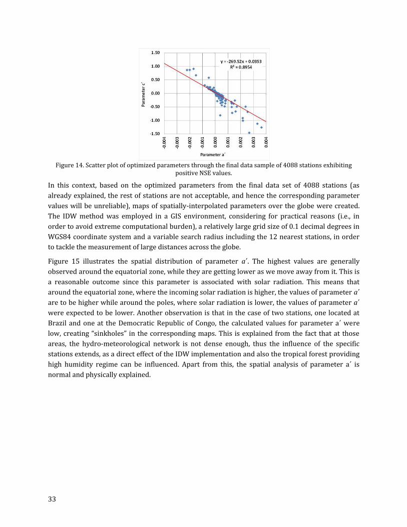
33
Figure 14. Scatter plot of optimized parameters through the final data sample of 4088 stations exhibiting
positive NSE values.
In this context, based on the optimized parameters from the final data set of 4088 stations (as
already explained, the rest of stations are not acceptable, and hence the corresponding parameter
values will be unreliable), maps of spatially-interpolated parameters over the globe were created.
The IDW method was employed in a GIS environment, considering for practical reasons (i.e., in
order to avoid extreme computational burden), a relatively large grid size of 0.1 decimal degrees in
WGS84 coordinate system and a variable search radius including the 12 nearest stations, in order
to tackle the measurement of large distances across the globe.
Figure 15 illustrates the spatial distribution of parameter a΄. The highest values are generally
observed around the equatorial zone, while they are getting lower as we move away from it. This is
a reasonable outcome since this parameter is associated with solar radiation. This means that
around the equatorial zone, where the incoming solar radiation is higher, the values of parameter a΄
are to be higher while around the poles, where solar radiation is lower, the values of parameter a΄
were expected to be lower. Another observation is that in the case of two stations, one located at
Brazil and one at the Democratic Republic of Congo, the calculated values for parameter a΄ were
low, creating “sinkholes” in the corresponding maps. This is explained from the fact that at those
areas, the hydro-meteorological network is not dense enough, thus the influence of the specific
stations extends, as a direct effect of the IDW implementation and also the tropical forest providing
high humidity regime can be influenced. Apart from this, the spatial analysis of parameter a΄ is
normal and physically explained.

34
Figure 15. Spatial distribution of parameter a΄ over the globe.
In contrast to parameter a΄, the spatial distribution of parameter c΄, depicted in Figure 16, the
lowest values around the equatorial zone, while these are getting higher as we move away from the
equator. Since c΄ is inversely proportional to temperature, it was expected that its values get higher
as temperature is getting lower and vice versa. In the case of the above stations, i.e. one at Brazil
and one at the Democratic Republic of Congo, the values of parameter c΄ were extremely high,
contrariwise to parameter a΄. The explanation for this phenomenon is the same as above, yet in this
case the interpolation method resulted in a ridge-type distribution over the specific areas.
Conclusively, the model results can be considered reliable, since the spatial distribution of both
parameters around the globe is physically explained, while minor irregularities are also attributed
to physical reasons, i.e. inadequate representation of humidity and wind processes.

35
Figure 16. Spatial distribution of parameter c΄ over the globe.
Model Validation
The validation of the model was performed by comparing monthly ET0 predictions provided by the
parametric formula using interpolated parameters against PM estimates in a number of
independent stations. In particular, two validations sets was considered, a “local” and a “global”
one. The former comprises 37 stations across California, for which monthly meteorological time
series are available from the California Irrigation Management Information System (Hart et al.,
2009). The “global” set comprises 17 stations from countries with different hydroclimatic regimes
(Spain, Germany, Ireland, Greece, Iran, and Australia), for which we obtained full time series of the
required meteorological data, at the monthly scale, form various data sources.
For the local validation set (Table 8), the model predicts monthly ET0 with significant accuracy, thus
exhibiting an average efficiency up to 0.855, and an average bias of only −0.07. Except for three
stations (Bishop, Castroville, De Laveaga), the NSE exceeds 0.70, while in 17 out of 37 stations it
exceeds 0.90. This indicates an almost perfect performance, particularly when taking into account
that the model has been calibrated using abstract (i.e. mean monthly) meteorological information
over the entire globe, while the validation set comprises detailed data, both in terms of spatial
extent and temporal resolution. Similarly satisfying are the outcomes from the global validation set,
which are summarized in Table 9 (average efficiency 0.852, average bias 0.02), thus confirming the
model predictive capacity across different climates.
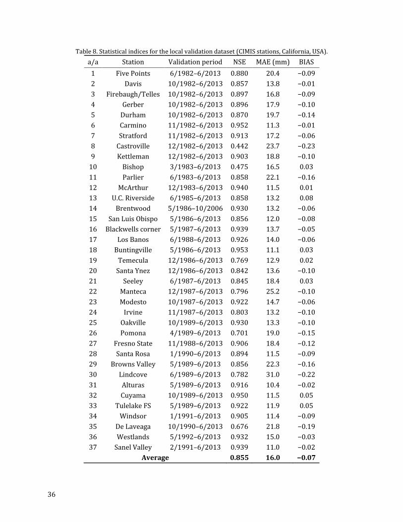
36
Table 8. Statistical indices for the local validation dataset (CIMIS stations, California, USA).
a/a Station Validation period NSE MAE (mm) BIAS
1 Five Points 6/1982–6/2013 0.880 20.4 −0.09
2 Davis 10/1982–6/2013 0.857 13.8 −0.01
3 Firebaugh/Telles 10/1982–6/2013 0.897 16.8 −0.09
4 Gerber 10/1982–6/2013 0.896 17.9 −0.10
5 Durham 10/1982–6/2013 0.870 19.7 −0.14
6 Carmino 11/1982–6/2013 0.952 11.3 −0.01
7 Stratford 11/1982–6/2013 0.913 17.2 −0.06
8 Castroville 12/1982–6/2013 0.442 23.7 −0.23
9 Kettleman 12/1982–6/2013 0.903 18.8 −0.10
10 Bishop 3/1983–6/2013 0.475 16.5 0.03
11 Parlier 6/1983–6/2013 0.858 22.1 −0.16
12 McArthur 12/1983–6/2013 0.940 11.5 0.01
13 U.C. Riverside 6/1985–6/2013 0.858 13.2 0.08
14 Brentwood 5/1986–10/2006 0.930 13.2 −0.06
15 San Luis Obispo 5/1986–6/2013 0.856 12.0 −0.08
16 Blackwells corner 5/1987–6/2013 0.939 13.7 −0.05
17 Los Banos 6/1988–6/2013 0.926 14.0 −0.06
18 Buntingville 5/1986–6/2013 0.953 11.1 0.03
19 Temecula 12/1986–6/2013 0.769 12.9 0.02
20 Santa Ynez 12/1986–6/2013 0.842 13.6 −0.10
21 Seeley 6/1987–6/2013 0.845 18.4 0.03
22 Manteca 12/1987–6/2013 0.796 25.2 −0.10
23 Modesto 10/1987–6/2013 0.922 14.7 −0.06
24 Irvine 11/1987–6/2013 0.803 13.2 −0.10
25 Oakville 10/1989–6/2013 0.930 13.3 −0.10
26 Pomona 4/1989–6/2013 0.701 19.0 −0.15
27 Fresno State 11/1988–6/2013 0.906 18.4 −0.12
28 Santa Rosa 1/1990–6/2013 0.894 11.5 −0.09
29 Browns Valley 5/1989–6/2013 0.856 22.3 −0.16
30 Lindcove 6/1989–6/2013 0.782 31.0 −0.22
31 Alturas 5/1989–6/2013 0.916 10.4 −0.02
32 Cuyama 10/1989–6/2013 0.950 11.5 0.05
33 Tulelake FS 5/1989–6/2013 0.922 11.9 0.05
34 Windsor 1/1991–6/2013 0.905 11.4 −0.09
35 De Laveaga 10/1990–6/2013 0.676 21.8 −0.19
36 Westlands 5/1992–6/2013 0.932 15.0 −0.03
37 Sanel Valley 2/1991–6/2013 0.939 11.0 −0.02
Average 0.855 16.0 −0.07

37
Table 9. Statistical indexes for the global validation dataset.
a/a Station Country Validation period NSE MAE (mm) BIAS
1 Aachen Germany 01/1951–5/2011 0.955 6.8 0.06
2 Bremen Germany 01/1951–5/2011 0.954 5.5 0.03
3 Alicante Spain 01/1980–09/2010 0.916 11.1 0.00
4 Badajoz Spain 01/1961–05/2005 0.921 13.0 −0.09
5 Valencia Spain 09/1954–08/1964 0.893 10.0 −0.06
6 Zaragoza Spain 02/1974–01/1996 0.953 10.8 −0.01
7 Herakleion Greece 01/1968–12/1989 0.947 10.2 −0.00
8 Kerkyra Greece 01/1968–12/1989 0.936 9.8 −0.09
9 Kavala Greece 01/1968–12/1989 0.835 13.5 0.04
10 Limnos Greece 01/1968–12/1989 0.762 24.3 0.12
11 Athens Greece 01/1968–12/1989 0.924 13.6 0.03
12 Melbourne Australia 01/2009–1/2016 0.752 18.5 0.17
13 Dublin Ireland 01/2013–6/2016 0.870 5.1 −0.09
14 Bandar-Anzali Iran 1/1990–12/2005 0.875 13.9 −0.16
15 Ramsar Iran 1/1990–12/2005 0.788 16.2 0.15
16 Khorram-Abad Iran 1/1990–12/2005 0.400 38.3 0.37
17 Kashan Iran 1/1990–12/2005 0.804 19.6 −0.13
Average 0.852 14.1 0.02
3.1.5 Conclusions
The concept of parametric PET modelling was thoroughly analyzed, by performing a global survey
of its applicability. The model has a very simple structure and uses easily retrieved information, by
means of air temperature and extraterrestrial radiation. Therefore, the model is simultaneously
simple and parsimonious, in terms of both parameterization and data requirements.
Preliminary analysis of the extended climatic data at 4300 stations worldwide, provided by the FAO
CLIMWAT database, allowed for justifying the use of temperature and extraterrestrial radiation as
key explanatory variables of reference PET over the globe. However, it also indicated that in few
cases the two variables exhibit irregular seasonal patterns, which cannot be adequately
represented through simple modelling structures. The statistical analysis of the residuals, in these
cases, showed that the model is consistent in terms of parameters estimation and model validation.
At all CLIMWAT stations, optimal estimations of model parameters c΄ and a΄ were provided, by
calibrating them against given Penman-Monteith values at the mean monthly scale. Using typical
goodness-of-fitting criteria (efficiency, mean absolute error, relative bias), the model performance
was evaluated, which was generally very satisfying in a large portion of stations. However, in less
than 10% of the data set the calibrated model exhibited negative efficiency. Further analysis across
broader geographical regions showed that the model deviates from the Penman-Monteith PET

38
estimates in some locations, which is rather expected due to the significant influence of relative
humidity and wind speed, which are not accounted for in the parametric model.
An important outcome of this research was the generation of spatially distributed maps of model
parameters, by employing the IDW interpolation technique against their optimized values at 4088
out of 4300 stations, exhibiting non-negative efficiency. The spatial pattern of both parameters
over the globe is fully reasonable, which is a strong indicator of their physical consistency. These
maps can be straightforwardly used to provide suitable parameter values at both the local and
regional scale, thus allowing for the direct use of the parametric model wherever in the world.
The validation procedure against PM estimates from detailed meteorological information (i.e.
monthly time series) from 37 stations across California, as well as 17 independent stations across
Europe, Asia, and Australia, proved that the application of the parametric model using spatially
interpolated parameters provides reliable estimates, thus being a promising alternative of the
widely recognized yet data demanding Penman-Monteith approach, when there is lack of the full
data set that the latter requires.

39
4 Parametric model in CIMIS network
4.1 Introduction
The following chapters present the development of the Parametric model in the CIMIS network
(California) along with some locals stations in Spain and Germany. The performance of the new
model was compared with well-established radiation-based (Hargreaves, Jensen-Haise, Mcguiness-
Bordne), temperature-based (Thorhwaite, Blaney Criddle) models. Finally, alternative spatial
techniques were applied for identifying the optimal interpretation of the spatial PET information.
4.2 Parametric formula
Parsimonious modeling is essential in several water discipline fields (Koutsoyiannis 2009,
Koutsoyiannis 2014). In this vein, the hydro model structure and the input should be easily
available. Due to highly complexity of the P-M equation, most of simplified formulas fail to describe
the phenomenon of evapotranspiration. Thus, the idea of replacing some variables and constants
used in the standard Penman-Monteith (PM) formula by a number of parameters which are
regionally varying and estimated through calibration from a reference evapotranspiration sample,
constitutes a new appealing strategy for evapotranspiration estimation.
Koutsoyiannis and Xanthopoulos (1999), Tegos et al. (2009) and Tegos et al. (2013) examined the
structure and the sensitivity of input data in PM model. They concluded that there is a direct
relationship between potential evapotranspiration, extraterrestrial radiation and temperature.
Furthermore, Mamassis et al. (2014) reached to the conclusion that the influence of every
meteorological parameter in evaporation is almost linear, with temperature having the greater
influence.
By dividing both the numerator and the denominator by Δ, the PM equation can be written in the
form:
PET = 1 ρ
Rn + γ F(u) D1 + γ' Δ (17)
In the above expression, the numerator is the sum of a term related to solar radiation and a term
related to the rest of meteorological variables, while the denominator is function of temperature.
Based on the previous analysis, a simplification of the Penman-Monteith formula, where the
numerator is approximated by a linear function of extraterrestrial solar radiation, while a linear
descending function of temperature approximates the denominator, can be described by the
following formula:
PET = a Ra b1 c Ta
(18)
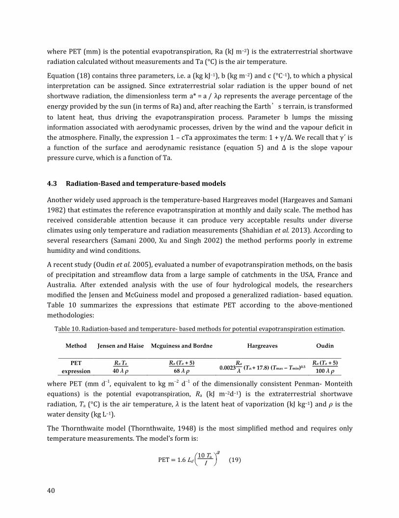
40
where PET (mm) is the potential evapotranspiration, Ra (kJ m–2) is the extraterrestrial shortwave
radiation calculated without measurements and Ta (°C) is the air temperature.
Equation (18) contains three parameters, i.e. a (kg kJ–1), b (kg m–2) and c (°C–1), to which a physical
interpretation can be assigned. Since extraterrestrial solar radiation is the upper bound of net
shortwave radiation, the dimensionless term a* = a / λρ represents the average percentage of the
energy provided by the sun (in terms of Ra) and, after reaching the Earth’s terrain, is transformed
to latent heat, thus driving the evapotranspiration process. Parameter b lumps the missing
information associated with aerodynamic processes, driven by the wind and the vapour deficit in
the atmosphere. Finally, the expression 1 – cTa approximates the term: 1 + γ/Δ. We recall that γ΄ is
a function of the surface and aerodynamic resistance (equation 5) and Δ is the slope vapour
pressure curve, which is a function of Ta.
4.3 Radiation-Based and temperature-based models
Another widely used approach is the temperature-based Hargreaves model (Hargeaves and Samani
1982) that estimates the reference evapotranspiration at monthly and daily scale. The method has
received considerable attention because it can produce very acceptable results under diverse
climates using only temperature and radiation measurements (Shahidian et al. 2013). According to
several researchers (Samani 2000, Xu and Singh 2002) the method performs poorly in extreme
humidity and wind conditions.
A recent study (Oudin et al. 2005), evaluated a number of evapotranspiration methods, on the basis
of precipitation and streamflow data from a large sample of catchments in the USA, France and
Australia. After extended analysis with the use of four hydrological models, the researchers
modified the Jensen and McGuiness model and proposed a generalized radiation- based equation.
Table 10 summarizes the expressions that estimate PET according to the above-mentioned
methodologies:
Table 10. Radiation-based and temperature- based methods for potential evapotranspiration estimation.
Method Jensen and Haise Mcguiness and Bordne Hargreaves Oudin
PET
expression
Ra Ta
40 λ ρ
Ra (Ta + 5)
68 λ ρ 0.0023
Ra
λ (Tα + 17.8) (Tmax – Tmin)0.5
Ra (Ta + 5)
100 λ ρ
where PET (mm d–1, equivalent to kg m–2 d–1 of the dimensionally consistent Penman- Monteith
equations) is the potential evapotranspiration, Ra (kJ m–2d–1) is the extraterrestrial shortwave
radiation, Ta (°C) is the air temperature, λ is the latent heat of vaporization (kJ kg–1) and ρ is the
water density (kg L–1).
The Thornthwaite model (Thornthwaite, 1948) is the most simplified method and requires only
temperature measurements. The model’s form is:
PET = 1.6 Ld
10 Ta
I
a (19)
41
where PET is the potential evapotranspiration (mm/month), Ld is the daytime length, Ta is the mean
monthly air temperature (oC), I is the annual heat index and a is an empirically determined
parameter which is function of I.
The temperature-based Blaney-Criddle method (Blaney and Criddle, 1962) has received worldwide
application for the estimation of irrigation demands. The model expression is:
(20)
where PET is the potential evapotranspiration (mm/month), Ta the mean temperature (oC), K is the
monthly consumptive use coefficient and p is the mean daily percentage of annual daytime hours.
4.4 Hydrometeorological data and computational tools
For exploration purposes, monthly meteorological data from 39 CIMIS stations were used, available
at www.cimis.water.ca.gov, 10 stations from Germany and finally 4 stations from Spain (Table 11).
The European data are freely available in the European Climate Assessment dataset
(http://eca.knmi.nl/). Stations latitudes range from N 32.76o to N 53.38o and their altitude varies
from 2.74 m to 1342.6 m.
The available data comprise mean temperature, relative humidity, sunshine duration and wind
velocity. At all CIMIS stations the data covers the period from October 1992 to September 2012
while the European stations cover the period from January 1948 to December 2013. The choice of
the time-periods was based on the simultaneous availability of the four required
hydrometeorological variables (temperature, sunshine duration, humidity, wind speed).
Additionally, the selection of each station and especially those from the CIMIS network was based
on the existence of adequate length time series for the processes involved, i.e. 20 years.
Table 11. Meteorological stations used for the evaluation of the potential evapotranspiration methods

42
The time series processing along for the implementation of the different approaches for potential
evapotranspiration estimation, i.e. Penman-Monteith, parametric and Hargreaves, was carried out
using the free software application Hydrognomon (Kozanis et al. 2010, http://hydrognomon.org/),
while the remaining expressions (Jensen, McGuiness and Oudin) were evaluated through
spreadsheets.
4.5 Statistical criteria
The main statistical criterion used for the evaluation of the methodologies performance against the
values computed by the Penman Monteith method (PM) was the coefficient of efficiency (CE),
introduced by Nash & Sutcliffe (1970):
CE = 1
i=1
n( )PEi PMi
2
i=1
n
(PM
PMi)2
(21)
Νο. Station name, Location Νο. Station name, Location Νο. Station name, Location
1 Five Points, U.S.A. 19 Buntigville, U.S.A. 37 De Laveaga, U.S.A.
2 Davis, U.S.A. 20 Temecula, U.S.A. 38 Westlands, U.S.A.
3 Firebaugh Teles, U.S.A. 21 Santa Ynez, U.S.A. 39 Sanel Valley, U.S.A.
4 Gerber, U.S.A. 22 Seeley, U.S.A. 40 Aachen, Germany
5 Durham, U.S.A. 23 Manteca, U.S.A. 41 Angermunde, Germany
6 Carmino, U.S.A. 24 Modesto, U.S.A. 42 Bremen-Seefahrtshule,
Germany
7 Stratford, U.S.A. 25 Irvine, U.S.A. 43 Dresden-Klotzsche,
Germany
8 Castorville, U.S.A. 26 Oakville, U.S.A. 44 Dusseldorf, Germany
9 Kettleman, U.S.A. 27 Pomona, U.S.A. 45 Frankfurt, Germany
10 Bishop, U.S.A. 28 Frenso State, U.S.A. 46 Hamburg Fuhlsbuettel,
Germany
11 Parlier, U.S.A. 29 Santa Rosa, U.S.A. 47 Karlsrhue, Germany
12 Calipatria, U.S.A. 30 Browns Valley, U.S.A. 48 Muenchen-Flughafen,
Germany
13 Mc Arthur, U.S.A. 31 Lindcove, U.S.A. 49 Stuggart-Schnarreberg,
Germany
14 UC Riverside, U.S.A. 32 Meloland, U.S.A. 50 Alicante, Spain
15 Brentwood, U.S.A. 33 Alturas, U.S.A. 51 Badajoz Televera, Spain
16 San Luis Obispo, U.S.A. 34 Cuyama, U.S.A. 52 Valencia, Spain
17 Blackwells Corner, U.S.A. 35 Tulelake, U.S.A. 53 Zaragoza Aeropuerto,
Spain
18 Los Banos, U.S.A. 36 Windsor, U.S.A.

43
where PMi and PEi are the potential evapotranspiration values of month i, computed by the
Penman-Monteith method and the other model respectively, PM––– is the monthly average over the
common data period estimated by the Penman-Monteith formula while n is the sample size.
Additionally, we applied several statistical measures, such as the mean bias error:
MBE = 1n
i=1
n( )PEi PMi (22)
the mean average error: MAE = 1n
i=1
n |PEi PMi| (23)
and the root mean square error: RMSE =
1n
i=1
n
(PEi PMi)2
1/2
(24)
CE ranges between −∞ and 1 (1 inclusive), with CE = 1 being the optimal value. Values between 0
and 1 are generally regarded as acceptable levels of performance, whereas values less than 0
indicate that the mean observed value is a better predictor than the simulated value, which
indicates unacceptable performance. MBE, MAE and RMSE values of 0 indicate a perfect fit (Moriasi
et al. 2007).
4.6 Results
The implementation of the parametric model was accomplished by calculating the three
parameters involved at each station, as mentioned above. This procedure is automated via a least
square optimization technique, embedded in the Hydrognomon software (Kozanis et al. 2010,
http://hydrognomon.org/), providing means for acquiring optimized values of a, b and c
parameters for the parametric method application.
The calculated monthly Penman-Monteith potential evapotranspiration time series acted as the
reference data sets against which the comparisons between the different methodologies took place.
Table 12 summarizes the values of the parameters for each of the 53 stations, acquired by the
procedure described above.

44
Table 12: Meteorological stations numbers and corresponding parameter values for the parametric method
4.7 Comparison with radiation-based methods
Figure 17 presents the mean annual potential evapotranspiration calculated by the Penman-
Monteith method for each one of the 39 CIMIS stations against the parametric and the other four
methods. It is clear that the parametric, Hargreaves and McGuiness models respect the variation of
Station a b c Station a b c
Νο. (kg kJ–1
) (kg m–2
) (°C–1
) Νο. (kg kJ–1
) (kg m–2
) (°C–1
)
1 1.47 10–4
1.49 1.58 10–2
28 1.29 10–4
1.3 1.73 10–2
2 1.04 10–4
6.51 10–1
2.15 10–2
29 8.88 10–5
6.09 10–1
2.63 10–2
3 1.46 10–4
1.48 1.47 10–2
30 8.95 10–5
4.07 10–1
2.11 10–2
4 1.02 10–4
4.97 10–1
1.93 10–2
31 1.12 10–4
1.04 1.74 10–2
5 1.97 10–4
2.07 –2.70 10–4
32 2.12 10–4
2 4.94 10–3
6 8.82 10–5
2.49 10–1
2.34 10–2
33 7.92 10–5
–2.20 10–1
2.44 10–2
7 1.12 10–4
–2.50 10–1
1.44 10–2
34 1.08 10–4
4.03 10–1
1.97 10–2
8 1.68 10–4
1.06 –3.60 10–2
35 9.28 10–5
5.20 10–2
2.12 10–2
9 1.34 10–4
1.23 1.62 10–2
36 8.65 10–5
5.66 10–1
2.60 10–2
10 1.43 10–4
7.39 10–1
1.05 10–2
37 1.02 10–4
5.82 10–1
1.24 10–2
11 1.29 10–4
1.32 1.61 10–2
38 1.40 10–4
1.33 1.67 10–2
12 1.69 10–4
1.32 8.86 10–3
39 9.88 10–5
6.54 10–1
2.37 10–2
13 9.75 10–5
4.26 10–1
2.36 10–2
40 3.96 10–5
–2.46 10–1
2.62 10–2
14 8.68 10–5
5.10 10–2
1.78 10–2
41 3.96 10–5
–2.58 10–1
2.73 10–2
15 1.11 10–4
9.00 10–1
2.09 10–2
42 4.28 10–5
–1.64 10–1
2.68 10–2
16 8.10 10–5
1.60 10–1
2.28 10–2
43 3.67 10–5
–3.45 10–1
2.81 10–2
17 1.21 10–4
1.02 1.89 10–2
44 4.12 10–5
–3.02 10–1
2.64 10–2
18 1.31 10–4
1.31 1.81 10–2
45 4.75 10–5
–8.8 10–2
2.62 10–2
19 9.29 10–5
–1.10 10–1
2.11 10–2
46 4.18 10–5
–1.66 10–1
2.66 10–2
20 6.66 10–5
–2.80 10–1
2.10 10–2
47 4.64 10–5
–6.6 10–2
2.58 10–2
21 9.44 10–5
4.91 10–1
2.06 10–2
48 4.69 10–5
–8.8 10–2
2.51 10–2
22 2.50 10–4
2.58 7.52 10–4
49 4.53 10–5
–1.64 10–1
2.52 10–2
23 1.13 10–4
1.02 2.03 10–2
50 5.89 10–5
–4.67 10–1
1.84 10–2
24 1.17 10–4
1.08 2.00 10–2
51 6.24 10–5
1.72 10–1
2.35 10–2
25 6.64 10–5
–4.40 10–2
2.28 10–2
52 5.34 10–5
–1.93 10–1
1.96 10–2
26 8.42 10–5
4.29 10–1
2.54 10–2
53 7.00 10–5
–2.2 10–2
2.39 10–2
27 1.13 10–4
1.25 2.00 10–2

45
the over-annual potential evapotranspiration, while the other two models, i.e. Oudin and Jensen-
Haise underestimate and overestimate respectively, the potential evapotranspiration values.
Figure 17. Mean annual Penman-Monteith potential evapotranspiration (symbols) for the 39 CIMIS stations against the parametric model and the other four methods
The performance indices presented in Table 13 confirm the good performance of the parametric
method, which has the highest CE and excellent results in the other statistical indices. The
Hargreaves model follows with CE 78.9%, similar MBE and worst MAE and RMSE than the
parametric model. The McGuiness method gave moderate results, while the Jensen-Haise and Oudin
models totally fail to represent the physical flux.
Table 13 Values of performance indices used to evaluate the parametric method, in the estimation of mean annual potential evapotranspiration for the 39 CIMIS stations, against the other four models
For further comparison of the parametric method against the four radiation-based methods, in
terms of the achieved CE distribution from estimating monthly PE, each time series was split into
two parts. The first 13 years were used as the calibration data set for the parametric model, while
the remaining 7 years were used for validation. Table 14 presents the CE distribution, for the
500
800
1100
1400
1700
2000
2300
2600
1 3 5 7 9 11 13 15 17 19 21 23 25 27 29 31 33 35 37 39
Mea
n a
nn
ua
l PE
(m
m)
Station number
Penman-Monteith Jensen-Haise
Parametric Mcguiness
Hargreaves Oudin
Method CE
(%)
MBE
(mm)
MAE
(mm)
RMSE
(mm)
Parametric 99.1 4 6 17
Hargreaves 78.9 2 60 82
Jensen-Haise < 0 417 452 493
McGuiness 30.1 19 111 149
Oudin < 0 -393 393 411
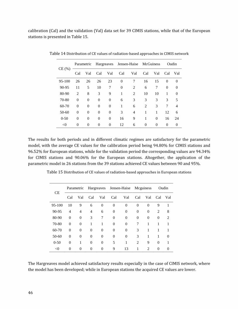
46
calibration (Cal) and the validation (Val) data set for 39 CIMIS stations, while that of the European
stations is presented in Table 15.
Table 14 Distribution of CE values of radiation-based approaches in CIMIS network
The results for both periods and in different climatic regimes are satisfactory for the parametric
model, with the average CE values for the calibration period being 94.80% for CIMIS stations and
96.52% for European stations, while for the validation period the corresponding values are 94.34%
for CIMIS stations and 90.06% for the European stations. Altogether, the application of the
parametric model in 26 stations from the 39 stations achieved CE values between 90 and 95%.
Table 15 Distribution of CE values of radiation-based approaches in European stations
The Hargreaves model achieved satisfactory results especially in the case of CIMIS network, where
the model has been developed; while in European stations the acquired CE values are lower.
CE (%)
Parametric Hargreaves Jensen-Haise McGuiness Oudin
Cal Val Cal Val Cal Val Cal Val Cal Val
95-100 26 26 26 23 0 7 16 15 0 0
90-95 11 5 10 7 0 2 6 7 0 0
80-90 2 8 3 9 1 2 10 10 1 0
70-80 0 0 0 0 6 3 3 3 3 5
60-70 0 0 0 0 1 6 2 3 7 4
50-60 0 0 0 0 3 4 1 1 12 6
0-50 0 0 0 0 16 9 1 0 16 24
<0 0 0 0 0 12 6 0 0 0 0
CE
Parametric Hargreaves Jensen-Haise Mcguiness Oudin
Cal Val Cal Val Cal Val Cal Val Cal Val
95-100 10 9 6 0 0 0 0 0 9 1
90-95 4 4 4 6 0 0 0 0 2 8
80-90 0 0 3 7 0 0 0 0 0 2
70-80 0 0 1 1 0 0 7 1 1 1
60-70 0 0 0 0 0 0 3 1 1 1
50-60 0 0 0 0 0 0 3 1 1 0
0-50 0 1 0 0 5 1 2 9 0 1
<0 0 0 0 0 9 13 1 2 0 0
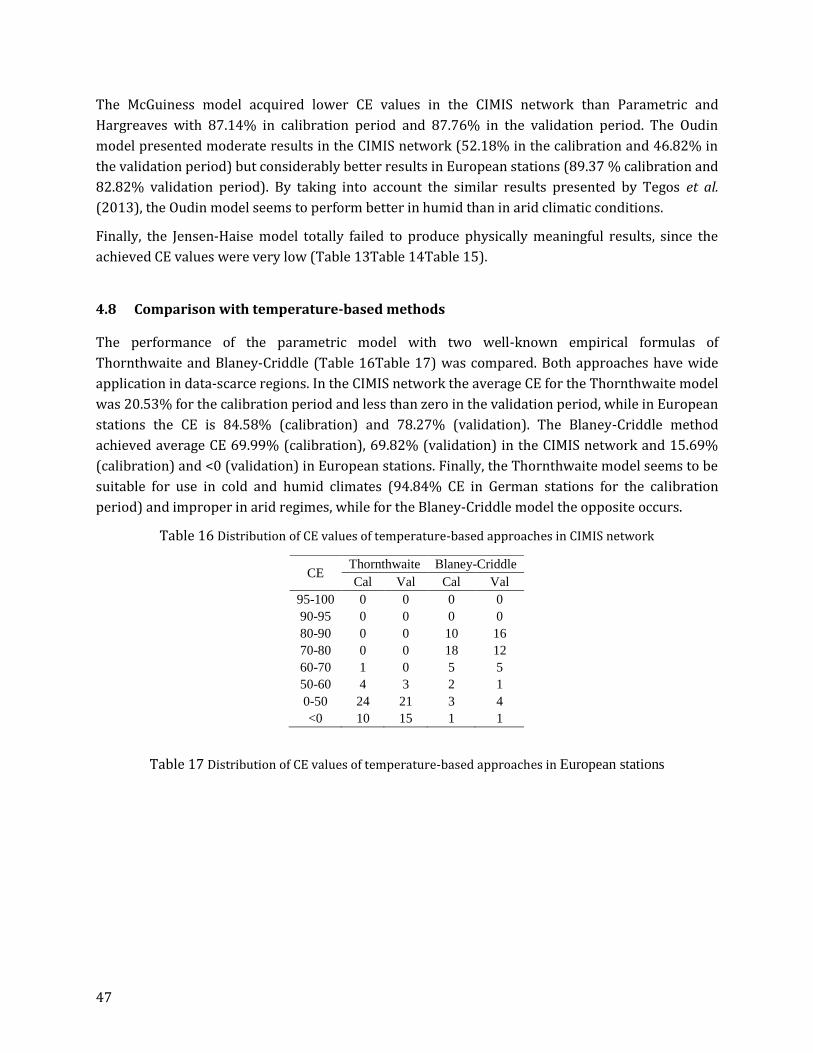
47
The McGuiness model acquired lower CE values in the CIMIS network than Parametric and
Hargreaves with 87.14% in calibration period and 87.76% in the validation period. The Oudin
model presented moderate results in the CIMIS network (52.18% in the calibration and 46.82% in
the validation period) but considerably better results in European stations (89.37 % calibration and
82.82% validation period). By taking into account the similar results presented by Tegos et al.
(2013), the Oudin model seems to perform better in humid than in arid climatic conditions.
Finally, the Jensen-Haise model totally failed to produce physically meaningful results, since the
achieved CE values were very low (Table 13Table 14Table 15).
4.8 Comparison with temperature-based methods
The performance of the parametric model with two well-known empirical formulas of
Thornthwaite and Blaney-Criddle (Table 16Table 17) was compared. Both approaches have wide
application in data-scarce regions. In the CIMIS network the average CE for the Thornthwaite model
was 20.53% for the calibration period and less than zero in the validation period, while in European
stations the CE is 84.58% (calibration) and 78.27% (validation). The Blaney-Criddle method
achieved average CE 69.99% (calibration), 69.82% (validation) in the CIMIS network and 15.69%
(calibration) and <0 (validation) in European stations. Finally, the Thornthwaite model seems to be
suitable for use in cold and humid climates (94.84% CE in German stations for the calibration
period) and improper in arid regimes, while for the Blaney-Criddle model the opposite occurs.
Table 16 Distribution of CE values of temperature-based approaches in CIMIS network
Table 17 Distribution of CE values of temperature-based approaches in European stations
CE Thornthwaite Blaney-Criddle
Cal Val Cal Val
95-100 0 0 0 0
90-95 0 0 0 0
80-90 0 0 10 16
70-80 0 0 18 12
60-70 1 0 5 5
50-60 4 3 2 1
0-50 24 21 3 4
<0 10 15 1 1

48
4.9 Spatial analysis of the parameters
The knowledge of the spatial variability of the PET is crucial in geosciences and the use of the
appropriate interpolation technique significant (Mancosu et al. 2014) The key idea of the
parametric model is the replacement of some of the variables and constants that are used in
standardized Penman-Monteith formula by three parameters, which are regionally varying and
estimated through calibration using a reference evapotranspiration data set.
In this context, two applications are implemented. The first is the analysis of the parameters’
correlation to latitude and elevation, while the second is their estimation, through spatial
interpolation techniques, along an extensive study area such as California, which provides sufficient
data to perform the necessary calibration procedures.
4.10 Correlation to latitude and elevation
Through regression analysis, the correlation of every parameter (a, b, c) with latitude φ and
elevation was investigated. Six scatter plots of Figure 18 show that parameters a, b are negatively
correlated to latitude and elevation, in contrast to parameter c. This is similar to the findings of the
previous study over the Greek territory (Tegos et al. 2013) for parameter a. It also appears a
noticeable correlation of parameter b with elevation (R = –0.50) and insignificant correlation of
parameter c with elevation and latitude. Furthermore, Figure 18 shows that the relation of the
three parameters to latitude and elevation is far from linear.
CE Thornthwaite Blaney-Criddle
Cal Val Cal Val
95-100 5 0 0 0
90-95 5 1 0 0
80-90 0 9 0 0
70-80 2 1 1 1
60-70 0 1 0 0
50-60 1 1 0 1
0-50 1 1 12 1
<0 0 0 1 11

49
Figure 18. Scatter plots of parameters against latitude and elevation
4.11 Spatial interpolation over California
Currently, a lot of methods exist which can accomplish spatial interpolation using available
computer codes. In the present study, the three parameters’ spatial variability was investigated by
R² = 0.06
-0.04
-0.03
-0.02
-0.01
0
0.01
0.02
0.03
32 34 36 38 40 42
Par
amet
er c
(o C−
1 )
Station latitude (o)
R² = 0.05
-0.04
-0.03
-0.02
-0.01
0
0.01
0.02
0.03
0 450 900 1350
Par
amet
er c
(oC
−1)
Station elevation (m)
R² = 0.10
-0.5
0
0.5
1
1.5
2
2.5
3
32 34 36 38 40 42
Par
amet
er b
(kgr
/m−
2 d−
1 )
Station latitude (o)
R² = 0.24
-0.5
0
0.5
1
1.5
2
2.5
3
0 450 900 1350
Par
amet
er b
(kgr
/m−
2 d−
1 )
Station elevation (m)
R² = 0.12
4.5E-05
9.5E-05
1.5E-04
2.0E-04
2.5E-04
3.0E-04
32 34 36 38 40 42
Par
amet
er a
(kg/
kJ)
Station latitude (o)
R² = 0.09
4.5E-05
9.5E-05
1.5E-04
2.0E-04
2.5E-04
3.0E-04
0 450 900 1350
Par
amet
er a
(kg/
kJ)
Station elevation (m)

50
four different methodologies: (1) Inverse Distance Weighting (IDW); (2) Natural Neighbours (NaN);
(3) Ordinary Kriging (OK); and (4) Bilinear Surface Smoothing (BSS)
The first three are well established and commonly used in spatial interpolation of environmental
variables (Li and Heap, 2008). The Bilinear Surface Smoothing methodology is a new approach that
approximates a surface that may be drawn for the data points with consecutive bilinear surfaces
which can be numerically estimated by means of a least squares fitting procedure into a surface
regression model with known break points and adjustable weights defined by means of angles
formed by those bilinear surfaces. The BSS theory and basic features are presented in Malamos and
Koutsoyiannis (2015) while applications and field validation are presented in Malamos and
Koutsoyiannis (2015) . BSS is implemented by means of a dynamic link library in Object Pascal
(Delphi) programming language linked to MS-Excel. The parameter estimation is based on the
generalized cross-validation methodology as described in Malamos and Koutsoyiannis (2015-a).
The obtained optimal values of the four adjustable parameters: the number of intervals according
to x and y directions, i.e. mx, my and the corresponding smoothing parameters τλx and τλy, are
presented in Table 18:
Table 18 BSS parameters optimal values for the CIMIS network (California area)
IDW and NaN were implemented in ESRI’s ArcGIS environment using the default settings, while for
OK all semivariogram models available in that software were investigated, i.e. circular, exponential,
spherical, linear and Gaussian,. In every case, the embedded fitting procedure ensured the
minimization of the weighted sum of squares between experimental and model semivariogram
values.
Table 19 presents the values of the statistical criteria for each one of the implemented
semivariogram models, sorted according to the CE criterion for each of the three parameters. It is
obvious that the circular semivariogram achieved the best overall performance.
Table 19 Values of the statistical criteria used to assess the performance of the different kriging semivariogram models
Parameter mx my τλx τλy
a
(kg kJ–1
) 3 8 0.082 0.001
b
(kg m–2
) 3 28 0.001 0.01
c
(°C–1
) 3 8 0.001 0.001

51
All three parameters of the parametric model were estimated over California by applying the four
spatial interpolation methods. The input data set consists of the calculated parameters values at the
39 CIMIS stations (Figure 19, Table 3).
Parameter kriging
semivariogram CE (%) MBE MAE RMSE
a
(kg kJ–1
)
circular 99.9 1.03 10–8
5.18 10–7
8.93 10–7
exponential 99.9 1.03 10–8
5.18 10–7
8.93 10–7
linear 99.9 1.03 10–8
5.18 10–7
8.93 10–7
spherical 99.9 1.03 10–8
5.18 10–7
8.93 10–7
gaussian 44.6 1.24 10–6
1.86 10–5
2.88 10–5
b
(kg m–2
)
exponential 72.8 3.12 10–3
2.50 10–1
3.43 10–1
circular 68.6 4.24 10–3
2.71 10–1
3.68 10–1
spherical 67.4 5.46 10–3
2.77 10–1
3.76 10–1
linear 66.6 6.00 10–3
2.81 10–1
3.80 10–1
gaussian 29.7 4.09 10–2
4.07 10–1
5.51 10–1
c
(°C–1
)
circular 39.3 3.56 10–4
4.62 10–3
8.19 10–3
spherical 11.7 4.64 10–4
5.60 10–3
9.88 10–3
exponential 11.0 4.67 10–4
5.62 10–3
9.92 10–3
linear 11.0 4.67 10–4
5.62 10–3
9.92 10–3
gaussian 11.0 4.67 10–4
5.62 10–3
9.92 10–3

52
Figure 19 Study area and the CIMIS Stations used for spatial analysis
Table 20 presents the values of the statistical criteria used to assess the performance of the spatial
interpolation methods with respect to the input data set. It is apparent that both non-geostatistical
methods, according to the statistical criteria used, outperform ordinary kriging and bilinear surface
smoothing, which performed similarly. This is not a surprise because both IDW and NaN, from
construction, use as best local predictor the available data points (Li and Heap, 2008).
Table 20 Values of the statistical criteria used to assess the performance of the spatial interpolation methods
with respect to the input data set
However, the above statistical indices may not be representative with respect to the validity of the
interpolation results in other locations, except for those incorporated in the interpolation
procedure. In this context, a validation procedure was implemented by means of comparing the
reference potential evapotranspiration estimates acquired from the implementation of the
parametric method, using the parameter estimates of the four interpolation methods, against those
of the eleven additional CIMIS stations with adequate time series length, shown in Table 21 along
with the estimated parameter values, in the case of IDW.
Parameter Interpolation
Method CE (%) MBE MAE RMSE
a
(kg kJ–1
)
IDW 100 3.59 10–8
1.08 10–7
1.97 10–7
NaN 100 –1.03 10–7
4.77 10–7
8.95 10–7
OK 99.9 1.03 10–8
5.18 10–7
8.93 10–7
BSS 73.2 4.36 10–8
1.35 10–5
2.01 10–5
b
(kg m–2
)
IDW 100 2.95 10–4
1.72 10–3
3.06 10–3
NaN 99.9 –9.48 10–4
1.16 10–2
2.12 10–2
OK 68.6 4.24 10–3
2.71 10–1
3.68 10–1
BSS 65.2 1.97 10–4
2.68 10–1
3.88 10–1
c
(°C–1
)
IDW 100 2.56 10–7
8.82 10–6
1.52 10–5
NaN 99.9 1.54 10–6
1.50 10–4
3.10 10–4
OK 39.3 3.56 10–4
4.62 10–3
8.19 10–3
BSS 68.9 –2.57 10–7
3.25 10–3
5.87 10–3

53
Table 21 CIMIS Stations used for validation purposes and estimated parameters values in the case of IDW
The performance of each method is presented in Table 22, which summarizes the CE values
acquired from the validation procedure. It is apparent that IDW outperforms the other three
methods in the majority of the cases. This is an interesting fact, since the IDW method is the
effortless of the four methodologies. On the other hand, the BSS performance is analogous or better
to that of the input data setdata set. NaN and OK performed similarly, with the first achieving
slightly superior outcome, since OK in the case of Borrego Springs resulted in negative CE value.
Table 22 CE values for every interpolation method in validation procedure stations
The variation of the three parameters over California produced by the IDW technique is illustrated
in Figure 20. It is apparent that both a and c present an increasing North to South gradient, while
Station a
(kg kJ–1
)
b
(kg m–2
)
c
(°C–1
)
Arroyo Seco 1.38 10–4
1.06 1.20 10–3
Carneros 9.10 10–5
5.48 10–1
2.42 10–2
Green Valey Road 1.16 10–4
7.75 10–1
7.26 10–3
King City Oasis 1.34 10–4
1.09 9.53 10–3
Santa Barbara 1.03 10–4
5.56 10–1
1.98 10–2
Alpaugh 1.23 10–4
8.27 10–1
1.67 10–2
Auburn 1.04 10–4
6.20 10–1
1.99 10–2
Borrego Springs 1.73 10–4
1.44 9.33 10–3
Lodi West 1.10 10–4
8.54 10–1
2.05 10–2
Merced 1.30 10–4
1.20 1.73 10–2
Palmdale 1.01 10–4
7.86 10–1
2.00 10–2
Station IDW NaN OK BSS
Arroyo Seco 77.7 78.9* 76.8 66.8
Carneros 96.1 96.2* 83.6 95.9
Green Valey Road 71.6* 69.5 70.2 65.7
King City Oasis 85.1 60.3 93.6* 64.3
Santa Barbara 47.9 72.4 78.2* 23.4
Alpaugh 95.7 95.5 96.0* 95.9
Auburn 94.4* 93.6 94.3 85.8
Borrego Springs 85.3* 81.3 <0 70.1
Lodi West 94.0* 93.7 92.9 92.3
Merced 96.9 97.1* 96.9 89.5
Palmdale 69.6 70.3 91.1* 56.0
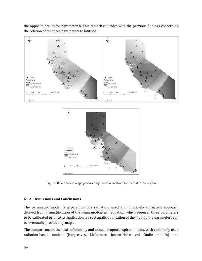
54
the opposite occurs for parameter b. This remark coincides with the previous findings concerning
the relation of the three parameters to latitude.
Figure 20 Parameters maps produced by the IDW method, for the California region
4.12 Discussions and Conclusions
The parametric model is a parsimonious radiation-based and physically consistent approach
derived from a simplification of the Penman-Monteith equation, which requires three parameters
to be calibrated prior to its application. By systematic application of the method the parameters can
be eventually provided by maps.
The comparison, on the basis of monthly and annual evapotranspiration data, with commonly used
radiation-based models (Hargreaves, McGuiness, Jensen-Haise and Oudin models) and

55
temperature-based models (Thorthwaite and Blaney-Criddle), verified the parametric model’s high
efficiency in different climatic regimes.
A parameters analysis, through regression techniques, was conducted in order to investigate their
correlation to latitude and elevation variation. Moreover, the parameters’ spatial estimation was
accomplished by implementing interpolation techniques such as: Inverse Distance Weighting
(IDW), Natural Neighbours (NaN), Ordinary Kriging (OK) and Bilinear Surface Smoothing (BSS),
along an extensive study area such as California. The validation procedure was implemented by
comparing the reference potential evapotranspiration estimates acquired from the implementation
of the parametric method, using the parameter estimates of the four interpolation methods, against
those of the eleven additional CIMIS stations. This combined evaluation of the four different
interpolation approaches, indicated that the simple and effortless IDW method performs better
than the other three methodologies. Regarding the application of the new methodology, BSS’s
efficiency to perform interpolation between data points that are interrelated in a complicated
manner was confirmed, acquiring high CE values analogous to those of the other three methods.
Overall, the key idea of the parametric model methodology, which is the simplification of the
Penman-Monteith formula by introducing three parameters, which are regionally varying and
estimated through calibration using a reference evapotranspiration data set, was very successful.

56
5 Global PET maps based on monthly remote temperatures
5.1 Introduction
Evapotranspiration (ET) is a crucial element of the hydrological cycle affecting a wide range of
geosciences, since it is referred as the combined water losses from soil surface and vegetation
influence by several meteorological variables such as the air temperature, the solar radiation, the
wind speed and the relative humidity. The literature proposes several approaches to quantify the
process in terms of actual evapotranspiration, potential evapotranspiration (PET) or reference
evapotranspiration. By definition the PET refers to “the rate at which evapotranspiration would
occur from a large area completely and uniformly covered with growing vegetation, which has
access to an unlimited supply of soil water, and without advection or heating effects” (Dingman,
1994), and differs to Actual Evatranspiration based on the soil water supply mainly driven by the
precipitation regime.In the last decades advanced methods were introduced for the ET and PET
estimation with the most recent being the remote sensing techniques incorporating aerial and
satellite imagery. Generally, the classification of the remote sensing for ET assessment includes four
groups referred to as empirical, direct, residual, inference and deterministic models (Nouri et al.,
2013). The most well-known approach for the actual evapotranspiration estimation for daily and
monthly time step is the modified surface energy balance algorithm for land (SEBAL) model
[Bhattarai, et al, 2012]. A limited number of studies have focused on the global PET assessment
utilizing remote sensing tools. Specifically, the global distribution of potential evaporation has been
calculated from the Penman-Monteith equation using satellite and assimilated data for a 24-month
period, i.e. January 1987 to December 1988 (Choudhury., 1997).
The Parametric model is a radiation-based model that requires only temperature data and utilizes a
parsimonious expression for the potential evapotranspiration (PET) estimation. It replaces some of
the variables and constants that are used in the standard Penman-Monteith model by regionally
varying parameters, which are estimated through calibration (Tegos et al., 2015). The large scale
Parametric model application was satisfactory and the models outperform the efficiency of a
number of simplifies models such as Hargeaves, Thorthwaite, Oudin, Jensen-Haise.
In this study a new global PET monthly dataset is introduced, by applying the Parametric model
using the remote sensing data (LANDSAT) of mean air temperature provided by the Goddard Space
Flight Center NASA, Global Land Data Assimilation System, NOAA. As the majority of global
applications refer to the actual evapotranspiration assessment ( Mu et al, 2011, Ghilain and Gellens-
Meulenberghs 2014, Vinukollu et al. 2011, Yuan et al. 2010) this dataset will contribute to
hydrological balance modelling and agrometeorological applications.
5.2 Materials and Methods
The Parametric model employs physically consistent parameters distributed over the globe,
overcoming the main weakness of the Penman-Monteith model which is the necessity of
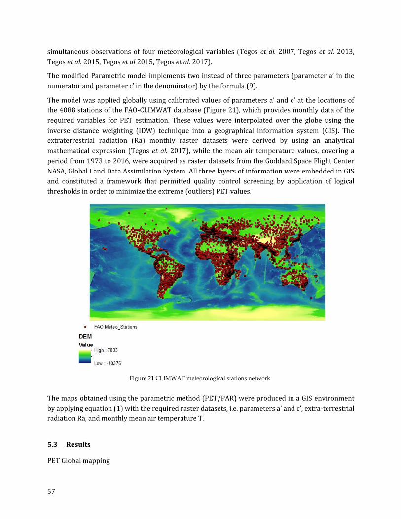
57
simultaneous observations of four meteorological variables (Tegos et al. 2007, Tegos et al. 2013,
Tegos et al. 2015, Tegos et al 2015, Tegos et al. 2017).
The modified Parametric model implements two instead of three parameters (parameter a’ in the
numerator and parameter c’ in the denominator) by the formula (9).
The model was applied globally using calibrated values of parameters a’ and c’ at the locations of
the 4088 stations of the FAO-CLIMWAT database (Figure 21), which provides monthly data of the
required variables for PET estimation. These values were interpolated over the globe using the
inverse distance weighting (IDW) technique into a geographical information system (GIS). The
extraterrestrial radiation (Ra) monthly raster datasets were derived by using an analytical
mathematical expression (Tegos et al. 2017), while the mean air temperature values, covering a
period from 1973 to 2016, were acquired as raster datasets from the Goddard Space Flight Center
NASA, Global Land Data Assimilation System. All three layers of information were embedded in GIS
and constituted a framework that permitted quality control screening by application of logical
thresholds in order to minimize the extreme (outliers) PET values.
Figure 21 CLIMWAT meteorological stations network.
The maps obtained using the parametric method (PET/PAR) were produced in a GIS environment
by applying equation (1) with the required raster datasets, i.e. parameters a’ and c’, extra-terrestrial
radiation Ra, and monthly mean air temperature T.
5.3 Results
PET Global mapping

58
Following the above presented procedures, a monthly PET global dataset was produced covering a
significant time period. Figure 22Figure 23Figure 24 visualize the PET distribution for
representative months across the continents.
Specifically, Figure 22 presents the PET map of Eurasia for August, where PET values range from 0
to 15 mm day–1, increasing from north to south. The latter is well explained from the similar
variation of temperature and extraterrestrial radiation. The highest values were observed at the
Middle East where extremely arid climatic conditions occur.
Figure 22 Eurasia PET map for August (PET: mm/day)
Figure 23 portays the PET pattern in North America for May. A pattern similar to Eurasia is obvious
with highest values at regions near the equator (e.g. Mexico) ,and lowest in Canada and Alaska and
Greenland. PET variability in South America in January with values decreasing from north to south.
Some inconsistencies in the area of Amazon and some peculiarly low values in the area of equator
can be explained from the limitations of the Parametric model to represent the combined effect on
PET estimation of relative humidity and wind speed, which are key drivers of the
evapotranspiration processes across these areas, influencing the net incoming solar radiation and
the evaporation demand, as detailed in Tegos et al. (2017).
Figure 23 North America PET map for May- South America PET map for January (PET: mm/day)
PET variability over Africa in January is shown in Figure 24. High monthly PET values were
acquired in the equatorial zone, mainly in the lower Congo, where the hydro-meteorological

59
observations were limited during the parametric model calibration. The decreasing trend from
south to north in Oceania follows the pattern of radiation and air temperature variation.
Figure 24 Africa/Oceania PET map for January-Oceania PET for December (PET: mm/day)
5.4 Validation
For identifying the efficiency of the PET remote sensing dataset we compared PET/PAR monthly
sample the against a Penman Monteith timeseries, estimated at the Davis station of the well-known
PET data of CIMIS network. The validation was carried out for 3-years periods from 1/2010 to
12/2012 and the coefficient of efficient (CE) was satisfactory equal to 87.6%.
5.5 Further PET improvements
Having reviewed new remote monthly temperature dataset which are recently freely available, we
reassessed the monthly PET with a recently published monthly dataset which provides high global
temperature accuracy (Hooker et al. 2018).
Following the above mentioned framework the monthly PET maps were produced and a first
validation with site meteorological estimate for the Davis station is shown in Figure 25. The
preliminary results are very satisfactory since the coefficient of efficiency is 93.2%. The new
monthly PET dataset based on remote monthly temperature is named RASPOTION and is object for
further validation across the globe.

60
Figure 25 Monthly PM point vs RASPOTION estimate (Davis Station)
5.6 Discussion
In some areas with high values of relative humidity and wind speed, the existing PET parametric
approach fails to reproduce efficiently the PET regime and further improvements of the parametric
approach are recommended locally.
In some areas the FAO-CLIMWAT data were scarce and poor (i.e Brazil and Rebublic of Congo). In
these areas the calibrated parameter a’ and c’ are indicative and further calibration should take
place.
In every case, hydrologists, agronomists and other scientists of potential interest for this dataset
could make efficient use of it, in about 80% of the earth’s territory based on our previous studies
(Tegos et al. 2015, Tegos et al. 2017). The new datasets could provide positive benefits in the
scientific disciplines by taking in to account the global PET datasets are non available, thus is of
interest:
In the applications of physical –based hydrological model which use as PET as an input descriptor
of the sub-catchment, since we are moving forward in global scale hydrological models.
In the crop demand assessment since the integration of the monthly PET and the cropping pattern
quantify the monthly water needs at each type of plant.
5.7 Conclusions
As part of the PET Parametric model, a new global PET monthly dataset based on remote sensing
temperature data was introduced covering the period 1973-2016. This global dataset was extracted

61
using the Parametric formula which uses as input variables the extraterrestrial radiation and the
mean air temperature. The latter have been taken from a freely available dataset provided by NASA.
Further analysis was made with new temperature dataset resulting a new promising PET dataset
namely RASPOTION. Previous analyses with this approach showed satisfying performance, through
validation under several climatic regimes and different validation procedures. In regions where the
available hydro-meteorological information was scarce or insufficient, the modelling results were
weak in terms of PET’s physical interpretation. In these areas the PET/PAR should be used with
caution. Overall, for the majority of the Earth’s globe surface a reliable monthly PET dataset is
compiled and is freely available to scientists across different research disciplines in order to assist
decisions for both short- and long-term hydro-climatic policy actions.
62
6 Investigation of long-term persistence in PET
6.1 A summary on the long-term persistence behaviour
The high complexity and uncertainty of climate dynamics has been long identified through plain
observations as well as extended analyses of hydrometeorological processes such as temperature,
humidity, surface wind, precipitation, atmospheric pressure, river discharges etc. Particularly, all
these processes from global and local scale analyses seem to exhibit the so-called clustering
behaviour (Dimitriadis, 2017). Interestingly, this HK behaviour has been first identified in Nature
by Hurst (1951) while analyzing water levels from the Nile for optimum dam design. However, the
mathematical description and analysis of this behaviour through a power-law autocorrelation
function (vs. lag) is attributed to Kolmogorov (1940) who developed it earlier while studying
turbulence. To give credits to both scientists Koutsoyiannis (2010) named this behaviour as Hurst-
Kolmogorov (HK) behaviour (Dimitriadis, 2017).
6.2 Introduction
Trend estimation in hydro-climatic time series has focused the attention of the scientific
community (Sen, 2013). Many studies have examined the trend of precipitation, streamflow,
groundwater regime, temperature, potential evapotranspiration both in annual and seasonal basis
(Markonis et al. 2016, Stevens et al. 2016, Panda et al. 2012, Arora et al. 2005, Kumar et al. 2010).
Specifically, trend estimation in the potential or actual evapotranspiration pay the attention of the
researchers (Gocic and Trajkovic, 2014, Mo et al. 2015, Tabari et al., 2011). Generally, the trend
results are mixed across different climatic regions, as Tabari et al (2011) found a positive trend for
70% of 20 Iranian meteorological stations during the period 1996-2005, Gocic and Trajkovic
(2014) calculated a significant increasing downward trend in 70% of 12 Serbian meteorological
stations (study period 1980-2010). Finally, Mo et al. 2015, by investigating the areal
evapotranspiration in China for the period 1981-2010 with remote sense data, observed an
increasing trend from the 1980s to the mid-1990s, followed by a decreasing trend. For the
examination of the physical variability, the Mann-Kendall under the independence assumption has
been proposed as a standard statistical measure for the evaluation and the quantification of the
trends (Ahn and Palmer, 2015).
Furthermore, different statistical methodologies have developed and proposed, namely the Mann–
Kendall under the Markovian behavior assumption after trend-free pre-whitening, the Mann–
Kendall with complete autocorrelation structure and the Mann–Kendall under the long-term
persistence assumption (Kumar et al. 2009). The latter test, proposed by Hamed (2008) offers a
consistent framework to consider the Hurst phenomenon, which is observed in many climatological
and hydrological processes, resulting in the increase of physical variability (Koutsoyiannis 2003;
Koutsoyiannis and Montanari 2007). Hurst coefficient was first introduced by engineer Harold
Hurst during the design of the Aswan reservoir (Sutcliffe et al. 2016) and plays a significant role in
63
the hydrological variability (O’Connell et al, 2016). Its presence in large measured
hydrometeorological samples is ubiquitous (Iliopoulou et al. 2016) Comparative analysis of
different trend model shows significant differences in the totally results (Hamed 2008, Kumar et al.
2009) and thus a physical consistent framework is needed.
The following chapters present an R function embedded in an automatic and user-friendly
environment following modern views of water resources modeling tools (Guo et al. 2016, Turner
and Ganelli 2016). The package implements the modified Hamed’s (2008) framework and the
procedure is tested in annual parametric PET time series from 10 sites in Greece, which cover the
period 1950-2000.
6.3 Materials and methods
6.3.1 Mann-Kendall test under the scaling hypothesis
The Mann-Kendall test under the scaling hypothesis consists of three consecutive hypothesis tests,
namely O (Original MK test), H (Hurst Parameter test) and M. The mathematic background and
framework are presented from Hamed (2008). Let H0i denote the null hypothesis of each test and
let H1i denote the alternative hypothesis, where i = O, H, M denotes the step of the Mann-Kendall
test under the scaling hypothesis. We define:
H0O: No trend under the independence assumption
H1O: Significant trend under the independence assumption.
H0H: No significant LTP.
H1H: Significant LTP.
H0M: No trend under LTP assumption.
H1M: Significant trend exists under LTP assumption.
Then the three steps of the test are summarized by the following sequences
{H0O}: No trend.
{H1O}: Possible significant trend. Proceed to step H.
{H1O, H0H}: Significant trend exists.
{H1O, H1H}: Possible LTP effect. Proceed to step M.
{H1O, H1H, H0M}: No trend.
{H1O, H1H, H1M}: Significant trend exists.
Hurst coefficient can be defined by a simple power-law relationship of its standard deviation:
(25)

64
where σ ≡ σ(1) and H is the entropy production in logarithmic time (Koutsoyiannis 2011), and the
parameter ranges between 0 and 1. For values H > 0.5, the process exhibits long-term persistence,
while for H < 0.5 the process is anti-persistent.
For the test implementation, the R function MannKendallLTP from the HKprocess R package
(Tyralis, 2015) was used. The R function computes the p-value in each step of the test. If the p-value
is higher than a predefined significance level α (e.g. α = 0.05), then we cannot reject H0. A p-value
less than or equal to α gives evidence that H1 is true.
6.3.2 Study area and procedures
Ten meteorological stations (National Meteorological Services of Greece) well- distributed over
Greece were used. Table 23 presents the list of the meteorological stations used in our study.
Table 23. Meteorological stations with their latitude (φο) and elevation (z). Stations φ(o) z (m)
Heraklion 35.20 39 Ioannina 39.42 484
Kavala 40.54 63 Kerkyra 39.37 2 Kozani 40.18 626 Larissa 39.39 74 Lemnos 39.54 17 Methoni 36.50 34 Skyros 38.54 5 Tripoli 37.32 663
Based on our previous study (Tegos et al. 2013) the parametric model was calibrated and tested in
monthly time step for the period 1968-1989. For the purposes of this study, monthly air
temperature data for the period 1950-2000 were collected and the parametric model was applied
to the total length. Finally, every monthly time series was aggregated in annual step with the use of
HYDROGNOMON software (Kozanis et al. 2010).
6.3.3 Results
Table 24 presents the results of our analysis. In seven out of the ten stations tested, no trends were
found under the independence assumption. The estimate of the Hurst parameter for annual PET
time series varies in the range 0.43 to 0.76. Out of the three stations that had significant trends
under the independence assumption, only two stations (Ioannina, Lemnos) showed a significant
downward trend.

65
Table 24. Summary results of the application of the Mann-Kendall modified test to the PET data. The Hurst parameter was estimated using the maximum likelihood estimator (Tyralis and Koutsoyiannis 2011). The
trend identification is performed for a predefined level α = 0.05 in each step. Stations Hurst
parameter
estimate
Mann-Kendall 2-
sided p-value
(Step O)
Significance of H,
2-sided p-value
(Step H)
Mann-Kendall LTP
2-sided p-value
(Step M)
Trend identification
Heraklion 0.67 0.31 {H0O}, no trend
Ioannina 0.58 0.05 0.27 {H1O,H0H}, trend
exists
Kavala 0.76 0.63 {H0O}, no trend
Kerkyra 0.71 0.90 {H0O}, no trend
Kozani 0.63 0.31 {H0O}, no trend
Larissa 0.76 0.04 0.00 0.42 {H1O,H1H,HOM} no
trend
Lemnos 0.74 0.00 0.26 {H1O,H0H}, trend
exists
Methoni 0.69 0.06 {H0O}, no trend
Skyros 0.46 0.40 {H0O}, no trend
Tripoli 0.43 0.46 {H0O}, no trend
In Figure 26 PET in Ioannina is presented . In Table 23 we observe a significant trend under the
independence assumption is observed. This assumption is valid. At Kerkyra (see Figure 27) there is
no any significant trend. At Larissa (Figure 28), a significant trend under the independence
assumption is detected; however, this trend is not significant under the long-term dependence
assumption. Finally, we observe a significant trend under a valid independence assumption at
Lemnos is observed (Figure 29).

66
Figure 26. Annual PET at Ioannina
Figure 27. Annual PET at Kerkyra
Figure 28. Annual PET at Larissa

67
Figure 29. Annual PET at Lemnos
6.3.4 Discussion and conclusions
An R function that implements the Mann- Kendall test under the long-term persistence hypothesis
was presented. The test applied and tested in annual time series of PET estimated from a recent
parametric approach. The parametric model estimation allows the consistent estimation of the PET
with minimal data requirements and it's useful for climatic studies when crucial
hydrometerological data are missing (wind velocity, relative humidity, extraterrestrial radiation).
The results of our preliminary case study analysis show that in seven cases, no significant trend was
detected under the independence assumption. In one case, no significant trend was detected under
the long-term persistence assumption, while the trend was significant under the independence
assumption. In the remaining two cases, we found a significant downward trend under both the
independence and the long-term persistence assumptions. In total, an R function is ready and user-
friendly for extensive use in other field of water resources and technological- related studies.
6.4 Temperature variability over Greece : Links between space and time
The long-term alteration of the meteorological paid the attention of the scientific community the
last decades by linking it with the well-known “climate-change” interest. It is therefore necessary to
examine long term instrumental observations or reliable estimate to quantify the fluxes trends. In
this respect, meteorological data from 35 stations of HNMS were collected and used (monthly
timeseries 1950-2000), with a rather uniform spatial distribution as it can be seen Figure 30.
For studying the climatic behaviors the stations was classified in three categories: continental,
coastal and inland stations.

68
Figure 30. Study Area- meteorological stations locations
Attention was paid to the temperature monthly dataset and as visualizes the Figure 31 the inter-
annual variation (i.e. the mean standard deviation of the monthly temperatures of each year) shows
that the variability of temperature parameters is higher to continental stations than to coastal or
island regions.

69
Figure 31. Inter-annual temperature variability
Overall, temperature in Greece has been relatively stable for the last 50 years as shown in the
Figure 32.
Figure 32. Study Area- locations of meteorological stations
Monthly potential evapotranspiration for each station was estimated by the parametric model
(Tegos et al. 2013, Tegos et al. 2015): dependent only to temperature Tα and incoming solar
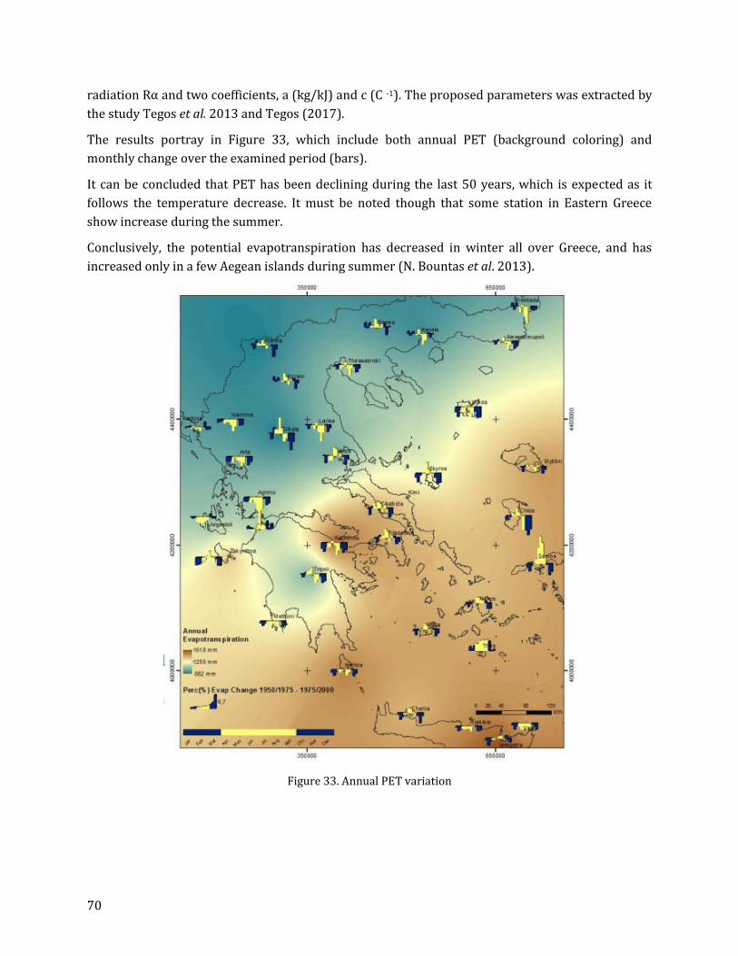
70
radiation Rα and two coefficients, a (kg/kJ) and c (C -1). The proposed parameters was extracted by
the study Tegos et al. 2013 and Tegos (2017).
The results portray in Figure 33, which include both annual PET (background coloring) and
monthly change over the examined period (bars).
It can be concluded that PET has been declining during the last 50 years, which is expected as it
follows the temperature decrease. It must be noted though that some station in Eastern Greece
show increase during the summer.
Conclusively, the potential evapotranspiration has decreased in winter all over Greece, and has
increased only in a few Aegean islands during summer (N. Bountas et al. 2013).
Figure 33. Annual PET variation

71
7 Applications in agricultural design
7.1 Spatial interpolation methods in PET estimate
7.1.1 Introduction
Potential evapotranspiration (PET) is a crucial parameter of several applications in hydrological
modelling, irrigation and environmental studies. Especially, precision irrigation requires daily or
even hourly PET estimates in order to increase the efficiency of water use through optimization
procedures that include the use of sensors along with extensive soil, water and crop data. A
significant concept for precision irrigation design is the spatial variability of the PET since the well-
established FAO Penman-Monteith model (Allen et al. 1998), but also alternative frameworks
(Tegos et al. 2015) provide point estimates.
Precision irrigation constitutes a breakthrough for agricultural water management since it provides
means to optimal water use. In recent years several applications of precision irrigation are
implemented based on spatial data from different origins, i.e. meteorological stations networks,
remote sensing data and in situ measurements. One of the factors affecting optimal irrigation
system design and management is the daily potential evapotranspiration (PET). A commonly used
approach is to estimate the daily PET for the representative day of each month during the irrigation
period. The implementation of the recently introduced non-parametric bilinear surface smoothing
(BSS) methodology for spatial interpolation of daily PET is presented. The study area was the plain
of Arta which is located at the Region of Epirus at the North West Greece. Daily PET was estimated
according to the FAO Penman-Monteith methodology with data collected from a network of six
agrometeorological stations, installed in early 2015 in selected locations throughout the study area.
For exploration purposes, PET maps for the Julian dates: 105, 135, 162, 199, 229 and 259 were
produced, thus covering the entire irrigation period of 2015. Also, comparison and cross validation
against the calculated FAO Penman-Monteith PET for each station, were performed between BSS
and a commonly used interpolation method, i.e. inverse distance weighted (IDW). During the leave-
one-out cross validation procedure, BSS yielded very good results, outperforming IDW. Given the
simplicity of the BSS, its overall performance is satisfactory, providing maps that represent the
spatial and temporal variation of daily PET.
7.1.2 Study area and meteorological stations network
The study area was located at the plain of Arta (453.29 km2, the biggest of the region), at the Region
of Epirus at the north west coast of Greece (Figure 34). It is part of the Arachthos and Louros
hydrological basins and borders with Amvrakikos Wetlands National Park. The local climate is of
Mediterranean type, characterized by dry and hot summers and rainy and moderately cool winters.

72
Figure 34. The Arta plain along with the study area and the agrometeorological stations network
Irrigation in the area is performed by means of surface irrigation, sprinkler irrigation and drip
systems in proportions of about 40%, 40% and 20% respectively (Tsirogiannis and Triantos, 2009),
with a continuous diminution of surface irrigation. The vast majority of farmers irrigate based on
experience and inherited practical advices. As water is plentiful and cheap, most farmers over
irrigate using water by the old open canal scheme that covers part of the plain and from numerous
boreholes.
An agrometeorological stations network of six fully equipped weather stations was installed in
early 2015 for the implementation of IRMA_SYS project (Malamos et al. 2016 -
http://arta.irrigation-management.eu/) in order to monitor evapotranspiration related
parameters. The data from the six meteorological stations are available at http://openmeteo.org/
under Database Contents License v.1.0 for individual measurements and Open Database License
v.1.0 for the data series as they are published at Open Data Commons
(http://opendatacommons.org/).
The analysis extend (mask) boundaries were defined by the coordinates of the outermost stations
according to each one of the four cardinal directions. This was mandatory in order to ensure that
the PET estimates adjacent to the boundaries of the study area are obtained from interpolation
rather than extrapolation. The maps were produced using a 500 × 500 m grid for practical and
computational reasons, covering an area of approximately 294.8 km2 inside the plain of Arta.

73
7.1.3 Spatial interpolation methods
The mathematical framework of Bilinear Surface Smoothing (Malamos and Koutsoyiannis 2016a),
suggests that fit is meant in terms of minimizing the total square error among the set of original
points zi(xi, yi) for i = 1,…, n and the fitted bilinear surface, that in matrix form, can be written as:
(26)
where z = [z1,…, zn]T is the vector of known applicates of the given data points with size n (the
superscript T denotes the transpose of a matrix or vector) and ,…, is the vector of
estimates with size n.
The details of the method including the algorithms and derivations of the equations are available at
(Malamos and Koutsoyiannis 2016a).
The parameters required to implement the methodology, are the segments of the bilinear surface,
i.e. mx, my and the smoothing parameter λ. These parameters can be estimated by transforming the
smoothing parameter λ in terms of tension: τλ whose values are restricted in the interval [0, 1), for
both directions i.e. τλx and τλy (Malamos and Koutsoyiannis 2016a). This transformation provides a
convenient search in terms of computational time and is based on the generalized cross-validation
(GCV - Craven and Wahba 1978) methodology. Thus, for a given combination of segments mx, my,
the minimization of GCV results in the optimal values of τλx, τλy. This can be repeated for several trial
combinations of mx, my values, until the global minimum of GCV is reached.
On the other hand, the Inverse Distance Weighting (IDW) method was implemented as a quick
interpolator capable to address the characteristics of the study area regarding the limited number
of meteorological stations. IDW is a straightforward and non-computationally intensive method
(Burrough and McDonnell 1998). The IDW implementation for producing the PET maps of the
study area was performed by means of ESRI’s ArcGIS environment.
7.1.4 Results and discussion
In order to evaluate the performance of the BSS methodology for spatial interpolation of daily PET,
we interpolated the Penman-Monteith PET values acquired at the stations locations (Table 25)
using both BSS and IDW for the characteristic day of each month for the 2015 irrigation period as
presented in Figure 35 Figure 36.
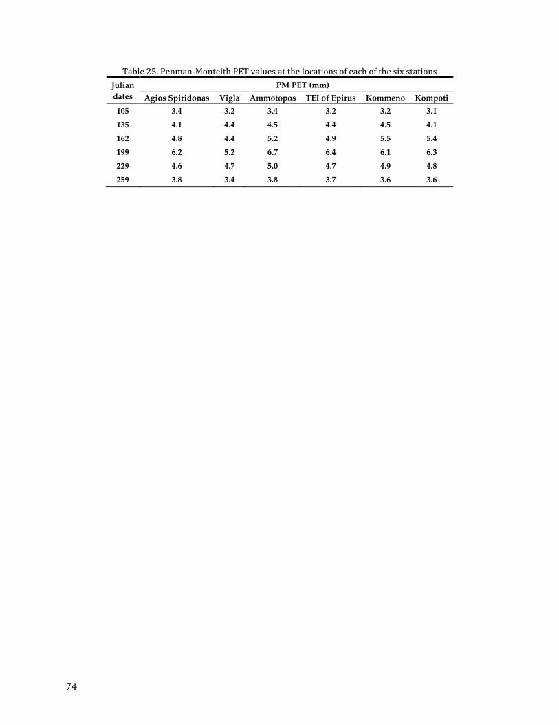
74
Table 25. Penman-Monteith PET values at the locations of each of the six stations
Julian
dates
PM PET (mm)
Agios Spiridonas Vigla Αmmotopos TEI of Epirus Kommeno Kompoti
105 3.4 3.2 3.4 3.2 3.2 3.1
135 4.1 4.4 4.5 4.4 4.5 4.1
162 4.8 4.4 5.2 4.9 5.5 5.4
199 6.2 5.2 6.7 6.4 6.1 6.3
229 4.6 4.7 5.0 4.7 4.9 4.8
259 3.8 3.4 3.8 3.7 3.6 3.6

75
Figure 35. BSS PET maps for Julian dates 105, 135, 162, 199, 229, 259 of year 2015
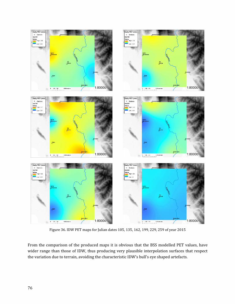
76
Figure 36. IDW PET maps for Julian dates 105, 135, 162, 199, 229, 259 of year 2015
From the comparison of the produced maps it is obvious that the BSS modelled PET values, have
wider range than those of IDW, thus producing very plausible interpolation surfaces that respect
the variation due to terrain, avoiding the characteristic IDW’s bull's eye shaped artefacts.

77
Considering BSS’s implementation, the global minimum of GCV for each day was reached by
implementing it for different numbers of segments mx and my (1 ≤ mx ≤ 15 and 1 ≤ my ≤ 15, while
m + 1 ≥ 6) and minimizing GCV for each one, by altering the adjustable parameters.
The results of the above procedure are presented in Table 26, along with the corresponding mean
square error values. It is obvious that the BSS implementation resulted in very small mean square
error values, respecting the estimated PM PET values at the stations locations. It can be assumed
that there is no need to present the corresponding mean square error values for the IDW at the
given data points i.e. the stations locations, since it is an exact method of interpolation so its results
respect the data points exactly.
Table 26. BSS optimal parameter values and performance indices Julian dates
mx my τλx τλy Mean square
error Global minimum
GCV
105 2 3 0.902 0.154 1.75 10–5 2.93 10–3
135 4 5 0.003 0.765 1.42 10–5 3.76 10–3
162 5 4 0.99 0.001 1.13 10–5 4.95 10–3
199 6 12 0.76 0.019 7.42 10–5 3.15 10–2
229 14 6 0.201 0.001 3.77 10–6 6.35 10–4
259 2 6 0.784 0.067 2.47 10–5 5.11 10–3
Also, the above criteria of performance may not be representative with respect to the validity of the
interpolation results in other locations, except for those incorporated in the interpolation
procedure. So, an alternative technique was implemented for the evaluation of the bilinear surface
smoothing method efficiency, in terms of performing a leave-one-out cross validation procedure of
the two methods. The procedure was implemented in MS-Excel and included a loop in which the
PET values at the location of each station were estimated using the remaining five as the input
dataset to each one of the two interpolation methods. In this way, we acquired a total of six, one for
every day, PET estimates at the stations locations which were compared against the already
acquired daily PM PET values. We should note that BSS was implemented using the previously
obtained parameter values as presented in Table 26.
The performance of each method was evaluated by using statistical criteria such as: mean bias
error (MBE), mean absolute error (MAE), root mean square error (RMSE), mean square error
(MSE) and modelling efficiency (EF) which is calculated on the basis of the relationship between the
observed and predicted mean deviations (Malamos and Koutsoyiannis 2016b). As Table 27 states,
BSS clearly outperformed IDW in all circumstances, apart from the EF and RMSE criteria at the
Kompoti station. In this case, both methods failed to provide satisfactory estimates of PET values.
An explanation to this behaviour is the fact that the Kompoti station is placed on the east side of the
study area close to the mountains so when it is missing, the available information is inadequate to
describe the orography effects, thus resulting in insufficient estimates.

78
Table 27. Performance of BSS and IDW against PM PET values in the leave-one-out cross validation procedure
Agios Spiridonas Vigla Ammotopos
TEI of Epirus
Kommeno Kompoti
BSS IDW BSS IDW BSS IDW BSS IDW BSS IDW BSS IDW
MBE (mm) 0.0 0.8 0.0 0.4 0.0 0.4 0.0 0.1 -0.5 1.6 -1.7 1.7
MAE (mm) 0.1 0.8 0.1 0.4 0.0 0.4 0.1 0.1 0.5 1.6 1.7 1.7
RMSE (mm) 0.1 0.8 0.2 0.5 0.1 0.4 0.1 0.1 0.8 1.6 1.9 1.7
EF 0.99 0.18 0.95 0.47 1.00 0.85 0.99 0.98 0.44 -
1.55 -2.02
-1.44
7.1.5 Conclusions
Two different approaches for spatial interpolation of daily potential evapotranspiration were
implemented using data from six meteorological stations located in the plain of Arta, at the Region
of Epirus. Both approaches were implemented for the characteristic day of each month for the 2015
irrigation period, i.e. Julian dates: 105, 135, 162, 199, 229 and 259. The objective was to evaluate
the performance of bilinear surface smoothing (BSS) method against the inverse distance weighting
(IDW) method. The comparison against the estimated values of the FAO Penman-Monteith (PM)
PET for each station showed that BSS yielded very good results with very small mean square error
values, respecting the given PM PET values.
Also, a leave-one-out cross-validation procedure per station was used for validating the
performance of both spatial interpolators. Thus we acquired a total of six, one for every day, PET
estimates at the stations locations which were compared against the already acquired daily PM PET
values. During this cross validation procedure BSS clearly outperformed IDW in almost every case,
respecting the variation of the terrain and also avoiding the characteristic IDW’s bull's eye shaped
artefacts. Given the simplicity of the BSS methodology, its overall performance is satisfactory,
providing maps that represent the spatial and temporal variation of daily PET, thus granting the
necessary tools for implementing precision irrigation on daily or finer time scale.
7.2 Regional daily/monthly parametric model in Arta valey
7.2.1 Introduction
The parametric model was applied in the Arta a strong irrigated value in western East of Greece
(Figure 37).

79
Figure 37. Study Area
Meteorological data was collected from 3 meteorological stations and the following computational
procedures was made:
Calibration of the using historical data from 3 stations and regionalization of the parameters
throughout Arta plain. Fit of the parametric formula at daily and monthly in the samples of
the three stations and extraction of the parameters a,b,c. High CE was observed for the
parametric model using PM as base sample.
Regionalization of daily and monthly temperatures from 6 stations located in Arta plain
using I.D.W method as providing by a newer meteorological network.
Production of 10 raster maps (5 for mean monthly temperature and 5 for mean daily day of
the 15th day of each month)
Appropriate coding of extraterrestrial radiation and production of the corresponding raster
files
7.2.2 Daily PET Spatial variability
Figure 38 illustrates the spatial variation of PET at each month. The main outcomes are as follows:
PET high values are observed in North for every month and low values in the South adjacent
to the shore.
Mean daily ranges from 2 mm (April) to 4.9 mm (July).
Significant PET spatial variation in daily scale and for all months.
Non standard spatial direction for every month in the study period.
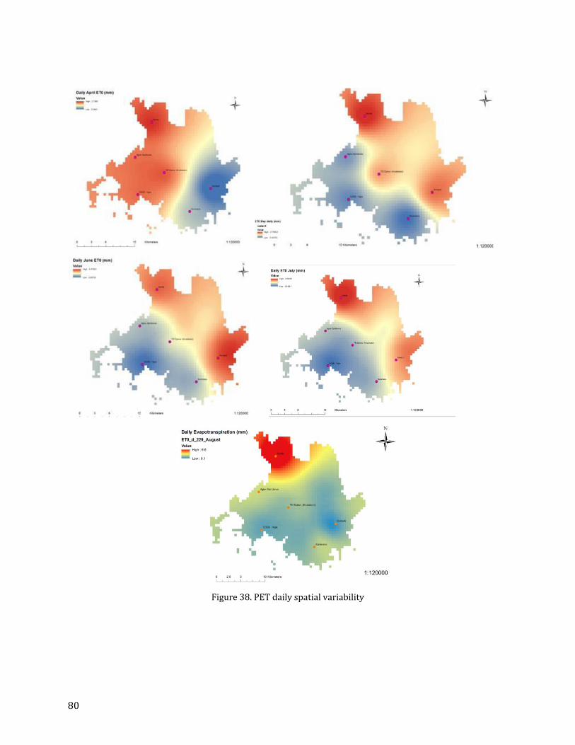
80
Figure 38. PET daily spatial variability

81
7.2.3 Monthly PET Spatial variability
Figure 39 visualizes PET monthly variability for each month. In respect the results it can be
concluded the following:
Gradient of the monthly PET from North to South direction (limited in April)
Mean monthly PET ranges between 80.6 mm (April) to 174 mm (July)
Insignificant spatial variation for spring months (April, May) and significant in summer
months (June, July, August)
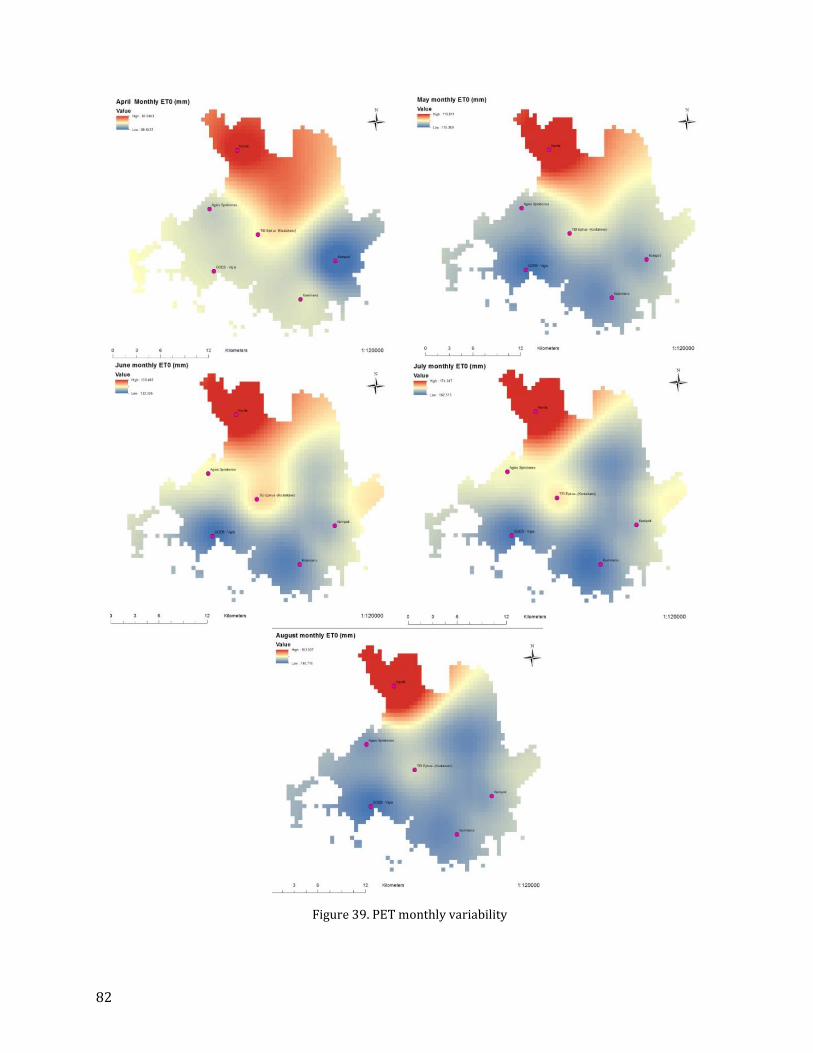
82
Figure 39. PET monthly variability

83
8 Conclusions and Discussion
The major innovations of the thesis is the development of a new parametric radiation-based PET
model which can be considered as simplification of the Penman-Monteith formula, in an attempt to
combine parsimony, in terms of model structure and data requirements, and physical consistency.
The parametric model is a parsimonious radiation-based and physically consistent approach
derived from a simplification of the Penman-Monteith equation. It requires in its first exhibition
three parameters to be calibrated prior to its application and two parameters in its second global
format. Specifically, two model versions were presented in this respect, the first one was applied in
the well-known CIMIS network and the second a slightly modifications of the first expression in the
Global Dataset of CLIMWAT.
The model ensures excellent predictive capacity (in terms of reproducing monthly PET estimations
through the Penman-Monteith) in the majority of the examined in both applications. In the first
application (CIMIS), the model outperforms all the radiation-based and empirical formulas and in
the global application provided better performance in comparison with the Hargreaves model. It’s
worth mentioning that a main hint point of this thesis is that the local calibration of the simplified
models is reqired, in assessing consistent PET since the comparisons across different climates
reveal the great advantage of parametric approaches against radiation-based ones, since calibration
allows the coefficients that are involved in the mathematical formulas to be fitted to local climatic
conditions. The parameters of the new model have some physical background, since they
substitute, to some extent, the three missing meteorological variables namely the humidity, the
wind velocity and the radiation. Taking into account the limited availability of data capable to
acquire the set of parameters of the Parametric method into timescales finer than monthly e.g. daily
or even hourly, an interesting study could be the investigation of downscaling them against time.
This investigation might be performed by applying a regression analysis that involves establishing a
mathematical relationship between the large scale acquired parameters against those of finer scale.
Another point of interest of this thesis was the investigation of the optimal spatial technique in
converting the point scale estimate into regional, by implementing interpolation techniques such
as: Inverse Distance Weighting (IDW), Natural Neighbours (NaN), Ordinary Kriging (OK) and
Bilinear Surface Smoothing (BSS), along an extensive study area such as California. The validation
procedure was implemented by comparing the reference potential evapotranspiration estimates
acquired from the implementation of the parametric method, using the parameter estimates of the
four interpolation methods, against those of the eleven additional CIMIS stations. This combined
evaluation of the four different interpolation approaches, indicated that the simple and effortless
IDW method performs better than the other three methodologies. Regarding the application of the
new methodology, BSS’s efficiency to perform interpolation between data points that are
interrelated in a complicated manner was confirmed, acquiring high CE values analogous to those
of the other three methods. In this light, global parameters map was provided using IDW for direct
application of the parametric expression across the globe.

84
Numerous applications were presented including the development of a R software script for
estimating the annual trend under Hurst-Kolmogorov behavior and a global remote sensing PET
monthly dataset.
Incidental contributions, moderate innovations and future research required are summarized
below:
Future research attempt requires a detailed investigation of the factors affecting the model poor
performance in specific areas over the globe, in order to recognize whether these can be handled
through a slightly different model structure or they do require the use of additional explanatory
variables or parameters. Apparently, this will require the use of full meteorological time series
instead of climatic data, which is a very challenging task at global scale. Another challenging task is
a survey of the calibration results against different climatic zones that will further highlight the
model advantages, as well as potential shortcomings.
Since the need of the large-scale hydrological modeling is under high development at least last
decade, the Global PET maps at multiple time scale extracted by in-situ measurements or by
combining remote sensing measurements can be support the hydrological community by providing
reliable PET estimates which are required input-data in numerous well known model such as
SWAT. To achieve that, future research shall focus in the production of reliable PET estimate
integrating site temperature and remote sensing samples. A first which was presented in this
Thesis is very promising since the new PET monthly dataset (RASPOTION) provided very
satisfactory results.
Reliable global PET estimate could be useful and in another hydrological science field referring to
the low-flow assessment in ungauged catchments. Typically, the most recent scientific attempts in
this regard use the PET as explanatory variable of regression models and therefore PET accuracy is
noteworthy for estimating the flow duration curves in ungauged catchments.
Another interesting for further research survey is the use of the parametric framework within the
field of agronomical studies and especially in the forecasting of the crop water requirements for
scheduling the irrigation program in timely manner. The key idea of the Parametric model owing to
minimal input data requirements can be decrease the overall uncertainty of the PET projection at
short-term forecast (up to 3-days) and therefore the short term weather prediction can be
incorporated to an efficiency Decision Support System for the crop assessment in local and large
scale precision agriculture.
Conclusively, the Parametric Model is a robust model with numerous potential applications in
different disciplines related to hydrology and geosciences as well, since PET is a critical input
variable of hydrological modeling, in assessing the crop water demands of several agronomist
studies, in physical based estimation of the low flow in ungauged catchments, in assessing the long-
term trends of hydrometerological variables.

85
References
Ahn, K. H., & Palmer, R. N. (2015). Trend and Variability in Observed Hydrological Extremes in the
United States. Journal of Hydrologic Engineering, 21(2), 04015061.
Alexandris, S., Kerkides, P., 2003. New empirical formula for hourly estimations of reference
evapotranspiration. Agric. Water Manag. 60, 157–180.
Allen, R.G., Jensen, M.E., Wright, J.L., Burman, R.D., 1989. Operational Estimates of Reference
Evapotranspiration. Agron. J. 81, 650.
Allen, R.G., L.S. Pereira, D. Raes, & M. Smith, Crop evapotranspiration: Guidelines for computing crop
water requirements, FAO Irrigation and Drainage Paper 56, Rome, 1998.
Allen, R.G.; Pruitt, W.O. Rational use of the FAO Blaney-Criddle formula. J. Irrig. Drain. Eng. 1986,
112, 139–155.
Amatya, D.M.; Skaggs, R.W.; Gregory, J.D. Comparison of methods for estimating REF-ET. J. Irrig.
Drain. Eng. 1995, 121, 427–435.
Arora, Manohar, N. K. Goel, and Pratap Singh. "Evaluation of temperature trends over
India."Hydrological sciences journal 50.1 (2005).
Azhar, A.H., Perera, B.J.C., 2011. Evaluation of Reference Evapotranspiration Estimation Methods
under Southeast Australian Conditions. J. Irrig. Drain. Eng. 137, 268–279.
Blaney, H.F., Criddle, W.D., 1962. Determining consumptive use and irrigation water requirements
(No. 1275). US Department of Agriculture.
Bhattarai, N., Dougherty, M., Marzen, L.J. and Kalin, L., 2012. Validation of evaporation estimates
from a modified surface energy balance algorithm for land (SEBAL) model in the south-eastern
United States. Remote sensing letters, 3(6), pp.511-519.
Birhanu, D., Kim, H., Jang, C., & Park, S. (2018). Does the Complexity of Evapotranspiration and
Hydrological Models Enhance Robustness?. Sustainability, 10(8), 2837.
Burrough, P.A. and McDonnell, R.A., 1998. Principles of Geographical Information Systems. New
York: Oxford University Press.
Choudhury, B.J., 1997. Global pattern of potential evaporation calculated from the Penman-
Monteith equation using satellite and assimilated data. Remote Sensing of Environment, 61(1),
pp.64-81.
Craven, P. and Wahba, G., 1978. Smoothing noisy data with spline functions - Estimating the correct
degree of smoothing by the method of generalized cross-validation. Numerische Mathematik, 31
(4), 377–403.

86
Dalezios, N.R.; Loukas, A.; Bampzelis, D. Spatial variability of reference evapotranspiration in
Greece. Phys. Chem. Earth Parts A/B/C 2002, 27, 1031–1038.
Dimitriadis, P., Hurst-Kolmogorov dynamics in hydroclimatic processes and in the microscale of
turbulence, Ph.D thesis, Department of Water Resources and Environmental Engineering –
National Technical University of Athens, 2017.
Dingman, S.L. Physical Hydrology; MacMillan Publishing Company: New York, NY, USA, 1994.
Doorenbos, J.; Pruitt, W.O. Guidelines for predicting crop water requirements: Rome, Italy, food and
agricultural organization of the United Nations. FAO Irrigation and Drainage Paper 24, 1977)
Droogers, P., & Allen, R. G. (2002). Estimating reference evapotranspiration under inaccurate data
conditions. Irrigation and drainage systems, 16(1), 33-45.
Efstratiadis, A.; Koutsoyiannis, D. One decade of multiobjective calibration approaches in
hydrological modelling: A review. Hydrol. Sci. J. 2010, 55, 58–78.
Efstratiadis, A.; Koutsoyiannis, D. An evolutionary annealing-simplex algorithm for global
optimisation of water resource systems. Hydroinformatics 2002: Proceedings of the Fifth
International Conference on Hydroinformatics, International Water Association: London, UK,
2002; pp.1423–1428.
FAO. CLIMWAT for CROPWAT, A climatic database for irrigation planning and management, FAO
Irrigation & Drainage Paper No. 49, Rome, 1993. Available online:
http://www.fao.org/nr/water/infores_databases_climwat. html
Farquhar, G.D., Roderick M.L., 2007. Worldwide changes in evaporative demand, Proceedings of the
Pontifical Academy of Sciences, 2005.
Fooladmand, H.R.; Haghighat, M. Spatial and temporal calibration of Hargreaves equation for
calculating monthly ET0 based on Penman‐Monteith method. Irrig. Drain. 2007, 56, 439–449.
Foyster, A.M. Application of the grid square technique to mapping of evapotranspiration. J. Hydrol.
1973, 19, 205–226.
Gavilán, P.; Lorite, I.J.; Tornero, S.; Berengena, J. Regional calibration of Hargreaves equation for
estimating reference ET in a semiarid environment. Agric. Water Manag. 2006, 81, 257–281.
Ghilain, N. and Gellens-Meulenberghs, F., 2014. Assessing the impact of land cover map resolution
and geolocation accuracy on evapotranspiration simulations by a land surface model. Remote
sensing letters, 5(5), pp.491-499.
Gocic, Milan, and Slavisa Trajkovic. "Analysis of trends in reference evapotranspiration data in a
humid climate."Hydrological Sciences Journal 59.1 (2014): 165-180.

87
Guo, D., Westra, S., & Maier, H. R. (2016). An R package for modelling actual, potential and reference
evapotranspiration. Environmental Modelling & Software, 78, 216-224
Guo, D.; Westra, S.; Maier, H.R. Sensitivity of potential evapotranspiration to changes in climate
variables for different climatic zones. Hydrol. Earth Syst. Sci. 2016, 1–43.
Hamed KH (2008) Trend detection in hydrologic data: The Mann-Kendall trend test under the
scaling hypothesis. Journal of Hydrology 349(3-4):350-363.
Hargreaves G.H, and Z.A. Samani Z.A, Estimating potential evapotranspiration, Technical note, J.
Irrig. Drain.e Eng., 108(3), 225-300, 1982.
Hansen S. Estimation of potential and actual evapotranspiration.Nordic Hydrol 1984, 15:205–212
Hargreaves G. H.; Samani, Z. A. Reference crop evaporation from temperature. Appl. Eng. Agric.
1985, 1, 96–99.
Hart, Q.J., Brugnach, M., Temesgen, B., Rueda, C., Ustin, S.L., Frame, K., 2009. Daily reference
evapotranspiration for California using satellite imagery and weather station measurement
interpolation. Civ. Eng. Environ. Syst. 26, 19–33.
Haslinger, K.; Bartsch, A. Creating long-term gridded fields of reference evapotranspiration in
Alpine terrain based on a recalibrated Hargreaves method. Hydrol. Earth Sys. Sci. 2016, 20,
1211–1223.
Hooker, J., Duveiller, G., & Cescatti, A. (2018). A global dataset of air temperature derived from
satellite remote sensing and weather stations. Scientific data, 5(1), 1-11.
Hu, Q.F.; Yang, D.W.; Wang, Y.T.; Yang, H.B. Global calibration of Hargreaves equation and its
applicability in China. Adv. Water Sci. 2011, 22, 160–167.
Iliopoulou, T., Papalexiou, S. M., Markonis, Y., & Koutsoyiannis, D. (2016). Revisiting long-range
dependence in annual precipitation. Journal of Hydrology.
Irmak, S., Allen, R.G., Whitty, E.B., 2003. Daily Grass and Alfalfa-Reference Evapotranspiration
Estimates and Alfalfa-to-Grass Evapotranspiration Ratios in Florida. J. Irrig. Drain. Eng. 129,
360–370.
Jensen, M.E., Haise, H.R., 1963. Estimating evapotranspiration from solar radiation. Proc. Am. Soc.
Civ. Eng. J. Irrig. Drain. Div. 89, 15–41.
Jensen M., and H. Haise, Estimating evapotranspiration from solar radiation, J. Irrig. Drain. Div.,
89(1R4), 15–41, 1989.
Kitanidis, P.K. Introduction to Geostatistics: Applications in Hydrogeology; Cambridge University
Press: New York, NY, USA, 1997.

88
Klok, E.J., Klein Tank, A.M.G., 2009. Updated and extended European dataset of daily climate
observations. Kozanis, S., Christofides, A., Mamassis, N., Efstratiadis, A., Koutsoyiannis D., 2010.
Hydrognomon – open source software for the analysis of hydrological data, EGU General
Assembly 2010, Geophysical Research Abstracts, Vol. 12, Vienna, 12419.
Kozanis, S., Christofides, A., Mamassis, N., Efstratiadis, A. and Koutsoyiannis, D., 2010, May.
Hydrognomon–open source software for the analysis of hydrological data. In EGU General
Assembly Conference Abstracts (Vol. 12, p. 12419).
Koutsoyiannis, D.; Mamassis, N.; Tegos, A. Logical and illogical exegeses of hydrometeorological
phenomena in ancient Greece. Water Sci. Technol.: Water Supply 2007, 7, 13–22.
Koutsoyiannis, D., 2003. Climate change, the Hurst phenomenon, and hydrological statistics.
Hydrological Sciences-Journal-des Sciences Hydrologiques 48 (1).
Koutsoyiannis, D., 2009. Seeking parsimony in hydrology and water resources technology
(solicited), European Geosciences Union General Assembly 2009, Geophysical Research
Abstracts, Vol. 11, Vienna, 11469. (http://www.itia.ntua.gr/en/docinfo/906/)
Koutsoyiannis, D., 2014. Reconciling hydrology with engineering. Hydrol. Res. 45 (1), 2-24.
Li, J., Heap, A.D., 2008. A Review of Spatial Interpolation Methods for Environmental Scientists,
Geoscience Australia. Geoscience Australia, GPO Box 378, Canberra, ACT 2601, Australia.
Koutsoyiannis D. 2011. Hurst–Kolmogorov dynamics as a result of extremal entropy production.
Physica A: Statistical Mechanics and its Applications, 390(8): 1424-1432
Koutsoyiannis, D., and Th. Xanthopoulos, Engineering Hydrology, National Technical University of
Athens, 1999.
Koutsoyiannis, D., Hydrology and Change. Hydrol. Sci. J. 2013, 58, 1177–1197.
Koutsoyiannis, D., Montanari, A., 2007. Statistical analysis of hydroclimatic time series: uncertainty
and insights. Water Resources Research 43, W05429.
Kumar, S., Merwade, V., Kam, J., & Thurner, K. (2009). Streamflow trends in Indiana: effects of long
term persistence, precipitation and subsurface drains. Journal of Hydrology, 374(1), 171-183.
Li, Z.; Chen, Y.; Shen, Y.; Liu, Y.; Zhang, S. Analysis of changing pan evaporation in the arid region of
Northwest China. Water Resour. Res. 2013, 49, 2205–2212.
Lofgren, B.M.; Hunter, T.S.; Wilbarger, J. Effects of using air temperature as a proxy for
evapotranspiration in climate change scenarios of Great Lakes basin hydrology. J. Gt. Lakes Res.
2011, 37, 744–752.

89
Longley, P.A., Goodchild, M.F., Maguire, D.J., Rhind, D.W., 2005. Geographic information system and
Science, second ed, England: John Wiley & Sons, Ltd, West Sussex PO19 8SQ, England, pp. 333–
335.
Lu, J., Sun, G., McNulty, S.G., Amatya, D.M., 2005. A comparison of six potential comparison
evapotranspiration methods for regional use in the Southeastern United States. J. Am. Water
Resour. Assoc. 41, 621–633.
Makkink, G.F. (1957). Testing the Penman formula by means of lysimeters. J. Inst. Water Engng. 11
(3): 277-288
Malamos, N. and Koutsoyiannis, D., 2016a. Bilinear surface smoothing for spatial interpolation with
optional incorporation of an explanatory variable. Part 1: Theory. Hydrological Sciences Journal,
61 (3), 519–526.
Malamos, N. and Koutsoyiannis, D., 2016b. Bilinear surface smoothing for spatial interpolation with
optional incorporation of an explanatory variable. Part 2: Application to synthesized and rainfall
data. Hydrological Sciences Journal, 61 (3), 527–540.
Malamos, N., Tsirogiannis, I.L., and Christofides, A., 2016. Modelling irrigation management
services: the IRMA_SYS case. International Journal of Sustainable Agricultural Management and
Informatics, 2 (1), 1–18.
Malamos, N.; Tegos, A.; Tsirogiannis, I.L.; Christofides, A.; Koutsoyiannis, D. Implementation of a
regional parametric model for potential evapotranspiration assessment. In Proceedings of
IrriMed 2015—Modern Technologies, Strategies and Tools for Sustainable Irrigation
Management and Governance in Mediterranean Agriculture, Bari, Italy, 23–25 September 2015.
Malamos, N.; Tsirogiannis, I.L.; Tegos, A.; Efstratiadis, A.; Koutsoyiannis, D. Spatial interpolation of
potential evapotranspiration for precision irrigation purposes. In Proceedings of 10th World
Congress on Water Resources and Environment, Athens, Greece, 5–9 July 2017.
Mamassis, N., Panagoulia, D., Novcovic, A., 2014. Sensitivity analysis of Penman evaporation
method, Global NEST Journal, Vol.16, No 4, pp. 628-639.
Mancosu, N., Snyder, R.L., Spano, D., 2014. Procedures to Develop a Standardized Reference
Evapotranspiration Zone Map. J. Irrig. Drain. Eng. 140, A4014004.
Mardikis, M.G.; Kalivas, D.P.; Kollias, V.J. Comparison of interpolation methods for the prediction of
reference evapotranspiration—An application in Greece. Water Resour. Manag. 2005, 19, 251–
278.
Markonis, Y., Batelis, S. C., Dimakos, Y., Moschou, E., & Koutsoyiannis, D. (2016). Temporal and
spatial variability of rainfall over Greece. Theoretical and Applied Climatology, 1-16.

90
McGuiness J.L., and E.F. Bordne, A comparison of lysimeter-derived potential evapotranspiration
with computed values, Technical Bulletin 1452, Agricultural Research Service, US Department of
Agriculture, Washington, DC, 1972.
McMahon, T.A., M.C. Peel, L. Lowe, R. Srikanthan, and T.R. McVicar, Estimating actual, potential,
reference crop and pan evaporation using standard meteorological data: a pragmatic synthesis,
Hydrol. Earth Sys. Sci., 17, 1331-1363, 2013.
McMahon, T.A.; Finlayson, B.L.; Peel, M.C. Historical developments of models for estimating
evaporation using standard meteorological data. Wiley Interdiscip. Rev. Water 2016, 3, 788–
818.
McVicar, T.R.; Roderick, M.L.; Donohue, R.J.; Li, L.T.; Van Niel, T.G.; Thomas, A.; Grieser, J.; Jhajharia,
D.; Himri, Y.; Mahowald, N.M.; Mescherskaya, A.V.; Kruger, A.C.; Rehman, S.; Dinpashoh, Y. Global
review and synthesis of trends in observed terrestrial near-surface wind speeds: Implications
for evaporation. J. Hydrol. 2012, 416–417, 182–205.
Merz R.; Blöschl, G. Regionalisation of catchment model parameters. J. Hydrol. 2004, 287, 95–123.
X., Liu, S., Lin, Z., Wang, S., & Hu, S. (2015). Trends in land surface evapotranspiration across China
with remotely sensed NDVI and climatological data for 1981–2010.Hydrological Sciences
Journal, 60(12), 2163-2177.
Mohawesh, O.E. Spatio-temporal calibration of Blaney–Criddle equation in arid and semiarid
environment. Water Resour. Manag. 2010, 24, 2187–2201.
Monteith, J.L., Evaporation and the environment: The state and movement of water in living
organism, XIXth Symposium, Cambridge University Press, Swansea, 1965.
Monteith, J.L., 1981. Evaporation and environment. Symp. Soc. Exp. Biol. Vol. 19. No. 205-23.
Monteith, J.L., 1981. Evaporation and surface temperature. Q. J. R. Meteorol. Soc. 107, 1–27.
Moriasi, D.N., Arnold, J.G., Van Liew, M.W., Bingner, R.L., Harmel, R.D., Veith, T.L., 2007. Model
Evaluation Guidelines for Systematic Quantification of Accuracy in Watershed Simulations.
Trans. ASABE 50, 885–900.
Mu, Q., Heinsch, F.A., Zhao, M. and Running, S.W., 2007. Development of a global evapotranspiration
algorithm based on MODIS and global meteorology data. Remote sensing of Environment,
111(4), pp.519-536.
Mu, Q., Zhao, M. and Running, S.W., 2011. Improvements to a MODIS global terrestrial
evapotranspiration algorithm. Remote Sensing of Environment, 115(8), pp.1781-1800.
N. Bountas, N. Boboti, E. Feloni, L. Zeikos, Y. Markonis, A. Tegos, N. Mamassis, and D.
Koutsoyiannis, Temperature variability over Greece: Links between space and time, Facets of
91
Uncertainty: 5th EGU Leonardo Conference – Hydrofractals 2013 – STAHY 2013, Kos Island,
Greece, doi:10.13140/RG.2.2.17739.80164, European Geosciences Union, International
Association of Hydrological Sciences, International Union of Geodesy and Geophysics, 2013
Nash, J.E., Sutcliffe, J.V., 1970. River flow forecasting through conceptual models part I - A discussion
of principles. J. Hydrol. 10, 282–290.
Nouri, H., Beecham, S., Kazemi, F., Hassanli, A. M., & Anderson, S. (2013). Remote sensing techniques
for predicting evapotranspiration from mixed vegetated surfaces. Hydrology and Earth System
Sciences Discussions, 10(3), 3897-3925.
O’Connell, P. E., Koutsoyiannis, D., Lins, H. F., Markonis, Y., Montanari, A., & Cohn, T. (2016). The
scientific legacy of Harold Edwin Hurst (1880–1978). Hydrological Sciences Journal, 1-20.
Oudin L., F. Hervieu, C. Michel, and C. Perrin, Which potential evapotranspiration input for a lumped
rainfall–runoff model? Part 2—Towards a simple and efficient potential evapotranspiration
model for rainfall–runoff modelling, J. Hydrol, 303(1-4), 290–306, 2005.
Panda, D. K., A. Mishra, and A. Kumar. "Quantification of trends in groundwater levels of Gujarat in
western India."Hydrological Sciences Journal57.7 (2012): 1325-1336.
Penman, H.L., Natural evaporation from open water, bare soil and grass, Proc. Royal Society of
London, 193, 120–145, 1948.
Pereira, A.R., Pruitt, W.O., 2004. Adaptation of the Thornthwaite scheme for estimating daily
reference evapotranspiration. Agric. Water Manag. 66, 251–257.
Pereira, L.S.; Allen, R.G.; Smith, M.; Raes, D. Crop evapotranspiration estimation with FAO56: Past
and future. Agric. Water Manag. 2015, 147, 4–20.
Priestley C.H.B.; Taylor, R.J. On the assessment of surface heat fluxes and evaporation using large-
scale parameters. Mon. Weather Rev. 1972, 100, 81–92.
Rayner, D.P.; Wind run changes: The dominant factor affecting pan evaporation trends in Australia.
J. Clim. 2017, 20, 3379–3394.
Roderick, M.L.; Rotstayn, L.D.; Farquhar, G.D.; Hobbins, M.T. On the attribution of changing pan
evaporation. Geophys. Res. Lett. 2007, 34, 251–270
Roderick, M.L.; Hobbins, M.T.; Farquhar, G. D. Pan evaporation trends and the terrestrial water
balance. II. Energy balance and interpretation. Geogr. Compass 2009, 3, 761–780.
Samani, Z. "Estimating solar radiation and evapotranspiration using minimum climatological
data." Journal of Irrigation and Drainage Engineering 126.4 (2000): 265-267.
92
Samaras, D.A., Reif, A., Theodoropoulos, K., 2013. Evaluation of Radiation-Based Reference
Evapotranspiration Models Under Different Mediterranean Climates in Central Greece. Water
Resour. Manag. 28, 207–225.
Samaras, Dimitrios A., Albert Reif, and Konstantinos Theodoropoulos. "Evaluation of Radiation-
Based Reference Evapotranspiration Models Under Different Mediterranean Climates in Central
Greece." Water Resources Management 28.1 (2014): 207-225.
Seiller, G., & Anctil, F. (2016). How do potential evapotranspiration formulas influence hydrological
projections?. Hydrological Sciences Journal, 61(12), 2249-2266.
Sentelhas, P.C.; Gillespie, T.J.; Santos, E.A. Evaluation of FAO Penman-Monteith and alternative
methods for estimating reference evapotranspiration with missing data in Southern Ontario,
Canada. Agric. Water Manag. 2010, 97, 635–644.
Shahidian, S., Serralheiro, R.P., Serrano, J., Teixeira, J.L., 2013. Parametric calibration of the
Hargreaves-Samani equation for use at new locations. Hydrol. Process. 27, 605–616.
Smith, M., 1993. CLIMWAT for CROPWAT: A climatic database for irrigation planning and
management. FAO Irrigation and Drainage Paper No. 49, Rome. (CLIMWAT 2.0),
http://www.fao.org/nr/water/infores_databases_climwat.html.
Stephens JC, Stewart EH. A comparison of procedures for computing evaporation and
evapotranspiration. In: IASH, Proceedings of General Assembly, Berkeley, California, USA, 1963,
62, 123–133
Stevens, Andrew J., Derek Clarke, and Robert J. Nicholls. "Trends in reported flooding in the UK:
1884–2013."Hydrological Sciences Journal 61.1 (2016): 50-63.
Sutcliffe, J., Hurst, S., Awadallah, A. G., Brown, E., & Hamed, K. (2016). Harold Edwin Hurst: the Nile
and Egypt, past and future. Hydrological Sciences Journal, 1-14.
Tabari, H., 2009. Evaluation of Reference Crop Evapotranspiration Equations in Various Climates.
Water Resour. Manag. 24, 2311–2337.
Tabari H.. "Evaluation of reference crop evapotranspiration equations in various climates." Water
resources management 24.10 (2010): 2311-2337
Tabari, H., Talaee, P.H., 2011. Local Calibration of the Hargreaves and Priestley-Taylor Equations for
Estimating Reference Evapotranspiration in Arid and Cold Climates of Iran Based on the
Penman-Monteith Model. J. Hydrol. Eng. 16, 837–845.
Tabari, H., Marofi, S., Aeini, A., Talaee, P. H., & Mohammadi, K. (2011). Trend analysis of reference
evapotranspiration in the western half of Iran. Agricultural and Forest Meteorology, 151(2),
128-136.

93
Tegos A. (2007). Estimation of Potential Evapotranspiration in Greece (Msc Thesis, National
Technical University of Athens)
Tegos, A., Mamassis, N., Koutsoyiannis, D., 2009. Estimation of potential evapotranspiration with
minimal data dependence. EGU General Assembly Conference Abstracts. Vol. 11.
(http://www.itia.ntua.gr/en/docinfo/905/)
Tegos, A., A. Efstratiadis, and D. Koutsoyiannis, A parametric model for potential evapotranspiration
estimation based on a simplified formulation of the Penman-Monteith equation,
Evapotranspiration - An Overview, edited by S. Alexandris, 143–165, InTech, 2013.
Tegos, A., Malamos, N., and Koutsoyiannis, D., 2015. A parsimonious regional parametric
evapotranspiration model based on a simplification of the Penman–Monteith formula. Journal of
Hydrology, 524, 708–717.
Tegos, A., Efstratiadis, A., Malamos, N., Mamassis, N., & Koutsoyiannis, D. (2015). Evaluation of a
parametric approach for estimating potential evapotranspiration across different climates.
Agriculture and Agricultural Science Procedia, 4, 2-9.
Tegos, A.; Malamos, N.; Efstratiadis, A.; Tsoukalas, I.; Karanasios, A.; Koutsoyiannis, D. Parametric
Modelling of Potential Evapotranspiration: A Global Survey. Water 2017, 9, 795
Tegos, A.; Tyralis, H.; Koutsoyiannis, D.; Hamed, K. An R function for the estimation of trend
significance under the scaling hypothesis-application in PET parametric annual time series.
Open Water J. 2017, 4, 6.
Temesgen, B. et al. "Comparison of some reference evapotranspiration equations for
California." Journal of irrigation and drainage engineering 131.1 (2005): 73-84.
Thepadia, M., Martinez, C.J., 2012. Regional Calibration of Solar Radiation and Reference
Evapotranspiration Estimates with Minimal Data in Florida. J. Irrig. Drain. Eng. 138, 111–119.
Thornthwaite, C.W., 1948. An approach toward a rational classification of climate. Geographical
Review, 55-94.
Tsoukalas, I.; Kossieris, P.; Efstratiadis, A.; Makropoulos, C. Surrogate-enhanced evolutionary
annealing simplex algorithm for effective and efficient optimization of water resources
problems on a budget. Environ. Modell. Software 2016, 77, 122–142.
Tsirogiannis I., Triantos S., 2009. Survey of irrigation practice in Arta and development of web tools
for irrigation management. National Conference of the Greek Society of Agricultural Engineers,
Thessaloniki, 8-10/10/2009, 51-58 (in Greek).
Turc, L., (1961). Evaluation des besoins en eau d'irrigation, evapotranspiration potentielle, formule
climatique simplifice et mise a jour. (in French). Ann. Agron. 12:13-49. 9

94
Turner, S. W. D., & Galelli, S. (2016). Water supply sensitivity to climate change: An R package for
implementing reservoir storage analysis in global and regional impact studies. Environmental
Modelling & Software, 76, 13-19.
Tyralis H, Koutsoyiannis D (2011) Simultaneous estimation of the parameters of the Hurst-
Kolmogorov stochastic process. Stochastic Environmental Research and Risk Assessment
25(1):21-33.
Tyralis H. (2016). HKprocess: Hurst-Kolmogorov process. R package version 0.0-2. https://CRAN.R-
project.org/package=HKprocess
Valiantzas J "Simplified versions for the Penman evaporation equation using routine weather
data." Journal of Hydrology 331.3 (2006): 690-702.
Valiantzas J. "Simplified forms for the standardized FAO-56 Penman–Monteith reference
evapotranspiration using limited weather data." Journal of Hydrology 505 (2013): 13-23.
Vicente-Serrano, S.M.; Lanjeri, S.; López-Moreno, J.I. Comparison of different procedures to map
reference evapotranspiration using geographical information systems and regression-based
techniques. Int. J. Climatol. 2007, 27, 1103–1118.
Vinukollu, R.K., Wood, E.F., Ferguson, C.R. and Fisher, J.B., 2011. Global estimates of
evapotranspiration for climate studies using multi-sensor remote sensing data: Evaluation of
three process-based approaches. Remote Sensing of Environment, 115(3), pp.801-823.
Wang, Jianzhong, and Konstantine P. Georgakakos. "Estimation of potential evapotranspiration in
the mountainous Panama Canal watershed." Hydrological processes 21.14 (2007): 1901-1917.
Wang, W.; Shao, Q.; Peng, S.; Xing, W.; Yang, T.; Luo, Y.; Xu, J. Reference evapotranspiration change
and the causes across the Yellow River Basin during 1957–2008 and their spatial and seasonal
differences. Water Resour. Res. 2012, 48, 113–122
Xu, C.Y., Singh, V.P., 2001. Evaluation and generalization of temperature-based methods for
calculating evaporation. Hydrol. Process. 15, 305–319.
Ward, W.C.; Robinson, M. Principles of Hydrology; McGraw-Hill: New York, NY, USA, 1990.
Xu, C. Y., and Singh, V. P. (2002). “Cross comparison of empirical equations for calculating potential
evapotranspiration with data fromSwitzerland.” Water Resources Management, 16(3), 197–219.
Yuan, W., Liu, S., Yu, G., Bonnefond, J.M., Chen, J., Davis, K., Desai, A.R., Goldstein, A.H., Gianelle, D.,
Rossi, F. and Suyker, A.E., 2010. Global estimates of evapotranspiration and gross primary
production based on MODIS and global meteorology data. Remote Sensing of Environment,
114(7), pp.1416-1431.Author 1, A.B.; Author 2, C.D. Title of the article. Abbreviated Journal
Name Year, Volume, page range, DOI.

95
List of peer-review publications
Publication in scientific journals
1. Ph.D related
Tegos A., N. Malamos, A. Efstratiadis, I. Tsoukalas, A. Karanasios, and D. Koutsoyiannis, Parametric
modelling of potential evapotranspiration: a global survey, Water, 9 (10),
795, doi:10.3390/w9100795, 2017
Cited by:
1. Elferchichi, A., G. A. Giorgio, N. Lamaddalena, M. Ragosta, and V. Telesca, Variability of temperature and its impact on reference
evapotranspiration: the test case of the Apulia region (Southern Italy), Sustainability, 9(12), 2337, doi:10.3390/su9122337,
2017.
2. Li, M., R. Chu, S. Shen, and A. R. T. Islam, Quantifying climatic impact on reference evapotranspiration trends in the Huai River
Basin of Eastern China, Water, 10(2), 144, doi:10.3390/w10020144, 2018.
3. Yan, N., F. Tian, B. Wu, W. Zhu, and M. Yu, Spatiotemporal analysis of actual evapotranspiration and its causes in the Hai basin,
Remote Sensing, 10(2), 332; doi:10.3390/rs10020332, 2018.
4. Li, M., R. Chu, A.R.M.T. Islam, and S. Shen, Reference evapotranspiration variation analysis and its approaches evaluation of 13
empirical models in sub-humid and humid regions: A case study of the Huai River Basin, Eastern China, Water, 10(4), 493,
doi:10.3390/w10040493, 2018.
5. Hao, X., S. Zhang, W. Li, W. Duan, G. Fang, Y. Zhang , and B. Guo, The uncertainty of Penman-Monteith method and the energy
balance closure problem, Journal of Geophysical Research – Atmospheres, 123(14), 7433-7443, doi:10.1029/2018JD028371,
2018.
6. Dalezios, N. R., Dercas, N., Blanta, A., & Faraslis, I. N. (2018). Remote sensing in water balance modelling for evapotranspiration
at a rural watershed in Central Greece. International Journal of Sustainable Agricultural Management and Informatics, 4(3-4),
306-337.
7. Giménez, P. O., and S. G. García-Galiano, Assessing Regional Climate Models (RCMs) ensemble-driven reference
evapotranspiration over Spain, Water, 10(9), 1181, doi:10.3390/w10091181, 2018.
8. Storm, M. E., R. Gouws, and L. J. Grobler, Novel measurement and verification of irrigation pumping energy conservation under
incentive-based programmes, Journal of Energy in Southern Africa, 29(3), 10–21, doi:10.17159/2413-
3051/2018/v29i3a3058, 2018.
9. Tam, B. Y., K. Szeto, B. Bonsal, G. Flato, A. J. Cannon, and R. Rong, CMIP5 drought projections in Canada based on the
Standardized Precipitation Evapotranspiration Index, Canadian Water Resources Journal,
doi:10.1080/07011784.2018.1537812, 2018.
10. Gan, G.; Liu, Y.; Pan, X.; Zhao, X.; Li, M.; Wang, S. Testing the Symmetric Assumption of Complementary Relationship: A
Comparison between the Linear and Nonlinear Advection-Aridity Models in a Large Ephemeral Lake. Water 2019, 11, 1574
11. Zhang, T., Y. Chen, and K. Tha Paw U, Quantifying the impact of climate variables on reference evapotranspiration in Pearl
River Basin, China, Hydrological Sciences Journal, doi:10.1080/02626667.2019.1662021, 2019
A. Tegos, H. Tyralis, D. Koutsoyiannis, and K. H. Hamed, An R function for the estimation of trend
signifcance under the scaling hypothesis- application in PET parametric annual time series, Open
Water Journal, 4 (1), 66–71, 6, 2017
Cited by:
1. H. Tyralis, P. Dimitriadis, D. Koutsoyiannis, P.E. O’Connell, K. Tzouka, and T. Iliopoulou, On the long-range dependence
properties of annual precipitation using a global network of instrumental measurements, Advances in Water Resources, 111,
301–318, doi:10.1016/j.advwatres.2017.11.010, 2018
2. Yuke, Z. (2019). Characterizing the Spatio-Temporal Dynamics and Variability in Climate Extremes Over the Tibetan Plateau during 1960–2012. Journal of Resources and Ecology, 10(4), 397-414.
3. Iliopoulou, T., & Koutsoyiannis, D. (2019). Revealing hidden persistence in maximum rainfall records. Hydrological Sciences
Journal.
96
N. Malamos, I. L. Tsirogiannis, A. Tegos, A. Efstratiadis, and D. Koutsoyiannis, Spatial interpolation
of potential evapotranspiration for precision irrigation purposes, European Water, 59, 303–309,
2017
Cited by:
1. N. Malamos, and D. Koutsoyiannis, Field survey and modelling of irrigation water quality indices in a Mediterranean island
catchment: A comparison between spatial interpolation methods, Hydrological Sciences Journal, 63 (10), 1447–1467,
doi:10.1080/02626667.2018.1508874, 2018
2. da Silva Júnior, J. C., Medeiros, V., Garrozi, C., Montenegro, A., & Gonçalves, G. E. (2019). Random forest techniques for spatial
interpolation of evapotranspiration data from Brazilian’s Northeast. Computers and Electronics in Agriculture, 166, 105017.
A. Tegos, A. Efstratiadis, N. Malamos, N. Mamassis, and D. Koutsoyiannis, Evaluation of a parametric
approach for estimating potential evapotranspiration across different climates, Agriculture and
Agricultural Science Procedia, 4, 2–9, doi:10.1016/j.aaspro.2015.03.002, 2015
Cited by:
1. Stan, F.I., G. Neculau, L. Zaharia, G. Ioana-Toroimac, and S. Mihalache, Study on the evaporation and evapotranspiration
measured on the Căldăruşani Lake (Romania), Procedia Environmental Sciences, 32, 281–289,
doi:10.1016/j.proenv.2016.03.033, 2016.
2. Esquivel-Hernández, G., R. Sánchez-Murillo, C. Birkel, S. P. Good, and J. Boll, Hydro-climatic and ecohydrological
resistance/resilience conditions across tropical biomes of Costa Rica, Ecohydrology, 10(6), e1860, doi:10.1002/eco.1860,
2017.
3. Hodam, S., S. Sarkar, A.G.R. Marak, A. Bandyopadhyay, and A. Bhadra, Spatial interpolation of reference evapotranspiration in
India: Comparison of IDW and Kriging methods, Journal of The Institution of Engineers (India): Series A, 98(4), 551-524,
doi:10.1007/s40030-017-0241-z, 2017.
4. Deng, H., and J. Shao, Evapotranspiration and humidity variations in response to land cover conversions in the Three Gorges
Reservoir Region, Journal of Mountain Science, 15(3), 590-605, doi:10.1007/s11629-016-4272-0, 2018.
5. Nadyozhina, E. D., I. M. Shkolnik, A. V. Sternzat, B. N. Egorov, and A. A. Pikaleva, Evaporation from irrigated lands in arid
regions as inferred from the regional climate model and atmospheric boundary layer model simulations, Russian Meteorology
and Hydrology, 43(6), 404-411, doi:10.3103/S1068373918060080, 2018
A. Tegos, N. Malamos, and D. Koutsoyiannis, A parsimonious regional parametric evapotranspiration
model based on a simplification of the Penman-Monteith formula, Journal of Hydrology, 524, 708–
717, doi:10.1016/j.jhydrol.2015.03.024, 2015.
Cited by:
1. Mwangi, H. M., Julich, S., Patil, S. D., McDonald, M. A., & Feger, K. H. (2016). Relative contribution of land use change and climate
variability on discharge of upper Mara River, Kenya. Journal of Hydrology: Regional Studies, 5, 244-260.
2. Djaman, K., Rudnick, D., Mel, V. C., Mutiibwa, D., Diop, L., Sall, M., ... & Irmak, S. (2017). Evaluation of Valiantzas’ Simplified
Forms of the FAO-56 Penman-Monteith Reference Evapotranspiration Model in a Humid Climate. Journal of Irrigation and
Drainage Engineering, 143(8), 06017005.
3. McMahon, T. A., Finlayson, B. L., & Peel, M. C. (2016). Historical developments of models for estimating evaporation using
standard meteorological data. Wiley Interdisciplinary Reviews: Water, 3(6), 788-818.
4. Izady, A., Sanikhani, H., Abdalla, O., Chen, M., & Kisi, O. (2017). Impurity effect on clear water evaporation: toward modelling
wastewater evaporation using ANN, ANFIS-SC and GEP techniques. Hydrological Sciences Journal, 62(11), 1856-1866.
5. Malamos, N., & Koutsoyiannis, D. (2018). Field survey and modelling of irrigation water quality indices in a Mediterranean
island catchment: a comparison between spatial interpolation methods. Hydrological sciences journal, 63(10), 1447-1467.
6. Li, M., Chu, R., Shen, S., & Islam, A. (2018). quantifying climatic impact on reference evapotranspiration trends in the huai river
basin of Eastern China. Water, 10(2), 144.
7. Wang, G., Gong, T., Lu, J., Lou, D., Hagan, D. F. T., & Chen, T. (2018). On the long‐term changes of drought over China (1948–
2012) from different methods of potential evapotranspiration estimations. International Journal of Climatology, 38(7), 2954-
2966.

97
8. Lang, D., Zheng, J., Shi, J., Liao, F., Ma, X., Wang, W., ... & Zhang, M. (2017). A comparative study of potential evapotranspiration
estimation by eight methods with FAO Penman–Monteith method in southwestern China. Water, 9(10), 734.
9. Mentzafou, A., Wagner, S., & Dimitriou, E. (2018). Historical trends and the long-term changes of the hydrological cycle
components in a Mediterranean river basin. Science of The Total Environment, 636, 558-568.
10. Amatya, D. M., Muwamba, A., Panda, S., Callahan, T., Harder, S., & Pellett, C. A. (2018). Assessment of Spatial and Temporal
Variation of Potential Evapotranspiration Estimated by Four Methods for South Carolina. Journal of South Carolina Water
Resources, 5(1), 5.
11. Haslinger, K., & Bartsch, A. (2016). Creating long-term gridded fields of reference evapotranspiration in Alpine terrain based
on a recalibrated Hargreaves method. Hydrology & Earth System Sciences, 20(3).
12. Yang, D., Bian, Z., Zhang, K., Xiong, J., & Lei, S. (2017). Modeling Root Growth, Crop Growth and N Uptake of Winter Wheat
Based on SWMS_2D: Model and Validation. Revista Brasileira de Ciência do Solo, 41.
13. Li, M., Chu, R., Islam, A., & Shen, S. (2018). Reference Evapotranspiration Variation Analysis and Its Approaches Evaluation of
13 Empirical Models in Sub-Humid and Humid Regions: A Case Study of the Huai River Basin, Eastern China. Water, 10(4), 493.
14. Wang, P., Qiu, J., Huo, Z., Anderson, M., Zhou, Y., Bai, Y., ... & Chen, P. (2017). Temporal Downscaling of Crop Coefficients for
Winter Wheat in the North China Plain: A Case Study at the Gucheng Agro-Meteorological Experimental Station. Water, 9(3),
155.
15. Elferchichi, A., Giorgio, G., Lamaddalena, N., Ragosta, M., & Telesca, V. (2017). Variability of temperature and its impact on
reference evapotranspiration: The test case of the Apulia Region (Southern Italy). Sustainability, 9(12), 2337.
16. Giménez, P., & García-Galiano, S. (2018). Assessing regional climate models (RCMs) ensemble-driven reference
evapotranspiration over Spain. Water, 10(9), 1181.
17. Wang, W., Dong, X., Lu, Y., Liu, X., Zhang, R., Li, M., ... & Pu, X. (2018). Soil Water Balance and Water Use Efficiency of Rain-fed
Maize under a Cool Temperate Climate as Modeled by the AquaCrop. In MATEC Web of Conferences (Vol. 246, p. 01059). EDP
Sciences.
18. Xu, S., Qin, M., Ding, S., Zhao, Q., Liu, H., Li, C., ... & Ji, X. (2019). The Impacts of Climate Variation and Land Use Changes on
Streamflow in the Yihe River, China. Water, 11(5), 887.
19. Amatya, D. M., & Harrison, C. A. (2016). Grass and forest potential evapotranspiration comparison using five methods in the
Atlantic coastal plain. Journal of Hydrologic Engineering, 21(5), 05016007.
20. Zhang, T., & Chen, Y. (2017). Analysis of Dynamic Spatiotemporal Changes in Actual Evapotranspiration and Its Associated
Factors in the Pearl River Basin Based on MOD16. Water, 9(11), 832.
21. Yang, Q., Ma, Z., Zheng, Z., & Duan, Y. (2017). Sensitivity of potential evapotranspiration estimation to the Thornthwaite and
Penman–Monteith methods in the study of global drylands. Advances in Atmospheric Sciences, 34(12), 1381-1394.
22. Deng, H., & Shao, J. A. (2018). Evapotranspiration and humidity variations in response to land cover conversions in the Three
Gorges Reservoir Region. Journal of Mountain Science, 15(3), 590-605.
23. Hodam, S., Sarkar, S., Marak, A. G., Bandyopadhyay, A., & Bhadra, A. (2017). Spatial interpolation of reference
evapotranspiration in india: Comparison of idw and kriging methods. Journal of The Institution of Engineers (India): Series
A, 98(4), 511-524.
24. Sagar, A., & Singh, P. K. (2019). Evapotranspiration Based Micro Irrigation Scheduling of Tomato Crop under Naturally
Ventilated Polyhouse. Current Journal of Applied Science and Technology, 1-7.
25. Zhang, T., Y. Chen, and K. Tha Paw U, Quantifying the impact of climate variables on reference evapotranspiration in Pearl
River Basin, China, Hydrological Sciences Journal, doi:10.1080/02626667.2019.1662021, 2019
3. Other publications
Koskinas, A. Tegos, P. Tsira, P. Dimitriadis, T. Iliopoulou, P. Papanicolaou, D. Koutsoyiannis, and Τ.
Williamson, Insights into the Oroville Dam 2017 spillway incident, Geosciences, 9 (37),
doi:10.3390/geosciences9010037, 2019.
Cited by:
1. Langat, P. K., Kumar, L., & Koech, R. (2019). Identification of the Most Suitable Probability Distribution Models for Maximum,
Minimum, and Mean Streamflow. Water, 11(4), 734.
2. Kacimov, A. R., Yakimov, N. D., & Šimůnek, J. (2019). Phreatic seepage flow through an earth dam with an impeding
strip. Computational Geosciences, 1-19.
3. Tapete, D. Key Topics and Future Perspectives in Natural Hazards Research. Geosciences 2020, 10, 22.
98
Tegos, W. Schlüter, N. Gibbons, Y. Katselis, and A. Efstratiadis, Assessment of environmental flows
from complexity to parsimony - Lessons from Lesotho, Water, 10 (10),
1293, doi:10.3390/w10101293, 2018.
Cited by:
1. Yang, Z., Yang, K., Su, L., & Hu, H. (2019). The multi-objective operation for cascade reservoirs using MMOSFLA with emphasis
on power generation and ecological benefit. Journal of Hydroinformatics, 21(2), 257-278.
2. Langat, P. K., Kumar, L., & Koech, R. (2019). Identification of the Most Suitable Probability Distribution Models for Maximum,
Minimum, and Mean Streamflow. Water, 11(4), 734.
3. Sahoo, B. B., R. Jha, A. Singh, A. and D. Kumar, Long short-term memory (LSTM) recurrent neural network for low-flow
hydrological time series forecasting, Acta Geophysica, doi:10.1007/s11600-019-00330-1, 2019.
4. Ding, L., Q. Li, J. Tang, J. Wang, and X. Chen, Linking land use metrics measured in aquatic-terrestrial interfaces to water quality
of reservoir-based water sources in Eastern China, Sustainability, 11(18), 4860, doi:10.3390/su11184860, 2019.
H. Tyralis, A. Tegos, A. Delichatsiou, N. Mamassis, and D. Koutsoyiannis, A perpetually interrupted
interbasin water transfer as a modern Greek drama: Assessing the Acheloos to Pinios interbasin water
transfer in the context of integrated water resources management, Open Water Journal, 4 (1), 113–
128, 12, 2017
Cited by:
1. Shumilova, O., Tockner, K., Thieme, M., Koska, A., & Zarfl, C. (2018). Global Water Transfer Megaprojects: A Potential Solution
for the Water-Food-Energy Nexus?. Frontiers in Environmental Science, 6, 150.
2. Jin, S., Liu, H., Ding, W., Shang, H., & Wang, G. (2018). Sensitivity Analysis for the Inverted Siphon in a Long Distance Water
Transfer Project: An Integrated System Modeling Perspective. Water, 10(3), 292.
3. Zhang, X., Li, L., Jin, S., Tan, Y., & Wu, Y. (2019). Impact Analysis of Slope on the Head Loss of Gas-Liquid Two-Phase Flow in
Siphon Pipe. Water, 11(5), 1095.
Tegos, M., Nalbantis, I., & Tegos, A. (2017). Environmental flow assessment through integrated
approaches. Eur. Water, 60, 167-173.
Cited by:
1. Książek, L., Woś, A., Florek, J., Wyrębek, M., Młyński, D., & Wałęga, A. (2019). Combined use of the hydraulic and hydrological
methods to calculate the environmental flow: Wisloka river, Poland: case study. Environmental Monitoring and
Assessment, 191(4), 254.
P. Dimitriadis, A. Tegos, A. Petsiou, V. Pagana, I. Apostolopoulos, E. Vassilopoulos, M. Gini, A. D.
Koussis, N. Mamassis, D. Koutsoyiannis, and P. Papanicolaou, Flood Directive implementation in
Greece: Experiences and future improvements, European Water 57: 35-41, 2017.
Cited by:
1. Dimitriadis, P., Gournary, N., Petsiou, A., & Koutsoyiannis, D. (2018). How to adjust the fGn stochastic model for statistical bias
when handling a single time series; application to annual flood inundation. EPiC Series in Engineering, 3, 607-614.
P. Dimitriadis, A. Tegos, A. Oikonomou, V. Pagana, A. Koukouvinos, N. Mamassis, D. Koutsoyiannis,
and A. Efstratiadis, Comparative evaluation of 1D and quasi-2D hydraulic models based on benchmark
and real-world applications for uncertainty assessment in flood mapping, Journal of Hydrology, 534,
478–492, doi:10.1016/j.jhydrol.2016.01.020, 2016
Cited by:

99
1. Apel, H., O. Martínez Trepat, N. N. Hung, D. T. Chinh, B. Merz, and N. V. Dung, Combined fluvial and pluvial urban flood hazard
analysis: concept development and application to Can Tho city, Mekong Delta, Vietnam, Natural Hazards and Earth System Sciences,
16, 941-961, doi:10.5194/nhess-16-941-2016, 2016.
2. Papaioannou , G., A. Loukas, L. Vasiliades, and G. T. Aronica, Flood inundation mapping sensitivity to riverine spatial resolution and
modelling approach, Natural Hazards, 83, 117-132, doi:10.1007/s11069-016-2382-1, 2016.
3. #Santillan, J. R., A. M. Amora, M. Makinano-Santillan, J. T. Marqueso, L. C. Cutamora, J. L. Serviano, and R. M. Makinano, Assessing the
impacts of flooding caused by extreme rainfall events through a combined geospatial and numerical modeling approach, The
International Archives of the Photogrammetry, Remote Sensing and Spatial Information Sciences, Vol. XLI-B8, 2016, XXIII ISPRS
Congress, Prague, doi:10.5194/isprs-archives-XLI-B8-1271-2016, 2016.
4. Cheviron, B. and R. Moussa, Determinants of modelling choices for 1-D free-surface flow and morphodynamics in hydrology and
hydraulics: a review, Hydrology and Earth System Sciences, 20, 3799-3830, doi:10.5194/hess-20-3799-2016, 2016.
5. Anees, M.T., K. Abdullah, M.N.M. Nawawi, N. N. N. Ab Rahman, A. R. Mt. Piah, N. A. Zakaria, M.I. Syakir, and A.K. Mohd. Omar,
Numerical modeling techniques for flood analysis, Journal of African Earth Sciences, 124, 478–486,
doi:10.1016/j.jafrearsci.2016.10.001, 2016.
6. Skublics, D., G. Blöschl, and P. Rutschmann, Effect of river training on flood retention of the Bavarian Danube, Journal of Hydrology
and Hydromechanics, 64(4), 349-356, doi:10.1515/johh-2016-0035, 2016.
7. Doong, D.-J., W. Lo, Z. Vojinovic, W.-L. Lee, and S.-P. Lee, Development of a new generation of flood inundation maps—A case study
of the coastal City of Tainan, Taiwan, Water, 8(11), 521, doi:10.3390/w8110521, 2016.
8. #Cartaya, S., and R. Mantuano-Eduarte, Identificación de zonas en riesgo de inundación mediante la simulación hidráulica en un
segmento del Río Pescadillo, Manabí, Ecuador, Revista de Investigación, 40(89), 158-170, 2016.
9. Javadnejad, F., B. Waldron, and A. Hill, LITE Flood: Simple GIS-based mapping approach for real-time redelineation of
multifrequency floods, Natural Hazards Review, 18(3), doi:10.1061/(ASCE)NH.1527-6996.0000238, 2017.
10. Shrestha, A., M. S. Babel, S. Weesakul, and Z. Vojinovic, Developing intensity–duration–frequency (IDF) curves under climate change
uncertainty: The case of Bangkok, Thailand, Water, 9(2), 145, doi:10.3390/w9020145, 2017.
11. Roushangar, K., M. T. Alami, V. Nourani, and A. Nouri, A cost model with several hydraulic constraints for optimizing in practice a
trapezoidal cross section, Journal of Hydroinformatics, 19(3), 456-468, doi:10.2166/hydro.2017.081, 2017.
12. Papaioannou, G., L. Vasiliades, A. Loukas, and G. T. Aronica, Probabilistic flood inundation mapping at ungauged streams due to
roughness coefficient uncertainty in hydraulic modelling, Advances in Geosciences, 44, 23-34, doi:10.5194/adgeo-44-23-2017,
2017.
13. Anees, M. T., K. Abdullah, M. N. M. Nawawi, N. N. N. Ab Rahman, A. R. Mt. Piah, M. I. Syakir, A. K. M. Omar, and K. Hossain,
Applications of remote sensing, hydrology and geophysics for flood analysis, Indian Journal of Science and Technology, 10(17),
doi:10.17485/ijst/2017/v10i17/111541, 2017.
14. Fuentes-Andino, D., K. Beven, S. Halldin, C.-Y. Xu, J. E. Reynolds, and G. Di Baldassarre, Reproducing an extreme flood with uncertain
post-event information, Hydrology and Earth System Sciences, 21, 3597-3618, doi:10.5194/hess-21-3597-2017, 2017.
15. #Anees, M. T., K. Abdullah, M. N. M. Nordin, N. N. N. Ab Rahman, M. I. Syakir, and M. O. A. Kadir, One- and two-dimensional
hydrological modelling and their uncertainties, Flood Risk Management, T. Hromadka and P. Rao (editors), Chapter 11,
doi:10.5772/intechopen.68924, 2017.
16. #Papaioannou, G., A. Loukas, L. Vasiliades, and G. T. Aronica, Sensitivity analysis of a probabilistic flood inundation mapping
framework for ungauged catchments, Proceedings of the 10th World Congress of EWRA “Panta Rhei”, European Water Resources
Association, Athens, 2017.
17. Bangira, T., S. M. Alfieri , M. Menenti, A. van Niekerk, and Z. Vekerdy, A spectral unmixing method with ensemble estimation of
endmembers: Application to flood mapping in the Caprivi floodplain, Remote Sensing, 9, 1013, doi:10.3390/rs9101013, 2017.
18. Carisi, F., A. Domeneghetti, M. G. Gaeta, and A. Castellarin, Is anthropogenic land subsidence a possible driver of riverine flood-
hazard dynamics? A case study in Ravenna, Italy, Hydrological Sciences Journal, 62(15), 2440-2455,
doi:10.1080/02626667.2017.1390315, 2017.
19. Podhoranyi, M., P. Veteska, D. Szturcova, L. Vojacek, and A. Portero, A web-based modelling and monitoring system based on
coupling environmental models and hydrological-related data, Journal of Communications, 12(6), 340-346,
doi:10.12720/jcm.12.6.340-346, 2017.
20. Bhuyian, N. M., A. Kalyanapu, and F. Hossain, Evaluating conveyance-based DEM correction technique on NED and SRTM DEMs for
flood impact assessment of the 2010 Cumberland river flood, Geosciences, 7(4), 132; doi:10.3390/geosciences7040132, 2017.
21. Zin, W., A. Kawasaki, W. Takeuchi, Z. M. L. T. San, K. Z. Htun, T. H. Aye, and S. Win, Flood hazard assessment of Bago river basin,
Myanmar, Journal of Disaster Research, 13(1), 14-21, doi:10.20965/jdr.2018.p0014, 2018.
22. #Siregar, R. I., Hydraulic modeling of flow impact on bridge structures: a case study on Citarum bridge, IOP Conference Series:
Materials Science and Engineering, 309, 012015, doi:10.1088/1757-899X/309/1/012015, 2018.
23. Lousada, S. A. N., D. Miranda, R. F. Camacho, and R. A. Castanho, Hydraulic studies and their influence for regional urban planning: a
practical approach to Funchal’s rivers, Revista Brasiliera de Planejamento e Desenvolvimento, 7(1), 145-164,
doi:10.3895/rbpd.v7n1.7179, 2018.

100
24. Liu, W., and H. Liu, Integrating Monte Carlo and the hydrodynamic model for predicting extreme water levels in river systems,
Preprints 2018, 2018030088, doi:10.20944/preprints201803.0088.v1, 2018.
25. #Indrawan, I., and R. I. Siregar, Analysis of flood vulnerability in urban area: a case study in Deli watershed, Journal of Physics
Conference Series, 978(1), 012036, doi:10.1088/1742-6596/978/1/012036, 2018.
26. #Siregar, R. I., Land cover change impact on urban flood modeling (case study: Upper Citarum watershed), IOP Conference Series:
Earth and Environmental Science, 126(1), 012027, doi:10.1088/1755-1315/126/1/012027, 2018.
27. #Ng, Z. F.., J. I. Gisen, and A. Akbari, Flood inundation modelling in the Kuantan river basin using 1D-2D flood modeller coupled with
ASTER-GDEM, IOP Conference Series: Materials Science and Engineering, 318(1), 012024, doi:10.1088/1757-
899X/318/1/012024, 2018.
28. Liu, Z., V. Merwade, and K. Jafarzadegan, Investigating the role of model structure and surface roughness in generating flood
inundation extents using 1D and 2D hydraulic models, Journal of Flood Risk Management, doi:10.1111/jfr3.12347, 2018.
29. Kaya, C. M., G. Tayfur, and O. Gungor, Predicting flood plain inundation for natural channels having no upstream gauged stations,
Journal of Water and Climate Change, doi:10.2166/wcc.2017.307, 2017.
30. Hdeib, R., C. Abdallah, F. Colin, L. Brocca, and R. Moussa, Constraining coupled hydrological-hydraulic flood model by past storm
events and post-event measurements in data-sparse regions, Journal of Hydrology, 565, 160-175,
doi:10.1016/j.jhydrol.2018.08.008, 2018.
31. Tan, F. J., E. J. R. Rarugal, and F. A. A. Uy, One-dimensional (1D) river analysis of a river basin in Southern Luzon Island in the
Philippines using Lidar Digital Elevation Model, International Journal of Engineering & Technology, 7(3.7), 29-33,
doi:10.14419/ijet.v7i3.7.16200, 2018.
32. Luo, P., D. Mu, H. Xue, T. Ngo-Duc, K. Dang-Dinh, K. Takara, D. Nover, and G. Schladow, Flood inundation assessment for the Hanoi
Central Area, Vietnam under historical and extreme rainfall conditions, Scientific Reports, 8, 12623, doi:10.1038/s41598-018-
30024-5, 2018.
33. Indrawan, I., and R. I. Siregar, Pemodelan Penerapan Terowongan Air (Tunnel) dalam Mengatasi Banjir Akibat Luapan Sungai Deli,
Jurnal Teknik Sipil, 25(2), 113-120, doi:10.5614/jts.2018.25.2.4, 2018.
34. Petroselli, A., M. Vojtek, and J. Vojteková, Flood mapping in small ungauged basins: A comparison of different approaches for two
case studies in Slovakia, Hydrology Research, doi:10.2166/nh.2018.040, 2018.
35. Agudelo-Otálora, L. M., W. D. Moscoso-Barrera, L. A. Paipa-Galeano, and C. Mesa-Sciarrotta, Comparison of physical models and
artificial intelligence for prediction of flood levels, Water Technology and Sciences, 9(4), 209-236, doi:10.24850/j-tyca-2018-04-09,
2018.
36. Dysarz, T., Application of Python scripting techniques for control and automation of HEC-RAS simulations, Water, 10(10):1382,
doi:10.3390/w10101382, 2018.
37. Chang, M.-J., H.-K. Chang, Y.-C. Chen, G.-F. Lin, P.-A. Chen, J.-S. Lai, and Y.-C. Tan, A support vector machine forecasting model for
typhoon flood inundation mapping and early flood warning systems, Water, 10, 1734, doi:10.3390/w10121734, 2018.
38. Tscheikner-Gratl, F., V. Bellos, A. Schellart, A. Moreno-Rodenas, M. Muthusamy, J. Langeveld, F. Clemens, L. Benedetti, M.A. Rico-
Ramirez, R. Fernandes de Carvalho, L. Breuer, J. Shucksmith, G.B.M. Heuvelink, and S. Tait, Recent insights on uncertainties present
in integrated catchment water quality modelling, Water Research, 150, 368-379, doi:10.1016/j.watres.2018.11.079, 2019.
39. Zeleňáková, M., R. Fijko, S. Labant, E. Weiss, G. Markovič, and R. Weiss, Flood risk modelling of the Slatvinec stream in Kružlov
village, Slovakia, Journal of Cleaner Production, 212, 109-118, doi:10.1016/j.jclepro.2018.12.008, 2019.
40. Wang, P., G. Zhang, and H. Leung, Improving super-resolution flood inundation mapping for multispectral remote sensing image by
supplying more spectral information, IEEE Geoscience and Remote Sensing Letters, 16(5), 771-775,
doi:10.1109/LGRS.2018.2882516, 2019.
41. Tehrany, M. S., S. Jones, and F. Shabani, Identifying the essential flood conditioning factors for flood prone area mapping using
machine learning techniques, Catena, 175, 174-192, doi:10.1016/j.catena.2018.12.011, 2019.
42. Škarpich, V., T. Galia, S. Ruman, and Z. Máčka, Variations in bar material grain-size and hydraulic conditions of managed and re-
naturalized reaches of the gravel-bed Bečva River (Czech Republic), Science of The Total Environment, 649, 672-685,
doi:10.1016/j.scitotenv.2018.08.329, 2019.
43. Yang, Z., K. Yang, L. Su, and H. Hu, The multi-objective operation for cascade reservoirs using MMOSFLA with emphasis on power
generation and ecological benefit, Journal of Hydroinformatics, 21(2), 257-278, doi:10.2166/hydro.2019.064, 2019.
44. Dysarz, T., J. Wicher-Dysarz, M. Sojka, and J. Jaskuła, Analysis of extreme flow uncertainty impact on size of flood hazard zones for
the Wronki gauge station in the Warta river, Acta Geophysica, 67(2), 661-676, doi:10.1007/s11600-019-00264-8, 2019.
45. Fleischmann, A., R. Paiva, and W. Collischonn, Can regional to continental river hydrodynamic models be locally relevant? A cross-
scale comparison, Journal of Hydrology X, 3, 100027, doi:10.1016/j.hydroa.2019.100027, 2019.
46. Gyasi-Agyei, Y., Propagation of uncertainties in interpolated rain fields to runoff errors, Hydrological Sciences Journal, 64(5), 587-
606, doi:10.1080/02626667.2019.1593989. 2019.
47. Langat, P. K., L. Kumar, and R. Koech, Identification of the most suitable probability distribution models for maximum, minimum,
and mean streamflow, Water, 11, 734, doi:10.3390/w11040734, 2019.

101
48. Papaioannou, G., A. Loukas, and L. Vasiliades, Flood risk management methodology for lakes and adjacent areas: The lake
Pamvotida paradigm, Proceedings, 7, 21, doi:10.3390/ECWS-3-05825, 2019.
49. Hosseini, D., M. Torabi, and M. A. Moghadam, Preference assessment of energy and momentum equations over 2D-SKM method in
compound channels, Journal of Water Resource Engineering and Management, 6(1), 24-34, 2019.
50. Oubennaceur, K., K. Chokmani, M. Nastev, Y. Gauthier, J. Poulin, M. Tanguy, S. Raymond, and R. Lhissou, New sensitivity indices of a
2D flood inundation model using Gauss quadrature sampling, Geosciences, 9(5), 220, doi:10.3390/geosciences9050220, 2019
51. Pinho, J. L. S., L. Vieira, J. M. P. Vieira, S. Venâncio, N. E. Simões, J. A. Sá Marques, and F. S. Santos, Assessing causes and associated
water levels for an urban flood using hydroinformatic tools, Journal of Hydroinformatics, doi:10.2166/hydro.2019.019, 2019.
52. Saksena, S., V. Merwade, and P. J. Singhofen, Flood inundation modeling and mapping by integrating surface and subsurface
hydrology with river hydrodynamics, Journal f Hydrology, 575, 1155-1177, doi:10.1016/j.jhydrol.2019.06.024, 2019
53. Fijko, R., and M., Zelenakova, Verification of the hydrodynamic model of the Slatvinec River in Kružlov, Air and Water Components
of the Environment Conference Proceedings, 91-98, Cluj-Napoca, Romania, doi:10.24193/AWC2019_09, 2019
54. Luppichini, M., M. Favalli, I. Isola, L. Nannipieri, R. Giannecchini, and M. Bini, Influence of topographic resolution and accuracy on
hydraulic channel flow simulations: Case study of the Versilia River (Italy), Remote Sensing, 11(13), 1630,
doi:10.3390/rs11131630, 2019.
55. Liu, Z., and V. Merwade, Separation and prioritization of uncertainty sources in a raster based flood inundation model using
hierarchical Bayesian model averaging, Journal of Hydrology, doi:10.1016/j.jhydrol.2019.124100, 2019
56. #Huțanu, E., A. Urzică, L. E. Paveluc, C. C. Stoleriu, and A. Grozavu, The role of hydro-technical works in diminishing flooded areas.
Case study: the June 1985 flood on the Miletin River, 16th International Conference on Environmental Science and Technology,
Rhodes, 2019.
57. Chen, Y.-M., C.-H. Liu, H.-J. Shih, C.-H. Chang, W.-B. Chen, Y.-C. Yu, W.-R. Su, and L.-Y. Lin, An operational forecasting system for flash
floods in mountainous areas in Taiwan, Water, 11, 2100, doi:10.3390/w11102100, 2019.
58. Shustikova, I., A. Domeneghetti, J. C. Neal, P. Bates, and A. Castellarin, Comparing 2D capabilities of HEC-RAS and LISFLOOD-FP on
complex topography, Hydrological Sciences Journal, doi:10.1080/02626667.2019.1671982, 2019.
59. Costabile, P., C. Costanzo, G. De Lorenzo, and F. Macchione, Is local flood hazard assessment in urban areas significantly influenced
by the physical complexity of the hydrodynamic inundation model?, Journal of Hydrology, doi:10.1016/j.jhydrol.2019.124231,
2019.
60. Liu, W.-C., and H.-M. Liu, Integrating hydrodynamic model and Monte Carlo simulation for predicting extreme water levels in a river
system, Terrestrial, Atmospheric & Oceanic Sciences, 30(4), 589-604, doi:10.3319/TAO.2019.01.18.01, 2019
61. Papaioannou, G., G. Varlas, G. Terti, A. Papadopoulos, A. Loukas, Y. Panagopoulos, and E. Dimitriou, Flood inundation mapping at
ungauged basins using coupled hydrometeorological-hydraulic modelling: The catastrophic case of the 2006 flash flood in Volos
City, Greece, Water, 11, 2328, doi:10.3390/w11112328, 2019
62. Stephens, T. A., and B. P. Bledsoe, Probabilistic mapping of flood hazards: depicting uncertainty in streamflow, land use, and
geomorphic adjustment, Anthropocene, 29, 100231, doi:10.1016/j.ancene.2019.100231, 2020.
63. Papaioannou, G., C. Papadaki, and E. Dimitriou, Sensitivity of habitat hydraulic model outputs to DTM and computational mesh
resolution, Ecohydrology, e2182, doi:10.1002/eco.2182, 2019.
64. Saksena, S., S. Dey, V. Merwade, and P. J. Singhofen, A computationally efficient and physically based approach for urban flood
modeling using a flexible spatiotemporal structure, Water Resources Research, 56(1), e2019WR025769,
doi:10.1029/2019WR025769, 2020.
65. Annis, A., F. Nardi, E. Volpi, and A. Fiori, Quantifying the relative impact of hydrological and hydraulic modelling parameterizations
on uncertainty of inundation maps, Hydrological Sciences Journal, doi:10.1080/02626667.2019.1709640, 2020.
66. Syafri, R. R., M. P. Hadi, and S. Suprayogi, Hydrodynamic modelling of Juwana river flooding using HEC-RAS 2D, IOP Conference
Series Earth and Environmental Science, 412, 012028, doi:10.1088/1755-1315/412/1/012028, 2020.
67. Gergeľová, M. B., Ž. Kuzevičová, S. Labant, J. Gašinec, S. Kuzevič, J. Unucka, and P. Liptai, Evaluation of selected sub-elements of
spatial data quality on 3D flood event modeling: Case study of Prešov City, Slovakia, Applied Sciences, 10(3), 820,
doi:10.3390/app10030820, 2020
A. Efstratiadis, A. Tegos, A. Varveris, and D. Koutsoyiannis, Assessment of environmental flows under
limited data availability – Case study of the Acheloos River, Greece, Hydrological Sciences Journal, 59
(3-4), 731–750, doi:10.1080/02626667.2013.804625, 2014
Cited by:
1. Acreman, M. C., I. C. Overton, J. King, P. Wood, I. G. Cowx, M. J. Dunbar, E. Kendy, and W. Young, The changing role of
ecohydrological science in guiding environmental flows, Hydrological Sciences Journal, 59(3–4), 1–18, 2014.
102
2. #Egüen, M., M. J. Polo, Z. Gulliver, E. Contreras, C. Aguilar, and M. A. Losada, Flood risk trends in coastal watersheds in South
Spain: direct and indirect impact of river regulation, Changes in Flood Risk and Perception in Catchments and Cities, Proc.
IAHS, 370, 51-56, doi:10.5194/piahs-370-51-2015, 2015.
3. Aguilar, C., and M. J. Polo, Assessing minimum environmental flows in nonpermanent rivers: The choice of thresholds,
Environmental Modelling and Software, 79, 120-134, doi:10.1016/j.envsoft.2016.02.003, 2016.
4. Nerantzaki, S. D., G. V. Giannakis, N. P. Nikolaidis, I. Zacharias, G. P. Karatzas, and I. A. Sibetheros, Assessing the impact of
climate change on sediment loads in a large Mediterranean watershed, Soil Science, 181(7), 306-314, 2016.
5. Poncelet, C., V. Andréassian, L. Oudin, and C. Perrin, The Quantile Solidarity approach for the parsimonious regionalization of
flow duration curves, Hydrological Sciences Journal, 62(9), 1364-1380, doi:10.1080/02626667.2017.1335399, 2017.
6. Gemitzi, A., and V. Lakshmi, Evaluating renewable groundwater stress with GRACE data in Greece, Groundwater, 56(3), 501-
514, doi:10.1111/gwat.12591, 2018.
7. Theodoropoulos, C., N. Skoulikidis, P. Rutschmann, and A. Stamou, Ecosystem-based environmental flow assessment in a Greek
regulated river with the use of 2D hydrodynamic habitat modelling, River Research and Applications, 34(6), 538-547,
doi:10.1002/rra.3284, 2018.
8. Zhao, C., S. Yang, J. Liu, C. Liu, F. Hao, Z. Wang, H. Zhang, J. Song, S. M. Mitrovic, and R. P. Lim, Linking fish tolerance to water
quality criteria for the assessment of environmental flows: A practical method for streamflow regulation and pollution control,
Water Research, 141, 96-108, doi:10.1016/j.watres.2018.05.025, 2018.
9. Operacz, A., A. Wałęga, A. Cupak, and B. Tomaszewska, The comparison of environmental flow assessment - The barrier for
investment in Poland or river protection? Journal of Cleaner Production, 193, 575-592, doi:10.1016/j.jclepro.2018.05.098,
2018.
10. Książek, L., A. Woś, J. Florek, M. Wyrębek, D. Młyński, and A. Wałęga, Combined use of the hydraulic and hydrological methods
to calculate the environmental flow: Wisloka river, Poland: case study, Environmental Monitoring and Assessment, 191:254,
doi:10.1007/s10661-019-7402-7, 2019.
11. Shinozaki, Y., and N. Shirakawa, Current state of environmental flow methodologies: objectives, methods and their
approaches, Journal of Japan Society of Civil Engineers – Ser. B1 (Hydraulic Engineering), 75(1), 15-30,
doi:10.2208/jscejhe.75.15, 2019
D. Koutsoyiannis, N. Mamassis, and A. Tegos, Logical and illogical exegeses of hydrometeorological phenomena in ancient Greece, Water Science and Technology: Water Supply, 7 (1), 13–22, 2007
3-4), 731–750, doi:10.1080/02626667.2013.804625, 2014
Cited by:
1. Mays, L. W., Koutsoyiannis, D., & Angelakis, A. N. (2007). A brief history of urban water supply in antiquity. Water Science and
Technology: Water Supply, 7(1), 1-12.
2. Koutsoyiannis, D. (2013). Hydrology and change. Hydrological Sciences Journal, 58(6), 1177-1197.
3. Mays, L. W. (2008). A very brief history of hydraulic technology during antiquity. Environmental Fluid Mechanics, 8(5-6), 471-
484.
4. Koutsoyiannis, D. (2014). Reconciling hydrology with engineering. Hydrology Research, 45(1), 2-22.
5. Angelakis, A. N., & Spyridakis, D. S. (2010). A brief history of water supply and wastewater management in ancient
Greece. Water Science and Technology: Water Supply, 10(4), 618-628.
6. Koutsoyiannis, D. (2007). A critical review of probability of extreme rainfall: principles and models. In Advances in Urban
Flood Management (pp. 151-178). CRC Press.
7. Koutsoyiannis, D., Mamassis, N., Efstratiadis, A., Zarkadoulas, N., & Markonis, I. (2012). floods in Greece. Changes of flood risk
in Europe, 238-256.
8. Koutsoyiannis, D., Kundzewicz, Z. W., Watkins, F., & Gardner, C. (2010). Something old, something new, something red,
something blue.
9. Mamassis, N., & Koutsoyiannis, D. (2010). A web based information system for the inspection of the hydraulic works in Ancient
Greece. In Ancient Water Technologies (pp. 103-114). Springer, Dordrecht.
10. Podimata, M. V., & Yannopoulos, P. C. (2015). Game theory application to reframe river myths. International Journal of Global
Environmental Issues, 14(3-4), 238-255.
11. Angelakis, A. N., Dialynas, E. G., & Despotakis, V. (2012). Evolution of water supply technologies through the centuries in Crete,
Greece. Evolution of Water Supply through the Millennia, 226-58.
Conference publications or book chapters with full evaluation

103
1. Ph.D related
Tegos, A. Efstratiadis, and D. Koutsoyiannis, A parametric model for potential evapotranspiration
estimation based on a simplified formulation of the Penman-Monteith equation, Evapotranspiration -
An Overview, edited by S. Alexandris, 143–165, doi:10.5772/52927, InTech, 2013.
Cited by:
1. Samaras, D. A., A. Reif and K. Theodoropoulos, Evaluation of radiation-based reference evapotranspiration models under
different Mediterranean climates in Central Greece, Water Resources Management, 28 (1), 207-225, 2014.
2. Tabari, H., P. H. Talaee, P. Willems, and C. Martinez, Validation and calibration of solar radiation equations for estimating daily
reference evapotranspiration at cool semi-arid and arid locations, Hydrological Sciences Journal, 61(3), 610-619,
doi:10.1080/02626667.2014.947293, 2016.
3. Jaber, H. S., S. Mansor, B. Pradhan, and N. Ahmad, Evaluation of SEBAL model for evapotranspiration mapping in Iraq using
remote sensing and GIS, International Journal of Applied Engineering Research, 11(6), 3950-3955, 2016.
4. Kumar, D., J. Adamowski, R. Suresh, and B. Ozga-Zielinski, Estimating evapotranspiration using an extreme learning machine
model: case study in North Bihar, India, Journal of Irrigation and Drainage Engineering, 04016032,
doi:10.1061/(ASCE)IR.1943-4774.0001044, 2016.
5. Djaman, K., D. Rudnick, V. C. Mel, and D. Mutiibwa, Evaluation of Valiantzas’ simplified forms of the FAO-56 Penman-Monteith
reference evapotranspiration model in a humid climate, Journal of Irrigation and Drainage Engineering,
doi:10.1061/(ASCE)IR.1943-4774.0001191, 2017.
6. Norström, E., C. Katrantsiotis, R. H. Smittenberg, and K. Kouli, Chemotaxonomy in some Mediterranean plants and implications
for fossil biomarker records, Geochimica et Cosmochimica Acta, 219, 96-110, doi:10.1016/j.gca.2017.09.029, 2017.
7. Hodam, S., S. Sarkar, A.G.R. Marak, A. Bandyopadhyay, and A. Bhadra, Spatial interpolation of reference evapotranspiration in
India: Comparison of IDW and Kriging methods, Journal of The Institution of Engineers (India): Series A, doi:10.1007/s40030-
017-0241-z, 2017.
8. Mentzafou, A., S. Wagner, and E. Dimitriou, Historical trends and the long-term changes of the hydrological cycle components
in a Mediterranean river basin, Science of The Total Environment, 636, 558-568, doi:10.1016/j.scitotenv.2018.04.298, 2018.
9. Norström, E., C. Katrantsiotis, M. Finné, J. Risberg, R. H. Smittenberg, S. Bjursäter, Biomarker hydrogen isotope composition
(δD) as proxy for Holocene hydroclimatic change and seismic activity in SW Peloponnese, Greece, Journal of Quaternary
Science, 33(5), 563-574, doi:10.1002/jqs.3036, 2018.
10. Mengistu, B., and G. Amente, Three methods of estimating the power of maximum temperature in TM–ET estimation
equation, SN Applied Sciences, 1:1403, doi:10.1007/s42452-019-1461-9, 2019
11. Mengistu, B., and G. Amente, Reformulating and testing Temesgen-Melesse's temperature-based evapotranspiration
estimation method, Heliyon, 6(1), e02954, doi:10.1016/j.heliyon.2019.e02954, 2020
2. Other publications
Conference publications with evaluation of abstract
1. Ph.D related
N. Malamos, A. Tegos, I. L. Tsirogiannis, A. Christofides, and D. Koutsoyiannis, Implementation of a
regional parametric model for potential evapotranspiration assessment, IrriMed 2015 – Modern
technologies, strategies and tools for sustainable irrigation management and governance in
Mediterranean agriculture, Bari, doi:10.13140/RG.2.1.3992.0725, 2015
A. Tegos, A. Efstratiadis, N. Malamos, N. Mamassis, and D. Koutsoyiannis, Evaluation of a parametric
approach for estimating potential evapotranspiration across different climates, IRLA2014 – The
Effects of Irrigation and Drainage on Rural and Urban Landscapes, Patras,
doi:10.13140/RG.2.2.14004.24966, 2014.

104
N. Bountas, N. Boboti, E. Feloni, L. Zeikos, Y. Markonis, A. Tegos, N. Mamassis, and D.
Koutsoyiannis, Temperature variability over Greece: Links between space and time, Facets of
Uncertainty: 5th EGU Leonardo Conference – Hydrofractals 2013 – STAHY 2013, Kos Island, Greece,
doi:10.13140/RG.2.2.17739.80164, European Geosciences Union, International Association of
Hydrological Sciences, International Union of Geodesy and Geophysics, 2013
Cited by:
1. Kalamaras, N., Tzanis, C. G., Deligiorgi, D., Philippopoulos, K., & Koutsogiannis, I. (2019). Distribution of Air Temperature
Multifractal Characteristics Over Greece. Atmosphere, 10(2), 45.
2. Philippopoulos, K., Kalamaras, N., Tzanis, C. G., Deligiorgi, D., & Koutsogiannis, I. (2019). Multifractal Detrended Fluctuation
Analysis of Temperature Reanalysis Data over Greece. Atmosphere, 10(6), 336.
A. Tegos, N. Mamassis, and D. Koutsoyiannis, Estimation of potential evapotranspiration with
minimal data dependence, European Geosciences Union General Assembly 2009, Geophysical
Research Abstracts, Vol. 11, Vienna, 1937, doi:10.13140/RG.2.2.27222.86089, European
Geosciences Union, 2009
Cited by:
1. Tabari, H., Hosseinzadehtalaei, P., Willems, P., & Martinez, C. (2016). Validation and calibration of solar radiation equations for
estimating daily reference evapotranspiration at cool semi-arid and arid locations. Hydrological Sciences Journal, 61(3), 610-
619.
2. Other publications
Koukouvinos, D. Nikolopoulos, A. Efstratiadis, A. Tegos, E. Rozos, S.M. Papalexiou, P. Dimitriadis, Y.
Markonis, P. Kossieris, H. Tyralis, G. Karakatsanis, K. Tzouka, A. Christofides, G. Karavokiros, A.
Siskos, N. Mamassis, and D. Koutsoyiannis, Integrated water and renewable energy management: the
Acheloos-Peneios region case study, European Geosciences Union General Assembly 2015,
Geophysical Research Abstracts, Vol. 17, Vienna, EGU2015-4912,
doi:10.13140/RG.2.2.17726.69440, European Geosciences Union, 2015
Cited by:
1. Stamou, A. T., and P. Rutschmann, Pareto optimization of water resources using the nexus approach, Water Resources
Management, doi:10.1007/s11269-018-2127-x, 2018
Efstratiadis, A. Koukouvinos, P. Dimitriadis, A. Tegos, N. Mamassis, and D. Koutsoyiannis, A
stochastic simulation framework for flood engineering, Facets of Uncertainty: 5th EGU Leonardo
Conference – Hydrofractals 2013 – STAHY 2013, Kos Island, Greece,
doi:10.13140/RG.2.2.16848.51201, European Geosciences Union, International Association of
Hydrological Sciences, International Union of Geodesy and Geophysics, 2013
V. Pagana, A. Tegos, P. Dimitriadis, A. Koukouvinos, P. Panagopoulos, and N. Mamassis, Alternative
methods in floodplain hydraulic simulation - Experiences and perspectives, European Geosciences
Union General Assembly 2013, Geophysical Research Abstracts, Vol. 15, Vienna, EGU2013-10283-2,
European Geosciences Union, 2013.
Cited by:
105
1. #Μίχας, Σ. Ν., Κ. Ι. Νικολάου, Σ. Λ. Λαζαρίδου, και Μ. Ν. Πικούνης, Σύγκριση μαθηματικών ομοιωμάτων διόδευσης
πλημμυρικού κύματος από υποθετική θραύσης φράγματος Αγιόκαμπου, Πρακτικά 2ου Πανελλήνιου Συνεδρίου Φραγμάτων
και Ταμιευτήρων, Αθήνα, Αίγλη Ζαππείου, Ελληνική Επιτροπή Μεγάλων Φραγμάτων, 2013.
A. Oikonomou, P. Dimitriadis, A. Koukouvinos, A. Tegos, V. Pagana, P. Panagopoulos, N. Mamassis,
and D. Koutsoyiannis, Floodplain mapping via 1D and quasi-2D numerical models in the valley of
Thessaly, Greece, European Geosciences Union General Assembly 2013, Geophysical Research
Abstracts, Vol. 15, Vienna, EGU2013-10366, doi:10.13140/RG.2.2.25165.03040, European
Geosciences Union, 2013.
Cited by:
1. #Μίχας, Σ. Ν., Κ. Ι. Νικολάου, Σ. Λ. Λαζαρίδου, και Μ. Ν. Πικούνης, Σύγκριση μαθηματικών ομοιωμάτων διόδευσης
πλημμυρικού κύματος από υποθετική θραύσης φράγματος Αγιόκαμπου, Πρακτικά 2ου Πανελλήνιου Συνεδρίου Φραγμάτων
και Ταμιευτήρων, Αθήνα, Αίγλη Ζαππείου, Ελληνική Επιτροπή Μεγάλων Φραγμάτων, 2013.
A. Varveris, P. Panagopoulos, K. Triantafillou, A. Tegos, A. Efstratiadis, N. Mamassis, and D.
Koutsoyiannis, Assessment of environmental flows of Acheloos Delta, European Geosciences Union
General Assembly 2010, Geophysical Research Abstracts, Vol. 12, Vienna, 12046,
doi:10.13140/RG.2.2.14849.66404, European Geosciences Union, 2010
Cited by:
1. #Fourniotis, N. T., M. Stavropoulou-Gatsi and I. K. Kalavrouziotis, Acheloos River: The timeless, and since ancient period,
contribution to the development and environmental upgrading of Western Greece, Proceedings 3rd IWA Specialized
Conference on Water & Wastewater Technologies in Ancient Civilizations, Istanbul-Turkey, 420-428, 2012.
2. Fourniotis, N. T., A proposal for impact evaluation of the diversion of the Acheloos River on the Acheloos estuary in Western
Greece, International Journal of Engineering Science and Technology, 4(4), 1792-1802, 2012.
A. Efstratiadis, A. Tegos, I. Nalbantis, E. Rozos, A. Koukouvinos, N. Mamassis, S.M. Papalexiou, and D.
Koutsoyiannis, Hydrogeios, an integrated model for simulating complex hydrographic networks - A
case study to West Thessaly region, 7th Plinius Conference on Mediterranean Storms, Rethymnon,
Crete, doi:10.13140/RG.2.2.25781.06881, European Geosciences Union, 2005