Nathaniel E. Helwig - School of Statistics : University of...

Introduction to Normal Distribution

Nathaniel E. Helwig

Assistant Professor of Psychology and StatisticsUniversity of Minnesota (Twin Cities)

Updated 17-Jan-2017

Nathaniel E. Helwig (U of Minnesota) Introduction to Normal Distribution Updated 17-Jan-2017 : Slide 1

Copyright

Copyright c© 2017 by Nathaniel E. Helwig


Outline of Notes

1) Univariate Normal:Distribution formStandard normalProbability calculationsAffine transformationsParameter estimation

2) Bivariate Normal:Distribution formProbability calculationsAffine transformationsConditional distributions

3) Multivariate Normal:Distribution formProbability calculationsAffine transformationsConditional distributionsParameter estimation

4) Sampling Distributions:Univariate caseMultivariate case


Univariate Normal

Univariate Normal


Univariate Normal Distribution Form

Normal Density Function (Univariate)

Given a variable x ∈ R, the normal probability density function (pdf) is

f (x) =1

σ√

2πe−

(x−µ)2

2σ2

=1

σ√

2πexp

{−(x − µ)2

2σ2

} (1)

whereµ ∈ R is the meanσ > 0 is the standard deviation (σ2 is the variance)e ≈ 2.71828 is base of the natural logarithm

Write X ∼ N(µ, σ2) to denote that X follows a normal distribution.


Univariate Normal Standard Normal

Standard Normal Distribution

If X ∼ N(0,1), then X follows a standard normal distribution:

f (x) =1√2π

e−x2/2 (2)

−4 −2 0 2 4

0.0

0.2

0.4

x

f(x)


Univariate Normal Probability Calculations

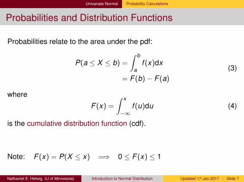
Probabilities and Distribution Functions

Probabilities relate to the area under the pdf:

P(a ≤ X ≤ b) =

∫ b

af (x)dx

= F (b)− F (a)

(3)

where

F (x) =

∫ x

−∞f (u)du (4)

is the cumulative distribution function (cdf).

Note: F (x) = P(X ≤ x) =⇒ 0 ≤ F (x) ≤ 1



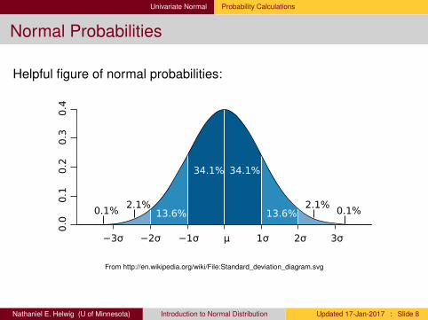
Normal Probabilities

Helpful figure of normal probabilities:0.0

0.1

0.2

0.3

0.4

−2σ −1σ 1σ−3σ 3σµ 2σ

34.1% 34.1%

13.6%2.1%

13.6% 0.1%0.1%2.1%

From http://en.wikipedia.org/wiki/File:Standard_deviation_diagram.svg



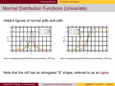
Normal Distribution Functions (Univariate)

Helpful figures of normal pdfs and cdfs:

- 3 - 2 - 1φ μ,σ

2(

0.8

0.6

0.4

0.2

0.0

−5 −3 1 3 5

x

1.0

−1 0 2 4−2−4

x)

0,μ=0,μ=0,μ=−2,μ=

2 0.2,σ =2 1.0,σ =2 5.0,σ =2 0.5,σ =

- 3 - 2 - 1

x

0.8

0.6

0.4

0.2

0.0

1.0

−5 −3 1 3 5−1 0 2 4−2−4

Φμ,σ2(x)

0,μ=0,μ=0,μ=−2,μ=

2 0.2,σ =2 1.0,σ =2 5.0,σ =2 0.5,σ =

http://en.wikipedia.org/wiki/File:Normal_Distribution_PDF.svg http://en.wikipedia.org/wiki/File:Normal_Distribution_CDF.svg

Note that the cdf has an elongated “S” shape, referred to as an ogive.


Univariate Normal Affine Transformations

Affine Transformations of Normal (Univariate)

Suppose that X ∼ N(µ, σ2) and a,b ∈ R with a 6= 0.

If we define Y = aX + b, then Y ∼ N(aµ+ b,a2σ2).

Suppose that X ∼ N(1,2). Determine the distributions of. . .Y = X + 3Y = 2X + 3Y = 3X + 2


Univariate Normal Affine Transformations

Affine Transformations of Normal (Univariate)

Suppose that X ∼ N(µ, σ2) and a,b ∈ R with a 6= 0.

If we define Y = aX + b, then Y ∼ N(aµ+ b,a2σ2).

Suppose that X ∼ N(1,2). Determine the distributions of. . .Y = X + 3 =⇒ Y ∼ N(1(1) + 3,12(2)) ≡ N(4,2)

Y = 2X + 3 =⇒ Y ∼ N(2(1) + 3,22(2)) ≡ N(5,8)

Y = 3X + 2 =⇒ Y ∼ N(3(1) + 2,32(2)) ≡ N(5,18)


Univariate Normal Parameter Estimation

Likelihood Function

Suppose that x = (x1, . . . , xn) is an iid sample of data from a normaldistribution with mean µ and variance σ2, i.e., xi

iid∼ N(µ, σ2).

The likelihood function for the parameters (given the data) has the form

L(µ, σ2|x) =n∏

i=1

f (xi) =n∏

i=1

1√2πσ2

exp{−(xi − µ)2

2σ2

}and the log-likelihood function is given by

LL(µ, σ2|x) =n∑

i=1

log(f (xi)) = −n2

log(2π)− n2

log(σ2)− 12σ2

n∑i=1

(xi−µ)2



Maximum Likelihood Estimate of the Mean

The MLE of the mean is the value of µ that minimizes

n∑i=1

(xi − µ)2 =n∑

i=1

x2i − 2nx̄µ+ nµ2

where x̄ = (1/n)∑n

i=1 xi is the sample mean.

Taking the derivative with respect to µ we find that

∂∑n

i=1(xi − µ)2

∂µ= −2nx̄ + 2nµ ←→ x̄ = µ̂

i.e., the sample mean x̄ is the MLE of the population mean µ.



Maximum Likelihood Estimate of the Variance

The MLE of the variance is the value of σ2 that minimizes

n2

log(σ2) +1

2σ2

n∑i=1

(xi − µ̂)2 =n2

log(σ2) +

∑ni=1 x2

i2σ2 − nx̄2

2σ2



Taking the derivative with respect to σ2 we find that

∂ n2 log(σ2) + 1

2σ2

∑ni=1(xi − µ̂)2

∂σ2 =n

2σ2 −1

2σ4

n∑i=1

(xi − µ̂)2

which implies that the sample variance σ̂2 = (1/n)∑n

i=1(xi − x̄)2 is theMLE of the population variance σ2.


Bivariate Normal

Bivariate Normal


Bivariate Normal Distribution Form

Normal Density Function (Bivariate)

Given two variables x , y ∈ R, the bivariate normal pdf is

f (x , y) =exp

{− 1

2(1−ρ2)

[(x−µx )2

σ2x

+(y−µy )2

σ2y− 2ρ(x−µx )(y−µy )

σxσy

]}2πσxσy

√1− ρ2

(5)

whereµx ∈ R and µy ∈ R are the marginal meansσx ∈ R+ and σy ∈ R+ are the marginal standard deviations0 ≤ |ρ| < 1 is the correlation coefficient

X and Y are marginally normal: X ∼ N(µx , σ2x ) and Y ∼ N(µy , σ

2y )



Example: µx = µy = 0, σ2x = 1, σ2

y = 2, ρ = 0.6/√

2

−4−2

02

4−4

−2

0

2

40.02

0.04

0.06

0.08

0.10

0.12

x

y

f(x, y

)

0.00

0.02

0.04

0.06

0.08

0.10

0.12

f(x, y

)

−4 −2 0 2 4

−4

−2

02

4

x

y

http://en.wikipedia.org/wiki/File:MultivariateNormal.png



Example: Different Means

0.00

0.02

0.04

0.06

0.08

0.10

0.12

f(x, y

)

−4 −2 0 2 4

−4

−2

02

4

µx = 0, µy = 0

x

y

0.00

0.02

0.04

0.06

0.08

0.10

0.12

f(x, y

)

−4 −2 0 2 4

−4

−2

02

4

µx = 1, µy = 2

x

y

0.00

0.02

0.04

0.06

0.08

0.10

0.12

f(x, y

)

−4 −2 0 2 4

−4

−2

02

4

µx = −1, µy = −1

x

y

Note: for all three plots σ2x = 1, σ2

y = 2, and ρ = 0.6/√

2.



Example: Different Correlations

0.00

0.02

0.04

0.06

0.08

0.10

0.12

f(x, y

)

−4 −2 0 2 4

−4

−2

02

4

ρ = −0.6/ 2

x

y

0.00

0.02

0.04

0.06

0.08

0.10

f(x, y

)

−4 −2 0 2 4

−4

−2

02

4

ρ = 0

x

y

0.00

0.05

0.10

0.15

0.20

f(x, y

)

−4 −2 0 2 4

−4

−2

02

4

ρ = 1.2/ 2

x

y

Note: for all three plots µx = µy = 0, σ2x = 1, and σ2

y = 2.



Example: Different Variances

0.00

0.05

0.10

0.15

f(x, y

)

−4 −2 0 2 4

−4

−2

02

4

σy = 1

x

y

0.00

0.02

0.04

0.06

0.08

0.10

0.12

f(x, y

)

−4 −2 0 2 4

−4

−2

02

4

σy = 2

x

y

0.00

0.02

0.04

0.06

0.08

f(x, y

)

−4 −2 0 2 4

−4

−2

02

4

σy = 2

x

y

Note: for all three plots µx = µy = 0, σ2x = 1, and ρ = 0.6/(σxσy ).


Bivariate Normal Probability Calculations

Probabilities and Multiple Integration

Probabilities still relate to the area under the pdf:

P([ax ≤ X ≤ bx ] and [ay ≤ Y ≤ by ]) =

∫ bx

ax

∫ by

ay

f (x , y)dydx (6)

where∫ ∫

f (x , y)dydx denotes the multiple integral of the pdf f (x , y).

Defining z = (x , y), we can still define the cdf:

F (z) = P(X ≤ x and Y ≤ y)

=

∫ x

−∞

∫ y

−∞f (u, v)dvdu

(7)


Bivariate Normal Probability Calculations

Normal Distribution Functions (Bivariate)

Helpful figures of bivariate normal pdf and cdf:

0.00

0.02

0.04

0.06

0.08

0.10

0.12

f(x, y

)

−4 −2 0 2 4

−4

−2

02

4

x

y

0.0

0.2

0.4

0.6

0.8

1.0

F(x

, y)

−4 −2 0 2 4

−4

−2

02

4

x

yNote: µx = µy = 0, σ2

x = 1, σ2y = 2, and ρ = 0.6/

√2

Note that the cdf still has an ogive shape (now in two-dimensions).Nathaniel E. Helwig (U of Minnesota) Introduction to Normal Distribution Updated 17-Jan-2017 : Slide 21

Bivariate Normal Affine Transformations

Affine Transformations of Normal (Bivariate)

Given z = (x , y)′, suppose that z ∼ N(µ,Σ) whereµ = (µx , µy )′ is the 2× 1 mean vector

Σ =

(σ2

x ρσxσyρσxσy σ2

y

)is the 2× 2 covariance matrix

Let A =

(a11 a12a21 a22

)and b =

(b1b2

)with A 6= 02×2 =

(0 00 0

).

If we define w = Az + b, then w ∼ N(Aµ + b,AΣA′).


Bivariate Normal Conditional Distributions

Conditional Normal (Bivariate)

The conditional distribution of a variable Y given X = x is

fY |X (y |X = x) =fXY (x , y)

fX (x)(8)

wherefXY (x , y) is the joint pdf of X and YfX (x) is the marginal pdf of X

In the bivariate normal case, we have that

Y |X ∼ N(µ∗, σ2∗) (9)

where µ∗ = µy + ρσyσx

(x − µx ) and σ2∗ = σ2

y (1− ρ2)



Derivation of Conditional Normal

To prove Equation (9), simply write out the definition and simplify:

fY |X (y|X = x) =fXY (x, y)

fX (x)

=

exp

{− 1

2(1−ρ2)

[(x−µx )2

σ2x

+(y−µy )2


σx σy

]}/(

2πσxσy√

1− ρ2)

exp{− (x−µx )2

2σ2x

}/(σx√

2π)

=

exp

{− 1

2(1−ρ2)

[(x−µx )2

σ2x

+(y−µy )2


σx σy

]+

(x−µx )2

2σ2x

}√

2πσy√

1− ρ2

=

exp

{− 1

2σ2y (1−ρ2)

[ρ2 σ2

yσ2

x(x − µx )

2 + (y − µy )2 − 2ρ

σyσx

(x − µx )(y − µy )

]}√

2πσy√

1− ρ2

=

exp

{− 1

2σ2y (1−ρ2)

[y − µy − ρ

σyσx

(x − µx )]2}

√2πσy

√1− ρ2

which completes the proof.



Statistical Independence for Bivariate Normal

Two variables X and Y are statistically independent if

fXY (x , y) = fX (x)fY (y) (10)

where fXY (x , y) is joint pdf, and fX (x) and fY (y) are marginals pdfs.

Note that if X and Y are independent, then

fY |X (y |X = x) =fXY (x , y)

fX (x)=

fX (x)fY (y)

fX (x)= fY (y) (11)

so conditioning on X = x does not change the distribution of Y .

If X and Y are bivariate normal, what is the necessary and sufficientcondition for X and Y to be independent? Hint: see Equation (9)Nathaniel E. Helwig (U of Minnesota) Introduction to Normal Distribution Updated 17-Jan-2017 : Slide 25


Example #1

A statistics class takes two exams X (Exam 1) and Y (Exam 2) wherethe scores follow a bivariate normal distribution with parameters:

µx = 70 and µy = 60 are the marginal meansσx = 10 and σy = 15 are the marginal standard deviationsρ = 0.6 is the correlation coefficient

Suppose we select a student at random. What is the probability that. . .(a) the student scores over 75 on Exam 2?(b) the student scores over 75 on Exam 2, given that the student

scored X = 80 on Exam 1?(c) the sum of his/her Exam 1 and Exam 2 scores is over 150?(d) the student did better on Exam 1 than Exam 2?(e) P(5X − 4Y > 150)?



Example #1: Part (a)

Answer for 1(a):Note that Y ∼ N(60,152), so the probability that the student scoresover 75 on Exam 2 is

P(Y > 75) = P(

Z >75− 60

15

)= P(Z > 1)

= 1− P(Z < 1)

= 1− Φ(1)

= 1− 0.8413447= 0.1586553

where Φ(x) =∫ x−∞ f (z)dz with f (x) = 1√

2πe−x2/2 denoting the standard

normal pdf (see R code for use of pnorm to calculate this quantity).



Example #1: Part (b)

Answer for 1(b):Note that (Y |X = 80) ∼ N(µ∗, σ

2∗) where

µ∗ = µY + ρσYσX

(x − µX ) = 60 + (0.6)(15/10)(80− 70) = 69σ2∗ = σ2

Y (1− ρ2) = 152(1− 0.62) = 144

If a student scored X = 80 on Exam 1, the probability that the studentscores over 75 on Exam 2 is

P(Y > 75|X = 80) = P(

Z >75− 69

12

)= P (Z > 0.5)

= 1− Φ(0.5)

= 1− 0.6914625= 0.3085375



Example #1: Part (c)

Answer for 1(c):Note that (X + Y ) ∼ N(µ∗, σ

2∗) where

µ∗ = µX + µY = 70 + 60 = 130σ2∗ = σ2

X + σ2Y + 2ρσXσY = 102 + 152 + 2(0.6)(10)(15) = 505

The probability that the sum of Exam 1 and Exam 2 is above 150 is

P(X + Y > 150) = P(

Z >150− 130√

505

)= P (Z > 0.8899883)

= 1− Φ(0.8899883)

= 1− 0.8132639= 0.1867361



Example #1: Part (d)

Answer for 1(d):Note that (X − Y ) ∼ N(µ∗, σ

2∗) where

µ∗ = µX − µY = 70− 60 = 10σ2∗ = σ2

X + σ2Y − 2ρσXσY = 102 + 152 − 2(0.6)(10)(15) = 145

The probability that the student did better on Exam 1 than Exam 2 is

P(X > Y ) = P(X − Y > 0)

= P(

Z >0− 10√

145

)= P (Z > −0.8304548)

= 1− Φ(−0.8304548)

= 1− 0.2031408= 0.7968592



Example #1: Part (e)

Answer for 1(e):Note that (5X − 4Y ) ∼ N(µ∗, σ

2∗) where

µ∗ = 5µX − 4µY = 5(70)− 4(60) = 110σ2∗ = 52σ2

X + (−4)2σ2Y + 2(5)(−4)ρσXσY =

25(102) + 16(152)− 2(20)(0.6)(10)(15) = 2500

Thus, the needed probability can be obtained using

P(5X − 4Y > 150) = P(

Z >150− 110√

2500

)= P (Z > 0.8)

= 1− Φ(0.8)

= 1− 0.7881446= 0.2118554



Example #1: R Code

# Example 1a> pnorm(1,lower=F)[1] 0.1586553> pnorm(75,mean=60,sd=15,lower=F)[1] 0.1586553

# Example 1b> pnorm(0.5,lower=F)[1] 0.3085375> pnorm(75,mean=69,sd=12,lower=F)[1] 0.3085375

# Example 1c> pnorm(20/sqrt(505),lower=F)[1] 0.1867361> pnorm(150,mean=130,sd=sqrt(505),lower=F)[1] 0.1867361

# Example 1d> pnorm(-10/sqrt(145),lower=F)[1] 0.7968592> pnorm(0,mean=10,sd=sqrt(145),lower=F)[1] 0.7968592

# Example 1e> pnorm(0.8,lower=F)[1] 0.2118554> pnorm(150,mean=110,sd=50,lower=F)[1] 0.2118554


Multivariate Normal

Multivariate Normal


Multivariate Normal Distribution Form

Normal Density Function (Multivariate)

Given x = (x1, . . . , xp)′ with xj ∈ R ∀j , the multivariate normal pdf is

f (x) =1

(2π)p/2|Σ|1/2 exp{−1

2(x− µ)′Σ−1(x− µ)

}(12)

whereµ = (µ1, . . . , µp)′ is the p × 1 mean vector

Σ =

σ11 σ12 · · · σ1pσ21 σ22 · · · σ2p

......

. . ....

σp1 σp2 · · · σpp

is the p × p covariance matrix

Write x ∼ N(µ,Σ) or x ∼ Np(µ,Σ) to denote x is multivariate normal.


Multivariate Normal Distribution Form

Some Multivariate Normal Properties

The mean and covariance parameters have the following restrictions:µj ∈ R for all jσjj > 0 for all jσij = ρij

√σiiσjj where ρij is correlation between Xi and Xj

σ2ij ≤ σiiσjj for any i , j ∈ {1, . . . ,p} (Cauchy-Schwarz)

Σ is assumed to be positive definite so that Σ−1 exists.

Marginals are normal: Xj ∼ N(µj , σjj) for all j ∈ {1, . . . ,p}.


Multivariate Normal Probability Calculations

Multivariate Normal Probabilities

Probabilities still relate to the area under the pdf:

P(aj ≤ Xj ≤ bj ∀j) =

∫ b1

a1

· · ·∫ bp

ap

f (x)dxp · · · dx1 (13)

where∫· · ·∫

f (x)dxp · · · dx1 denotes the multiple integral f (x).

We can still define the cdf of x = (x1, . . . , xp)′

F (x) = P(Xj ≤ xj ∀j)

=

∫ x1

−∞· · ·∫ xp

−∞f (u)dup · · · du1

(14)


Multivariate Normal Affine Transformations

Affine Transformations of Normal (Multivariate)

Suppose that x = (x1, . . . , xp)′ and that x ∼ N(µ,Σ) whereµ = {µj}p×1 is the mean vectorΣ = {σij}p×p is the covariance matrix

Let A = {aij}n×p and b = {bi}n×1 with A 6= 0n×p.

If we define w = Ax + b, then w ∼ N(Aµ + b,AΣA′).

Note: linear combinations of normal variables are normally distributed.


Multivariate Normal Conditional Distributions

Multivariate Conditional Distributions

Given variables x = (x1, . . . , xp)′ and y = (y1, . . . , yq)′, we have

fY |X (y|X = x) =fXY (x,y)

fX (x)(15)

wherefY |X (y|X = x) is the conditional distribution of y given xfXY (x,y) is the joint pdf of x and yfX (x) is the marginal pdf of x



Conditional Normal (Multivariate)

Suppose that z ∼ N(µ,Σ) wherez = (x′,y′)′ = (x1, . . . , xp, y1, . . . , yq)′

µ = (µ′x ,µ′y )′ = (µ1x , . . . , µpx , µ1y , . . . , µqy )′

Note: µx is mean vector of x, and µy is mean vector of y

Σ =

(Σxx ΣxyΣ′xy Σyy

)where (Σxx )p×p, (Σyy )q×q, and (Σxy )p×q,

Note: Σxx is covariance matrix of x, Σyy is covariance matrix of y,and Σxy is covariance matrix of x and y

In the multivariate normal case, we have that

y|x ∼ N(µ∗,Σ∗) (16)

where µ∗ = µy + Σ′xyΣ−1xx (x− µx ) and Σ∗ = Σyy −Σ′xyΣ

−1xx Σxy



Statistical Independence for Multivariate Normal

Using Equation (16), we have that

y|x ∼ N(µ∗,Σ∗) ≡ N(µy ,Σyy ) (17)

if and only if Σxy = 0p×q (a matrix of zeros).

Note that Σxy = 0p×q implies that the p elements of x are uncorrelatedwith the q elements of y.

For multivariate normal variables: uncorrelated→ independentFor non-normal variables: uncorrelated 6→ independent



Example #2

Each Delicious Candy Company store makes 3 size candy bars:regular (X1), fun size (X2), and big size (X3).

Assume the weight (in ounces) of the candy bars (X1,X2,X3) follow amultivariate normal distribution with parameters:

µ =

537

and Σ =

4 −1 0−1 4 20 2 9

Suppose we select a store at random. What is the probability that. . .(a) the weight of a regular candy bar is greater than 8 oz?(b) the weight of a regular candy bar is greater than 8 oz, given that

the fun size bar weighs 1 oz and the big size bar weighs 10 oz?(c) P(4X1 − 3X2 + 5X3 < 63)?



Example #2: Part (a)

Answer for 2(a):Note that X1 ∼ N(5,4)

So, the probability that the regular bar is more than 8 oz is

P(X1 > 8) = P(

Z >8− 5

2

)= P(Z > 1.5)

= 1− Φ(1.5)

= 1− 0.9331928= 0.0668072



Example #2: Part (b)

Answer for 2(b):(X1|X2 = 1,X3 = 10) is normally distributed, see Equation (16).

The conditional mean of (X1|X2 = 1,X3 = 10) is given by

µ∗ = µX1 + Σ′12Σ−122 (x̃− µ̃)

= 5 +(−1 0

)(4 22 9

)−1( 1− 310− 7

)= 5 +

(−1 0

) 132

(9 −2−2 4

)(−23

)= 5 + 24/32= 5.75



Example #2: Part (b) continued

Answer for 2(b) continued:The conditional variance of (X1|X2 = 1,X3 = 10) is given by

σ2∗ = σ2

X1−Σ′12Σ

−122 Σ12

= 4−(−1 0

)(4 22 9

)−1(−10

)= 4−

(−1 0

) 132

(9 −2−2 4

)(−10

)= 4− 9/32= 3.71875



Example #2: Part (b) continued

Answer for 2(b) continued:So, if the fun size bar weighs 1 oz and the big size bar weighs 10 oz,the probability that the regular bar is more than 8 oz is

P(X1 > 8|X2 = 1,X3 = 10) = P(

Z >8− 5.75√3.71875

)= P(Z > 1.166767)

= 1− Φ(1.166767)

= 1− 0.8783477= 0.1216523



Example #2: Part (c)

Answer for 2(c):(4X1 − 3X2 + 5X3) is normally distributed.

The expectation of (4X1 − 3X2 + 5X3) is given by

µ∗ = 4µX1 − 3µX2 + 5µX3

= 4(5)− 3(3) + 5(7)

= 46



Example #2: Part (c) continued

Answer for 2(c) continued:The variance of (4X1 − 3X2 + 5X3) is given by

σ2∗ =

(4 −3 5

)Σ

4−35

=(4 −3 5

) 4 −1 0−1 4 20 2 9

4−35

=(4 −3 5

)19−639

= 289



Example #2: Part (c) continued

Answer for 2(c) continued:So, the needed probability can be obtained as

P(4X1 − 3X2 + 5X3 < 63) = P(

Z <63− 46√

289

)= P(Z < 1)

= Φ(1)

= 0.8413447



Example #2: R Code

# Example 2a> pnorm(1.5,lower=F)[1] 0.0668072> pnorm(8,mean=5,sd=2,lower=F)[1] 0.0668072

# Example 2b> pnorm(2.25/sqrt(119/32),lower=F)[1] 0.1216523> pnorm(8,mean=5.75,sd=sqrt(119/32),lower=F)[1] 0.1216523

# Example 2c> pnorm(1)[1] 0.8413447> pnorm(63,mean=46,sd=17)[1] 0.8413447


Multivariate Normal Parameter Estimation

Likelihood Function

Suppose that xi = (xi1, . . . , xip) is a sample from a normal distribution

with mean vector µ and covariance matrix Σ, i.e., xiiid∼ N(µ,Σ).

The likelihood function for the parameters (given the data) has the form

L(µ,Σ|X) =n∏

i=1

f (xi) =n∏

i=1

1(2π)p/2|Σ|1/2 exp

{−1

2(xi − µ)′Σ−1(xi − µ)

}and the log-likelihood function is given by

LL(µ,Σ|X) = −np2

log(2π)− n2

log(|Σ|)− 12

n∑i=1

(xi − µ)′Σ−1(xi − µ)



Maximum Likelihood Estimate of Mean Vector

The MLE of the mean vector is the value of µ that minimizes

n∑i=1

(xi − µ)′Σ−1(xi − µ) =n∑

i=1

x′iΣ−1xi − 2nx̄′Σ−1µ + nµ′Σ−1µ


i=1 xi is the sample mean vector.

Taking the derivative with respect to µ we find that

∂LL(µ,Σ|X)

∂µ= −2nΣ−1x̄ + 2nΣ−1µ ←→ x̄ = µ̂

The sample mean vector x̄ is the MLE of the population mean µ vector.



Maximum Likelihood Estimate of Covariance Matrix

The MLE of the covariance matrix is the value of Σ that minimizes

−n log(|Σ−1|) +n∑

i=1

tr{Σ−1(xi − µ̂)(xi − µ̂)′}

where µ̂ = x̄ = (1/n)∑n


Taking the derivative with respect to Σ−1 we find that

∂LL(µ,Σ|X)

∂Σ−1 = −nΣ +n∑

i=1

(xi − µ̂)(xi − µ̂)′

i.e., the sample covariance matrix Σ̂ = (1/n)∑n

i=1(xi − x̄)(xi − x̄)′ isthe MLE of the population covariance matrix Σ.


Sampling Distributions

Sampling Distributions


Sampling Distributions Univariate Case

Univariate Sampling Distributions: x̄ and s2

In the univariate normal case, we have thatx̄ = (1/n)

∑ni=1 xi ∼ N(µ, σ2/n)

(n − 1)s2 =∑n

i=1(xi − x̄)2 ∼ σ2χ2n−1

χ2k denotes a chi-square variable with k degrees of freedom.

σ2χ2k =

∑ki=1 z2

i where ziiid∼ N(0, σ2)


Sampling Distributions Multivariate Case

Multivariate Sampling Distributions: x̄ and S

In the multivariate normal case, we have thatx̄ = (1/n)

∑ni=1 xi ∼ N(µ,Σ/n)

(n − 1)S =∑n

i=1(xi − x̄)(xi − x̄)′ ∼Wn−1(Σ)

Wk (Σ) denotes a Wishart variable with k degrees of freedom.

Wk (Σ) =∑k

i=1 ziz′i where ziiid∼ N(0p,Σ)


Nathaniel E. Helwig - School of Statistics : University of...

Documents

Transcript of Nathaniel E. Helwig - School of Statistics : University of...