Septem

NASA/

PilotComBoom Sanford FFidell As Richard DConsulta Michael HFidell As

mber 2012

/CR–2012

t Test ommunit

ms

Fidell ssociates, Inc

D. Horonjeffant, Boxboro

Harris ssociates, Inc

2

2-217767

of a Nty Resp

c., Woodland

ff ugh, Massac

c., Woodland

Novel Mponse

d Hills, Calif

chusetts

d Hills, Calif

Methodto Low

ifornia

ifornia

d for Aw-Am

Assessmplitud

sing de Soniic

https://ntrs.nasa.gov/search.jsp?R=20120014937 2019-12-28T17:15:16+00:00Z

NASA STI Program . . . in Profile

Since its founding, NASA has been dedicated to the advancement of aeronautics and space science. The NASA scientific and technical information (STI) program plays a key part in helping NASA maintain this important role.

The NASA STI program operates under the auspices of the Agency Chief Information Officer. It collects, organizes, provides for archiving, and disseminates NASA’s STI. The NASA STI program provides access to the NASA Aeronautics and Space Database and its public interface, the NASA Technical Report Server, thus providing one of the largest collections of aeronautical and space science STI in the world. Results are published in both non-NASA channels and by NASA in the NASA STI Report Series, which includes the following report types:

TECHNICAL PUBLICATION. Reports of

completed research or a major significant phase of research that present the results of NASA Programs and include extensive data or theoretical analysis. Includes compilations of significant scientific and technical data and information deemed to be of continuing reference value. NASA counterpart of peer-reviewed formal professional papers, but having less stringent limitations on manuscript length and extent of graphic presentations.

TECHNICAL MEMORANDUM. Scientific

and technical findings that are preliminary or of specialized interest, e.g., quick release reports, working papers, and bibliographies that contain minimal annotation. Does not contain extensive analysis.

CONTRACTOR REPORT. Scientific and

technical findings by NASA-sponsored contractors and grantees.

CONFERENCE PUBLICATION.

Collected papers from scientific and technical conferences, symposia, seminars, or other meetings sponsored or co-sponsored by NASA.

SPECIAL PUBLICATION. Scientific,

technical, or historical information from NASA programs, projects, and missions, often concerned with subjects having substantial public interest.

TECHNICAL TRANSLATION.

English-language translations of foreign scientific and technical material pertinent to NASA’s mission.

Specialized services also include organizing and publishing research results, distributing specialized research announcements and feeds, providing information desk and personal search support, and enabling data exchange services. For more information about the NASA STI program, see the following: Access the NASA STI program home page

at http://www.sti.nasa.gov E-mail your question to help@sti.nasa.gov Fax your question to the NASA STI

Information Desk at 443-757-5803 Phone the NASA STI Information Desk at

443-757-5802 Write to:

STI Information Desk NASA Center for AeroSpace Information 7115 Standard Drive Hanover, MD 21076-1320

National ASpace Adm Langley RHampton

Septem

NASA/

PilotComBoom Sanford FFidell As Richard DConsulta Michael HFidell As

Aeronautics aministration

Research Centn, Virginia 236

mber 2012

/CR–2012

t Test ommunit

ms

Fidell ssociates, Inc

D. Horonjeffant, Boxboro

Harris ssociates, Inc

and

ter 681-2199

2

2-217767

of a Nty Resp

c., Woodland

ff ugh, Massac

c., Woodland

Novel Mponse

d Hills, Calif

chusetts

d Hills, Calif

Pu

Methodto Low

ifornia

ifornia

Prepared for under Contra

d for Aw-Am

Langley Reseact NNL10AA

Assessmplitud

earch Center A19C

sing de Soniic

Available from:

NASA Center for AeroSpace Information 7115 Standard Drive

Hanover, MD 21076-1320 443-757-5802

The use of trademarks or names of manufacturers in this report is for accurate reporting and does not constitute an official endorsement, either expressed or implied, of such products or manufacturers by the National Aeronautics and Space Administration.

3

Table of Contents

1 SUMMARY ............................................................................................................................... 81.1 Purpose and Organization of Report .......................................................................................... 81.2 Background ................................................................................................................................ 81.3 General findings about immediate reactions to booms ............................................................ 101.4 General findings about entire-day reactions to booms ............................................................. 101.5 Findings about compliance with instructions for smartphone use............................................ 101.6 Response latencies and interview durations for immediate response interviews ..................... 101.7 Ease of use of smartphones ...................................................................................................... 11

2 STUDY DESIGN ..................................................................................................................... 122.1 Nature of test participant sample.............................................................................................. 122.2 Types of interviews administered by smartphone .................................................................... 122.3 Distribution of smartphones to test participants ....................................................................... 19

3 PRIMARY FINDINGS ............................................................................................................ 203.1 Estimation of sonic boom exposure levels ............................................................................... 203.2 Distributions of levels of individual sonic booms noticed by test participants ........................ 223.3 Relationship among metrics of estimated sonic boom exposure levels ................................... 223.4 Interpretability of findings of end-of-day interview data 95.3 ................................................. 233.5 Demonstration of analyzability of immediate response interview data.................................... 243.6 Development of formal dosage-response relationships............................................................ 25

4 DISCUSSION OF METHODOLOGICAL FINDINGS .......................................................... 284.1 Reports of notice of individual sonic booms (immediate responses) ....................................... 284.2 Response latencies and interview durations ............................................................................. 284.3 Opinions about cumulative exposure to sonic booms (end-of-day interviews) ....................... 294.4 Debriefing interviews ............................................................................................................... 314.5 Adequacy of recruitment incentives......................................................................................... 31

5 DISCUSSION OF SUBSTANTIVE FINDINGS..................................................................... 325.1 Estimation of cumulative exposure to sonic booms ................................................................. 325.2 Dosage-response analyses of current findings.......................................................................... 345.3 Comparisons of dosage-response relationship for end-of-day interview reports of annoyancewith prior findings................................................................................................................................... 37

6 LESSONS LEARNED ............................................................................................................. 406.1 Recommendations about scheduling of intentional exposures to sonic booms........................ 406.2 Recommendation for extension of scale of application of technique....................................... 426.3 Porting of application code to iOS (Apple) devices ................................................................. 436.4 Improvements to participant instructions ................................................................................. 446.5 Minor improvements to features of smartphone reporting application .................................... 456.6 Measures useful for estimating exposure levels over a wide area............................................ 45

7 CONCLUSIONS ...................................................................................................................... 47

8 ACKNOWLEDGMENTS........................................................................................................ 48

4

9 REFERENCES......................................................................................................................... 49

10 APPENDIX A: WRITTEN INSTRUCTIONS TO TEST PARTICIPANTS.......................... 50

11 APPENDIX B: ILLUSTRATIONS OF SECONDARY ANALYSES OF SMARTPHONE-COLLECTED INTERVIEW DATA.......................................................................................................... 52

11.1 Response patterns to sonic booms............................................................................................ 5211.2 Response latencies and implications ........................................................................................ 5611.3 Low battery conditions encountered by test participants ......................................................... 5711.4 Percentages of test participants at home during day and nighttime periods............................. 5811.5 Questionnaire completion rates ................................................................................................ 5911.6 Reports of notice of individual sonic boom events as functions of sound levels ..................... 6111.7 Analysis of responses to question about individually memorable booms................................ 6411.8 Reports of annoyance of individual sonic boom events as functions of sound levels.............. 6711.9 Reports of startle associated with individual sonic boom events as functions of sound levels 68

5

List of Tables

Table 1: Frequency of self-reported response latency ............................................................................... 11Table 2: Locations of test participants when they reported individual sonic booms ................................. 28Table 3: Numbers of test participants completing end-of-day interviews on each day of intentional

booming period ................................................................................................................................... 30Table 4: Comparison of variously estimated CDNL values and percentages of annoyance reports in

varying degrees ................................................................................................................................... 33

6

List of Figures

Figure 1: Default home screen of government-furnished smartphone, intended to minimize effortrequired to report notice of a sonic boom. .......................................................................................... 13

Figure 2: Appearance of screen displaying initial questionnaire item. [Q1] ............................................ 14Figure 3: Appearance of screen displaying screening item for annoyance judgment. (A “No” response

skips the next questionnaire item.) [Q2] ............................................................................................ 14Figure 4: Appearance of screen displaying response alternatives for questionnaire item soliciting an

annoyance rating. [Q3]....................................................................................................................... 15Figure 5: Appearance of screen for initial questionnaire item concerning startle. [Q4] ........................... 15Figure 6: Appearance of screen for questionnaire item inquiring about location of test participant at time

of notice of a sonic boom. [Q5] ......................................................................................................... 16Figure 7: Appearance of screen for questionnaire item inquiring about notice of rattling sounds. (A “No”

response skips the next item.) [Q6].................................................................................................... 16Figure 8: Appearance of screen for questionnaire item inquiring about annoyance of rattling sounds. (A

“No” response skips the next item.) [Q7] .......................................................................................... 17Figure 9: Appearance of screen for questionnaire item inquiring about degree of annoyance of rattling

sounds. [Q8]....................................................................................................................................... 17Figure 10: Appearance of screen thanking test participants for reporting a sonic boom........................... 18Figure 11: Exposure surface for a single sonic boom, calculated by short range geo-interpolation of

sound level measurements made at thirteen monitoring points. ......................................................... 21Figure 12: Illustration of interpretability of end-of-day annoyance judgments. ........................................ 23Figure 13: Illustration of interpretability of reports of notice and annoyance in immediate (single event)

interviews............................................................................................................................................ 24Figure 14: Linear regression of percentage of at-home respondents highly annoyed by C-weighted sound

exposure levels estimated by two methods. ........................................................................................ 27Figure 15: Distribution of response latencies for reporting individual booms within the first fifteen

minutes (900 seconds) of their occurrence.......................................................................................... 29Figure 16: Distribution of durations of immediate response interviews.................................................... 30Figure 17: Percentages of test participants completing end-of-day interviews on each day of the

intentional booming period. ................................................................................................................ 31Figure 18: Comparison of relationship between high annoyance and mean CDNL values for each day of

intentional booming period as estimated by three methods. ............................................................... 34Figure 19: Fit of the current data to the annoyance prevalence rates predicted by CTL analysis.............. 35Figure 20: CTL-based relationships between variously defined degrees of annoyance and estimated

CDNL values ...................................................................................................................................... 36Figure 21: Similarity of current findings (filled red plotting symbols) to a prior determination (Borsky,

1965) of the prevalence of high annoyance with sonic booms. .......................................................... 38Figure 22: Comparison of current data (filled red plotting symbols) with prior observations cataloged by

Fidell (1996)........................................................................................................................................ 38Figure 23: Prevalence of annoyance with low-amplitude sonic booms (filled red plotting symbols) in

relation to similar findings of 44 other studies of the annoyance of aircraft noise (Fidell et al., 2011.)............................................................................................................................................................ 39

Figure 24: Chronology of sonic boom reports during participant possession of smartphones. ................. 52Figure 25: Time history of sonic boom responses for week 10/30/2011 through 11/05/2011. ................. 53Figure 26: Chronology of sonic boom responses for week 11/06/2011 through 11/12/2011.................... 54Figure 27: Chronology of sonic boom responses for week 11/13/2011 through 11/20/2011.................... 54Figure 28: Sonic boom response time history for 14 November 2011. ..................................................... 55

7

Figure 29: Response time history for a 1-1/2 hour period of intentional sonic booms on 31 August 2011............................................................................................................................................................. 55

Figure 30: Cumulative distribution function of observed response latencies as long as an hour following aboom. .................................................................................................................................................. 56

Figure 31: Cumulative distribution function of observed response latencies up to 15 minutes followingboom event.......................................................................................................................................... 57

Figure 32: Percentages of test participants encountering varying numbers of low battery conditions duringthe test period...................................................................................................................................... 58

Figure 33: Comparison of at-home status between daytime and evening/nighttime periods .................... 59Figure 34: Participant at-home status by hour of day, for weekday/weekend periods. ............................. 60Figure 35: Percentage of respondents answering questions on immediate response questionnaire (see

Figure 2 though Figure 9). .................................................................................................................. 61Figure 36: Percentages of at-home participants noticing sonic booms as a function of maximum boom

overpressure. ....................................................................................................................................... 62Figure 37: Percentages of at-home participants noticing sonic booms as a function of C-weighted sound

exposure level. .................................................................................................................................... 63Figure 38: Percentages of at-home participants noticing sonic booms as a function of maximum boom

overpressure (logarithmic scale) ......................................................................................................... 63Figure 39: Observed relationship between C-weighted sound exposure level and square of maximum

overpressure (dashed line is unity slope) ............................................................................................ 64Figure 40: Relationship between percent of respondents reporting one boom to be louder than all others

for the day and CDNL......................................................................................................................... 65Figure 41: Relationship between percent of respondents reporting one boom louder than others and CSEL

difference between loudest and next loudest boom. ........................................................................... 66Figure 42: Relationship between percent of respondents reporting one boom louder than others and CSEL

difference between loudest and next loudest boom (with fit line). ..................................................... 66Figure 43: Relationship between percent of respondents reporting one boom to be louder than all others

for the day and the difference in CDNLs between that of the loudest boom and all the rest (with fitline). .................................................................................................................................................... 67

Figure 44: Percentages of at-home test participants reporting three different degrees of annoyance tosonic booms as a function of C-weighted sound exposure level......................................................... 68

Figure 45: Percentages of at-home test participants reporting startle to sonic booms as a function of C-weighted sound exposure level. .......................................................................................................... 69

Figure 46: Percentages of at-home test participants noticing rattle as a function of C-weighted soundexposure level. .................................................................................................................................... 69

8

1 SUMMARY

1.1 Purpose and Organization of Report

This document is the final technical report for NASA Contract NNL10AA19C. It describes apilot test of a novel method for assessing the annoyance of residential exposure to sonic booms.The report presents information about data collection methods and about test participants’reactions to low-amplitude sonic booms. The latter information should not be viewed asdefinitive for several reasons. It may not be reliably generalized to the wider U.S. residentialpopulation (because it was not derived from a representative random sample); the sample itselfwas not large; and the uncertainty of acoustic measurements of the exposure of test participantsto sonic booms is difficult to quantify.

Following a brief overview of findings in this section, a Study Design section providesfurther information about study methods. The report then presents details of primary findings,followed by discussion of the methodological and substantive results. A “Lessons Learned”discussion precedes Conclusions. Two appendices contain the instructions provided to testparticipants, and the findings of secondary analyses.

1.2 Background

The novel aspect of the current study is reliance on smartphones to collect near-real timeopinions about the annoyance of sonic booms. Many people customarily carry cell phones withthem as part of their daily routines.1 Smartphone-based interviews can thus be convenientlyconducted in close temporal proximity to the occurrence of sonic booms, not only whilerespondents are at home, but also while they are away from home. Questionnaires administeredby smartphone can improve the precision, immediacy, and cost-effectiveness of fieldassessments of community response to infrequent and unanticipated sonic booms. Because theuse of smartphones permits conduct of adaptive study designs, they can minimize the costs ofunnecessary community exposure to impulsive noise, while widening the range of analyses thatcan be practically conducted. Near real-time data collection, as well as the availability ofsituational information about the circumstances of interviewing, offer novel opportunities forfine-grained analyses of noise-induced annoyance.

Edwards Air Force Base was chosen as the venue for the current pilot study for theconvenience it affords in producing and measuring exposure and reactions to sonic boomsgenerated by aircraft based at NASA’s adjoining Dryden Research Center. Residents of this AirForce base also have long familiarity with sonic booms created by aircraft operations in a nearbysupersonic flight corridor. During the first two weeks of November, 2011, residents of the basehousing area at Edwards AFB were exposed to nearly 90 low amplitude sonic booms that wereintentionally produced by NASA flight operations. (They were also exposed both intentionallyand adventitiously to about 20 additional higher amplitude sonic booms during the same timeperiod.)

Motorola Droid2 smartphones were distributed to 49 test participants, mostly spouses ofmilitary personnel living at Edwards AFB, between August and October of 2012. The test

1 It was recently estimated that approximately half of U.S. households (about 60 million) have smartphone and/orother internet-enabled mobile devices.

9

participants were encouraged to use these government-supplied smartphones for their routinepersonal purposes, without charge, for the duration of the field study. They were also asked tocomplete two forms of interview. First, they were instructed to push a large red button on thehome screens of these smartphones, and to complete a brief interview administered viasmartphone, whenever they noticed a sonic boom at any time of night or day, whether at home orelsewhere. Second, they were instructed to answer several questions at the end of the dayconcerning their entire day’s reactions to sonic booms. The survey was administered by thesmartphone application, and required no connection to the database server.

Interview information collected by the smartphones was transmitted - without any testparticipant involvement, via wireless commercial digital network - to a remote, cloud-basedserver. The server created separate databases for responses to questionnaire items of theimmediate and end-of-day interviews. The smartphones reported basic “health” information(e.g., available memory, battery charge, at-home status, and network connectivity) to the serverfour times per hour. This information was transmitted to the server as soon as contact could beestablished, so that the status of smartphones could be archived regardless of server accessibilityor communication link status. The server’s password-protected databases were immediatelyavailable via the Internet to analysts to monitor the course of data collection, and for qualitycontrol-related purposes. Measures were taken to anonymize the identities of test participants topreclude disclosure of any personally-identifiable information.

Test participants made 2152 sonic boom reports during the two-week intentional boomingperiod. Of these, 1717 (79.8%) were reports made from home, where sound level doses couldreasonably be estimated. Of the 1717 at-home responses, 1631 (95.0%) were for indoorexposure to a boom. Since only 86 reports were received for the at-home/outdoor exposurecondition, no attempt was made to compare indoor versus outdoor levels of annoyance forsimilar boom intensities, nor did the outdoor reports contribute to individual event analyses.

Of the 1631 indoor/at-home reports, 1413 (86.6%) could be unambiguously linked to anestimated outdoor boom level. The remaining 218 (13.4%) could not be positively linked forreasons discussed later. The most common reason was an inter-boom interval shorter than aresponse latency.

The text of the following subsections focuses on the 1413 immediate reaction reports forwhich it was possible to unambiguously attribute opinions expressed in interviews to specificsonic booms while test participants were indoors at home during the two-week long intentionalbooming period. Note that denominators for sample proportions are not necessarily 49 (themaximum number of test participants who could potentially have filed reports), but are adjustedfor numbers of participants who were at home with charged smartphones at the times ofoccurrence of sonic booms.

Information about end-of-day interviews is analyzed at length in Section 5.3 on page 37 ofthis report.

10

1.3 General findings about immediate reactions to booms

The at-home, indoors responses indicated annoyance in some degree in 24% (338 of 1413) ofthe reports of notice of sonic booms during the intentional booming period2. These responsesfurther indicated “high” (“very” or “extremely”) annoyance in 5% (76 of 1413) of the cases.Test participants describe themselves as startled by booms in 29% (409 of 1413) of the reports.

Notice of rattle was reported in 48.6% (685 of 1413) of the cases. The mean of the peakoverpressures of booms for which test participants noticed rattle was 0.67 psf, while the mean ofthe peak overpressures of booms for which test participants did not report rattle was 0.45 psf.The difference in overpressures for booms that were and were not associated with notice of rattlewas unlikely to have arisen by chance alone (F(df = 1412) = 57.92, p < .0001).

As is evident from the discussion of Sections 3.4 through 3.6 and Section and 4.5, and fromthe illustrations in Appendix B, the intensity of reactions to booms generally increased withincreasing boom levels.

1.4 General findings about entire-day reactions to booms

Completion rates for interviews about test participants’ exposure to full days of sonic boomexposure were comparable to those usually obtained by conventional social survey techniques.The percentages of respondents describing themselves as highly annoyed by whole days ofexposure to sonic booms were well accounted for by the effective loudness of the exposure, asdescribed in greater detail in Section 5.2.

The percentages of test participants highly annoyed by exposure to low-amplitude sonicbooms closely resembled those measured by conventional social survey methods in OklahomaCity (Borsky, 1965). Greater percentages of test participants were highly annoyed by exposureto low-amplitude sonic booms than by exposure to conventional (sub-sonic) aircraft noise atsimilar cumulative exposure levels.

1.5 Findings about compliance with instructions for smartphone use

Compliance by the test participants with instructions to use their smartphones to report noticeof sonic booms was excellent. During the entire (August-November) period during which testparticipants were in possession of government-furnished smartphones, they reported noticing atotal of 157 distinct sonic booms. They collectively completed 3266 reports of notice ofindividual sonic booms during the two-week long intentional booming period. Of these, tenpercent of the test participants reported noticing 64% or more of all sonic booms. Twentypercent reported noticing 58% or more of the booms. Fifty percent of the participants reportednoticing 43% or more of the booms. The most common difficulty encountered by testparticipants in the use of smartphones was remembering to recharge them nightly.

1.6 Response latencies and interview durations for immediate response interviews

Test participants described the times of occurrence of sonic booms at the very beginning ofthe questionnaire (Item 1). They were instructed to select from one of the three categories shown

2 Note that the divisors for percentages in this subsection are the number of at-home respondents providing aninterview, not the total number of at-home participants (some of whom did not provide interviews).

11

in Table 1. Nearly 85% (2767 of 3266)3 reported the boom as occurring “within the last fewminutes.”4 (Section 2 of this report describes the individual questionnaire items to which testparticipants responded.) Actual response latencies (elapsed time between the occurrence of aboom and receipt of a report of noticing it) ranged from as little as 16 seconds to as long as 2hours after the occurrence of a sonic boom. The response latencies were exponentiallydistributed, with a mean latency of 276 seconds and a standard deviation of 871 seconds (cf.Figure 15 on page 29).

The distribution of interview durations for immediate reports of notice of sonic booms wasapproximately lognormal, with a mean duration of 17.3 seconds and a standard deviation of 12.8seconds (cf. Figure 16 on page 30).

Table 1: Frequency of self-reported response latency

Self-reported responselatency

Number Percent

Last Few Minutes 2767 84.7%

More Than Half Hour 248 7.6%

Last Hour 251 7.7%

Total 3266 100.0%

During the two-week period of intentional exposure to sonic booms, the test participants alsocompleted 377 interviews about their end-of-day reactions to sonic booms. In the severalmonths prior to the intentional booming period in November, 2011, the test participantscompleted an additional 2027 end-of-day interviews. The mean duration for the end-of-dayinterviews during the intentional booming period was 13.6 seconds.

1.7 Ease of use of smartphones

Test participants were provided with an automatic texting address and an automatically-dialable telephone hotline number that they could use to request live assistance in the use of theirsmartphones. Few respondents called to ask for such assistance, nor reported any difficulty inthe use of the smartphones distributed to them. Smartphones were charged and available for usemore than 91% of the time.

3 These numbers include all interviews while the smartphones were in the participants’ possession, not just duringthe intentional booming period.4 Not all of these interviews were usable in the dose-response relationships described later in this report, becausenot all could be unambiguously linked to a specific sonic boom.

12

2 STUDY DESIGN

2.1 Nature of test participant sample

NASA provided a purposive sample of 49 test participants in several batches, starting inearly August and concluding in mid-October of 2011. All were self-selected volunteers residingin government-owned housing at Edwards Air Force Base who had 1) responded to varioussolicitations for volunteers, and 2) had described themselves as frequently at home duringdaytime weekday hours. Many of the test participants were neighbors; most were parents ofyoung children and spouses of Air Force officers in their 20s and 30s. A few test participantswere active duty Air Force enlisted personnel.

Given the purposive nature of their selection and qualification for participation, opinionsexpressed by test participants about their sonic boom exposure during the course of the pilot testare not necessarily representative of those of all base residents, nor of the U.S. public at large.

Test participants had no detailed information about the numbers, amplitudes, origin, orscheduling of sonic booms to which they would be exposed during the course of the pilot test,nor about the two week period during which their exposure would be primarily intentional ratherthan adventitious. They were exposed to a short set of “orientation” booms immediately prior tothe start of the intentional booming period to familiarize them with low-amplitude booms.5

Their only specific knowledge of the duration of the test was that their participation would endaround the end of November, at which time they would be expected to return their government-furnished smartphones.

2.2 Types of interviews administered by smartphone

Immediate interviews

Test participants were asked to complete two forms of smartphone-based interviews. In theimmediate response interview, test participants were asked to report notice of any sonic boom, atany place and time of day, as soon after the occurrence of the boom as practicably and safelypossible. This interview solicited opinions about spontaneously-reported sonic booms in a freeresponse context lacking a defined response interval. The default home screen of the smartphonedisplayed a single large, red virtual button similar to that shown in Figure 1 so that filing a reportrequired no more effort than touching the screen of the smartphone to “push” the reportingbutton.

Upon pushing the “Report Boom” button, the smartphone autonomously administered aninterview about the test participant’s reactions to the boom. The questionnaire items wereintended

5 The nature of the inverted dive maneuver generated low-amplitude booms produced pairs of N-waves: an initialone (from the perspective of the test participants), and a yet-lower amplitude one heard a few moments later. Thesecond pair of impulses was actually generated earlier in time, but arrived in the base housing area later because itpropagated over a greater distance. The later-arriving pair of booms did not appreciably affect the CSEL of earlierarriving impulse pair. Test participants were warned of the “double boom” phenomenon, and asked to judge theannoyance of the booms heard in very rapid succession as individual events.

13

1) to confirm that the report was intentional and to estimate the reporting latency (per Figure2);

2) to determine whether the test participant was bothered or annoyed by the boom, and if so,to what degree (per Figures 3 and 4)

3) to determine whether the test participant was startled by the boom (per Figure 5);

4) to determine whether the test participant was indoors or outdoors (per Figure 6); and

5) to determine whether the test participant noticed rattling sounds, and if so, whether therattling sounds were annoying to any degree (per Figures 7 through 9).

Upon conclusion of the interview, a final screen thanked the test participant for the boomreport (per Figure 10).

Figure 1: Default home screen of government-furnished smartphone, intended tominimize effort required to report notice of a sonic boom.

14

Figure 2: Appearance of screen displaying initial questionnaire item. [Q1]

Figure 3: Appearance of screen displaying screening item for annoyance judgment.(A “No” response skips the next questionnaire item.) [Q2]

15

Figure 4: Appearance of screen displaying response alternatives for questionnaireitem soliciting an annoyance rating. [Q3]

Figure 5: Appearance of screen for initial questionnaire item concerning startle.[Q4]

16

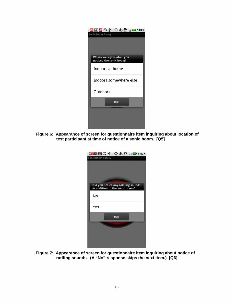
Figure 6: Appearance of screen for questionnaire item inquiring about location oftest participant at time of notice of a sonic boom. [Q5]

Figure 7: Appearance of screen for questionnaire item inquiring about notice ofrattling sounds. (A “No” response skips the next item.) [Q6]

17

Figure 8: Appearance of screen for questionnaire item inquiring about annoyance ofrattling sounds. (A “No” response skips the next item.) [Q7]

Figure 9: Appearance of screen for questionnaire item inquiring about degree ofannoyance of rattling sounds. [Q8]

18

Figure 10: Appearance of screen thanking test participants for reporting a sonicboom.

End-of-day interviews

The smartphone administered a second form of interview at a time of the test participant’schoosing at the end of the day. Whereas the test participant-initiated interview soughtinformation about short-term reactions to individual sonic booms, the end-of-day interviewfocused on reactions to an entire day’s worth of sonic boom exposures.6 The smartphonedisplayed questionnaire items in the same format as those illustrated in Figure 1 through Figure10 for the following questions:

How many sonic booms do you remember noticing today?

[If any booms are recalled] Considering all of the sonic booms that you noticed today, howannoyed would you say you were by all of them taken together?

[If more than one boom was recalled] Was any one particular sonic boom that you noticedtoday much more annoying than any of the others?

About what time of day did you notice the boom that was much more annoying than the restof the booms?

6 Test participants heard multiple sonic booms on some days, due both to supersonic military flight operations in thevicinity of Edwards AFB, and/or to multiple NASA flight operations specifically intended to produce low-amplitudesonic booms in the base housing area in the first half of November, 2011.

19

2.3 Distribution of smartphones to test participants

Half a dozen meetings were held between August and October of 2011 in an easily-accessible conference room at NASA Dryden Research Center to distribute smartphones andinstruct volunteer test participants in their use. (NASA had made separate contractualarrangements for recruiting test participants, including approval of recruiting methods by anInstitutional Review Board.) Appendix A contains the written instructions given to the testparticipants in the use of the smartphones.

Each test participant was provided with a smartphone and paraphernalia (holster, AC and carchargers, the manufacturer’s manual, a short written summary of the major features of thephones and of their tasks as test participants, etc.) to use as they would their own mobiletelephone for the duration of the study. They were requested to keep the phone with themthroughout their daily routines, both while at home and while away from home. If they desired,they were permitted to transfer contact files, pictures, and a pre-existing mobile telephonenumber to the smartphone so that it could serve as their primary mobile communication devicefor the duration of the pilot test. If they chose not to do so, they were permitted to continue touse another personal cell phone in addition to the supplied smartphones.

20

3 PRIMARY FINDINGS

A total of 5390 potential opportunities (49 test participants multiplied by 110 booms) forreporting notice of sonic booms occurred during the two week intentional booming period (from04 to 18 November 2011).7 For a variety of reasons, about two-thirds of these potentialopportunities proved not to be actual opportunities to assess residential reactions to sonic booms.In some cases, low-amplitude sonic booms may simply have been inaudible or otherwise escapednotice by test participants going about their daily business. Other reasons for not reportingbooms ranged from test participants’ lack of recognition of very low-amplitude booms as sonicbooms, to temporary absences of test participants from Edwards AFB, to uncharged smartphonesor smartphones otherwise without network access, and to a post hoc inability to unambiguouslylink boom reports with specific booms.8

Test participants used their smartphones to report notice of individual booms on 2152occasions. Of these 2152 reports, 1717 (79.8%) were made when participants were at home. Inthe remaining 435 cases, test participants filed reports while somewhere other than home.

Of the 1717 at-home reports, 1631 occurred when the respondent was indoors. Theremaining 86 outdoor responses were too few to merit separate analysis. In 1413 of the 1631cases (86.6%), test participants were indoors with active smartphones9, and their responses couldbe unambiguously linked to a specific dose sound level. These reports were received from asearly as 7:31 AM to as late as 4:24 PM.

The great majority (1333 of 1413, or 94.3%) of the boom reports concerned boomsintentionally created by NASA. The remainder (80 of 1413, or 5.7%) of the boom reportsconcerned adventitiously occurring sonic booms associated with other flight operations. Thelatter booms were generally of higher level than those intentionally created by NASA as low-amplitude booms. Test participants had no detailed prior information about the numbers,amplitudes, or sources of sonic booms.

3.1 Estimation of sonic boom exposure levels

In the two-week period of intentional booming during early November of 2011, testparticipants were exposed to a total of 110 sonic booms. Of these, 89 were intentionally created,and/or relatively low-amplitude sonic booms created by NASA aircraft, while 21 were generallyhigher amplitude booms created by military supersonic operations.

Measurements of sound pressure levels of intentionally created sonic booms within the basehousing area at Edwards AFB were made under separate contract. These measurements were

7 Many other opportunities for reporting sonic booms arose between August, 2011 and the start of the intentionalbooming period, but no consistent sound level estimates were available for most of booms reported prior to the startof the intentional booming period in November.

8 The principal reason that a report could not be unambiguously linked to an individual boom was that it wasreceived after the occurrence of a subsequent sonic boom. In one extreme case (a series of early morning booms, inrapid succession), few respondents provided interviews until the last boom of the series had occurred.

9 The smartphones provided status reports four times per hour to a central server, which confirmed them as “active”for purposes of this study: that is, operating, with adequate battery power and digital network access.

21

made at thirteen monitoring points located within a few hundred meters of test participants’homes. Exposure estimates were provided to Fidell Associates in the form of estimates of soundlevels for each of the booms immediately outside and inside the test participants’ homes.

Three different estimating methods were employed to assign doses to each respondent for theindividual booms. They were derived from geographically-interpolated measurements made atthirteen contractor-operated monitoring sites, and in some cases, at an additional, NASA-operated central monitoring site.

Method 1

The geo-referenced interpolation procedure involved complex, fine scale calculations thatattempted to take account of short-range meteorological influences on propagation of sonicbooms across the thirteen-station monitoring array. Figure 11 is a three dimensional exposuresurface produced in this manner for a single sonic boom. The figure illustrates pronounceddifferences in estimated sonic boom levels over short ranges for a single boom.

Figure 11: Exposure surface for a single sonic boom, calculated by short range geo-interpolation of sound level measurements made at thirteen monitoringpoints.

Point estimates of this sort may be useful for research purposes, such as constructingpsychometric functions for single event annoyance judgments for different noise metrics.However, they require many assumptions and engineering judgments which are difficult todocument, and may introduce statistical noise into dosage-response analyses.

22

Methods 2 and 3

Two other, less complex and less assumption-dependent sets of estimated sonic boomexposure levels were also constructed. One was a simple average of the measurements made atthe thirteen monitoring points. Simple averaging yielded sound levels representative of theaverage exposure of the entire base housing area to sonic booms, rather than single-eventexposure estimates at any test participant’s home. A third estimate of exposure levels was madefrom sonic boom levels recorded at a single monitoring point near the centroid of the basehousing area.

The latter two exposure estimates are similar to those which FAA relies upon for evaluatingaircraft noise impacts, and are thus more appropriate than point estimates at individual homes forconstructing dosage-response relationships between exposure to sonic booms and the prevalenceof high annoyance. For purposes of making policy decisions about the acceptability of exposureto sonic booms to residential populations, the most reasonable level of analysis is not theexposure of any particular individual to any specific sonic boom, but rather the prevalence of aconsequential degree of annoyance associated with area-wide exposure.

3.2 Distributions of levels of individual sonic booms noticed by test participants

For the 1413 reports of notice of sonic booms which could be unambiguously linked to aspecific sonic boom, the mean C-weighted SEL of the booms was 93 dB, with a standarddeviation of 6.2 dB. The corresponding A-weighted SEL values were 69 dB for the mean, and 9dB for the standard deviation. The mean of the maximum unweighted overpressures of thereported booms was 0.56 psf, with a standard deviation of 0.41 psf. The observed relationshipbetween maximum overpressure and CSEL is shown in Figure 39 on page 64.

3.3 Relationship among metrics of estimated sonic boom exposure levels

Estimates of sonic boom levels at the homes of test participants were based for the most parton contractor measurements at thirteen locations within the Edwards Air Force Base housingarea, and on noise modeling and contouring algorithms intended to interpolate the measurementsmade at the fixed locations to the homes of test participants. (Estimates were also based in somecases on additional sonic boom measurements made by NASA at a central location within thebase housing area.)

The estimates of sound levels and peak overpressures for each boom were expressed in unitsof a dozen noise metrics (including A-, C-, and Z-weighted sound exposure levels, variant formsof perceived and loudness levels, and sones and phons, for both outdoor and indoor cases), ateach test participant’s home address. A correlation matrix was prepared for the entire set ofestimated boom levels at test participants’ homes.

All of the estimated boom levels proved to be very highly correlated (typically, 0.90 orhigher) with one another.10 Thus, the various metrics differed from one another by little morethan scale factors and constants within the current set of field measurements, and were thereforenearly perfectly predictable from one another. This high degree of co-linearity among noise

10 This is not a novel finding. Mestre et al. (2011), for example, have recently demonstrated that most measures ofaircraft noise, including those calculated by FAA’s Integrated Noise Model software, are very highly correlated withone another.

23

metrics implies that for practical purposes of predicting the prevalence of high annoyance withsonic booms, any of the metrics is as good (or as poor) a predictor as any other.

Since much prior research on the annoyance of impulsive sounds related community opinionsto C-weighted noise measures such as CSEL and CDNL, these metrics were used for the currentdosage-response analyses as well. The grand average of single event CSEL values measured atthirteen monitoring stations for the booms occurring during the intentional booming period wasapproximately 92 dB, with a standard deviation of 8.1 dB and range of 34 dB across booms. Theaverage, standard deviation and range were 54, 8.3 and 27 dB, respectively, for the end-of-dayCDNL values.

3.4 Interpretability of findings of end-of-day interview data 95.3

Figure 12 is one illustration of the ready interpretability of responses to end-of-dayquestionnaire items. The figure plots percentages of respondents describing themselves asannoyed in varying degrees by each day’s exposure to sonic booms during the intentionalbooming period. The prevalence of reported annoyance tends to increase with CDNL, andsegregates itself into obvious groupings by degree of annoyance.

Figure 12: Illustration of interpretability of end-of-day annoyance judgments.

A similar example of the interpretability of responses to the immediate response interviews isshown in Figure 13. The noticeability and annoyance in varying degrees once again cluster indistinct groupings. Figure 13 displays percentages of at-home participants as a function of thesonic boom’s maximum overpressure, on a logarithmic scale. As in Figure 12, the percentages

24

increase with increasing sound dose. Furthermore, the groupings for the various types ofresponses are ordered in the expected high-to-low order. That is, the greatest percentages of testparticipants reported noticing sonic booms, while lower percentages of test participants describedthemselves as annoyed by them in greater degrees.

Figure 13: Illustration of interpretability of reports of notice and annoyance inimmediate (single event) interviews.

3.5 Demonstration of analyzability of immediate response interview data

Another goal of the current pilot test was to demonstrate that interview data collected bysmartphone could be statistically analyzed and otherwise treated in the same manner as interviewdata collected by other social survey methods. This was shown by performing a binary logisticregression through SPSS Binary Logistic. This analysis attempted to predict the probability ofrespondents describing themselves as highly (“very” or “extremely”, N = 76) annoyed on thebasis of five study variables: boom level (expressed in units of CSEL), day of study (1-9),ordinal number of boom for the day (1-27), time of day (AM or PM), and location of respondentat the time of occurrence of a boom (home indoors or home outdoors). Data were complete for1413 cases.

All of the variables except location at the time of occurrence of a boom were significantlyrelated to self-reports of high annoyance in univariate analysis. Prediction of high annoyancewas enhanced by entry of the five predictors into the equation (χ2

(5, N = 1413) = 95.30, p < 0.001).

25

The classification equation, although highly accurate, was unhelpful. The accuracy ofclassification was 95%, but was predetermined by the a priori odds of self reports of highannoyance. The classification equation merely assigned all of the cases to the “not highlyannoyed” category.

Because all of the predictors entered the equation simultaneously, each was adjusted foroverlapping variance with other variables. The only variable with sufficiently unique predictivevalue was CSEL (Wald = 66.14, p < .000). Two other variables that were marginally related tohigh annoyance were day-of-study (Wald = 3.43, p = .06) and ordinal position of boom in theday (Wald = 2.71, p = .10). Time of day and location of respondent did not contribute to theequation.

The final prediction equation was:

% Highly_annoyed = -20.04 + 0.167(CSEL) + 0.13(day-of-study) + 0.05 (ordinal_boom) -0.04(AM_PM) - 0.02 (location-of-respondent) [Eq. 1]

where:

CSEL = C-weighted sound exposure levelday-of-study = elapsed number of calendar days into study, with 04 Nov 2011 as day

number 1.ordinal_boom = the Nth sonic boom of the dayAM/PM = morning vs. afternoon distinction (AM=1, PM=2)location-of-respondent (indoors = 1, outdoors = 2)

No substantive use should be made of this equation other than as an indication that interviewdata collected by smartphone lend themselves to the same sorts of analyses that can be conductedon interview data collected by other means.

Appendix B contains additional descriptive analyses and summary graphics of the interviewdata. Since the sample of interview respondents was small and non-representative, the analysesof Appendix B are of interest primarily as examples of the sorts of fine-grained analyses thatsmartphone-based interviewing can support.

3.6 Development of formal dosage-response relationships

Relationships between judged annoyance and estimated exposure of test participants to sonicbooms were developed for opinions expressed in both immediate response (single-event) andend-of-day (cumulative exposure) interviews. The analyses reported here are limited to the twoweek intentional booming period in early November of 2011.11

11 A larger set of boom reports could also, in principle, be subjected to dosage-response analyses. These includereports made by test participants who were not at home, and reports of notice of sonic booms received prior to theNovember start of operation of the thirteen noise monitoring stations as early as August of 2011. Not all of the 49test participants were in possession of smartphones for all of this time period, and the amplitudes of only some of thesonic booms reported prior to November could be estimated with useful precision. Given that the primary goals ofthis pilot study were methodological rather than substantive, these analyses were not undertaken.

26

Annoyance judgments from the single event and cumulative exposure interviews wereanalyzed differently. The analysis of the single event interviews focused on the predictability ofreports of “high” (that is, “very” or “extremely”) annoyance among at-home test participantsfrom estimates of C-weighted sound exposure levels of each boom. The analysis of the end-of-day judgments of cumulative annoyance focused on comparing the prevalence of annoyance withcumulative exposure with prior findings using all end-of-day reports regardless of participant at-home status during the day.

In the single event case, percentages of test participants describing themselves as highlyannoyed by each boom were plotted against the CSEL of each boom. The numerator of thepercentage calculation included all of the highly annoyed test participants who reported noticinga sonic boom while at home (and for whom the sonic boom which they reported could bepositively identified).

The denominator for each percentage calculation took into consideration the numbers ofreports of notice of sonic booms received by the server, as well as the numbers of smartphones athome and answering the server’s periodic roll call (i.e., charged, turned on, and connected to adigital network) at the time of each boom. This calculation excluded from analysis all data fromtest participants who were 1) not at home at the time of occurrence of sonic booms, 2) those whomay have been at home, but whose cell phones could not be confirmed by server-based softwareas available for use shortly before the time of occurrence of sonic booms12, and 3) those whofailed to report notice of individual sonic booms prior to the occurrence of a subsequent boom.13

If it is assumed that test participants who failed to report notice of individual sonic boomssimply didn’t notice them, then it might be argued that excluding their data might lead to a slightoverstatement of the percentages of test participants highly annoyed by individual sonic booms.It is unlikely on its face, however, that test participants would have systematically failed tonotice highly annoying sonic booms.

A linear regression of percentages of highly annoyed test participants on CSEL values ofindividual booms at levels greater than 97 dB accounted for 51% of the variance in theassociation between individual boom levels and the prevalence of high annoyance (r = 0.72).14

Figure 14 shows that the growth of the prevalence of annoyance with level in the non-asymptoticregion was roughly 1.4 percent per one decibel increase in CSEL.

12 In a few cases, the smartphone status report immediately prior to a boom indicated the smartphone was probablyon its charger at the time of the boom. The fact that the participant provided a well timed match to a boomsuggested that the participant removed the phone from the charger to report the boom. In all such cases, thesmartphone remained off the charger until the next recharge was required.

13 Test participants sometimes completed multiple interviews shortly after reporting a particular boom. The firstinterview in such sets usually corresponded to the most recently heard boom. The remaining interviews were clearlyintended to respond to earlier booms which the participant had not previously reported. The order in which themissing interviews were provided could often be deduced by the answers to the questionnaire’s “how long ago”question (see Figure 2).

14 Note that this regression focuses on responses to only 18% (16 of 88) of the intentionally produced booms. Theother 82% of the booms were presented at levels in the asymptotic region which few test participants found to behighly annoying.

27

The percentage of at-home respondents describing themselves as highly annoyed is plottedagainst the arithmetic average values of CSELs derived by two estimation methods. The circlesrepresent CSEL values estimated at the residences of at-home participants, while the trianglesrepresent area-wide estimates of CSEL values at all of the boom monitors. This yields a pair ofplotting symbols for each sonic boom at the same points on the ordinate, but slightly differentpoints on the abscissa. The linear regression was computed from the triangular data points (i.e.,using the area-wide average CSEL estimate). In general, the two estimates of sound levels ofbooms are within ± 0.5 dB of one another.

Figure 14: Linear regression of percentage of at-home respondents highly annoyedby C-weighted sound exposure levels estimated by two methods.

Responses to interviews about the cumulative annoyance of an entire day’s exposure to sonicbooms were analyzed differently (cf. Section 5.3), so that they could be compared directly withprior findings summarized in a report of the National Research Council’s Committee on Hearing,Bioacoustics and Biomechanics (Fidell, 1996).

28

4 DISCUSSION OF METHODOLOGICAL FINDINGS

The findings presented in the prior section show that community reaction to sonic boomexposure may be usefully assessed using smartphone-based interviewing methods. Testparticipants complied well with instructions for reporting notice of sonic booms, whether indoorsat home or outdoors and away from home. They repeatedly and reliably completed briefinterviews about their short and long term reactions and opinions concerning exposure to booms.The responses to interviews seeking both short- and long-term opinions about sonic booms weresystematically interpretable, and comparable to those produced by conventional social surveyinterviewing methods. This section contains further discussion and additional details about someof these findings.

4.1 Reports of notice of individual sonic booms (immediate responses)

The 49 test participants provided 2152 reports of notice of individual sonic booms during theintentional booming period.15 Table 2 shows the locations of test participants at the times thatthey reported sonic booms. The bulk of them (86.4%, or 1860/2152) were indoors either athome or elsewhere when they reported noticing booms. Of these, 1631 (87.7%) were indoors athome at the time of the boom. Only 1413 (86.6%) of these 1631 responses, however, could beunambiguously linked to a sound level dose.

Table 2: Locations of test participants when they reported individual sonic booms

Locus of Respondent Indoors Outdoors Sum

At Home 1631 86 1717

Away From Home 229 206 435

Sum 1860 292 2152

4.2 Response latencies and interview durations

Respondents indicated that 86% of their immediate reports (1845/2152) of notice of sonicbooms during the intentional booming period were lodged within a few minutes of theiroccurrence. Figure 15 shows the log normal-appearing distribution of response latencies.Several reports with latencies in excess of 900 seconds (15 minutes) are omitted from the figure.The average number of observations in the omitted 10-seconds wide bins do not exceed 1. Themedian response time, however, was 41.9 seconds.16 Section 11.2 shows cumulative distributionfunctions and the varying percentages of respondents who responded after specific latencyperiods.

15 Not all of these reports could be unambiguously associated with individual sonic booms, particularly when longresponse latencies coincided with short inter-boom intervals.16 The distribution is so skewed that its arithmetic mean is not a useful indication of average response times.

29

Figure 15: Distribution of response latencies for reporting individual booms withinthe first fifteen minutes (900 seconds) of their occurrence.

Figure 16 displays the first 2 minutes (120 seconds) of the same log normal-appearingdistribution of interview durations, in five second wide bins. This plot provides greaterresolution for the initial portion of the distribution, and reveals that the mode of the distributionlies somewhere between 10 and 15 seconds.17

4.3 Opinions about cumulative exposure to sonic booms (end-of-day interviews)

Table 3 and Figure 17 show the numbers and completion rates of end-of-day interviews foreach day during the intentional booming period. The overall response rates compare favorablywith those achievable by conventional social survey (telephone) interviewing methods.

17 The response database includes information about the time (in milliseconds) which respondents required toanswer each question. Future detailed analyses, if desired, can be conducted of this information. If a boom werenoticed while an interview concerning reactions to a prior boom, for example, the point in an interview at which anadditional boom occurred could be readily determined.

30

Figure 16: Distribution of durations of immediate response interviews

Table 3: Numbers of test participants completing end-of-day interviews on each dayof intentional booming period

Date Number ofInterviews

ResponseRate

11/04/11 38 77.6%

11/07/11 33 67.3%

11/08/11 41 83.7%

11/09/11 39 79.6%

11/10/11 37 75.5%

11/14/11 38 77.6%

11/15/11 41 83.7%

11/16/11 43 87.8%

11/17/11 33 67.3%

11/18/11 34 69.4%

Total 377 76.9%

31

Figure 17: Percentages of test participants completing end-of-day interviews oneach day of the intentional booming period.

4.4 Debriefing interviews

About half of the test participants attended a meeting at Dryden Research Center organized tothank them for their participation in the pilot test, and to provide them with $50 gift certificates.They also completed informal, written debriefing interviews. The test participants uniformlyindicated that they had enjoyed participating in the pilot test, were satisfied with the level oftechnical support provided, would willingly participate again in any future extension of the testprogram, and would recommend participation to their friends. They expressed no dissatisfactionwith any aspect of the test protocol, and only minor dissatisfaction with the necessity forrecharging their smartphones every night.

4.5 Adequacy of recruitment incentives

The only direct incentive offered for participation in the pilot test was cost-free personal useof a smartphone for the duration of the study. The 49 participants were awarded $50 giftcertificates at the end of the study, after they had already indicated their willingness to take partin the study. The award was made solely in the interests of maintaining parity with participantsrecruited into a parallel NASA-sponsored study conducted at the same time.

Among spouses of active duty Air Force personnel residing in base housing, participation inthe study appears to have been sufficiently enjoyable that no inducement beyond free use of asmartphone was required. It is unclear whether the general population would be as willing toparticipate in a similar study conducted elsewhere.

32

5 DISCUSSION OF SUBSTANTIVE FINDINGS

5.1 Estimation of cumulative exposure to sonic booms

As noted earlier, a contractor measured sonic boom levels at thirteen spatially distributedsites within the base housing area during the intentional booming period. (NASA DrydenResearch Center operated a fourteenth monitor near the centroid of the base housing area aswell.) Three estimates of cumulative daily exposure of test participants to sonic booms duringthe intentional booming period were developed from these measurements.

First, estimates of daily exposure were developed from predictions of individual boom CSELvalues at each test participant’s home. This required numerous assumptions and considerableprocessing of the measurements to create and contour an expected exposure surface, as describedin Section 3.1 and illustrated in Figure 11. Second, estimates of daily exposure were developedfrom the means of the measured levels for each of the booms at each monitoring site. Third,estimates of daily exposure were developed from a single, centrally located monitoring site nearNASA Dryden’s central monitoring position.

Table 4 compares the estimates of CDNL18 values derived by the above three methods. Themean differences across days among the three estimates are meaninglessly small (less than 0.2dB) in the context of the uncertainty (±0.5 dB) of the original measurements. Further, thecorrelations among the various estimates of daily cumulative exposure are all in excess of r =0.99. It follows that in these circumstances, the more complex measurement and estimationmethods yield little or no benefit.

18 Because no sonic booms occurred during the DNL “nighttime” period, these figures do not differ from 10 or 12hour C weighted Leq values.

33

Table 4: Comparison of variously estimated CDNL values and percentages ofannoyance reports in varying degrees

TestDay

Date

CDNL Noise Exposure Estimates (dB) Observed Annoyance

GrandMean of 13Monitors[1]

Mean ofIndividualHouseholdEstimates

SingleMonitor atInterview

AreaCentroid

Slightly+Annoyed

Moderately+ Annoyed

HighlyAnnoyed

1 11/04/11 54.7 54.6 54.2 47.4% 7.9% 0.0%

2 11/07/11 55.6 55.5 55.6 33.3% 12.1% 3.0%

3 11/08/11 55.8 55.8 55.8 31.7% 17.1% 4.9%

4 11/09/11 56.8 56.8 56.4 43.6% 10.3% 2.6%

5 11/10/11 47.5 47.3 47.4 21.62% 2.7% 0.0%

6 11/14/11 59.7 59.6 59.8 57.9 23.7 5.3%

7 11/15/11 60.6 61.0 60.5 68.3 31.7% 12.2%

8 11/16/11 67.4 67.4 67.5 88.4 51.2% 23.3%

9 11/17/11 43.6 43.5 43.3 24.2% 6.1% 3.0%

10 11/18/11 40.7 40.4 40.4 14.7% 2.9% 2.9%

Coefficient ofDetermination [2] - - - - 0.999 0.999

Mean Difference - - - - -0.02 -0.18

Std Dev of Differences - - - - 0.17 0.20

[1] Predictor variable for computing correlations between remaining two CDNL estimates.[2] Variance accounted for (r2).

The data of Table 4 are plotted in Figure 18 to illustrate the practical implications of the highcorrelations among estimated exposure levels. The curve fitted to the data figure is a minimalrms error fit of the data to an effective loudness function (described in greater detail in the nextsection of this report), using the “grand mean of 13 monitors” data as the CDNL predictorvariable.

34

0%

10%

20%

30%

40%

50%

60%

70%

80%

90%

100%

35 40 45 50 55 60 65 70 75

Estimated CDNL (dB)

Pe

rce

nt

Hig

hly

An

no

yed

Mean of Individual Household Estimates

Mean of 13 Monitors

Single Centroid Monitor

CTL Curve Fit to 13 Monitor Means

Figure 18: Comparison of relationship between high annoyance and mean CDNLvalues for each day of intentional booming period as estimated by threemethods.

5.2 Dosage-response analyses of current findings

Fidell et al. (2011) and Schomer et al. (2012) have recently published descriptions of asystematic, first-principles approach to inferring dosage-response relationships betweencumulative transportation noise exposure and the prevalence of high annoyance in communities.The approach is based on the assumption that the rate of growth of annoyance in a communityclosely resembles the rate of growth of the effective (that is, duration-corrected) loudness ofnoise exposure. The slope of the dosage-response relationship is therefore fixed, while a secondvariable, a Community Tolerance Level, or CTL, is used to characterize the position of thedosage-response relationship on the exposure axis.

Annoyance prevalence rates in CTL analyses are predicted as

p(HA) = e-(A/m), [Eq. 2]

where:

A is a scalar, non-acoustic decision criterion originally described by Fidell et al., (1988),and

m is an estimated noise dose, calculated as

m = (10(DNL/10))0.3 [Eq. 3]

35

The value of the scalar quantity A in a given community is that which minimizes the root-mean-square error between predicted (cf. Eq. 2) and empirically measured annoyance prevalencerates (Green and Fidell, 1991; Fidell et al., 2011). Since m is just a transform of DNL, aquantitative estimate of the tolerance parameter, A, can be derived from knowledge of %HA andDNL at an interviewing site. When the annoyance prevalence rate (p[HA] ) is held constant, thedecision criterion, A, and the transformed noise dose, m, are linearly related by19:

A = m · ln[1 / p(HA) ] [Eq. 4]

Figure 19 shows the fit of the annoyance prevalence rates measured in the current pilot studyto the predicted dosage-response relationship. Note that cumulative exposure is expressed in A-weighted units in Figure 19. The product-moment correlation between predicted and observedannoyance prevalence rates is a nearly perfect r = 0.94 (R2 = 0.89).20

0

10

20

30

40

50

60

70

80

90

100

15 20 25 30 35 40 45 50 55

Day-Night Average Sound Level (dB)

Pe

rce

nt

Hig

hly

An

no

ye

d

CTL: 60.90 dB

RMS Error: 0.084

r squared: 0.892

Figure 19: Fit of the current data to the annoyance prevalence rates predicted byCTL analysis.

A CTL value is defined as a value of (in this case) CDNL at which half of a communitydescribes itself as “highly” annoyed by exposure to sonic booms. The CTL approach can also beextended to create dosage-response relationships for degrees of annoyance less extreme than“highly annoyed.”

19 Equation 4 simply rearranges the terms of Equation 2.20 The product-moment correlation for C-weighted DNL values is trivially higher (r = 0.95),

36

Figure 20 compares dosage-response relationships for the prevalence of annoyance in threecumulative21 categories. “Annoyed to any degree” is the sum of responses “slightly”,“moderately,” “very,” or “extremely”; “moderately or more greatly annoyed” is the sum ofresponses in the “moderately,” “very,” and “extremely categories; and “highly annoyed” is thesum of responses in the “very” and “extremely” categories. (Note that a yellow diamond plottingsymbol for moderate or greater annoyance at 41 dB lies immediately behind an orange circlesymbol for high annoyance at the same CDNL value.)

0%

10%

20%

30%

40%

50%

60%

70%

80%

90%

100%

35 40 45 50 55 60 65 70 75 80

Mean CDNL of Sonic Boom Exposure from 13 Monitors for Each Day ofIntentional Boom Period (dB)

Pe

rce

nt

An

no

yed

Annoyed in any degree

Moderately or more greatly annoyed

Highly Annoyed

CTL fit to annoyed in any degree

CTL fit to moderately or more greatly annoyed

CTL fit to highly annoyed

12.6 dB 8.5 dB

Figure 20: CTL-based relationships between variously defined degrees of annoyanceand estimated CDNL values

The decibel differences shown at the median of the curves are an indication of thedifferences in sound levels associated with the definitions of annoyance in varying degrees. TheCDNL values of the data points in Figure 20 are computed using the area-wide averagingmethod at all thirteen noise monitor sites.

21 In principle, the same analysis could be applied to annoyance in individual (non-cumulative) annoyancecategories. Analyses of this sort could permit more detailed regulatory analyses of sonic boom exposure levelswhich could identify, for example, exposures which are only slightly annoying. In practice, the current data set doesnot contain enough information to be informative about reactions to sonic booms at higher exposure levels.

37

5.3 Comparisons of dosage-response relationship for end-of-day interview reports ofannoyance with prior findings

For reasons noted earlier, the substantive findings of the current pilot test about therelationship of annoyance to sonic boom exposure should not be viewed as definitive. It isnonetheless of interest to compare them with prior findings about the relationship betweencumulative exposure to sonic booms and the percentage of people reporting high annoyance dueto sonic booms.22

Figure 21 shows that the current findings about the relationship between exposure to sonicbooms and the prevalence of a consequential degree of annoyance with them, shown as filled redplotting symbols, are quite similar to observations made in Oklahoma City almost half a centuryago (Borsky, 1965), shown as open blue plotting symbols.23

Figure 22 compares the current findings (filled red plotting symbols) with all of the data inthe 1996 CHABA report (Fidell, 1996) on the annoyance of high energy impulsive sounds. Theadditional data include the findings of interviews about annoyance from sources such as artilleryand shooting range noise, as well as the findings of a social survey on the annoyance of sonicbooms conducted in small communities near the U.S. Air Force’s Nellis Range in easternNevada and Edwards Air Force Base (Fields et al., 1994).

The value of CTL for the pilot test data set is 61 dB. This implies that half of the currentsample would describe itself as highly annoyed by boom exposure at a DNL value of 61 dB. Asillustrated in Figure 23, this value of CTL is notably lower than the grand mean for all aircraftsurvey findings, or Lct = 73.3 dB (per Fidell et al., 2011). The open blue plotting symbols inFigure 23 represent the findings of 44 studies of the annoyance of conventional (sub-sonic)aircraft noise. The filled red plotting symbols in Figure 23 are the findings of the present pilottest. (Note that three plotting symbols of DNL less than 30 dB and high annoyance values of 3percent or less are not shown in this figure.) In other words, A-weighted decibel for decibel, testparticipants were 12 dB less tolerant of sonic booms than of subsonic aircraft noise.

The abscissa of Figure 23 plots A-weighted DNL (not CDNL), because aircraft noiseexposure is conventionally measured in units of DNL. Assuming that the findings of the currentpilot test are generalizable to a wider population, Figure 23 indicates that exposure to sonicbooms (red data points) of low level tends to highly annoy greater percentages of communityresidents than does subsonic aircraft noise of similar exposure level.

22 Although smartphone-based interviewing methods permit adjustments to be made to individual CDNL estimates(for times when respondents are away from home), no effort was made to do so in the current analysis. Prioranalyses of dosage-response relationships aircraft noise exposure all summarize geographic associations betweencommunity-wide outdoor sound levels and the prevalence of annoyance. Since reports of annoyance with sonicbooms made while respondents were away from were excluded from the current analysis, changing the predictorvariable from community-wide to personal exposure probably would have had little effect on the findings in anyevent.

23 Note that these comparisons are made in C-weighted units to facilitate comparisons with prior findings of socialsurveys of reactions to sonic booms.

38

0

5

10

15

20

25

30

35

40

35 40 45 50 55 60 65 70

CDNL (dB)

Pe

rce

nt

Hig

hly

An

no

ye

d

Oklahoma City

Current Findings

Figure 21: Similarity of current findings (filled red plotting symbols) to a priordetermination (Borsky, 1965) of the prevalence of high annoyance withsonic booms.

0

5

10

15

20

25

30

35

40

35 40 45 50 55 60 65 70

CDNL (dB)

Pe

rce

nt

Hig

hly

An

no

ye

d

Prior Observations

Current Study

Figure 22: Comparison of current data (filled red plotting symbols) with priorobservations cataloged by Fidell (1996).

39

Figure 23: Prevalence of annoyance with low-amplitude sonic booms (filled redplotting symbols) in relation to similar findings of 44 other studies of theannoyance of aircraft noise (Fidell et al., 2011.)

40

6 LESSONS LEARNED

If the methods developed in the present pilot test are to be applied on a larger scale in afuture study, several modifications of the methods could reduce costs and improve the overallefficiency of data collection.

6.1 Recommendations about scheduling of intentional exposures to sonic booms

When paid laboratory subjects are asked to make judgments about the annoyance of testsounds, experimental convenience and cost are major determinants of the rate and number ofjudgments that they are asked to make. In a social survey-like field study intended to collectinformation from unpaid volunteers about the effects of sonic booms in residential settings, otherfactors must also be weighed in scheduling controlled exposures to sonic booms. In particular,the advantages in face validity, reliability, and accuracy of subjective assessment of sonic boomimpacts which smartphone-based interviewing offer should take priority over the experimenter’sconvenience in producing and scheduling sonic booms.

Convenient as smartphone-based interviewing may be, reporting notice of a boom stillrequires a minimal diversion of attention from daily routine. The ability and/or willingness oftest participants to promptly and consistently report notice of sonic booms depends on severalfactors: particularly, the inconvenience of the method of filing a report, the inter-boom interval,and possibly the number of booms occurring within short periods of time.24

Smartphone-based interviews of the sort described in this report are very convenient. Theyare initiated with trivial effort, require little time to complete, and provide test participants withsome control over the timing of the unavoidable short interruption of their ongoing activities.Pressing a button on a device which is customarily ready-to-hand, and which respondentscommonly use for many other purposes, requires considerably less time and bother than otherforms of interviewing.

The other factors noted above that affect the ability and willingness of people to repeatedlyreport notice of sonic booms – the inter-boom interval, the number of booms occurring withinshort periods of time, and the time of occurrence of booms – are under the experimenter’scontrol. The pace and timing of controlled exposure to sonic booms should not exceed the paceof exposure in settings to which inferences about sonic boom impacts are to be generalized.Further, the rate and number of sonic boom exposures should not be so great as to imposeunreasonably on the good will of volunteer study participants, nor on their ability to respondpromptly and reliably.

The pace of exposure should also not be so great as to complicate the association ofresponses with exposure episodes. If two or more sonic booms occur in rapid succession, it is

24 Incentives offered for prompt or accurate responding could conceivably improve the promptness and reliability ofreports of sonic booms. In principle, for example, small incentives could be offered for interviews completed withina minute or two of occurrence of a sonic boom, or for total numbers of hits (reports received within a few minutes ofthe occurrence of sonic booms) per day. Small disincentives could likewise be imposed for false alarms (reports ofnon-existent booms). These measures were not taken in the present study in order to preserve as muchcomparability as possible with the conditions of prior field surveys about the annoyance of sonic booms. Suchmeasures could be worth considering in similar future studies, however, depending on detailed research goals.

41

sometimes not possible to unambiguously attribute responses to specific noise events. Thus, in aseries of successive booms within a brief period of time, delayed reports of notice of earlier sonicbooms may not be distinguishable from prompt responses to later booms, leading to collection ofunanalyzable data.

This situation arose on several occasions in the present study, most notably on a day whenmultiple intentional and adventitious booms occurred within minutes (or even seconds, in somecases) of one another. Closer coordination of shared supersonic airspace to avoid temporal“collisions” of sonic booms within a target residential area can be both costly and inconvenient.However, planning of intentional exposure schedules should not give greater weight to the costsof producing individual sonic booms than to unambiguous attribution of responses to them.

If a minimal inter-boom interval of at least a quarter hour cannot be maintained for otherreasons, then test participants should be given explicit instructions about the order in which toreport their prompt and delayed reactions to sonic booms. These instructions should indicate thattest participants must always respond first to the most recent boom noticed. In the event thatthey recall one or more prior unreported same-day booms after reporting notice of the mostrecent one, they should be instructed to file delayed reports for each in a specific order,preferably the most recent prior unreported boom first. Alternatively, they could be instructednot to report sonic booms if more than five minutes have elapsed since the time of notice.

It may also be helpful to seek greater temporal resolution in responses to the question, “Howlong ago did you notice a sonic boom?”, than “within the last few minutes”, “within the last halfhour”, and “more than a half hour ago.” Greater temporal precision may be unnecessary in manycases, but it may be helpful in others. For example, suppose hypothetically that a test participantknown to have been at home has failed to report three booms in succession. The failure to reportthree booms could simply be due to their low amplitude, but the booms could also have beennoticed at times when it was inconvenient for the test participant to file a prompt response.

When the hypothetical test participant finally reports noticing a later boom, and then recallsnoticing (but not reporting) two prior booms that day, to which of these three booms should thetwo delayed reports be attributed? This situation occurred in the current study, when two testparticipants were exposed to four booms in one morning. They both provided their first responseof the morning shortly after the fourth boom, and both indicated that they had noticed the boom“within the last few minutes.” It was therefore possible to unambiguously attribute theirresponses to the most recently occurring boom.

Next, however, both test participants filed delayed reports of noticing a single additionalboom, when in fact three had been produced. Both test participants also indicated that thepreviously unreported boom had been noticed more than half an hour ago. The only boom thatcame close to occurring in this time period was the first of the morning, so their reports of theirdelayed responses were assigned to that boom25.

25 Attribution of delayed responses to prior booms could also take into consideration boom amplitudes, but somemight object that assuming that responses were attributable to higher level booms forces a positive slope on anyresulting dosage-response relationship. The region of the dosage-response curve of greatest interest – where itsslope differs from its lower asymptotic value – is the one in which conclusions are most sensitive to such dataprocessing assumptions.

42

In another case, the study design exposed test respondents to five booms between 7:20 and8:03 AM. Most of the responses to this series of booms were not received until after the last ofthem, suggesting that test participants either were not yet fully awake when the booms began, orthat they may not have had their cell phones handy shortly after awakening.

On yet other occasions when test participants belatedly reported noticing more than onepreviously unreported boom later in the day, they had already provided an unambiguous reportof reactions to the next most recent boom. To avoid errors of attribution of responses to boomsin such cases, it was sometimes necessary to simply entirely exclude observations from analysis.Although discarding data in such cases may be preferable to erroneous attributions of reports ofboom effects to particular booms, it is nonetheless wasteful to do so if the problem can beavoided by broader consideration of all of the constraints on the design of the exposure schedule.

6.2 Recommendation for extension of scale of application of technique

If samples of hundreds or thousands of respondents are anticipated in a future study, it maynot be cost-effective to provide each respondent with a government-furnished smartphone andservice contract. An obvious solution to minimizing such costs is to permit respondents todownload the “Report Boom” application to their own personal Android smartphones and/orother internet-enabled mobile devices, possibly including tablets.26 Some of the implications ofdoing so are noted in Section 6.4.

1) The interviewing application code should be checked to confirm that it works as intendedon Android platforms later than the Droid2. The application code may not need to be polledseveral times an hour to determine the host phone’s location, but may need to be modified topermit remote deactivation.

2) Since study participants will not be using government-configured smartphones, it may benecessary to confirm that other applications will not interfere with the sonic boom reportingapplication.

3) Methods of recruiting study participants will have to be revised as suitable to residentialconditions of target communities, which may be less constrained than those of Edwards AFB.For example, depending on the duration of the intended study, alternative forms of incentives forparticipation may have to be devised. These could range from small, one-time payments fordownloading the application to daily payments for continued study participation. If consistentwith other study goals, payments might also be made for prompt reporting of bona fide sonicbooms, with adjustments for false alarms.

4) If it is suspected that the opinions of smartphone users about sonic booms differsystematically from those of other residents, measures may have to be taken to quantify andcorrect for such potential biases. It may also be necessary to devise methods for determining thetotal numbers of test participants actively participating in the study on any given day, or at thetime of occurrence of any particular boom, so that the denominator for calculations ofpercentages of respondents similarly affected by each boom can be confirmed.

26 It is also possible, of course, to port the Android software to iOS (Apple) smartphones, but it is unclear whatfurther constraints this might impose on the design or cost of near-real time interviewing software. Apple might ormight not insist on incorporating (or removing) certain design features, and the terms of Apple’s privacy policy andend user agreement might conflict with the need to protect personally identifiable information.

43

The personnel costs of measures of this sort may be unaffordable in larger scaleimplementations of smartphone interviewing studies, but are probably not essential either.Communication between test participants and project personnel should probably be limited totext messaging.

6.3 Porting of application code to iOS (Apple) devices

The “Report Boom” application was developed for smartphones which use the Androidplatform. Android and iOS (Apple) mobile devices currently have roughly equal shares of arapidly growing market. If the Report Boom application is to be made available for freedownloading within defined geographic areas or telephone exchanges, it could be helpful to portthe application to iOS platforms. There is little reason to believe that opinions of users ofdifferent brands of smartphones about sonic booms differ systematically, but in any local market,one brand or another of smartphone may be more popular, or provide more reliable networkconnectivity.

Porting the application could impose constraints on the design or cost of near-real timeinterviewing software. Most features of “Report Boom” application would transfer directly andsimply to other platforms, although smartphone location reporting would probably requiremodification. Moreover, because Apple exerts considerable proprietary control over iOSapplications, it might insist on incorporating (or removing) various design features, and the termsof its privacy policy might conflict with the need to protect personally identifiable information.

Some additional implications of porting Report Boom to other platforms to facilitate alarger-scale study using respondent-owned devices are noted below.

1) The sonic boom reporting application code must be checked to confirm that it works asintended on Android platforms other than the Droid2, as well as on iOS platforms (if they are tobe used).

2) Since study participants will not be using government-configured smartphones withknown configurations and options, it would be necessary to confirm that other applications onthe participants’ smartphones will not interfere with the sonic boom reporting application.

3) The pilot study made extensive personal support available to test participants. Testparticipants were provided with a toll-free telephone number to call at any time of day fortechnical assistance, including questions about test procedures, reports of broken or misplacedequipment, and the like. The status of test participants’ smartphones was also closely monitored,and reminder calls were placed to test participants who had not used their smartphones forextended periods, were not at home for extended periods, or had forgotten to recharge theirphones. The personnel costs of measures of this sort may be unaffordable in larger scaleimplementations of smartphone interviewing studies, but are probably not essential either.Communication between test participants and project personnel could probably be accomplishedby text messaging, email and voicemail.

4) Before applying the sonic boom reporting software to an expanded participant population,several scalability and system design issues need to be addressed. The most notable questionsconcern whether a major increase in numbers of participants affects smartphone-to-servercommunication, and whether current database creation, downloading, and maintenanceprocedures are adequate to support a much larger study. If it is suspected that the opinions ofsmartphone users about sonic booms differ systematically from those of other people, measuresmay have to be taken to quantify and correct for such potential biases. It may also be necessary

44

to devise methods for determining the total numbers of test participants actively participating inthe study on any given day, or at the time of occurrence of any particular boom, so that thedenominator for calculations of percentages of respondents similarly affected by each boom canbe confirmed.

5) Methods of recruiting study participants will have to be revised as suitable to residentialconditions of target communities, which may be less constrained than those of Edwards AFB.For example, depending on the duration of the intended study, alternative forms of incentives forparticipation may have to be devised. These could range from small, one-time payments fordownloading the application to daily payments for continued study participation. If consistentwith other study goals, payments might also be made for prompt reporting of bona fide sonicbooms, with adjustments for false alarms. These measures were not taken in the present study inorder to preserve as much comparability as possible with the conditions of prior field surveysabout the annoyance of sonic booms. Such measures could be worth considering in similarfuture studies, however, depending on detailed research goals.

6.4 Improvements to participant instructions

The process of associating specific interview data with specific sonic booms was largelyautomated by means of spreadsheet macros. Nonetheless, manual intervention was sometimesrequired to resolve ambiguities when reports of notice of sonic booms lagged their occurrence bylengthy intervals (e.g., half an hour or more), and/or when additional booms occurred before testparticipants completed interviews about their reactions to one or more earlier booms. Most suchambiguities could be resolved through careful examination of individual cases. In some cases,however, it was necessary to discard otherwise-valid interview data when it was not possible todefinitively associate particular responses with particular booms.

Such cases were difficult to resolve because the order in which test participants reported theirreactions to multiple prior sonic booms was unclear. The response categories of QuestionnaireItem 1 (“How long ago did you notice a sonic boom?”) were “within the last few minutes”,“within the last half-hour”, and “more than a half-hour ago?” When multiple booms occurred inrelatively rapid succession, these categories were not always sufficient to permit confidentassignment of interview data to individual booms.

In principle, greater temporal resolution in response categories could help to clarifyassignment of late interviews to individual booms. For example, respondents might be asked toselect whether a boom was noticed within the last 10 minutes, 10 – 20 minutes ago, 20 – 30minutes ago, etc. At some point, however, test participants may not be able to recall whenbooms occurred with meaningful precision, and may find the requirement to keep track of whenbooms occurred to be frustrating and inconvenient.

Other solutions to this problem are conceivable as well. They include switching from a freeresponse paradigm to some other form of reporting (say, hourly, or prompted); instructingrespondents not to report notice of sonic booms if more than five minutes have elapsed betweenthe time of notice and the time of reporting; or providing specific instructions to test participantsabout the order in which reactions to previously unreported booms are provided. Yet anotherapproach would be to enforce a minimal inter-boom interval long enough to unambiguouslyassign 90% or 95% of the interviews to particular sonic booms.

45

6.5 Minor improvements to features of smartphone reporting application

Several minor improvements to the application software may also be useful:

1) The most common operational glitch in the pilot study was an occasional failure by someparticipants to keep their smartphones’ batteries charged. Participants in future studies couldreceive “low battery” reminders of various forms. These might include pop-up messages fromthe smartphone software, text messages to the smartphone and perhaps to other phones known tobe nearby, emails to the participants’ email accounts, “robo-call” voicemails to their landlines. Ifa smartphone’s battery charge level were so low that only one or two sonic boom reports couldbe successfully accomplished, the software could (for example) temporarily block othersmartphone operations.

2) Tradeoffs between battery life, frequency of automated communications betweensmartphones and the central server, and the level of detail of information reported to the server,should be re-examined. On the one hand, newer model smartphones may have enough power tolast for more than a day in the present application. On the other hand, it might be possible toidentify and report the smartphone’s location and status less frequently at some times of day thanat others (e.g., at night). It might also be possible to minimize the power required for GPS-baseddetermination of “at-home” status by relying more heavily on home local area wi-fi or 3/4Gwireless connectivity.

A change in study design should also be considered, such that status reports from individualsmartphones would be solicited only immediately prior to the scheduled time of occurrence ofknown sonic booms. This design modification might be appropriate for exposure situations inwhich the total numbers of booms audible to test participants could be carefully controlled (i.e.,in areas remote from supersonic flight corridors, military operating areas, joint military/civilairspace, etc.), and in which the frequency of exposure to booms could be limited to a few perday.

3) Every smartphone in the pilot test was equipped with a COTS27 application that provideddata security, limited unauthorized use of the device, defended against malicious applications,protected against viruses and other malware, and allowed the smartphone to be deactivatedremotely if it was lost or stolen. These features would not necessarily be required if participantsin a future study were using their own, rather than government-furnished devices. Participantscould be advised to install such protective code on their smartphones at their own expense. Thesonic boom application code should nonetheless be modified to permit remote deactivation.

4) Improvements might be useful in automated data quality control capabilities, to morequickly and thoroughly perform some of the operations that were done manually by theexperimenters during the pilot test to detect anomalous conditions (such as duplicate entries) inthe accumulating databases. If communication with field instrumentation were possible, thetimeliness of assignment of boom reports to specific booms could also be greatly improved,while minimizing manual post-processing.

6.6 Measures useful for estimating exposure levels over a wide area

If an expanded study entails exposing residents to sonic booms over areas greater than a fewsquare kilometers, costs for installing and servicing dense arrays of monitoring instruments couldwell prove prohibitive. In such cases, a coarser spatial sampling of boom levels suffices to yieldboom level estimates of adequate precision. As shown in Section 5.2, complex measurements of

27 Commercial Off-The-Shelf

46

sonic boom levels at multiple points, intended to yield estimates of sonic boom levels at thehomes of individual test participants, produce no useful increase in precision of estimation ofcommunity response to sonic boom exposure.

The goal of large scale measurement of boom levels should not be to validate or calibratemodel-predicted, point estimates of boom levels at the residences of study participants, but ratherto estimate wide-area exposure levels. For such purposes, a small number of boom monitoringpoints is more than adequate, since fine scale variation in boom levels over short ranges is not ofinterest in the context of combining opinions of residents of hundreds or thousands of householdsmany kilometers distant from one another.

47

7 CONCLUSIONS

Smartphone-based interviewing is a useful adjunct and a powerful addition to conventionalmethods of assessing the effects of sonic booms on exposed populations. Compliance withinstructions for smartphone use to report notice of sonic booms in the current pilot study wasexcellent. No test participants voluntarily failed to complete the study; the data were readilyinterpretable; and nearly all test participants indicated that they would choose to participate insuch a study again if given the opportunity, and would recommend participation in such a studyto friends.

The findings of the current study were also consistent with those of earlier social surveys ofthe annoyance of exposure to high energy impulsive sounds. The similarity of the presentfindings to those of Borsky (1965) is striking.

Several modifications of details of the pilot test procedures for smartphone-based assessmentof sonic boom impacts on residential population could facilitate their implementation on a largerscale. These include the following:

1) The application code for reporting booms could be generalized beyond a single operatingsystem, and to permit use with Internet-enabled portable communication devices (e.g., tablets)other than smartphones.

2) The method of estimating levels of exposure to sonic booms should be simplified toimprove characterization of uncertainty and estimation of dose levels.

3) Specific instructions should be provided to test participants about the order in which theyshould file delayed reports of notice of sonic booms.

4) Design of the schedule of intentional exposure to sonic booms should give greaterconsideration to maintaining a minimum inter-boom interval of at least fifteen minutes to avoidcollection of unanalyzable response information.

48

8 ACKNOWLEDGMENTS

The authors thank Larry Cliatt and Ed Haering of NASA Dryden Research Center forassistance with field arrangements for data collection. We are also grateful to Matthew Sneddonfor assistance in processing sonic boom measurements; to John Roses of Interviewing Service ofAmerica for quality control and related assistance during field data collection; to Linda Fidell forassistance with statistical analyses; and to Gregory Milette of Gradison Technology forassistance in software development.

49

9 REFERENCES

Borsky, P. (1965) “Community reactions to sonic booms in the Oklahoma City area”, USAFAerospace Medical Research Laboratory, Report AMRL-TR-65-37, Wright-Patterson Air ForceBase, OH.

Fidell, S. (ed.) (1996) “Community response to high energy impulsive sounds: anassessment of the field since 1981”, Working Group on Assessment of Community Response toHigh-Energy Sounds”, Committee on Hearing, Bioacoustics, and Biomechanics, NationalResearch Council, National Academy of Science, National Academy Press, Washington, D.C.

Fidell, S., Schultz, T. J., and Green, D. (1988) “A theoretical interpretation of the prevalencerate of noise-induced annoyance in residential populations,” J. Acoust. Soc. Am. 84, 2109–2113.

Fidell, S., Mestre, V., Schomer, P., Berry, B., Gjestland, T., Vallet, M., and Reid, T. (2011)“A first-principles model for estimating the prevalence of annoyance with aircraft noiseexposure”, J. Acoust. Soc. Am. 130 (2), pp. 791-806.

Fields, J., Moulton, C., Baumgartner, R, and Thomas, J. (1994) “Residents reactions to long-term sonic boom exposure: preliminary results”, Proceedings of 1994 NASA Sonic BoomConference, NASA Langley Research Center, Hampton, VA. (See also Fields, J.M. Reactions ofResidents to Long-Term Sonic Boom Noise Environments, NASA Contractor Report 201704,Contract NAS 1-20103, NASA Contractor Report 201704, June 1997)

Green, D. M., and Fidell, S. (1991). “Variability in the criterion for reporting annoyance incommunity noise surveys,” J. Acoust. Soc. Am. 89, 234–243.

Mestre, V., Schomer, P., Fidell, S., and Berry, B. (2011) “Technical support for Day-NightAverage Sound Level (DNL) replacement metric research”, USDOT/RITA/Volpe CenterPurchase Order DTRT57-10-P-80191, Requisition No. DTRT-RVT-41-1113.

Schomer, P., Mestre, V., Fidell, S., Berry, B., Gjestland, T., Vallet, M., and Reid, (2012)“Role of community tolerance level (CTL) in predicting the prevalence of the annoyance of roadand rail noise” J. Acoust. Soc. Am., 131(4), 2772-2786.

50

10 APPENDIX A: WRITTEN INSTRUCTIONS TO TESTPARTICIPANTS

NASA is starting a study of reactions to sonic booms at Edwards Air Force Base, and wouldlike to lend you an Android smartphone for several months to keep with you while you’re athome and while you’re out and about. If you happen to notice a short sound that you think mightbe a sonic boom at any time of day, please push the “Report Boom” icon displayed on the screenof your smartphone at your earliest convenience. Your smartphone will then ask you a fewquestions about the sound that you heard. It will automatically forward your answers to thesequestions to a computer that will combine them with other people’s answers to the samequestions. You will also receive occasional phone calls asking you to answer a few questionsabout sonic booms that you may have heard earlier in the day.

We’d like you to keep the smartphone with you and handy as you go about your dailyactivities, and to use it as your personal mobile telephone, as you would any other cell phone: tomake and receive domestic telephone calls and text messages, to access the Internet, to run appsthat you install on it, and so forth.28

In return for your help, you will not have to pay anything at all for the smartphone or its useduring the course of the study. You would have to purchase any application programs for thephone that you would like to install, and at the end of the study, you will have to return thesmartphone to NASA. Your answers to questions about your reactions to sonic booms will neverbe associated with you as an individual in any written report describing the results of this study.

FREQUENTLY ASKED QUESTIONS

ARE THERE ANY LIMITATIONS ON THE USE OF THE PHONE?

Yes:

1) The smartphone is for your personal use only. Please do not lend it to friends, children, orother family members for any purpose other than to make a quick call if necessary.

2) Please do not use the phone to call outside North America.

3) Please do not download or install applications on the phone that might interfere with theintended use of the phone. Please call us (at ###-###-####) if you are thinking about purchasingany application.

4) The smartphone will let you connect to the Internet, so that you can (for example) readyour e-mail, check the news, or visit social networking sites. Please don’t use this government-furnished telephone to browse adult entertainment web sites.

28 Since your smartphone was purchased with U.S. government funds, it should not be used for inappropriatepurposes during this study, such as visiting adult entertainment web sites, or for purposes that are not in the interestsof the United States. You may use it in any way you like after the study ends if you wish to buy the phone.

51

5) We’d like you to charge the phone every night, so that it is ready for use at all times.

HOW WILL I LEARN HOW TO USE THE SMARTPHONE?

We will arrange for face-to-face training and practice in the use of the phone. We’ll alsocheck with you after the initial training to see whether you have any questions about the use ofthe phone. The smartphone itself will contain a telephone number that you can call if you runinto any difficulty in using the phone during the course of this study.

WILL NASA EAVESDROP ON MY TELEPHONE CONVERSATIONS?

No. Your conversations on the smartphone will be as private as those made with any othercell phone. NASA is interested only in learning about people’s reactions to sonic booms.

WILL THE SMARTPHONE RECORD SOUNDS WHEN I’M NOT USING IT?

No. Separate instruments will be used to make acoustic measurements of sonic booms atseveral locations throughout the base housing area.

WILL THE SMARTPHONE RECORD MY LOCATION THROUGHOUT THE DAY?

NASA’s only interest in your location is to confirm whether you are at home or not at homewhen a sonic boom occurs. The smart phone will know your home address, and will record thetimes when it leaves the vicinity of your home. The phone will record the time again when itreturns to your home. It will not track you as you go about your daily life, nor report yourlocation at any time other than when you notice a sonic boom.

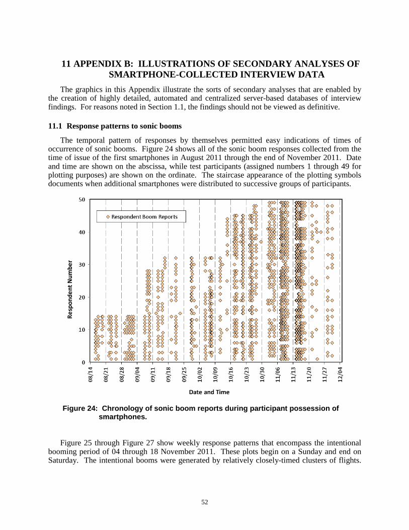
52

11 APPENDIX B: ILLUSTRATIONS OF SECONDARY ANALYSES OFSMARTPHONE-COLLECTED INTERVIEW DATA

The graphics in this Appendix illustrate the sorts of secondary analyses that are enabled bythe creation of highly detailed, automated and centralized server-based databases of interviewfindings. For reasons noted in Section 1.1, the findings should not be viewed as definitive.

11.1 Response patterns to sonic booms

The temporal pattern of responses by themselves permitted easy indications of times ofoccurrence of sonic booms. Figure 24 shows all of the sonic boom responses collected from thetime of issue of the first smartphones in August 2011 through the end of November 2011. Dateand time are shown on the abscissa, while test participants (assigned numbers 1 through 49 forplotting purposes) are shown on the ordinate. The staircase appearance of the plotting symbolsdocuments when additional smartphones were distributed to successive groups of participants.

Figure 24: Chronology of sonic boom reports during participant possession ofsmartphones.

Figure 25 through Figure 27 show weekly response patterns that encompass the intentionalbooming period of 04 through 18 November 2011. These plots begin on a Sunday and end onSaturday. The intentional booms were generated by relatively closely-timed clusters of flights.

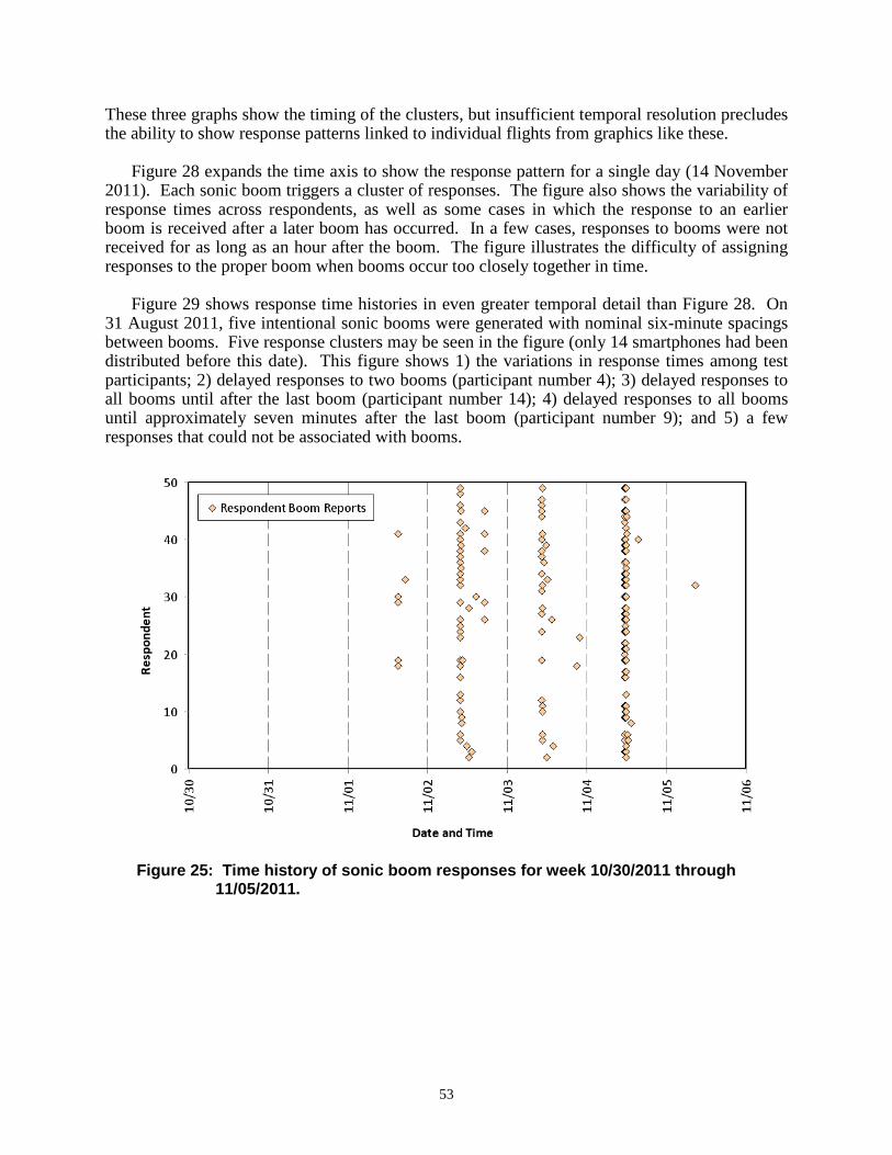
53

These three graphs show the timing of the clusters, but insufficient temporal resolution precludesthe ability to show response patterns linked to individual flights from graphics like these.

Figure 28 expands the time axis to show the response pattern for a single day (14 November2011). Each sonic boom triggers a cluster of responses. The figure also shows the variability ofresponse times across respondents, as well as some cases in which the response to an earlierboom is received after a later boom has occurred. In a few cases, responses to booms were notreceived for as long as an hour after the boom. The figure illustrates the difficulty of assigningresponses to the proper boom when booms occur too closely together in time.

Figure 29 shows response time histories in even greater temporal detail than Figure 28. On31 August 2011, five intentional sonic booms were generated with nominal six-minute spacingsbetween booms. Five response clusters may be seen in the figure (only 14 smartphones had beendistributed before this date). This figure shows 1) the variations in response times among testparticipants; 2) delayed responses to two booms (participant number 4); 3) delayed responses toall booms until after the last boom (participant number 14); 4) delayed responses to all boomsuntil approximately seven minutes after the last boom (participant number 9); and 5) a fewresponses that could not be associated with booms.

Figure 25: Time history of sonic boom responses for week 10/30/2011 through11/05/2011.

54

Figure 26: Chronology of sonic boom responses for week 11/06/2011 through11/12/2011.

Figure 27: Chronology of sonic boom responses for week 11/13/2011 through11/20/2011.

55

Figure 28: Sonic boom response time history for 14 November 2011.

Figure 29: Response time history for a 1-1/2 hour period of intentional sonic boomson 31 August 2011.

56

11.2 Response latencies and implications

Section 4.1, along with Figure 15 and Figure 16, showed distribution density functions forresponse latencies following a sonic boom. Figure 30 (below) shows the cumulative distributionof latencies within an hour following a boom. The slow asymptotic rise to 100 percent afterapproximately 90 percent of respondents had completed interviews is noteworthy.

Figure 31 displays only the first 15 minutes of the data of Figure 30. This presentationpermits greater detail to be seen in the length of time required to acquire various percentages ofcompleted interviews. For example, just over forty seconds was required to complete half of theinterviews. Within about six minutes of the occurrence of a boom, 90 percent of the responseswere completed, and a little more than three minutes was required to collect 80 percent of theresponses. However, nearly 1700 seconds (28 minutes) was required to collect 95 percent of theresponses, an increase of 22 minutes beyond the 90 percent point.

The findings presented in these two figures bear on the ability to unambiguously assign theproper doses to responses based on the length of inter-boom intervals. They also raise questionsabout whether delayed reactions are reported with the same accuracy as prompt reactions.

0%

10%

20%

30%

40%

50%

60%

70%

80%

90%

100%

0 300 600 900 1200 1500 1800 2100 2400 2700 3000 3300 3600

Response Latency (seconds)

Cu

mla

tiv

eP

erc

en

to

fO

bs

erv

ati

on

s

Figure 30: Cumulative distribution function of observed response latencies as longas an hour following a boom.

57

0%

10%

20%

30%

40%

50%

60%

70%

80%

90%

100%

0 60 120 180 240 300 360 420 480 540 600 660 720 780 840 900

Response Latency (seconds)

Cu

mla

tiv

eP

erc

en

to

fO

bse

rva

tio

ns

Figure 31: Cumulative distribution function of observed response latencies up to 15minutes following boom event.

11.3 Low battery conditions encountered by test participants

As configured and used in the present pilot test, the battery life of the Droid2 smartphonesthat were distributed to test participants was approximately 24 hours.29 In practice, this meantthat most smartphones had to be recharged every night.

Many of the test participants were familiar with earlier (that is, less capable but lower power)cell phones, which did not require daily recharging. Figure 32 plots the frequency with whichtest participants experienced low batteries. The abscissa indicates the number of low batteryfailures encountered during the 15-day test period. The largest number encountered by anyparticipant was 11. The ordinate shows the percentage of the 49-person participant poolexperiencing a given number of failures. For example, 13 participants (or 27%) neverexperienced a single low battery failure. Another 11 (22%) experienced just one such failure,and so on. The median number of shutdowns attributable to low battery power is between oneand two.

29 Battery life depended not only on power use for the application software developed for the current pilot test, butalso on the use of smartphones for other purposes. Thus, battery life varied greatly among test participants whomade little use of their smartphones for purposes other than reporting sonic booms, and those who used theirsmartphones extensively for other power-intensive uses (e.g., map and navigation applications and imageprocessing), and/or made heavy use of their smartphones for social media, file downloading, texting, calling, andother miscellaneous applications.

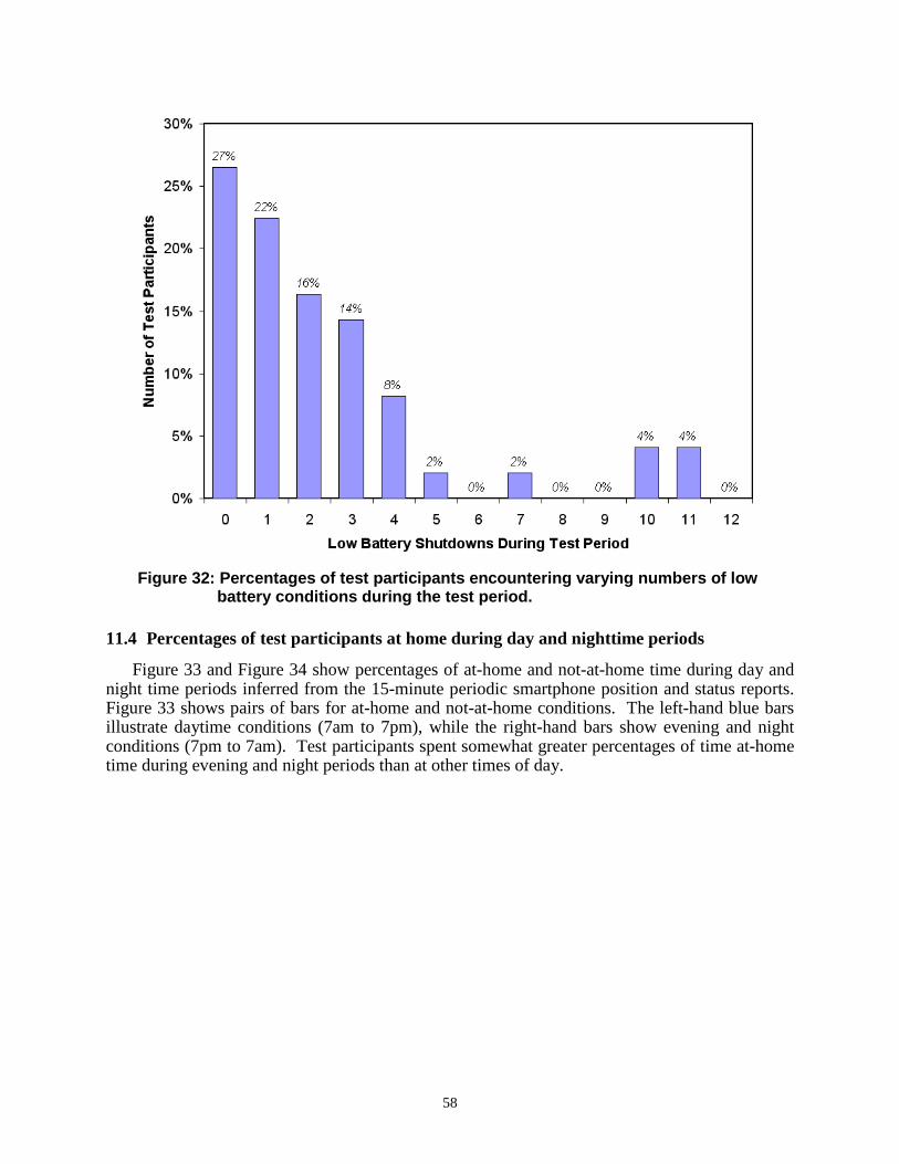
58

Figure 32: Percentages of test participants encountering varying numbers of lowbattery conditions during the test period.

11.4 Percentages of test participants at home during day and nighttime periods

Figure 33 and Figure 34 show percentages of at-home and not-at-home time during day andnight time periods inferred from the 15-minute periodic smartphone position and status reports.Figure 33 shows pairs of bars for at-home and not-at-home conditions. The left-hand blue barsillustrate daytime conditions (7am to 7pm), while the right-hand bars show evening and nightconditions (7pm to 7am). Test participants spent somewhat greater percentages of time at-hometime during evening and night periods than at other times of day.

59

Figure 33: Comparison of at-home status between daytime and evening/nighttimeperiods

Figure 34 presents participant at-home status in greater detail. This figure shows thepercentage of time test participants were at home by hour of the day. Each data point shows theaverage across all smartphone status reports during the weekdays and weekend days of the testperiod. The data are dichotomized by weekday (circles) and weekend (squares) since all sonicbooms during the test period were observed between Monday and Friday. The vertical linesbracket the period of the day during which sonic booms (intended and adventitious) wereobserved.

The diurnal pattern shows greater variability over the weekend than during weekdays. At notime did the percentage of at-home participants drop below 80 percent during weekdays. Thecomparable minimal value for weekends was 75 percent.

11.5 Questionnaire completion rates

The percentages of respondents answering each of the interview questions are shown inFigure 35. (The figure numbers identified in the caption refer to questionnaire items shown inearlier figures in this report.) The figure shows two set of bars. The leftmost bar of each pairindicates the percentage of respondents initiating an interview who also answered eachquestionnaire item.

Questions 1 through 5 were asked of every respondent without any conditionality. Thefigure shows that all respondents answered these questions. Question 6 was asked only to the1543 respondents who answered “Indoors” in response to Question 5. Of these 1543respondents, all answered Question 6. Question 6 asked if participants had noticed rattle. Atotal of 743 participants responded in the affirmative. Question 7 asked whether those 743 were

60

bothered or annoyed by rattle. All 743 participants answered that question, of whom 273responded that the rattle was annoying in some degree. Question 8 was posed to those 273, whowere asked about their degree of annoyance with the rattle. All 273 (100%) answered the lastquestion.

These results clearly indicate that test participants were able to follow the on-screendirections and were engaged enough by the brief questionnaire to follow through to completionall questions that were asked of them.

Figure 34: Participant at-home status by hour of day, for weekday/weekend periods.

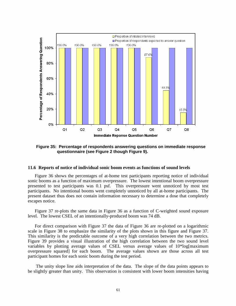
61

Figure 35: Percentage of respondents answering questions on immediate responsequestionnaire (see Figure 2 though Figure 9).

11.6 Reports of notice of individual sonic boom events as functions of sound levels

Figure 36 shows the percentages of at-home test participants reporting notice of individualsonic booms as a function of maximum overpressure. The lowest intentional boom overpressurepresented to test participants was 0.1 psf. This overpressure went unnoticed by most testparticipants. No intentional booms went completely unnoticed by all at-home participants. Thepresent dataset thus does not contain information necessary to determine a dose that completelyescapes notice.

Figure 37 re-plots the same data in Figure 36 as a function of C-weighted sound exposurelevel. The lowest CSEL of an intentionally-produced boom was 74 dB.

For direct comparison with Figure 37 the data of Figure 36 are re-plotted on a logarithmicscale in Figure 38 to emphasize the similarity of the plots shown in this figure and Figure 37.This similarity is the predictable outcome of a very high correlation between the two metrics.Figure 39 provides a visual illustration of the high correlation between the two sound levelvariables by plotting average values of CSEL versus average values of 10*log[maximumoverpressure squared] for each boom. The average values shown are those across all testparticipant homes for each sonic boom during the test period.

The unity slope line aids interpretation of the data. The slope of the data points appears tobe slightly greater than unity. This observation is consistent with lower boom intensities having

62

greater proportions of low frequency spectral content below 20 Hz than higher boom intensities,a portion of the spectrum deemphasized by the C-weighting function.

Figure 36: Percentages of at-home participants noticing sonic booms as a functionof maximum boom overpressure.

63

Figure 37: Percentages of at-home participants noticing sonic booms as a functionof C-weighted sound exposure level.

Figure 38: Percentages of at-home participants noticing sonic booms as a functionof maximum boom overpressure (logarithmic scale)

64

Figure 39: Observed relationship between C-weighted sound exposure level andsquare of maximum overpressure (dashed line is unity slope)

11.7 Analysis of responses to question about individually memorable booms

One question in the end-of-day interview asked “Was any one particular sonic boom that younoticed today much more annoying than any of the others?” The question was asked toinvestigate the contributions of individual booms to the annoyance of cumulative exposure, andwhether annoyance judgments can be modeled as an energy integration process. It was alsoasked to investigate whether such a self-report could be associated with objective measures ofsingle-event sound levels.

Figure 40 plots the percentage of respondents who answered “Yes” as a function of the day’sC-weighted day-night average sound level exposure to sonic booms. Open circles identifypercentages of respondents who reported hearing one or fewer booms, and thus were not asked ifone boom was more annoying than others. This percentage declines with increasing CDNL,suggesting that days of higher CDNL may have included greater numbers of individuallymemorable booms in the present dataset.

Among respondents who reported noticing more than one boom, the percentages whobelieved that one boom was more annoying than others are plotted as solid red squares in Figure40. This percentage tends to increase with CDNL.

65

0%

10%

20%

30%

40%

50%

60%

70%

80%

90%

100%

35 40 45 50 55 60 65 70 75

CDNL (dB)

Perc

en

tag

eo

fR

eso

nd

en

ts

Recalled hearing only 1 or fewer booms

Yes, one more annoying than others

Figure 40: Relationship between percent of respondents reporting one boom to belouder than all others for the day and CDNL.

Figure 41 summarizes a more direct analysis of responses to the question. This figure plotsthe relationship between the percentage of respondents describing one boom as more annoyingthan all others (ordinate) and the CSEL difference between the highest and second highest boom(abscissa)30, 31. The responses seem to cluster into two sets: 1) those in the 1 to 2 decibeldifference range, whose corresponding percentages exceed 15 percent, and 2) the remaining lowCSEL difference points and those with CSEL differences greater than 2 decibels.

The high percentage data points in the 1 to 2 decibel range seem less than plausible if allrespondents were exposed to all booms during the day. However, if some respondents were notat home for all booms, then perhaps of the booms they did hear, one stood out above the others.A more detailed analysis would be required at the individual event level to more fully understandthis observation.

Figure 42 re-plots the data points of Figure 41 by showing as open plotting symbols thehigh-percentage / low CSEL difference points discussed above. The remaining filled plottingsymbols form a trend of increasing percent of respondents noticing a single annoying boom withincreasing CSEL difference between the two highest sound level booms. The slope of therelationship appears to be approximately 3 percent increase in noticeability per decibel ofdifference.

30 The data points stack in a vertical straight line because the sound level data was reported to the nearest wholedecibel.31 Note that from Figure 39 this relationship would differ little if the boom exposure were expressed in terms ofboom overpressures.

66

28.6%

37.5%

18.9%

38.9%

14.8%

48.6%

60.5%

66.7%

23.8%

8.3%

0%

10%

20%

30%

40%

50%

60%

70%

80%

90%

100%

0 2 4 6 8 10 12 14

CSELmax - CSELnext-highest (dB)

Pe

rce

nta

ge

of

Res

on

de

nts

Re

po

rtin

gO

ne

Ev

en

tM

ore

An

no

yin

gth

an

Oth

ers

Figure 41: Relationship between percent of respondents reporting one boom louderthan others and CSEL difference between loudest and next loudest boom.

0%

10%

20%

30%

40%

50%

60%

70%

80%

90%

100%

0 2 4 6 8 10 12 14

CSELmax - CSELnext-highest (dB)

Pe

rce

nta

ge

of

Re

so

nd

en

tsR

ep

ort

ing

On

eE

ve

nt

Mo

re

An

no

yin

gth

an

Oth

ers

~ 3.1% per decibel

Figure 42: Relationship between percent of respondents reporting one boom louderthan others and CSEL difference between loudest and next loudest boom(with fit line).

67

Figure 43 shows the data of Figure 42 in a slightly different manner. The ordinate is thesame in both figures, as are the percentages for each plotting symbol. However, the abscissa inFigure 43 plots the energy difference between the boom of highest CSEL and that of all otherbooms combined by subtracting the CDNL of all but the highest level boom from that of thehighest. The same days shown with open plotting symbols in Figure 42 are also shown as openplotting symbols in this figure. In other words, the open plotting symbols in Figure 43 alsoindicate days on which there was very little difference in single event levels between the highestand second highest booms. A similar trend, also of approximately 3 percent per decibel slope, isevident. Visually, the residuals about the trend lines in the two figures seem indistinguishablefrom one another, so it is not clear from this limited data set whether one predictor performsbetter than the other.

Taken together, the patterns apparent in Figure 40 through Figure 43 suggest that people aresensitive to unusually annoying individual booms, even if they do not occur in close temporalproximity to other booms. This, in turn, suggests the possibility of tailoring exposure schedulesin future studies to permit investigations of the manner in which people integrate the annoyanceof individual booms into their estimates of the annoyance of cumulative exposure.

0%

10%

20%

30%

40%

50%

60%

70%

80%

90%

100%

-7 -5 -3 -1 1 3 5 7

CDNLmax - CDNLremaining (dB)

Pe

rce

nta

ge

of

Res

on

den

tsR

ep

ort

ing

On

eE

ve

nt

Mo

re

An

no

yin

gth

an

Oth

ers

~ 3.7% per decibel

Figure 43: Relationship between percent of respondents reporting one boom to belouder than all others for the day and the difference in CDNLs between thatof the loudest boom and all the rest (with fit line).

11.8 Reports of annoyance of individual sonic boom events as functions of sound levels

Figure 44 illustrates the degrees of annoyance associated with CSEL values for individualbooms. In general, greater percentages of test participants describe themselves as at least slightly

68

annoyed at lower CSEL values than the percentages of those who describe themselves as at leastmoderately annoyed. Conversely, higher CSEL values are generally required for test participantsto describe themselves as “very” or “extremely” (“highly”) annoyed than for test participants todescribe themselves as at least moderately annoyed by sonic booms.

0%

10%

20%

30%

40%

50%

60%

70%

70 80 90 100 110

Boom CSEL (dB)

Pe

rce

nt

An

no

ye

db

yB

oo

m

Slightly+ Annoyed

Moderately+ Annoyed

Highly Annoyed

Figure 44: Percentages of at-home test participants reporting three differentdegrees of annoyance to sonic booms as a function of C-weighted soundexposure level.

11.9 Reports of startle associated with individual sonic boom events as functions of soundlevels

Figure 45 shows a clear trend of increasing percentages of test participants reporting startlewith increasing sound exposure levels of sonic booms. Reports of notice of rattle associated withindividual sonic boom events as functions of sound levels.

Figure 46 shows a clear trend of increasing percentages of test participants reporting noticeof rattle with increasing sound exposure levels of sonic booms.

69

0%

10%

20%

30%

40%

50%

60%

70%

70 80 90 100 110

Boom CSEL (dB)

Pe

rce

nt

Sta

rtle

db

yB

oo

m

Figure 45: Percentages of at-home test participants reporting startle to sonic boomsas a function of C-weighted sound exposure level.

0%

10%

20%

30%

40%

50%

60%

70%

70 80 90 100 110

Boom CSEL (dB)

Pe

rcen

tN

oti

cin

gR

att

le

Figure 46: Percentages of at-home test participants noticing rattle as a function ofC-weighted sound exposure level.

REPORT DOCUMENTATION PAGEForm Approved

OMB No. 0704-0188

2. REPORT TYPE

Contractor Report 4. TITLE AND SUBTITLE

Pilot Test of a Novel Method for Assessing Community Response to Low-Amplitude Sonic Booms

5a. CONTRACT NUMBER

NNL10AA19C

6. AUTHOR(S)

Fidell, Sanford; Horonjeff, Richard D.; Harris, Michael

7. PERFORMING ORGANIZATION NAME(S) AND ADDRESS(ES)

NASA Langley Research Center Hampton, Virginia 23681-2199

9. SPONSORING/MONITORING AGENCY NAME(S) AND ADDRESS(ES)

National Aeronautics and Space AdministrationWashington, DC 20546-0001

8. PERFORMING ORGANIZATION REPORT NUMBER

10. SPONSOR/MONITOR'S ACRONYM(S)

NASA

13. SUPPLEMENTARY NOTES

Langley Technical Monitor: Kevin P. Shepherd

12. DISTRIBUTION/AVAILABILITY STATEMENTUnclassified - UnlimitedSubject Category 71Availability: NASA CASI (443) 757-5802

19a. NAME OF RESPONSIBLE PERSON

STI Help Desk (email: help@sti.nasa.gov)

14. ABSTRACT

A pilot test of a novel method for assessing residents’ annoyance to sonic booms was performed. During a two-week period, residents of the base housing area at Edwards Air Force Base provided data on their reactions to sonic booms using Smartphone-based interviews. Noise measurements were conducted at the same time. The report presents information about data collection methods and about test participants’ reactions to low-amplitude sonic booms. The latter information should not be viewed as definitive for several reasons. It may not be reliably generalized to the wider U.S. residential population (because it was not derived from a representative random sample) and the sample itself was not large.

15. SUBJECT TERMS

Aircraft Noise; Community Response; Sonic Boom

18. NUMBER OF PAGES

72

19b. TELEPHONE NUMBER (Include area code)

(443) 757-5802

a. REPORT

U

c. THIS PAGE

U

b. ABSTRACT

U

17. LIMITATION OF ABSTRACT

UU

Prescribed by ANSI Std. Z39.18Standard Form 298 (Rev. 8-98)

3. DATES COVERED (From - To)

5b. GRANT NUMBER

5c. PROGRAM ELEMENT NUMBER

5d. PROJECT NUMBER

5e. TASK NUMBER

5f. WORK UNIT NUMBER

984754.02.07.07.18.03

11. SPONSOR/MONITOR'S REPORT NUMBER(S)

NASA/CR-2012-217767

16. SECURITY CLASSIFICATION OF:

The public reporting burden for this collection of information is estimated to average 1 hour per response, including the time for reviewing instructions, searching existing data sources, gathering and maintaining the data needed, and completing and reviewing the collection of information. Send comments regarding this burden estimate or any other aspect of this collection of information, including suggestions for reducing this burden, to Department of Defense, Washington Headquarters Services, Directorate for Information Operations and Reports (0704-0188), 1215 Jefferson Davis Highway, Suite 1204, Arlington, VA 22202-4302. Respondents should be aware that notwithstanding any other provision of law, no person shall be subject to any penalty for failing to comply with a collection of information if it does not display a currently valid OMB control number.PLEASE DO NOT RETURN YOUR FORM TO THE ABOVE ADDRESS.

1. REPORT DATE (DD-MM-YYYY)

09 - 201201-