NALYSIS AND PREDICTION OF DEFORMING 3D SHAPES USING ...

ANALYSIS AND PREDICTION OF DEFORMING 3D SHAPES USINGORIENTED BOUNDING BOXES AND LSTM AUTOENCODERS

PREPRINT ACCEPTED AT THE 29TH INTERNATIONAL CONFERENCE ON ARTIFICIAL NEURAL NETWORKS

Sara HahnerFraunhofer Center for Machine Learning and SCAI

[email protected]

Rodrigo Iza-TeranFraunhofer Center for Machine Learning and SCAI

[email protected]

Jochen GarckeFraunhofer Center for Machine Learning and SCAI

University of [email protected]

August 14, 2020

ABSTRACT

For sequences of complex 3D shapes in time we present a general approach to detect patterns fortheir analysis and to predict the deformation by making use of structural components of the com-plex shape. We incorporate long short-term memory (LSTM) layers into an autoencoder to createlow dimensional representations that allow the detection of patterns in the data and additionally de-tect the temporal dynamics in the deformation behavior. This is achieved with two decoders, onefor reconstruction and one for prediction of future time steps of the sequence. In a preprocessingstep the components of the studied object are converted to oriented bounding boxes which capturethe impact of plastic deformation and allow reducing the dimensionality of the data describing thestructure. The architecture is tested on the results of 196 car crash simulations of a model with 133different components, where material properties are varied. In the latent representation we can de-tect patterns in the plastic deformation for the different components. The predicted bounding boxesgive an estimate of the final simulation result and their quality is improved in comparison to differentbaselines.

Keywords LSTM Autoencoder · 3D Shape Deformation Analysis · CAE Analysis · 3D Time Series

1 Introduction

Deforming 3D shapes that can be subdivided into components can be found in many different areas, for example crashanalysis, structure, and material testing, or moving humans and animals that can be subdivided into body parts. Thedata can be especially challenging since it has a temporal and a spatial dimension that have to be considered jointly. Inparticular, we consider shape data from Computer Aided Engineering (CAE), where numerical simulations play a vitalrole in the development of products, as they enable simpler, faster, and more cost-effective investigations of systems.If the 3D shape is complex, the detection of patterns in the deformation, called deformation modes in CAE (figure 1),speeds up the analysis.

While deformation modes are dependent on model parameters, their behavior is accessible, albeit tediously, uponmanifestation when having access to the completed simulation run. In practice this detection of deformation modes isbased on error-prone supervision of a non-trivial, hand-selected subset of nodes in critical components.

In general, simulation results contain abundant features and are therefore high dimensional and unwieldy, whichmakes comparative analysis difficult. Intuitively, the sampled points describing the component are highly correlated,not only in space but also over time. This redundancy in the data invites further analysis via feature learning, reducingunimportant information in space as well as time and thus dimensionality. The low dimensional features capture

arX

iv:2

009.

0378

2v1

[cs

.CV

] 3

1 A

ug 2

020


Mode A: Mode B:

Figure 1: Deformation modes of left front beams in the example car model.

Time: 1, . . . , TIN

OBB Representation

LSTMAutoencoder

TIN + 1, . . . , TFIN

Prediction

Time-independenthidden representation

Mode B

Mode A

Mode A

Figure 2: Analysis and Prediction of Deforming Shapes. Preprocess the first TIN time steps of simulation data byoriented bounding boxes, apply an LSTM autoencoder which predicts the future time steps and creates a hiddenrepresentation representing the deformation over time. Finally, the deformation modes from figure 1 can be detectedin the hidden representations.

distinguishing characteristics to detect the deformation modes. As soon as the deformation of a component is attributedto a deformation mode, there is little variance regarding its further course in the simulation. This motivates the in-situdetection, that is during the simulation, of deformation modes; we can then interrupt the simulation and anticipatetargeted changes to the model parameters.

For the in-situ analysis of deforming shapes, we propose the application of an LSTM autoencoder trained on acomponent-wise shape representation by oriented bounding boxes instead of directly on the 3D data points (or meshes)describing the shapes. Motivated by an architecture with two decoders that stems from unsupervised video predic-tion [26], we choose a composite LSTM autoencoder that is specialized on handling time sequences and can bothreconstruct the input and predict the future time steps of a sequence. It creates an additional low dimensional hiddenor latent representation which after successful training represents the features of the input time sequences and allowsits reconstruction and prediction. In this case the features encode the distinctive characteristics of the component’sdeformation. Figure 2 illustrates the process.

The research goals can be summarized as a) the definition of a distinguishing and simple shape representation forstructural components of a complex model, b) the in-situ detection of patterns in the deformation behavior, and c) thein-situ prediction of structural component positions at future time steps.

Further on in section 2, we give an introduction to simulation data, which we choose as example data, its characteristicsand limitations. In section 3, we present oriented bounding boxes, the selected shape representation for structuralcomponents, followed by the definition of the LSTM autoencoder in section 4. In section 5, we discuss related workon machine learning for simulations. Results on a car crash simulation are presented in section 6.

2 Simulation Data and Their Characteristics

As an example for a deforming shape over time, we consider 3D (surface) meshes, which are decomposed into struc-tural components. A numerical simulation approximately computes the deformation of the underlying object on the

2


basis of physical relations. For each simulation, model, material, or environment parameters might be varied as wellas the geometry of components or their connections. The output of a simulation are the positions of the mesh pointsat different times and point-wise values of physical quantities. While a large variety of deformation processes is ob-served per component, they result in a small number of meaningful patterns, called deformation modes. In figure 1two distinct deformation modes of two structural components during a car crash can be observed.

Car crash simulations are a complex example. The mesh sizes for the car models can be large, the number anddiversity of the input parameters is high and the behavior is nonlinear. Furthermore, the calculations need to havea high degree of precision, because the evaluation of the passenger’s safety is based on the simulation outputs, i.e.plastic deformation, strain, and rupture. The stored simulations nowadays contain detailed information for up to twohundred time steps and more than ten million nodes. Due to the large computational costs of one simulation, for onemodel there are generally less than 500 different runs.

From simulation run to simulation run the input parameters are modified to achieve the design goals, e.g. crash safety,weight, or performance. In the beginning, the goal is the broad understanding of deformation behavior by applyingmajor changes to the model. In later design stages a fine tuning is done and tests address some issues that have not beencaptured in early stages. We present an approach that analyzes the whole car as a multi-body object under dynamicdeformation. Therefore, it is applied at an early design stage where the broad deformation behavior and componentinteraction has to be understood.

Challenges in the Analysis

Because of the high data complexity, the relatively low number of samples, and fatal consequences of wrong resultson the passenger’s safety, many data analysis methods cannot be applied directly. Furthermore, a full prediction ofthe complex simulation results, including detailed deformation or strains, only based on the input parameters is errorprone and critical for the purpose of precise parameter selections and the understanding of detailed physical behavior.Existing methods create a surrogate model given some input parameters, see e.g. [27]. Others show how deformationmodes depend on input parameters by using visualizations in low dimensional representations without defining anexplicit surrogate model [15, 30].

We do not want to base our analysis on input parameters, but present a more general approach that concentrates ongeneral deformation behavior. By applying an in-situ analysis and an estimation of the deformation in the future timesteps, we provide information that allows a faster selection of new model parameters in the development process.

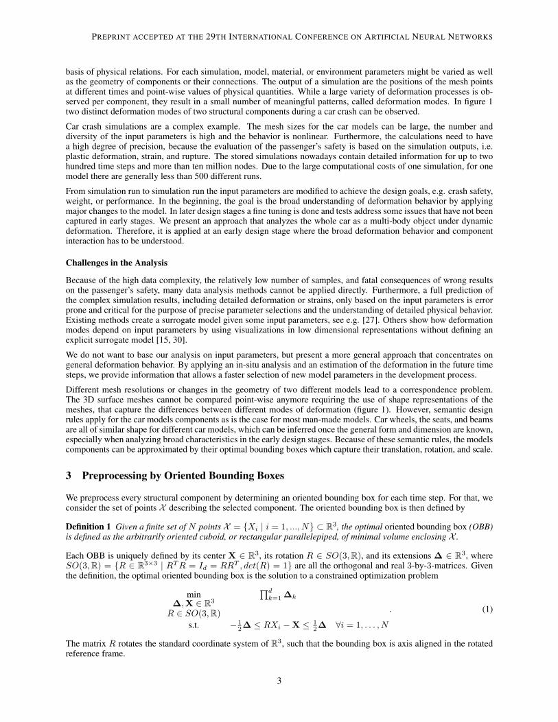
Different mesh resolutions or changes in the geometry of two different models lead to a correspondence problem.The 3D surface meshes cannot be compared point-wise anymore requiring the use of shape representations of themeshes, that capture the differences between different modes of deformation (figure 1). However, semantic designrules apply for the car models components as is the case for most man-made models. Car wheels, the seats, and beamsare all of similar shape for different car models, which can be inferred once the general form and dimension are known,especially when analyzing broad characteristics in the early design stages. Because of these semantic rules, the modelscomponents can be approximated by their optimal bounding boxes which capture their translation, rotation, and scale.

3 Preprocessing by Oriented Bounding Boxes

We preprocess every structural component by determining an oriented bounding box for each time step. For that, weconsider the set of points X describing the selected component. The oriented bounding box is then defined by

Definition 1 Given a finite set of N points X = {Xi | i = 1, ..., N} ⊂ R3, the optimal oriented bounding box (OBB)is defined as the arbitrarily oriented cuboid, or rectangular parallelepiped, of minimal volume enclosing X .

Each OBB is uniquely defined by its center X ∈ R3, its rotation R ∈ SO(3,R), and its extensions ∆ ∈ R3, whereSO(3,R) = {R ∈ R3×3 | RTR = Id = RRT , det(R) = 1} are all the orthogonal and real 3-by-3-matrices. Giventhe definition, the optimal oriented bounding box is the solution to a constrained optimization problem

min∆,X ∈ R3

R ∈ SO(3,R)

∏dk=1 ∆k

s.t. − 12∆ ≤ RXi −X ≤ 1

2∆ ∀i = 1, . . . , N

. (1)

The matrix R rotates the standard coordinate system of R3, such that the bounding box is axis aligned in the rotatedreference frame.

3


We employ the HYBBRID algorithm [4] to approximate the boxes, since the exact algorithm has cubic runtime in thenumber of points in the convex hull of X [21]. Also, the quality of the approximation by fast principal componentanalysis (PCA) based algorithms is limited [6]. However, we need the oriented bounding boxes to fit tightly, which iswhy we adapted the HYBBRID algorithm for the OBB approximations of time sequences.

Adapted HYBBRID Algorithm

A redefinition of (1) as in [4] allows the problem’s analysis as an unconstrained optimization over SO(3,R)min

R∈SO(3,R)f(R),

where f(R) is the volume of the axis aligned bounding box of the point set X rotated by R. Since the function is notdifferentiable, a derivative-free algorithm combining global search by a genetic algorithm [8, 14] (exploration) andlocal search by the Nelder-Mead simplex algorithm [20] (exploitation) to find the rotation matrix R∗ ∈ SO(3,R) thatminimizes f is introduced in [4], where a detailed description of the algorithm can be found.

By utilizing the best rotation matrix from the previous time step of the same component, we can give a good initialguess to the algorithm. This improves the quality of the approximations and reduces the runtime by 30% in comparisonto the original HYBBRID algorithm.

Information Retrieval from OBBs

The oriented bounding boxes further allow consideration of translation, rotation, and scale of the car componentsindividually. The rigid transform of a component, composed of its translation and rotation, is normally estimated usinga few fixed reference points for each component [28] and might be subtracted from the total deformation for analysis.Nevertheless, the quality of this rigid transform estimation depends highly on the hand selected reference points. Whenutilizing oriented bounding boxes the use of reference points is not necessary any more, since the HYBBRID algorithmoutputs the rotation matrix R∗. This allows detecting interesting characteristics in the components deformations thatare not translation or rotation based.

4 LSTM Autoencoders

Autoencoders are a widely used type of neural network for unsupervised learning. They learn low dimensional char-acteristic features of the input that allow its recreation as well as possible. Therefore, the hidden or low dimensionalrepresentations should show the most relevant aspects of the data and classification tasks can generally be solved betterin the low dimensional space. Autoencoders stand out against other dimension reduction approaches, because the en-coder enables quick evaluation and description of the manifold, on which the hidden representations lie [9]. Therefore,a new data points embedding does not have to be obtained by interpolation.

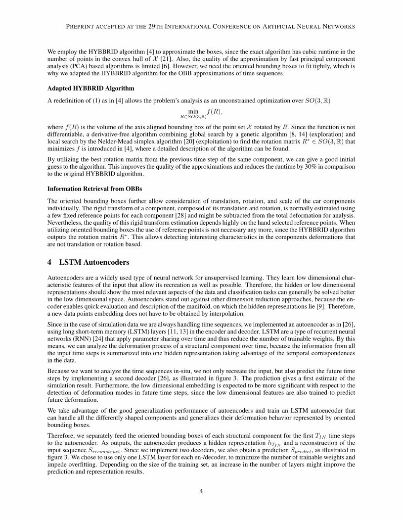
Since in the case of simulation data we are always handling time sequences, we implemented an autoencoder as in [26],using long short-term memory (LSTM) layers [11, 13] in the encoder and decoder. LSTM are a type of recurrent neuralnetworks (RNN) [24] that apply parameter sharing over time and thus reduce the number of trainable weights. By thismeans, we can analyze the deformation process of a structural component over time, because the information from allthe input time steps is summarized into one hidden representation taking advantage of the temporal correspondencesin the data.

Because we want to analyze the time sequences in-situ, we not only recreate the input, but also predict the future timesteps by implementing a second decoder [26], as illustrated in figure 3. The prediction gives a first estimate of thesimulation result. Furthermore, the low dimensional embedding is expected to be more significant with respect to thedetection of deformation modes in future time steps, since the low dimensional features are also trained to predictfuture deformation.

We take advantage of the good generalization performance of autoencoders and train an LSTM autoencoder thatcan handle all the differently shaped components and generalizes their deformation behavior represented by orientedbounding boxes.

Therefore, we separately feed the oriented bounding boxes of each structural component for the first TIN time stepsto the autoencoder. As outputs, the autoencoder produces a hidden representation hTIN

and a reconstruction of theinput sequence Sreconstruct. Since we implement two decoders, we also obtain a prediction Spredict, as illustrated infigure 3. We chose to use only one LSTM layer for each en-/decoder, to minimize the number of trainable weights andimpede overfitting. Depending on the size of the training set, an increase in the number of layers might improve theprediction and representation results.

4


ENCODERLSTM layer

Sin = {s1, s2, . . . , sTIN}

hTIN

low-dim representation: hTIN

1st DECODER LSTM layer 2nd DECODERLSTM layer

{h′1, h′2, . . . , h′TIN}

Feed forward layer F1

{h′TIN+1, . . . , h′TFIN

}

Feed forward layer F2

Sreconstruct = {o1, o2, . . . , oTIN} Spredict = {oTIN+1, . . . , oTFIN

}

Figure 3: LSTM autoencoder. The last hidden vector hTin of the encoder layer is utilized as the low dimensionalrepresentation, which is input to all the LSTM units of the decoders. By applying time independent feed forwardlayers to the hidden vectors h′• of each decoder, their size is reduced and the output sequences Sreconstruct andSpredict are created. The weights of the LSTM layers and F• are time independent.

5 Related Work

The analysis of car crash simulations has been studied with different machine learning techniques. For example,[1, 2, 10, 32] base their analysis on the finished simulation runs, whereas we focus on in-situ analysis of car crashsimulations.

Other recent works study analysis and prediction of car crash simulation data with machine learning under differentproblem definitions than in this work, for example the estimation of the result given the input parameters [12] orplausibility checks [25]. For a recent overview on the combination of machine learning and simulation see [23].

There are alternatives to oriented bounding boxes as low dimensional shape representations for 3D objects. The authorsof [15] construct low dimensional shape representations via a projection of mesh data onto an eigenbasis stemmingfrom a discrete Laplace Beltrami Operator. The data is then represented by the spectral coefficients. We have chosena simpler representation, that can also be applied to point clouds and allows a faster training.

The majority of works about neural networks for geometries extend convolutional neural networks on non-euclideanshapes, including graphs and manifolds. The works in [3, 17, 19] present extensions of neural networks via the com-putation of local patches. Nevertheless, the networks are applied to the 3D meshes directly and are computationallyexpensive, when applied for every time step and component of complex models.

Based on the shape deformation representation by [7], recent works studied generative modeling of meshes for 3Danimation sequences via bidirectional LSTM network [22] or variational autoencoder [29]. The shape representationyields good results, however, it solves an optimization problem at each vertex and requires identical connectivity overtime. The architectures are tested on models of humans with considerably fewer nodes, which is why computationalissues seem likely for the vertex-wise optimization problem.

6 Experiments

We evaluated the introduced approach on a frontal crash simulation of a Chevrolet C2500 pick-up truck1. The dataset consists of nsimulations = 196 completed simulations2 of a front crash (see figure 4), using the same truck, butwith different material characteristics, which is a similar setup to [2]. For 9 components (the front and side beams andthe bumper parts) the sheet thickness has been varied while keeping the geometry unchanged. From every simulationwe select TFIN = 31 equally distributed time steps and use TIN = 12 time steps for the input to the in-situ analysis,which is applied to 133 structural components represented by oriented bounding boxes. That means, when detecting a

1from NCAC http://web.archive.org/web/*/www.ncac.gwu.edu/vml/models.html2computed with LS-DYNa http://www.lstc.com/products/ls-dyna

5

http://web.archive.org/web/*/www.ncac.gwu.edu/vml/models.html

http://www.lstc.com/products/ls-dyna


Table 1: Structure of the composite LSTM autoencoder with two decoders for reconstruction and prediction. Thebullets • reference the corresponding batch size.

Layer Output Shape Param. Connected toInput (•, TIN , 24) 0

LSTM 1 (•, 24) 4704 InputRepeat Vector 1 (•, TIN , 24) 0 LSTM 1Repeat Vector 2 (•, TFIN − TIN , 24) 0 LSTM 1

LSTM 2 (•, TIN , 256) 287744 Repeat Vector 1LSTM 3 (•, TFIN − TIN , 256) 287744 Repeat Vector 2

Fully Connected 1 (•, TIN , 24) 6168 LSTM 2Fully Connected 2 (•, TFIN − TIN , 24) 6168 LSTM 3

Figure 4: Snapshot and bounding box representation of the example car model at TIN = 12 (bottom view). The fourbeams from figure 2 are colored.

bad simulation run after TIN of TFIN time steps the design engineer can save 60% of the simulation time. The impactat TIN = 12 is visualized in figure 4. At this time most of the deformation and energy absorption took place in theso-called crumble zone at the front of the car.

The data is normalized to zero mean for each of the three dimensions and standard deviation one over all the di-mensions. Using all 133 components from 100 training samples we train the network3 for 150 epochs with adaptivelearning rate optimization algorithm [16]. We minimize the mean squared error between true and estimated boundingboxes over time, summing up the error for reconstruction and prediction decoder as well as for the components. Theremaining 96 simulations are testing samples.

Because of the limited number of training samples, we tried to minimize the number of hidden neurons while main-taining the quality, to reduce the possibility of overfitting and speed up the training. We observed that the result isstable with respect to the number of hidden neurons, which we finally set to 24 for the encoder and 256 for the de-coders. This leads to a total of 592,528 trainable weights, which are distributed over the layers as listed in table 1. Thetraining has a runtime of 36 seconds for one epoch on a CPU with 16 cores.

6.1 Prediction of Components’ Deformations during a Crash Test

The predicted oriented bounding boxes give an estimate after TIN time steps for the result of simulation S afterwards.For comparison, we define two baselines using a nearest neighbor search, where the prediction of S is estimated bythe future time steps of another simulation S′, which is either the corresponding simulation for the nearest neighbor ofS in the input sequences or in the input parameter space. We compare the results by their mean squared error which isalso used for training. Note that an interpolation has not been chosen for comparison, because interpolated rectangularboxes can have any possible shape.

The prediction error of our method is 38% lower than a prediction based on nearest neighbor search in the inputparameter space and 16% lower than a prediction using the nearest neighbor of the training input sequences, seetable 2. We also compare the LSTM composite autoencoder to a simple RNN composite autoencoder, to evaluate theuse of the LSTM layers in comparison to a different network architecture. When using the same number of hiddenweights for the simple RNN layer in the encoder and the decoders, the prediction error is higher than for the LSTMAutoencoder. This indicates, that the LSTM layers better detect the temporal correspondence in the time sequences.Additionally, the results depending on random initial weights are stable, which is demonstrated by the low standarddeviation of the error.

3implemented in Keras [5], no peephole connections

6


Table 2: Mean Squared Errors (×10−4) on testing samples for different prediction methods applied to oriented bound-ing boxes. For methods depending on random initialization, mean and standard deviation of 5 training runs are listed.

Method Test-MSE STDNearest neighbor in parameter space 13.34 -Nearest neighbor in input sequences 6.13 -Composite RNN autoencoder 5.80 0.095Composite LSTM autoencoder 5.14 0.127

Figure 5: Embedded hidden representations for all simulations and seven structural components, that manifest thedeformation modes from figure 1. The two different patterns for each of the selected structural components areillustrated in the same color with different intensity, the corresponding component on the right in the matching color.

We observe an improvement in the orthogonality between the faces of the rectangular boxes over time for both theprediction and reconstruction output of the LSTM layers. The LSTM layers recognize the conditions on the rectangularshape and implicitly enforce it in every output time step. Note, the network generalizes well to the highly differentsizes and shapes of 133 different structural components, whose oriented bounding boxes are illustrated in figure 4.

6.2 Clustering of the Deformation Behavior

The LSTM autoencoder does not only output a prediction, but also a hidden low dimensional representation. Itcaptures the most prominent and distinguishing features of the data, because only based on those the prediction andreconstruction are calculated. Its size corresponds to the number of hidden neurons in the encoder. Hence, our networkreduces the size of the 24×TIN -dimensional input to 24. The hidden representation summarizes the deformation overtime, which is why we obtain one hidden representation for the whole sequence of each structural component andsimulation.

In the case of car crash simulations we are especially interested in patterns in the plastic deformation to detect plasticstrain and material failure. Therefore, we add an additional preprocessing step for the analysis of deformation behavior.We subtract the rigid movement of the oriented bounding boxes, that means we translate the oriented bounding boxesto the origin and rotate them to the standard coordinate system (see section 3). In that way only the plastic deformationand strain are studied, but not induced effects in the rigid transform.

For a subset of components we visualize the 24-dimensional hidden representations in two dimensions with the t-SNEdimension reduction algorithm [18]. Figure 2 illustrates the embedding for the four frontal beams. We notice that thedeformation mode from figure 1 is clearly manifesting in the hidden representations of the left frontal beams.

When observing the hidden representations of other components, we can detect the pattern corresponding to thedeformation mode from figure 1 in other structural components, whose plastic deformation is seemingly influencedby the behavior of the left frontal beams. Even though the interaction between structural components is not fed to thenetwork, the components that are affected by the mode can be identified in figure 5.

7 Conclusion

We have presented a general approach for in-situ analysis and prediction of deforming 3D shapes by subdividing theminto structural components. The simple shape representation makes an analysis of complex models feasible and allowsthe detection of coarse deformation patterns. The method is applied successfully to a car crash simulation, estimates

7


the final position of the boxes to a higher quality than other methods, and speeds up the selection of new simulationparameters without having to wait for the final results of large simulations.

Although we have selected a relatively simple shape representation, the patterns can be reliably detected. In futurework, we plan to compare and combine the approach with other low dimensional shape representations and investigateother application scenarios, in particular in engineering. Apart from simulation data, our approach has more applica-tion areas, including the analysis and prediction of the movement of deformable articulated shapes, to which [31] givesan overview. The authors present data sets for human motion and pose analysis, on which the introduced approach canalso be applied.

References

[1] Bohn, B., Garcke, J., Griebel, M.: A sparse grid based method for generative dimensionality reduction of high-dimensional data. Journal of Computational Physics 309, 1–17 (2016)

[2] Bohn, B., Garcke, J., Iza-Teran, R., Paprotny, A., Peherstorfer, B., Schepsmeier, U., Thole, C.: Analysis of carcrash simulation data with nonlinear machine learning methods. Procedia Computer Science 18, 621–630 (2013)

[3] Bronstein, M.M., Bruna, J., LeCun, Y., Szlam, A., Vandergheynst, P.: Geometric deep learning: going beyondeuclidean data. IEEE Signal Processing Magazine 34(4), 18–42 (2017)

[4] Chang, C.T., Gorissen, B., Melchior, S.: Fast oriented bounding box optimization on the rotation groupSO(3,R). ACM TOG 30(5), 122 (2011)

[5] Chollet, F., et al.: Keras. https://keras.io (2015)[6] Dimitrov, D., Knauer, C., Kriegel, K., Rote, G.: Bounds on the quality of the PCA bounding boxes. Computa-

tional Geometry 42(8), 772–789 (2009)[7] Gao, L., Lai, Y.K., Yang, J., Ling-Xiao, Z., Xia, S., Kobbelt, L.: Sparse data driven mesh deformation. IEEE

Transactions on Visualization and Computer graphics pp. 1–1 (2019)[8] Goldberg, D.E.: Genetic Algorithms in Search, Optimization and Machine Learning. Addison-Wesley Longman

Publishing Co., Inc., Boston, MA, USA (1989)[9] Goodfellow, I., Bengio, Y., Courville, A.: Deep Learning. MIT Press (2016)

[10] Graening, L., Sendhoff, B.: Shape mining: A holistic data mining approach for engineering design. AdvancedEngineering Informatics 28(2), 166 – 185 (2014)

[11] Graves, A.: Generating sequences with recurrent neural networks. arXiv:1308.0850 (2013)[12] Guennec, Y.L., Brunet, J.P., Daim, F.Z., Chau, M., Tourbier, Y.: A parametric and non-intrusive reduced order

model of car crash simulation. Computer Methods in Applied Mechanics and Engineering 338, 186 – 207 (2018)[13] Hochreiter, S., Schmidhuber, J.: Long short-term memory. Neural Comput. 9(8), 1735–1780 (1997)[14] Holland, J.H.: Adaptation in Natural and Artificial Systems. University of Michigan Press, Ann Arbor, MI, USA

(1975), second edition, 1992[15] Iza-Teran, R., Garcke, J.: A geometrical method for low-dimensional representations of simulations. SIAM/ASA

Journal on Uncertainty Quantification 7(2), 472–496 (2019)[16] Kingma, D.P., Ba, J.: Adam: A method for stochastic optimization. In: ICLR (2015), arXiv:1412.6980[17] Litany, O., Remez, T., Rodola, E., Bronstein, A., Bronstein, M.: Deep functional maps: Structured prediction

for dense shape correspondence. In: Proceedings of the IEEE International Conference on Computer Vision. pp.5659–5667 (2017)

[18] van der Maaten, L., Hinton, G.: Visualizing data using t-SNE. Journal of Machine Learning Research 9, 2579–2605 (2008)

[19] Monti, F., Boscaini, D., Masci, J., Rodola, E., Svoboda, J., Bronstein, M.M.: Geometric deep learning on graphsand manifolds using mixture model CNNs. In: CVPR. pp. 5115–5124 (2017)

[20] Nelder, J.A., Mead, R.: A simplex method for function minimization. The Computer Journal 7(4), 308–313(1965)

[21] O’Rourke, J.: Finding minimal enclosing boxes. International Journal of Computer & Information Sciences14(3), 183–199 (1985)

[22] Qiao, Y.L., Gao, L., Lai, Y.K., Xia, S.: Learning bidirectional LSTM networks for synthesizing 3D mesh anima-tion sequences. arXiv:1810.02042 (2018)

8

https://keras.io


[23] von Rueden, L., Mayer, S., Sifa, R., Bauckhage, C., Garcke, J.: Combining machine learning and simulation toa hybrid modelling approach: Current and future directions. In: Berthold, M.R., Feelders, A., Krempl, G. (eds.)Advances in Intelligent Data Analysis XVIII. Springer (2020)

[24] Rumelhart, D.E., Hinton, G.E., Williams, R.J.: Learning representations by back-propagating errors. Nature 323,533–536 (1986)

[25] Sprgel, T., Schrppel, T., Wartzack, S.: Generic approach to plausibility checks for structural mechanics with deeplearning. In: DS 87-1 Proceedings of the 21st International Conference on Engineering Design, vol. 1, pp. 299 –308 (2017)

[26] Srivastava, N., Mansimov, E., Salakhudinov, R.: Unsupervised learning of video representations using lstms. In:ICML. vol. 37, pp. 843–852. Lille, France (2015)

[27] Steffes-Iai, D.: Approximation Methods for High Dimensional Simulation Results-Parameter Sensitivity Analy-sis and Propagation of Variations for Process Chains. Logos Verlag Berlin GmbH (2014)

[28] Sderkvist, I., Wedin, P.A.: On condition numbers and algorithms for determining a rigid body movement. BITNumerical Mathematics 34(3), 424–436 (1994)

[29] Tan, Q., Gao, L., Lai, Y.K., Xia, S.: Variational autoencoders for deforming 3d mesh models. In: CVPR. pp.5841–5850 (2018)

[30] Thole, C.A., Nikitina, L., Nikitin, I., Clees, T.: Advanced mode analysis for crash simulation results. In: Proc.9th LS-DYNA Forum (2010)

[31] Wan, J., Escalera, S., Perales, F.J., Kittler, J.: Articulated motion and deformable objects. Pattern Recognition79, 55 – 64 (2018)

[32] Zhao, Z., Xianlong, J., Cao, Y., Wang, J.: Data mining application on crash simulation data of occupant restraintsystem. Expert Systems with Applications 37, 5788–5794 (2010)

9

NALYSIS AND PREDICTION OF DEFORMING 3D SHAPES USING ...

Documents

Transcript of NALYSIS AND PREDICTION OF DEFORMING 3D SHAPES USING ...