_G

NASA Contractor Report 4040

DYCAST_A Finite Element Program

for the Crash Analysis of Structures

A. B. Pifko, R. Winter,

and P. L. Ogilvie

CONTRACT NAS 1-13148

JANUARY 1987

N/ A

https://ntrs.nasa.gov/search.jsp?R=19870007120 2018-07-12T22:09:49+00:00Z

NASA Contractor Report 4040

DYCAST_A Finite Element Program

for the Crash Analysis of Structures

A. B. Pifko, R. Winter,

and P. L. Ogilvie

Grumman Corporation Research Center

Bethpage, New York

Prepared for

Langley Research Center

under Contract NAS1-13148

N/ ANational Aeronautics

and Space Administration

Scientific and Technical

Information Branch

1987

FOREWORD

This report describes the DYCAST computer program. DYCAST (DYnamic Crash

Analysis of Structures) is a finite element program developed for structural

crash simulation. As such it has as its basis the capability to perform

nonlinear structural dynamic finite element analysis.

The development of DYCAST was conducted by the Grumman Aerospace

Corporation, Bethpage, New York, under partial support for NASA, Langley

Research Center under Contract NASI-13148. The work was performed in the

Applied Mechanics Laboratory of the Corporate Research Center with support from

Grumman Data Systems. While a number of people have worked on the project

during the development of DYCAST, the principal contributors are Dr. Allan B.

Pifko, who served as the project's principal investigator; Robert Winter, who

leads our effort associated with applications of DYCAST to practica: vehicle

crash simulations; and Patricia L. Ogilvie, who has the principal programming

responsibilities for DYCAST. Dr. Hyman Garnet was primarily responsible for

the development of the DYCAST plate element and Jacques Crouzet-Pascal has been

involved with the demanding tasks associated with a number of vehicle crash

simulators.

DYCAST was developed as part of a joint NASA/FAA program in General

Aviation Crashworthiness. NASA's primary role in this program is the Airframe

and Component Design Technology. This encompasses four general areas that are

currently being addressed: full scale crash simulation testing, nonlinear

crash impact analysis, crashworthy design concepts, and the development of

crash resistant seats and restraint systems. DYCAST was developed in response

to the second of these task, crash impact analysis.

The late Dr. Robert G. Thomson, Branch Head, Impact Dynamics Branch was in

charge of the overall program. His quiet determination and sensitive

leadership influenced all who were associated with the project. Dr. Robert J.

Hayduk, while he was Group Leader, Impact Dynamics Branch, led the NASA effort

in qualifying DYCAST for a member of practical light aircraft component crash

tests. Dr. Edwin L. Fasanella of PRC Kentron played a significant role in

DYCAST qualification for aircraft seat analysis as well as for transport

fuselage sections as part of the FAA/NASA Controled Impact Demonstration (CID)

impact test. Thanks go also to Barbara J. Durling and Martha P. Robinson who

were "always there" when we needed assistance and advice in installing and

running DYCAST on the Langley Computer facilities. We also acknowledge Edward

Widmayer of the Boeing Commercial Airplane Co. for many helpful suggestions

during the course of his work on the CID transport model.

This document consists of six sections.

Section I gives an overview of crash simulation methods and the

theoretical basis of DYCAST. Sections 2-4 contain the bulk of the information

necessary to prepare input data. Our aim in writing three sections was to

present material with increasing levels of detail. Section 2, therefore,

presents a brief introduction and overview of DYCAST input and should be read

before proceeding to the other sections.

iii i.;_._.C[DIIN_' PAGE iSLA/_ I_K)T E_L._'-=._

Section 3 was designed to be the major sequential instruction set. Once

all the features of DYCAST are understood it may be the only section that the

user must refer to when preparing input. This sections points to pages in

Section 4, when necessary, which contain discussion of some theory as well as

sample input cards. Most details are reserved for Section 4. In this manner

we have kept the "cook book" section (Section 3) as brief and at the same time

as readable as possible. Therefore, while you use Section 3 we maintain the

following: "if you don't understand it, don't use it," and proceed to Section4 for further details.

Section 5 contains instructions for using the DYCAST pre- and post-

processors. Section 6 presents a number of sample problems and results. These

were intended to give a complete picture of some DYCAST data decks as well as

some simple check cases, and will supplement Sections 2-4.

One question logically arises when finite element methods for crash

simulation are discussed: how detailed a model is required to simulate the

salient features of a crash while still permitting the resulting analysis to be

economically viable? We will not attempt to answer this question here but

merely state that some expertise will be necessary in "the art" of modelling a

vehicle for a crash analysis. This modelling art will require an understanding

of the problem and the phenomena sought, as well as that key ingredient,engineering Judgement.

iv

TABLE OF CONTENTS

1.0

2.0

3.0

4.0

INTRODUCTION ............................................................ I.I

1.1 Overview of Techniques for Crashworthiness ......................... 1.2

1.2 DYCAST Formulation - Constitutive Relations ........................ 1.6

1.3 DYCAST Formulation - Development of Equations of Motion ............ 1.111.4 Discrete Time Integration .......................................... 1.14

1.5 Explicit Integration ............................................... 1.16

1.6 Implicit Integration ............................................... 1.18

1.7 DYCAST Element Library ............................................. 1.20References ............................................................... 1.23

OVERVIEW OF PROGRAM INPUT ............................................... 2.1

INPUT PREPARATION ....................................................... 3.1

3•I Problem

3.2 Group A

3.3 Group B

3.4 Group C

3.5 Group D

3.6 Group E

3.7 Group F

3.8 Group G

3.9 Group H

3.10 Group I

Title ...................................................... 3.1

- Program Control Parameters and Options ................... 3.2

- Node Specification ....................................... 3.26

- Element Connectivity ..................................... 3.27

- Coordinates .............................................. 3.34

- Constraints .............................................. 3.44

- Initial Conditions ....................................... 3.50

- Added Inertia ............................................ 3.55

- Element Material and Section Properties .................. 3.58

- Applied Loading .......................................... 3.97

INPUT REFERENCE ......................................................... 4.1

4.1 Control

4.1 .I

4.1.2

4.1.34.1.4

4.1.5

4.1.6

4.1.74.1.8

4.1 .9

4.1.10

Parameters and Options - Group A........................... 4.1

Intermediate Output (DYNA) .................................. 4.1

Summary of Computer Time (TIME) ............................. 4.4

Error Bounds for Modified Adams (ADAM) ...................... 4.5

Restart (REST) .............................................. 4.6

Static Analysis (STAT) ...................................... 4.8

Eigenvalue/Eigenvector Extraction (EIGN) .................... 4.9Automatic Element Failure (FAIL) ............................ 4.10

Table of Plastic and Failed Elements (PFTAB) ................ 4.13

Manual Deletion of Elements (DELE) .......................... 4.14

Bandwidth Reduction (BAND) .................................. 4.15

Node Specification - Group B....................................... 4.16

Element Properties - Group C

4.3.1

4.3.2

4.3.3

4.3.4

4.3.54.3.6

4.3.7

and H ................................. 4.18

Plasticity in General ....................................... 4.19

Stringer Element (STRG, MSTR) ............................... 4.22Beam Element (BEAM, MBM) .................................... 4.30

Membrane Triangles (TRIM, MATI, MAT2, MAT3) ................. 4.65

Nonlinear Spring Element (SPNG, PSPR) ....... ................ 4.81

Plate Bending Element (TRP2, MATt, MAT2, MAT3) .............. 4.93Ground Contact Element (GRDS, PGRD) ......................... 4.106

5.0

6.0

4.4 Nodal Coordinates - Group D (GRDX, GRDY, GRDZ) ..................... 4.117

4.4.1 Vehicle Global Coordinate Systems (XSHF, YSHF, ZSHF, YAW .... 4.118PITC, ROLL)

4.5 Single and Multipoint Constraints - Group E ........................ 4.120

4.5.1 Single Point Constraints (SPC) .............................. 4.121

4.5.2 Applied Displacements (APPL) ................................ 4.122

4.5.3 Multipoint Constraints (MPC) ................................ 4.124

4.5.4 Non-Global Constraints (MPC) ................................ 4.126

4.6 Applied Loading - Group I .......................................... 4.128

4.6.1

4.6.2

4.6.3

4.6.4

4.6.5

4.6.6

Concentrated Loads (CONC) ................................... 4.129

Line Load on a Beam Element (BMLO) .......................... 4.130

Distributed Surface Loading on PLATE Elements (SURF) ........ 4.132

Load Factor Time Functions (PTME, PTM2, PTM3) ............... 4.133

Gravity Load (Weight) (GRAV) ................................ 4.135

Applied Acceleration (ACEL, ACELT) .......................... 4.137

DATA PREPARATION FOR PREPROCESSING AND POSTPROCESSING ................... 5.1

5.1 Input Preparation for SATELLITE .................................... 5.2

5.2 Input Preparation for GRAFIX ....................................... 5.15

EXAMPLE INPUT ........................................................... 6.1

6.1 Example Problem No. I - Finite Length Bar Fixed at One End

and Subjected to a Uniform Step Pulse at the Other End ............. 6.2

6.2 Example Problem No. 2 - Single Mass and Energy Absorbing

Spring Impacting a Rigid Barrier ................................... 6.15

6.3 Example Problem No. 3 - Uniformly Loaded Restrained Beam ........... 6.19

6.4 Example Problem No. 4 - Impulsively Loaded Clamped Beam ............ 6.24

6.5 Example Problem No. 5 - Impulsively Loaded Elasto-Plastic

Rectangular Plate .................................................. 6.28

vi

1.0 INTRODUCTION

Crashworthiness is being increasingly emphasized as a structural designrequirement for occupant carrying vehicles. This requirement has been expressedrecently in the form of military standards for U.S. Army troop carrying aircraft andfederal motor vehicle safety standards for passenger automobiles. Consequently, bycontract or by law, the crash impact condition has been added to the traditional setof structural design criteria. The goal of crashworthy design is to producevehicles that, during a specified crash event, will reduce the dynamic forcesexperienced by the occupants to specified acceptable levels, while maintaining asurvivable envelope around them. Generally, the structure outside of this envelopemust absorb and dissipate most of the impact energy in a well controlled manner inorder to fulfill this goal. In order to meet crashworthiness criteria with aminimumof effort and time, it is essential that adequate crashworthiness evaluationmethods be used as early as possible in the design process.

This document describes the DYCASTProgram (DYnamicCrash Analysis ofSTructures), a dynamic nonlinear finite element program which was developed to meetthese requirements. DYCASTis an outgrowth of the PLANSsystem (Ref I and 2) offinite element programs for static nonlinear structural analysis that was originallydeveloped by Grummanfor the Langley ResearchCenter of NASA.

Usageof DYCASTfor the crash simulations of structures has been reported inRef 3 - 9, 28-30.

1.1

1.1 OVERVIEWOFTECHNIQUESFORCRASHWORTHINESS

Current techniques for structural crashworthiness evaluation can becharacterized as experimental, hybrid, or fully theoretical. These methods havebeen discussed in Ref 3 and 10 - 12 and can be summarized as follows:

o Experimental - crash tests of actual full scale vehicles or scale models

o Hybrid a combined experimental and numerical method in which thestructure is divided into a numberof relatively largesections or subassemblies that are treated as beam/nonlinearspring elements. The crush behavior of these components asrepresented by the varying stiffness characteristics of theelements are determined externally by test or separateanalysis

o Theoretical the finite element method in which the structure is dividedinto natural components, i.e., beam, stringer, skin panels,etc. The varying stiffness characteristics are calculatedinternally and depend interactively on the loading path, thematerial properties, and the changing shape and position ofthe structure.

Each of the methods outlined has its virtues and faults. Tests can provide thebest accuracy and realism but can be costly and time consuming. Nevertheless, sometests are absolutely essential. For example, the full scale tests at NASALangleyResearch Center are providing essential insight into manygeneral aspects of thelight aircraft situation (Ref 3 and 12). These will direct the efforts ofresearchers and designers into the most meaningful areas, and are providing data forverifying mathematical methods (Ref 5). Small scale model tests mayalso be useful,depending on the compromises between small size and realistic construction detail.Scale model tests on automobiles have been shownto yield useful results (Ref 13).At early stages of design, however, test articles may not be available fordestructive evaluation.

While someimpact tests will always be required to verify actual performance,theoretical crash simulation can reduce the number of tests. In this sensetheoretical crash simulation can be viewed as a numerical experiment in which adiscretized model of a structure is subjected to crash conditions. This method isadvantageous in that once the model has been developed and validated, it can be usedas many times as necessary. Consequently the effect of any design change or thesensitivity to changing any structural componentcan be assessed in a timely andcost effective manner.

The basic difference between hybrid and theoretical simulation models is in themanner in which they represent the details of the actual structural stiffness andmass characteristics. In the hybrid method, the vehicle is modelled by a relativelysmall number of lumped massesconnected by nonlinear springs or beamelements.Representative structural sections are built or cut from existing vehicles andtested statically for their crush characteristics, which provide the nonlinearstiffnesses for the mode!. Such componentcrush tests can evaluate the behavior ofany material or special type of construction. Alternatively, the deformation may be

1.2

approximated by analytical estimates, a detailed static finite element analysis, oreducated guesses.

Theexternal generation of crush data input can in itself be costly and timeconsuming. In addition the data are usually derived by varying only one force ormomentat a time, whereas the actual nonlinear deformation takes place undercombinations of several load components that are not known in advance. Thus itcannot be assumedthat the accuracy in one particular case will be as good for avariety of impact orientations and velocity vectors because the loading combinationson the structure will vary. The number of structural elements in the model must belimited because of the engineering effort requi_ed to generate their nonlinearstiffnesses. Consequently, hybrid methods usually require less computer time thanfinite element methods so that, if stiffness approximations can be made, the methodis suitable for providing preliminary information or gross estimates of vehicleresponse.

The computational problem associated with finite element crash simulation isformidable, requiring consideration of several interdisciplinary areas that includenonlinear structural mechanics, numerical analysis, and computer sciences. Thesolution involves: the appropriate theory to treat large elastic-plasticdeformation, techniques to handle nonlinear boundary conditions required by variablecontact/rebound, a library of finite elements appropriate for crash simulation, andaccurate and efficient numerical time integration methods. Although investigationsare still underway in each of these areas, theories have reached a sufficient levelof maturity to be implemented into a program for crash simulation.

Given that there is a sufficient understanding of the theoretical aspects ofcrash analysis, the most vexing question associated with finite element methods is apragmatic one. Howdetailed a model is required to simulate the salient features ofa crash, while still permitting the resulting analysis to be madeeconomicallyviable?

Experience has shown that, while an accurate, versatile computer code isessential for an adequate crash analysis, it is not enough. Someexpertise in the"art" of modelling a vehicle for a nonlinear dynamic analysis is also required, inorder to produce sufficiently accurate results with a minimumof time and cost. Athorough understanding of the capabiliites of the theory, and sufficient experienceto know what will and will not work, is required by the analyst who prepares themodel and its input data for the computer code.

This problem of modelling efficiency is muchmore acute in large-deflectionnonlinear analysis than in the linear cases, because the solution involves asequence of incremental steps, each one similar to a complete linear analysis initself. Thus, a dynamic event requiring hundreds or thousands of time incrementscan be prohibitively costly, unless the model is reduced to the minimumcomplexityrequired to proauce sufficiently accurate results.

This can often be accomplished by using someof the notions from the hybridtechnique. That is, a hybrid element whosenonlinear stiffness is externallysupplied can be used to model special energy-absorbing devices or structuralcomponentswhose deformation characteristics are already known.

1.3

Included among these are components that have an adequate finite element

representation but whose required detail would prohibitively increase the

computational magnitude of the analysis.

Generally, finite element crash analysis cannot be done efficiently in a data

vacuum but should use all available information, such as past impact tests on

similar vehicles and existing component crush data. It is towards this end that the

NASA Langley Research Center program (Ref. 3) of full scale and component tests of

aircraft components are providing essential insight into the light aircraft

situation.

Static crush tests on selected individual components or subassemblies can be

useful to guide the modelling choices, but caution must be exercised since there are

cases in which static collapse modes do not agree with the dynamic modes. Some

steel structures that collapse statically after much plastic yielding can be greatly

stiffened in a dynamic crush by the increase in the material's yield stress due to

strain rate sensitivity. In addition, the effects of inertial forces due to added

mass can significantly change the local behavior in some sensitive cases.

In the early use of nonlinear finite element models for crash analysis,

"purely" theoretical approaches were attempted, _ in which all the behavior was

modelled using the finite elements. However, in the solution of practical problems

involving actual vehicle structures, it quickly became apparent that some "hybrid"

elements would be required, in which the user specifies the nonlinear stiffness,

derived either from test data or a separate analysis. In the simplest case this

would involve the modelling of a specific energy-absorbing component by a nonlinear

spring with a user-specified crush curve. In the more complex cases, the collapse

of a section of structure could be represented by a hybrid element, either because

the crush test data were already available, or because the nonlinear behavior of a

component would be so complex and so localized that it would require too much

computational effort in a small part of the vehicle.

This led to a modelling strategy in which we recognize three distinct

behavioral zones in a vehicle structure when preparing a nonlinear finite element

model for crash analysis. These are linear behavior, moderately nonlinear behavior,

and extremely nonlinear behavior. In the linear behavior zones, no nonlinear

behavior is expected, and these zones are modelled as lumped masses or as rigid

bodies with finite dimensions, or occasionally with a small number of deformable

finite elements. In the moderately nonlinear zones, plasticity, material failure,

and large deflections are expected, but the large deformations are not confined to

highly localized regions. These zones are represented by a distribution of

nonlinear finite elements in sufficient quantity and of the types required to allow

for expected modes of deformation and failure. Here, the attempt is made to

minimize the complexity while still approximating adequately the necessary

stiffnesses. In the extremely nonlinear zones locally large deformations occur,

such as; the collapse of a thin-wall hollow beam into accordion bellows-type folds,

the complete local flattening of the cross-section of a thin-wall hollow beam to

form a weak "hinge" at a bend, and the collapse of a sheet metal panel into very

short waves of accordion-type folds. The theoretically accurate modelling of such

components requires a large number of plate elements involving thousands of DOF for

each collapse zone. The added details of these local collapse models could increase

the analysis costs by orders of magnitude. A practical approach for these

1.4

components is to model them as simple nonlinear spring elements which require aninput curve of force vs displacement or momentvs rotation. Thus, this local hybridmethod requires the analyst to specify the expected nonlinear behavior. Thismethod's great advantage is that only one DOFis added for each such nonlinearspring. However, if the conventional hybrid method is used, these nonlinearcollapse curves are specified a priori without regard to the interactive effects ofother loads acting in combination at the collapse zone. Since these combined loadscan greatly reduce the collapse strength, they should somehowbe taken into account.

In the case of a collapsing hinge forming in a thin-wall hollow beam, theauthors have used a semi-empirlcal interactive method involving the u_ of nonlinearrotary springs imbeddedbetween beamelements in a full-vehicle model_J. The rotarysprings are at first "rigidized" and the analysis using DYCJkSTis begun. The beamelements indicate the instant when lateral collapse begins as a plastic hingeforms. The analysis is then restarted at an earlier time with a revised momentvsrotation curve for the rotary spring element. This revised rotary spring curverises to the collapse moment, then decays rapidly with increasing rotation angle.The collapse momentis determined interactively by the beamelements in the DYCASTanalysis, and the shape of the rotary spring curve is taken from test experience.Typical results with this method in auto crashes predict collapse momentsof hollowbeamsin the range of 10-50%of the theoretical fully plastic limit momentfrombending acting alone. This reduced peak momentis primarily caused by the presenceof a large compressive force in the beam,acting together with the hinge moment,although the other momentshave an effect also. In the case of initially curvedhollow rectangular beams, additional momentreduction factors have been found toweaken t_ collapse strength, based on a series of three-dimensional plate elementanalyses_-.

The total costs of an analysis are composedof the labor involved in creatingthe model and evaluating the results, and the costs of using the computer.. Althoughthe modelling labor cost can be large, it is rarely discussed in the technicalliterature, probably because of its variability. A first-time full-vehicle finiteelement model could require from one to four person-months of effort to prepare andverify, depending on factors such as the convenience of the vehicle geometry data(digital data base or drawings on paper), the use of computer graphics, and theexperience of the personnel. In any case, modelling labor costs are dependent onthe model size and complexity (quantity of nodes, elements, and DOF). However,after preparation and verification of the finite element model is complete, it canbe modified easily, at small cost, enabling the investigation of the effects ofstructural modifications.

The computational costs are greatly dependent on model size and complexity. Atthe present time we consider a nonlinear vehicle crash model of 1500 DOFto be largefor use on even the fastest scalar computers such as the IBM 370/3081 or CYBER760. From two to ten restarts could be required to complete such a crashsimulation. However, the new vector computers such as the CRAY-I, and the CYBER205allow a two to four fold increase in overall computation speed coupled withincreased memorysize. In the future, improvements in both software and hardwareshould continue to reduce computer expense to allow more detailed models to beanalyzed in smaller time periods.

1.5

1.2 DYCASTFORMULATION- CONSTITUTIVERELATIONS

The methods used to implement plasticity theories into a finite element code bynow are well developed and have been reported in many references (see, for example,Ref 14). Here we outline the form of constitutive equations in a general way.Additional details can be found in Ref I and 15). DYCASTuses a flow theory ofplasticity. Basic to this approach is defining an initial yield criterion as wellas flow and hardening rules. The initial yield criterion used is based on Hill'sequations for orthotropic material behavior which reduces to the von Mises yieldcriterion for an isotropic material. From the flow and hardening rules thefollowing incremental relation between the increments of plastic strain and stressis obtained

p} =[c] {Ao} (I .2.1)

where the terms of [C] are path dependent quantities that reflect the instantaneous

states of stress and hardening of the material and the choice of plasticity

theory. DYCAST uses the Prager-Ziegler kinematic hardening theory. Also contained

in [C] is a material parameter characterizing the hardening of the material. In the

one-dimensional case this is represented by the slope of the stress versus plastic

strain curve. This is generalized to multiaxial stress conditions by assuming an

effective plastic strain - effective stress relation. Both linear and nonlinear

strain hardening options are available with input parameters determining which is

chosen. To minimize input requirements for nonlinear hardening, a Ramberg-Osgood

representation of the stress-strain data is used.

n-1

+ 3_ (J.c.__)E -- _ 7--E c0. 7 (I .2.2)

Thus, for this representation of the stress-strain law, two additional material

parameters n and CO. 7 are required.

Another assumption that is used to develop the appropriate equations is that

the increment of total strain may be decompDsed into an elastic and plastic

component,

{AE} = {A_ e} + {AE p} (I .2.3)

where {A_}, {Ae}e}, and {AE p} are the increments in total, elastic, and plastic

strains respectively. Equations (1.2.1) and (1.2.3) along with the incremental

elastic constitutive relation

{Ac} : [E] {Ae e} (I .2.4)

lead to the incremental constitutive relations for an elastic-plastic material

1.6

{A_} = [D] {A_} (I .2.5)

and

{Aep} : [C][D] {a_} (I .2.6)

where-I

[D] = [E-I + C]

and [E] contains the usual elastic material parameters.

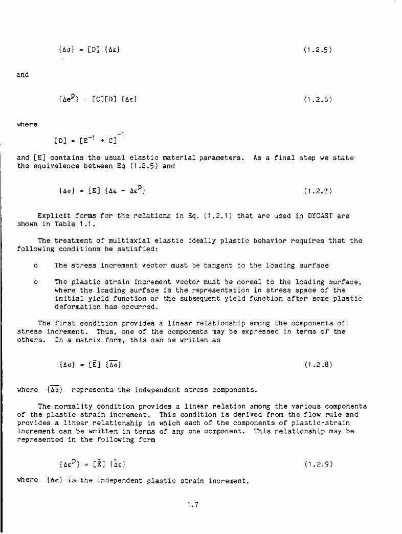
the equivalence between Eq (1.2.5) and

As a final step we state

{Ao} = [E] {A_ - Acp} (I .2.7)

Explicit forms for the relations in Eq. (1.2.1) that are used in DYCAST are

shown in Table 1.1.

The treatment of multiaxial elastic ideally plastic behavior requires that the

following conditions be satisfied:

o The stress increment vector must be tangent to the loading surface

The plastic strain increment vector must be normal to the loading surface,

where the loading surface is the representation in stress space of the

initial yield function or the subsequent yield function after some plastic

deformation has occurred.

The first condition provides a linear relationship among the components of

stress increment. Thus, one of the components may be expressed in terms of the

others. In a matrix form, this can be written as

(i.2.8)

where {Ae} represents the independent stress components.

The normality condition provides a linear relation among the various components

of the plastic strain increment. This condition is derived from the flow rule and

provides a linear relationship in which each of the components of plastic-strain

increment can be written in terms of any one component. This relationship may be

represented in the following form

{a_p} = [El {Zc}

where {_e} is the independent plastic strain increment.

(I .2.9)

1.7

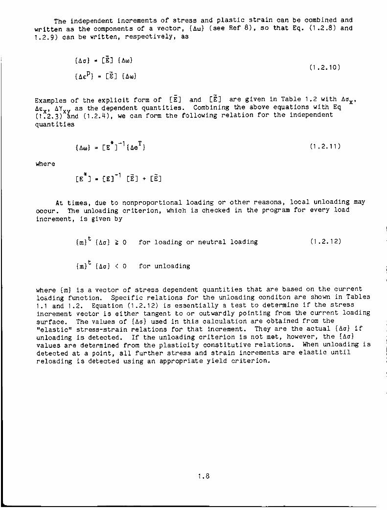
The independent increments of stress and plastic strain can be combined and

written as the components of a vector, {Am} (see Ref 8), so that Eq. (1.2.8) and

1.2.9) can be written, respectively, as

(I .2.10)

Examples of the explicit form of [E] and [E] are given in Table 1.2 with Ao x,

ACx, AYxy as the dependent quantities. Combining the above equations with Eq(1.2.3) and (1.2.4), we can form the following relation for the independent

quantities

where

* -I{Am} = [E ] {Ae T} (1.2.11)

* -I[E ] : [E] [E] + [_.]

At times, due to nonproportional loading or other reasons, local unloading may

occur. The unloading criterion, which is checked in the program for every load

increment, is given by

{m} t {Ae} _ 0 for loading or neutral loading (I .2.12)

{m} t {Ae} < 0 for unloading

where {m} is a vector of stress dependent quantities that are based on the current

loading function. Specific relations for the unloading conditon are shown in Tables

1.1 and 1.2. Equation (1.2.12) is essentially a test to determine if the stress

increment vector is either tangent to or outwardly pointing from the current loading

surface. The values of {A_} used in this calculation are obtained from the

"elastic" stress-strain relations for that increment. They are the actual {Aa} if

unloading is detected. If the unloading criterion is not met, however, the {Ae}

values are determined from the plasticity constitutive relations. When unloading is

detected at a point, all further stress and strain increments are elastic until

reloading is detected using an appropriate yield criterion.

1.8

TABLE 1.1 _C] Matrix for Various Stress States

PLANE STRESS - ISOTROPIC

'_ '_"tr_cI "l" ;." _;y

fCl_r2"l. _ 21 "_';Y'_;_-|m3m I m3m2 m3| m3 - 3_xy

D = _ ¢o_ , o o " yield stress , _,j - oCj - q£j

-2 -2 - - -2 2yield function: f " _x + 0y - OxOy + 3_xy " oo " 0

unloadtn 8 cr¢¢erton: mldo x + m2dCy + m3d_xy < 0

PLANE STRESS - ORTHOTROPIC

(cJ-_ 1.1.2 m_I 2-

I mlm3 m2m3 m3

"1" 2(G+H);x " 2HoY

m 2 - 2(F+H)Oy - 2Ho x

m 3 - z+S_xy

m 4 - -2FOy - 2Go x

D " c(m ÷ m_ + ÷ m&) , °tJ " °lj " olJ

yield func clon: f - (G+H) + (F+H) - 2H_x_y + 2.T2xy 1

unloading cr£cer£on: mldO x + m2doy + m3d_xy < 0

G+H = I/X2, H+G = I/Y 2, F+G = I/Z 2, 2N = I/T 2

X,Y,Z are yield stresses in tension in principal directions, T is yield stress in

shear in principal directions

ONE NORMAL STRESS - TWO SHEAR COMPONENTS

I m_ symmetric

|m3ml m3m2 # m3

m I " 0x

=2 " 3Txy

m 3 - 3Txz

D. + .20 , Oo- yi.:+.r., , :lj- otj- +i+

yi, id _..._o°. _. ;2+ 3:2÷ ::2=. °2°.ox xy z

unloadin g criterla: mldOx + m2d_xy ÷ m3d_xz < 0

1.9

TABLE 1.2 [I_]and [E] Matrices for Various Stress States

[_] -

PLANE STRESS - ISOTROPIC

I! "ml -m 2

I 0

0 II[Z] = mI 0

m 2 0

mI " (_y - ½ox)/(% - ½Oy)

m2 = 3Txy/ (a x - ½ay)

PLANE STRESS - ORTHOTROPIC

oi12 110 I , iE] = m I

0 0 m 2

m "((_">o,-"°x)/I<'÷")o.""o,)

" // - HOy)m 2 2L_xy ((F+H) c x

o!r0

0

G+H = I/X2, H+F = 1/Y 2, F+G = I/Z2, 2N = 1/T 2

X,Y,Z are yield stresses in tension in principal directions, T is yield stress in

shear in principal directions.

ONE NORMAL STRESS - TWO SHEAR COMPONENTS

[Zl -I!i-m 2

1

0

m1 = 3_xy/C x

[El - m I 0

m 2 0

m2 - 3Xyz/_ x

1.10

I .3 DYCAST FORMULATION - DEVELOPMENT OF EQUATIONS OF MOTION

The approach implemented in DYCAST is the updated Lagrangian formulation (Ref

16 - 18) for geometric nonlinearity. The derivation of the governing equations

based on this approach follows that originally presented in Ref 16 and 17 for static

analysis. The essentials of this method are that the solution is obtained

incrementally, starting from a reference state, CR, defined at time t for which the

states of stress, strain, and deformation are known. The next state, Cc, termed the

current state at time t + At is assumed to be incrementally adjacent to CR. Theproblem then reduces to solving for the incremental quantities, {Au} {As}, {Ae}

which are the increments in displacement, stress and strain in going from C R to

Cc. These quantities are all referenced to CR so that {As} and {AE} represent the

second Piola Kirchoff stress and Green's strain tensor respectively.

Once these quantities are obtained the coordinates of all points are updated by

{x} = {x} + {au} (I.3.1)

where {X} is the coordinate location in CR and the stress measure is transformed to

C c so that Cc is now the reference state for the next increment.

Based on these concepts, the equations of motion can be developed using he

principle of virtual work. If D'Alembert forces are treated as body forces, we canwrite

t .... t

[s+ns} _{_}dv + [ p{u+Au} _{nu}dv

VR VR

t

-- f {T + AT} 6{Au} ds (I .3.2)

S R

where p is the mass density, {S} and {T} are stresses and surface tractions referred

to CR, and {u} is the acceleration at time t in configuration, CR. The

incremental quantities {AE}, {As}, {Au}, and {u} are unknowns obtained in going

from CR to Cc. The dot notation refers to differentiation with respect to time.

The strain increment can be separated into a linear and nonlinear component,

{AE} = {Ae} + {An} (1.3.3.)

where each component of the vector can be written as

I .11

I (Aui ' + AUj, ilAeij : _ j

I (I .3.4)Anij : _ Aui,j Auj,i

Substituting Eq (I .3,3, 1.2.7) into Eq (I .3.2) and neglecting terms that arecubic and quadratic in the displacement increment yields the following functional

t .. t tf {Ae-Acp} [E]6{Ae}dv + f p{Au} _{Au}dv + f {S} 6{An} dvVR VR VR

{r} +

SR

t

{AT} 6 {Au} ds (I .3.5)

where the residual load vector is

t t

{r} = f {T} 6{Au}ds -f {S} 6{Ae}dv

SR V R

.. t

p{u} _{Au}dv (I .3.6)

and represents the equations of motion in configuration CR. In principle {r} should

be identically equal to zero. However, as will be seen, as a result of iinearizing

Eq (I .3.5), {r} in practice will not be zero. Its approximation, i.e., that {r} is

less than some prescribed error bound, will serve as a basis for an iterative

procedure used to satisfy the equations of motion. Equation (I .3.5) is used to

develop the matrix equations of motion once the finite element assumptions are made

for the displacement field in terms of nodal variables. Writing these symbolically

in matrix form as

{Au} --[N(x)] {Au(t)} (I .3,7)

for each element, substituting into Eq (1.3.5) and performing the appropriate

variation of displacement increments yields

I.12

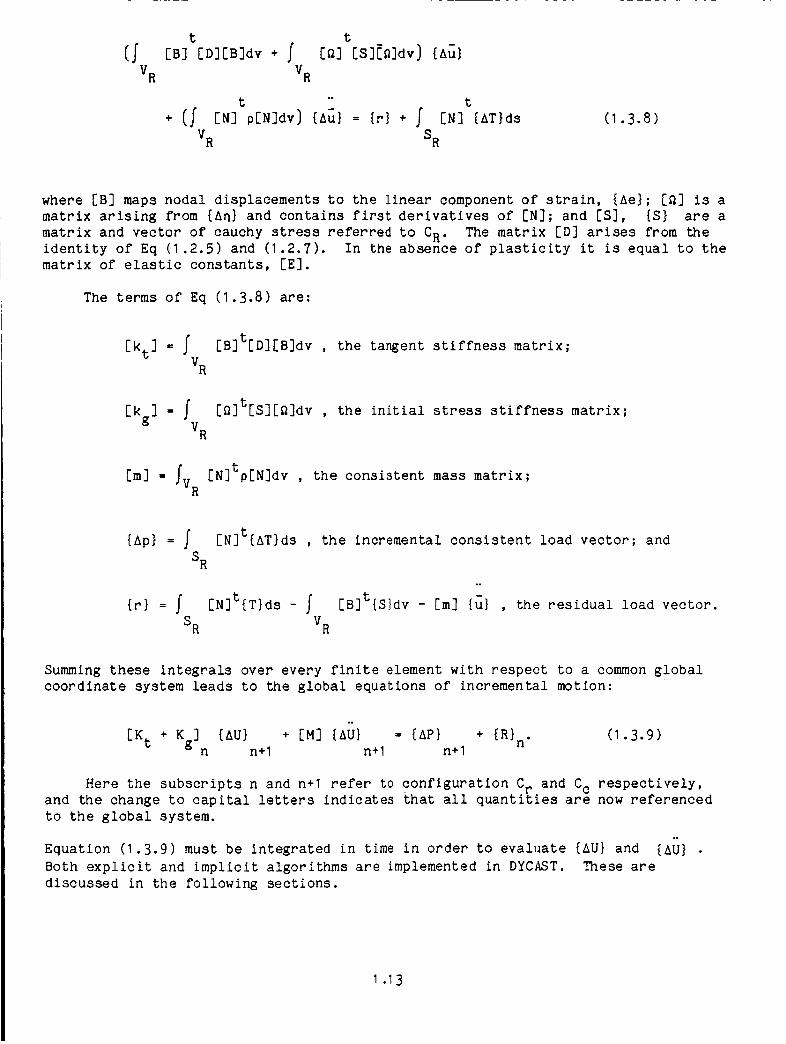
t t(Z [B] [D][B]dv + I [Q] [S][_]dv] {A_}

VR VR

t "° t

+ (f [N] p[N]dv) {Au} -- {r} + f [N] {AT}ds

V R SR

(I.3.8)

where [B] maps nodal displacements to the linear component of strain, {Ae}; [_] is a

matrix arising from {An} and contains first derivatives of IN]; and IS], {S} are a

matrix and vector of cauchy stress referred to CR. The matrix [D] arises from the

identity of Eq (1.2.5) and (1.2.7). In the absence of plasticity it is equal to the

matrix of elastic constants, [E].

The terms of Eq (1.3.8) are:

[k t] -- f [B]t[D][B]dv , the tangent stiffness matrix;

VR

[kg] = f [_]t[s][_]dv , the initial stress stiffness matrix;

V R

f [N]tp[N]dv , the consistent mass matrix;[m]- VR

{Ap} = f

SR

[N]t{gT}ds , the incremental consistent load vector; and

{r} = f [N]t{T}ds- f

SR VR

°.

[B]t{S}dv - [m] {u} , the residual load vector.

Summing these integrals over every finite element with respect to a common global

coordinate system leads to the global equations of incremental motion:

°.

[K t + Kg] {AU} + [M] {AU} -- {AP} + {R} n. (1.3.9)n n+1 n+1 n+1

Here the subscripts n and n+1 refer to configuration Cr and Cc respectively,

and the change to capital letters indicates that all quantities are now referenced

to the global system.

,.

Equation (1.3.9) must be integrated in time in order to evaluate {AU} and {AU}

Both explicit and implicit algorithms are implemented in DYCAST. These are

discussed in the following sections.

1 .13

1.4 DISCRETETIMEINTEGRATION

Muchattention has been given to methods for obtaining solutions to Eq(1.3.9). References 19 - 22 discuss methods for nonlinear dynamic analysis. Thestarting point for these is the choice of an appropriate schemeto integrate Eq(1.3.9) in time. Various methods for both linear and nonlinear structural analysishave been surveyed in Ref 23 and 24. Wewill not attempt to repeat the survey ofthese procedures here, but rather makesome general commentson the integrators usedin DYCAST. "

Onemeasureused to evaluate a time integrator is the size of the allowabletime step that can be used to yield accurate solutions. At the outset we state thata significant factor affecting time step size for a nonlinear dynamic analysis isthe degree of nonlinearity active in the analysis. That is, the time step must besmall enough so that the assumptions intrinsic to the governing equations, i.e.,plasticity theory and geometric nonlinearity, must not be violated. Because thenonlinearities mayvary during an analysis, it is our view that an integratorimplemented in a general purpose code for nonlinear dynamic analysis should be avariable time step procedure.

A variable time step procedure is one that enables the time step to be changedat different instants of the response, generally subject to stability and accuracyrequirements. Such a procedure has obvious advantages over one with a constant timestep, particularly in complex problems arising in practical applications because thesystem nonlinearities and dynamic response are varying continuously throughout theresponse history. This is particularly true for problems typical in crashsimulation. Basedon these commentsvariable time step integrators have beenimplemented in DYCAST. These are an explicit Modified Adamsintegrator (Ref 25),and the implicit Newmark-b (Ref 26) and Wilson-r (Ref 27) methods. Also implementedis a constant time step central difference explicit integrator (Ref 23).

The Choice of which of these methods to use is clearer for linear problems thanfor nonlinear ones, with implicit methods overwhelmingly used for gross structuraldynamics and explicit methods for problems where high frequency response issignificant, as in the treatment of wave propagation effects. Explicit integratorsare generally conditionally stable with the critical time step inverselyproportional to the highest frequency in the discrete model. Implicit integratorsare generally unconditionally stable for linear problems and tend to filter out thehigher frequency response. This allows for larger time steps, the choice of whichis controlled by the modesnecessary to predict the essential features of theresponse. The "best" implicit method is one that can filter the unwanted higherfrequency response without substantially altering the response in the lowerfrequency range of interest.

For linear problems using a constant time step, both methods lead tocoefficient matrices that are constant through the entire response spectrum. Thecomplicating factor for nonlinear problems is a consequenceof the change instiffness due to plasticity and geometric nonlinearities. In this case the explicitmethod leads to a constant coefficient matrix, but the implicit method mayrequirethe frequent reformulation of the coefficient matrix. The choice of which method touse in this case involves tradeoffs between a greater quantity of smaller less

I .14

costly time steps for explicit integration versus a lesser quantity of larger butrelatively more costly time steps for implicit integration. Reference to the term"costly" here is related to the degree of complexity and magnitude of subsidiarycomputations during each time step.

1.15

I .5 EXPLICIT INTEGRATION

It is convenient to recast Eq (I .3.9) into the following form when implementingan explicit time integration method•

where

°.

[M]{AU}n+ I -- {AP}n+ I + {R} n + {Af}n+ I (1.5•I)

{Af}n+ I = [K t + Kg] {AU}n+ I

is a vector of incremental internal forces. The implication here is that these

operations are performed on the element level rather than on the assembled arrays•

Alternatively (Ref 23), {Af}n+ I can be obtained directly from the corresponding

integral quantities in Eq (I •3.9). An expression for this vector is obtained

directly from previously calculated variables by making use of the discrete time

integrator so that the solution reduces to calculating a right hand side to Eq

°°

(I .5.1) and then solving for {AU}n+ I The term {R} n in Eq (I .5.1) represents an

imbalance force that arises due to the linearization of the equations of motion in

the n th step. It is carried forward as a correction to the n+Ith step.

The widely used constant step central difference technique has been implemented

in DYCAST. However, our preference is to use a variable time step (Ref 25),

Modified Adams - Predictor - Corrector method. This integrator automatically varies

the time Step to reflect current system stiffness and dynamic response. Our

experience with this method has been that it chooses time steps near those requiredby the central difference method.

The Modified Adams procedure is based on substituting a predictor solution for

{AU}n+ I into Eq (1.5.1)

{AU}Pnrl d -- {AU} dev + At {U} n +Ate_ {Un - Un-1} (1.5.2)

Equation (I.5.2) is the Taylor series expansion for {U}n+ I with the backwards

difference used for the acceleration and {AU} dev is the difference between the n thn

predictor and corrector solutions, {UC°rn - uPred}n Once {AU}n+ I is obtained

from Eq (I .5.1), the corrector solution is generated based on a forward difference

for the third term in Eq (I .5.2)

I .16

{u} _- " At " _ Un }Cor {U}n + At{U}n + 2-- {Un+ In+1

(I.5.3)

• .° ,°

U) COr {U} + At{U} + At _ Un }{ "n+1 -- n n _- [Un+1

An error criterion is used to ensure that the difference between the predictor and

corrector solutions satisfies some prescribed error value• In practice, the

convergence criterion usually fails on the difference between the predictor and

corrector velocities. This is

u,Cor u, Pred At { "" _ AUn}_n+1 - { _n+1 = 2- AUn+I(I•5•4)

and the error criterion is defined using a velocity error ratio, as

°. °°

< At AUn+1 - AUn < ¢. (1.5.5)2

Un+1

Whenever the error ratio is larger than the upper limit, the time step is halved.

Conversely, the time step is doubled whenever the error ratio is smaller than the

lower bound. It can be seen from Eq (1.5.5) that the error criterion limits the

rate of change of acceleration.

In that sense, the time step control is based solely on system dynamics• The

nonlinearities affect the time step only insofar as they affect system dynamics•

Thus, the explicit algorithm in DYCAST depends on the small time steps necessary

when using an explicit integrator to enforce the system nonlinearities.

Because of the ease in obtaining solutions to Eq (I•5.1), the computation time

for an explicit method becomes strongly dependent on the element level stress-strain

recovery and the formation of Af. Computer costs are therefore directly tied to the

number of elements in the discrete model and the number of time steps necessary in

the analysis. This leads to the major drawback of explicit methods, namely, that

more refined models have an increased frequency spectrum, requiring, for numerical

stability, a smaller time step. Consequently, there is a complementary effect

caused by a larger set of elements in combination with smaller time steps. Because

of this situation a break-even point occurs when the economics of simpler

calculations are overridden by the requirement of an increasing quantity of ever

smaller time steps•

1.17

1.6 IMPLICIT INTEGRATION

A variable time step implicit solution algorithm, based on the Newmark-Bfamilyof integrators is implemented in DYCAST. The recurrence relations for this methodare

"" I{u} =

n+1 BAt 21 {U}n I _{AU}n+ I - _-_ - (_-_ I){U} n

(I .6.1)

{AU}n+ I = At{U} n + YAt {AU}n+ I

The parameters B and Y affect the integration accuracy and stabilit X. Forlinear problems it can be shown that when Y _ 0.5 and B _ 0.25 (0.5 + Y) _ the

integrator is unconditionally stable. The case for which Y = 0.5, B = 0.25

represents the constant average acceleration method originally proposed by Newmark.

Substituting Eq (I .6.1) into Eq (I .3.9) yields

[Kin {AU}n+I = {AP}n+I + {Qd}n+1 + [R}n (I .6.2)

where

[K] n = [K t + Kg

M

8At 2

• .°

Un Un{Qd}n+ I = [M] {-_-_ + _-_}

Equation (1.6.2) is solved in two ways in DYCAST. The first is a simple

incremental method with a one-step equilibrium correction where

[K]n' {AP}n+I' {Qd}n+1 and {R} n are formed at the beginning of the step. The

unknown {AU}n+ I is then calculated from Eq (1.6.2). The vector {R} n is the

imbalance force from the previous step and prevents drifting from the true solution

due to the linearization of Eq (1.3.9).

This procedure is effective as long as the nonlinearities are not large in the

current step. Equation (I .3.9) can be solved iteratively at each time by requiring

that the equations of motion be satisfied to within some preset tolerance. In this

form Eq (I .6.2) becomes

1.18

[Kin {AU}_+I = {AP}n+I + {Qd}n+1 +iZ

j--o{R}J+I (I .6.3)

In this equation i signifies the iteration and

{R}j : {P - {F}j - [M] {'" Jn+1 }n+1 n+1 U}n+l (I .6.4)

where the terms are defined in Eq (1.3.6) and are, respectively, the vector ofexternal forces, the vector of internal forces, and the inertia forces, allevaluated at the end of the step.

Since {F} j is evaluated taking into account all system nonlinearities itn+1

serves as a feedback device to the linearized Eq (1.6.2). The coefficient matrix inthis procedure is formed only at the beginning of the step and held constant duringthe iterations. The solution algorithm is therefore classified as a Modified Newtonprocedure.

Whenj -- o, Eq (1.6.3) reduces to Eq (I .6.2) since

{R}°+1 -- {R}n

There are a number of ways to define convergence. DYCASTuses the followingcriterion:

• _ AU i-IAU_+I n+1

n+1

< _ (1.6.5)

m

where Un+1 = IUn+1 I max ' the maximum displacement within the model.

A variable time step procedure is defined by requiring that the number of

iterations in each time step be less than a prescribed value. If this criterion is

violated the time step is halved. Conversely if the solution converges in one

iteration for a prescribed number of steps the time step is increased by a factor of

1.5. An upper bound for the time step is user specified. The static analysis

procedure in DYCAST follows the same procedures as outlined above with the dynamic

terms suppressed.

1.19

1.7 DYCASTELEMENTLIBRARY

The basis for the derivation of the elements in DYCASTare in Ref I. Somedetails are also in Section 4.3 of this report. There are currently six elementtypes available for structural modelling, as described below.

Membrane Triangles - The membrane family of triangular elements implemented

includes

o three-node constant strain

o six-node linear strain

o four- and five-node transitional elements.

The terms constant, linear, and transitional refer to the strain distributions

that exist in the element as a consequence of choosing an assumed displacement

field.

Stringer Element - This element is used to represent a one-dimensional axialforce structural member. Two stringer elements are included: a two-node element

developed from a linear axial displacement field and a three-node element developed

from a quadratic axial displacement field.

Beam Element - There are two nodes with six degrees of freedom at each node,

three displacements, and three rotations. The element is based on a linear axial

displacement field and cubic transverse displacement. In the completely elastic

case, the beam stiffness matrix involves elastic material properties and integrated

quantities that depend on the cross section, the area and moments of inertia. Once

points on the beam are plastic, these integrals must be numerically evaluated. Some

details of the analysis are described below.

The beam linear strain component based on Kirchoff's hypothesis, neglecting

warping of a cross section and using linearized curvatures is

{Ae} = [Y] {Ax} (I .7.I)

where

[Y] :

E 0 z -yy 0

-z 0

A8 x ABy,xA8 }X 'X Z'X

I .20

and y, z, are coordinate locations in the cross section,

are the increments of axial strain, twist, and curvatures.

Making the assumptions for the displacement field,

AU, x A8 x ABy, A8 z'x x 'x

{_x} = [¢] {AU} (I .7.2)

where [¢] is based on a linear function for AU and ABx and a cubic for V and W.

The further assumption is made that the material stiffness properties in the

plastic state vary linearly in the axial coordinate,

[D] = [D]i (I - _) + [D]j (I .7.3)

where i,j denote quantities at the two nodes, _ = x/£ and x, £ are the axial

coordinate and length respectively. With these assumptions, the stiffness matrix

component, [kt], becomes

I

[kt] = £ f ([¢]t (I-{) f [Y]t[D]i[Y]dAo A

fo[Y]t[D]j [Y] dA ) [¢] dE

A

(I .7.4)

The area integrals in Eq (1.7.4) are evaluated numerically using Gauss-Legendre

integration. To accomplish this, the shape of the cross section must be known a

priori and the state of stress and strain must be evaluated at each integration

point in the cross section. Towards this end user-defined arbitrary cross-sections

and 12 pre-defined cross sections can be specified. These are shown in Table

4.3.1. An additional point to be made is that the torsional shearing stresses are

neglected in all the thin-walled open sections. However, because warping is

neglected in Eq (1.7.1) for the closed sections, the numerical integration can

overpredict the torsional stiffness. Because of this the terms in the second and

third row of [Y] are multiplied by a "knock down" factor

n= / JI + I (1.7.5)yy zz

where J is the user-specified torsional rigidity of the section and Iyy, Izz are thesection bending moments of inertia.

I.21

Nonlinear Sprin_ Element - A nonlinear spring element becomes an important

element in modelling a complex structure. It can be used

o to simulate structural sections for which the axial load versus elongation

behavior (or moment versus rotation) has been obtained either by a crush

test or by some other means

o to simulate an energy absorbing device

o as a gap element to approximate variable contact/rebound

o any combination of the above

The force versus elongation for this element is specified in tabular form. In

general, nonlinear spring elements dissipate energy by unloading stiffly from their

last deformation state along some specified unloading slope, thereby accumulating

non-recoverable permanent deformation. Upon reloading, the path is along the

unloading line to the previous maximum deformation state, at which point deformation

continues along the originally specified load versus deflection curve.

The undamped nonlinear spring element in principle can be used as a gap element

in order to simulate variable kinematic constraints that describe contact/rebound.

However, in practice, use of a gap element in a dynamic analysis leads to high

frequency oscillations because a large stiffness is associated with a small nodal

mass. To surmount this difficulty viscous damping must be introduced to the

nonlinear spring when used as a gap element. The damping coefficient is dependent

on the current stiffness so that before contact, i.e., zero stiffness, the damping

coefficient is zero. Spurious rebound can be further prevented by a "capture"

technique in which both the stiffness and damping parameter are maintained as long

as the contact point oscillates within a certain tolerance of the actual contact

position. This technique has been effective for a number of sample problems.

Plate Bending Element - A three-node triangular plate bending element has been

implemented in DYCAST. This element is based on the combination of the constant

strain triangle for in-plane behavior and an implied cubic variation for the

transverse deflection. The classical Kirchoff hypothesis, that plane sections

remain plane, is only forced in a discrete sense along the element edges as well as

the vertices. This results in a general plate bending element with three-

translational and three rotational degrees of freedom at each node.

Ground Contact Element - This element is used to simulate contact between a

node and a rigid plane. The perpendicular distance between the plane and the node

is monitored until contact is made. Once contact is made the element acts as a

nonlinear spring to enforce the contact condition.

I. 22

REFERENCES

I • A.B. Pifko, H.S. Levine, and H. Armen, Jr., "PLANS - A Finite Element Program

for Nonlinear Analysis of Structures, Volume I - Theoretical Manual," NASA CR-

2568 (1975)•

1 A. Pifko, H. Armen, Jr., A. Levy, and H. Levine, "PLANS - A Finite Element

Program for Nonlinear Analysis of Structures Volume II - User's Manual," NASA CR

145244 (1977)•

. R.G. Thomson and R.C. Goetz, "NASA/FAA General Aviation Crash Dynamics Program -

A Status Report," AIAA/ASME/ASCE/AHS 20th Structures, Structural Dynamics, and

Materials Conference," A Collection of Technical Papers on Design and Loads,

224-232 (1979).

4. R. Winter, A.B. Pifko, and H. Armen, "Crash Simulation of Skin-Frame Structure

Using a Finite Element Code," SAE Paper 770484 (1977).

. R. Hayduk, R.G. Thomson, G. Whittlin, and M.P. Kamat, "Nonlinear Structural

Crash Dynamic Analysis," SAE Paper 790588 (1979), SAE Business Aircraft Meeting,

Wichita, KS, (April 1979).

• R. Winter, A.B. Pifko, and J.D. Cronkhite, "Crash Simulation of Composite and

Aluminum Helicopter Fuselages Using a Finite Element Program," AIAA, J. of

Aircraft, Vol 17, No. 8, p 591 (August 1980).

. R. Winter, M. Mantus, and A.B. Pifko, "Finite Element Analysis of a Rear-Engine

Automobile," SAE Paper 811306 (1981), SAE Fourth International Conference on

Vehicle Structural Mechanics, Detroit, MI, (18-20 November 1981)•

t H.D. Carden and R.J. Hayduk, "Aircraft Subfloor Response to Crash Loadings," SAE

Paper 810614, SAE Business Aircraft Meeting, Wichita, KS (7-10 April 1981).

9. E. Alfaro-Bou, M.S. Williams, and E.L. Fasenella, "Determination of Crash Test

Pulses and Their Application to Aircraft Seat Analysis," SAE Paper 81061 I,

Business Aircraft Meeting, Wichita, KS (7-10 April 1981).

10. K.J. Saczalski and W.D. Pilkey, "Techniques for Predicting Vehicles Crash Impact

Response," Aircraft Crashworthiness, (edited by K. Saczalski, G.T. Singley III,

W.D. Pilkey, and R.L. Huston), Univ. Press of Virginia, Charlottesville, VA,

467-484 (1975).

11. K.J. Saczalski, "Modelling and Computational Solution Procedure of Prediction of

Structural Crash-Impact Response," Finite Element Analysis of Transient

Nonlinear Structural Behavior, (edited by T. Belytschko, J.R. Osias, and P.V.

Marcal), ASME, AMD-Vol 14, 99-118 (1975).

12. E. Alfaro-Bou, R.J. Hayduk, R.G. Thomson, and V.L. Vaughan, "Simulation of

Aircraft Crash and Its Validation," Aircraft Crashworthiness, (edited by K.

Saczalski, G.T. Singley III, W.D. Pilkey, and R.L. Huston), Univ. Press of

Virginia, Charlottesville, VA, 485-498 (1975).

I .23

13. R.S. Holmes, J.K. Gran, J.D. Colton, "Developing a NewVehicle Structure withScale Modeling Techniques," Measurementand Prediction of Structural andBiodynamic Crash-Impact Response, (edited by K.J. Saczalski and W.D. Pilkey),ASME,17-32 (1976).

14. H. Armen, "Plastic Analysis," Structural Mechanics Computer Programs, (edited by

W. Pilkey, K. Saczalski and H. Schaeffer), Univ. Press of Virginia,

Charlottesville, VA, 103-122 (1974).

15. H. Armen, Jr., A. Pifko, H. Levine, "Finite Element Analysis of Structures in

the Plastic Range, NASA CR-1649 (February 1971).

16. L.A. Hofmeister, G.A. Greenbaum, and D.A. Evensen, "Large Strain Elasto-Plastlc

Finite Element Analysis, AIAA J., _, 1248-1254 (1971).

17. H.S. Levine, H. Armen, R. Winter, and A] Pifko, "Nonlinear Behavior of Shells of

Revolution Under Cyclic Loading," J. Comput. Structures, _, 589-617 (1973).

18. K.J. Bathe, E. Ramm, and E.L. Wilson, "Finite Element Formulations for Large

Deformation Dynamic Analysis," Int. J. Num. Meth. Engineering, _, 353-386

(1975).

19. J.F. McNamara, "Solution Schemes for Problems of Nonlinear Structural Dynamics,"

J. Pressure Vessel Technology, ASME, 96, 96-102 (1974).

20. D.P. Mondkar and G.H. Powell, "Finite Element Analysis of Nonlinear Static and

Dynamic Response," Int. J. Num. Meth. Engineering, 11, 499-522 (1977).

21. J.A. Stricklin and W.E. Haisler, Comments on Nonlinear Transient Structural

Analysis, Finite Element analysis of Transient Nonlinear Structural Behavior,

(edited by T. Belytschko, J.R. Osias and P.V. Marcal), ASME, AMD-Vol 14, 157-178

(1975).

22. T. Belytschko and D.F. Schoebeule, "On the Unconditional Stability of a Implicit

Algorithm for Nonlinear Structural Dynamics," J. Appl. Mech., 97, 865-869

(1975).

23. T. Belytschko, "Transient Analysis," Structural Mechanics Computer Program,

(edited by W. Pilkey, K. Saczalski and H. Schaeffer), Univ. Press of Virginia,

Charlottesville, VA, 255-276 (1974).

24. J.R. Tillerson, "Selecting Solution Procedures for Nonlinear Structural

Dynamics," The Shock and Vibration Digest, 7, (1975).

25. H. Garnet and H. Armen, "A Variable Time Step Method for Determining Plastic

Stress Reflections from Boundaries," AIAA J., 13, 532-534 (1975).

26. N. Newmark, "A Method of Computation for Structural Dynamics," J. Eng. Mech.

Div., ASCE, 85, 67-94 (1959).

27. E.L. Wilson, L. Forhoomand, and K.J. Bathe, "Nonlinear Dynamic Analysis of

Complex Structures," Earthquake Eng. and Struct. Dyn., _, 241-252 (1973).

I.24

28. Hayduk, R.J., Winter, R., Pifko, A.B.; Fasanella, E.L., "Application of DYCAST-A Nonlinear Finite Element Computer Program - To Aircraft Crash Analysis";International Symposiumon Structural Crashworthiness, University of Liverpool,England, September 1983. In Structural Crashworthiness, Ed. by N. Jones and T.

Wierzlicki, Butterworth and Co., Boston 283-307, 1983.

29. Winter, R., Crouzet-Pascal, J., and Pifko, A.B., "Front Crash Analysis of A

Steel Frame Auto Using A Finite Element Computer Code" SAE paper 84-0728,

proceedings of the Fifth Internation Exposition on Vehicular Structural

Mechanics, SAE, April 1984.

30. Winter, R. and Pifko, A.B., "Finite Element Crash Analysis of Automobiles and

Helicopters," Proceedings of the International Conference on Structural Impact

and Crashworthiness, Imperial College, London, July 1984. In Structural Impact

and Crashworthlness, Vol 2, Ed. by J. Morton, Elselvier Applied Science

Publishers, New York, 278-309, 1984.

31. Crouzet-Pascal, J., Winter, R., and Gentzlinger, R., "Crash Resistance of C_-ved

Thin-Walled Beams", Recent Advances In En_ineerin_ Mechanics And Their Impact On

Civil Engineering Practice, Vol I, Ed_ by Chen, W.F. and Lewis, A.D.M., ASCE,

New York, 656-659, 1983.

I .25

This page intentionally blank

I .26

2.0 OVERVIEWOFPROGRAMINPUT

This section presents a general introduction to the card input for DYCAST. An80 character card image format is used.

The input begins with a title card that allows for any 80 character title(specified in columns 1-80). This title serves as a page heading for subsequentcomputer output. The input data following this card is divided into a number offunctional _roups, each describing a specific type of input information. These

groups are briefly described below and schematically shown in Fig. 2.3, (Page

2.6). Each input group must be read in the specific order listed below and shown in

Fig. 2. I. In each group, there are usually data subgroups that begin with a key

word. An index to all key words is in Table 2.3. The order of these key word

subgroups within the functional group can be varied. However, if the key word

subgroup contains more than one card, the sequence of those cards following the key

word is fixed. In general, each group is delineated with a section end card. This

is the alphanumeric SEND, left justified on the input card in columns I through 4.

After the initial title card the input groups are as follows:

Group A - Program Control Parameters and Options

Group B - Node Specification

This group defines an allowable set of node point identificationnumbers.

Group C - Element Connectivity

Defines each element by specifying its type, (i.e., beam, triangle ... ,

etc.) identification number, and connecting node points.

Group D - Node Point Coordinates

Defines the location of each node point in a global cartesian

coordinate system.

Group E - Node Point Single and Multipoint Constraints

Defines boundary conditions, nodal constraint equations, applied

displacements, and applied accelerations.

Group F - Node Point Initial Conditions

Defines node point initial displacements and velocities. This

section may be omitted if all initial displacements and velocities

are zero.

2.1

Group G - Added Inertia

Defines node point structural or nonstructural concentrated masses and mass

moments of inertia. This group is omitted when there are no nonstructural

concentrated masses and a consistent mass representation is to be used.

Group H - Element Material and Section Properties

Section properties include element thickness, area, and moment of

inertia where applicable. Material properties include such

quantities as Young's modulus, Poisson's ratio, and quantities

defining the material nonlinearities such as yield stress,

hardening parameters, and failure strains.

Group I - Applied Load and Time Function

Defines the spatial and time distribution of Applied Loads, if any.

This group is omitted if there are no applied loads or applied

displacements.

The last card in the deck is an alphanumeric STOP or END left justified on an

input card in columns I through 4. STOP indicates that the job is complete and END

indicates another problem input file follows.

Some general rules were used in designing the input. These rules are:

o

o

o

o

o

Most data cards that specify a new item of data begin with a "key-word" of

up to five characters, left justified in their appropriate field. For

example, cards specifying element connectivity for membrane triangles

begin with TRIM and single point constraints begin with SPC. An index of

all the key words is in Table 2.3, P. 2.7.

With one exception (Group B), all groups of data cards (see Fig. 2.1) end

with a card containing the key word group delimiter, SEND (Section End).

A "$" in column I of an input card is used to specify a comment line.

That line is ignored in the operational input stream. This allows the

user to insert descriptive headings and notes, as well as temporarily

deleting a line while leaving it in place.

The data file ends with one of two key words. If END is used, another

problem data file follows. If STOP is used, as will probably be the case

for most problems, the job ends.

Generally, two formats for input are used, E15.0 for floating point input

(fields of 15) and I5 for integer or fixed point input (fields of 5). The

fixed point (integer) data must be right justified. The floating point

data can be written in several forms. For example 10.0 can be input as:

10.0 any place in the field, or 1.0 E÷01, 1.0 E+I,

1.0EI, or I0, where the entry is right justified in the field.

2.2

o

o

There are a number of places in the program where lists of applicable nodeor element numbers must be specified with a set of data. In these casesthe nodes or elements are specified by entering the appropriate numbers onthe input cards in fields of five. However, for this purpose the user canalso utilize a shorthand form of the input. That is, specifying m and -n

consecutively is the equivalent of the specification of nodes or elements

m, m+1, m+2, ...n and specifying m, -p, and -n consecutively is the

equivalent of the specification of nodes (elements) m, m+p,m+2p ...m+kp

where m+kp is the highest integer in the sequence less than or equal to n.

For example, the specification of nodes I through 100 is written as 1-100

and nodes, i, 3, 5, ... 99 as I - 2 - 99. This card input appears in

fields of 5 (I5 format). Any number of continuation cards may be used. A

blank I5 field ends the specification. If any such card ends in the last

field, a blank card must follow.

Each input card set is described in the following section by first stating

its key word and then, in tabular form, describing the

(a) FORTRAN format

(b) columns on the input card reserved for the data

(c) descriptive symbols or names of the data

(d) brief comments - reference is made here where necessary, to a

more in-depth discussion in Section 4.

Physical units must be consistent in the system used. For example, if

inches_ seconds, _nd ib are units for length, time, and force, thenIb sect/in, lb/in _, and in/sec _ must be the units for mass, stress, and

acceleration Units for several systems are shown in Table 2.1. The

generic units for each input are indicated in parenthesis in the text,

with (L) referring to length, (T) referring to time, (F) referring to

force, and (M) referring to mass.

Some input parameters have default values already stored in the program,

as noted in the text. If the entry is left blank, the default value will

be used; otherwise, the entered value is used. Unless otherwise stated,

the default values are zero.

In most data input groups, duplicate inputs are not accepted, so that the

last entry value for a particular parameter will replace any previous

value. The only exception is Group G, Added Inertia, in which the values

of inertia assigned to each node are added to any values input

previously. This accumulation feature is a convience to the user'.

Inertia can be subtracted by assigning a negative number. Inertia can

also be changed during the course of an analysis, at a restart.

2.3

Table 2.1. Consistent Sets of Units

Length

Displacement Time

(L) (T)

in see

ft sec

cm sec

m sec

mm sec

sec

Energy,

Force Moment Mass

(F_ML/T 2) (FL) (MmFT2/L)

lb lb in ib sec2/in

lb ib ft ib sec2/ft

dyne dyne cm gm

N N m kg

kg kg mm kg sec2/mm

N N mm N sec2/mm

Rotary

Inertia Acce_. Stre_s(ML =) (L/T =) (F/L =)

lb sec 2 in in/sec 2 ib/in 2

lb sec 2 ft ft/sec 2 ib/ft 2

gm cm 2 cm/sec 2 dyne/cm 2

kg m2 m/sec 2 N/m 2

kg sec 2 mm mm/sec 2 kg/_m 2

N sec 2 mm mm/sec 2 N/mm 2.

*=M Pa

2.4

TABLE2.2

INPUT ITEMS

Time functions:

ACELT + PTME + PTM2 + PTM3

Multipoint constraint equations:

APPL + MPC

Beam element loads :

BMLO

Beam and stringer element sections:

CSEC + HCIR + HREC + HSEC +

ISEC + LSEC + LSEG + MSTG + SCIR +

SREC + TSEC + TWD + ZSCR + ZSEC

Plate and membrane element material

properties:

MATI + MAT2 ÷ MAT3

Beam element material properties:

MBM

Contact element and nonlinear spring

properties:

PGRD + PSPR

Single point constraints:

SPC

Plate element loads:

SURF

Plate and membrane element thickness:

THIK

MAXIMUM QUANTITIES FOR INPUT DATA

MAXIMUM QUANTITY

36 tables, 50 points per table

200 dependent nodes, 500

coefficients

I00 sets

200 sets

20 sets

50 sets

60 tables, 20 points per table

200 different 6-digit NBND code

words

100 sets

100 sets

Note: I. "Table" means a function defined by pairs of numbers (for example;

force and displacement, load and time).

2. "Set" means input data followed by a list of applicable elements.

. There are no limits to the quantities of nodes or elements, except

those imposed by the user to maintain economy of computational

expense (CPU) and modelling labor.

2.5

STOPEND OF DATA

I

_Ap END

50.0

PI

FLIED LOAD DISTRIBUTION AND TIME HISTORY

M_BM SEND /'_/11.2 E+06 0.333 /

I GROUP H/ ELEMENT MATERIAL AND SECTION PROPERTIES

I 3.45 E_)4

GROUP GNODE POINT STRUCTURAL OR NON STRUCTURAL

. . CONCENTRATED MASS AND MASS MOMENT OF INERTIA

| IVEL -528.0

I GROUP FI NODE POINT INITIAL DISPLACEMENT AND VELOCITIES /

S_pC SEND101010

IGROUFE ! J/NODE POINT SINGLE AND MULTIPOINT CONSTRAINTS J I

G_RRoDuSENDx,o , , <')PD

NODE POINT COORDINATES

SEND

J SEAM 1 1 2 10

J GROUP C

ELEMENT CONNECTIVITY

I

A

UP S NODE SPECIFICATION J

SEND I,J DYNA 0 10 100 _ I

/ ,i;*°* DYCAST EXAMPLE PROBLEM °'*

PROBLEM TITLE CARD J !

I"i

,yI

J '

i

Innut Data Organization

• Ii ! ;! I

iI !

! i

_j

2.6

TABLE 2.3 INDEX TO KEY WORDS

WORD

ACEL

ACELT

ADAM

APPL

BAND

BEAM

BMLO

CDIF

CNMI

CONC

CONM

CSEC

DELE

DYNA

EIGN

END

EOFF

FAIL

GRAV

GRDS

GRDX

GRDY

GRDZ

HCIR

HREC

HSEC

IDSP

ISEC

IVEL

LSEC

LSEG

LUMP

MATI

MAT2

GROUP

E

I

A

E

A

G

I

A

H

F

H

F

H

H

A

H

H

USAGE

DOF for Applied Accelerations

Time History of Applied Accelerations

Modified Adams explicit time integrator

Applied displacements and rotations of nodes

Re-order node list to reduce bandwidth

Beam element connectivity

Distributed Loads on beam element

Central difference explicit time integrator

Concentrated mass and rotary inertia

Concentrated force and moment at a node

Consistent nondiagonal mass matrix

Section properties for C-section beam elements

Manually delete (fail) members

First two control cards

Free vibrations

End a problem input, another problem follows

Turns off input data echo

Automatic member failure

Gravity Loading

Contact Element ConnectivityX-Coordinate for a set of nodes

Y-Coordinate for a set of nodes

Z-Coordinate for a set of nodes

Section properties for hollow circle beam elements

Section properties for hollow rectangle beam elements

Section properties for hat section beam elements

Initial displacements and rotations

Section properties for I-Section beam elements

Initial velocities

Section properties for L-section beam elements

Section properties for thin rectangle beam elements

Lumped diagonal mass matrix

Isotropic material properties for plane stress elements

Orthotropic material properties for plane stress with

perfect plasticity

PAGE

3.47

3.108

3.5

3.47

3.24

3.27

3.99

3.6

3.55

3.98

3.11

3.74,76

3.10

3.111

3.21

3.20

3.107

3.28

3.34

3.35

3.36

3.74,77

3.74,78

3.74,79

3.50

3.74,80

3.52

3.74,81

3.74,82

3.12

3.59

3.61

2.7

TABLE 2.3 INDEX TO KEY WORDS (Continued)

WORD

MAT3

MBET

MBM

MPC

MPRIN

MSTG

MSTR

NEWM

NPRIN

PFTAB

PGRD

PITC

POFF

PSPR

PTME

PTM2

PTM3

REST

ROLL

SCAN

SCIR

SEND

SPC

SPNG

SREC

STAT

STOP

STRG

SURF

THIK

TIME

TRIM

TRP2

TSEC

TWD

GROUP

H

H

H

E

A

A

A

H

D

A

H

I

I

I

A

D

A

H

E

C

H

An

C

I

H

A

C

C

H

H

USAGE PAGE

Orthropic material properties for plane stress with 3.64

strain hardening

Angle between local element axes and principal directions 3.69

of orthotropy

Material properties for beam elements 3.72

Multipoint constraints 3.46

Print member solution data 3.15

Material and section properties for stringer elements 3.70

Print stress and strain details for beam elements 3.23

Newmark-Beta implicit time integrator

Print nodal solution data3.7

3.16

Print summary table of plastic and failed elements 3.19

Contact Element Properties 3.92

Y-Rotation of vehicle coordinate system 3.41

Turns off printout of processed input data 3.22

Properties for spring elements 3.90

Time function for all applied loads and displacements 3. 102

Time function for all loads at a node 3.103

Time function for a load component at a node 3. 105

Restart parameters

X-Rotation of vehicle coordinate system

Scan input for errors, no solution

Section properties for solid circle beam elements

Ends data for a group

Single point constraints

Spring element connectivity

Section properties for solid rectangle beam elements

Static analysis

End a problem input, last card

Stringer element connectivity

Distributed loads on plate elements

Thickness and layers for plate and membrane elements

Print breakdown of computer time

Triangular membrane element connectivity

Triangular plate element connectivity

Section properties for T-section beam elements

Section properties for beam element constrained to move

in one plane

3.17

3.42

3.14

3.74,84

3.44

3.29

3.74, 85

3.9

3.111

3.30

3. 100

3.68

3.13

3.31

3.32

3.74,86

3.74,87

2.8

TABLE2.3 INDEXTOKEYWORDS(Continued)

WORD

WLSN

XSHF

YAWYSHF

ZSCRZSECZSHF

GROUP

A

D

DD

HHD

USE

Wilson-Theta implicit time integrator

X-Shift of vehicle coordinate system.

Z-Rotation of vehicle coordinate system.Y-Shift of vehicle coordinate system.

Section properties for reversed Z-section beamelementsSection properties for Z-section beamelementsZ-shift of vehicle coordinate system.

PAGE

3.8

3.37

3.403.38

3.74,883.74,893.39

2.9

This page intentionally blank

2.10

3.0 INPUTPREPARATION

This section serves as a basic guide for preparing input data for DYCAST. Assuch, it is our intention to write a concise and easily followed set ofinstructions. To accomplish this goal the depth of someof the explanations islimited here. Further in-depth explanations are reserved for Section 4 which servesas a more detailed reference. Specific reference is madeto these sections asneeded.

3. I PROBLEMTITLE

/ Card I: Any 80 Character Title /

This 80-character title card serves as a heading for all pages of

output. Any number of continuation title cards can be specified. This is

indicated with three blanks and a comma in columns 77 through 80. The

continuation title cards only appear on the first page of the output.

Additional problem description can be included on any number of comment

cards following the title card. These comment cards begin with a "$" in

column I, and will appear only on the first page of the output.

NOTES:

I. This card must be the first one in the data file.

2. A "$" in column I of any card in the input stream indicates that it is a

comment card, to be ignored by the program.

3.1

3.2 GROUPA - PROGRAMCONTROLPARAMETERSANDOPTIONS

Only four cards in this group are required; two DYNAcards, a time integratorcard, and the SENDcard.

/ Key Word DYNA /

This required card must always follow the title card. (Section 4.1.1)

Format Columns Symbol Comments

A4 I-4 DYNA Key word

5,6 Blank

411 7-10 NPNTC Prints diagnostic data (p. 4.1). Enter a I

in Col. 7 to print load vector, I in Col 8

for element mass and stiffness matrices, I in

Col. 9 for coeff, matrix entries and their

stacking indices, I in Col. 10 for assembled

coeff, matrix. Default = 0000.

I5 11-15 NPRNT Results printed every NPRNT time steps,

(default is last time step, corresp, to

FTIME, p. 3.4 ). Note I.

I5 16-20 NFORM

21 -80

Coefficient matrix reformed every NFORM

time steps (see Section 4.1.1). Default =

99999. Note 2.

Blank

NOTES :

I • NPRNT controls the frequency of printout requested by the TIME, MPRIN,

NPRIN, PFTAB, and MSTR cards defined below.

• The coefficient matrix is the mass matrix for explicit time intgrators

(CDIF and ADAM) and is a combination of the mass and stiffness matrices

for implicit integrators (STAT, NEWM, and WLSN). NFORM is set to I

internally for implicit integration. For explicit, use the default.

3.2

/ Key Work DYNA/, continued from previous page

e The program is dimensioned for 1000 nodes and 1000 elements (MXNOD = 1000,

MXMEM _ 1000). The amount of core required is according to the following

relations:

NCORE J > 22 (MXNOD) + 9 (MXMEM), to process input

NCORE J > 10 (No. of DOF), to enter calculation phase

The program will use the more efficient in-core solution (stack the

coefficient matrix in one pass) if:

NCORE J > SN - .5S 2 + N + .5S + 2000

where S = Maximum semi-bandwidth, N = No. of DOF

3.3

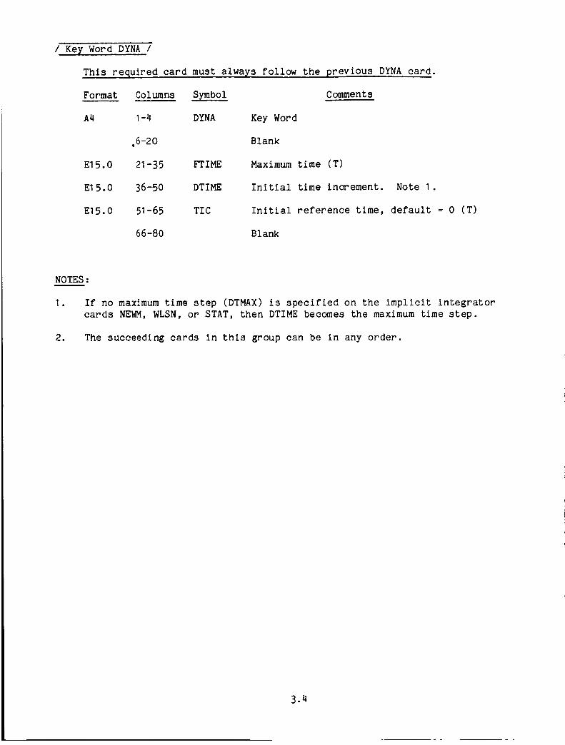
/ Key Word DYNA /

This required card must always follow the previous DYNA card.

Format Columns Symbol Comments

A4 I-4 DYNA

.6-20

E15.0 21-35

El 5.0 36-50

E15.0 51-65

66-80

FTIME

DTIME

TIC

Key Word

Blank

Maximum time (T)

Initial time increment. Note I.

Initial reference time, default _ 0 (T)

Blank

NOTES:

I. If no maximum time step (DTMAX) is specified on the implicit integrator

cards NEWM, WLSN, or STAT, then DTIME becomes the maximum time step.

2. The succeeding cards in this group can be in any order.

3.4

/ Key Word ADAM /

This card is specified qnly if the Modified Adams explicit time integrator

is to be used. (Sections 1.5 and 4.1.3)

Format Columns Symbol Comments

A4 I-4 ADAM

5

E15.0 6-20 EPSIL

El 5.0 21 -35 DELTA

El 5.0 36-50 ERR

51-80

Key word

Blank

Upper bound convergence error.

Default is .10 (10%)

Lower bound convergence error.

Default is .01 (1%)

Tolerance on convergence test.

Default is I. x 10-4 (Section 4.1.3)

Blank

NOTES:

I. One of the following key words must be input to specify the integrator or

type of solution: ADAM, CDIF, NEWM, WLSN, STAT, EIGN.

3.5

/ Key Word CDIF/

This card is specified only if the central difference explicit time

integrator is to be used.

Format Columns Symbol Comments

A4 I-4 CDIF Key word

5-80 Blank

NOTES :

I • One of the following key words must be input to specify the integrator or

type of solution: ADAM, CDIF, NEWM, WLSN, STAT, EIGN.

3.6

/ Key Word NEWM/

This card is specified only if the Newmark-BETA implicit time integrator

is used. (Section 1.6)

Format Columns Symbol

A4 I-4 NEWM Key word

Comments

5 Blank

El 5.0 6-20 BETA Parameter beta appearing in expres-

sion for displacement in Newmark -

Beta method (default is .25 if both

BETA and GAMA are blank). If GAMA is

non-zero and BETA is zero then

8 = (.5 + Y)2/4.

El 5.0 21 -35 GAMA Parameter gamma appearing in expres-

sion for velocity in Newmark-Beta

method (default is .5 if field is

blank).

El 5.0 36-50 TOL Limit on convergence test for itera-

tions within a time step. (Default is

.01 ) i.e.,

AU i - AU i-I< TOL

El 5.0 51 -65 INTER

El 5.0 66-80 DTMAX

where i -- iteration number

Maximum number of iterations per

time step (default is 10). If INTER

< 0 the iterations are suppressed

and a constant time step is used

Maximum allowable time step (default

is original DTIME from second DYNA card

p. 3.4) (T)

NOTES:

I . One of the following key words must be input to specify the integrator or

type of solution: ADAM, CDIF, NEWM, WLSN, STAT, EIGN.

o This procedure assumes a consistent mass matrix. If only lumped mass is

desired, set the density equal to zero on all material property cards in

Group H, and add the lumped mass to the nodes in Group G.

3.7

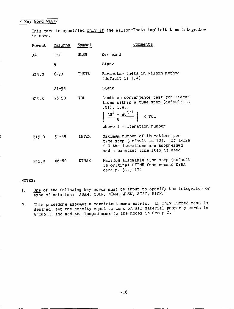
/ Key Word WLSN/

This card is specified only if the Wilson-Theta implicit time integrator

is used.

Format Columns Symbol

A4 I-4 WLSN Key word

Comments

Blank

E15.0 6-20 THETA Parameter theta in Wilson method

(default is 1.4)

21 -35 Blank

El 5.0 36-50 TOL Limit on convergence test for itera-

tions within a time step (default is

.01), i.e.,

I AU i - AU i-IU < TOL

where i -- iteration number

El 5.0 51 -65 INTER Maximum number of iterations per

time step (default is 10). If INTER

< 0 the iterations are suppressed

and a constant time step is used

El 5.0 66-80 DTMAX Maximum allowable time step (default

is original DTIME from second DYNA

card p. 3.4) (T)

NOTES :

I , One of the following key words must be input to specify the integrator or

type of solution: ADAM, CDIF, NEWM, WLSN, STAT, EIGN.

. This procedure assumes a consistent mass matrix. If only lumped mass is

desired, set the density equal to zero on all material property cards in

Group H, and add the lumped mass to the nodes in Group G.

3.8

/ Key Word STAT/

This card is specified only if a static analysis is to be used.(Section 4.1.5)

Format Columns Symbol

A4 I-4 STAT Key word

Comments

5-35 Blank

El 5.0 36-50 TOL Limit on convergence test for itera-

tions within a time step (default is

.O1) i.e.,

I AU i - AU i-I [I < TOLU

where i = iteration number

El 5.0 51 -65 INTER Maximum number of iterations per

time step (default is 10). If INTER

< 0 the iterations are suppressed

and a constant time step is used.

El 5.0 66-80 DTMAX Maximum allowable time step for

computations of load increment

(default is the original DTIME from the

second DYNA card, p. 3.4) (T)

NOTES:

I • One of the following key words must be input to specify the integrator or

type of solution: ADAM, CDIF, NEWM, WLSN, STAT, EIGN.

. Static loads and displacements are applied incrementally by calculating

the product of the load distribution factors (Group I) or displacement

factors (APPL, Group E) times the time function PTME in Group I. See

Section 4.6.

3.9

/ Key Word EIGN/

This card is specified only if a free _ibration analysis is desired.

(Section 4.1.6)

Format Columns Symbol

A4 I-4 EIGN Key word

Comments

5 Blank

E15.0 6-20 IQ Number of modes desired, up 100.

El 5.0 21-35 NSBAR Number of times reorthogonalization

is to be performed. Usually 2 is

sufficient

El 5.0 36-50 LP RINT If set equal to I the factoredstiffness matrix and mass matrix are

printed, otherwise zero or blank

El 5.0 51 -65 IPRINT If set equal to I intermediate

debugging information is printed

E15.0 66-80 EPS Shift parameter used when the

stiffness matrix is singular

(Section 4.1.6) Default = O.

NOTES :

I o One of the following key words must be input to specify the integrator or

type of solution: ADAM, CDIF, NEWM, WLSN, STAT, EIGN.

3.10

/ Key Word CONM/

This optional card specifies that the structural mass will be calculated

using a consistent mass approach. This is the program default condition.

Format Columns Symbol Comments

A4 I-4 CONM Key word

5-80 Blank

NOTES:

I. The nodal inertias specified in Group G form a diagonal matrix which is

added to this structural mass matrix.

3.11

/ Key Word LUMP/

This optional card specifies that all the mass properties of the structure

have been defined using concentrated (or lumped) masses and inertias.

This card denotes a diagonal mass matrix for explicit integration.

Format Columns Symbol Comments

A4 I-4 LUMP Key word

5-80 Blank

NOTES :

!. Default condition is consistent mass (CONM).

. Lumped masses are not internally calculated for the elements. They must

be input in Group G.

, Lumped (diagonal) mass matrices are not reformed, regardless of the NFORM

value specified on the first DYNA card, P. 3.2.

. This card will be ignored for implicit integrators (NEWM, WLSN). However,

a diagonal (lumped) mass matrix can be used with implicit integrators by

specifying the proper nodal masses in Group G and using zero material

densities in Group H (the latter to suppress the consistent structural

mass matrix).

3.12

/ Key Word TIME/

This optional card initiates printout every NPRNT steps (P. 3.2) of

computer time (CPU) used at various parts of the computation. (See

Section 4.1.2 for an example of this output)

Format Columns Symbol Comments

A4 I-4 TIME Key word

5-80 Blank

NOTES :

3.13

/ Key Word SCAN/

This optional card indicates that the input is to be read and processed

but operations will stop just before calculating and forming the stiffness

and mass matrices. This feature is used to check input data before a full

job execution is tried.

Format Columns Symbol Comments

A4 I-4 SCAN Key word

5-80 Blank

NOTES:

3.14

/Key Word MPRIN/

This optional set of at least two cards specifies the elements for which

stress, strain, and load information will be printed every NPRNT steps (p.

3.2). Default condition: If this card is not specified, printout will

occur for every element• In order to suppress all element printout use

the key word MPRIN followed by a blank card.

Card I:

Format Columns Symbol Comments

A5 I-5 MPRIN Key word

6-80 Blank

Card(s) 2:

The second and succeeding card(s) contain the elements to be printed as

indicated below.

Format Columns Symbol

1615 1-80 MEM

Comments

Elements for which data is to be

printed are specified in fields of 5

(I5 format). The short form

notation and also any number of

continuation cards may be used. A

blank I5 field ends the specifica-

tion of the elements to be printed.

NOTES:

I •

2.

•

If an element list ends in the last field, a blank card must follow.

For beam elements, the default condition is to print a short table for

each beam, deleting the stresses and strains through the cross-section.

If these beam stress & strain data are to be printed, the MSTR card (p.

3.23) must also be used.

On a restart, if this card set is not included, MPRIN defaults to the

input used on the initial segment.

3.15

/ Key Word NPRIN/

This optional set of at least two cards specifies the nodes at which

displacement, velocity and acceleration are to be printed every NPRNT

steps (p. 3.2). Default condition: If this card is not specified

printout will occur for every node. In order to suppress all node

printout use the NPRIN followed by a blank card.

Card I :

Format Col umns Symbol

A5 I-5 NP RIN Key word

Comments

6-80 Blank

Card(s) 2:

The succeeding card(s) after the NPRIN card contain the nodes to be

printed as indicated below.

the

Format Columns Symbol

16 I5 I-80 NODE

Comments

Nodes for which data are to be

printed are specified in fields of 5

(I5 format). The short form

notation and also any number of

continuation cards may be used. A

blank I5 field ends the specification of

nodes to be printed.

NOTES:

I. If a node list ends in the last field of a card, a blank card must follow.

2. On a restart, if this card set is omitted, NPRIN defaults to the input

used in the initial segment.

3.16

/ Key Word REST/

This optional card specifies information for creating an external data

base or "restart" file, which is required for post-processing or

restarting the analysis. (Section 4.1.4, p. 4.6)

Format Columns Symbol Comments

A4 I-4 REST Key word

5 Blank

El 5 .0 6-20 IREST = 0. No restart file written (default when

this card is omitted).

= I. Initiate a restart file, written on

unit 21.

= 2. Continue from existing restart

file. The old file remains unchanged on

unit 21. Old and new output data will be

written on a new file on unit 22, if

NUTAP > 0 below.

= 3. Continue from existing restart

file. New output data will be added to the

existing file on unit 21, if NUTAP > 0 below.

El 5.0 21 -35 NUTAP When IREST = 0. or I., NUTAP is ignored.

When IREST = 2. or 3., set NUTAP = O. for no

new restart file, or NUTAP = I. to create new

restart file.

El 5.0 36 -50 IPRNT Restart data written every IPRNT time steps

to allow restart in a later continuation

run. If equal to zero, restart data are

written only at the final time. Note 2.

El 5.0 51 -65 NRSRT This number defines the starting time for the

continuation job from a restart file. It is

one of a set of NRSRT numbers, each

associated with a specific time, that are

printed out in the job that generated the

restart file. Restart segments can begin at

any time for which an NRSRT number has been

specified.

66-80 Blank

NOTES :

I. Only title card and Group A input data are required with a restart.

.

3.

IPRNT should be chosen to be as large as possible to reduce I/O and

storage requirements.

Group G data can also be specified with a restart (i.e. added inertia).

3.17

/ Key Word DELE/

This optional set of at least two cards specifies elements to be failed

manually. This card is optional and only has meaning when a problem is

beln_ restarted. (Section 4.1.9)

Card I:

Format

A4

e

Columns Symbol Comments

I-4 DELE Key word

5-80 Blank

Card(s) 2:

The second and succeeding card(s) contain the elements to be deleted.

Format Columns Symbol

16 I5 I-80 MEM

Comments

Elements to be deleted are specified

in fields of 5 (I5 format). A blank

I5 field ends the specification of

the deleted members. (The short form

input notation is not permitted here.)

NOTES:

I • If an element list ends the last field of a card, a blank card mustfollow.

. A deleted element cannot be subsequently restored. Therefore it is

necessary to specify its number here only once. However, it will be

convenient to leave the previously specified elements on the card, and add

new ones as desired, at each subsequent restart.

. The mass of a deleted element remains at its nodes. Nodes completely

detached from the rest of the structure become separate bodies.

. Mass can be added or subtracted in Group G at any node on a restart. Mass

can be completely deleted on a restart by subtracting its entire value.

3.18

/ Key Word PFTAB/

If this optional card is input a table is printed every NPRNT steps

(p. 3.2), indicating the elements that have been plastic, failed, or

deleted.

Format

A5

NOTES :

(Sectlon 4.1.8)

Columns Symbol Comments

I-5 PFTAB Key word

6-80 Blank

3.19

/ Key Word FAIL/

If this optional card is used, the stiffness and stress at each

integration point of an element will be deleted when its specified failure

criterion has been satisfied. The failure criteria are specified along

with other material properties in Group H. If no failure criteria are

specified for an element, its failure will not be evaluated. If this card

is omitted, no deletion action will be taken, but a warning message will

be printed when complete failure of an element would have occurred. See

p. 4.10.

Format Columns Symbol Comments

A4 I-4 FAIL Key word

5-80 Blank

NOTES:

I. Element continues to carry load if the FAIL card is not specified.

3.20

/Key Word EOFF/

This optional card will delete the printout (echo) of the user's input

data stream, except that the Group A data (Controls) echo will still be

printed.

Format Columns Symbol Comments

A4 I-4 EOFF Key Word

5-80 Blank

Notes:

3.21

/Key Word POFF/

This optional card will delete the printout of the processed input data

that follows the echo of input data, except that the processed Group A data

(controls) will still be printed.

Format Columns Symbol Comments

A4 I-4 POFF Key word

5-80 Blank

Notes:

3.22

/ Key Word MSTR/

If this optional card is specified, stress and strain output will be

printed for each integration point in the cross section at both ends of

beam elements for which printout has been requested by the MPRIN card set.

(p. 3.15)

Format Columns Symbol

A4 I-4 MSTR

5-8O

Key word

Blank

Comments

NOTES:

I. If this card is used, the beam printout will be one beam element per page,

compared to four per page without this card.

3.23

/ Key Word BAND/

This optional card causes the program to re-order the Group B node list to

produce a reduced bandwidth of the coefficient matrix, in order to reduce

the core storage requirements and the computer processing time. After

finding the optimum (or near-optimum) nodal order for minimizing the

bandwidth, the program will use this re-ordered node list as the Group B

input and proceed with the problem calculations. The re-ordered Group B

input is also written as an output file on unit 7 in the proper format for

direct use as input for subsequent problems.

Format Columns Symbol Comments

A4 I-4 BAND Key word

5 Blank

El 5.0 6-20 JMAX Maximum number of nodes

connected to any one node.

Default = 12.

21-80 Blank

NOTES:

I • For large problems, this card is essential to reduce computer resource

utilization.

2. MPC connectivities are automatically included•

. This BAND operation also works with SCAN (p. 3.14) as a pre-processor for

re-ordering the node list, without proceeding with the solution•

, The re-ordered node list from unit 7 should be used as input for Group B,

p. 3.24, and the BAND card should be deleted for subsequent runs to save

CPU time.

3.24

/ Key Word SEND/

This required card ends Group A data.

Format Columns

A4

Symbol

I-4 SEND Key word

5-80 Blank

Comments

NOTES :

I .

.

If this is a restart job only Group A input is required. In this case,

this SEND card is followed by a STOP or END card, p. 3.111.

Mass can be changed on a restart run by adding Group G data immediately

following Group A, then a final STOP or END card, p. 3.111.

3.25

3.3 GROUPB - NODESPECIFICATION

This required input group defines the allowable set of node numbers.Every node specified in the subsequent input groups must be listed here.While the node numberscan be in any order, they are converted within theprogram to consecutive internal numbers. Any quantity of cards maybeused. SeeNote 2 below and Section 4.2.

/Key Word

Format

1615

No Key Word for this Group /

Columns Symbol Comments

I-80 NODE The list of node numbers in fields of 5 (I5

format). The short form notation (p. 2.3)

and blank fields are allowed• Note I.

NOTES :

I • If the list ends in the last field of any card, a blank card must follow

to end this group.

1 This nodal sequence should be optimized in large problems to produce

minimum semi-bandwidth. This can be done using the SATELLITE

preprocessing program (Section 5.1) or the BAND card, p. 3.24.

3. A SEND card must not be used to end this group.

3.26

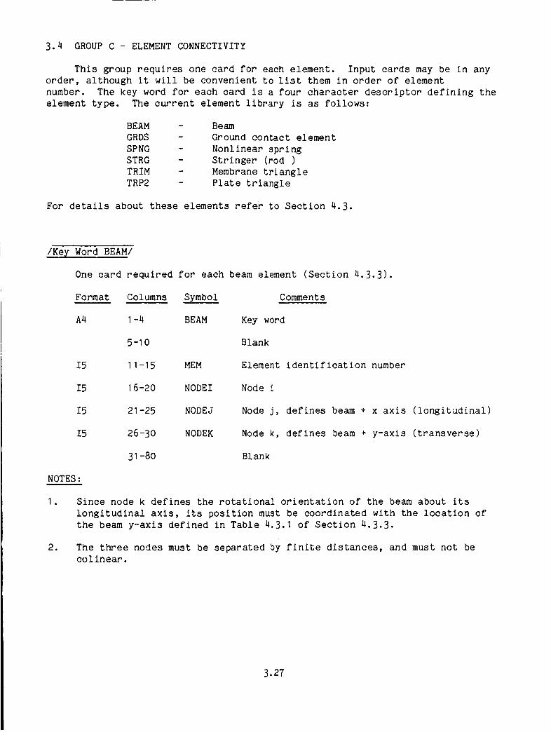
3.4 GROUPC - ELEMENTCONNECTIVITY

This group requires one card for each element. Input cards may be in anyorder, although it will be convenient to list them in order of elementnumber. The key word for each card is a four character descriptor defining theelement type. The current element library is as follows:

BEAMGRDSSPNGSTRGTRIMTRP2

BeamGround contact elementNonlinear springStringer (rod)MembranetrianglePlate triangle

For details about these elements refer to Section 4.3.

/Key Word BEAM/

One card required for each beam element (Section 4.3.3).

Format Columns Symbol

NOTES :

I •

•

A4 I-4 BEAM

5-I0

I5 11-15 MEM

I5 16-20 NODEI

I5 21-25 NODEJ

I5 26-30 NODEK

31-80

Comments

Key word

Blank

Element identification number

Node i

Node j, defines beam + x axis (longitudinal)

Node k, defines beam + y-axis (transverse)

Blank

Since node k defines the rotational orientation of the beam about its

longitudinal axis, its position must be coordinated with the location of

the beam y-axis defined in Table 4.3.1 of Section 4.3.3.

The three nodes must be separated by finite distances, and must not be

colinear.

3.27

/Key Word GRDS/

One card required for each ground contact element (Section 4.3.7).

Format Columns

A4 I-4

5-I0

I5 11-15

I5 16-20

I5 21 -25

26-80

Symbol

GRDS

MEM

NODE

NDIR

Comments

Key Word

Blank

Member identification number

Contact node

Global direction closest to the normal to the

contact plane,

I _ x

2 =y

3 =z

Blank

NOTES :

3.28

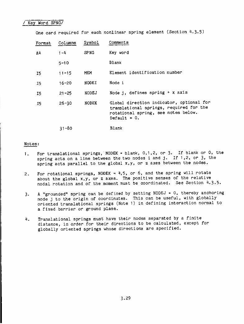
/ Key Word SPNG/

One card required for each nonlinear spring element (Section 4.3.5)

Format Columns Symbol

A4 I-4 SPNG

5-10

I5 11-15 MEM

I5 16-20 NODEI

I5 21-25 NODEJ

I5 26-30 NODEK

31-80

Comments

Key word

Blank

Element identification number

Node i

Node J, defines spring + x axis

Global direction indicator, optional for

translational springs, required for the

rotational spring, see notes below.

Default _ O.

Blank

Notes:

I • For translational springs, NODEK _ blank, 0,1,2, or 3. If blank or O, the

spring acts on a line between the two nodes i and j. If 1,2, or 3, the

spring acts parallel to the global x,y, or z axes between the nodes.

.

.

For rotational springs, NODEK = 4,5, or 6, and the spring will rotate

about the global x,y, or z axes. The positive senses of the relative

nodal rotation and of the moment must be coordinated. See Section 4.3.5.

A "grounded" spring can be defined by setting NODEJ = O, thereby anchoring

node j to the origin of coordinates. This can be useful, with globally

oriented translational springs (Note I) in defining interaction normal to

a fixed barrier or ground plane.

. Translational springs must have their nodes separated by a finite

distance, in order for their directions to be calculated, except for

globally oriented springs whose directions are specified.

3.29

/Key Word STRG/

One card required for each stringer element (Section 4.3.2).

Note:

I.

Format Columns Symbol Comments

A4 I-4 STRG Key word

5-10 Blank

I5 11-15 MEM Element identification number

I5 16-20 NODEI Node i

I5 21-25 NODEJ Node j, defines + x axis

I5 26-30 NODEK Node k, mid-length node, optional.

Default = O.

31-80 Blank

.

The mid-length node is provided to allow compatibility with the mid-side

node of an adjacent TRIM element

The nodes must be separated by a finite distance.

3.30

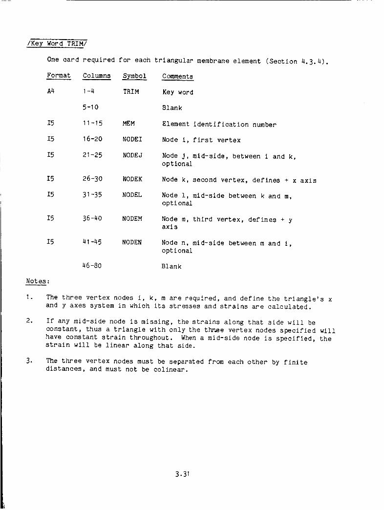
/Key Word TRIM/

One card required for each triangular membrane element (Section 4.3.4).

Format Columns Symbol

A4 I-4 TRIM

5-I0

I5 11 -1 5 MEM

I5 16-20 NODEI

I5 21 -25 NODEJ

15 26-30 NODEK

15 31-35 NODEL

15 36-40 NODEM

Notes:

I •

.

1

I5 41-45 NODEN

46-80

Comments

Key word

Blank

Element identification number

Node i, first vertex

Node j, mid-side, between i and k,

optional

Node k, second vertex, defines + x axis

Node i, mid-side between k and m,

opti onal

Node m, third vertex, defines + yaxis

Node n, mid-side between m and i,

opt ional

Blank

The three vertex nodes i, k, m are required, and define the triangle's x

and y axes system in which its stresses and strains are calculated.

If any mid-side node is missing, the strains along that side will be

constant, thus a triangle with only the thr_ee vertex nodes specified will

have constant strain throughout. When a mid-side node is specified, the

strain will be linear along that side.

The three vertex nodes must be separated from each other by finitedistances, and must not be colinear.

3.31

/Key Word TRP2/

One card required for each triangular plate element (Section 4.3.6).

Format Columns Symbol

A4 I-4 TRP2

5-I 0

I5 II-15 MEM

I5 16-20 NODEI

I5 21 -25 NODEJ

I5 26 -30 NODEK

31-8o

Comments

Key word

Blank

Element identification number

Node i, first vertex

Node j, second vertex, defines + x axis

Node k, third vertex, defines + y axis

Blank

Notes:

I. The three vertex nodes must be separated from each other by finite

distances, and must not be colinear.

3.32

/ Key Word SEND/

This required card ends the Group C data.

Format Columns Symbol Comments

A4 1-4 SEND Key word

5-80 Blank

3.33

3.5 GROUPD - NODEPOINTCOORDINATES

This input is required for every node listed in Group B. The cards inthis group can appear in any order. (Section 4.4)

If a node is a mid-side node of a TRIM or STRGelement, the program willcalculate the coordinates, ignoring the user's input values. Therefore, thecoordinates of mid-side nodes can be omitted.

/ Key Word GRDX/

Indicates X-coordinate of a set of node points.

Format Columns Symbol Comments

A4 I-4 GRDX Key word

5 Blank

E15.0 6-20 XG X-coordinate (L)

1215 21 -80 NODE The applicable nodes for the above

X-coordinate are specified in fields

of 5 (I5 format). The short form

notation and any number of continua-

tion cards may be used. If the last

I5 field is non-zero, the next card

is assumed to be a continuation

card. In this case the first 20

fields are ignored and only the

applicable nodes are read. A blank

I5 field ends the specification.

NOTES:

I. If a node list ends in the last field of a card, a blank card must follow.

2. The key word and X-coordinate may be repeated on a continuation card.

3.34

/ Key Word GRDY/

Indicates Y-coordinate of a set of node points.

Format Columns Symbol Comments

A4 I-4 GRDY Key word

5 Blank

El 5.0 6-20 YG Y-coordinate (L)

1215 21 -80 NODE The applicable nodes for the above

Y-coordinate are specified in fields

of 5 (15 format). The short form

notation and any number of continua-

tion cards may be used. If the last

I5 field is non-zero, the next card

is assumed to be a continuation

card. In this case the first 20

fields are ignored and only the

applicable nodes are read. A blank

I5 field ends the specification.

NOTES :

I. If a node list ends in the last field of a card, a blank card must follow.

2. The key word and Y-coordinate may be repeated on a continuation card.

3.35

/ Key Word GRDZ/

Indicates Z-coordinate of a set of node points.

Format Columns Symbol Comments

A4 I-4 GRDZ Key word

5 Blank

E15.0 6-20 ZG Z-coordlnate (L)

1215 21-80 NODE The applicable nodes for the above

Z-coordinate are specified in fields

of 5 (I5 format). The short form

notation and any number of continua-

tion cards may be used. If the last

I5 field is non-zero, the next card

is assumed to be a continuation

card. In thls case the first 20

fields are ignored and only the

applicable nodes are read. A blank

15 field ends the specification.

NOTES :

I. If a node list ends in the last field of a card, a blank card must follow.

2. The key word and Z-coordinate may be repeated on a continuation card.

3.36

/Key Word XSHF/

This optional card indicates the shift of the origin of vehicle

coordinates in the direction of the global X axis (Section 4.4.1).

Format Columns Symbol Comments

A4 I-4 XSHF Key word

5 Blank

E15.0 6-20 XO X-Shift (L).

21-80 Blank

NOTES :

Default = 0

3.37

/Key Word YSHF/

This optional card indicates the shift of the origin of vehicle

coordinates in the direction of the global y axis (Section 4.4.1).

Format Columns Symbol Comments

A4 I-4 YSHF Key Word

5 Blank

E15.0 6-20 YO Y-shift (L).

21-80 Blank

NOTES:

Default = 0

3.38

/Key Word ZSHF/

This optional card indicates the shift of the origin of vehicle

coordinates in the direction of the global z axis (Section 4.4.1).

Format Columns Symbol Comments

A4 I-4 ZSHF Key word

5 Blank

E15.0 6-20 ZO Z-Shift (L).

21-80 Blank

NOTES :

Default = O_

3.39

/Key Word YAW/

This optional card specifies the rotation of the vehicle coordinates about

the vehicle z axis (Section 4.4.1).

Format Columns Symbol Comments

A4 I-4 YAW Key word

5 Blank

E15.0 6-20 PSI Rotation of vehicle coordinates about z axis

(degrees). Default = O.

21-80 Blank

NOTES :

I , First, any vehicle coordinate shifts (XSHF, YSHF, ZSHF) will be done.

Then these coordinate rotations will be performed about the vehicle's new

z, y, and x axes, in that order. The z-rotation is done first, then the

rotation abut the new y axis, and finally the rotation about the newx-axis.

3.40

/Key Word PITC/

This optional card specifies the initial rotation of the vehicle

coordinates about the new vehicle y axis (Section 4.4.1).

Format Columns Symbol Comments

A4 I-4 PITC Key wordo

5 Blank

15.0 6-20 THETA Rotation of vehicle coordinates about the y

axis (degrees). Default = 0.

21 -80 Blank

NOTES :

I . First, any vehicle coordinate shifts (XSHF, YSHF, ZSHF) will be done.

Then these initial rotations will be performed about the vehicle's new z,

y, and x axes, in that order. The z-rotation is done first, then the

rotation about the new y axis, and finally the rotation about the new x-

axis.

3.41

/Key Word ROLL/

This optional card indicates the rotation of the vehicle coordinates about

the vehicle x-axis (Section 4.4.1)

Format Columns Symbol Comments

A4 I-4 Roll Keyword

5 Blank

E15.0 6-20 PHI Rotation of vehicle coordinates about the x

axis (degrees)

21-80 Blank

NOTES :

I • First, any vehicle coordinate shifts (XSHF, YSHF, ZSHF) will be done.

Then these initial rotations will be performed about the vehicle's new

z,y, and x axes, in that order• The z rotation is done first, then the

rotation about the new y axis, and finally the rotation about the new x-

axis.

3.42

/ Key Word SEND/

This required card ends the Group D data.

Format

A4

Columns Symbol

I-4 SEND Key word

5-80 Blank

Comments

NOTES:

3.43

3.6 GROUPE - NODEPOINTSINGLEANDMULTIPOINTCONSTRAINTS

Constraints are specified here. First are the SPC(single pointconstraints or boundary conditions). Then, in any order; MPC(multipointconstraints or dependencies), APPL(applied displacements), and ACEL(applied accelerations). (Section 4.5) A SENDcard is required to endthis group, even if there are no constraints.

/ Key Word SPC/

These optional cards specify the single point constraints, and must be

specified before other constraints. (Section 4.5.1)

Format Columns Symbol Comments

A3 I-3 SPC Key word

4-5 Blank

6II 6-11 NBND A 6-digit sequence, in order of DOF,

describing a set of constraints at a node:

0 = fixed or dependent

I = free

2 = applied displacement or acceleration will

be specified

12-20 Blank

1215 21 -80 NODE The applicable nodes for the above boundary

conditions are specified in fields of 5 (I5

format). The short form notation and any

number of continuation cards may be used. If

the last I5 field is non-zero, the next card

is assumed to be a continuation card. In

this case the first 20 fields are ignored and

only the applicable nodes are read. A blank

I5 field ends the specification.

NOTES:

I •

2.

If a node list ends in the last field of a card, a blank card must follow.

Constraints need be input only for those nodes having either a fixed,

dependent, or applied displacement. Free DOF default conditions (NBND z

111111) are set for all nodes not listed• (Section 4.5.1).

. The key word SPC and boundary condition (NBND values) may be repeated on acontinuation card.

4. A maximum of 200 different NBND words is allowed.

3.44

/ Key Word MPC, or APPL, or ACEL/

This is a delimiter card, used only if there are MPC, APPL, or ACEL inputs

following the SPC cards. The key word on this card should be the same as

the key word on the data card that immediately follows.

Format Columns

A4 I-4

5 -80

Symbol Comments

Enter one of the Key words MPC, APPL, or ACEL

as required.

Blank

NOTES :

3.45

/ Key Word MPC/

See Section 4.5.3 for the details of the multipoint constraints feature.

Format Columns Symbol Comments

A4 I-3 MPC

4-5

I5 6-I 0 NODED

I5 11 -I 5 NDOFD

16-20

I5 21-25 NODEA

I5 26 -30 NDOFA

El 5.0 31 -45 COEFA

46-50

I5 51 -55 NODEB

I5 56-60 NDOFB

El 5.0 61 -75 COEFB

76-80

Key word

Blank

Dependent node number

Dependent degree of freedom

Blank

Independent node number

Independent degree of freedom

Coefficient in constraint equation

Blank

Independent node number (if required)

Independent degree of freedom (if

required)

Coefficient in constraint equation (if

required)

Blank

NOTES :

I • Any number of continuation cards can be used to complete a constraint

equation. Continuation cards begin in column 21, but columns 1-20 can be

repeated if desired.

o A maximum of 200 dependent nodes (NODED) and 500 coefficients (COEFA,

COEFB, and UAPPL) are allowed, for the MPC and APPL inputs combined.

. A node having inertia added in Group G, can have no more than one

independent constraint coefficient for each of its dependent DOF.

1 If these MPC cards immediately follow the SPC cards, then the first MPC

card must be a delimiter, containing only the key word MPC in columns I-3,

followed by the MPC data cards and then any APPL and ACEL cards.

3.46

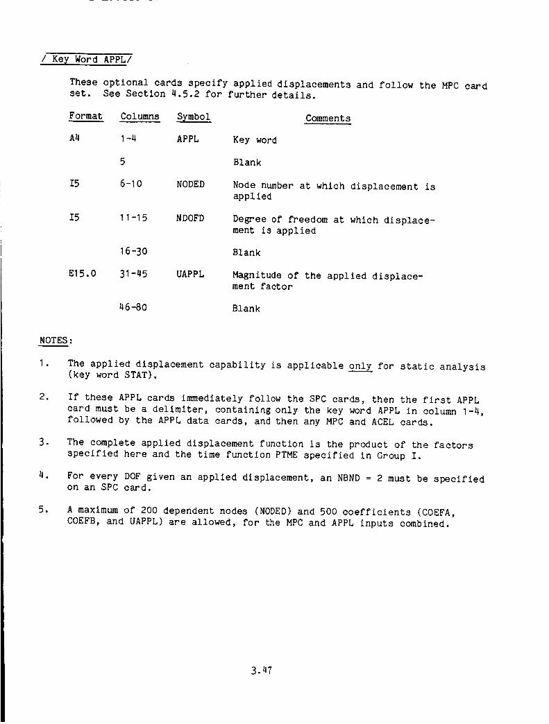
/ Key Word APPL/

These optional cards specify applied displacements and follow the MPC card

set. See Section 4.5.2 for further details.

Format Columns Symbol

A4 I-4 APPL

5

I5 6-I 0 NODED

I5 11-15 NDOFD

16-30

E15.0 31-45 UAPPL

46-80

Comments

Key word

Blank

Node number at which displacement is

applied

Degree of freedom at which displace-

ment is applied

Blank

Magnitude of the applied displace-

ment factor

Blank

NOTES :

I , The applied displacement capability is applicable only for static analysis

(key word STAT).

. If these APPL cards immediately follow the SPC cards, then the first APPL

card must be a delimiter, containing only the key word APPL in column I-4,

followed by the APPL data cards, and then any MPC and ACEL cards.

, The complete applied displacement function is the product of the factors

specified here and the time function PTME specified in Group I.

. For every DOF given an applied displacement, an NBND = 2 must be specified

on an SPC card.

. A maximum of 200 dependent nodes (NODED) and 500 coefficients (COEFA,

COEFB, and UAPPL) are allowed, for the MPC and APPL inputs combined.

3.47

/Key Word ACEL/

This optional card specifies the DOF which is given an applied

acceleration and identifies the associated table of acceleration versus time

given in Group I. One card for each DOF to be given an acceleration•

See Section 4•6.6.

Format Columns Symbol Comments

A4 I-4 ACEL Key word

5 Blank

I5 6-I 0 NODE Node given the applied acceleration

I5 11-15 NDOF DOF given the applied acceleration, I-6.

16-20 Blank

I5 21-25 ACELID Identifying number of the ACELT acceleration

vs. time function 3.108 applied to the NODE

and NDOF.

26-8O Blank

NOTES :

I • Every DOF given an applied acceleration must have its NBND = 2 on an SPC

card.

o If these ACEL cards immediately follow the SPC cards, then the first ACEL

card must be a delimiter, containing only the key word ACEL in columns I-

4, followed by the ACEL data cards, and then any MPC or APPL cards.

3. An ACELT card set is required in Group I when this ACEL card is used.

3.48

/ Key Word SEND/

This card ends the Group E data, and is always required, even if thisgroup is not used, except on a restart run.

Format Columns Symbol

A4 I-4 SEND Key word

5-80 Blank

Comments

3.49

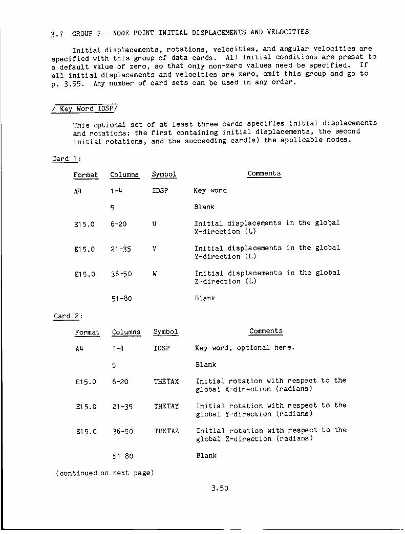
3.7 GROUP F - NODE POINT INITIAL DISPLACEMENTS AND VELOCITIES

Initial displacements, rotations, velocities, and angular velocities are

specified with this group of data cards. All initial conditions are preset to

a default value of zero, so that only non-zero values need be specified. If

all initial displacements and velocities are zero, omit this group and go to

p. 3.55. Any number of card sets can be used in any order.

/ Key Word IDSP/

This optional set of at least three cards specifies initial displacements

and rotations; the first containing initial displacements, the second

initial rotations, and the succeeding card(s) the applicable nodes.

Card I:

Format Columns Symbol Comments

A4 I-4 IDSP Key word

5 Blank

E15.0 6-20 U Initial displacements in the global

X-direction (L)

El 5.0 21 -35 V

El 5.0 36-50 W

Initial displacements in the global

Y-direction (L)

Initial displacements in the global

Z-direction (L)

Blank51 -80

El 5.0 THETAX

Card 2:

Format Columns Symbol Comments

A4 I-4 IDSP Key word, optional here.

5

6-20

E15.0 21-35 THETAY

El 5.0 36-50 THETAZ

51-80

(continued on next page)

Blank

Initial rotation with respect to the

global X-direction (radians)

Initial rotation with respect to the

global Y-direction (radians)

Initial rotation with respect to the

global Z-direction (radians)

Blank

3.50

/ Key Word IDSP/, continued from previous page

Card(s) 3:

The third and succeeding card(s) contain the applicable nodes.

Format Columns Symbol Comments

1615 1-80 NODE The applicable nodes for the above

initial displacements and rotations

are specified in fields of 5 (I5

format). The short form notation

and any number of continuation cards

may be used. A blank I5 field ends

the specifications of applicable nodes

NOTES:

I • Input need not be specified for nodes that have all their initial

displacements and rotations equal to zero.

. Displacements and rotations of constrained or dependent degrees of freedom

(NBND _ I on the SPC cards can be input here but will be ignored.

. If the llst of nodes ends in the last field on a card, a blank card mustfollow•

. Any number of sets of these cards are allowed, for the case in which

different parts of the structure have different _nitial conditions.

3.51

/ Key Word IVEL/

These optional cards specify initial velocities and angular velocities.

Each set consists of at least three cards; the first containing initial

velocities, the second initial angular velocities and the succeeding card(s)

the applicable nodes.

Card I :

Format

A4

El 5.0

Columns Symbol

I-4 IVEL

5

6-20 UDOT

El 5.0 21-35 VDOT

El 5.0 36-50 WDOT

51-80

Comments

Key word

Blank

Initial velocities in the global

X-direction (L/T)

Initial velocities in the global

Y-direction (L/T)

Initial velocities in the global

Z-dlrectlon (L/T)

Blank

Card 2:

(If Card I is used, this card must follow, even if blank.)

Columns Symbol Comments

I-4 IVEL

5

6-20 THTAXD

Format

A4

E15.0

El 5.0 21 -35 THTAYD

El 5.0 36-50 THTAZD

51-80

Key word, optional here

Blank

Initial angular velocity with

respect to the global X-direction

(PAD/T)

Initial angular velocity with

respect to the global Y-direction

(PAD/T)

Initial angular velocity with

respect to the global Z-direction

(RAD/T)

Blank

(continued on next page)

3.52

/ Key Word IVEL/, continued from previous page

Card(s) 3:

NOTES:

The third and succeeding card(s) contain the applicable nodes.

Format Columns Symbol Comments

16 I5 1-80 NODE The applicable nodes for the above

initial displacements and rotations

are specified in fields of 5 (I5

format). The short form notation

and any number of continuation cards

may be used. A blank I5 field ends

the specification of applicable nodes•

I • Input need not be specified for nodes that have all their initial

velocities equal to zero.

.

•

Velocities of constrained or dependent degrees of freedom (NBND _ I on the

SPC cards) can be input here but will be ignored.

If the list of nodes ends in the last field on a card, a blank card mustfollow.

. Any number of sets of these cards is allowed, for the case in which

different parts of the structure have different initial conditions.

3.53

/ Key Word SEND/

This card ends the Group F data, and is required only if this group is

used.

Format Columns Symbol Comments

A4 I-4 SEND Key word

5-80 Blank

NOTES :

I. Any number of card sets can be made in any order as long as each set

contains the proper internal order.

3.54

3.8 GROUPG - ADDEDINERTIA

Nodepoint lumping of structural or nonstructural concentrated massesandmassmomentsof inertia can be specified with this optional group of datacards. Whenthere are no concentrated massesor massmomentsof inertia, omitthis group and go to p. 3.58.

/ Key Word CNMI/

Each set consists of at least three cards; the first containing the mass

and eccentricities, the second mass moments of inertia, and the succeeding

card(s) the applicable nodes.

Card I:

Format Columns Symbol

A4 I-4 CNMI

5

E15.0 6-20 MASS

El 5.0 21-35 XO

El 5.0 36-50 YO

El 5.0 51 -65 ZO

66 -80

Comments

Key word

Blank

Concentrated mass at the applicablenode (M = FT2/L)

Offset distance of the mass from the

node in the global X-direction (L)

Offset distance of the mass from the

node in the global Y-direction (L)

Offset distance of the mass from the

node in the global Z-direction (L)

Blank

(continued on next page)

3.55

/ Key Word CNMI/, continued from previous page

Card 2:

Format Columns Symbol

A4 1-4 CNMI

5

El 5.0 6-20 II I

El 5.0 21 -35 I22

El 5.0 36-50 I33

51-80

Comments

Key word, optional here

Blank

Mass moment of inertia of the

concentrated ma_s about the globalX-directlon (ML_=FLT)

Mass moment of inertia of the

concentrated ma_s about the globalY-dlrection (ML_=FLT _)

Mass moment of inertia of the

concentrated ma_s about the globalZ-dlrection (ML_=FLT)

Blank

Card(s) 3:

The third and succeeding card(s) contain the applicable nodes.

Format Columns Symbol Comments

16 I5 I-80 NODE The applicable nodes for the above

concentrated mass are specified in

fields of 5 (I5 format). The short

form notation and any number of

continuation cards may be used. A

blank I5 field ends the specifica-

tion of applicable nodes.

NOTES:

I. If the list of nodes ends in the last I5 field, a blank card must follow.

1 A node having inertia added here must have no more than one independent

constraint coefficient for each of its dependent DOF, for the MPC input

specified in Group E, p 3.44.

,These items are additive. Inertia may be accumulated at a node over more

than one set of cards. A negative value will subtract inertia.

. Mass can be added or subtracted on a restart. Mass can be deleted, on a

restart, by adding negative mass here.

3.56

/ Key Word SEND/

This card ends the Group G data, and is required only if this group is

used.

Format Columns Symbol

A4 I-4 SEND

5 -8O

Key word

Blank

Comments

NOTES:

I. If this group is used on a restart, the STOP card follows immediately.

3.57

3.9 GROUP H - ELEMENT MATERIAL AND SECTION PROPERTIES

This required group consists of a number of card sets, each set initiated

by a key word. These card sets can appear in any order, although inside each

set the sequence of the cards is fixed. Data for this group can be classified

as material properties or element cross-section properties. Plastic material

properties are input in terms of yield stress and parameters that determine the

shape of a uniaxial stress versus strain curve. These parameters are defined in

Table 3.9.1 below. (Section 4.3.1) Each element must have its properties

specified in this group.

Table 3.9.1

PLASI

0.0

Et/E

Parameters Determining Hardening Behavior

PLAS2 Type of Plasticity

0.0 Ideally plastic (no strain

hardening)

0.0 Linear strain hardening, with

E t equal to the tangent modulusof the stress versus strain curve

in the plastic range

%.7 Nonlinear strain hardening

with the Ramberg-Osgood

form of the three parameter

stress versus strain curve

3a0. 7 n

o +e = g 7E

(See p. 4.19)

C-

/ Key Word MATI/

This set of at least four cards gives the material property specification

for isotropic plane stress elements, TRIM and TRP2.

Card I:

Format Columns Symbol

A4 MATI

El 5.0

E15.0

(Section 4.3.4.4)

Comments

I-4 Key word

5 Blank

6-20 E Young's modulus (F/L 2)

21-35 ANU Poisson's ratio

36-80 Blank

Card 2:

Format Columns Symbol Comments

I-5 Blank

E15.0 6-20 DENSITY Mass - density (M/L 3 = FT2/L 4)

21-50 Blank

E15.0 51-65 EPSFT Failure strain in tension (+). If

zero or blank no failure criterion

is monitored in either direction

E15.0 66-80 EPSFC

Card 3:

Format Columns Symbol

I-5

El 5.0 6-20 PLASI

E15.0 16-30 PLAS2

El 5.0 36-50 YLDST

51 -80

(continued on next page)

Failure strain in compression (-).

Use the negative sign. Ignored if

EPSFT is zero or blank.

Comments

Blank

Parameter determining plastic

hardening behavior defined in Table

3.9.1 and Section 4.3.1. Default = O.

Parameter determining plastic

hardening behavior defined in Table

3.9.1 and Section 4.3.1. Default = O.

Yield stress

Blank

3.59

/Key Word MATI/, continued from previous page

Card (s) 4 :

The fourth and succeeding card(s) contain applicable members.

Format Columns Symbol

1615 1-80 MEM

Comments

The applicable members for the above

material properties are specified in

fields of 5 (I5 format). The short

form notation and any number of

continuation cards may be used. A

blank I5 field ends the specifica-

tion of applicable members•

NOTES:

I • If a member list ends in the last I5 field of a card, a blank card mustfollow•

• Up to twenty different sets of plane stress material properties can be

specified, totalled over MATI, MAT2, MAT3.

• Non-zero tension failure (EPSFT) must be specified if failure is to be

monitored in either tension or compression• If compression failure is

desired, but tension failure is not, then use a very large strain for

EPSFT.

4. The yield stress (YLDST) must not be set to zero.

3.60

/ Key Word MAT2/

This set of at least six cards specifies plane stress material properties

for orthotropic material with orthotropic ideal plasticity (no strain

hardening). (See Section 4.3.4.4). The axes for material properties are the

orthotropic material principal directions I, 2 in the element plane, and are

assumed as a default condition to coincide with the element local coordinate

axes x, y. If these directions do not coincide, I to x and 2 to y, an

appropriate transformation angle must be input. This is discussed later in

Group H with key word MBET.

This orthotropic input is only for TRIM elements, and is currently not

operational for the TRP2 plate element.

Card I :

Format Columns Symbol Comments

A4 I-4 MAT2 Key word

5 Blank

E15.0 6-20 EONE Young's modulu_ in the material l-direction (F/L _)

E15.O 21-35 ETWO

36-50

E15.0 51-65 GONTO

El 5.0 66-80 VONTO

Young's modulu_ in the material 2-direction (F/L _)

Blank

Shear modulus for shear stresses

applied in the material I-2 directions

Poisson's ratio n12, defined

le11/e221 when e22 is applied in aas

uniaxial test

(continued on next page)

3.61

/ Key Word MAT2/, continued from previous page

Card 2 :

Format Columns Symbol Comments

I-5

El5.0 6-20 DENSITY

21-50

El5.0 51-65 EPSFTI

El 5.0 66-80 EPSFCI

Blank

Mass density (M/L 3 -- FT2/L 4)

Blank

Failure strain in tension (+) in the

material I direction. If zero or

blank no failure criterion is

monitored in either direction.

Failure strain in compression (-) in the

material I direction. The negative sign is

required. Ignored if EPSFTI is zero or blank.

Card 3:

Format Col umns Sym bo i Comments

I-5

El 5.0 6-20 EPSFT2

E15.0 21-35 EPSFC2

36 -8O

Blank

Failure strain in tension (+) in the

material 2 direction. Ignored if

EPSFTI is zero or blank.

Failure strain in compression (-) in

the material 2 direction. The

negative sign is required. Ignored ifEPSFTI is zero or blank.

Blank

Card 4 :

Format Columns Symbol Comments

I-5

El 5.0 6-20 SIGOX

E15.0 21-35 SIGOY

El 5.0 36-50 SIGOZ

El 5.0 51 -65 SIGXY

66-8O

Blank

Yiel_ stress in material 1-directlon(F/L _)

Yiel_ stress in material 2-direction(F/E L )

Yield stress in thickness-direction

(F/L 2 )

Yield stress for shear applied in the

material I-2 directions

Blank

(continued on next page)

3.62

/ Key Word MAT2/, continued from previous page

Card 5 (required)

Format Columns Symbol

I-5

El 5.0 16-20 PLASI

El 5.0 21 -35 PLAS2

36-8O

Card(s) 6:

Comments

Blank

Set equal to zero or blank

Set equal to zero or blank

Blank

The sixth and succeeding card(s) contain applicable members.

Format Columns Symbol Comments

The applicable members for the above

material properties are specified in

fields of 5 (I5 format). The short

form notation and any number of

continuation cards may be used. A

blank I5 field ends the specification

of applicable members.

NOTES :

I •

1615 1-80 MEM

.

If a member list ends in the last I5 field of a card, a blank card must

follow•

o

Up to twenty different sets of plane stress material properties can be

specified, totalled over MATI, MAT2, MAT3.

.

Non-zero tension failure (EPSFTI) must be specified if failure is to be

monitored in either tension or compression in either the material I- or 2-

directions. If no failure is desired in tension in the material I

direction, but any of the other three failures are desired, then use a

very large strain for EPSFTI.

EONE and ETWO can not be set exactly equal to zero if pure shear is being

simulated (i.e. GONTO non zero). In this case set EONE and ETWO to a

small value.

5. All values of the yield stress (card 4) must be non zero.

3.63

Ke_ Word MAT3/

This set of at least seven cards specifies plane stress material

properties for orthotropic materials with orthotroplc strain hardening (See

Section 4.3.4.4).

The axes for material properties are the orthotropic material principal

directions 1,2 in the element plane, and are assumed as a default condition to

coincide with the element local coordinate axes, x, y. If these directions do

not coincide, I to x and 2 to y, an appropriate transformation angle must be

input. This is discussed later in Group H in the set with key word MBET.

This orthotropic input is only for TRIM elements, and is currently not

operational for the TRP2 plate element.

Card I:

Format

A4

El 5.0

Columns Symbol

I-4 MAT3

5

6-20 EONE

E15.0 21-35 ETWO

36-50

E15.0 51-65 GONTO

El 5.0 66-80 VONTO

Comments

Key word

Blank

Young's modulu_ in the material l-direction (F/L _)

Young's modulu_ in the material 2-direction (F/L c)

Blank

Shear modulus for shear stresses

applied in the material I-2 directions

Poisson's ratio n12, defined as

le11/e221 when e22 is applied in auniaxial test

(continued on next page)

3.64

/ Key Word MAT3/, continued from previous page

Card 2:

Format Columns Symbol Comments

I-5

El 5.0 6-20 DENSITY

21 -50

Blank

Mass density (M/L 3 = FT2/L 4)

Blank

El 5.0 51 -65 EPSFT I Failure strain in tension (+) in the

material I direction. If zero or blank

no failure criterion is monitored in

in either direction.

El 5.0 66-80 EPSFCI

Card 3:

Failure strain in compression (-) in the

material I direction. Negative sign

required. Ignored if EPSFTI is zero or blank.

Format Columns Symbol Comments

I-5 Blank

El 5.0 6-20 EPSFT2 Failure strain in tension (+) in the

material 2 direction. Ignored if EPSFTI

is zero or blank.

El 5.0 21 -35 EPSFC2 Failure strain in compression (-) in the

material 2 direction. Negative sign required.

Ignored if EPSFTI is zero or blank.

36-8O Blank

Card 4:

Format Columns Symbol Comments

I-5 Blank

El 5.0 6-20 SIGOX Yiel_ stress in material l-direction(F/L =)

El 5.0 21 -35 SIGOY Yiel_ stress in material 2-direction(F/L L )

El 5.0 36-50 SIGOZ Yield stress in thickness-direction

(F/L 2)

E15.0 51-65 SIGXY

65-80

Shear yiel_ stress in principal I-2

plane (F/L z)

Blank

3.65

/ Cards : Key Word MAT3/, continued from previous page

Card 5:

Format Columns Symbol Comments

I-5

El 5.0 6-20 PLASI X

El 5.0 21 -35 PLAS2X

E15.0 36-50 PLASIY

El 5.0 51 -65 PLAS2Y

El 5.0 66-80 PLASI XY

Card 6:

Format Columns Symbol

Blank

Same as PLASI (Table 3.9.1) but for

material l-direction only, nonzero

Same as PLAS2 (Table 3.9.1) but for

material l-direction only.

Same as PLASI (Table 3.9.1) but for

material 2-direction only, nonzero

Same as PLAS2 (Table 3.9.1) but for

material 2-direction only.

Same as PLASI (Table 3.9.1) but for

shear applied in the material I-2

directions only, nonzero

I-5

El 5.0 6-20 PLAS2XY

16-80

Comments

Blank

Same as PLAS2 (Table 3.9.1) but for

shear applied in material I-2

directions only.

Blank

(continued on next page)

3.66

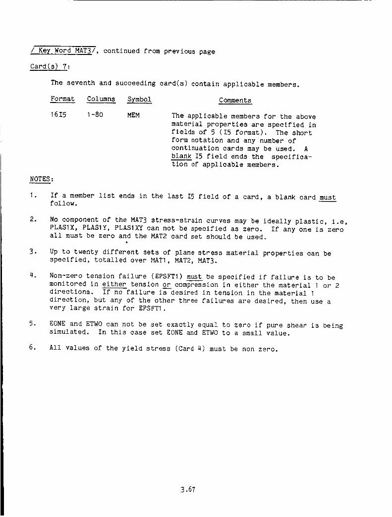
/.Key Word MAT3/, continued from previous page

Card(s) 7:

The seventh and succeeding card(s) contain applicable members•

Format Columns Symbol Comments

1615 1-80 MEM The applicable members for the above

material properties are specified in

fields of 5 (I5 format). The short

form notation and any number of

continuation cards may be used. A

blank I5 field ends the specifica-

tion of applicable members.

NOTES:

I • If a member list ends in the last I5 field of a card, a blank card mustfollow•

1

•

No component of the MAT3 stress-strain curves may be ideally plastic, i.e,

PLASIX, PLASIY, PLASIXY can not be specified as zero. If any one is zeroall must be zero and the MAT2 card set should be used.

Up to twenty different sets of plane stress material properties can be

specified, totalled over MATI, MAT2, MAT3.

. Non-zero tension failure (EPSFTI) must be specified if failure is to be

monitored in either tension or compression in either the material I or 2

directions. If no failure is desired in tension in the material I

direction, but any of the other three failures are desired, then use a

very large strain for EPSFTI.

1 EONE and ETWO can not be set exactly equal to zero if pure shear is beingsimulated. In this case set EONE and ETWO to a small value.

6. All values of the yield stress (Card 4) must be non zero.

3.67

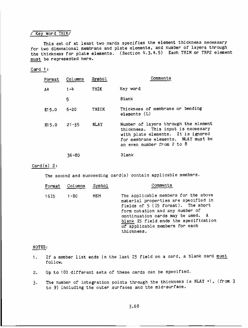
/ Key Word THIK/

This set of at least two cards specifies the element thickness necessary

for two dimensional membrane and plate elements, and number of layers through

the thickness for plate elements. (Section 4.3.4.5) Each TRIM or TRP2 element

must be represented here.

Card I :

Format Columns STmbol

A4 I-4 THIK Key word

Comments

5 Blank

El 5.0 6-20 THICK Thickness of membrane or bending

elements (L)

El 5.0 21 -35 NLAY Number of layers through the element

thickness. This input is necessary

with plate elements. It is ignored

for membrane elements. NLAY must be

an even number from 2 to 8

36-80 Blank

Card(s) 2:

The second and succeeding card(s) contain applicable members.

Format Columns Symbol Comments

1615 I-80 MEM The applicable members for the above

material properties are specified in

fields of 5 (I5 format). The short

form notation and any number of

continuation cards may be used. A

blank I5 field ends the specification

of applicable members for each

thickness.

NOTES:

I . If a member list ends in the last I5 field on a card, a blank card mustfollow.

2. Up to 100 different sets of these cards can be specified.

o The number of integration points through the thickness is NLAY +I, (from 3

to 9) including the outer surfaces and the mid-surface.

3.68

/ Key Word MBET/

This optional set of at least two cards specifies the orientation of axes

of material anisotropy for TRIM elements. Not required for any element when

the element's material I axls coincide with its local x axis.

4.3.4.6)

Card I:

Format Columns Symbol Comments

A4 MBETI-4

5

El 5 .0 6-20 BETF

(Section

21 -80

Card(s) 2:

Key word

Blank

Angle in de_rees between element

local X-axis and principal 1-axls

for material orthotropy. (Degrees)

Blank

The second and succeeding card(s) contain applicable members.

Format Columns Symbol Comments

The applicable members for the above

angles are specified in fields of 5

(I5 format). The short form nota-

tion and any number of continuation

cards may be used. A blank I5 field

ends the specification of applicablemembers.

1615 1-80 MEM

NOTES:

I ,

.

If a member list ends in the last I5 field on a card, a blank card mustfollow.

An orientation angle can be specified for any TRIM element in a model.

an element is not listed here, its material orientation angle BETF willdefault to zero.

If

3.69

/ Key Word MSTG/

This set of three or more cards specifies material and section properties

for stringer elements (axial force elements).

(STRG) elements are used. (Section 4.3.2.4)

represented here.

Card I :

Format Columns Symbol

A4 1-4 MSTG

5

El 5.0 6-20 E

E15.0 21-35 A

El 5.0 36-50 PLASI

El 5.0 51 -65 PLAS2

E15.0 66-8O

Card 2:

Format Columns

YLDST

Symbol

I-5

El5 .0 6-20 DENSITY

21 -35

El 5.0 36-50 SEPST

El 5.0 51 -65 SEPSC

66-80

Necessary only when stringer

Each STRG element must be

Comments

Key word

Blank

Young's modulus (F/L 2)

Cross sectional area (L2)

Parameter determining plastic

hardening behavior defined in Table 3.9.1

and Section 4.3.1

Parameter determining plastic

hardening behavior defined in Table 3.9.1

and Section 4.3.1

Yield stress (F/L 2)

Comments

Blank

Mass-density (M/L 3 _ FT2/L 4)

Blank

Failure strain in tension (+). If

zero or blank no failure criterion

is monitored in tension or compres-

sion.

Failure strain in compression (-). Negative

sign required. Ignored if SEPST is zero or

blank.

Blank

(continued on next page)

3.70

/ Key Word MSTG/, continued from previous page

Card(s) 3:

The third and succeeding card(s) contain applicable members.

Format Columns Symbol Comments

1615 I-80 MEM The applicable members for the above

material properties are specified in

fields of 5 (I5 format). The short

form notation and any number of

continuation cards may be used. A

blank I5 field ends the specifica-

tion of applicable members.

NOTES:

I • If a member list ends in the last I5 field on a card, a blank card must

follow.

. Up to 200 different sets of MSTG and beam section geometry (CSEC, etc.)

card sets can be specified.

. Non-zero tension failure (SEPST) must be specified if failure is to be

monitored in either tension or compression. If no tension failure is

desired, but compression failure is desired, use a very large strain for

SEPST.

3.71

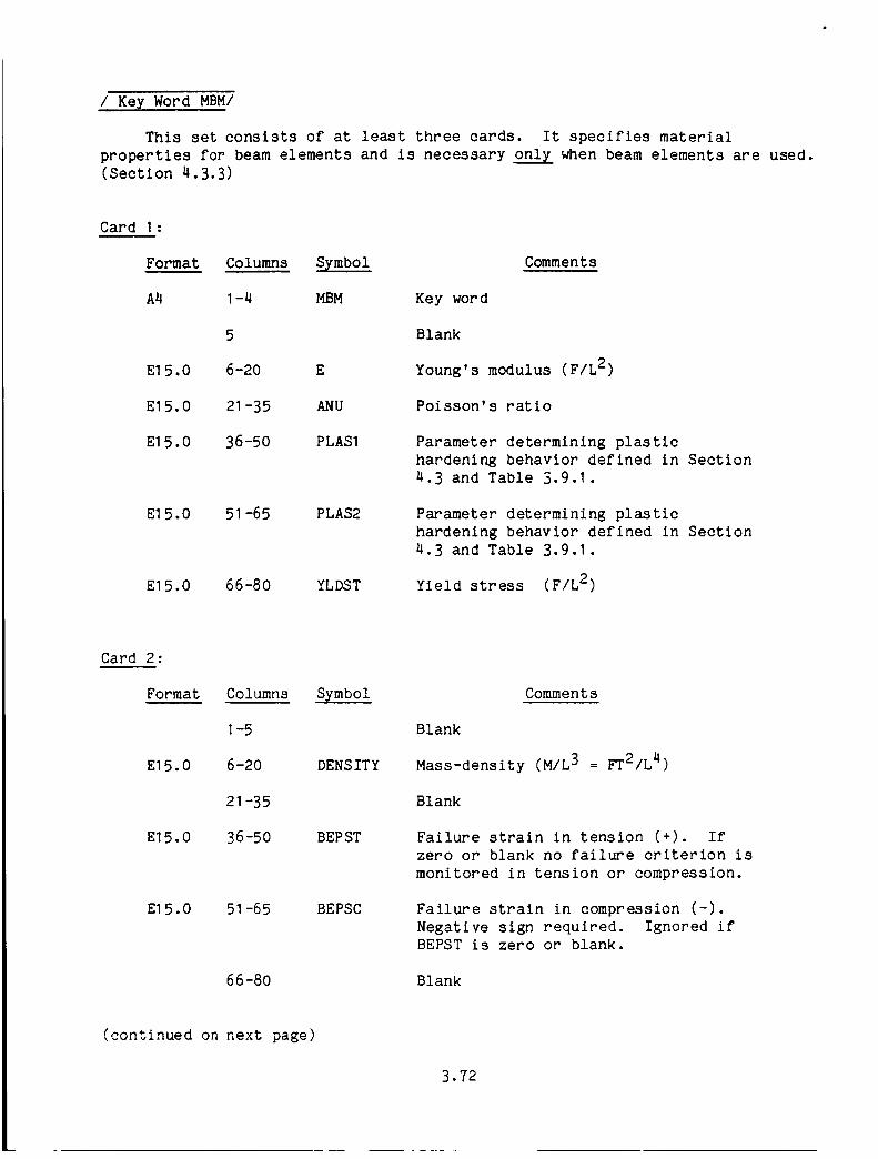
/ Key Word MBM/

This set consists of at least three cards. It specifies material

properties for beam elements and is necessary only when beam elements are used.

(Section 4.3.3)

Card I:

Format

A4

El 5.0

E15.0

El 5.0

Columns Symbol

I-4 MBM

5

6-20 E

21-35 ANU

36-50 PLASI

E15.0 51-65 PLAS2

El 5.0 66-80 YLDST

Comments

Key word

Blank

Young's modulus (F/L 2)

Poisson's ratio

Parameter determining plastic

hardening behavior defined in Section

4.3 and Table 3.9.1.

Parameter determining plastic

hardening behavior defined in Section

4.3 and Table 3.9.1.

Yield stress (F/L 2)

Card 2:

Format Columns Symbol

I-5

El 5.0 6-20 DENSITY

21 -35

E15.0 36-50 BEPST

El 5.0 51 -65 BEPSC

66-8O

Comments

Blank

Mass-density (M/L 3 = FT2/L 4)

Blank

Failure strain in tension (+). If

zero or blank no failure criterion is

monitored in tension or compression.

Failure strain in compression (-).

Negative sign required. Ignored if

BEPST is zero or blank.

Blank

(continued on next page)

3.72

/ Key Word MBM/, continued from previous page

The succeeding card(s) contain the applicable members.

Card(s) 3: Applicable Members :

Format Columns Symbol Comments

1615 I-80 MEM The applicable members for the above

beam material properties are specified

in fields of 5 (I5 format). The short

form notation and any number of

continuation cards may be used. A

blank I5 field ends the specification

of applicable members.

NOTES:

I. Up to 50 different MBM sets can be specified.

. If a member list ends in the last I5 field on a card, a blank card must

follow.

. Non-zero tension failure (BEPST) must be specified if failure is to be

monitored in either tension or compression. If tension failure is not

desired, but compression fail--ure is desired, use a very large strain for

BEPST.

. Poisson's ratio on card I is used only to calculate the elastic shear

modulus G = E/2(I + _).

3.73

/ Special Beam Sections/

This set of at least four cards specifies the geometric properties for the

special beam cross sections having certain fixed shapes. The listed key words

refer to various beam cross sections defined in Section 4.3.3.5 and Table

4.3.1.

The key words are: CSEC, HCIR, HREC, HSEC, ISEC, LSEC, LSEG, SCIR, SREC, TSEC,

TWD, ZSCR, ZSEC.

The first two cards have the same format for all the special sections, and will

be described here only once.

Card i :

Format

A4

Columns

I-4

Symbol Comments

Appropriate special beam section key word

from above list.

E15.0

El 5.0

E15.0

E15.0

E15.0

5

6-20

21-35

36-50

51-65

66-80

A

IYY

IZZ

IYZ

J

Blank

Cross sectional area (L2)

Moment of inertia about centroidal y-axis (L 4)

Moment of inertia about centroidal z-axis (L4)

Product of inertia about centroidal y-z axes (L4)

Torsional rigidity (L 4)

NOTES:

I . A, IYY, IZZ and IYZ will be internally calculated if all four are set to

zero or blank in the Input data. However, J must always be input, except

for the TWD section, where it is ignored.

(continued on next page)

3.74

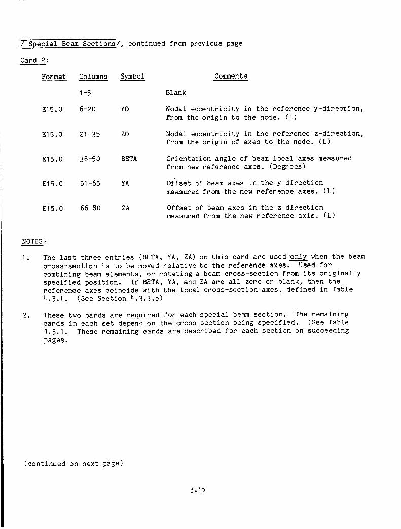
/ Special Beam Sections/, continued from previous page

Card 2:

Format Columns Symbol Comments

I-5 Blank

El 5 •0 6-20 YO Nodal eccentricity in the reference y-direction,

from the origin to the node. (L)

E15.0 21-35 ZO Nodal eccentricity in the reference z-direction,

from the origin of axes to the node. (L)

El 5.0 36-50 BETA

E15.0 51-65 YA

Orientation angle of beam local axes measured

from new reference axes. (Degrees)

Offset of beam axes in the y direction

measured from the new reference axes. (L)

E15.0 66-80 ZA Offset of beam axes in the z direction

measured from the new reference axis. (L)

NOTES:

I , The last three entries (BETA, YA, ZA) on this card are usedonly when the beam

cross-section is to be moved relative to the reference axes. Used for

combining beam elements, or rotating a beam cross-section from its originally

specified position. If BETA, YA, and ZA are all zero or blank, then the

reference axes coincide with the local cross-section axes, defined in Table

4.3.1. (See Section 4.3.3.5)

. These two cards are required for each special beam section. The remaining

cards in each set depend on the cross section being specified. (See Table

4.3.1. These remaining cards are described for each section on succeeding

pages.

(continued on next page)

3.75

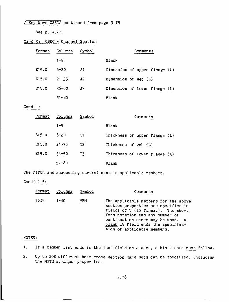
/ Key Word CSEC/ continued from page 3.75

See p. 4.47.

Card 3: CSEC - Channel Section

Format Columns Symbol

I-5

El 5 •0 6-20 AI

El 5.0 21 -35 A2

El 5.0 36-50 A3

51 -8O

Card 4:

Format Columns Symbol

I-5

El 5.0 6-20 TI

E15.0 21 -35 T2

El 5.0 36-50 T3

51-80

Comments

Blank

Dimension of upper flange (L)

Dimension of web (L)

Dimension of lower flange (L)

Blank

Comments

Blank

Thickness of upper flange (L)

Thickness of web (L)

Thickness of lower flange (L)

Blank

The fifth and succeeding card(s) contain applicable members.

Card(s) 5:

Format Columns Symbol Comments

1615 1-80 MEM The applicable members for the above

section properties are specified in

fields of 5 (I5 format). The short

form notation and any number of

continuation cards may be used. A

blank I5 field ends the specifica-

tion of applicable members.

NOTES:

I. If a member list ends in the last field on a card, a blank card must follow.

o Up to 200 different beam cross section card sets can be specified, including

the MSTG stringer properties.

3.76

/ Ke_ Word HCIR/ continued from page 3.75

See p. 4.48.

Card 3: HCIR - Hollow Circle

Format Columns Symbol

I-5

El 5.0 6-20 R

El 5.0 21-35 T

36-80

Comments

Blank

Outer radius (L)

Thickness (5)

Blank

The fourth and succeeding card(s) contain applicable members.

Card(s) 4:

Format Columns Symbol

1615 1-80 MEM

Comments

The applicable members for the above

section properties are specified in

fields of 5 (I5 format). The short form

notation and any number of continuation

cards may be used. A blank I5 field ends

the specification of applicable members.

NOTES:

I. If a member list ends in the last field on a card, a blank card must follow.

2. Up to 200 different beam cross section card sets can be specified, including

the MSTG stringer properties.

3.77

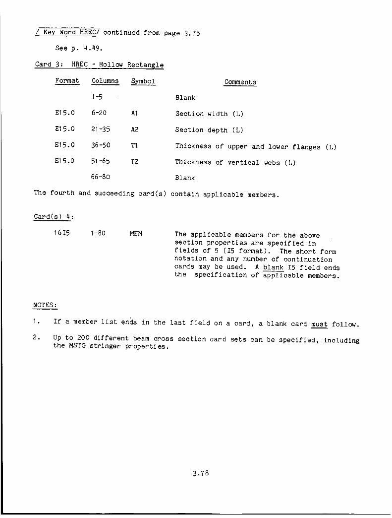
/ Key Word HREC/ continued from page 3.75

See p. 4.49.

Card 3: HREC - Hollow Rectangle

Format Columns Symbol

I-5

El 5.0 6-20 AI

El 5.0 21-35 A2

El 5 •0 36-50 TI

El 5.0 51-65 T2

66-80

Comments

Blank

Section width (L)

Section depth (L)

Thickness of upper and lower flanges (L)

Thickness of vertical webs (L)

Blank

The fourth and succeeding card(s) contain applicable members.

Card(s) 4:

16 I5 1-80 MEM The applicable members for the above

section properties are specified in

fields of 5 (15 format). The short form

notation and any number of continuation

cards may be used. A blank I5 field ends

the specification of applicable members.

NOTES :

I. If a member list ends in the last field on a card, a blank card must follow.

2. Up to 200 different beam cross section card sets can be specified, including

the MSTG stringer properties.

3.78

/ Key Word HSEC/ continued from page 3.75

See p. 4.50.

Card 3: HSEC - Hat Section

Format Columns Symbol

I-5

El5 •0 6-20 B

E15.0 21 -35 BI

E15.0 36-50 H

El 5.0 51-65 T

66-80

The fourth and succeeding card(s) contain applicable members.

Comments

Blank

Dimension of flanges (L)

Dimension of flange tabs (L)

Dimension of web (L)

Uniform Section thickness (L)

Blank

Card(s) 4:

Format Columns Symbol

1615 1-80 MEM

Comments

The applicable members for the above

section properties are specified in

fields of 5 (I5 format). The short

form notation and any number of

continuation cards may be used. A

blank I5 field ends the specifica-

tion of applicable members.

NOTES:

I .

2.

If a member list ends in the last field on a card, a blank card must follow.

Up to 200 different beam cross section card sets can be specified, including

the MSTG stringer properties.

3.79

/ Key Word ISEC/ continued from page 3.75

See p. 4.51.

Card 3: ISEC - I-Section

Format Columns Symbol

E15.0

El 5.0

E15.0

Card 4:

Format

I-5

6-20 AI

21 -35 A2

36-50 A3

51-8O

Columns Symbol

I-5

E15.0 6-20 TI

El 5.0 21 -35 T2

E15.0 36-50 T3

51 -8O

Comments

Blank

Dimension of upper flange (L)

Dimension of web (L)

Dimension of lower flange (L)

Blank

Comments

Blank

Thickness of upper flange (L)

Thickness of web (L)

Thickness of lower flange (L)

Blank

The fifth and succeeding card(s) contain applicable members.

Card(s) 5:

Format Columns Symbol Comments

16 I5 I-80 MEM The applicable members for the above

section properties are specified in

fields of 5 (I5 format). The short

form notation and any number of

continuation cards may be used. A

blank I5 field ends the specifica-

tion of applicable members.

NOTES :

I. If a member list ends in the last field on a card, a blank card must follow.

, Up to 200 different beam cross section card sets can be specified, including

the MSTG stringer properties.

3.80

/ Key Word LSEC/ continued from page 3.75

See p. 4.52.

Card 3: LSEC - L-Section

Format Columns Symbol Comments

I-5 Blank

E15.0 6-20 AI Width of flange (L)

E15.0 21-35 A2 Depth of web (L)

E15.0 36-50 TI Thickness of flange (L)

E15.0 51-65 T2 Thickness of web (L)

66-80 Blank

The fourth and succeeding card(s) contain applicable members.

Card(s) 4:

Format Columns Symbol

1615 1-80 MEM

Comments

The applicable members for the above

section properties are specified in

fields of 5 (I5 format). The short form

notation and any number of continuation

cards may be used. A blank I5 field ends

the specification of applicable members.

NOTES:

I •

2.

If a member list ends in the last field on a card, a blank card must follow.

Up to 200 different beam cross section card sets can be specified, including

the MSTG stringer properties.

3.81

/ Key Word LSEG/, continued from page 3.75

See p. 4.53.

Card 3 :

Format

A4

E15.0

El 5.0

E15.0

E15.0

LSEG - Line Segment (Thin Rectangle)

Columns Symbol

1-4 LSEG

5-IO

11-25 YI

26-40 ZI

41-55 Y2

56 -7O Z2

71 -80

Comments

Key word, optional here

Blank

Y coordinate of start point (L)

Z coordinate of start point (L)

Y coordinate of end point (L)

Z coordinate of end point (L)

Blank

Card 4:

Format

A4

El 5.O

E15.0

NOTES :

I ,

This card must follow its associated card 3.

Columns

I-4

5-I0

I1-25

26-4O

Symbol

LSEG

T

NINT

41-80

Comments

Key word, optional here

Blank

Segment thickness (L)

Number of Gauss integration points

in the segment. From 2 to 8 are

allowed.

Blank

This element has no bending stiffness about the axis through the starting and

ending points.

(continued on next page)

3.82

/ Key Word LSEG/, continued from previous page

The succeeding card(s) contain applicable members.

Card(s) 5:

Format Columns Symbol

16I5 I-80 MEM

Comments

The applicable members for the above

section properties are specified infields of 5 (I5 format). The short

form notation and any number of

continuation cards may be used. A

blank I5 field ends the specificationof applicable members.

NOTES :

I. If a member list ends in the last field on a card, a blank card must follow.

2. Up to 200 different card sets of beam cross-sections can be specified,

including the MSTG stringer properties.

3.83

/ Key Word SCIR/ continued from page 3.75

See p. 4.54.

Card 3: SCIR - Solid Circle

Format Columns Symbol

I-5

E15.0 6-20 R

21-80

Comments

Blank

Section radius (L)

Blank

The fourth and succeeding card(s) contain applicable members.

Card(s) 4:

Format Columns Symbo !

1615 1-80 MEM

NOTES :

I .

2.

Comments

The applicable members for the above

section properties are specified in

fields of 5 (I5 format). The short

form notation and any number of

continuation cards may be used. A

blank I5 field ends the specifica-

tion of applicable members.

If a member list ends in the last field on a card, a blank card must follow.

Up to 200 different beam cross section card sets can be specified, including

the MSTG stringer properties.

3.84

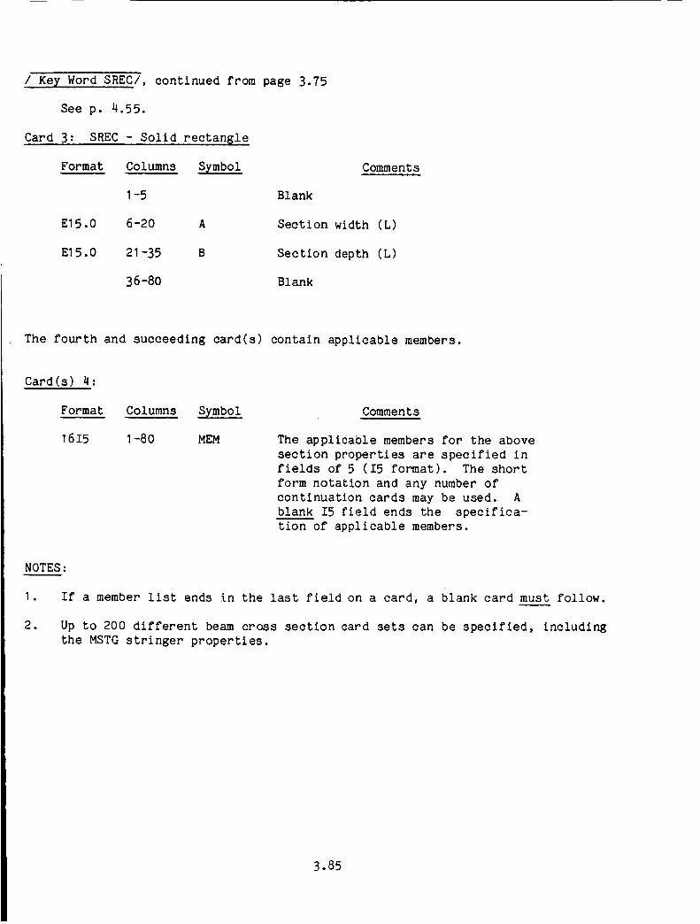
/ Key Word SREC/, continued from page 3.75

See p. 4.55.

Card 3: SREC - Solid rectangle

Format Columns Symbol

I-5

E15.0 6-20 A

El 5.0 21 -35 B

36-80

Comments

Blank

Section width (L)

Section depth (L)

Blank

The fourth and succeeding card(s) contain applicable members.

Card(s) 4:

Format Columns Symbol

1615 1-80 MEM

Comments

The applicable members for the above

section properties are specified in

fields of 5 (I5 format). The short

form notation and any number of

continuation cards may be used. A

blank I5 field ends the specifica-

tion of applicable members.

NOTES:

I. If a member list ends in the last field on a card, a blank card must follow.

2. Up to 200 different beam cross section card sets can be specified, including

the MSTG stringer properties.

3.85

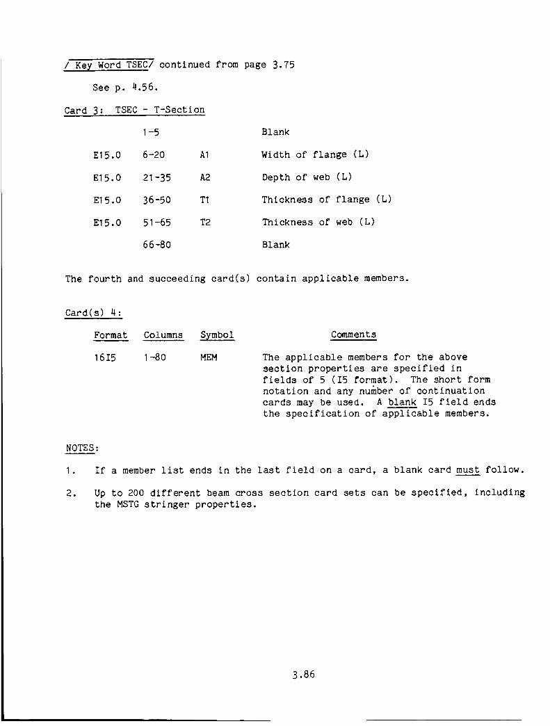
/ Key Word TSEC/ continued from page 3.75

See p. 4.56.

Card 3: TSEC - T-Section

I-5

El 5.0 6-20 AI

E15.0 21 -35 A2

El 5.0 36-50 TI

E15.0 51-65 T2

66-80

Blank

Width of flange (L)

Depth of web (L)

Thickness of flange (L)

Thickness of web (L)

Blank

The fourth and succeeding card(s) contain applicable members.

Card(s) 4 :

Format Columns Symbol

1615 1-80 MEM

Comments

The applicable members for the above

section properties are specified in

fields of 5 (I5 format). The short form

notation and any number of continuation

cards may be used. A blank I5 field ends

the specification of applicable members.

NOTES:

I. If a member list ends in the last field on a card, a blank card must follow.

2. Up to 200 different beam cross section card sets can be specified, including

the MSTG stringer properties.

3.86

/ Key Word TWD/ continued from page 3.75

See p. 4.57.

Card 3: TWD - Two Dimensional Section

Format Columns Symbol Comments

I-5 Blank

El 5.0 6-20 W Section width (perpendicular to the

plane of motion) (L)

El 5.0 21 -35 T Section depth or thickness (L)

E15.0 36-50 NLAY Defines the number of integration

points through the section depth.

NLAY is the number of layers through

the thickness in a Simpson's rule

integration. NLAY must be an even

number < 58

51-80 Blank

The fourth and succeeding card(s) contain applicable members.

Card(s) 4:

Format Columns Symbol Comments

1615 I-80 MEM The applicable members for the above

section properties are specified in

fields of 5 (I5 format). The short

form notation and any number of

continuation cards may be used. A

blank I5 field ends the specifica-

tion of applicable members.

NOTES:

I • This beam calculates no bending stiffness in the local y direction, nor

torsional stiffness. That is, the internal calculations will define zero

values for IZZ, IYZ, and J. Finite values for those parameters can be

specified in the first card of this set, but these values will be main-tained

only in the elastic range. As soon as any integration point becomes plastic at

either node, the internal calculations will take over, and the zero values will

be used.

2. If a member list ends in the last field on a card, a blank card must follow.

• Up to 200 different beam cross section card sets can be specified, including

the MSTG stringer properties.

3.87

/ Key Word ZSCR/ continued from page 3.75

See p. 4.58.

Card 3: ZSCR - Reversed Z-Section

Format Columns Symbol

I-5

El 5 •0 6-20 AI

El 5.0 21 -35 A2

El 5.0 36-50 A3

51-80

Card 4:

Format Columns Symbol

I-5

El 5 •0 6-20 TI

El 5.0 21-35 T2

El 5.0 36-50 T3

51 -8O

Comments

Blank

Dimension of upper flange (L)

Dimension of web (L)

Dimension of lower flange (L)

Blank

Comments

Blank

Thickness of upper flange (L)

Thickness of web (L)

Thickness of lower flange (L)

Blank

The fifth and succeeding card(s) contain applicable members.

Card(s) 5:

Format Columns Symbol Comments

1615 1-80 MEM

NOTES:

I •

The applicable members for the above

section properties are specified in

fields of 5 (I5 format). The short

form notation and any number of

continuation cards may be used. A

blank I5 field ends the specifica-

tion of applicable members.

If a member list ends in the last field on a card, a blank card must follow•

. Up to 200 different beam cross section card sets can be specified, including

the MSTG stringer properties.

3. The upper and lower flanges must be equal; AI = A 3, T I = T3.

3.88

/ Key Word ZSEC/ continued from page 3.75

See p. 4.59.

Card 3: ZSEC - Z-Section

Format Columns Symbol

I-5

El5.0 6-20 AI

El5.0 21 -35 A2

El5.0 36-50 A3

51-8O

Card 4:

Format Columns Symbol

I-5

El5.0 6-20 TI

E15.0 21 -35 T2

El 5.0 36-50 T3

51 -8O

Comments

Blank

Dimension of upper flange (L)

Dimension of web (L)

Dimension of lower flange (L)

Blank

Comments

Blank

Thickness of upper flange (L)

Thickness of web (L)

Thickness of lower flange (L)

Blank

The fifth and succeeding card(s) contain applicable members.

Card(s) 5:

Format Columns Symbol

1615 1-80 MEM

NOTES:

Comments

The applicable members for the above

section properties are specified infields of 5 (I5 format). The short

form notation and any number of

continuation cards may be used. A

blank I5 field ends the specifica-

tion of applicable members.

I • If a member list ends in the last field on a card, a blank card must follow.

. Up to 200 different beam cross section card sets can be specified, including

the MSTG stringer properties.

3. The upper and lower flanges must be equal; AI --A3, TI-- T3

3.89

/ Key Word PSPR/

This set of at least four cards specifies nonlinear spring properties for

spring elements and is necessary only when spring elements are used. Input is

in the form of force versus elongation or moment versus rotation tables.

(Section 4.3.5 p. 4.81).

Card I:

Format Columns Symbol Comments

A4 I-4 PSPR Key word

Blank

El 5.0 6-20 NSPRG The number of points in the table, from 2

to 20.

E15.0 21-35 USPRG Unloading slope. If zero or blank,

unloading follows loading curve (no

energy dissipation). If nonzero,

unloading follows along the

unloading slope. (F/L or FL/L)

E15.0 36-50 FAILT Tension failure elongation or rotation (*).If zero or blank no failure

criterion is monitored in either

direction. (L or radians)

E15.0 51 -65 FAILC Compression failure elongation or rotation

(-). Use the negative sign. (L or radians)

E15.0 66-80 DMASS A characteristic mass used to calculate

damping. If DMASS i_ blank or zero there is

no damping. (M = FTC/L) See p. 4.86.

(Section 4.3.5.4) Note 3.

NOTES:

I , DMASS defines a special type of nonlinear critical damping that was designed to

be used with springs acting as gap elements, to prevent rapid oscillations at

the contact point. See p. 4.88.

. Non-zero tension failure elongation (FAILT) must be specified if failure is to

be monitored in either tension or compression. If tension failure is not

desired, but compression failure is desired, use a very large force or momentfor FAILT.

3. Damping is not operational with the explicit time integrators ADAM and CDIF.

(continued on next page)

3.90

/ Key Word PSPR/ continued from previous page

Cards 2:

These cards specify spring force and elongation in pairs, one pair on each

card. There should be a total of NSPRG cards specified, i.e, one for each

point in the table of force versus elongation (or moment vs rotation). A

minimum of two such cards is required, and a maximum of 20 are allowed.

The data must be input in order of increasing elongation, i.e, from largest

negative elongation, through zero, to largest positive elongation. Zero

elongation must be included in this table (but zero force is not required).

There are no restrictions on the variation of forces.

Format Columns Symbol Comments

A4 I-4 PSPR Key word, optional here

5 Blank

E15.0 6-20 FORCE Spring force (F) or moment (FL)

E15.0 21-35 ELONG Spring elongation (L) or rotation (Radians)

36-80 Blank

The succeeding card(s) contain the applicable members.

Card(s) 3:

Format Columns Symbol Comments

16 I5 I-80 MEM The applicable members for the above spring

table properties are specified in fields of 5

(I5 format). The short form notation and any

number of continuation cards may be used.

A blank I5 field ends the specification of

applicable members.

NOTES:

I. If a member list ends in the last field on a card, a blank card must follow.

2. A total of 60 PSPR and PGRD tables are allowed, with a maximum of 20 points per

table.

3.91

/ Key Word PGRD/

This set of at least seven cards specifies the properties of all the ground

contact springs (GRDS) that will contact a single specified contact plane. One

set is required for each contact plane, whenever any GRDS elements are used.

(See Section 4.3.7.4 p. 4.108).

Card I :

Format Columns Symbol Comments

A4 1 -4 PGRD Key word, required here.

Blank

El 5.0 6-20 NSPRG Number of force-displacement points, from

2. to 20.

El 5.0 21 -35 FRICT Coefficient of sliding friction. Note I.

El 5.0 36-50 EPSC Contact tolerance. Default = Infinity. (L)

E15.0 51-65 EPSR Rebound tolerance. Default = O. (L)

El 5.0 66-80 DMASSCharacteristic mass used to calculatedamping force. Note 2. (M = FT /L)

NOTES :

I , There is no static friction. When the sliding velocity of a node along the

contact plane is zero, or the STAT time integrator is used in Group A, the

friction force is zero.

. DMASS defines a "damping mass" for a special type of critical damping designed

to be used with gap springs, to prevent rapid oscillations at the contact

point. Damping is not operational for the explicit time integrators ADAM andCDIF.

(continued on next page)

3.92

/ Key Word PGRD/ continued from previous page

Cards 2:

This subset of three cards specifies the three points that define a contact

plane, and are required for every PGRD input set. Each card contains the

global coordinates of one such point. The three cards have identical formats,

as follows (Section 4.3.7.4):

Format Columns

A4 I-4

5

El 5 •0 6-20

E15.0 21 -35

El 5.0 36-50

51 -80

Symbol

PGRD

COORDX

COORDY

COORDZ

Comments

Key word, optional here.

Blank

Global X coordinate• (L)

Global Y coordinate. (L)

Global Z coordinate. (L)

Blank

NOTES :

I • The three points define a local X', Y', Z' coordinate system as follows: the

local X' axis lles in the plane, from the first point towards _the second

point. The local Y' axis lies in the plane, is perpendicular to the local X'

axis and passes through the third point• The local Z' axis is perpendicular to

the X', Y' plane in the positive direction as defined by the right-hand rule.

The local Z' axis must be on the same side of the X', Y' plane as the contact

nodes. In other words, all the contact nodes must be on the same side of the

contact plane X' Y', as the Z axis. This direction of the Z' axis is

determined by the sequence of the three nodes in the input stream, and the user

should be careful to insure the proper sequence. See Fig. 4.3.11, p. 4.109.

(continued on next page)

3.93

/ Key Word PGRD/ continued from previous page

Cards 3:

This subset of at least two cards contains the number of cards equal to the

value of NSPRG on card I, that is, one card for each data point in the force-

displacement curve for the contact springs to the contact surface defined by

cards 2. A maximum of 20 cards is permitted. The format of each card is

identical, as follows (Section 4.3.7.4):

Format Columns Symbol Comments

A4 1-4 PGRD Key word, optional here.

5 Blank

El 5.0 6-20 FOR CE Contact force. Use a positive value.

Note I.(F)

El 5.0 21-35 ELONG Contact displacement. Use a positive

value. Note I (L)

36-80 Blank

NOTES :

I , These are compression forces and displacements. They will be converted to

negative values internally.

. The ELONG values must increase monotonically from zero with each succeeding

card, but the FORCE values can vary without restriction. The curve is

extrapolated to infinity from the last input point using the last slope.

(continued on next page)

3.94

/ Key Word PGRD/ continued from previous page

The remaining card(s) of this set contain(s) the identification of the GRDS

elements for which the above data applies.

Format Columns Symbol Comments

16I5 I-80 MEM The list of applicable members in fields

of 5 (I5 format). The short form notation

and any number of cards are allowed. A blank

I5 field ends this list.

NOTES:

I. If this list ends in the last field on a card, a blank card must follow.

2. A total of 60 PSPR and PGRD tables are allowed, with a maximum of 20 points pertable.

3.95

/ Key Word SEND/

This required card ends the Group H data.

Format Columns Symbol

A4 I-4 SEND Key word

5-80 Blank

Comments

NOTES :

3.96

3.10 Group I - Applied loading

This optional groups specifies external loads and their associated timefunctions. These include; point, line, and area loads, time functions for theseloads, and gravity loads which have a built-in step-function in time. Alsospecified here are applied acceleration versus time functions.

The input card sets may appear in any order but within each set, the order isfixed. Section 4.6 describes the applied load capability.

If there are no applied loads or accelerations go to the last card (STOPorEND), p. 3.111.

3.97

I Key Word CONCI

This optional set of at least two cards specifies the concentrated nodal forces

and moments. These loads remain attached to their nodes, and maintain their

initial directional orientation relative to the global X, Y, Z axes. (Section

4.6.1)

Card I:

Format

A4 I-4

5

I5 6-I 0 NODE

E15.0 11-25 FX

El 5.0 26-40 FY

El 5.0 41 -55 FZ

56-8O

Columns Symbol Comments

CONC Key word

Blank

Node number

Force factor in global X-direction (F)

Force factor in global Y-direction (F)

Force factor in global Z-direction (F)

Blank

Card 2:

Format Columns Symbol

A4 I-4 CONC

5-I0

E15.0 11-25 MX

E15.0 26-40 MY

E15.0 41-55 MZ

56-80

Comments

Key word, optional here

Blank

Moment factor in global X-direction (FL)

Moment factor in global Y-direction (FL)

Moment factor in global Z-direction (FL)

Blank

NOTES:

I. These load factors are multiplied by one of the time functions PTME (p.3.102),

PTM2 (p. 3.103, or PTM3 (p. 3.105) to determine the actual loads.

3.98

/ Key Word BMLO/

This optional set of at least two cards specifies the linearly varying

distributed line load on a beam element. These loads remain perpendicular to

the beam length axis. (Section 4.6.2)

Card I :

Format Columns Symbol Comments

A4 I-4 BMLO Key word

5-10 Blank

E15.0 11-25 PYI Force factor per unit length in the local Y

direction of the beam at node i (FL)

E15.0 26-40 PYJ Same as above at node j

E15.0 41-55 PZI Force factor per unit length in the local Z

direction of the beam at node i (FL)

El 5.0 56-70 PZJ Same as above at node j

71-80 Blank

The second and succeeding card(s) contain applicable members.

Card 2:

Format Columns Symbol Comments

16 I5 I-80 MEM The applicable members for the above load

specifications are specified in fields of 5

(I5 format). The short form notation and any

number of continuous cards may be used. A

blank I5 field ends the specification of

applicable members.

NOTES:

I. If a member list ends in the last field on a card, a blank card must follow.

, Nodes i and j are the first two nodes defined in Group C for each beam element,P. 3.32

, These load factors are multiplied by one of the time functions PTME (p. 3.102),

PTM2 (p. 3.103), or PTM3 (p. 3.105) to determine the actual loads.

4. A maximum of 100 BMLO sets are allowed.

3.99

/ Key Word SURF/

This optional set of at least four cards specifies the linearly varying surface

loads for triangular bending (plate) elements (TRP2). These loads remain

parallel to the plate coordinate axes (see Section 4.6.3)

Card I:

Format

A4

El 5.0

E15.0

Columns Symb9 _

I-4 SURF

5-10

11-25 PXI

26-40 PYI

E15.0 41-55 PZI

56-8O

Comments

Key word

Blank

Valu_ of distributed surface load factor(F/L c) in local element x-dlrection at vertex

node i of the element

Valu_ of distributed surface load factor

(F/LZ) in local element y-direction at vertex

node i of the element

Valu_ of distributed surface load factor(F/L _) in local z-dlrection (normal to plate)

at vertex node i of the element

Blank

Card 2:

Format

A4

E15.0

Columns Symbol

1-4 SURF

5-10

11-25 PXJ

El 5.0 26-40 PYJ

E15.0 41-55 PZJ

56-80

(continued on next page)

Comment s

Key word, optional here

Blank

Valu_ of distributed surface load factor(F/L =) in local element x-direction at vertex

node j of the element

Valu_ of distributed surface load factor(F/L _) in local element y-direction at vertex

node j of the element

Valu_ of distributed surface load factor(F/L _) in local z-direction (normal to

plate) at vertex node j of the element

Blank

3.100

Key Word SURF/, continued from previous page

Card 3:

Format Columns Symbol

A4 I-4 SURF

5-10

El 5.0 11 -25 PXK

E15.0 26-40 PYK

E15.0 41-55 PZK

Comments

Key word, optional here

Blank

Valu_ of distributed surface load factor(F/L _) in local element x-direction at vertex

node k of the element

Valu_ of distributed surface load factor

(F/L _) in local element y-direction at vertex

node k of the element

Valu_ of distributed surface load factor

(F/L _) in local (normal to plate) z-directlon

at vertex node k of the element

56-80 Blank

The fourth and succeeding card(s) contain applicable members.

Card(s) 4:

Format Columns Symbol

1615 1-80 MEM

Comments

The applicable members for the above load

specification are specified in fields of 5

(I5 format). The short form notation and any

number of continuation cards may be used. A

blank I5 field ends the specification of

applicable members.

NOTES :

I. If a member list ends in the last field on a card, a blank card must follow.

. Nodes i, j, k are tb_ee nodes, in sequence, defined in Group C for each TRP2

element, p. 3.32.

. These load factors are multiplied by one of the time functions PTME (p. 3.102),

PTM2 (p. 3.103), or PTM3 (p. 3.105) to determine the actual load.

4. A maximum of 100 SURF sets are allowed.

3.101

/ Key Word PTME/

This set of at least two cards specifies the common time function for the

applied loads CONC, BMLO, and SURF and displacements APPL in tabular form.

This PTME set is required the with APPL input• Each card contains a pair of

values representing the value of the function at a given point in time. The

function is composed of linear segments connecting these points• Up to 50

points can be specified. These cards need not be in order and can appear any

place in input Group I. The TIME = 0 input must be included. This function

will assume that the value specified for the largest time is held constant for

all subsequent time. (Section 4•6.4)•

Format Columns Symbol Comments

A4 I-4 PTME Key word

5-10 Blank

El5.0 11 -25 FORCE Value of function at time t (dimensionless)

E15.0 26-40 TIME Time for the above value (T)

41-80 Blank

NOTES :

I • The instantaneous values of the applied loads and the applied displacements are

determined as the product of the load distribution factors (CONC, BMLO, SURF)

or the applied displacement factors (APPL), multiplied by the time function

(PTME).

• This PTME time function is also used in the static cases to vary the applied

load or displacements. This is the only time function that can be used with

the applied displacements (APPL).

. When PTM2 or PTM3 time functions are specified for a particular load component

at a particular node, they replace the PTME function for that component• If no

PTME function is specified, all loads will be zero except for those having PTM2

or PTM3 time functions assigned to them.

o A combined total of 36 PTME, PTM2, PTM3, and ACELT sets are allowed, with a

maximum of 50 time values per set.

3.102

/ Key Word PTM2/

This optional set of at least four cards describes a time function to be

applied at specified nodes to all six load components associated with the CONC,

BMLO, and SURF inputs. Each PTM2 function is input as a table of non-

dimensional load factors versus time, as follows:

Card I :

Format

A4

I5

Columns Symbol

I-4 PTM2 "

5

6-I 0 NPT

11-8O

Comments

Key word

Blank

Number of points in the table, from 2 to 50.

Blank

This is followed by the number of cards equal to the NPT value given in card I,

each card containing one point on the load factor versus time curve. The first

card must contain the initial time, t--O, and the time must increase

monotonically with the following cards.

Cards 2 :

Format

A4

El 5.0

E15.0

Columns

I-4

5-I0

I1-25

26-40

Symbol

PTM2

FORCE

TIME

Comments

Key word, optional here.

Blank

Value of load facotr (dimensionless)

Time for the above value (T).

41 -80 Blank

(continued on next page)

3.103

/ Key Word PTM2/ continued from previous page

The succeeding card(s) contain the applicable nodes.

Card(s) 3:

Format Columns Symbol Comments

16 I5 1-80 NODE Applicable nodes for the above time

function are specified in fields of 5 (I5

format). The short form notation and any

number of continuation cards may be used.

A blank I5 field ends this list.

NOTES:

I • The instantaneous values of the applied load components at a node are

determined as the product of the spatial load factors (CONC, BMLO, and SURF)

and a time function (PTME, PTM2, or PTM3).

. Only one time function can be used for load components at a node. Therefore,

if more than one of the PTM2 or PTM3 functions are assigned to the same node,

only the last of these functions appearing in the input sequence will be

used. Furthermore, when either a PTM2 or a PTM3 function is specified for a

particular load component, it replaces the PTME function (p. 3.102) for that

component, even if the PTME appears later in the input stream.

. A maximum of 36 time functions are allowed for the combined total of PTME,

PTM2, PTM3, and ACELT input card sets. There is no limit to the number of

appllcable nodes.

4. The PTM2 time function cannot be used with the APPL applied displacement input.

5. If the node list ends in the last field of a card, a blank card must follow.

3.104

/ Key Word PTM3/

This optional set of at least four cards describes a time function to be

applied at specified components of specified nodes. These load components are

associated with the CONC inputs. Each PTM3 function is input as a table of

non-dimenslonal load factors versus time, as follows:

Card I :

Format Columns Symbol

A4 I-4 PTM3 Key word

Comments

Blank

I5 6-I 0 NPT Number of points in the table, from 2 to 50.

E15.0 11-25 NDOF The specific globally-oriented load

components at nodes to be specified later.

I -- Force in global X direction

2 -- Force in global Y direction

3 = Force in global Z direction

4 = Moment about global X axis

5 --Moment about global Y axis

6 --Moment about global Z axis

26-80 Blank

This is followed by the number of cards equal to the NPT value given in card I,

each card containing one point on the load factor versus time curve. The first

card must contain the initial time, t:0, and the time must increase

monotonically with the following cards.

Card(s) 2:

Format Columns Symbol

A4 I-4 PTM3

Comments

Key word, optional here.

6-10 Blank

E15.0 11-25 FORCE Value of load factor (dimensionless).

El 5.0 26-40 TIME Time for the above value (T).

41-80 Blank

(continued on next page)

3.105

/ Key Word PTM3/ Continued from previous page

The succeeding card(s) contain the applicable nodes.

Card(s) 3:

Format Columns Symbol

15IS 1-80 NODE

Comments

Applicable nodes for the above time

function are specified in fields of 5 (I5

format). The short form notation and any

number of continuation cards may be used.

A blank I5 field ends this list.

NOTES:

I . The instantaneous values of the applied load components at a node are

determined as the product of the spatial load factors (CONC, BMLO, and SURF)

and a time function (PTME, PTM2, or PTM3.

. Only one time function can be used for load components at a node. Therefore,

if more than one of the PTM2 or PTM3 functions are assigned to the same node,

only the last of these functions appearing in the input sequence will be

used. Furthermore, when either a PTM2 or a PTM3 function is specified for a

particular load component, it replaces the PTME function (p. 3.102) for that

component, even if the PTME appears later in the input stream.

. A maximum of 36 time functions are allowed for the combined total of PTME,

PTM2, PTM3, and ACELT input card sets. There is no limit to the number of

applicable nodes.

4. The PTM3 time function cannot be used with the APPL applied displacement input.

5. If the node list ends in the last field of a card, a blank card must follow.

. The PTM3 time function is not generally recommended for' use with the BMLO or

SURF loads, but its use is possible for small rotations. (See Section 4.6.4)

3.106

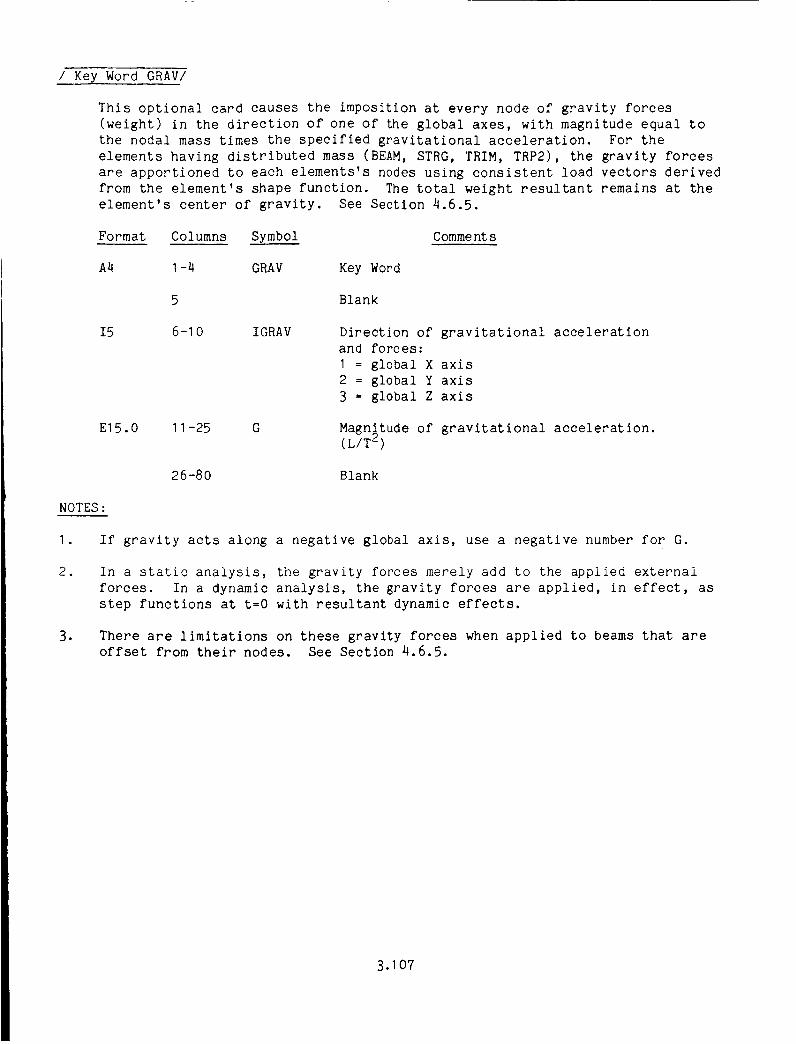
/ Key Word GRAV/

This optional card causes the imposition at every node of gravity forces

(weight) in the direction of one of the global axes, with magnitude equal to

the nodal mass times the specified gravitational acceleration. For the

elements having distributed mass (BEAM, STRG, TRIM, TRP2), the gravity forces

are apportioned to each elements's nodes using consistent load vectors derived

from the element's shape function. The total weight resultant remains at the

element's center of gravity. See Section 4.6.5.

Format Columns Symbol Comments

A4 I-4 GRAV Key Word

5 Blank

I5 6-I 0 IGRAV Direction of gravitational acceleration

and forces:

I = global X axis

2 = global Y axis

3 = global Z axis

El5.0 11 -25 G Magnitude of gravitational acceleration.(L/T _)

26-80 Blank

NOTES:

I. If gravity acts along a negative global axis, use a negative number for G.

. In a static analysis, the gravity forces merely add to the applied external

forces. In a dynamic analysis, the gravity forces are applied, in effect, as

step functions at t=O with resultant dynamic effects.

. There are limitations on these gravity forces when applied to beams that are

offset from their nodes. See Section 4.6.5.

3.107

/ Key Word ACELT/

This set of at least three cards is required whenever an applied displacement

ACEL is specified in Group E, p. 3.48. This card set defines an acceleration

versus time function to be assigned to specified degrees-of-freedom of

specified nodes by means of an identity number which appears here as well as in

the ACEL input. See Section 4.6.6.

Card I:

Format Columns Symbol

A5 I-5 ACELT

I5 6-15 ACELID

E15.0 11-25 NPT

E15.0 26-40 ODISP

E15.0 41-55 OVEL

56-8O

Comments

Key word

Identity number of this table

Number of points in the table, from 2 to 50.

Initial displacement (L).

Initial velocity (L/T).

Blank

NOTES:

(continued on next page)

3.108

/ Key Word ACELT/ Continued from previous page

This is followed by the number of cards equal to the value of NPT given in card

I, each card containing one point on the acceleration vs. time curve. The

first card must contain the initial time t=O, and the time must increase

monotonically with the following cards•

Cards 2:

Format Columns Symbol

A5 I-5 ACELT

6-10

E15.0 11-25 AC

El 5.0 26-40 TIME

41 -80

Comments

Key word, optional here.

Blank

Valu_ of acceleration at following time(L/T_).

Time (T).

Blank

NOTES:

I •

.

The applicable nodes and DOF are specified on the associated ACEL cards (p.

3.43 in Group E) bearing the identity number of this table•

For the special case of constant acceleration for all time, it is permitted to

use only one of these cards containing t=O and the desired constant

acceleration value• All other cases must use at least two cards.

• When the time exceeds the last time value specified here, the acceleration will

be held constant at the last value.

• A maximum of 36 time functions are allowed for the combined total of PTME,

PTM2, PTM3, and ACEL sets.

3.109

/ Key Word SEND/

This card ends the Group I data, and is required _ this group is used.

Format Columns Symbol Comments

A4 I-4 SEND Key word

5-80 Blank

NOTES:

3.110

/ Key Word STOP or END/

This is the required last card in the input deck. If END is used, the program

assumes that a new problem data deck will follow starting with the title card,

p. 3.1. If STOP is used, as will probably be the case for most problems, there

is no further data in the DYCAST input.

Format Columns Symbol Comments

A4 I-4 Key word STOP or END

5-80 Blank

3.111

4.0 INPUTREFERENCE

4.1 CONTROLPARAMETERSANDOPTIONS- GROUPA

4.1.1 Diagnostic Output (DYNA)

A provision has been madefor the user to request certain diagnostic output notusually needed. The current options are to print:

o Load vector

o Element stiffness and mass matrices (globally oriented)

o Coefficient matrix entries and stacking indices for each element.

o Assembled coefficient matrix

This output is triggered by the NPNTC input on the first DYNA card of Group A asfollows:

A I in column 7 prints the load vector, I in column 8 prints the element mass

and stiffness matrices, I in column 9 prints coefficient matrix entries with

their stacking indices, and a I in column 10 prints the assembled coefficientmatrix.

The first two items are printed only for t = O, while the last two will appear at

every time step.

Also on this card are input data that determines how often in time steps the

results are printed (NPRNT) and how often the coefficient matrix is reformed

(NFORM). If NFORM is zero the matrix is only assembled at the initial step. If an

implicit time integrator is selected in Group A (NEWM, WLSN, STAT), then NFORM is

ignored and it is internally set to I.

Example:

Print all four diagnostic output options. Print all results every 10 time steps

and reform the mass matrix every 1000 time steps.

0 ........ I......... 2 ......... 3 ......... 4 ......... 5 ......... 6 ......... 7 ......... 8

123456789_123456789_123456789_123456789_123456789_123456789_123456789_123456789_

DYNA 1111 10 1000

4.1

Examples of intermediate output generated with each option are shown below:

Load Vector

LOAD YECTOII DUE 1'0 JdPPL][E]D LOAD

ORIGINP, L _:_::- iS

OF POOR QUALITY

"°°"°°""' ,,o-ooo -.o ,,.o-o.-. i: oI.OooooooE+eO |.o0ooo0o£*ee |.oeooooo£,-H

17 I.ooooooo£-oo I.ooooOOOE*Oe I.llo000eE_li I.HOoOOO[.N I.lo00000[*eO I.IOOOOOO£*N |.NOOOOO[*H I.lOc:o00[,_l _2S e.eoooooe[.ee I.ooooooo£+qs| |.OeOOOOOE*M 0.800oo00[*U I.OoooOOOE_e I.DoeooooE,-ee I.eoo_ooo[-ee |.eoooooo£+-eo 3233 |.eoooooos.,.eo e.eoooooe£...ee e.eeooeeeE-ee e.HeoooeE..ee o.eoeeoooP,.H e.I)eooooes...ee o.eeoooeoi.ee e.eeooooo£.ee *e41 O.0O000DOE*IHD o.ooeooe0£+l_ O.Oo0o0eeE,.H I.OOOOOOOE.,.iN) o,eoeeoeo£...ee o.eeoooee£...oo o.ooeoooOE...oe o.l_oooo£.,,ee 4449 0.000DOD0£*00 0.000_000£.*.00 0.0o_0000E.qlO 1.1000000£*00 |.0000000£.,.e0 0.O0e0000E*00 0.0000000£*.1)0 0.D0;_000S.q)e 5657 0.0000000£*00 e.oo00000£*oo 0.0000000E*tI0 0.0e00000£*l_ 0.00000H£*H 0.lsOO0e00£,,-l)e o.ooooooe[*oe o.oeooooe£-,.eo _465 o.oooooDo[*oo 0.1)000000£*00 O.00O0000£*H |.OO00D00£,*.(10 0.0000D00E_-e0 0.0O00000£.*.e0 0.0O0O000E*60 0.OOO0000£-.e0 7273 o.ooooooo£-ee I.oooo+oot...oe l.eeeoooeE_-ee o.oooooooE+oe o.oooooeo['*'_o |.ooooooo[*oo I.+OOO0OCE-N 0.oo+o0_OE+ee GO81 I.oc0oooo£*eo O.o000_oo£+i_ o.oo000OOE.q)e O.i_)O0OO0E_.t)e O.0000oO0£.*'e0 |.O00000OE._.O0 |.OO000OOEolle |.000000O£.*./NI 18

The indices correspond to the degree-of-freedom. The first index for numbers

appearing on a line is in the left-most column and the last index in the right-most

co lumn.

Element Mass and Stiffness Matrices

EL[MERT IttSS KtTRZX FOR XEM_EIt 1

II. 0000O00£"e0 il. I)eooooo ['*'llo e.i)eooool)£*eoo.i_oooo_o¢.._._o 9.G2030_£"_| 1._k6_S_3E-_5 6.239323_E"_ i).i)00O00OE+Oe il.000O000E*'0eO.000O0O0E'.'0O 1.2796_8,0E"e_ k.239323flE-e6 1.1861716E-03 il.i)00ODI)0E'.'e0 il.i)_l)000(_E'.4)e

-1.'_t,'_'/61E-'i_. 0.O000000£*0e IJ.llooeooo£*._o 0.oo0000OE*e_ 2.4.&2820S£-03 -4..6S36,.11S£-.._-7.1_9_)831E--_ il.OODODOO[*i_ 0.i)_0OOO0£'*'i)O il.I)OO0OOOE'*'ee --4.653(_*,85E"1_ 3.3950323E-13

ELENENT STIFFNESS N&TR_X FOR N[NSER ]

COLUNNS I-4

1.9432927E+I)4 o.ooo;)ooes,.eo i).il000001_E*.l)e 0.i)el)0OeeE.-N -4,.9327730[+O7 -2.4050336["_II.lli_O0000_+l)O 1.30f19335E*l)4 -_.2862522£"04 1._)7311_,')2E*i_b O.IH)O_OOOE'*'eO I_.OO00000£_'l)OQ.OOOODOOE+O0 '-_.2BO2flZ2£*Ok 1.4)R31611_E+06 ')._2013'+_£",'ek O.O00_OOE*Ol_ 0.OOO_()OOE*0eO.O00OOOOE'*Oe 1.9731_12£'_B6 9.62_13_k£'-04 _.k256257£,'e7 II.OOOlP_OOE',,t_O II.ooooooo£,,.ee

-a_.93277311E-HI7 II.I)OBOOSB£*OI) O.I)0OO000£.*.(H! il.I)eOooo0£-.tH_ |.652S318£+e9 7.9",I15267E'417-2.41)50336E_II0 l. O0_00Oe£*i)_ il.l_,O00DC['*'l)0 i_.i)_Og_00E','_i_ 7.9485267£_-e7 2.GI_8135£'+I_7

This example is for a stringer element, which has three DOF for each. of two

nodes, thus a total of six DOF. These values are already transformed into the gl_ _l

directions.

Coefficient Matrix Entries to be Stacked with Their Stacking Indices

ELEM£NT MASS HATRZX ENTRZES TO |E ST_CXED, M_TH THEZR ST&CXZNG |NOZCES, FOR NEHBER I

_762 2.21180&OE--_ 4e9_1 Z.?k_299?E--_ 41219 1.62_31_9E-48 41220 _.5_|45_3[--_ &l&_? 1.279ktBOE-e& 41b&| 6.2393235E-.41&41_*_ 1.186_7_6£-03 4167_ -1._6_761E--_4 &1678 2._2828flE-_3 _1902 -7,149_832£-I_ _19_6 --_.6536,85[-H_ *19_7 3.395_323[--_3k0?57 1.*el?_13E--e6 4166_ --_.37_73_7E--_ &18)7 -_.61&SkS2£--B6 3_617 2.211806_E--e_ _egB6 --9.62B375fiE--e8 _121_ 7.B352332£-__1_2 3.$292248£-e6 398_6 1.56S_Sk3E-.e_ t_987 -¥.238fl12_£-0S _1215 -3.5292248£,.-I_ &1._3 -8.6350154E-O,,k, ,kO07_ -.i,.2393235E-e4,• 007_ 1.1861716E--_3 40760 _.3707307[-t_ 41672 -1.170278_£--_3 k190_ -|.3987811[--e4 _e301 1._6k_TkZE,-e4 _03_4 2._,,_282_5E-e3• 0761 _.klBSb52E-16 41673 -1.3987811|-_ _19|1 1.691S382E-t_3 _29 7.1_99831E,-_ 44Dfl32 -k.k536_SE--_ 44S33 3.3950323£-113

This is the contribution of the element t_ the global left-hand side coeffic_cnt

matrix, which, for explicit time integrators will be the mass matrix, and for implicit

integrators will be a combination of the stiffness and mass matrices (except at t _ 0

when only the mass matrix is used).

4.2

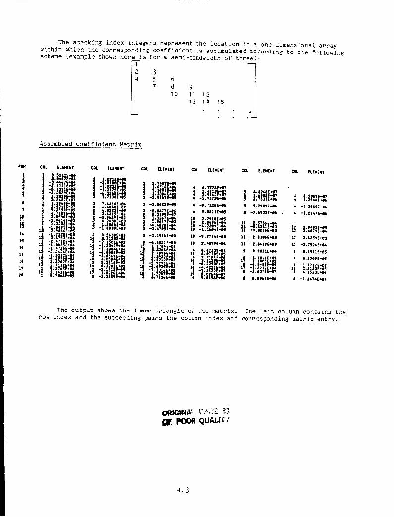
The stacking index integers represent the location in a one dimensional array

within which the corresponding coefficient is accumulated according to the following

scheme (example shown here is for a semi-bandwidth of three :mI

2

4 68I0

9

11 12

13 14 15

o

• q

Assembled Coefficient Matrix

_OW

12:14567

8

9

11111213

14

16

1.7

1!

19

2O

COL ELEMENT COL [LEI4ENT COL ELEHENT COL ELEMENT COL ELEMENT COL ELEMENT

t 3.5212E'_!_

3.1462E'.e4 i !.0218E+(I_

-3._,67E.04 -Z.oIooE.,._ S _.?447E*4H-2.1131E-45 -1.9338E+e_ 1.6S)6E*06 4 4.7'778E*417-.5.1391E*4_ -I.2175E*eS | 4 1.4213E...OT _.2268E..._

7.1591E_-2.2889E+06

3.8&87E-'47 -1.9167E'ql_ _ 1.6988£'.4T 6 8.f359E*tl?-1.9373E*416 2.7833E..06 6 1.39*_£,.06

1.3965£-l_ 2 ?.6416E.b06 $ 38_82E'04_ 4 -S.TZ26EqN; S f.29etE,.l_ 6 -2.2585_*_3. 924_E.qD7 8 4.4068 E'bO75._153£*e5 Z 4.0123E+4S 3 -2.i_??EH_ 6 9.1811E*4S S -7.6921E,_06 • 6 -Z.2747E,,464.7109E_06 6 3.6315E+06 9 8.21_9E÷17

I 2.|_96E_3 4.2438E*'e3 3 1.9697E'e3 10 2.$696E+I4 11-2.9689E-02 $ |.3267E'qJ4 11 2.?918E*e5

1 -2.e6)_E.e21.32e2t.q_ z_ |.eSe6E.t13 2.S?_5E.0.4_

1t -l.8*_lE',e4 l -1.613eE.,.03 I -Z._705E*/_"_'4828E't_ 10102.9866E*l_ 11 .._. 801_E*43 12 2. _il?gE*ll_I -1.7128E*_3 2 3.S638E_3 3 -2.2946E+43 10 --9.7714E_tl3 11 ,"2.8306E443 12 _.E359E,tO3

13 3.I7S3E46 14 3.112SE*O&-2._710E-04 2 -2.15_1£-43 $ "_._021E_.03 11 2.6g?gE*4_ 11 2.8_19E_l$ 12 -3.TS24E+_4-,_.eaes£*e4 14 -1.23_1£÷04 1_ ;.976_E_

Zx -1.6?26E-e5 2 -1.3BB_E*O6 a 3.3268E.,.4_ 4 6.6712E*e& S t.gI31E.H_ 6 1.6Sl1E,..1_13 -2.2_26£.'.4_ 1_ -,6.Se86E.,.03 S _.Te96£.q)4 16 4._718E_! 1.3_22E_-e3 _ 3.315_[.1_5 S 1.114_E*t_ k _.2SOSE,.eS:, .-,._e,e.e_ :* _._8,S-. :S *.,=:2e..*] :* _.::2e_,,-*,, :T 1.1e05£,-_

3.3262[_i_ , 2 8.3_1&E*E3 3 -_.99_SE*e4 4 .-6.28S_E*i_ --e.o_8_ E*eS2.7112E_ 14 6.3202E+_3 IS -_._3_E,_e4 16 -_._221E,-_ 1_ -1.8222E+14 18 2.813BE,*.IS1_ 9.22_5E*04

1_r -2.1418E*e_ 3 -7.3316E*B5 _ -1.2822E+47 S -2.I378E-47 6 _.1523E,_6t.1226E*e4 18 1.726TE*I_ 1_ S.I2_4E_0?11 S.TSk6E_l_ _ -1.21_9E,4_ • 3.773&E,,li_ 4 9.|LSIEe/N_ S 8.8f_lE_J6 6 -1.2474E-47

The output shows the lower triangle of the matrix. The left column contains the

row index and the succeeding pairs the column index and corresponding matrix entry.

_.3

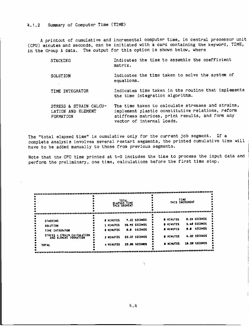
4. I. 2 Summary of Computer Tlme (TIME)

A printout of cumulative and incremental computer time, in central precessor unit

(CPU) minutes and seconds, can be initiated with a card containing the keyword, TIME,

in the Group A data. The output for this option is shown below, where

STACKING Indicates the time to assemble the coefficient

matrix.

SOLUTION Indicates the time taken to solve the system of

equations.

TIME INTEGRATOR Indicates time taken in the routine that implements

the time integration algorithm.

STRESS & STRAIN CALCU-

LATION AND ELEMENT

FORMATION

The time taken to calculate stresses andstrains,

implement plastic constitutive relations, reform

stiffness matrices, print results, and form any

vector of internal loads.

The "total elapsed time" is cumulative only for the current job segment. If a

complete analysis involves several restart segments, the printed cumulative time will

have to be added manually to those from previous segments.

Note that the CPU time printed at t=O includes the time to process the input data and

perform the preliminary, one time, calculations before the first time step.

i..............i .....iiiiiiiiiiil-i .......i: SOLLYT;ON * 1N|NUTES 33.9S SECONDS • O N|NUTES 3.60 SECONO$ :

,,,E,N,EO,.TO, : ,,,N_,S ,., SECONDS: , ,1N_ES,., SECO'DSi• STRESS _ STRAXN CALCULATION • • •• AND ELEH£NT FOR½ATION • 2 HINtJTES 22.37 SECONDS • 0 NINUTES G.32 SECONDS •

: : : :m TOTAL m 6 HIIlVTE$ 22.18 SECONDS • e HIHUTES 11.20 SECONDS •

4.4

4.1.3 Error Bounds for Modified Adams (ADAM)

The Modified Adams time integration procedure is based on the use of predicted

and corrected values for displacement and velocity. An error check on these quan-

tities determines whether quantities at the current time step have converged. Two

error terms that directly control convergence are read as Group A data on the card

containing the keyword ADAM. The parameter, EPSIL, is the upper bound error that

limits the size of the time step and the second, DELTA, is a lower bound error that

prevents the program from seeking time steps that are too small for the desired

accuracy. If the error exceeds the upper bound then the time step is halved; if the

error is less than the lower bound the time step is doubled. In practice, the upper

bound should be at least twice the lower bound in order to prevent excessive halving

and doubling.

If the error bounds are not specified then defaults of 10%, I% are taken.

A last parameter (ERR) on the card is essentially a tolerance that eliminates the

possibility that rou_doff errors will effect the convergence. The default for thisquantity is I. x 10 7.

Example: 15% upper bound, 5% lower bound

0 ........ I......... 2......... 3 ......... 4......... 5 ......... 6 ......... 7......... 8

123456789_123456789_123456789_123456789_123456789_123456789_123456789_123456789_

ADAM 0.15 0.05

4.5

4.1.4 Restart (REST)

The restart capability has been designed with a two-fold purpose: to restart ananalysis and to postprocess results of the analysis. To accomplish this, an externaldata base or "restart" file is created and manipulated by the program, with usercontrol by the RESTcard. First, initial information (model geometry, materialproperties, etc.) is written on this restart file after the input is processed. Then,a basic set of data consisting only of displacements, velocities, and accelerationsare saved on this file at each time step for postprocessing purposes. In addition, acomplete set of data (including stresses, strains, forces, etc.) are written at timestep intervals IPRNT, at which points the analysis can be restarted. The restart database file can be stored on any of the user's computer system storage media; forexample, tape or disk.

Wheninitially starting the analysis, the restart file is generated by settingIREST = 1.0 and specifying values for IPRNT and KPRINT (NUTAP and NRSRT are

ignored). If the entire REST card is omitted, then no restart file is created and no

restarts can be made, nor will there be any output data file for post-processing.

When restarting an analysis, IREST = 2 or 3. The two options differ only in that

IREST - 2 copies the current restart file before adding to it while IREST = 3 adds new

data directly to the existing file. The parameter NUTAP indicates whether the restart

file is to be continued, where NUTAP = 0 denotes that no further data is written and

NUTAP > 0 denotes that data will continue to be written on the file. The parameter

NRSRT, indicates the time step from which the continuation run will be re-started.

NRSRT is the time step number printed with an associated time during the run that

generated the restart file. IPRNT is again specified, and can be charged on a

restart.

The four IREST options 0,1,2,3 will usually require some differences in the Job

Control Logic (JCL) for the user's computer system, to access or not access the

external files.

Example I :

An initial restart file is to be generated, with full restart data every ten time

steps, and basic output data every step.

0 ........ I......... 2 ......... 3 ......... 4 ......... 5 ......... 6 ......... 7 ......... 8

12345678901234567890123456789012345678901234567890123456789012345678901234567890

REST I.0 I0.0

4.6

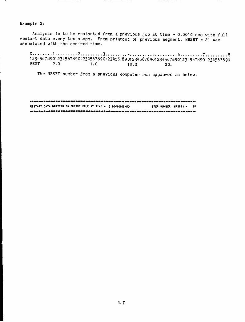
Example 2:

Analysis is to be restarted from a previous job at time = 0.0010 sec with full

restart data every ten steps. From printout of previous segment, NRSRT = 21 wasassociated with the desired time.

0 ........ I......... 2 ......... 3 ......... 4 ......... 5 ......... 6 ......... 7 ......... 8

123456789_123456789_123456789_123456789_123456789_123456789_123456789_123456789_

REST 2.0 1.0 10.0 20.

The NRSRT number from a previous computer run appeared as below.

4.7

4.1.5 Static Analysis (STAT)

A static analysis can be performed by specifying the keyword STAT in group A

data. This keyword has the effect of suppressing the mass contribution in the

equations of motion so that the following incremental equation is solved;

Kn AUn+I _ Pn+1 - fn (4.1 .I)

where K n

Pn+1

fn

AUn+I

is the incremental stiffness matrix

is the applied load vector

is the vector of internal forces at the start of the load step

is the displacement increment

All the input for a dynamic analysis is used in a static analysis with the exception

of initial conditions and lumped masses, Groups F and G input respectively.

The maximum load and load increment are controlled by specifying the maximum time

and time step on the second DYNA card in Group A input. This is used with the table

of load factor versus time, input with the keyword PTME in Group I data. This table is

a necessary input with a static analysis. (See Section 4.6.4). The time is used only

as a parameter to generate the loads.

The current load level or load increment is obtained from the table by inter

polating between any of the input values. One segment can be input if a constant load

step procedure is to be used. A variable step procedure can be defined by inputting a

number of segments. In this way, for example, large load steps can be taken at lower

load levels and smaller steps at higher !oadings where the problem nonlinearities may

require smaller time steps. The load (time) steps will be further varied, in any

case, by the convergence test.

4.8

4.1.6 Eigenvalue/Eigenvector Extraction (EIGN)

DYCAST implements an efficient algorithm for determining eigenvalues and

eigenvectors of large symmetric matrices. Specifically it implements an existing

program called ALARM (Automatic Large Reduction of Matrices to _ridiagonal form).ALARM is based upon an--algorlthm--prese_ted by Ojalv_and Newman which reduces a large

matrix to an "equivalent" trldiagonal form of much smaller size. It is similar to the

eigensolver FEER, which has been implemented in recent versions of NASTRAN.

The strength of the algorithm implemented in ALARM lies in the ability to per-

form the reduction in such a manner as to obtain the eigenvalues at either end of the

original matrix spectrum. In DYCAST this selectivity leads to accurate calculation of

the lower frequencies and modes. The size of the reduced matrix is usually

approximately 1.5 times the number of desired modes. The number of modes is specified

on the EIGN card by the parameter IQ. Internal error checking may increase the orderof the reduced matrix until it is rich in the lower modes that are desired.

Fundamental to the algorithm is a method that enforces each successive column of the

reduction matrix to be orthogonal to all other columns by an iterative method.

Experience has indicated that no more than two iterations are necessary for

convergence. The number of iterations is specified on the EIGN card as NSBAR.

The algorithm requires the stiffness matrix to be nonsingular. In the event that

the stiffness matrix is singular, a shift in [K] by some small amount will be required

in order to perform a matrix factorization, i.e.,

[K] + e[M] --[K] = [L][L] t.

The term, ¢, appears as EPS in the fifth field of the EIGN card.

(4.1.2)

* For full details of the method the reader is referred to "ALARM" - A Highly

Efficient Eigenvalue Extraction Routine for Very Large Matrices," by I. U. Ojalvo, The

Shock and Vibration Digest, Vol. 7, No. 12, December 1975.

4.9

4. I. 7 Automatic Element Failure (FAIL)

Material failure can occur when the principal strains equal or exceed the user-

specified failure strain values in both tension and compression. These failure

strains are input in the Group H material properties card sets (MBM, MSTG, MATI, MAT2,

MAT3). The failure criterion is applied to each stress integration point within an

element, provided that a non-zero tension failure strain is specified for that

element. If the tension failure strain is not specified for an element, then failure

of that element cannot occur and its material will have infinite strain capacity.

In the case of beam and stringer elements (MBM and MSTG inputs), only the

longitudinal strains are monitored and compared to the failure strains. For the

biaxially strained isotropic membrane and plate elements (MATI input), the in-plane

principal strains are calculated and compared to the failure strains. In the case of

the orthotropic biaxially strained elements (MAT2 and MAT3 inputs), the failure

strains vary with direction within the material. The user is required to specify the

failure strains in the material's directions of in-plane orthotropy, and the program

assumes a smooth elliptical variation with angle between these two orthogonal

directions. The in-plane principal strains are then compared to the failure strains

in the directions of the principal strains. The failure of nonlinear springs is based

on User-specified maximum values (+ and -) of elongation or rotation.

When an integration point fails, the values of stress and stiffness assigned to

the finite amount of material surrounding that point are set to zero, and its strain

energy is fixed at the current value, thereby becoming totally nonrecoverable. Thus

it can be seen that an element having only one integration point, such as a stringer

or a membrane, will be suddenly and completely failed whenever its single integration

point satisfies the failure criteria. For the beams, when all the integration pofnts

at either end node have failed, then the entire beam is failed. A "partial failure"

of a beam element is defined as when at least one integration point has failed, but a

complete element failure has not occured. At present, the automatic failure feature

for plate elements is not operational.

In this way, a partial failure of a beam may progress through its cross-section,

steadily reducing its forces, moments, and stiffnesses. This progressive failure may

actually reach a stable state, without further failure, if the element is buried

within a redundant structure containing other load paths. Since the stiffness of the

partially failed element is reduced, its internal forces may transfer to the remaining

stiffer load paths, and further progression of the partial failure may cease.

Should the required conditions for complete failure be achieved in an element,

then all that element's forces, moments, and stiffnesses become zero. Its strain

energy is "frozen" at the previous value, with no subsequent changes. The portion of

the total strain energy that was elastic or recoverable, is now arbitrarily made

nonrecoverable. Thus the elastic strain energy contained within the failed element is

not released to the system to be converted to kinetic energy or redistributed. (In an

actual material, some of this elastic strain energy is recovered by the system.)

4.10

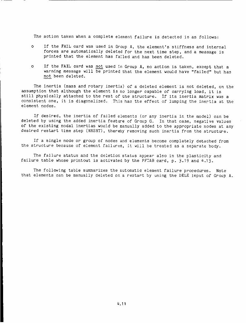
The action taken whena complete element failure is detected is as follows:

o If the FAIL card was used in GroupA, the element's stiffness and internalforces are automatically deleted for the next time step, and a messageisprinted that the element has failed and has been deleted.

o If the FAIL card wasnot used in Group A, no action is taken, except that awarning messagewill be printed that the element would have "failed" but hasnot been deleted.

The inertia (mass and rotary inertia) of a deleted element is not deleted, on theassumption that although the element is no longer capable of carrying load, it isstill physically attached to the rest of the structure. If its inertia matrix wasaconsistent one, it is diagonalized. This has the effect of lumping the inertia at theelement nodes.

If desired, the inertia of failed elements (or any inertia in the model) can bedeleted by using the added inertia feature of Group G. In that case, negative valuesof the existing nodal inertias would be manually added to the appropriate nodes at anydesired restart time step (NRSRT),thereby removing such inertia from the structure.

If a single node or group of nodes and elements becomecompletely detached fromthe structure because of element failures, it will be treated as a separate body.

The failure status and the deletion status appear also in the plasticity andfailure table whoseprintout is activated by the PFTABcard, p. 3.19 and 4.13.

The following table summarizes the automatic element failure procedures. Notethat elements can be manually deleted on a restart by using the DELEinput of Group A.

4.11

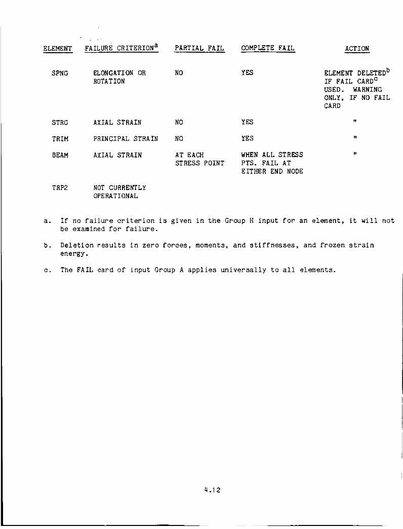
ELEMENT FAILURE CRITERION a PARTIAL FAIL COMPLETE FAIL ACTION

SPNG ELONGATION OR NO YES

ROTATION

STRG AXIAL STRAIN NO YES

TRIM PRINCIPAL STRAIN NO YES

BEAM AXIAL STRAIN AT EACH WHEN ALL STRESS

STRESS POINT PTS. FAIL AT

EITHER END NODE

TRP2 NOT CURRENTLY

OPERATIONAL

ELEMENT DELETED b

IF FAIL CARD c

USED. WARNING

ONLY, IF NO FAIL

CARD

a. If no failure criterion is given in the Group H input for an element, it will not

be examined for failure.

b. Deletion results in zero forces, moments, and stlffnesses, and frozen strain

energy.

c. The FAIL card of input Group A applies universally to all elements.

4.12

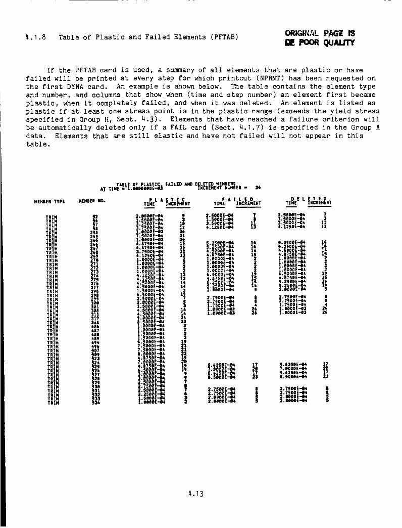
4.1.8 Table of Plastic and Failed Elements (PFTAB) ORIGiI_AL P./_'_ Is

Ol QuauTY

If the PFTAB card is used, a summary of all elements that are plastic or have

failed will be printed at every step for which printout (NPRNT) has been requested on

the first DYNA card. An example is shown below. The table contains the element type

and number, and columns that show when (time and step number) an element first became

plastic, when it completely failed, and when it was deleted. An element is listed as

plastic if at least one stress point is in the plastic range (exceeds the yield stress

specified in Group H, Sect. 4.3). Elements that have reached a failure criterion will

be automatically deleted only if a FAIL card (Sect. 4.1.7) is specified in the Group A

data. Elements that are still elastic and have not failed will not appear in this

table.

MEMBER TYPE

TRIMTRIMTRIMTRIMTRIMTRIMTRIMTRIMTRIMTRIMTRIMTRIMTRIMTR|MTRIMTRIMTRIMTRIMTRIMTRIMTRIMTRIMTRIMTRIMTRIMTRIMTRIMTRIMTRIMTRIMTRIMTRIMTRIMTRIMTRIMTRIMTRIMTRIMTRIMTR1MTRIMTRIMTRIMTRIMTRIMTRIMTRIMTRIM

TABLE OF PLASTIC. FAILED AND DELETED MEMBERSAT TIME s 1.UBDOOOE"II3 INCREMEMT NUMBER m IHb

MEMBER NO. P L A S T I C F A ; L E 0 D E L E T E D

tXM._!_X,CREMEM__TTm.._! I,CmEME_._-- tXM._2EI,CREME,T

2.,,,E-,, _ ,.,,,E-,,, t =.,,E-,, ;1. SOOeE.-I_ $ 1.5eOOE-e4 3 1.5000E443. 2500E-04 1B 3.5eDOE-e4 11 3.$000E-04 113.7SOOE-Ok 12 A. 1250E-I_ 13 4.12SOS-e4 131.0000E"03 2&7.5000E-'04 211.0000E-B3 2&4.8750E-06 15 _. 2500E"_ 1S 5.2_OOE-_ 164. 8750E-I)4 15 5.2500E"_ l& 5. 2500E-04 16

3.T,oe---- X2 ,.5oooE--,, :,, ,._,eS-.--+ |_,,.x2,e-e, x: ,.B_5o_-+, xS ,.at,e---+x.ooooe-.,, 2 I.eoooE-+, 2 1.oo.e-.o,x.ooooe-+, 2 1.,,--oE-,+ 2 X.eoooe-'_ |1.00ooe-e, 2 x.eeoeE--e, 2 1.00OOE--_1.eoOee.-e+ 2 X.e_OOE-*+ 2 :.®ooce.-e4 :_4.1250 E'e4 13 i. 5000E.-.04 19 6. 5000E-446.1250E'04 13 4. 6750 E-I_ 15 4. 8750E-Ok 15A. 5 OBOE-B4 l& 5.250C E-B4 16 _. 2500E,..0_ 16

4.5000E-04 14 5.2500E.-,04 lk 5.2590 E-.,04 1_1.50oo[ .-e,_ 3 2.00o0E-O* 5 2.00o0e--_6. 5000E-04 1_2. 5000E-04 • 2. ?500E-04 R 2. ?50BE-.04 !2. 0000E-e4 _ 2. 7500E--04 8 2.75DOE-B4 is1.5000E--04 3 1.7500E--04 A 1.7_00E-e&4.5000E-04 14 1 • 0000E-03 26 1. 0000E-03 2_

il 4. 5000E--4_, l& 1. i)000E-IB3 26 1. 0000E-'03 26

9. 0000E-04 24B.5000E-04 231. 0000E-06 21. eOOeE"04 21.5000E-I_ 21.5D(_OE-e4 36.5000E'-I_ 19?.SeOOE-e4 21?.50DOE-04 213. HODE"-04 224.8750E-'1_ 157. eOOeE.-IS_ 204.8750E-04 15 _. 6250E--04 IT |. 6250E--I_ 17

_26 6 • 5000E-'_ 19 T . IH_OOE-Ok 20 T. OOOOE,.-94 29

_27 3. eOeOE.-4_ 9 _. _250E.-4)4 17 S. 6250E.-0_ 1728 3. 000DE...4_ _ 8.5000 E-e4 23 B • 5000E-0_ 2329 2.5000E-I_ 7

r '31 2 • 5000E'-I_ ? 2 • ?_Be E..-I_ 8 2 • ?_E-I_32 2. 2500E-IUt 6 2. ?Sl_E-1_4 8 ,1 . T500E-l)4

1. 5000E'-t_ 3 3. 0000E-I_ S 2. _eeeE

4.13

4.1.9 Manual Deletion of Elements (DELE)

Any element can be manually deleted at the beginning of any restart segment.This can be used to simulate the failure of any structural element at somepoint inthe calculations. If it is desired to delete a group of elements, the key word DELEis specified in the Group A data along with a list of elements to be deleted. Once amanual deletion is specified on a restart, it is not necessary to repeat the deletionrequest for that element at subsequent restarts. However, it will probably beconvenient to repeat the previous deletions, and merely add the new ones to the end ofthe list.

Whenan element is deleted its stiffness contribution and internal force con-tribution to overall equilibrium is deleted from the equations of motion. The masscontribution, however, is maintained unless otherwise specified. Whenan element isdeleted, its masscontribution is no longer calculated from a consistent massmatrix,but rather by "lumping" proportional mass componentsat each node of the element.Inertia can be deleted for a group of deleted elements by specifying negative valuesof the existing inertia components to be added at the appropriate nodes at aconvenient restart time step (NRSRT). Since the inertia are additive, this actionwill remove such inertia from the structure.

4.14

4.1.10 Bandwidth Reduction (BAND)

Use of the optional BANDcard in Group A will cause a re-ordering of the Group Bnode list to reduce the bandwidth of the coefficient matrix, using an algorithmdevised by Collins*. This will reduce the core storage requirements and the computertime, and is essential for large problems.

The re-ordered node list will be printed with the processed input data, output onUnit 7 as a card image file for future use in the format required for the DYCASTGroupB input, and used directly in the current problem solution.

This re-ordering process includes the MPCspecifications as nodal connectivities,along with the elements.

After using BANDthe first time, the re-ordered nodal list from Unit 7 should beused to replace the original nodal list on subsequent runs, with the BANDcarddeleted. This process should be repeated whenever the connectivity of the model ischanged, especially for large problems.

The BANDoption previously used in the pre-processing program SATELLITE(Section 5) is also available, but is no longer supported.

*R.J. Collins, "Bandwidth Reduction By Automatic Renumbering" InternationalJournal for Numerical Methods In Engineering, Vol. 6, pp. 345-356, 1973.

4.15

4.2 GROUPB - NODESPECIFICATION

The Group B input defines an allowable set of external node point numbers. Theprogram uses this information in two ways. First, it sets up a table of allowable

node points that is used to check all subsequent node point input. Second, the

program converts each external node number to an internal number consecutively in the

order that the node appears on the input card. Consequently, the order of the input

of external node numbers i_ completely arbitrary and need not be increasing

monotonically. Once the input is read the program operates with the internal numbers

which are now numbered from I through the maximum number of nodes in the model. In

this manner the node ordering and therefore the bandwidth of the stiffness matrix can

be easily changed and nodes can be inserted or deleted by changing the external node

specification. A bandwidth optimizing subprogram is part of the input preprocessing

program SATELLITE. This program takes any order of external node number and prints a

reordered list of external node numbers which leads to an optimum bandwidth. (See

Section 5.1) Alternatively the BAND option, Group A data p. 3.24 can be used.

All the shorthand notation for fixed point input can be used with this input.

Example I:

Given a model with 100 nodes numbered consecutively, use shorthand notation:

0 ....... I ......... 2 ......... 3 ......... 4 ......... 5 ......... 6 ......... 7 ......... 8

12345678901234567890123456789012345678901234567890123456789012345678901234567890

1-100

Example 2:

Given a model with 100 nodes numbered consecutively I through 25, 31, 33, 34, 36,

50, 52, 54, ... 170

0 ....... I......... 2 ......... 3 ......... 4 ...... "...5 ......... 6 ......... 7 ......... 8

123456789_123456789_123456789_123456789_123456789_123456789_123456789_123456789_

I -25 31 33 35 36 50 -2 -170

Both shorthand notations are used, where 1-25 indicates I through 25, and 50-2-170

indicates 50 through 170 in increments of two.

4.16

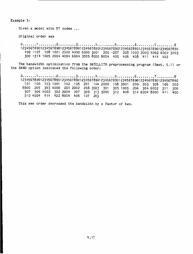
Example 3:

Given a model with 57 nodes ...

Original order was

0....... I ......... 2......... 3 ......... 4......... 5 ......... 6 ......... 7 ......... 8123456789_123456789_123456789_123456789_123456789_123456789_123456789_123456789_

100 -107 108 1001 2000 4000 6000 3001 200 -207 208 1003 2003 4002 6002 3003300 -314 1005 2004 4004 6004 3005 8000 8004 400 406 408 411 414 422

The bandwidth optimization from the SATELLITEpreprocessing program (Sect. 5.1) orthe BANDoption indicated the following order:

0....... I ......... 2......... 3......... 4......... 5 ......... 6 ......... 7......... 812345678901234567890123456789012345678901234567890123456789012345678901234567890

101 100 103 1001 102 105 201 104 2000 108 3001 200 203 308 106 2026000 205 303 4000 204 2002 208 3003 301 305 1005 206 304 6002 311 300307 306 4002 302 2004 207 309 313 3005 312 408 314 6004 8000 411 400310 4004 414 422 8004 406 107 203

This new order decreased the bandwidth by a factor of two.

4.17

4.3 ELEMENTPROPERTIES- GROUPSC ANDH

The theoretical basis of the elements are described in the DYCASTtheoreticalmanual. In this section a brief description of the theory is presented along with anexplanation of the input data cards necessary to use each element.

The topics discussed for each element include:

o

o

o

o

o

o

Introduction

Input Data

Element Connectivity

Material and Section Properties

Loads

Description of Output

4.18

4.3.1 Plasticity in General (MATI, MAT2,MAT3,MSTG,and MBM)

The methods used to implement plasticity theories into a finite element code bynow are well developed and have been reported in many references. The theoreticalbasis and the relevant equations that mathematically describe the plasticity theoryimplemented in DYCASTis described in Section I. This section outlines the form ofthe constitutive equations in a general wayand describes more fully the inputrequired to specify material properties.

DYCASTmakesuse of a flow theory of plasticity. Basic to this approach are thedefinitions of an initial yield criterion, and flow and hardening rules. The initialyield criterion used is based on Hill's equations for orthotropic material behaviorwhich reduces to the yon Mises yield criterion for an isotropic material. Use ofHill's equation requires the input of the yield stresses in the three principaldirections of orthotropy as well as a yield stress in shear. For an isotropicmaterial, this reduces to the specification of a single quantity, the yield stress,from a uniaxial tensile test.

From the flow and hardening rules the following incremental relation between theincrements of plastic strain and stress is obtained.

{aEp} = [c] {_o} (4.3.1)

where the terms of [C] are path dependent quantities that reflect the instantaneous

states of stress and hardening of the material and the choice of plasticity theory.

In DYCAST use is made of the Prager-Ziegler kinematic hardening theory. Also con

tained in [C] is a material parameter characterizing the hardening of the material.

In the one dimensional case this is represented by the slope of the stress versus

plastic strain curve. This is generalized to multiaxial stress conditions by assuming

an effective stress - effective plastic strain relation. Both linear and nonlinear

strain hardening options are available with input parameters determining which is

chosen. The Ramberg-Osgood three-parameter representation of the stress-strain data is

used for nonlinear hardening, where the plastic strain depends on a power of the

stress. This nonlinear relationship is written as

a 3g0.7 (______)n (4.3.2)c = _ * 7----_gO.7

Thus, for this representation of the stress strain curve, two additional material

parameters, n, gO 7' are required. To determine the values of n and gO 7 that best;fit the actual stress-strain data, the method suggested by Ramberg-Osgo6d

4.19

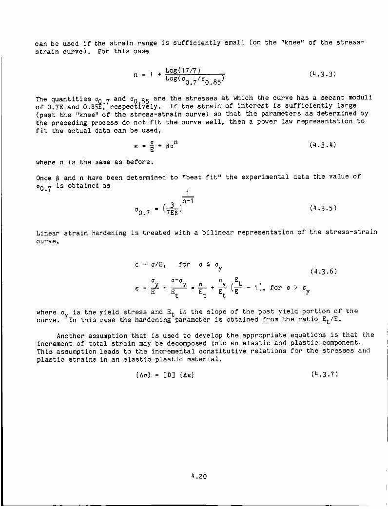
can be used if the strain range is sufficiently small (on the "knee" of the stress-

strain curve). For this case

n -- I + Log(17/7)

L°g(ao.7/aO.85)

(4.3.3)

The quantities a0 7 and a0 85 are the stresses at which the curve has a secant moduli

of 0.7E and O.85E_-respectively. If the strain of interest is sufficiently large

(past the "knee" of the stress-strain curve) so that the parameters as determined by

the preceding process do not fit the curve well, then a power law representation to

fit the actual data can be used,

o nc = - + Ba (4.3.4)

E

where n is the same as before.

Once 8 and n have been determined to "best fit" the experimental data the value of

aO. 7 is obtained asI

n-1

0.7 : (3) (4.3.5)

Linear strain hardening is treated with a bilinear representation of the stress-strain

curve,

c = a/E, for a < aY (4.3.6)

a a-a ay Etc ___ + y a + ( - I) for a > a

--E Et = E-_ E_t _-- ' Y

where ay is the yield stress and Et is the slope of the post yield portion of thecurve. In this case the hardening parameter is obtained from the ratio Et/E.

Another assumption that is used to develop the appropriate equations is that the

increment of total strain may be decomposed into an elastic and plastic component,

This assumption leads to the incremental constitutive relations for the stresses and

plastic strains in an elastic-plastic material.

--[D] {AE} (4.3.7)

4.20

and, from Eq (4.3.1),

{A_p} = [C][D] {AE} (4.3.8)

where Ae is the increment in total strain, [D] = [E-I + C]-I, and [E] contains theusual elastic material parameters.

Explicit forms for the relations in Eqs. (4.3.7) and (4.3.8) that are used inDYCASTare in Section 1.2. Equations similar in form to Eq (4.3.8) for perfectplasticity are also shown in that manual.

The following table lists the stress-strain curve types and the elements to whichthey apply. Tension and compression properties are assumedto be the same, except forfailure.

Material Yield MaterialKey Word Element Type, Elastic Criterion Type, Plastic

MATI TRIM Isotropic Isotropic,

TRP2 biaxialperfect plasticity,

linear strain

hardening, non-linear

strain hardening

MAT2 TRIM Orthotropic 0rthotropic

TRP2 biaxialperfect plasticity

MAT3 TRIM Orthotropic 0rthotropic

TRP2 biaxial

linear strain

hardening, nonlinear

strain hardening

MSTG STRG Isotropic Isotropic,

biaxial

perfect plasticity,

linear strain

hardening, non-

linear strain

hardening

MBM BEAM Isotropic Isotropic,

biaxial*

perfect plasticity,

linear strain

hardening, non-

linear strain

hardening

* Torsional shear included for solid and closed hollow cross-sections only, otherwise

uniaxial.

Cautionary Note:

In application, the linear elastic stress-strain curve, _ _ a/E, is followed

until the user-specified "yield stress" is exceeded. Then the program switches to Eq

(4.3.2). Therefore, the "yield stress" input for the Ramberg-Osgood nonlinear curve

should be equal to or less than the stress at which the nonlinear stress-strain cur_e

departs significantly from the elastic line. Otherwise, the nonlinear part of the

stress-strain curve will be incorrectly used by the program.

4.21

4.3.2 Stringer Element

4.3.2.1 Introduction

This element is used to represent a one dimensional axial force structuralmember. Twostringer elements are included: a two-node element developed from aconstant axial strain assumption and a three-node element developed from a linearlyvarying strain assumption (Fig. 4.3.1). As shown in Fig. 4.3.1, the indices i,jdenote the end point nodes of the two-node stringer and the indices i,j,k denote theend point and mid-length nodes of the three-node stringer. The specification of theaxial displacement componentu is sufficient to describe fully the elastic linearresponse of a stringer element since the element has no out-of-plane (normal to theaxial direction) stiffness. The normal components, v,w, contribute to the elasticgeometrically nonlinear response by coupling the axial force to the out-of-_lanedeformations This coupling leads to the initial stress stiffness matrix [k']. Itshould be noted that displacement components v, w, as shown in Fig. 4.3.1 refer toany two mutually perpendicular directions normal to the stringer axis since thestringer does not have a preferential cross sectional reference system.

L_ jj x,u

ZwW

j X,U

i_ y,v

Z,W

(A) CONSTANT STRAIN ELEMENT

Displacement Assumption

U = AI + A2X

(B) LINEAR STRAIN ELEMENT

Displacement Assumption

U = A I + A2X + A3X 2

Fig. 4.3.1 STRINGER

4.22

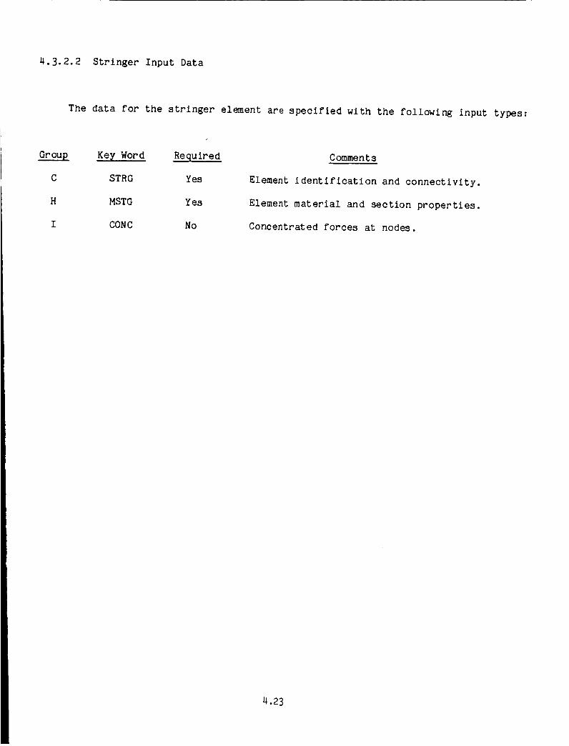
4.3.2.2 Stringer Input Data

The data for the stringer element are specified with the following input types:

Grou_ Key Word Required

C STRG Yes

H MSTG Yes

I CONC No

Comments

Element identification and connectivity.

Element material and section properties.

Concentrated forces at nodes.

4.23

4.3.2.3 Stringer Connectivity (STRG,Group C)

The nodes of the stringer element are specified with both major (end- point)nodes first, followed by the minor (midside) node. The absence of the midpoint nodemust be indicated by a zero o_ blank field in the proper position. The memberidentification can be any number of up to 5 digits. This number need not beconsecutive but must be unique for the job.

Example:

0........ I ......... 2......... 3......... 4......... 5 ......... 6......... 7......... 812345678901234567890123456789012345678901234567890123456789012345678901234567890STRG 5 I 2STRG 6 2 4 300

4.24

4.3.2.4 Stringer Material and Section Properties (MSTG,Group H)

The following material and section properties for the axial force stringer areinput:

E

A

PLASIPLAS2

YLDST

DENSITY

SEPST

SEPSC

Youngs's modulus

Cross-sectlonal area

See Table below

Yield stress (See Cautionary Note on p 4.21 )

Mass density (mass/unit volume)

Failure strain in tension (+)

Failure strain in compression (-)

Three types of plastic behavior can be considered, i.e., perfect plasticity,linear, or nonlinear strain hardening. They are indicated as follows:

Input ParametersPLASI PLAS2 Types of Plasticity

0 0 Perfect plasticity (zero slope in plastic range)

Et/E 0 Linear strain hardening, with E t equal to slope ofthe uniaxial stress versus strain curve in the

plastic range

n _0.7 Nonlinear strain hardening with Ramberg-Osgood

representation of the uniaxial stress-strain

curve, see p. 4.19.

Stringer material properties should be taken from curves of engineering stress

versus engineering strain. The engineering stress should be used because the program

multiplies it by the initial undeformed area (A) to get the resultant axial force.

The engineering strain should be used because the program converts it to true strain

internally (for stringer elements only). Tension and compression properties are

assumed to be the same, except for failure.

Note that, for ductile homogeneous materials, actual compression failures rarely

occur in the material. The first compression damage is usually from plastic shearing

or geometric instability (elastic or plastic buckling or collapse). In these cases,

the compression failure strain input can be made very large to prevent failure, or the

compression strain can be specified at which the actual damage is expected.

Instability can be more accurately determined by using beam and plate elements.

4.25

Example:

50 stringer elements, aluminum alloy

Area = .I in 2 for elements 1-25

Area = 0.15 in2 for elements 26-50

All material properties the same

Density = 0.1 ib/in 3 (2.588 x 10-4 ib sec2/in 4)

Young's Modulus = 10 x 106 psi

Yield = 36,000 psi

Linear strain hardening slope = 2 x 106 psi

No failure criterion for elements 1-25

Failure strain of 10%in tension and compression for elements 26-50

0........ I ......... 2 ......... 3 ......... 4......... 5......... 6......... 7......... 812345678901234567890123456789012345678901234567890123456789012345678901234567890MSTG I .0 E+07 0.1 0.2 O.

2.588 E-04 0.0 0.0I -25

MSTG 1.0 E+07 0.15 O.2 O.2.588 E-04 0.I -0.I

26 -50

36OOO.

36OOO.

4.26

4.3.2.5 Stringer Loads (Group I)

The following mechanical loads maybe applied to the stringer element:

CONC- Concentrated forces applied at specified nodes in the globaldirections in the units of force.

In addition, a table (PTME,or PTM2,or PTM3)of the load magnitude versus time,must be specified.

These loads are discussed in Section 4.6.

4.27

4.3.2.6 Description of Stringer Output

This section shows examples of typical output generated when using the stringer

element.

Stringer Connectivity

STRINGER ELEMENTSHEHBER NODE I NODE J NODE K

29 ]02 200030 2000 20231 202 200232 2002 30433 304 200434 2004 40835 4000 10636 296 400037 4002 20638 312 _00239 4004 31240 422 400475 1001 10176 201 190177 1003 20178 303 100379 1005 303BO 403 190581 105 300182 3801 20583 205 300384 3003 31185 311 300586 3005 411

In the absence of any three-node stringer elements, the third field for nodes

contains a blank. The midside external node number appears in that location when a

three-node stringer is specified.

4.28

Stringer Material Properties

YOUNG'S MODULUS3.8000000E+04

DENSITYB.80_88E+IM

APPLICABLE MEMBERS301 302 383

STRINGER SPECIFICATION TYPE 1AREA PLAS1 PLAS2 YIELD STRESS

1.0088800E-'04 O.00OOOOOE*OO 8.BBOOOBOE+O0 3.8080880E*84FAZLURE STRAIN

TENSION COMPRESSIONB.0008888E+00 B.8888800E+BB

This printout is generated when specifying stringer data with cards containingthe keyword MSTG.

Stringer Solution Output

The output shown below is for a two-node stringer since results for NODE K (the

mldside node) are blank. The nodal forces at each node are in the element axial

direction and AVERAGE STRAIN and EPS are the total and plastic strain, respectively.

The state of plasticity is indicated by the column labeled "PLASTIC". A "NO"

indicates an elastic element, "YES" indicates a plastic element, and "UNL" an element

that has unloaded elastically from a previously plastic state. Failed elements are

deleted from this output.

NODAL FORCES AND AVERAGE STRESS kRO $TRAZN FOR STRINGER HEMBERSA; TIME m 2.ODOBOOgE"03 ]NCREMENT NUI<BER - kO

NODAL NODAL NODAL AVERAGE AVERAGE AVERAGEMEMBER PLASTIC NODE | FORCE NODE J FORCE MOOEK FORCE $1RE$$ STRA|N PLAST]C STRA|_

301 NO 86 -6.B75&&SE".i_ 120 &.6786650-_ 6.&TE&ESE42 2.226222E-4_ |.O00000E*B&302 NO 120 2.T&42170-._ 11 -2.7642170-04 -2.764217E+00 --t.1473910-05 0.0000000*0_303 NO 120 -6.485425E--B* 9 -4.485425E-04 4.48562SE'_40 1.4951420-04 O.OOOOOOE*O&

4.29

4.3.3 BeamElement

4.3.3.1 Introduction

Somegeneral features and limitations of the beamelements are:

o Initially straight.

o Two nodes with 6 degrees of freedom per node.

o Constant cross-section along length.

O Thirteen pre-formed special cross-sections (L,T,C,etc.), with user specified

dimensions.

O Elastic geometric stiffness quantities (Area, moments of inertia) can be

either user-specified or calculated by the program. The torsional stiffness

constant must be input.

O Longitudinal, bending, and torsional deformations. No transverse shear

deformation.

O Interactive yield criterion involves combined normal and shear stresses due

to longitudinal forces, bending moments, and torsion for closed thin-walled

and solid cross-sections. The shear stresses due to torsion are neglected

for open thin-walled sections.

Each beam element must be homogenous (one material), but any number of beam

elements, each having its own material, can be combined into a beam assembly

that acts as a single beam between common end nodes.

cross-sections do not deform, however the reduced bending strength due to

distortions of hollow, thin-walled beams can be represented by a nonlinear

rotary spring having a user-specified curve of moment vs. rotation.

There are four sets of local axes used in the beam elements as follows (Figs

4.3.2 through 4.3.4):

O Nodal axes x,y,z - Defined by the nodes, and describe the general position of

the beam's initial rotational position about its longitudinal x axis, and is

defined by the "pointer" node (Fig 4.3.2). This is described in detail later

in Section 4.3.3.3.

4.30

o Cross-sectional axes x'y'z' - Fixed in the cross-sectlon, with origin at its

shear center. Usually coincident with the reference axis x"y"z" (default

condition) as shown in Fig. 4.3.2. Can be rotated and translated relative to

the reference axes as in Figs 4.3.3 and 4.3.4. The location of these axes

for each beam cross-section is given in Section 4.3.3.5.

Centroidal axes x y z - Parallel to the cross-sectional axes, but through

the centroid of area for the cross section.

Reference axes x"y"z" - Parallel to the nodal axes, with origin at the shear

center, relative to which the cross-sectional axes x'y'z' can be rotated and

translated in the transverse plane as in Figs 4.3.3 and 4.3.4. Fig 4.3.2

shows the (default) use of no rotation or translation. Used for changing the

rotational orientation of a beam from that defined by the nodal axes, or for

combining a number of separate beam elements (different materials allowed)

into an assembly that acts as a single beam. The origin of these reference

axes must be placed at the shear center of the combined beam assembly.

Note that the cross-sectional axes x'y'z' remain fixed in the cross-section and

rotate and translate with it. In the right side of Fig. 4.3.4, the other beam cross-

sections that form the combined beam are omitted. The reference axes x"y"z" are

centered at the shear center of the combined beam assembly and apply to all the beams

that are combined into the assembly, and serve to locate the relative positions of

these beams.

In actuality, the reference axes x"y"z" are always present, but are coincident

with the cross-sectional reference axes x'y'z' when yA--ZA=8=O in Figs 4.3.3 and4.3.4. Thus the user can ignore these input parameters and the reference axes until

they are needed. The procedure and examples for creating a combined beam assembly are

given in Section 4.3.3.5.

These local axes completely define the initial (undeformed) position of a beam

element in the structure. As the beam deforms, these axes move together relative to

the global coordinate system.

In the following discussion the terms "reference axes" and "shear center" pertain

to the cross-section reference axes and their associated shear center unless the new

reference axes are used.

4.31

(POINTER) NODE k

c! ;c_v

v'" yT SHEARCENTEF

Fig 4.3.2 Basic Axes For Beam Cross-Sections

y

Z

NODE _.__ Yo

Z ,0

Z Y"

i _ z'

Y" v SHEAR

V

NODE_ YO

y"

Z'

_A YA

Z Io

Y" NEW SHEAR

CENTER OF COMBINED

BEAM ASSEMBLY

Fig 4.3.3 Rotating a Beam

Cross-sectionFig 4.3.4 Rotating and Translating

a Beam Cross-Section as part of a

Combined Beam

4.32

The stiffness properties for an initially straight beamelement of arbitrarycross section are based on the assumptions of classical beamtheory. These assumptionsinclude:

I) Normals to the centroidal axis remain straight and normal after deformation

and their length remains unchanged, i.e., the effect of transverse shear

deformation and transverse normal strains are neglected.

2) Longitudinal warping of the cross section out-of-plane is neglected.

3) Transverse deformations within the cross-section are neglected, i.e., cross-

sections are rigid (no crippling of thin flanges or webs).

4) Isotropic material, for which G : E/2(I + v) is used in the elastic torsional

stiffness. (A special case of a transversely isotropic material is also

allowed. See discussion below.)

Although assumption 2) is restrictive for all but circular cross sections, the

ability to specify the actual elastic torsional rigidity has been maintained. The

basic beam coordinate systems are defined in Fig. 4.3.2. Note that the shear center

and centroid do not necessarily coincide, and that the node can be anywhere in the

plane. The reference axes at the shear center are parallel to the nodal axes. The

geometry is the same at both ends of the beam element. Based on the right-hand rule

for moments and rotations, and assumptions I) and 2) above, the displacements at any

point within the beam cross section can be written as

u = Ucg + (z' - Zcg) 8y - (Y' - Ycg) 8z

V = VSC - Z 8x

!

w -- Wsc + y 8x

(4.3.9)

where u is the axial displacement of the centroidal axis; Vsc, Wsc are the lateralcg

displacements of the shear center in the cross sectional y' and z' directions; 8x, By,

8z are the cross sectional rotations about the shear center; and Ycg' Zcg are thecoordinate distances from the shear center to the centroid.

There are four independent displacement components that are prescribed to

formulate the beam element stiffness properties. These are the two transverse

displacement components Vsc, Wsc and the axial displacement and twist _cg and 8x. Theout-of-plane rotations are related to the transverse displacements in one usual manner

by imposing Kirchoff's hypothesis, i.e.,

_y = -W,x , 8z = v, x (4.3.10)

The two components of transverse displacement are assumed to be cubic functions

that are solutions to the linear homogeneous beam equations while the axial

displacement and twist Ucg , 8x are linear functions of the axial coordinate.

4.33

In the completely elastic case, the beam stiffness matrix involves elasticmaterial properties and integrated quantities that depend on the cross-section, thearea, and momentsof inertia. Oncepoints on the beamare plastic, these quantitiesmust be numerically integrated. In order to accomplish this, it is necessary tolocate "integration points" within the element cross-section. Consequently, the shapeof the cross section must be input and the state of stress and strain evaluated ateach integration point. Thirteen distinct cross sections can currently bespecified. Theseshapes are discussed in Section 4.3.3.5 below.

Specifically, it is assumedthat plastic strains (and therefore plastic materialproperties) vary linearly between nodes and that the "integration points" are locatedat Gauss-Legendre integration points in the cross-section at either end. The numberand location of the Gausspoints for each cross-section are discussed in Section4.3.3.5 below.

An additional point to be madeis that the torsional shearing stresses areneglected in the yield function and the plastic constitutive relations for all thethin walled open sections. Becausewarping is neglected for the beamsections thenumerical integration can over-predict the torsional stiffness. Consequently, theseterms are reduced by a "knock down" factor which is the ratio of the input elastictorsional constant to the elastic torsional constant obtained whenwarping isneglected. Thus, the integrated plastic torsional stiffness is reduced by the samefactor that reduces the elastic torsional stiffness.

A transversely isotropic beamis also allowed, for which the transverse (yz)plane is isotropic, but the beamlength (x) direction is a principal axis oforthotropy. In that case, Ex is input for E, and the input value of Poisson's ratioshould be _ -- (Ex/2Gxz)-1 as a device to have the proper value of Gxz calculatedinternally, for use in the torsional stiffness. However, the isotropic yieldcriterion will still be applied, so that the plastic behavior of the material will bein error. If such a beamis madeof a very brittle material, having little or noplastic strain before failure, then the yield limitation does not apply. A commonexample of such a brittle elastic material is a resin reinforced by high stiffnessuniaxial continuous fibers, such as in a graphite fiber/epoxy resin system.

4.34

4.3.3.2 BeamInput Data

The data for the beamelement are specified with the following input types:

Group Keyword Required

C BEAM Yes

H MBM Yes

SREC Yes*

SCIR Yes*

HREC Yes*

HCIR Yes*

LSEC Yes*

TSEC Yes*

ISEC Yes*

ZSEC Yes*

ZSCR Yes*

CSEC Yes*

HSEC Yes*

TWD Yes*

LSEG Yes*

Comments

Element identification and

connectivity.

Beam material properties.

Solid rectangle.

Solid circular.

Hollow rectangular.

Hollow circular.

L - section.

T - section.

I - section.

Z - section.

Z-section reserved.

Channel - section.

Hat - section.

Planar section.

Thin Line Segment.

I BMLO No

CONC No

Linear varying distributed lateral

load on a beam element.

Concentrated forces and moments at

nodes.

*Each beam element must be identified with one of the cross sections listed. One

specification can be applicable for a number of elements having the same section

properties.

4.35

4.3.3.3 BeamConnectivity (BEAM,Group C)

The beamconnectivity card begins with the key work BEAM,followed by the beamelement number, followed by three node numbersdefining node i, node J, and node k insequence. The use of this three-node sequence is described in the followingdiscussion.

The beamelement initial position is described by three distinct node points.The nodal x-axis is defined from node i to node j (Fig. 4.3.2). The nodal y-axis isparallel to the perpendicular from the x-axis through the node k, and the nodal z-axisis perpendicular to the x-y plane. The node k (called the "pointer" node) is usedonly for the purpose of defining the initial orientation of the beamcross section,and can be an existing node in the structure or a node specified only for thispurpose. In the latter case, all degrees of freedom associated with that node must be

fixed. Once this additional point is defined, the direction cosine transformations

between the nodal and global directions are completely determined. The beam cross-

section geometry (shape and position) is specified relative to these nodal axes, as

described in general in Section 4.3.3.1 above, and for specific cross-sections in

Section 4.3.3.5 below.

0 ........ I......... 2 ......... 3 ......... 4 ......... 5 ......... 6 ......... 7 ......... 8

123456789_123456789_123456789_123456789_123456789_123456789_123456789_123456789_

BEAM 10 100 105 26

too

26

4.36

4.3.3.4 BeamMaterial Properties (MBM,GroupH)

The following beammaterial properties are input.

Young's modulus

- Poisson's ratio

- See Table below

E

ANU

PLASIPLAS2

YLDST

DENSITY

BEPST

BEPSF

Yield stress (See Cautionary Note p 4.21)

- Massdensity (mass/unit volume)

- Failure strain in tension (+)

- Failure strain in compression (-)

Three types of plastic behavior can be considered, perfect plasticity, linear, ornonlinear hardening. They are as follows:

Input ParametersPLASI PLAS2 Types of Plasticity

0.0 0.0 Perfect plasticity (zero slope in plastic range)

Et/E 0.0 Linear strain hardening with Et equal to the slopeof the uniaxial stress versus strain curve in the

plastic range

n aO. 7 Nonlinear strain hardening with Ramberg-Osgood

representation of a uniaxial stress-strain curve,

see p. 4.19.

Beam material property parameters should ideally be taken from curves of

engineering stress versus true strain. Engineering stress should be used because the

program does not alter the cross-section area due to Poisson's ratio under axial

strains. Using engineering strain will involve strain errors whose magnitude is

approximately half the strain (e.g., 10% strain gives an error of 5%), and in many

cases this error is acceptable. The material stiffness integrations will be effected

only for nonlinear hardening, because the tangent modulus in the plastic range are

constant for linear hardening and perfectly plastic materials. Stresses will not be

significantly affected by this strain error in the case of perfect plasticity.

Therefore, using engineering stress-strain curves should be adequate for most

purposes. Tension and compression properties are assumed to be the same, except for

failure.

4.37

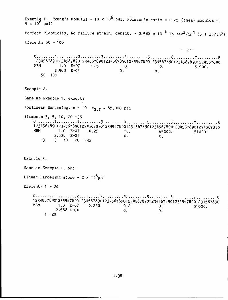
Exampl_ I. Young's Modulus _ 10 x 106 psi, Poisson's ratio -- 0.25 (shear modulus --4 x 10v psi)

Perfect Plasticity, No failure strain, density _ 2.588 x 10-4 ib sec2/in 4 (0.1 ib/in 3)

Elements 50 - 100

0........ I ......... 2......... 3 ......... 4......... 5 ......... 6 ......... 7......... 812345678901234567890123456789012345678901234567890123456789012345678901234567890MBM I .0 E+07 0.25 O. O. 51000.

2.588 E-04 O. O.50 -100

Example 2.

Sameas ExampleI, except:

Nonlinear Hardening, n -- 10, o0.7 z 65,000 psi

Elements 3, 5, I0, 20 -350........ I ......... 2......... 3......... 4......... 5 ......... 6 ......... 7 ......... 812345678901234567890123456789012345678901234567890123456789012345678901234567890MBM I .0 E+07 0.25 10. 65000. 51000.

2.588 E-04 O. O.3 5 10 20 -35

Example 3.

Sameas ExampleI, but:

Linear Hardening slope = 2 x 106psi

Elements I - 20

0........ I ......... 2 ......... 3......... 4......... 5 ......... 6......... 7 ......... 8123456789_123456789_123456789_123456789_123456789_123456789_123456789_123456789_MBM 1.0 E+07 0.250 0.2 O. 51000•

2.588 E-04 O. O.I -20

4.38

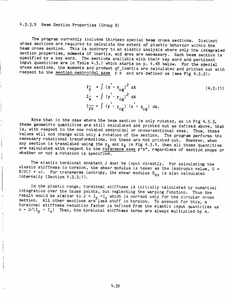
4.3.3.5 BeamSection Properties (Group H)

The program currently includes thirteen special beamcross sections. Distinctcross sections are required to calculate the extent of plastic behavior within thebeamcross section. This is contrary to an elastic analysis where only the integratedsection properties, momentsof inertia, and area are necessary. Each beam section isspecified by a key word. The sections available with their key word and pertinentinput quantities are in Table 4.3.1 which starts on p. 4.48 below. For the specialcross sections, the momentsand product of inertia are calculated and printed out withrespect to the section centroidal axes y z and are defined as (see Fig 4.3.2):

f ' Zcg) 2I_ = (z - dA

f ' Ycg) 2Ii = (y - dA

' Ycg ) 'Iy z (y (z Zcg) dA.

(4.3.11)

Note that in the case where the beam section is only rotated, as in Fig 4.3.3,

these geometric quantities are still calculated and printed out as defined above, that

is, with respect to the now rotated centroidal or cross-sectional axes. Thus, these

values will not change with only a rotation of the section. The program performs the

necessary rotational transformations, but these are not printed out. However, when

any section is translated using the YA and z A in Fig 4.3.4, then all these quantities

are calculated with respect to the reference axes y"z", regardless of section shape or

whether or not a rotation is specified.

The elastic torsional constant J must be input directly. For calculating the

elastic stiffness in torsion, the shear modulus is taken as the isotropic value, G =

E/2(I + v). For transverse isotropy, the shear modulus Gxz is also calculatedinternally (Section 4.3.3.1).

In the plastic range, torsional stiffness is initially calculated by numerical

integration over the Gauss points, but neglecting the warping function. Thus the

result would be similar to J -- Iy +I z which is correct only for the circular crosssection. All other sections are less stiff in torsion. To account for this, a

torsional stiffness reduction factor is defined from the elastic input quantities as

n -- J/(Iy + Iz) Then, the torsional stiffness terms are always multiplied by n.

4.39

The first card of this set begins with one of the beamsection key words andcontains the cross section properties. If area, momentsof inertia, and product ofinertia are all input as zero or blank, then these four quantities are calculatedinternally, based on the section dimensions, by numerical integration using the Gaussintegration points for the section (Table 4.3.1 starting on p. 4.48). The numericalintegration of momentsof inertia neglects the contribution of the momentof inertiaof a flange or webcomponent about an axis through its own centroid parallel to itslength. This contribution is usually very small for thin walled sections. Thus forthick flanges and webs, where this term is significant, the correct elastic values of

Izz, and Ivz should be input directly. This approximation results from using onlyoneIyY'integration-point across the thickness of flanges and webs and does not apply to

solid rectangular or circular cross sections. The input values of these quantities

are used only in the elastic range, while the integrated quantities are used in the

plastic range. Therefore, a thick-walled section is treated as a thin walled section

in the plastic range for calculating the stiffnesses.

If the moments of inertia are input they must be with respect to the proper axes

defined by Eq. (4.3.11) or (4.3.12) on p. 4.39 above.

The second card defines eccentricities, _, zo, an orientation angle, B, and twoquantities YA, ZA which define the placement a beam section relative to thereference axes at the shear center of a combined beam assembly (see Fig 4.3.4).

The nodal eccentricities Yo' Zo are the distances from the cross sectional shearcenter to the node (see Figs. 4.3.2 through 4.3.4). Eccentricit_e's ar_ _ s-ame

each end of the beam. The location of the shear center is shown in Table 4.3.1 for

each special section. Note that if a group of beam elements form a combined beam

assembly they will all have the same reference axes y"z" (Fig 4.3.4) and the same

nodes. Therefore the yo,Zo inputs will be the same for all beam sections forming the

assembly.

The parameters 8, YA' and zA (called BETA, YA, and ZA in the input) are used todefine a new set of reference axes y" z" for a beam element, as shown in Fig. 4.3.4.

Fig 4.3.3 shows the use of S alone to rotate a beam element from its originally

specified position. In that case, the cross-section and its axes y' z' are rotated

through an angle B relative to the stationary y" z" axes which remain parallel to the

nodal axes y z. The beam's cross-section stiffness and dimensions (input on the

first, third, and subsequent cards of this card set) are unchanged, since they remain

assigned to the y' z' axes that rotate with the cross-section. The nodal

eccentricities Yo Zo specified on card 2 of the set are also unchanged, since they arenow measured from the unmoved y", z" axes. Thus, a beam can be easily rotated about

its longitudinal axis to any angle from its original orientation by merely specifying

the desired angle B (BETA) on card 2 of the section property input set. The axes y"

z" become the new reference axes for the element. This feature can be applied to any

beam section, as a simpler alternative to moving its pointer node.

In the more general case, shown in Fig 4.3.4, a beam can be translated as well as

rotated relative to the new reference axes y" z". The nodal eccentricities Yo' Zo are

now specified relative to the new axes. This feature is used to combine two or more

separate beam elements into one single-actlng beam. Since each component beam element

can have its own material properties (MBM input), this is the way to create a multi

material beam model. The procedure is as follows:

4.40

I. Prepare a drawing of the combined cross-section.

2. Locate the node position and the orientation of the nodal axes y z using thepointer (k) node. See Fig 4.3.2.

3. Locate the shear center of the combined Cross-section and place the referenceaxes y" z" there, parallel to the nodal axes. Measure the nodal position (Yo'zo) from these reference axes.

4. Break up the combined cross-section into sub-sections, according to materialtype and geometry. Each sub-section must be capable of being defined by oneof the cross-sectlon geometries available in Table 4.3.1, and is to be given aseparate beamelement number.

5. Locate the position and orientation of each sub-section's axes y' z' as shownin Table 4.3.1 starting on p. 4.48. (See Fig 4.3.4 above and Example 4p. 4.46 below.) Measure the rotational and translational positions (8, YA,zA) of each sub-sectlon's y' z' axes from the new reference y" z" axes. Usethe right-hand rule for rotation about the beam's longitudinal (x) axis.

6. Prepare a separate BEAMconnectivity card (Group C input) for each sub-sectionbeam, having different beamnumbersbut identical node numbers.

7. Prepare an MBMmaterial properties card set (Group H input) for each separatematerial used in the combined section. Sub-sectlon beamshaving the samematerial can share one MBMset.

8. Prepare a geometric properties card set (Group H input, key words ISEC, TSEC,etc) for each sub-sectlon beam. Note that the nodal eccentricity (Yo' Zo) oncard 2 of this set is_the samefor all sub-sections of a combined beam.

The geometric stiffness quantities A, I , Iz, I.z, J will be printed out for eachsub-section beam, relative to the new refereYnoeaxesYy'' z", and represents each sub-section's contribution to the total section's value of these quantities.

4.41

The next card(s) contains cross section dimensions.4.3.1 and are listed below for each special cross section:

SREC A B Card 3

SCIR R Card 3

HCIR R T Card 3

HREC AI A2 TI T2 Card 3

LSEC AI A2 TI T2 Card 3

TSEC AI A2 TI T2 Card 3

ZSEC AI A2 A3 Card 3TI T2 T3 Card 4

ZSCR AI A2 A3 Card 3TI T2 T3 Card 4

ISEC AI A2 A3 Card 3TI T2 T3 Card 4

CSEC AI A2 A3 Card 3TI T2 T3 Card 4

HSEC B BI H T Card 3

TWD W T NLAY Card 3

LSEG YI ZI Y2 Z2 Card 3

T Card 4

These are tabulated in Table

4.42

The two dimensional beamsection, TWD,(Table 4.3.1) is used for a beamelementrestricted to deformation in the local x-z plane defined in Fig. 4.3.2. The input forthis section is the width, W, perpendicular to the plane of deformation, the thickness(depth), T, and the number of layers, NLAY,through the thickness. NLAYis used todefine Simpson's rule integration points at the boundary of the layers. Up to 58layers can be specified defining 59 integration points through the thickness. NLAYmust be an even number, from 2 to 58.

Example I.

Solid Rectangular Section z'

elements 18, 22, 68, 72, 73

0........ I ......... 2......... 3......... 4......... 5......... 6 ......... 7......... 8123456789_123456789_123456789_123456789_123456789_123456789_123456789_123456789_SREC 2.0 0.1667 0.6667 O. 0.458

O. O. O.2.0 1.0

18 22 68 72 73

4.43

Example 2.

L-Section

I

i

z' elements 29 - 40,

75-86

0.0625

0.0625

w

O ........ I ......... 2 ......... 3 ......... 4 ......... 5 ......... 6 ......... 7 ......... 8

123456789_123456789_123456789_123456789_123456789_123456789_123456789_123456789_

LREC 0.1211 0.01099 0.01099 -0.007087 1.6276 E-04

0.9375 0.9375 O.

1.0 1.0 0.0625 0.0625

29 -40 75 -86

Example 3.

I-Section

elements I - 100ml

12,

T14

±

T 1 "T2-T3- 1

0 ........ I ......... 2 ......... 3 ......... 4 ......... 5 ......... 6.........7.........8

123456789012345678901 2345678901234567890123456789012345678901234567890123456?890

ISEC 30. 855. 163. O. IO. 667O. O. 0.

6. 14. 12.

I. I. I.

I -100

4.45

Example 4.

Hollow Rectangular Section

Composedof two LSEC's combined, using the b, YA' ZA inputs.

NOTE: Two beammembercards must be specified in Group C data.dimensions are:

The L-sections

Section AI A2 TI T2I .95 .975 .025 .0252 .95 .975 .025 .025

The origin (mid thickness at the intersection) of Section I is placed at the lowerleft corner of the rectangle. The origin of section 2 is placed at the upper rightcorner and section 2 is rotated 180°.

Section 11

.g75

Section 2

"r yU

0 ........ I ......... 2 ......... 3 ......... 4......... 5 ......... 6 ......... 7 ......... 8

123456789_123456789_123456789_123456789_123456789_123456789_123456789_123456789_

LSEC (four blanks request internal calculation) .02317

O. O. O. -.475 -.475

.95 .975 0.025 0.025

I

LSEC (four blanks request internal calculation)

0.0 0.0 180. .475

.95 .975 0.025 0.025

.02317

.475

4.46

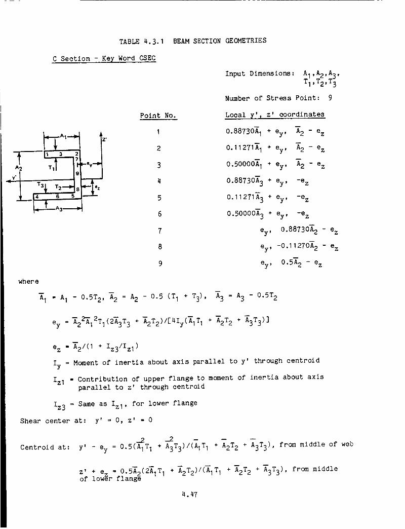
where

TABLE4.3.1

C Section - Key Word CSEC

• z

Point No.

I

2

3

4

5

6

7

8

9

BEAM SECTION GEOMETRIES

Input Dimensions: AI,A2,A3,

TI,T2,T 3

Number of Stress Point: 9

Local y', z' coordinates

0.88730A I + ey,

0.11271A I + ey,

0.5000_ I + ey,

0.88730_ 3 + ey,

0.11271A 3 + ey,

0.50000_ 3 + ey,

_2 - ez

_2 - ez

_2 - ez

-e z

-e z

-e z

ey, 0.88730_ 2 - ez

ey, -0.11270A 2 - e z

ey, 0.5_ 2 - ez

_I = AI - 0"5T2' _2 = A2 - 0.5 (TI + T3), _3 = A3 - 0"5T2

ey = _22-AA12T1(2_3T3 + A--2T2)/[4Iy(_ITI + _2T2 ÷ A3T3 )]

e z =_21(I + Iz3/Izl)

Iy = Moment of inertia about axis parallel to y' through centroid

Izl = Contribution of upper flange to moment of inertia about axisparallel to z' through centroid

Iz3 = Same as Izl, for lower flange

Shear center at: y' = 0, z' = 0

Centroid at:

...2 ..2 _ m

y' - ey = 0.5(AIT I + A3T3)/(AITI + A2T2 + A3T3), from middle of web

z' + e_ = 0.SA--_(2AIT I + A--2T2)/(_1T1 + A--2T2 + A%T3), from middleof lower flange

4.47

TABLE4.3.1 BEAMSECTIONGEOMETRIES(continued)

Hollow Circle - Key Word HCIR

Y' 4

Input Dimensions: R, T

Number of Stress Points: 12

Point No. Local r, e coordinates

I R, 10.14 o

2 R, 79.86 o

3 R, 45.00 °

Points in the second through fourth quadrants are

located by addlng 900 , 180 0, 2700 to the angles listed

above.

stress points

symmetric about y' where R = R - 0.5T

Origin at shear center

Centroid at origin: y' = O, z' = 0

4.48

TABLE4.3.1 BEAMSECTIONGEOMETRIES(continued)

Hollow Rectangle - Key Word HREC

y'_

Z"

t3 2

110

12

T1 T 2

_r ill

4 6 5

-_ A 1

Input Dimensions: A I,A2,TIT 2

Number of Stress Points: 12

symmetric about y', z'

I Point No.I

'*" 7

9

Local _' , z Coordinates

O. 38730A I , 0.5A 2

O. 0 , 0.SA 2

O. 5A I , O. 38730A 2

0.SA I , 0.0

where A I = A I - T2,

_2 -- A2 - TI

Origin at shear center

Centroid at origin: y' = 0, z' -- 0

4.49

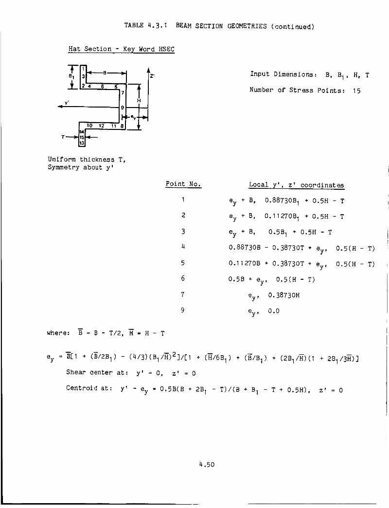
TABLE4.3.1 BEAMSECTIONGEOMETRIES(continued)

Hat Section - Key Word HSEC

i ill

1_ ej114 1,0 12

Uniform thickness T,

Symmetry about y'

where: B = B - T/2, H = H - T

Point No.

I

2

3

4

5

6

7

9

ey + B,

ey + B,

ey + B,

Input Dimensions: B, B I, H, T

Number of Stress Points: 15

Local 7', z' coordinates

0.88730B I + 0.SH - T

0.11270B I + 0.5H - T

0.SB I + 0.SH - T

0.88730B - 0.38730T + ey,

0.11270B + 0.38730T + ey,

0.5B + ey, 0.5(H - T)

ey, 0.38730H

ey, 0.0

0.5(H - T)

0.5(H - T)

ey = B--It+ (BI2B I) - (4/3)(B1/H)2]/[1 + (HI6B I) + (BIB I) + (2B1/H)(1 + 2B113H)]

Shear center at: y' = O, z' = 0

Centroid at: y' - ey = 0.5B(B + 2B I - T)/(B + B I - T + 0.5H), z' = 0

4.50

TABLE4.3.1 BEAMSECTIONGEOMETRIES(continued)

I Section - Key Word ISEC

8

B2

14

, Z'T

AI_--_!

71TTI9 _ A2

Input Dimensions: A I, A2, A3,

T I, T 2, T3

Number of Stress Points: 9

symmetry about z'

Point No.

I

3

4

6

7

8

9

Local y', z' coordinates

0. 38730A I , BI

0.0 ' BI

0" 38730A3, -B2

0.0 ' _2

0.0 , 0.8873_ I + 0.11 271B--2

0.0 , -0.11271B I - 0.8873B 2

-0.0

where BI = BI - 0.5TI,

Origin at shear center

Centroid at: y' -- 0

"B2 = B2 - 0"5T3

- 0"5(TI + T3) = BI + B2

z' = -B2 + [TIA1_2 ÷ 0.5T2(A2-TI-T3)(A2-TI)]/[TIAI+T2(A2-TI-T3)÷T3A3 ]

4.51

TABLE4.3.1 BEAMSECTIONGEOMETRIES(continued)

L Section - Key Word LSEC

Input Dimensions: A I,A2,T I,T 2

Number of stress points: 6

Z e

T 2

2

3

y'

5

6

Point No. Local _' ', z coordinate

0.88730A 1 , 0.0

0.11271A I, 0.0

0.50000_ I, 0.0

0.0 , 0.88730A 2

0.0 , 0.11271A 2

0.0 , 0.50000_ 2

where _I = AI - 0"5T2, _2 = A2 - 0"5TI

Origin at shear center: intersection of flanges

Centroid at :AI TIAI A2

y' = -- • , z' = m .

2 TI AI + T2A2 2

T2A 2

TIAI + T2A2

4.52

TABLE4.3.1 BEAMSECTIONGEOMETRIES(continued)

Thin Line Segment Beam - LSEG

END (Y_.yo<Z_)_ Z'

2

START lYe, Z

Input Dimensions = Y{, Z{, Y_, Z_, T.

Number of Stress Points = from 2 to 8.

Location of Stress Points: At Gauss points,

numbered in alternating sequence as shown.

Locations of points along length depends on number

of points used. See a handbook of math function

for exact locations.

Origin, shear center, and centroid: at mld-length,

Y' = (Y{ + Y_)/2

z, = (z{ + z )/2

4.53

TABLE4.3.1 BEAMSECTIONGEOMETRIES(continued)

Solid Circle - Key Word SCIR

Z _

y,I/f 1810'_ 11

-_ 2R

Input Dimension: R

Number of Stress Points: 24

"Point No. Local r, e coordinates

I

2

910

17

18

0.88730R, 70.98 o

0.88710R, 19.02 o

0.11271R, 19.020

0.11271R, 19.020

0.5R, 70.98 0

0.SR, 19.02 o

Points in second through fourth quadrants

are located by adding 90 0 , 180 0 ,

270 0 to the angles listed above.

symmetric about y', z'

Origin at shear center

Centroid at origin: y' = 0, z' = 0

4.54

TABLE4.3.1 BEAMSECTIONGEOMETRIES(continued)

Z' Solid Rectangle - Key Word SREC

9 13

11 15

4 12 16

2 10 14

A

7

B

6

I

Input Dimensions: A, B

Number of Stress Points: 16

Point No.

I

3

9

11

Local _' , z coordinates

0.430568A, 0.430568B

0.430568A, 0.169991B

0.169991A, 0.430568B

0.169991A, 0.169991B

sy_etric about y', z'

Origin at shear center

Centroid at orgiin: y' = O, z' = 0

4.55

TABLE4.3. I BEAMSECTIONGEOMETRIES(continued)

T Section - Key Word TSEC

Input Dimensions: A I,A2,TIT 2

Number of Stress Points: 6

Z +

A

8

TI

^,

i

TA2

Point No. Local y', z', coordinate

I O. 38730A I , 0.0

2 -0.38730AI, 0.0

3 0.0 , 0.0

4 0.0 ,

5 0.0 ,

6 0.0 ,

0.88730_ 2

0.11 271 A2

O.50000_ 2

where _2 = A2 - TI

Origin at Shear center: intersection of flanges

Centroid at: y' = 0 , z' =

0.5A2T2A 2

A ITI + A2T2

4.56

TABLE4.3.1 BEAMSECTIONGEOMETRIES(continued)

Two Dimensional Beam - Key Word TWD

_y" k

e

i, I

2

3

" N+I '

W

tT

Input Dimensions: W, T, N

Number of Stress Points: from 3 to 59 (odd)

Point locations: evenly spaced from

upper surface to lower surface, at

boundaries of an even number N of

equal thickness layers, from 2 to 58.

symmetric about y', z'

Origin at shear center

Centroid at origin: y' = 0, z' = 0

4.57

TABLE4.3.1 BEAMSECTIONGEOMETRIES(continued)

Z Section reversed - Key Word ZSCR

Ze

A 2

_l._A 1_,. _

Input Dimensions: A I,A2,T I,T 2

Number of Stress Points: 9

Equal flanges only

(anti-symmetric about y', z')

Point No. Local y', z' coordinates)

I 0.88730A I , -0.5_ 2

2 0.11 271A I , -0.5_ 2

3 0.50000A I , -0-5_ 2

7 0.0 , -0.38730_ 2

9 0.0 , 0.0

Q

where A2 -- A2 - T I

Origin at shear center

Centroid at origin: y' = 0, z' --0

4.58

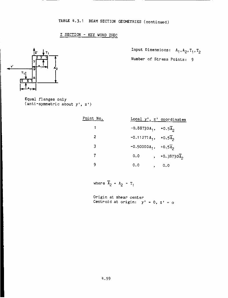
TABLE4.3.1 BEAMSECTIONGEOMETRIES(continued)

Z SECTION - KEY WORD ZSEC

yt

Equal flanges only

(anti-symmetric about y', z')

Input Dimensions: A I,A2,T I,T 2

Number of Stress Points: 9

Point No.

I

2

3

7

9

Local y', z' coordinates

-0.88730A I, +0.5_ 2

-0.I 1271A I , +0.5_ 2

-0.50000A I , +0.5_ 2

0.0 , +0. 38730_ 2

0.0 , 0.0

where _2 = A2 - TI

Origin at shear center

Centroid at origin: y' -- 0, z' = o

4.59

4.3.3.6 BeamLoads (Group I)

The following mechanical loads may be applied to the beamelement:

CONC - Concentrated forces and momentsapplied at specific nodes in theglobal directions.

BMLO - Distributed line load in the beamlocal transverse directions.A linear variation of the distributed load between nodes is assumed.

These loads are discussed in Section 4.6.

4.60

4.3.3.7 BeamOutput

This paragraph shows examples of typical output generated; these are distinct tothe beamelement.

Beam Connectivit_

HEMBERBEAM ELEMENTS

NODE X NODE J NODE K

i 10B 102 10810_ 102 1B8

106 104 108108 106 102

Z 200 202 208204 202 208

i 206 20* 206208 206 20210 300 304 31612 306 304 31614 312 308 31616 316 312 304IS 40O 408 40621 410 408 40622 422 410 40626 416 422 406• _ 414 406 422_f 406 400 42241 6000 108 31162 208 6000 31143 6002 208 31144 316 6002 3114S 600_ 316 31146 414 6004 31147 8000 316 311&8 8002 8000 31149 8004 8002 311SO 406 8004 311S1 101 108 10852 103 101 10853 105 103 10854 10S 108 10155 201 200 20856 203 201 20857 205 203 208$8 20_ 208 20160 303 300 31663 307 303 31664 311 307 316

3066 311 316 40_68 ,_3 .0071 409 403 *0672 411 409 40673 411 414 406

NOTE: The third node shown is the pointer node that defines the local y direction in

the beam cross section.

4.61

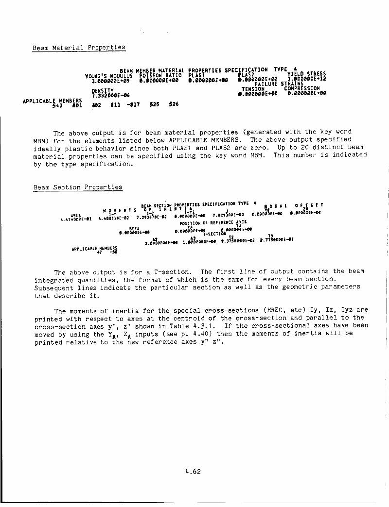
Beam Material Properties

BEAN NENBER NATERIAL PROPERTIES SPECIFICATION TYPE 6YOUgGtS NODULUS POISSON RATIO PLAS1 PLAS2 YIELD STRESS

3.O_D_gE÷09 O.OO0_g_E÷OB O.OBODOBE+H O.O_O_E+BO 1.B_OO_gE÷12FAILURE STRAINS

DENSITY TENSION CONPRESSION7.3320DOE-06 I.t_D_gE+IO O.O_OO_gE÷Bg

APPLICABLE NEHBERS543 B01 a02 gll -817 $25 $26

The above output is for beam material properties (generated with the key word

MBM) for the elements listed below APPLICABLE MEMBERS. The above output specified

ideally plastic behavior since both PLASI and PLAS2 are zero. Up to 20 distinct beam

material properties can be specified using the key word MBM. This number is indicated

by the type specification.

Beam Section Properties

|EAN SECTION PROPERTIES SPEC|FICJ_TION TYPE 6 f S E T

AREA ]-Y T.2936_IE-'ID2 _ D E*'-I_ T.e29JDeE--I_$,.6?,ooeE-'ll 4.6BBEleE--112

FOS]TZON OF REFERENCE AXISBETA YA ZA

I.eB_e_BE_IIO O.eeeODeE_.sEC-t]_i I_e_N_E+I_

A3 AS T2 T$2.egDgOOOE'H)B 1.1H_D_BDBE'q_ 9.375ee._l_E-02 _.775001_E"el

APPLIC_LBLE NEMBERS67 -5l

The above output is for a T-section. The first !ine of output contains the beam

integrated quantities, the format of which is the same for every beam section.

Subsequent lines indicate the particular section as well as the geometric parameters

that describe it.

The moments of inertia for the special cross-sections (HREC, etc) Iy, Iz, Iyz are

printed with respect to axes at the centroid of the cross-section and parallel to the

cross-section axes y', z' shown in Table 4.3.1. If the cross-sectional axes have been

moved by using the YA' ZA inputs (see p. 4.40) then the moments of inertia will be

printed relative to the new reference axes y" z".

4.62

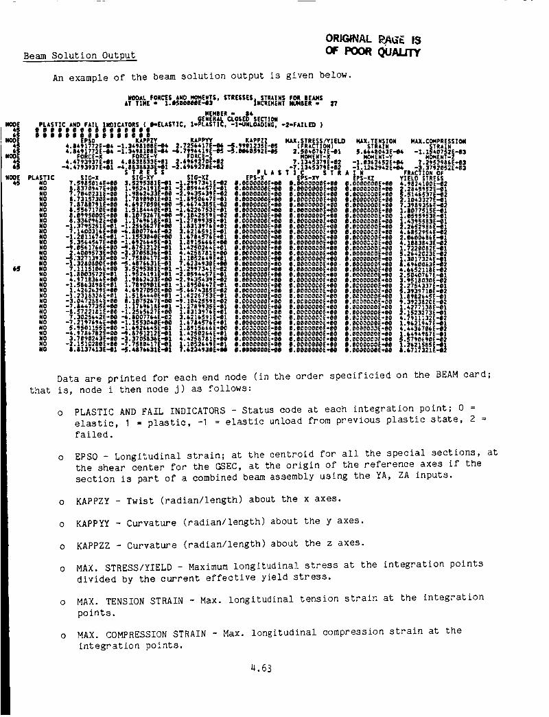
Beam Solution Output

ORIG A[. ISOF PORe QUAJ.JTy

An example of the beam solution output is given below.

NOOE PLASTIC4S NO

NONONONONOMONONONONONONONONONO

6S NONONONOMRNONONONONONONONONONONO

NOOAL FORCES AMD MOMENTS, STRESSES, STRAINS FOR |EAHSAT T|M[ " 1._00_1E-43 INCR(MENT NUI4BER ,, 2?

MEMBER m |4GENERAL CLOSED SECTION

PLASTIC AND FAIL IMD|CATORS ( O*[LASTIC, 2-PLAST|C, -|*'UNLOAOIMGt -2..FAILED )ill I liQ ellllfillliilililillllili

EPS0 KAPPZY KAPPYY KAPPZZ HAX. STRESS/YI ELD KkX. TENS ZON4.8491772E--II_. -1.3&981eRE-D4 2.72S6417E--I_ -5.990123SE...1_ (FRACTION) STRAIN4.8491772E-04 -I.34981BOE44 -6.7996419[-_5 -_.N6OSt2E-45 2.5G40767£-41 5.66_8043E-04

FORCE-X FORCE-Y FORCE-Z IqOIAENT-X 140_AENT-Y4.4793937E._.111 4.8S38833E.qW| 2.6969270E÷R2 7.134S379E+1_2 -1.1D362652E,'R4

-A.4793937E+01 -4.8838J33E._..01 -2.696927BE_'-Ih_ -7.1345379E+92 -1.).262942E.¢,.1_S T R e S S P L k S T X C S T R A ! N FRACTION OF

SIG*X SIG-XY SIG-XZ EPS-X EPS-XY [:PS-XZ YIELD STRESS7.5985016,E÷'llg 3._;295381E-el -1.299736,1E."e2 il.Ol_OOOoO£.q.eO II.BOOODDOE+BB ID.DO;_OC_OE-"OB A.De2411)OE-028.8370947E*OO 1.9524191E._-01 -2.059*&STE-ISl ID.O00OOOO[_..Oi_ e.eeooeeee,,eo e.eoeo_OE,-ee 2.2865952E-el7.7eAo231E*ee 1.9862433E+OiJ -2.943S&39E-m2 e.eoeoi_oo£,ee e.eeeoeooE,,i_ 11.6ooc_DOE+60 S.5146537E-'e28.T31573oE','eo 1.?8DO)DOle+g1 -1.11950647E-91 e.eeoooooE_.ise e.e_ocooot+,e e.eeeooooe-ee :_.1043327E-B17.8788791E+00 4.6927i55eE._tH_ -aJ.667435SE-Q;_ iD.BOOOOOOE,.00 e.£i_OOl_DOE*Ol_ e.BeoooooE÷ee 7.3989356E-.e28._;56717i_E.qH_ 1.51S44*eE,-I)1 -1.6226753E-D1 O.i_OOO(_OOE,.el) e.eeooeeeE..t_i_ I.eoeceDeE*ee 1.807751SE..-II18.e995eoee.ee 8.1075267E._-I_ -9.10425SqE-'_2 e.eooeOOOE..l_ e.eoo_eooE,.ee O.OOOOODDE*OO 1.059_DS3E-,gl8.33£0962£*'eil 1.1769618E'q_1 -1.2769935E-01 O.OOOO_OOE._i_O il.eOOOO_E,-O0 i_.i_DOOCOOE',_8 1.4395583E-.01

-1.3795251E.,gl -1.256_&27E+Oil |.$313976£+01 o.eooooooE..ee R.I)OCODOOE,*O_ o.e_o_eOOE._e 2.2652986E-t_17.1400316£+0B -_.8_7764E-B2 3.&216591E-01 O._,OODOOOt:*.08 O.BI_OOO_OE,*90 B._ODCC,COE+I_O 4.&SS29SkE-t_2

-).2_11674E._01 *l.l_53D40E,_O 1.6?84576E÷el R._DOOOOE*D8 i).l_ODOeOOE,_.DB i_.ODDOODOE._,._B 2.66_OSSSE-Ill_.3_64547E,*,0i_ -1.69266_,SE-01 1.11915666E*,4_1 O.eODODOOE*_i_ I).OODODe,OE,*,90 O._OO0_,_E*tH_ 4.1H3843E-02

-9.B561766E.,-I_O ,-'9.11751212E.-gl 1.,_250264E._1 II.l_OOOOOg,S*9i_ e.l_DeOOOOS*Ol) I_.eOOCOOOE.,_e 1.7229082E.-,_12.4009573E.q_ -3.37BS836E-01 4.4256781E.t_1_ O.DOl_OOe_[_l_ iS.l_O_._OOE...Dt_ e.l_Oi)OOOOE_-iH) 5.2642C23E-i_2

_j.3271393E._'Oe -7.758e41?E-01 ;.leS26*tE*l)l I.eOOOOOOE.,eO R.eo_ooeoE-.-ee I).OOOOOOOE-'eg 1.31_17324E-'el-1.32808_OE.q_ -JJ.A876631E--B1 7.623493DE+OR) O.i)ODOOOOS*ilO e._eoo_ooE.ee II.i)oDoooo_._oi_ |.6961_063E-._27.1115106E*e8 3.5295581E-01 -1.2997341E-_2 It.I_OOCO00£'_-BO 0.OOOOOODE,,eO 11.OOO_OOO£*l_O k.6652118E-62-1.SBO3S72E','O1 1.952_',191E÷111 -2.1_J944S?E-01 Q.DO_OOOOE÷BO I).OOOO000E÷OB g.l_0O00OOE._i_ 2.SOkl_?67E--_l

4.9718364E,'1_ I.D662633E÷BO -2.9435439E-02 I_.eeOoooOE.ee e.eoooeooE÷eo II.eOOODOOE*eO 3.951BO3OE-e2-1.5663J_DSE"el 1.78fOIBle-g1 -1.8950647E-el II.l_OOOOOOE.'Og O.IPOOOOCOE'_Be I_.ODOOCOOE*.BI) 2.2754337E-01

1.4262639E'_00 4.6927050E."_0 -aJ.667_,385E-'_2 B.BOOOCe_OE*I_O E.BI_ODOO_E',-OD I_.I_DDDOOD£','BO 5.393971B[-02-1.2318326E.'1_1 1.518_,4_*OE'*el -1.6226TS3E-R1 e.OOOOOOOE.-eO e.oco_oo2E.,.e,o II.O_OOOCE.,.OO 1.8982645E-el-3.0472554E",Ol_ 8.1_?_267E*1)_ -9.11_42_59E-1_2 II.DCDDC,i)0E*B0 I).I_i_CO0CE"00 O._CDODCO[*0;_ 9.392352CE-e2-7.R&.k773SE.*t)O 1.17&961BS.q_l -1.2"/89935E-B1 O.iPDOOOOOE.,._ e.eeooOOOE*ee e.eo_coooE*eo _,.427";138E-.el-8.5"/2_lelE,.ee -I.2S_S_27E÷ee 1.8313976E.,-01 o.eeoDOOOE-ee II.l_OCooooE,.ee e.eooooooE*ee 2.1S23273E-el

7.302S642E.*eB ,-_.BOO77&AE-102 3.k216591E-.el e.oeoeooo[,,.ee e.ee_ooocE÷ee e.e_ec_oe-eo 4.7911132[.-_2-7.2197_DkE÷OO -I.1553048E'*'BO 1.67114S76£*111 O.eODOOC,OE._B O.O_ooOOOE÷l_9 B.OCO_ODOE-O0 1.96219_TE-BI

5.9501155E.,._0 -1.k92k645E-'_l 1.891566_-E*.eO I_._O_OOO£*O_ g._c(_OC_,E.'eO O._D_OO_DE*O0 4.A&367e_E-_2-6.9786782E_'DD -9.$7S1212E-01 1.k2S_264E*el O.I_OOOOOOE._O0 $.I_DD_OE*BO O.eOOOOODE-t)B l.&At_,DS7E-el

3.?_90243E_"_0 -3.370S836E-I)1 4.*258781E"OO e.l_O_ooooE.-ee O.B_DDODOE,,.BB O.oco_D_DE,,.Bo 5.S790690E-_2-2.151C28_E*O8 -7.758Bkl?E-01 ],.lOS2_49E,,,.el 1_.oeoc_)_oE,,.ee B.OODOee,OE.,.BB il.i_OOOODDE,,,t_l_ 1.2621SSSE-gl

ll.8137413E-41 -S.4876631E.-II1 7.623493eE_iHI II.Bi)OeDOOE,DO e.l_Ot_O_O£_l_O II.eO;)i_DOO£-i)8 _1.6717321E-_2

I,U,X.COMPRESSXONSTRA|N

-1.1_407_2E-.R3HOHENT-Z

7.295_98_E-'.03-3.3792052[--63

Data are printed for each end node (in the order specificied on the BEAM card;

that is, node i then node j) as follows:

o PLASTIC AND FAIL INDICATORS - Status code at each integration point; 0 =

elastic, I = plastic, -I = elastic unload from previous plastic state, 2 =

failed.

O EPSO - Longitudinal strain; at the centroid for all the special sections, at

the shear center for the GSEC, at the origin of the reference axes if the

section is part of a combined beam assembly using the YA, ZA inputs.

o KAPPZY - Twist (radian/length) about the x axes.

o KAPPYY - Curvature (radian/length) about the y axes.

o KAPPZZ - Curvature (radian/length) about the z axes.

o MAX. STRESS/YIELD - Maximum longitudina_ stress at the integration points

divided by the current effective yield stress.

o MAX. TENSION STRAIN - Max. longitudinal tension strain at the integration

points.

o MAX. COMPRESSION STRAIN - Max. longitudinal compression strain at the

integration points.

4.63

Beam Solution output (continued from previous page)

o FORCE X, FORCE Y, FORCE Z - Longitudinal (x) and transverse forces.

o MOMENT X, MOMENT Y, MOMENT Z - Torsion (about x) and bending moments (about

the y and z axes).

The following additional data are printed only if the MSTR card is specified in

the Group A input:

o SIG X, SIG XY, SIG XZ - Longitudinal and shear stresses at each integration

point.

o EPS X, EPS XY, EPS XZ - The plastic part of the Longitudinal and shear strains

at each integration point.

Those quantities that depend on the location or orientation of the y and z axes

(EPSO, KAPPYY, KAPPZZ, FORCE Y, FORCE Z, MOMENT Y, MOMENT Z, SIGXY, SIGXZ, EPSXY,

EPSXZ) are calculated with respect to the centroidal axes.

If the MSTR card is omitted from the Group A input, the short form beam output

will be used for all beams, which deletes the stress and strain data at each

integration point. However, the maximum stress/yield stress ratio and the maximum

strains are given, which should be sufficient in most cases. This default condition

will cause the printing of four beam element solutions per page, compared to only one

per page if the MSTR card is used, and will greatly reduce the print-out in cases with

many beam elements.

In the event that a beam element fails (when all its integration points at either

node fail), its solution output is deleted from the print-out.

4.64

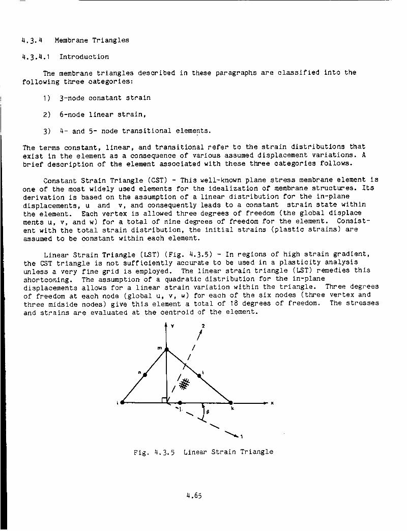
4.3.4 MembraneTriangles

4.3.4.1 Introduction

The membranetriangles described in these paragraphs are classified into thefollowing three categories:

I) 3-node constant strain

2) 6-node linear strain,

3) 4- and 5- node transitional elements.

The terms constant, linear, and transitional refer to the strain distributions that

exist in the element as a consequence of various assumed displacement variations. A

brief description of the element associated with these three categories follows.

Constant Strain Triangle (CST) - This well-known plane stress membrane element is

one of the most widely used elements for the idealization of membrane structures. Its

derivation is based on the assumption of a linear distribution for the in-plane

displacements, u and v, and consequently leads to a constant strain state within

the element. Each vertex is allowed three degrees of freedom (the global displace

merits u, v, and w) for a total of nine degrees of freedom for the element. Consist-

ent with the total strain distribution, the initial strains (plastic strains) are

assumed to be constant within each element.

Linear Strain Triangle (LST) (Fig. 4.3.5) - In regions of high strain gradient,

the CST triangle is not sufficiently accurate to be used in a plasticity analysis

unless a very fine grid is employed. The linear strain triangle (LST) remedies this

shortcoming. The assumptio_ of a quadratic distribution for the in-plane

displacements allows for a linear strain variation within the triangle. Three degrees

of freedom at each node (global u, v, w) for each of the six nodes (three vertex and

three midside nodes) give this element a total of 18 degrees of freedom. The stresses

and strains are evaluated at the centroid of the element.

m

i v

Y 2

!

v ! X

Fig. 4.3.5 Linear Strain Triangle

4.65

Transitional or Hybrid Triangles (HST) - In transition regions, i.e., regions inwhich stresses and strains change from rapidly varying to slowly varying, it becomesconvenient and efficient to switch from linear strain triangles to constant straintriangles. This is accomplished by using four- and five-node triangles to maintaincompatibility with both the CSTand LST elements. For these mixed formulation hybridelements, the displacements along edges may vary quadratically or linearly, dependingon whether an LSTor CSTtriangle is contiguous to the respective sides.

4.66

4.3.4.2 MembraneInput Data

The input data for the membranefamily of triangular elements are specified withthe following input cards:

Group Keyword Required

C TRIM Yes

Comment s

Element identification and

connectivity.

H MATI one

MAT2 required

MAT3

One of these card types is used

to specify material properties.

H THIK Yes Element thickness.

H MBET No Angle in de_rees between

local x-axis and principal

l-axis for material orthotropy.

I CONC No Concentrated loads at nodes.

4.67

4.3.4.3 MembraneConnectivity (TRIM, Group C)

The nodes for the triangular family of elements are specified around the peri-meter beginning with a major (vertex) node followed by a minor (midside) node and thenmajor and minor nodes as shown in Fig. 4.3.5. The absence of a minor node must beindicated by a zero or blank field in the proper position. Minor nodes must be midwaybetween the major nodes. However,lt is not necessary to manually calcula--_-thecoordinates for a mldslde node, since the program does this calculation automaticallyand disregards any such coordinates input by the user. In fact, the mid-side nodescan be omitted completely from the Group D (coordinates) input. The local x-axls isdefined as the direction of the vector from node i to node k as specified in theGroup C input. The local y-axis is the in-plane normal to the x-axis towards nodem. The memberidentification can be any number of up to five digits. These numbersneed not be consecutive but must be unique for the model.

Example: Five NodeTriangle0........ I ......... 2......... 3......... 4......... 5 ......... 6......... 7......... 812345678901234567890123456789012345678901234567890123456789012345678901234567890TRIM 27 5 7 I 0 11 12

11

12_10

5

4.68

4.3.4.4 MembraneMaterial Properties (Group H)

All material properties are constant within the element.available:

MATI

MAT2

MAT3

Three input options are

- Material isotropy for elastic and plastic behavior with ideallyplastic behavior or linear or nonlinear kinematic hardening.

- Orthotropic, Elastic-ideally plastic behavior.

- Orthotropic, Elastic-linear or nonlinear hardening plasticity.

Oneof these specifications must be included for each TRIM element. Up to 20different sets of plane stress material input cards may be used, totalled over MATI,MAT2,and MAT3types. Three types of plastic behavior can be considered, as follows:

Input Parameters

PLASI PLAS2 Types of Plasticity

0.0 0.0 Perfect plasticity (zero modulus in plastic range)

Et/E 0.0 Linear strain hardening parameter = Et/E, with E t equal

to the slope of the uniaxial stress versus strain curve

in the plastic range

n _0.7 Nonlinear strain hardening with Ramberg-Osgood form of

the uniaxial stress-strain curve, see p. 4.19.

These plane stress material property parameters should ideally be taken from

curves of engineering stress versus true strain. Engineering stress should be used

because the program does not change the thickness due to Poisson's ratio under in-

plane strains. Using engineering strain will involve errors whose magnitude is

approximately half the strain (e.g., 10% strain gives a 5% error), and in many cases,

this error is acceptable. The material stiffness integrations will be affected only

for the nonlinear hardening materials, because the tangent moduli in the plastic range

are constant for the linear hardening and perfectly plastic materials. Stresses will

not be significantly affected by this strain error in the case of perfect

plasticity. Therefore, using engineering stress-strain curves should be adequate for

most purposes. Tension and compression properties are assumed to be the same, except

for failure.

4.69

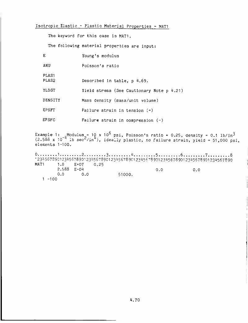
Isotropic Elastic - Plastic Material Properties - MATI

The keyword for this case is MATI.

The following material properties are input:

E Young's modulus

ANU Poisson's ratio

PLASI

PLAS2 Described in table, p 4.69.

YLDST Yield stress (See Cautionary Note p 4.21)

DENSITY Mass density (mass/unit volume)

EPSFT Failure strain in tension (+)

EPSFC Failure strain in compression (-)

106Example lb/in 3I:4Modulus = 10 x psi, Poisson's ratio = 0.25, density = 0.1

(2.588 x 10- lb sec2/in4), ideally plastic, no failure strain, yield = 51,000 psi,elements 1-100.

0 ........ 1......... 2 ......... 3 ......... 4 ......... 5 ......... 6 ......... 7 ......... 8

123456789_123456789_123456789_123456789_12345_789_123456789_123_56789_123456789_

MATI 1.0 E+07 0.25

2.588 E-04 0.0 0.0

0.0 0.0 51000.

I -100

4.70

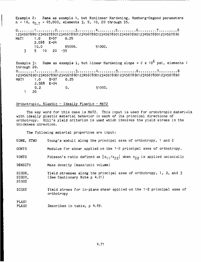
Example 2: Sameas example I, but Nonlinear Hardening, Ramberg-Osgoodparametersn = 10, _0.7 = 65,000, elements 3, 5, 10, 20 through 35.

0 ........ I ......... 2 ......... 3......... 4......... 5 ......... 6 ......... 7 ......... 8

123456789_123456789_123456789_123456789_123456789_123456789_123456789_123456789_

MATI 1.0 E+07 0.25

2.588 E-04

10.0 65000. 51000.

3 5 10 20 -35

Example 3: Same as example l, but Linear Hardening slope = 2 x 106 psi, elements I

through 20.

0 ........ I......... 2 ......... 3......... 4......... 5 ......... 6 ......... 7 ......... 8

12345678 901 2345678 9012345678 901 2345678 9012345678 9012345678 9012345678901234567890

MATI 1.0 E+07 0.25

2.588 E-04

0.2 O. 51000.

I 20

Orthotropic, Elastic - Ideally Plastic -MAT2

The key word for this case is MAT2. This input is used for orthotropic materials

with ideally plastic material behavior in each of its principal directions of

orthotropy. Hill's yield criterion is used which involves the yield stress in the

thickness direction.

The following material properties are input:

EONE, ETWO

GONTO

VONTO

DENSITY

Young's moduli along the principal axes of orthotropy, I and 2

Modulus for shear applied on the I-2 principal axes of orthotropy.

Poisson's ratio defined as I_11/_221 when e22 is applied uniaxially

Mass density (mass/unit volume)

SIGOX,

SIGOY,

SIGOZ

Yield stresses along the principal axes of orthotropy, I, 2, and 3

(See Cautionary Note p 4.21)

SIGXY Yield stress for in-plane shear applied on the I-2 principal axes of

orthotropy

PLASI

PLAS2 Described in table, p 4.69.

4.71

EPSFTI

EPSFT2

EPSFCI

EPSFC2

Failure strain in tension in the I direction (+)

Failure strain in tension in the 2 direction (+)

Failure strain in compression in the I direction (-)

Failure strain in compression in the 2 direction (-)

Example: Ortho_ropic material, Density = .I lb/in 3 (2._88 x 10-4 lb sec2/in4),EI = 10.55 x 10 v psi, E2 = 7.61 x 10 _ psi, G12 = 4 x 10 v psi, n12 = .33, in-plane

normal yield stresses in 1,2 directions = 61,000, 52,000 psi, in-plane shear yield =

31585 psi, yield in thickness direction = 61,000 psi, ideally plastic behavior, no

failure, elements 26 through 28 and 74 through 76.

0 ........ I ......... 2 ......... 3 ......... 4 ......... 5 ......... 6 ......... 7 ......... 8

1 2345678901 2345678901 2345678901 2345678901 2345678901 2345678901 2345678901 234567890

MAT2 10.55 E÷06 7.616

2. 588 E-04

0.0 0.0

61 000. 52000.

0.0 0.0

26 -28 74 -76

E+06 4.0 E+06 0.33

0.0 0.0

61 000. 31 585.

Orthotropic, Elastic - Strain Hardening Plastic - MAT3

The MAT3 input is used for orthotropic materials with linear and nonlinear

hardening behavior. The approach taken to implement this feature is based on the use

of Hill's yield criterion and a hardening behavior in the two principal normal

directions and in the principal shear direction. Either a Ramberg-Osgood

representation for nonlinear hardening behavior or a linear hardening behavior can be

used in each principal direction of orthotropy. The first three cards of input for

this feature are the same as for MAT2. The fourth and fifth cards contain input for

the hardening parameters. None of the components can be specified as ideally plastic

although linear and nonlinear plastic behavior can be mixed.

4.72

The following material properties are input:

EONE,ETWO

GONTO

VONTO

DENSITY

SIGOX,SIGOY,SIGOZ

SIGXY

PLASIXPLAS2X

PLASIYPLAS2Y

PLASIXYPLAS2XY

EPSFTIEPSFCl

EPSFT2EPSFC2

Young's moduli along the principal axes of orthotropy

Modulus for shear applied on the I-2 principal axes of orthotropy

Poisson's ratio defined as I¢11/_221 when _22 is applied uniaxially

Mass density (mass/unit volume)

Yield stresses along the principal axes of orthotropy; 1,2,and 3see cautionary note p 4.21)

Yield stress for in-plane shear applied on the I-2 principal axes oforthotropy (see cautionary note p 4.21)

PLASI for I axis of orthotropy (see table p 4.69)PLAS2for I axis of orthotropy (see table p 4.69)

PLASI for 2 axis of orthotropy (see table p 4.69)PLAS2for 2 axis of orthotropy (see table p 4.69)

PLASI for shear on I-2 axes of orthotropy (see table p 4.69)PLAS2for shear on I-2 axes of orthotropy (see table p 4.69)

Failure strain in tension on the I axisFailure strain in compression on the I axis

Failure strain in tension on the 2 axisFailure strain in compression on the 2 axis.

4.73

Example: Orthotropic material, Linear hardening in the principal I direction, non-linear hardening in the 2 and I-2 shear directions, elements 1-100.

General: Density = .I ib/in 3 (2.588 x 10-4 lb sec2/in4), Poisson's ratio 12 = 0.3

Normal l-direction: Modulus _ 10.7 x 206 psi, yield _ 53,500 psi, linear hardeningslope _ .394 x 10v psi, no failure

Normal 2-direction: Modulus _ 21.4 x 106 psi, yield = 32,000 psi, nonlinearhardening n _ 10, _0.7 _ 46,600 psi, no failure

Normal 3-direction: Yield _ 53,500 psi

Shear 1-2-direction: Modulus _ 3.923 x 106 psi, yield _ 22,000 psi, nonlinearhardening n _ 9.675, _O.7 _ 28,800 psi, no failure

O........ I ......... 2 ......... 3......... 4......... 5 ......... 6 ......... 7 ......... 81234567890123456789012345678901234567890"1234567890123456789012345678901234567890MAT3 I .07 E+07 2.14 E+07 3. 923 E+06

2.588 E-04 0.00.0 0.05.35 E+04 3.20 E+043.68 E-O2 O.02.88 E+04I- 100

0.30.0

5.35 E+04 2.2 E+04

10.0 4.66 E+04 9.675

4.7a

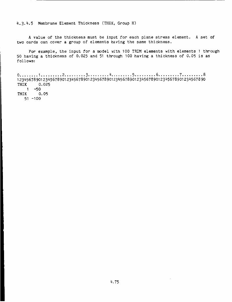
4.3.4.5 MembraneElement Thickness (THIK, Group H)

A value of the thickness must be input for each plane stress element. A set oftwo cards can cover a group of elements having the same thickness.

For example, the input for a model with 100 TRIM elements with elements I through50 having a thickness of 0.025 and 51 through 100 having a thickness of 0.05 is asfollows:

0........ I ......... 2......... 3......... 4......... 5......... 6......... 7 ......... 8123456789_123456789_123456789_123456789_123456789_123456789_123456789_123456789_THIK 0.025

I -50THIK 0.05

51 -100

4.75

4.3.4.6 Orientation of Axes of Material Anlsotropy (MBET,Group H)

The element stiffness matrices are calculated with respect to an element localaxis system referred to as x, y in Fig. 4.3.5. For this purpose orthotropic materialproperties must be transformed from the material's principal orthotropic axis system,shown as 1,2 in Fig. 4.3.5, to the element local coordinate axis system through theangle B, the angle between the x and I axes, according to the transformation;

_x Q{I QI2 Q_6 Ex

where

_y -- QI'2 Q22 Q26 Cy

_xy Q_6 Q26 Q_6 exy

(4.3.13)

Q_I _ Q11c°s4B + 2(Q12 + 2Q66) sin2B c°s2 B + Q22sin4 B

Q22-- Q11sin4B + 2(Q12 + 2Q66) sin2B c°s2 B + Q22 sin4 B

Q_2 " (Q11 + Q22- 4Q66) sin2B c°s2B + Q12(sin4B +c°s48)

Q_6 _ (Q11 + Q22- 2Q12- 2Q66) sin2B c°s2B + Q66(sin4B + cos4B)

Q_6 _ (Q11 - Q12- 2Q66) sinBc°s3B + (Q12 - Q22 + 2Q66) sin3B cosB

Q26 _ (Q11 - Q12- 2Q66) sin3Bc°sB + (Q12 - Q22 + 2Q66) sins cos3B

(4.3.14)

and

°I Q11 Q12 0 cI

_2 -- QI2 Q22 0 E2

e12 0 0 Q66 e12

(4.3.15)

All the stress and strain calculations are calculated in the material system andthen transformed into the element local system for the output. It should be notedthat the angle 8 is constant for each element and is not updated due to geometrychanges during the course of the analysis.

If the body is isotropic or if the local and material axes coincide, then B istaken as zero by default and this input is not necessary. Note that 8 is from the l-axis to the x-axis, with the sign convention determined by a right-hand rotation aboutthe z-axis.

4.76

As an example, if the angle between the local x and the material 1 axes is 45degrees for elements I, 3, 5 ... 21 then the input is:

0........ I ......... 2......... 3......... 4......... 5......... 6......... 7......... 8123456789_123456789_123456789_123456789_123456789_123456789_123456789_123456789_MBET 45.0

I -2 -21

4.77

4.3.4.7 Membrane Loads (Group I)

The following mechanical loads may be applied to the membrane elements:

CONC - Concentrated forces and moments applied at specified nodes in the global

directions in the units of force or force times length.

These are discussed in Section 4.6.

4.3.4.8 Membrane Output

This section shows examples of typical output generated for the triangular

membrane element.

Membrane Connectivity

MEHBERTRIANGULAR MEMBRANE ELEMENTS

NODE I NODE J NODE K NODE L NODE M NODE N

5 11 75 1206 75 74 1287 74 73 1208 73 86 1209 76 23 92

10 76 92 14111 74 75 2212 92 22 7513 69 70 1714 27 17 7015 19 18 2716 27 70 1917 71 19 7018 72 20 7119 19 71 2e20 12 76 14121 75 11 1222 73 74 2223 21 73 2224 16 32 1525 14 15 3226 15 90 1627 91 16 9028 5 91 429 90 4 9130 15 14 8931 89 90 1532 3 4 9033 90 89 334 88 2 335 3 89 8836 32 88 8937 89 14 3238 91 S 639 6 87 9140 16 91 8741 87 72 1642 71 16 7243 16 71 7044 32 16 7045 70 69 3246 69 84 32

NOTE :The nodes connecting the element are printed in a counterclockwise order, i.e,

first a major (vertex) node followed by a minor (midside) node, if present

in the absence of a midside node the column for the midside node is blank

4.78

Membrane Element Material Properties

NAT1HATERIAL PROPERTIES SPECIFICATION TYPE 2YOUNGtS HOOULUS POISSON RATIO PLAS1 PLAS2

1.120000eE+87 3.3300880E-81 8.OBOeB88E+e8 8.88_088E+1_FAILURE STRAINTENSION COHPRESSION

YIELD STRESS DENSITY5.B1380888+84 2.5888880E-II4 8.88_08808"q18 0.081_008E÷88

APPLICABLE HEHBERS1001 -1026 21_1 -2026 3001 -3826

This output indicates ideally plastic behavior (since both PLASI and PLAS2 are

zero) for an isotropic material with no failure (infinite strain capability). This

printout is generated when specifying material properties with a MATI card.

Membrane Element Thickness

THICKNESS TYPE 1 IS 2.SOB81N_BE--82THE NUHBER OF LAYERS IS 2

APPLICABLE HEHBERS1_81 -lm26 2001 -2826 3001 -3026

The above example is for the specification of a thickness of .025. The number of

layers is ignored for membrane elements (TRIM), and defaults to 2 layers if not

specified on the THIK card.

4.79

OmGINRL AGE ISOF POOR QUALITY

Membrane Solution Output

The output as shown below gives the plasticity indicator, the stresses, total

strains, and plastic strains in the local axis system (Fig 4.3.5), the ratio of

maximum principal stress divided by the current effective yield stress, and the number

of subincrements used in satisfying the constitutive laws. All these data are

calculated for the single integration point at the centroid of the triangular

element. A plasticity indicator of NO indicates an elastic element, YES indicates a

plastic element, and UNL indicates an elastic unloading from a previously plastic

state. A failed element is deleted from this print-out.

MEMBER PLASTIC

5 NO& NOT NO8 NO9 NOIe NO11 NO12 NO13 NO14 NO15 NO16 NO17 NO18 NOI_ NO2_ NO21 NO22 NO23 NO24 NO25 NO26 NO27 NO2B NO29 NO30 NO31 NO32 NO33 NO34 NO35 NO36 NO3? NO38 NO39 NO40 NO41 NO42 NO43 NO• 4 NO45 NO4k NO67 NO68 NO49 NO_o NO

STRESSES AND STRAINS FOB TRIANGULAR MEMBRANESAT TIME., 4,1)000000E43 INCREMENT NUMBER .... 80

STRESS TOTAL STRAIN PLASTIC STRAINX Y XY X Y XY X Y XY

-1.23ee+|3 *B.SI_3E'HD2 -'&.lB&E"01 -3.25BE-e5 -_..6e4E-IP_ -aJ.3G1E-I_$ e.eeeE.*'BB e.eOOE-_ e.BeeE._IP-2.191E'03 *3.031E'*'03 _.3(_5E*03 -4.273E-i)5 -7.911E-05 1.131E-04 e.oooe*oe |.BO(_E*DO e.OOOE"OO

6.040£'*'02 -2.235E,"_3 B.015E','02 3.5_1E-05 -?.853E-eS 4.946E'-05 0.800E*00 O.O_OE'*O0 g.O_OE'.'O0-3.&kTE÷tD3 *2.886E*03 7.383£_'1P1 -9.271E-O5 -_.972E-05 0.399E-t_ II.i_BOE_'i_lD 0.OOO£'_l)O 0.000£'_00

2.126E-"02 *2.506E*03 -3.519E'*'02 3.214E-B5 -B.566E--05 -3.050E-05 O.OOOE.,OO O.OeOE.,.OO O.OOOE,*.OO-2.426[--_3 5.607E.*-02 I._45E'*'02 -B.067E-05 4.295£-05 1.252E-_S O.OOeE.*'eO O.0OOE-,.00 i.OOOE.*.O0-1.610E+03 --_.257E,"02 3.273E.,.03 -,L.273E'_5 -1.O0?E-B? 2.830E'-04 O.eOOE,'OO e.I)BOE'*'BO O.BOO[_'OB-3.139E÷03 -8.998E*02 2.244E÷i03 -9.5&&E-1_5 1.398E-I_ 1.858E-'04 O.i)BOE._..eB I).I)OOE,¢*-BO |.BI)BE*l_-6.896E*03 -1.825E*03 -2.058£+03 -1.849E-04 1.183£--e7 -1.7B3E-'04 O.OOOE*BD ll. OOOE*i_B B.BDOE_'iDO-3.303E*t_3 -9.926E*02 3.315E'*'02 -1.i)_2E-04 -'6.k3SE-'QB 2.874E"05 ID.O00E"*_O I_.l_OOE_'tH_ I_,.BOOE*e*O

1.348E'*'03 -._.932E+02 -'6.617£*iP3 5.006E-'05 -3.326E-05 --_.562E--04 O.OOOE'*iH_ $.i)OeE*l)O O.OeOE*l)o-2.7#2E'*'03 -9.19BE*_3 5,994E'02 -6.BqTE-eB -2.790E-04 5.195E-05 e,eeoE*eo e.000E',-OO i.OOOE.*.eO

,;.22_£-,03 -7.&25E*_3 7.773E-0_ 2.171E-04 -2.944[-_4 _.737E-15 _.Be_E'*'BB _.B00E'*'_e i.BOeEoBO2._79E÷02 -&.B3?E'*'_3 -1.122['*'02 7.k&BE-OS -2.3_4E-04 -9.722E-IH; B.BOeE*OB _.i_00E.*.#_ i.BOOE*004.2ALE','03 -7.5_,9E÷03 -1.489E+03 2.171E-06 -2.947E-I)4 -1.290E-04 O.BOOE*'OB O.I_(PBE+_ O.BOBE_'BB2.000E..'_1 -3.464E.,.03 -2.212E-"03 3.511E'-_5 -I.I_OE-B_ ol.917E-04 O.O_OE*l_O I_.BOOE.,.131_ _.O0_E,-eO

-2.267E-03 -4.374E*03 -1.196E*_,3 -3.2See-e5 -I.229E-{P6 -1.036E-04 |.O_OE._O_ O.i_.O_E,*.l,O II.IK_E*IB_1.180E'*'¢3 3.506E"02 2.781E'03 3.5_1E-05 -1.1_BE-07 2.610E-04 O.OCI_E'_BD l.eOOE"Oe O.Beo£*ee

-2.102E-03 -_,I43E*03 -6,_91E.*.13 -2,B_3E-85 *1,171E-04 .-.5.798E-04 O.O00E.,.eO O.i)_OE._DO O,BOOE*O0-2._32E÷03 B.*,61E,'l_2 3.478E÷i_2 -8.954E-05 5.253E-05 3.01_E"_5 11.000E÷OQ 1_.000E_'_ II.OOO£+OB-3.020E"_3 -4.205E'*'02 1.112E"03 -2.978E-85 -3.819E"4_ 9.641E-05 O.OODE*00 O.eDOE.*.$e O.OOOE.*.Be

2.254E*02 -9.207E'_02 2.?ABE_'_B 1.672E-i_5 -3.294E-05 2.382E-07 11.80OE*OD O.OOOE*BB O.BOGE,_O0;.B72E*l_3 4.938E_.B2 l.O24E÷g3 _.746E,-tP5 -2.261E-06 B.II?BE-i_ it.OOOE.*OO il.Ol_OE*Oe ihllOOE,*.i_ll5.5(,7E'.-03 *6.81_,E*02 1.726E.*.03 1.9_.4E-B'* -B.5_'_E-_5 '_.495_-_4 I_.eCOE,*.e_o O.eOOE.-O_ e.l._.OOE,,I.__.804E.*.02 1.110E','02 -1.264E'*'03 1.826E-I_5 -2.103E-06 -1.Bq_E.--_4 O.i_eE*e_ 0.00_E,,_0 0.0_0E.,-0_

-3.738E*02 1.732E.*-03 -3.107E.*.02 -2.q?$E-e5 6,16EE-e5 -2.692E-_S e.eOOE,*._D E._BOE--eE 8,BOOE.*'B_"J_.k97E*02 3.366E"_2 6.686E','02 -2.169E-e'S 1.672E-05 5.620E'_5 £.BOBE','eO II.IN_'OE"l_O O.BO_E"Be

3.775E"B2 6.602E'_'02 9.663E_'02 5.981PE-I}6 1.823E-BS 8.376E"05 O.9OOE*OD II.Bl_OE,"tPB O.BOOE*IPO3.1PB?E*02 3.184E'*03 -7.795E*02 -2.169E-'05 1.032E-06 "6.7_,rE-i_'5 0.000E"00 I_.eOOE'*'Ol_ O.B_E',"ODll._2_E*03 -1.034E"03 -2.9_9E'03 2.912E-B_ -1.187E-06 -2.573E-86 B.ODDE*O_ O.IPODE*DO O.IH_DE','OD3.B,;.3E'C3 -1.b61E*_2 2.970E*03 1.031E"04 -3.5_?E-E'5 2.574E-_4 B.B00E+eO O.l_OOE"t_O |.ROBE*'00

5.342E'*.02 -1.726E-'-B3 1.738E-04 -3.595E-05 *l.AqBE-04 B.OOOE'*.eO B.BOOE,-_'B O.BOOE-OO_.375E*iP3 4.810E*02 1.891E'*'03 6.1AEE-_5 -3.E3CE-O6 1.639E-_A m.800E-*'4_O B.BOCE*OO O.BOOE"O0.qBgE*03_.212E*03 -2.066E',"03 -,_._26E-"03 1.966E-d_4 -1.210E-B_ -3.R36E"_k e.eeos,-ee e.eooE-eo e.eeoe.,-ee2.725E.*.03 1.671E*_2 -2.539E.*_3 6.917E-05 -2.168E-05 -2.2_E-04 _._OOE+BO _.i_OOE*t)_ _._OOE.*_2._OOE','03 2.253E*03 -8.165E'*'02 5.766E-05 _.111E--05 -7.077E-05 B.000EoOO B.BOOE'*_O O.B_OE.*.O02.898E.*.03 --6.829E.,.£3 -2.038E-,*t_1 1.382E'-_6 -2.4,86E'-tk, -2.4_9E'-_6 B.gOOE*_O B.I_OOE'*.BO 0.000E-t_06.4,i,'7E"03 "k.115E*03 3.1Ht6E÷92 2.094E-06 -2._03E"04 2.675E-BS B.OOOE+BO O.BDOE*_ B.IH)DE'_O5.323E*_3 *3,194E*03 -'6,588E'413 2,B96E-04 -1,597E-04 -3.976E-_4 i_,OOOE'*.BO _.BODE-OQ O.ODOE'-BO

-4.OA3E*03 -4.525E+03 2.1155E"4_3 -8.qS_,,E-e5 -1.10_E-e_, 2._,74E,-.04 _.eOOE_.el_ B.eOOE+_O e.l_eOE,.Oo-3.391E-03 7.186E-03 9.499E÷02 -I.849E-06 2.73AE.-_4 B.233E-IP5 B,BOOE.,.BO t_.O01_E_BO O.BO_E,,..00

.195E,'0, 7.237E'*'02 -3.319E÷_3 3.91_9E"'_4 "9.533E-IP5 -2.876E-04 O.BOOE'*'00 iP.OOOE*t_ i.iPOOE'*eO

.357E"03 -1.161E",'03 1.614E+03 2._;6BE-B4 -I.123E-04 1.3_9£-.._ O.BDOE*'Bl_ O.OOOE÷t)B O.OBOE,'OO_.268E,'03 1.781E-02 -2.$33E'92 1.730E-04 -6.675E-05 -2.455E-eS It. BODE*OR il.OB_E_.ee I_.DBOE*BB7.137E-03 5.976E'*'¢2 2.431E"03 2.319E-04 -_;.1_5E-e5 2.ZO?E"eA. i).IPODE"I)B O.IPOOS'*OB l_.BOeE*90

-1.5_5E*03 |.278E*03 -3.623E-_03 -1.342E-06 2.911E"_6 -3.160E-I_t. B.BDBE',eB II.BOOE_ |.OOOE+00

4.80

4.3.5 Nonlinear Spring Element

4.3.5.1 Introduction

This element acts as a one degree of freedom extensional or rotary nonlinearspring with damping as shown in Fig. 4.3.6. It can be used as follows:

O

O

O

O

to simulate structural components or assemblies for which the load versus

deflection (or moment versus rotation) behavior has been obtained either by acrush test or by some other means

to simulate an energy absorbing device

as a gap element that has zero force in some deflection range and otherwiserigid

for combinations of the above.

The formulation of this element is similar to that of an axial force stringer with the

spring properties being specified in tabular form, with viscous damping (proportional

to velocity). A number of different spring types are available. These are: a

general extensional spring between any two nodes; a globally-oriented extensional or

rotary spring between any two nodes whose axis remains parallel to one of the global

axes; a grounded globally oriented extensional or rotary spring, with one node on the

structure, the other node at the origin of global coordinates, whose axis remains

parallel to one of the global axes. The globally-oriented springs use displacements

or rotations which are projected onto a line of action between the two end nodes that

is parallel to one of the global axes. The grounded global spring is equivalent to a

spring oriented parallel to one of the global axes, with one end at a structural node,

whose other end slides freely along the plane through the global origin that is normalto its axis.

AXIAL SPRING ROTARY SPRING

x

i

Fx = C (6j - 6i)

"NODE" k ,, O: STRAIGHT LINE TO NODES

"NODE" k = I. 2, 3: GLOBAL COMPONENTONLY(.. v, w!

J

M = C (0j -- 0i)

0 ALWAYS GLOBAL

"NODE" k - 4. 5, 6 (ex, ey. # z)

+ SENSE OF M DEPENOSON

SEQUENCE OF NODES i, j

Fig. 4.3.6 Nonlinear Spring Elements

4.81

4.3.5.2 Spring Input Data

The data for the nonlinear spring element are specified with the following cards:

Group Keyword Required

C SPNG Yes

H PSPR Yes

I CONC No

Comments

Element identification and

connectivity.

Element mechanical properties.

Concentrated forces at node.

4.82

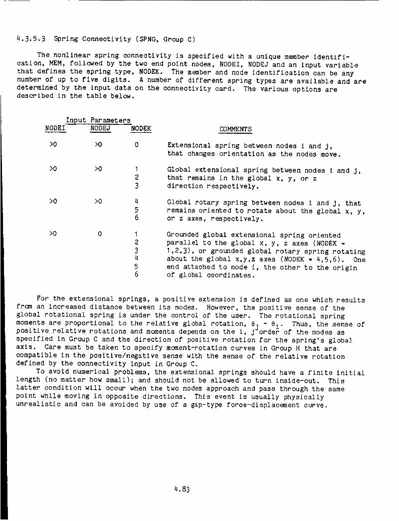
4.3.5.3 Spring Connectivity (SPNG,Group C)

The nonlinear spring connectivity is specified with a unique memberidentifi-cation, MEM,followed by the two end point nodes, NODEI,NODEJand an input variablethat defines the spring type, NODEK. The memberand node identification can be anynumber of up to five digits. A number of different spring types are available and aredetermined by the input data on the connectivity card. The various options aredescribed in the table below.

Input Parameters

NODEI NODEJ NODEK COMMENTS

>0 >0 0

>0 >0

>0 >0

>0 0 I

2

34

5

6

Extensional spring between nodes i and j,

that changes orientation as the nodes move.

Global extensional spring between nodes i and j,

that remains in the global x, y, or z

direction respectively.

Global rotary spring between nodes i and j, that

remains oriented to rotate about the global x, y,

or z axes, respectively.

Grounded global extensional spring oriented

parallel to the global x, y, z axes (NODEK =

1,2,3), or grounded global rotary spring rotating

about the global x,y,z axes (NODEK -- 4,5,6). One

end attached to node i, the other to the origin

o_" global coordinates.

For the extensional springs, a positive extension is defined as one which results

from an increased distance between its nodes. However, the positive sense of the

global rotational spring is under the control of the user. The rotational spring

moments are proportional to the relative global rotation, 8j - ei. Thus, the sense ofpositive relative rotations and moments depends on the i, J order of the nodes as

specified in Group C and the direction of positive rotation for the spring's globa]

axis. Care must be taken to specify moment-rotation curves in Group H that are

compatible in the positlve/negative sense with the sense of the relative rotation

defined by the connectivity input in Group C.

To avoid numerical problems, the extensional springs should have a finite initial

length (no matter how small); and should not be allowed to turn inside-out. This

latter condition will occur when the two nodes approach and pass through the same

point while moving in opposite directions. This event is usually physically

unrealistic and can be avoided by use of a gap-type force-displacement curve.

4.83

Example: Twotranslational springs in series

® ®

2I

0 ........ I ......... 2 ......... 3 ......... 4 ......... 5 ......... 6 ......... 7 ......... 8

123456789012345678901 2345678901 2345678901 2345678901 2345678901 2345678901 234567890

SPNG 3 I 2 0

SPNG 6 2 4 0

Example 2: Global translational spring in global x direction

1 2r X

0 ........ 1 ......... 2 ......... 3 ......... 4 ......... 5 ......... 6 ......... 7 ......... 8

123456789_123456789_123456789_123456789_123456789_123456789_123456789_123456789_

SPNG 10 I 2 I

Example 3: Torsional spring about the global x axis

0 ........ I......... 2 ......... 3 ......... 4 ......... 5 ......... 6 ......... 7 ......... 8

12345678901234567890123h56789012345678901234567890123456789012345678901 234567890

SPNG 5 I 2 4

4.3.5.4 Spring Stiffness Properties (PSPR, GroupH)

The spring stiffness properties are obtained as the slope of a multilinear forceversus elongation or momentversus rotation curves as shown in Fig. 4.3.7.

This table is specified in input Group H as input pairs of force (moment)andelongation (rotation). The necessary input for each table are:

NSPRG

USPRG

FAILT

FAILC

DMASS

FORCE

ELONG

The number of data points in the table; up to 20 pointsare allowed per table.

Slope used for unloading - optional.

Failure force in tension (+) - optional.

Failure force in compression (-) - optional.

Characteristic massused to compute the dampingcoefficient-optional.

Force (or moment)at the associated ELONG.

Relative elongation (or rotation) of the nodes at theassociated FORCE,uj - ui (or ej - ei).

If the elongation exceeds the last tabular input point, the last slope (either l-or 6-7 in Fig. 4.3.7) is continued until faille.

FORCE

7

4 I UNLOADINGRELOADINGSLOPE

ELONGATION

/1

Fig. 4.3.7 Force versus Elongation for Nonlinear Spring Element

4.85

The card input is in the following form;

CARDI contains the key word PSPRfollowed by the number of points in the table(NSPRG),the unloading slope, the failure force in tension and compression and thecharacteristic damping mass. A set of cards (of quantity = NSPRG)follow containingthe force, elongation pairs. The specification ends with a list of applicablemembers.

The input must be specified in the order of monotonic increasing elongation (fromnegative to positive values, as shownby the integers on Fig. 4.3.7). If it is not,an error messagewill be printed and the job will be aborted. In addition, one pairmust include the zero elongation point (not necessarily at zero force).

Note that the positive sense of the rotational springs are controlled by the userin the connectivity input Group C (Section 4.3.5.3 above). The curves input hereshould be compatible with the positive/negative sign convention as defined there, foreach rotary spring.

Unloading can occur in two waysr If the unloading slope has been input as zero(or blank) then the spring unloads along its original force-displacement path(conservative or elastic unload). If a finite slope has been input then unloadingoccurs along the linear path such as shown by the dotted line in Fig. 4.3.7.Subsequent reloading returns along the linear unloading slope, then rejoins andfollows the nonlinear curve. This element then has nonrecoverable or dissipativeenergy.

Positive and negative failure elongation (or rotation) can be specified, whichcauses deletion of element stiffness and force (or moment) as for other elements(Sect. 4.1.7), when these failure values are exceeded.

More complicated behavior can be developed by placing two or more nonlinearsprings in parallel or in series. However, take care to avoid massless nodes indynamic problems, or nodes without lateral restraint in static problems.

The damping force is proportional to, and opposes, the relative velocity of theelement's end nodes. The proportionality factor is not constant, but is dependent onthe current stiffness of the element, according to

C -- 2 / km (4.3.16)

where k is the absolute value of the current spring stiffness and m is a

characteristic mass (DMASS) specified in the input. Equation (4.3.16) represents the

critical damping factor for a one-degree of freedom system having the stiffness k and

mass m. Thus a part of the damping factor in a nonlinear spring element is set by the

user when specifying the characteristic mass DMASS in Group H, and a part is

controlled by the program in accordance with the changing element stiffness. This wasi

done to help control the behavior of gap elements, as discussed next. Damping is not i

operational with the explicit time integrators ADAM and CDIF. I

4.86

• _ FORCE

C

/f.A

D,_.

i'/;

E

j UNLOADI NGSLOPE

w

DISPLACEMENT

Fig. 4.3.8 Nominal Gap Spring Behavior

The nonlinear spring element can be used as a gap element to simulate the

kinematic constraints associated with contact and rebound such as occurs at impact

with external barriers or between parts of the structure. As shown in Fig 4.3.8, the

spring stiffness would change from zero in the gap region to a large stiffness to

simul_te a "rigid" contact. This stiffness should be in the order of magnitude of 10 2

or 10_ times greater than the effective structural stiffness at the contact node, to

be sufficiently "rigid" but still not too stiff to cause certain numerical problems.

However, using a sudden change in stiffness can still cause dynamic difficulties. In

Fig 4.3.8, it can be seen that as the gap is closed, the spring displacement proceeds

in one time step from point A to point B. At the end of that step, the spring force

is found to be at point C. If the spring stiffness and the displacement increment are

large enough, an unrealistically large force could suddenly be imposed on the

structure. This arbitrarily large force could cause false failures in the surrounding

structure and could result in the rapid repulsion of the spring nodes from each other

back into the gap zone. In many problems, the nodes may then be returned toward each

other again by external forces or inertias. This can result In a series of rapid

repeated contacts and rebounds, that can cause numerical difficulties, and is notrealistic.

A procedure that usually works well to prevent this problem, is to increase the

stiffness from zero by increments over a small distance, with large damping. This

will allow the spring force to increase to a more realistic value without overshoot,

and prevent the artificial contact-rebound oscillations, while allowing the spring to

rebound back into the gap region under the action of steady external tension forces.

This has worked well for simulating the impact and subsequent rebound of structures

with rigid barriers and with other moving bodies. The procedure is as follows (seeFlg 4.3.9):

4.87

I. Estimate the largest possible displacement increment imposed on the spring bythe impact speed and the time step at the instant of gap closure. This can beeasily done in most cases, by using the product of the initial impa_t speedand the maximumallowed time step (for example; 14 m/sec x 50 x 10-_ sec =7 x I0-4m = 0.7ram, therefore use I ram).

2. Define the value of the "rigid" barrier stiffness at 102 to _03stiffness of the surrounding structure (10 -10 lb/in, or 10 -10 -Imes_

the

Newtons/meter have worked well for "rigid" stiffnesses in some autos and

aircraft in past cases).

3. Increase the s_iffn_ss f_om z_ro to the "rigid" value in 3 or 4 jumps (forexample; 0, 10 _, 10", 10 _, 10 > N/m as in Fig. 4.3.9). Use the displacement

increment found in step I above for each segment to insure that at least one

point on each stiffness segment will be used.

4. Specify large damping by using a damping mass (DMASS) that is very large

compared to the effective mass at the spring nodes (100 times will usually

work well). If one node is fixed, then use the mass of the movable node as

the effective mass. If both are movable, use the smaller of the two as the

effective mass.

t Do not use an unloading slope (set USPRG--O). The spring will then be

nonlinearly elastic and will not permanently dissipate energy.

_FORCE

ACTU A L

_ "q--'-_ GAP, Au0---'---_

STIFFNESS '-109 N/M

7ID

DISPLACEMENT

FORCE,POINT N

1 -1062 -105

3 -104

4 -103

5 0

6 0

7 0

DISPLACEMENT,

M

-(Au 0 + .002)

-(AU 0 + .001 )

- AU 0-(AU 0 - .001 )

-(Au 0 - .002)01

Fig 4.3.9 Gap Spring Boundary Layer Example

4.88

In this method, the "rigid" barrier will usually be penetrated someacceptablesmall distance and the spring compression will respond smoothly to the external forceson it by increasing and decreasing in a controlled way. Note that, in Fig 4.3.9, theacutal barrier is in the middle of the boundary layer, which begins 2 mmbefore theactual gap is closed. This was done to minimize the penetration, but the user canplace the actual gap anywhere in the boundary layer with little error, assuming asmall boundary layer and a large gap.

The program also has a built-in procedure for controlling the contact/rebounddynamics, involving an automatic "capture" mechanism. This works by creating a"proportional band" around the gap closure point, and is activated simply byspecifying a finite unloading slope in step 5 above. The program will then create aproportional band of displacement width 2_ where _ is the initial penetration distanceDB in Fig. 4.3.8. The gap spring will unload from point C with a stiffness equal tothe unloading slope. Oscillations with damping will proceed between points C and E.Whenthe displacements would rebound past E, the force would drop to zero and the nodeis released to rebound freely into the gap zone, and it can return to start thecontact process once again. The proportional band 2_ is automatic and not under theuser's direct control. The unloading slope should be large (10_ N/m for the exampleused above), and the boundary layer (steps I-4 above) should still be used.

The preferred method is to use the boundary layer without the proportional band"capture" because the user has greater control over the contact behavior.

Example: a nonlinear crush spring with permanentdeformation (energy dissipation) incompression, and elastic in tension.

Given a table with 5 points for membersI through 10 and 53

FORCE ELONGATION

-I 000 -.2

-I 000 -. I

0.0 .0

1000 .I

2000 .2

Unloading slope is I x 104 (equal to the tension slope)

No failure criterion or damping

0 ........ I ......... 2 ......... 3 ......... 4 ......... 5 ......... 6 ......... 7 ......... 8

12345678901234567890123456789012345678901234567890123456789012345678901234567890PSPR 5.0 I.

PSPR -1000.0 -.2

PSPR -I000.0 -. I

PSPR 0.0 .0

PSPR I000.0 .I

PSPR 2000.0 .2

I -10 53

E+04 0.0 0.0 0.0

4.89

4.3.5.5 Loads (Group I)

The following mechanical loads may be applied to the spring element:

CONC- Concentrated forces applied at specified nodes in the global directions inthe units of force.

In addition, a table of the time distribution of the load, (load magnitude versustime), must be specified in the PTME,PTM2,or PTM3input in Group I.

These loads are discussed in Section 4.6

4.90

4.3.5.6 Description of Output o,

This section shows examples of typical output generated when using the spring

element.

Element Connectivity

SPRZNG ELEHENTSHEHBER NODE ! NODE J DZRECTION

901 133 12_ I902 133 126 I903 133 105 I905 133 100 I906 133 99 I907 133 97 1908 133 31 19_9 133 82 1910 133 96 1911 133 98 1912 133 26 1913 133 13 1914 133 45 1915 133 10 1916 133 95 1918 133 121 1919 133 132 I92B 133 122 1921 8 97922 78 132 1923 83 78924 113 114 3925 115 116 3

The values in the last column indicate the direction of global springs.

4.91

OIIUG_AL PAGE ISElement Stiffness Properties Clew _ QUAUTY

The example here Is an energy-dissipating crush spring with a varying force and a

maximum crush of 6.2 inches. The large unloading slope causes permanent deformation

with little spring-back. Damping must not be used when there is a negative slope as

in this case. A gap spring can be in parallel to also limit the crush.

APPLICABLE MEHRERS923

SPRING MATERIAL PROPERTY TABLE 4UNLOADING FAILURE FORCES

MODULUS TENS|ON COMPRESSION DAMP|NO MASS1.OOO0000E*06 e.eeoooooS.OO O.eOOeOOOE÷O0 O.OOOOOOOE+00

FORCE(MOMENT)-1.585000E÷_-'5.BSOOOOE÷O4-6.500000E*03-6.400000E-03-8.503000£_03-2.800000E_03"_.531000E_03-2.2BODO_E*03-4.600000E*03-7.589008E+03

e,eOOOOeE.q)O

DISPLACEMENT(ROTATION)-&.2OOeOOE÷O0"6.1OOO08E*OO"_.O00_OOE_e6-4.250000E_O0-3.628000E÷00-2.SOOO00E_O-1.750000E*00-1.150000E*O0-_.BOOOOOE-01-2.500000E-01

O.O000OOE*O0

NEHOER

901902q(_39059O69O79O891)991091!912912q14

916't18919q2Ot2)q22q23924')25

Force - Deflection Output

The output shown below is for a series of spring elements. The stiffness force

comes from the input curve of force vs displacement (or moment vs rotation), while the

damping force is calculated using Eq. 4.18 on p. 4.88. The Total force is the sum of

these two forces. The load state will be LOADING whenever the relative velocity of

its nodes is zero or is in the same direction as it experienced in the first time

increment, and UNLOADING when the velocity is in the opposite direction.

ELEMENT F_._I_E[_LIO_GAT|OII FOR NONLINEAR SPR|NG MEMBERSAT TIME - . ZNCR(NENT NUMBER • ql

ST|FFN£SS OANPIHG TOTALNOOE| NOOE J LOaD STATE FORCE

FORCE FORCE ELONGATION LENGTH

133 125 LOAOING O.O000000i,..o0 O.NOOOOOOE-RO 0.00000¢0(°00 -1,1_42330[-e0 1.07727k7[o01133 126 LOAOING O.ROOOOO0£*OO O.O000000E*eO 0.0000000[*00 -1.eS45435£-00 1.07724S7£-01133 105 LOADING |.O00OOOOE*OO e.eooooOOE-eO O.O0000OOE-eO -1,0&k5750[-00 1.07BO&25[*01233 100 LOAOING O.ROOOOOOE*I)O O.O00000DE*O0 O.OODOOOOE-eO -1.0511149E*00 1.0_STBE3E*01133 99 LOADING O.OOO0000I*OO |.OO00000[-O0 O.OOOOOOO[-.O0 -1.04_45k5[-00 l.OGb_543/*_l13$ 97 LOADING O.O00OO00[*O0 e.oooooDO[oO0 R.OOOOOOOE-.00 -1.050*163[*00 1.977&564[*01133 31 LOADING O.OOOOO00E-OO O.OOOOOOOE*00 |.O000000[-.OO -1.0,S0534E-00 1.07819,4£*e1133 12 LOADING O.OOOOO00E*OO R.OOOOOOOE*O0 O.O0000DO£*O0 -1.0,4423,£*00 1.0783577£oC1133 96 LOADING |.O000000E*.O0 R.OOOOOOOE-O0 O.O00OOOO£-O0 -1._S69256[,-00 1.177R07_[-01133 9R LOADING O.OOO0000£oO0 e.OOOO_OOS-O0 O.O000OOOi-OO -1.0407_k51-00 1.£7$&2&*EoOl133 26 LOADING |.OOOOO00[*OO O.OOODOOOE°00 O.O000OOOE*00 -1.0_33634E-00 I.g?S3637E-el133 13 LOADING |.oeooeoo£*O0 O.eooooocS-O© O.lo00000[oiO -l.o,o_o47[...oe 1.0786_q3£.,.01133 65 LOADING O.O000000E*Oe 9.eoooocoE-eo O.;ooooooE*eo -1.04942&q_-0o 1.0777573E_i]33 10 LOADING O.OOOOOOOE'_O0 O.OOOOO00E*O0 O,O000000E°t)O -1.O_O?6_E*O0 |.0702q2_,_133 95 LOADING O.OO00000E-OR o.eoooooOE-ee e.e_oooooE-oO -l.o_,7331E-ee 1.0772247E_133 121 LOADING -I.007_313E-02 -1._74291$E°03 -|.S7_0_48£-O3 mI.OO7SI13E-O2 5.94q92_7[,_1_133 132 LOAO;NG -|.3197B2_E*02 -|.5153**4E*03 -1.6473149E-03 -l.31q?O2_E-02 %.qSkB030[*O_

122 LOADING -|.2985O?kE*R2 *1.5_243_7E*03 -l.k_2*Oa&E*O3 -1.2985874[-'-02 _.q0701.1['t)013_ 97 LOADING O.O®OOOOOE*_O |.OOOOOOOE°OO R.OOOOOOOE..4O -2,ko7*elOE.-O3 2.qoS2393I*ex

7| 132 LOADING -6.9288&44£*03 O.OOoOOOOE*eO ,.4.92B8664_-03 -1.0195|iaE°O| &.|07.112I-_12 71 LOADING 4.8921q02£-t_2 I,ROO0000£°O0 6.|921902E*02 -1,008_Z74£-..02 S.2829111E,-O0

113 114 LOADING -I.4309397E-O2 R.ROOOODBE,-O0 -I.*IOq397E-02 -|.27339?9[.-04 1.t999873_.,.el_15 116 LOADING 2.9|9127&E-.01 R.O_OOOROE-tN) 2.9|91276E-,tl1 2.6_52457E-03 2.1N_26_SE.._I

4.92

4.3.6 Plate Bending Element - TRP2

4.3.6. I Introduction

TRP2 is a triangular plate bending element formulated for use in nonlinear

dynamics problems. The need for computational economy dominated the formulation of

this element in the sense that the "best" simplest element was sought. Numerical

evaluation has shown the TRP2 element to possess more than sufficient accuracy for

engineering computations, while its relative simplicity leads to less costly

computations. Nevertheless, it is still much more costly to use (from 9 to 27 times)

than a membrane triangular element. Consequently the user is advised to use membrane

elements to model for the essential features of the structural response wherever

possible.

In the derivation of this element the in-plane displacements, u and v are taken

to vary linearly. This leads to constant strain membrane behavior. The transverse

displacement, w, is cubic. For convenience transverse shear deformation is postulated

during the derivation. The rotations of the plate normal are given a quadratic

distribution throughout the element, and the transverse displacement is assumed to

vary quadratically along the edges. Additionally, the thin plate Kirchhoff hypotheses

are imposed at the vertices and at the midsides. These midside points are used only

as a convenience in the derivation and are not nodes in the final formulation. What

results from these discrete point Kirchhoff assumptions, and an additional assumption

on the rotation of the plate normal along the element edges, is an element in which

the Kirchhoff hypotheses hold along the edges as well as the vertices. In its final

formulation the TRP2 element is the three node triangular plate bending element shown

in Fig. (4.3.10). In global coordinates three translational and three rotational

degrees of freedom may be imposed at each node.

Fig. 4.3.10

Three Gauss integration points in the

plane, from three to nine Simpson

(including surfaces) integration

points throughout the element

thickness at each Gauss point.

Triangular Plate Element - TRP2

*See: H. Garnet and A.B. Pifko, "An Efficient Triangular Plate Bending Element For

Crash Simulation", in Advances and Trends In Structural and Solid Mechanics, Ed. by

A.K. Noor and J. Housner, Pergamon Press, New York, 1983, pp. 371-379 (Also

Computers& Structures vol. 16, No. I-4, pp. 371-379, 1983)

4.93

4.3.6.2 Input Data

The input data for the triangular bending elements TRP2are specified with thefollowing input cards:

Grou_ Keyword Required

C TRP2 Yes

H MATI Yes

H THIK Yes

CONC No

SURF No

Comments

Element identification and

connectivity.

This card type is used to

specify material properties.

Element thickness and number

of layers through the

thickness for Simpson's rule

integration.

Concentrated loads at nodes.

Distributed surface loads.

4.94

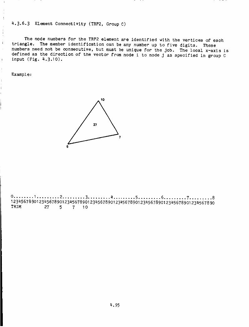
r

4.3.6.3 Element Connectivity (TRP2, Group C)

The node numbers for the TRP2 element are identified with the vertices of each

triangle. The member identification can be any number up to five digits. These

numbers need not be consecutive, but must be unique for the job. The local x-axis is

defined as the direction of the vector from node i to node j as specified in group C

input (Fig. 4.3.10).

Example:

Io

7

§

0 ........ I......... 2 ......... 3 ......... 4 ......... 5 ......... 6......... 7 ......... 8

123456789_123456789_123456789_123456789_123456789_123456789_123456789_123456789_

TRIM 27 5 7 10

4.95

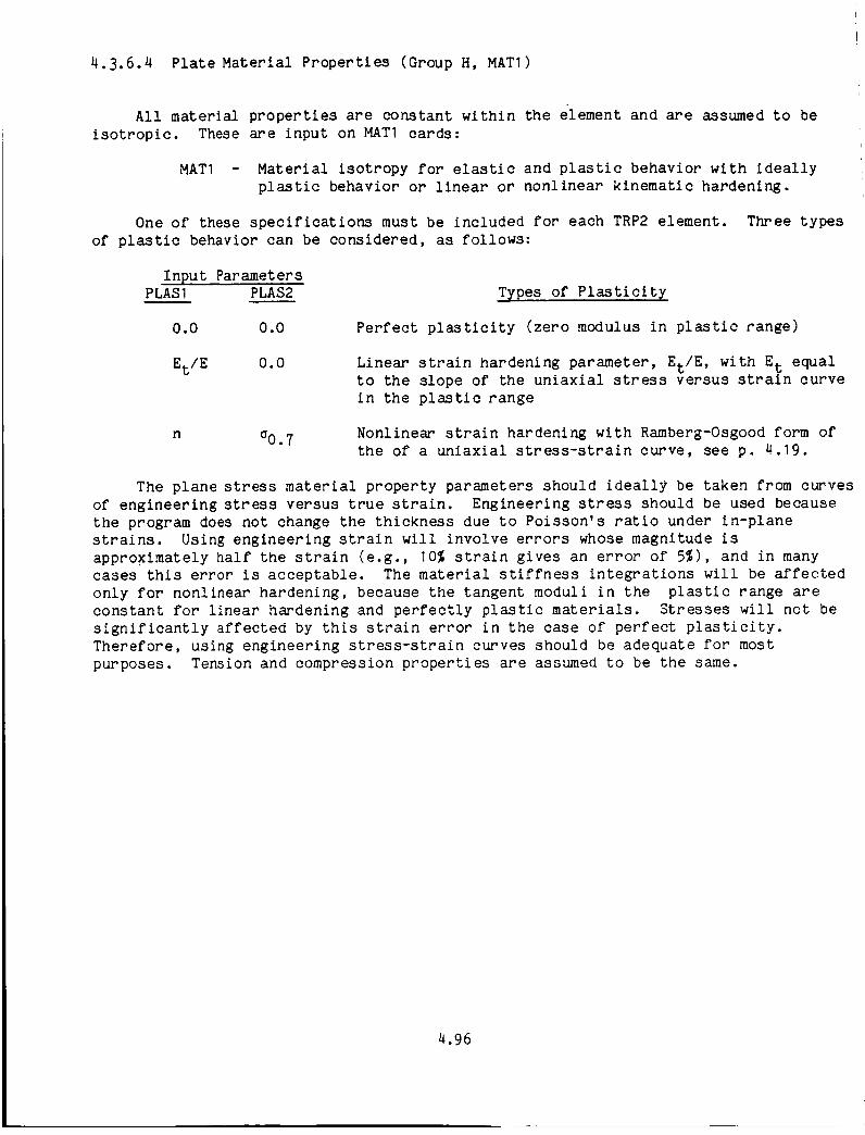
4.3.6.4 Plate Material Properties (Group H, MATI)

All material properties are constant within the element and are assumedto beisotropic. These are input on MATI cards:

MATI - Material isotropy for elastic and plastic behavior with ideallyplastic behavior or linear or nonlinear kinematic hardening.

One of these specifications must be included for each TRP2element. Three typesof plastic behavior can be considered, as follows:

Input ParametersPLASI PLAS2

0.0 0.0

Types of Plasticity

Perfect plasticity (zero modulus in plastic range)

Et/E 0.0 Linear strain hardening parameter, Et/E, with E t equal

to the slope of the uniaxial stress versus strain curve

in the plastic range

n _0.7 Nonlinear strain hardening with Ramberg-Osgood form of

the of a uniaxial stress-strain curve, see p. 4.19.

The plane stress material property parameters should ideally be taken from curves

of engineering stress versus true strain. Engineering stress should be used because

the program does not change the thickness due to Poisson's ratio under in-plane

strains. Using engineering strain will involve errors whose magnitude is

approximately half the strain (e.g., 10% strain gives an error of 5%), and in many

cases this error is acceptable. The material stiffness integrations will be affected

only for nonlinear hardening, because the tangent moduli in the plastic range are

constant for linear hardening and perfectly plastic materials. Stresses will not be

significantly affected by this strain error in the case of perfect plasticity.

Therefore, using engineering stress-strain curves should be adequate for most

purposes. Tension and compression properties are assumed to be the same.

4.96

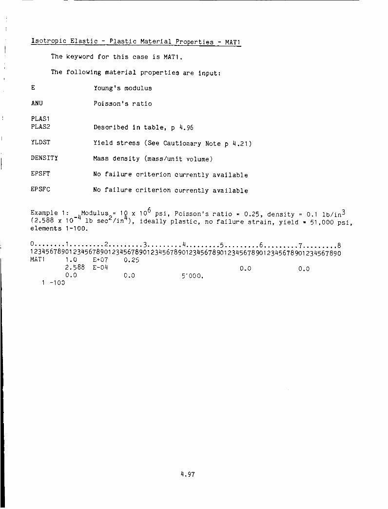
E

ANU

PLASI

PLAS2

YLDST

DENSITY

EPSFT

EPSFC

Isotropic Elastic - Plastic Material Properties - MATt

The keyword for this case is MATI.

The following material properties are input:

Young's modulus

Poisson's ratio

Described in table, p 4.96

Yield stress (See Cautionary Note p 4.21)

Mass density (mass/unit volume)

No failure criterion currently available

No failure criterion currently available

Example I- 4Modulus = 10 x 106 psi, Poisson's ratio = 0.25, density = 0.1 ib/in 3(2.588 x iO- ib sec2/in4), ideally plastic, no failure strain, yield = 51,000 psi,elements 1-100.

0 ........ I......... 2 ......... 3 ......... 4......... 5 ......... 6 ......... 7 ......... 8

123456789_123456789_123456789_123456789_123456789_123456789_123456789_123456789_

MATt 1.0 E÷07 0.25

2.588 E-04 0.0 0.0

0.0 0.0 51000.

I -100

4.97

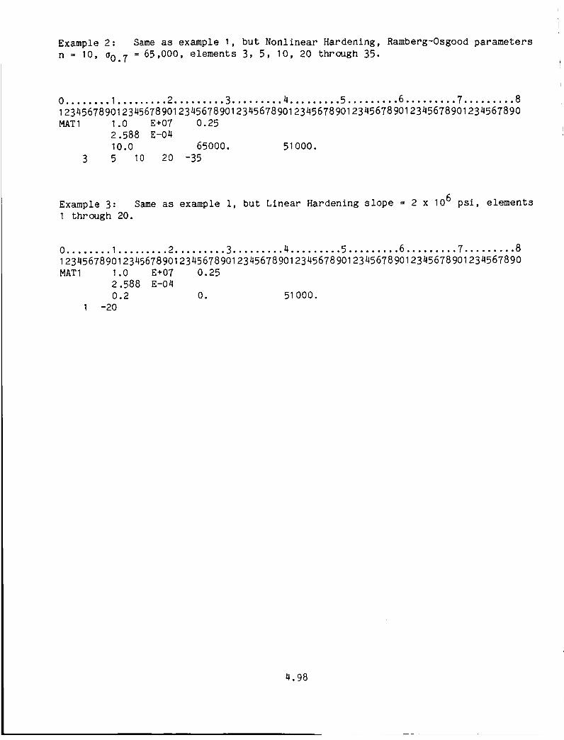
Example 2: Sameas example I, but Nonlinear Hardening, Ramberg-Osgoodparametersn - 10, _0.7 -- 65,000, elements 3, 5, 10, 20 through 35.

0........ I ......... 2 ......... 3......... 4......... 5 ......... 6 ......... 7......... 8123456789_123456789_123456789_123456789_123456789_123456789_123456789_123456789_MATI 1.0 E+07 0.25

2.588 E-0410.0 65000. 51000.

3 5 10 20 -35

Example 3: Sameas example i, but Linear Hardening slope = 2 x 106 psi, elements

I through 20.

0 ........ I ......... 2 ......... 3 ......... 4 ......... 5 ......... 6 ......... 7 ......... 8

12345678901234567890123456789012345678901234567890123456789012345678901234567890

MATI I .0 E+07 0.25

2.588 E-04

0.2 O. 51 000.

I -20

4.98

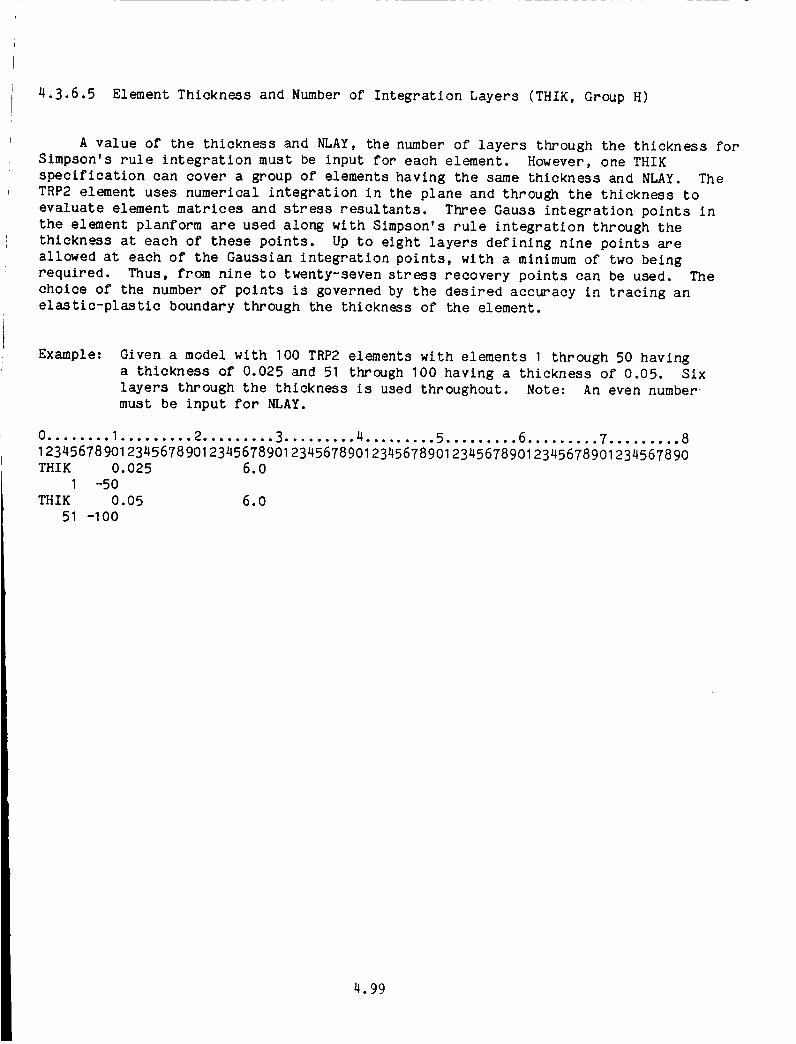
4.3.6.5 Element Thickness and Numberof Integration Layers (THIK, Group H)

A value of the thickness and NLAY,the number of layers through the thickness forSimpson's rule integration must be input for each element. However, one THIKspecification can cover a group of elements having the same thickness and NLAY. TheTRP2element uses numerical integration in the plane and through the thickness toevaluate element matrices and stress resultants. Three Gauss integration points inthe element planform are used along with Simpson's rule integration through thethickness at each of these points. Up to eight layers defining nine points areallowed at each of the Gaussian integration points, with a minimumof two beingrequired. Thus, from nine to twenty-seven stress recovery points can be used. Thechoice of the number of points is governed by the desired accuracy in tracing anelastic-plastic boundary through the thickness of the element.

Example: Given a model with 100 TRP2elements with elements I through 50 havinga thickness of 0.025 and 51 through 100 having a thickness of 0.05. Sixlayers through the thickness is used throughout. Note: An even numbermust be input for NLAY.

0........ I ......... 2......... 3......... 4......... 5......... 6......... 7......... 8123456789_123456789_123456789_123456789_123456789_123456789_123456789_123456789_THIK 0.025 6.0

I -5OTHIK 0.05 6.0

51 -IO0

4.99

4.3.6.6 Loads (Group I)

The following mechanical loads may be applied to the TRP2elements:

CONC- Concentrated forces and momentsapplied at specified nodes in the globaldirections in the units of force or force times length.

SURF- Distributed surface load on the element lateral surface. A linearvariation of the distributed load between nodes is assumed.

These are discussed in Section 4.6.

4.100

4.3.6.7 Output

ORIGr_!AL PAGE IS

OF POOR QUALITY

This section shows examples of typical output generated for the TRP2 element.

Element Connectivity.

TRIANGULAR PLATE ELEMENTS (TRP2)MEMBER NODE I. NODEJ NODE K

2B9 1BB 134 13121B 42 94 $6211 56 5S 42212 41 42 $5213 55 5* 41214 4¢ 41 $321S 53 41 54216 129 $3 52217 52 13B 129218 103 129 130219 130 1B4 103220 93 103 104221 104 17 93222 39 4B 103223 53 129 40224 129 103 4B225 44 131 134226 134 9"7227 1B3 93 39

Element Material Properties

APPLICABLE MEMBERS-86

NAT1HATERIAL PROPERTIES SPECZFICAT]ON TYPE 1YOUNG'S MODULUS POISSON RATIO PLAS1 PLAS2

3.0_00000E÷07 3.00000_0E41 1.382D_00E-_3 0.0_00E+00FAILURE STRAINYIELD STRESS DENSITY TENSION CONPRESg_ON2.3980000E'_4 7.3320000E-¢4 3.000_000E-01 -1._000000E+00

241 -256 271 -276

4.101

Element Thickness

APPLXCABLE MEMBERS1 -30

THICKNESS TYPE I ISTHE HUHBER OF LAYERS IS

Z.;?9OOOOD+O08

Stress and Strain Output

The output below is typical for each TRP2 element for which output is desired.

First are the local coordinates of three Gauss points (Fig 4.3.10), followed by the

plate stress resultants, Nx, N., Nz, M x, M., M x. and membrane strains and curvatures,y Je x, e., exy, kx, kv, kxv at each Gaussian _ntegratlon point. These data are followedby a _ist of each SimpsOn integration point through the thickness, including the top

and bottom surfaces at each Gauss point, with the ratio of the Von Mises stress to the

current effective yield stress, and a status indicator. A stress ratio less than one

indicates that the point is elastic having never been plastic, with an indicator of

NO, or elastically unloaded from a previous plastic state, indicated by UN. If a

point is plastic the indicator is YES. The upper and lower surface total strains and

stresses follow. If all the points in the element are elastic this completes the

output. If any point is or previously was plastic, the stresses and plastic strains

for each point follows, from the upper to the lower surface for the three Gauss points

in turn. In this particular example there are 8 layers so that there are a total of

27 stress points. (9 Simpson points through the thickness times 3 Gauss points along

the plane)

4.102

INT[G.POlN|

I2)

fNT[G.PO|N|

1)

INIEG.@QINT

I

ORIGINAL PAGE IS

OF JALn'y0VCAST EXARPL| P|OOL|m INPUtSlVELY tOA0(0 PLAT| CLAHP(O 11019611 (011282.Ptql PAG[ 117

STO|SS[S ANO 511lAIN5 F011 TI|AHGULA0 0tH01NG £L_MENT (TIIpZ[L)AT TIHt * $000000n-04 n[M9(l • I

TNICIN|5$C00eOINAY£ PLASTIC1.2495000,00 UH1.1712500-0i Utl6.ZG75OOO-01 UNS.1237100-01 UN0.0 UN

-3.1237500-01 UN-6._475000-01 UH-9.1712500-01 U*I-1.2491000*00 UN

LOCAL C0000|HAI|5 S T 9 _ S $ 0 £ S U L T • N Y 5 •• Y NX NY H)[Y HI( HV IqXY

4. 2424760,00 5.7892470-01 -4. 1088710.0t i.2049190*02 5.9406410,01 ?. 721•9T0,00 $. 7409t.20*0t I . 50tSOSD-01i.0747190*01 7.20&9200"00 -1 . 2505(IS0.02 -|.191C*Ti0*0Z -2. 3745080,0| 6.1466730,01 1.Z05730fl,02 -4.IkS56TO*011.0715050,0I 5. 78924;0*01 -J.5773150001 1. 3780310*01 $.2185000.01 1. 7713500*02 7.01t17400,01 -3.•0&)1&DOG1

N i tq J I A N ( S T | A IN C U I V & T U t E S[If [ Y ( XV [AP- X KAP-Y i| AP- Xy

| .$90|480-0_ 4.2811310-07 -_. 27024;,80-03 I . 3448170-01 2. 3441 _00-02 I • 291_" 340-0_,I*59014&O°OZ 4.28171|0-02 -4.Z?02480-03 3.4104560-04 2.ZZ $J9C*D-02 -3.0|81350-05J .S$01480-02 6.2017310-02 -4.2T02400-03 5.0991120-04 2. $479660-02 -3.6070790*05

FIIACT ION INT[G. FIACTI0N |HT[G. TOACTIONOF Y|(t0 5TI1(55 POINf PLASTIC OI r YI£LO STILE55 POINT PLASTIC OF YI(L0 STOE55

I. 1975830-01 2 UH 7. t 94S870-01 ) UN 4. 261063D-016.8488040°0 J UH &. ZASTBID-0t UN 4. 70441,60-0|2.9538230"01 UN 7.7376410-01 UIl 1.4374_, t rt-Ol3.9 ? I 1420- 01 UH T. 5958250-01 UN 2.3791.0 SO*0 I8.6040310-01 UN &.6040|10-01 UN 8.&0401tDo01?. 7859000-01 uH 8.6587780-01 uN &.06t9940-013. S) 70929 -01 UH 0. &709420-0 I UN 6 * 56'_-• 870-0 IS. 5783860-01 UN 4.5818co 70" 0 I UN 6 • •A44610-O I5.3094390-01 Utl 5.5433340-0i UN 7.110;$920o0L

S T O E 5 S • N 0 TOTAL S T 0 A I N A T U P P | 0 5 U t f A C I_|OT-X IOT-Y TQ[-XY 51G-X 5IG*Y $1G-XY

I . T584380-02 7.211T_I0-0_ -4.1084000-03 11.7314470,01 1.2814&;0*02 1.0918190,011.63ZF&ZO-02 7.0191120-02 -4. J079600-03 6.2312400,0i 2. _478780,02 -4.2454700.01| .6138660-02 ?.21_Si40-02 -4.$128190-01 I .A076320*02 I. $441810.02 -3.2480460*00

S T t [ S 5 • N 0 I 0 T A t 5 T II & | H AT L 0 N [ l 5 U t I: A C i

IHI|G.POINT

IZ3

INT[G.POfH!

I2)

5T0_$5 POINT1" It- 2t- 3I- 4I* SJ- 6l* 7t- 8I- 9_* IZ" ZZ- 3

2- S2- 6Z* 7Z- 8

2- q))- |

)- $

I- S)- 6)- ?J- 8)- 9

TOT-X lO|-¥ IOT-xY 51G-X 5IG-Y SIG-XY1.4218580-02 1.3117410-02 *4.4320879-03 -6.1711700*00 1.259t910*02 1.4645110,011.5415140-02 I.S0381iO-02 -4.2521160-03 -11.5507380,01 1.47_1840*01 2.546590n*01).5244]00-02 1.3_71400-02 *4.2276/&U°03 -I.0365700.02 11.8174190*01 2.18411_00,01

STt[S5 PLASTIC 5|lAINPtAS|IC SIG°K 51G-v SIG-_V [PS-X |PS-V EPS-XY

UN 9.2354470*01 1.20t4670*02 1.09_6190*01 |.7323940-02 7.1611990-02 *_.2411q60003UN -4.&T&1)YIO*01 1.6517860.02 1.2_041_O,01 1.7678qt0-02 6.$926730-02 -4.3021579-03UN 1.8001160'00 9.8J)1800*01 1.1_823_0"01 t.&876710-02 S.&9_4830"02 "4.3122910-03UN 1.3838180*01 4.05_|700*0! 4.SOt&7_G*0l |.6314120-0_ 4.9q66440-02 -4.8072/40-03UN -6.0_74710,01 -I.29743_0,0_ 5.56117860,01 I.&O06JZD*02 4.))$4010-02 -4.9&T8140-03UN -4.171171170,0l -I.4|70100,_ I.TA087UO*Ut |.S474410-02 J.O|_S?00-OZ -4.5544880-01UN -9.3593110,00 9.0252170*01 I.$tl)_I0,0I 1.$23•050-02 2.7717800°02 -4.51588)0-01UN -i,14SIO00*OI 1.5_11129._2 1.0193090.01 1,4000990-02 2.0177910-02 -4.6_01100-03UIi -&.1711700,00 I.ZS_$SO*OZ I*k6_SJiO*Oi 1.4_1i000-02 1.2099700*02 -4.64|1190-0_Ull 6.2512400.0i Z.14107_0.02 -4.2634T00.01 I.&$_5050-07 6.9451160-02 -3.7722000-0_Uil -1.176627U*01 t.Aiq&;S0.0Z -5.038Z100.01 i.&_83_70-02 6.29481_0-02 -3.$&52200-01U0i 04.4;71060,01 -5.707_530,01 -7.i0471_0001 |.&_A&500-0Z 5.69_1410°02 o3.3865710-03UN *l.1466400,01 -I.1830)70002 -I.710|40U*01 I.SSOI&IO-OZ S.0)14010-02 o4.0440110-03Uli -6.047_710,01 -I,29_150'02 _.5697_60*Ot |.k004|20-02 4._15_0J0-0_ -4.9&90140-03

Uli -8.24976_0"01 -1.801_1_1)*02 -6.O_J]OU*OO 1._82_97_-02 _.t461200-02 *_.1741570-03UN 00.117_550,01 -3.0710900"01 _.0003_20"00 I.S94_990-02 Z.20|00£0-02 0_.3230_10-03

UN *9.510_380'|I 1.4731840001 2.5665980"01 |.51156080-02 I._828920"02 °4.55231)80-03UN 1.00763_0*02 1.34_|810*02 -3._480460*00 1.5860220-02 7 1767750°02 -4._T20_30-03UN 1.393q170,07 1.95_8460.0_ -4.090&SAG,Q1 1.Sq87170-02 6.4005180-02 -3.7873720-03UH 9.4251450.01 11.ASqAlq0*01 -9.24_8740,00 |.Sq01840-0_ 5.7145050*02 °4.17518q0-03UN 3.3370100,01 2.5q0ZO_O*0i 1._018170'01 |.5937110-02 S.0071000-02 -4.4691100-03UH -4.047_710,01 -I.2924110.0_ 5.5697060*01 |.&OO&$_O-02 4.)_$4030-02 -4.96903_0-05UN -7.93477_0,01 *l.&780&|0*0_ ).0011150,01 1.5001_80-02 3.6|78_0-02 -4.64688i0-03UN -9.6991740,01 5.96_0020*0| _.04011_O*01 I.&1J7890-02 _.77|9T|D*02 -_.6014110-03UN -I.1871420'02 1.02_17_0,0_ ).01|7960,OI |.&1417_0-07 7.016•970-02 -_.6|93i10-G)UN -I.0165700"07 9.&874i90"0i 2i009q00"0i i.5907_D-0_ 1*281_980"02 "_.SOZ£IJ_-O]

4.103

4.3.7 Contact Element - GRDS

4.3.7.1 Introduction

The contact element is a nonlinear spring element that is used for contact

between any node and a prescribed fixed contact plane. It is similar to the "gap"

capability available with the nonlinear spring element but has a number of additional

features. These are;

o The initial gap distance between the contact node and contact plane is

calculated automatically.

o The contact plane can be skewed with respect to the global system without the

necessity to use multi-point constraint conditions.

o Sliding friction forces between the contact node and contact plane are

included.

o User input contact and rebound tolerances can control the contact and rebound.

4.104

4.3.7.2 Contact Element Input Data

The data for the ground contact element are specified with the following cards:

Grou_ Keyword Required

C GRDS Yes

H PGRD Yeso

Comments

Element identification

and connectivity.

Element properties

including contact plane

definition.

4.105

4.3.7.3. Contact Element Connectivity (GRDS,Group C)

A separate ground contact element is defined from each contact node to a fixedcontact plane. The contact element connectivity is specified with a unique memberidentification (MEM)followed by the contact node number (NODE)and an identifier(NDIR) that defines the global axis which is closest to the normal to the contactplane. The NDIRcan be I, 2, or 3 denoting the global X, Y, or Z directions. Thememberand node identification can be any number of up to five digits.

The use of the direction identifier NDIRcan be demonstrated for the case ofcontact with the ground which is parallel to the global X, Y plane and whose normal isparallel to the global Z axis. Then NDIR = 3, denoting that the contact plane's

normal is closest to the global Z direction. For the case of contact with a global Y,

Z plane, NDIR = I. Note that the contact plane does not have to be exactly normal to

the NDIR direction, that more than one contact plane is allowed, and that one node can

have more than one GRDS element to contact more then one surface.

4.106

Example: Mass impacting two constraint planes

fJfI_'fffif_ rl/IIIIIIIIIIIIIIIIlttIIIIII_ rf f

×

0 ........ I ........ 2 ......... 3 ......... 4 ......... 5 ......... 6 ......... 7 ......... 8

1 2345678901 2345678901 2345678901 23456789012345678901 2345678901 2345678901 234567890

GRDS I I 3

GRDS 2 I I

NOTE: Additional input (GRDS) is required to define the contact plane in Group H.

4.1 07

4.3.7.4 Contact Element Properties (PGRD,Group H)

The properties for the contact element include a multilinear force versusdisplacement table, three points defining the contact plane, and a numberofparameters.

The input parameters on the PGRDcards are summarizedbelow:

NSPRG

FRICT

EPSC

EPSR

DMASS

COORD

FORCE

ELONG

The numberof force-displacement points

Coefficient of sliding friction

Contact tolerance

Reboundtolerance

Characteristic mass used to compute thedamping coefficient

Coordinates of three points on the contact plane

Contact force

Contact displacement (penetration).

4.108

The contact plane is defined by three points denoted by i, j, k in fig. 4.3.11.The order in which the coordinates (COORD)of these points are given define a righthand local coordinate system, X', Y', Z' in the following manner: The direction i - jdefines the X' axis, Y' starts from point i and is parallel to the normal vector fromthe X' axis to point k, and Z' is perpendicular to the X', Y' plane. At the initia_time t=0, the contact node must _e either touching the plane or be above it, i.e. Z0 >0. Since the direction of the Z axis is determined by the order of the nodes i, J,k, the user must determine on which side of the contact plane is the structure, andspecify nodes i, j, k in the proDer sequence.

CONTACT

z' NODE

CONTACT ELEMENT

i 7" ..... -.D=,. y'

Fig. 4.3.11 Contact Plane Definition

4.109

The usual contact rebound sequence is as follows: The gap distance Z' willdecrease to zero as contact occurs, then becomenegative as the contact nodepenetrates slightly into the surface while the contact force builds up, and eventuallythe contact node mayrebound off the surface. The contact forces will vary asrequired by the action of the remaining structure on the contact node. The nodalmotion normal to the surface is controlled by a user specified curve of contact forcevs. penetration distance and by damping which is partly under user control. The nodalmotion tangential to the surface produces a friction force with a user-specifiedfriction coeffecient. The node can rebound off the surface, and there is no limit tothe number of contact-rebounds.

The contact criterion is defined as:

Z' > O, no contactZ' < O, contact.

Initially as long as Z' > 0 the contact spring has zero force and stiffness.WhenZ' < 0 a user-specified curve of compression force vs. penetration distanceis used.-- The contact spring stiffness must be in the order of magnitude of 10_ to 103times greater than the effective structural stiffness at the contact node, to simulatea "rigid" barrier without numerical problems. However, if the large stiffness wereimposed suddenly, and there were no special control on the time step, then a largedisplacement increment together with the large stiffness could place anunrealistically large force on the contact node. This large force could result in therapid repulsion of the contact node back into the structure causing false failures.In somecases, the contact node can be returned rapidly into the contact surface againby the structure, resulting in a series of rapid repeated contacts and rebounds, whichare not real and can cause numerical difficulties.

Several procedures are used to control the contact-rebound behavior. Theseinclude: incremental stiffening, damping, displacement increment control, and reboundcapture. With these features, the contact force can increase to a realistic valuewithout overshoot, without artificial contact-rebound oscillations, and then thecontact node can be pulled away from the barrier surface by the steady rebound motionof the structure. Dampingis not operational with the explicit time integrators ADAMand CDIF.

4.110

A typical contact spring curve with incremental stiffening is shown in Fig.4.3.12. The stiffness is increased from zero to its "rigid" barrier value byincrements over a small distance (a "boundary layer"). This boundary layer is madesmall relative to the gross structural deformation (4 mmis used in the example ofFig. 4.3.12).

As the contact node initally approaches the contact plane, the penetrationd : -Z' is negative and the contact force is zero. After penetration d > O, and theforce rises smoothly and steadily over a small penetration distance, from points I to2 to 3 etc., until the contact force is in dynamic equilibrium with the structural andinertial forces acting on the contact node. The contact force and penetration willvary as the impact event continues, depending on the behavior of the structureattached to the node, and additionally upon the damping characteristics of the contactspring.

CONTACT

FORCE, f

COMPRESSION

STIFFNESS

== 10= N/m

PENETRATION DISTANCE

d == -z'

"FORCE," f "ELONG," d

POINT (NEWTON) (METER)

1 0 0

2 10= .001

3 10= .002

4 10' .003

5 10= .004

_c = 2ram

c r = 1turn

Fig. 4.3.12 Contact Spring Boundary Layer Example

4.111

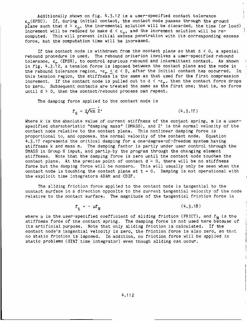
Additionally shownon fig. 4.3.12 is a user-specified contact toleranceCc(EPSC). If, during initial contact, the contact node passes through the groundplane such that d > cc, the incremental solution will be discarded, the time (or load)increment will be reduced to maked < _c' and the increment solution will be re-computed. This will prevent initial excess penetration with its corresponding excessforce, but the computation time will be increased.

If the contact node is withdrawn from the contact plane so that d < O, a specialrebound procedure is used. The rebound criterion involves a user-specified reboundtolerance, Cr (EPSR), to control spurious rebound and intermittant contact. As shownin fig. 4.3.12, a tension force is imposed between the contact plane and the node inthe rebound tolerance region, -_r < d < O, after the initial contact has occurred. Inthis tension region, the stiffness is the sameas that used for the first compressionincrement. If the contact node is pulled out to d < -¢r' then the contact force dropsto zero. Subsequent contacts are treated the sameas the first one; that is, no forceuntil d > O, then the contact/rebound process can repeat.

The damping force applied to the contact node is

fd -- _/km Z' (4.3.17)

Wherek is the absolute value of current stiffness of the contact spring, m is a user-specified characteristic "damping mass" (DMASS),and Z' is the normal velocity of thecontact node relative to the contact plane. This nonlinear damping force isproportional to, and opposes, the normal velocity of the contact node. Equation4.3.17 represents the critical damping for a one-degree-of-freedom system havingstiffness k and mass m. The damping factor is partly under user control through theDMASSin Group H input, and partly, by the program through the changing elementstiffness. Note that the damping force is zero until the contact node touches thecontact plane. At the precise point of contact d -- O, there will be no stiffnessforce but the damping force will be nonzero. This will usually only be seen when thecontact node is touching the contact plane at t -- 0. Damping is not operational withthe explicit time integrators ADAMand CDIF.

The sliding friction force applied to the contact node is tangential to thecontact surface in a direction opposite to the current tangential velocity of the noderelative to the contact surface. The magnitude of the tangential friction force is

ft = - _fN (4.3.18)

where _ is the user-specified coefficient of sliding friction (FRICT), and fN is thestiffness force of the contact spring. The damping force is not used here because ofits artificial purpose. Note that only sliding friction is calculated. If thecontact node's tangential velocity is zero, the friction force is also zero, so theftno static friction is imposed. In addition, no friction force will be applied _nstatic problems (STATtime integrator) even though sliding can occur.

4.112

The recommendedprocedure for preparing the input for the contact element'sproperties on the PGRDcards of Group H is as follows:

I . Estimate the largest possible displacement increment imposed on the spring by

the impact speed and the time step at the instant of gap closure. This can

be easily done in most cases, by using the product of the initial impactspeed and the. maximum allowed time step (for example; 14 m/sec x 50 x 10 -v

sec : 7 x I0-4m : 0.Tram, therefore use I ram).

m

Define the value of the "rigid" barrier stiffness at 102 to 403 _imes thestiffness of the surrounding structure (10 -107 ib/in, or I0_-I0 _

Newtons/meter have worked well for "rigid" stiffness in some autos and

aircraft in past cases).

.

Increase the s_iffn_ss f_om z_ro to the "rigid" value in 3 or 4 jumps (forexample; 0, 10 , I0", 10v, I0 J N/m as in Fig. 4.3.12). Use the displacement

increment found in step I above for each segment to insure that at least one

point on each stiffness segment will be used. The FORCE-ELONG input pairs ofFig. 4.3.12 were chosen for convenience rather than exactness.

. Choose a contact tolerance EPSC that is larger than the displacement

increment calculated for step I above. This should allow the "boundary

layer" stiffness forces to increase properly without reducing the time

step. The contact tolerance then becomes an upper limit control, which will

protect against unexpectedly large increments, but at the price of

temporarily reducing the time step. (For the example, 2mm would be used).

. The rebound tolerance EPSR might be in the range between zero and the contact

tolerance value (EPSC). Try using a value equal to the displacement

increment calculated in step I, until greater experience is gained.

. Specify large damping by using a damping mass (DMASS) that is very large

compared to the effective mass at the contact nodes (from 10 to 100 times

will usually work well).

With these values, the "rigid" barrier plane will usually be penetrated some

acceptably small distance into its "boundary layer", and the contact force will

respond by increasing and decreasing in a smooth, controlled manner between reasonable

limits, until the structure rebounds. Note that the damping is not operational with

the explicit time integrator ADAM and CDIF.

It will be noted that this PGRD input for the ground contact spring element GRDS

is similar to that of the PSPR input for the general purpose nonlinear spring SPNG

when used as a gap spring. The ground contact spring is a more recent development

which provides an enhanced contact capability, yet reduces the amount of input data.

The user does not specify the initial gap distance from the node to the contact

surface because the program calculates it. Once a contact surface's properties have

been defined in one PGRD card set, it can be assigned to any number of contact nodes

having varying gap distances. Therefore, a large number of gap spring property card

sets are not needed with the ground contact springs. Usually, only one such carU set

is required. In contrast, the general purpose gap spring requires a separate PSPR

card set for each different gap distance.

4.113

The card input is in the following form; CARDI contains the key word PCONfollowed by the numberof force-displacement paints (NSPRG),the friction coefficient(FRICT), the contact tolerance (EPSC), rebound tolerance (EPSR), and the damping mass(DMASS). The next three cards each contain the global coordinates of point on thecontact plane. The order of their input determines the direction of the outwardpointing normal to the contact node. This normal should always be on the sameside ofthe plane as the contact node. The succeeding cards are the force (FORCE)versusdisplacement (ELONG)pairs. Thesemust start at 0,0 and must be always positive. TheELONGvalues must increase monotonically, but the FORCEvalues can vary arbitrarily.The PGRDcard set ends with a list of the identification numbers for the applicableGRDSmembers.

Example:

Contact on a plane whoseperpendicular is in the global Z direction.

The following parameters are specified: Coefficient of friction _ = .3,Contact/rebound tolerances e c = .10, Er .05 , damping-mass m 10.

Z

The three points defining the contact plane are:

Point X Y Z

i

i 0.0 0.0 I .0

j 0.0 10.0 I .0 /k -I 0.0 0.0 I .0

z' _y °

y

Five points are used to defined the contact force versus penetration displacement

curve.

Force Displacement

0.0 0.0

.5 x 102 .05

.5 x 103 .10

.5 x 104 .15

•5 x 105 .20

(These are the pound and inch

approximations of the boundary

layer example in Fig. 4.3.12, p. 4.1_I.

It ends in a "rigid" stiffness of 10_

lb/in.)

The data is applicable for GRDS members 101 and 102.

4.114

0....... I ......... 2......... 3......... 4......... 5......... 6......... 7......... 812345678901234567890123456789012345678901234567890123456789012345678901234567890

PGRD 5.0 • 30.0 0.00.0 10.0

-I 0.0 0.0

0.0 0.0

0.5 E+02 0.05

O. 5 E+03 O. I0

0.5 E+04 O. 15

O. 5 E+O 5 O. 20

101 102

0.10

1.0

1.0

1.0

0.05 10.

4.3.7.5 Contact Element Loads (Group I)

CONC - Concentrated forces applied at specified contact nodes in the globaldirections in units of force.

In addition, a table of the variation of the load magnitude versus time must be

specified in the input of Group I. CONC is discussed in Section 4.6.

4.3.7.6 Contact Element Output

This section shows examples of typical output generated when using the contact

spring element.

Contact Element Connectivity

r_OO'E'D COIE'TACT ELICIT5

NODE DI]LZCTION

202 701 3 "103 703 $

Contact Element Stiffness Properties

APPLI CA]SLE 14ZKSEES

I01 102

C20171iD CONTACT ZLEMEET PEOPZET_ TAJSLE 1FZlCTIOII DAMPING

COEEF ICI ENT MASS

3. 00000OOE'O2 2.0OOOOO01[,01

COOEDINATZS OF (20031D CONTACT PLANEX ¥ Z

O.O0000OOE*O0 O.OOO00OOE*OO 1.OOOOOOOE',O0O.0000000E*O0 1.0000000E*01 1.00OOOO01',00

"l.0000000E_'Ol O.0000OOOE*OO l. OOOOO00EtOOEOZCZ ELONGATION

O. 000000E*OG O. 000000][, O0S. O00000E*OI 5. O00000E-025. O00000E*03 1. O00000E-015. 000000E *03 1. 5000001' -015. 000000E,04 2. O000OOE-01

4.115

Contact Element Output

The output shown below are for two different cases, one before contact and one

after contact. Contact is indicated in the appropriate column with a YES or NO. The

"Closest global axis" indicates that the normal to the plane is specified to be

closest to one of the global XYZ directions indicated by a I, 2, or 3 respectively.

The friction force components are tangent to the contact plane and in the contact

plane's local coordinate system, defined earlier in Section 4.3.7.4 and Fig. 4.3.11.

The "distance from plane" is the value of Z'. A positive value is the gap

distance from the node to the plane before contact, and a negative value is the

penetration after contact. Note that the input penetration distance d has the

opposite sign.

The stiffness and damping forces are added to produce the total normal force.

Normal forces are positive for tension (pulling the node into deeper penetration) and

negative for compression (pushing the node out). The signs of the stiffness force and

distance from plane should always agree.

The total friction force (vector sum) is equal to the friction coefficient times

the normal stiffness force.

FORCES AND CONTACT COND]T;ON FOR GROUND CONTACT ELEMENTS AT TIME - 6.5B8088E,-O1

CLOSES? FRiCTJON FORCE_ NORMAL _ORCES DTSTANC_MEMUEk NOD[ GLOEA; AXIS CONTACT LOCAL ) LOC_, _ 5TIFFNES_ DAHF;NC TO1AL FROM PLAN[

1C2 7_1 3 NO _.BOD_-DC £.BOOE+BC O.BOOE+O_ C.DOOF÷B_ C.OO¢E÷0¢ 5.0OOE-B_1C; 702 3 NO B.B_8E.t.O_ E.OBGE*O_ O.OBOE_B_ _.D_OE'.'O£ O.BOOE+BO 5.BOOE-B_

FORCES AND CONTACT CONDITION FOR GROUND CONTACT ELEMENTS AT TIME o B.158800E+BO

CLOSEST FRICT]ON FORCES NORMAL FORCES D|STANCEMEMBE_ NODE GLOBAL AXIS CONTACT LOCAL X LOCAL Y STIFFNESS DAMPING TOTAL FROt4 PLANE

101 701 3 YES -1.295E÷00 1.295E÷t_ -6.106E'_00 3.152E't'00 -2.953E÷B¢ -6.11_E"e3102 702 3 YES -1.3_.E','1_ 1.31_E'q_ --_.166E_i_ 1.9,1E_-I_ -_.2Bk£÷BB -6.1_E'-03

4.116

4.4 NODALCOORDINATES(GROUPD, GRDX,GRDY,GRDZ)

Nodal coordinates are specified in a global XYZcoordinate system. Coordinatesare input using three key words, GRDX,GRDY,GRDZfor the coordinates in the X,Y,Zdirections respectively. Each input card of this type contains one of the above keywords to specify the component, the coordinate location, and the applicable nodes.All the short form notations can be used to specify applicable nodes, i.e., I through100 and 2, 4, 6 ... 100 becomes1-100 and 2-2-100, respectively.

Example: An X coordinate of 20 is specified for nodes I through I0, 14, 20, 23, 26,49, 54, 57, 37, 39, 40 and 101, 103 ... 121.

0........ I ......... 2 ......... 3......... 4......... 5 ......... 6......... 7 ......... 812345678901234567890123456789012345678901234567890123456789012345678901234567890GRDX 20.0 I -I0 I 4 20 23 26 49 54 57 37 39 40GRDX 101 -2 -121

The coordinate 20.0 need not be input on the continuation card since these fieldsare ignored. Any number of continuation cards can be used with one blank I5 fieldending the input for the coordinate. If the applicable nodes fill up the card, i.e.,end on the last I5 field, then an additional continuation card must be input with thefirst I5 field blank.

4.1 17

4.4.1 Vehicle and Global Coordinate Systems (XSHF, YSHF, ZSHF,YAW,PITC, ROLL

While it is usual to use a single fixed global coordinate system for specifyingthe initial nodal locations, it can sometimes be better to specify the initialcoordinates in a more convenient second system and then specify the position of thesecond system relative to the global system. This second coordinate system will becalled the vehicle coordinate system, and will be useful in cases where the initialcoordinates of the vehicle or structure are already known in the vehicle system whichis displaced and rotated with respect to the global system fixed to the impactsurface. This is even more useful when the vehicle will be given several differentinitial positions relative to the impact surface. In each case, the samenodalcoordinates can be used in the vehicle coordinate system, while different initialpositions are specified for the vehicle system relative to the global system. DYCASTwill internally transform the initial vehicle coordinates into the initial globalcoordinates, which DYCASTwill use for all subsequent calculations.

Therefore, use of any of the parameters XSHF, YSHF,ZSHF, YAW,PITC, and ROLLininput group D, will cause the initial coordinate transformation to be implemented, andthe nodal coordinates input using GRDX,GRDY,GRDZ,must then be in the vehiclecoordinate system. Values of XSHF,YSHF,and ZSHFwill shift the origin of thevehicle coordinate system by the specified distances from the global system origin inthe global X, Y, and Z directions. The vehicle coordinate system will be rotatedrelative to the global coordinate system according to the angles given by theparameters YAW,PITC, and ROLL,corresponding to rotations about the vehicle's Z, Y,and X axis, in that order. The order is important to note, since each rotation isdone about the new position of the vehicle's axes, and a different order produces adifferent final orientation. First, the rotation is done about the vehicle Z axis,then about the new position of the Y axis, and finally about the new position of the Xaxis. In conventional aircraft terminology these correspond to the yaw (or vertical)axis, the pitch (or lateral) axis, and the roll (or longitudinal) axis. If thevehicle is then re-positioned relative to the global system, only the six parametersXSHF,YSHF,ZSHF,YAW,PITC, and ROLLneed to be changed.

If all of the parameters XSHF,YSHF, ZSHF,YAW,PITC, and ROLLare omitted (orzero), then the vehicle and global coordinate systems coincide, and the nodalcoordinates are in the global system, as before.

Note that the boundary conditions (group E) and initial conditions (group F) arenot transformed internally during this operation, so the user must specify these inputparameters in the global coordinate system, Thus, the group E and F input data mayhave to be changedwhenever the vehicle coordinate system is rotated relative to theglobal system using YAW,PITC, and ROLLinputs. On the other hand, groups E and Fdata will not have to be changed if the vehicle system is only translated (notrotated), since the vehicle system will remain parallel to the global system.

DYCASTcan be madeto perform the necessary rotational transformation, on theboundary conditions, using the Non-Global Constraints Feature described on p. 4.128.In this context, the "new coordinate system" mentioned in p. 4.128, is the vehiclecoordinate system. However, this input requires a separate card for each DOF,andtherefore has limited utility.

4.118

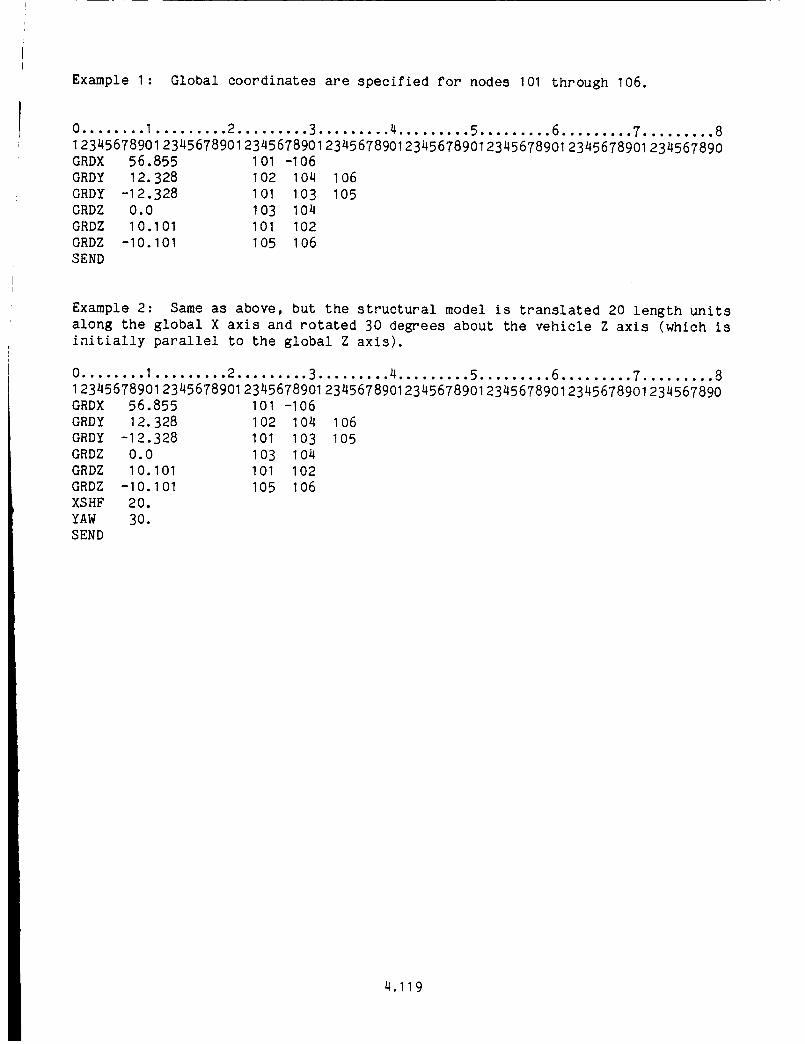
Example I: Global coordinates are specified for nodes 101 through 106.

0 ........ I ......... 2 ......... 3 ......... 4......... 5 ......... 6 ......... 7 ......... 8

12345678901 2345678901 2345678901 23456789012345678901 2345678901 2345678901 234567890GRDX 56.855 101 -106

GRDY 12.328 102 104

GRDY -12.328 101 103

GRDZ 0.0 103 104

GRDZ 10.101 101 102

GRDZ -10.101 105 106

SEND

I06

I05

Example 2: Same as above, but the structural model is translated 20 length units

along the global X axis and rotated 30 degrees about the vehicle Z axis (which is

initially parallel to the global Z axis).

0 ........ I ......... 2 ......... 3 ......... 4 ......... 5 ......... 6 ......... 7 ......... 8

123456789012345678901 2345678901 23456789012345678901 2345678901 2345678901 234567890GRDX 56.855

GRDY 12.328

GRDY -12.328

GRDZ O.0

GRDZ 10.101

GRDZ -10.101

XSHF 20.

YAW 30.

SEND

101 -106

102 104

101 103

103 104

101 102

105 106

I06

105

4.119

4.5 SINGLEANDMULTIPOINTCONSTRAINTS- GROUPE

Single and multipoint constraints are specified with three key words:

SPC - Single point constraints.

MPC - Multipoint constraints.

APPL - Applied generalized displacements.

ACEL - Applied generalized accelerations.

Each node can have up to 6 degrees of freedom, specified in the order u, v, w,9x, ey, ez

where

DOFI z u, translation in global x-directlonDOF2 _ v, translation in global y-directionDOF3 _ w, translation in global z-directionDOF4 -- ex, rotation about global x-axisDOF5 -- ey, rotation about global y-axisDOF6 0z, rotation about global z-axis

4.120

4.5.1 Single Point Constraints (SPC)

Input for the single point constraints appear on cards containing the key wordSPC, followed by the NBNDparameter in a slx-digit word describing the boundarycondition for each of the six DOFfor a node in the order of u,v,w,ex,ey,e z.

The NBNDparameter uses the following system:

0 - Denotes a completely fixed degree of freedom

I - Denotes a free degree of freedom

2 - Denotes that a prescribed value of displacement or acceleration is to be

specified for the degree of freedom

The nodes that are applicable to the specified boundary condition follow on the

input card, right justified in fields of five. All the shorthand notation described

in Section 3.1 can be used. That is, nodes I through 100 are written 1-100 and nodes

2, 4, 6 ... 100 are written 2-2-100. Any number of continuation cards may be used for

a given specification. However, the columns specifying the boundary conditions (i.e.,

columns 6 through 11 ) are ignored on the continuation card. A zero or blank field of

five (i.e., I5 field) terminates the card scan for a given boundary condition

specification. If the last field of a card (columns 76-80) is the last specification,an additional blank card (continuation card) must follow.

If a node's boundary conditions are not set on an SPC card, then all the degrees

of freedom are assumed to be free. In an idealization that contains beam or plate

elements this default is equivalent to 6 free degrees of freedom (NBND = 111111). It

should be noted in that case, that rotational degrees of freedom should be fixed for

all nodes that do not connect beam or plate elements; that is, nodes that have no

rotational stiffness or inertia assigned. To avoid the singular coefficient matrix

caused by the missing stiffness and inertia, DYCAST will detect a zero on a main

diagonal of the coefficient matrix, replace it with the value 1.0, and print a warning

message. If there are no externally applied moments for the rotational DOF, the

solution for rotation will still be zero, since there will be no internal (stiffness)

moment. Therefore, the rotational boundary conditions do not have to be fixed by the

user, but this fixity is recommended to reduce the total number of DOF required for

the solution.

If a problem has no beam or plate elements (no rotational degrees of freedom) the

_o._ _,, Is these•._er.a_y set 1! ..... Any ............... w._ can be

chansed by settln$ the appropriate default condition on the first SPC card with all

nodes used in the problem specified. The last specification for any node will be the

one used. There is no limit to the number of nodes in the SPC list, but a maximum of

200 different combinations of 0, I, and 2 can be used in the six digit NBND word.

4.121

4.5.2 Applied Displacements (APPL)

Applied displacements can be specified only for static solutions (STATin GroupA). If prescribed values are to be specified for any of the degrees of freedom, thevalue is input on additional cards, that appear after the SPC's and MPC's. Note thatthe complete applied displacement at any node is the product of the displacement

factor APPL for the node and the time function PTME of Group I.

The applied displacement cards (APPL) and multipoint constraint cards (MPC) can

be mixed in any order following the SPC cards, but they must be preceeded by a card

containing either of the key words APPL or MPC alone on the card. The following cards

contain the key word APPL, the node number, degree of freedom number, and the

prescribed value. The degree of freedom number is input as a number from I to 6

according to the component whose displacement is being specified, as in p. 4.120.

Example I: Beam clamped at both ends, uniform transverse load through shear center

(no torsion) along an axis of symmetry of cross section (planar deformation)

T y II

/,_ , J , I J i I i j I

A

, 2 3 4 s 6 7 8 9 _o I_

2 CLAMPEDBEAM 1

ct

x

0 ........ I ......... 2 ......... 3 ......... 4 ......... 5 ......... 6 ......... 7 ......... 8

1234567890123456789012345678901234567890123_56789_123456789012345678901234567890

SPC 000000 12 I

SPC 010000 11

SPC 110001 2 -10

NOTE: Node 12 defines the initlal orientation of the beam cross sectional axes and

since it is not part of the structural model it must be fixed. The SPC card for nodes

2-10 need not have been specified if three-dimensional beam elements are used but was

included as shown to reduce the number of DOF to the minimum.

4.122

Example 2: Rectangular membranepanel under doubly symmetric in-plane loads withunrestrained edges.

Y

_1 _3 _5

305

101 103 105

ICL RECTANGULAR MEMBRANEI

x q.

0 ........ I......... 2......... 3 ......... 4 ......... 5......... 6......... 7 ......... 8

123456789_123456789_123456789_123456789_123456789_123456789_123456789_123456789_

SPC 000 101

SPC 100 103 105

SPC 010 301 501

SPC 110 303 305 503 505

NOTE: The default conditions for membrane elements alone is 111000, and the

rotational DOF need not be specified in this problem, since no beam or plate elements

exist.

Example 3: Same as Example 2 with displacement factor of 0.04 applied in the y-

direction at nodes 501, 503, 505.

0 ........ I......... 2 ......... 3......... 4......... 5 ......... 6 ......... 7 ......... 8

12345678901234567890123456789012345678901234567890123456789012345678901234567890

SPC 000

SPC 100

SPC 010

SPC 020

SPC 110

SPC 120

APPL

APPL 501

APPL 503

APPL 505

101

103 105

301

501

303 305

5O3 5O5

2 0.04

2 0.04

2 0.04

NOTE: The first APPL card must be without data, if it is the first card following

the SPC set.

4.123

4.5.3 Multipoint Constraints (MPC)

The program implements a multipolnt constraint capability of the formn

6di = _ aij_j (4.5.1)j=1

where _i is the ith dependent degree of freedom, aij are prescribed coefficients and

6j are a set of independent degrees of freedom.

These constraints are specified on input cards that appear after the SPC input.

The applied displacement cards (APPL) and multipoint constraint cards (MPC) can be

mixed in any order following the SPC cards, but they must be preceded by a delimiter

card containing either of the key words APPL or MPC alone on the card.

This delimiter card is followed by cards containing the dependent node number and

degree of freedom (left hand side of Eq. 4.5.1) along with the independent node

number, degree of freedom, and a_ (right hand side of Eq. 4.5.1). Each card canzj

accommodate up to two independents of the equation. Any number of continuation cards

can be used and are indicated by leaving the dependent node specification blank on

succeeding cards.

When a degree of freedom (DOF) is dependent it must also be deleted (set to zero

as if fixed) on an SPC input card and it may not appear as an independent in any

constraint equations, because it is eliminated from the set of unknown DOF.

If a node has been assigned any added inertia in Group G, each of its DOF can

have at most only one term in its dependency equations, i.e., can be dependent on onlyone other DOF.

A current restriction exists in the program that allows applied displacements and

dependent degrees of freedom to be written at a maximum of 200 nodes and with a

maximum of 500 coefficients aij in total.

4.124

Example I :

The displacement u at node 100 is related to independent degrees of freedomaccording to the following equation:

u100 = 0.5 u10 + 0.5 u11 + 0.25 u12

0........ I ......... 2 ......... 3 ......... 4 ......... 5......... 6 ......... 7......... 812345678901234567890123456789012345678901234567890123456789012345678901234567890MPCMPC 100 I 10 I 0.5 11 I 0.5MPC 12 I 0.25

NOTE: The first MPCcard, without data, is only necessary if this is the first cardfollowing the SPCset.

Example 2: Rectangular panel, fixed on one edge, uniform shear displacement on theopposite edge.

Z

0.059 4

IIIIIIIII 2

Nodes I and 2 are fixed. There is an applied displacement at node 3 in the negative y

direction. The distance between nodes 3 and 4 remains constant. Line 3-4 remains

parallel to line I-2

0 ........ I......... 2 ......... 3......... 4......... 5 ......... 6 ......... 7 ......... 8

12345678901234567890123456789012345678901234567890123456789012345678901234567890

SPC

SPC

APPL

APPL

MPC

MPC

000 I 2 4

021 3

3 2 -0.050

4 2 3 2 1.0

4 3 3 3 1.0

NOTE: The SPC cards must specify zero for node 4 degrees of freedom 2 and 3 because

they are effectively eliminated from the solution (they are dependent degrees of

freedom). (An alternative procedure can be to specify the same SPC and APPL for node

4 as for node 3, and delete the dependencies. This is a slightly different condition,

in that edge 3-4 is then allowed to rotate.)

4.125

4.5.4 Non-Global Constraints (MPC)

The multipoint constraints can be used to transform displacements at a node toanother coordinate system. Thus, the MPC'scan be written as

_i= el _i + _2 _j + _3 _'k

6j = BI _i + B2 _j + B3 _k

_k = YI _i + Y2 _j + Y3 _k

(4.5.2)

where the e, B, Y's are the direction cosines of rotation, _i' _j' _k are thedisplacements with respect to the original global directions, and _., _., _, arezthe components of displacements at the node with respect to the new coordinate system.

The new coordinate DOFwill replace the original global cartesian DOF, with the

appropriate transformations of the local stiffness, mass, loads, etc. Thus, the SPC

input must refer to the new coordinate DOF. This feature can be used if a node is

constrained in a non-global direction. It will be particularly useful for struc-

tures that conform to cylindrical or spherical coordinate systems. The output dis-

placements, velocities, and accelerations are transformed back to the global system.

The input for this feature is the same as for the standard MPC case with the

exception that the SPC's are not fixed to account for this type of MPC. However, they

may be fixed to account for constraints in the new coordinates.

Exampl e:

Y

For this problem the displacement u is set equal to zero and v (along Y) is

free. Assume there are no rotations or z displacements. The global coordinates of

the problem are x, y. Thus

u25 : u25 cos ¢ - v25 sin ¢ = -v25 sin ¢

v25 = u25 sin ¢ + 725 cos ¢ = v25 cos ¢

4.126

0........ I ......... 2......... 3......... 4......... 5......... 6....... ..7 ......... 812345678901234567890123456789012345678901234567890123456789012345678901234567890SPC 010000 25MPCMPC 25 I 25 I O.8660254 25 2 -0.5MPC 25 2 25 I 0.5 25 2 0.8660254

NOTE: On the SPCcard, node 25 degree of freedom I is specified to be 0 but node 25degree of freedom 2 is specified I or free since it remains an independent degree offreedom (although rotated). If the normal displacement _ were not fixed it would havea I boundary condition specified.

For this particular example, the terms involving _25 could have been omitted, sinceits value is set to zero by the SPC.

4.127

4.6 APPLIEDLOADING- GROUPI

The applied load is separated into the product of a spatial distribution functionand a time function

P(x, y, z, t) -- P1(x, y, z) F(t) (4.6.1)

The spatial distribution can be specified as concentrated loads at nodes in theglobal cartesian coordinate system or as a distributed loading on an element, whichloading is consistently assigned to the element node points.

The time function F(t) can be specified in three different ways as explainedlater. A simple single-phase (one time function for all load components) or morecomplex multi-phase (each componenthaving its own time function) loading can be used.

At each time step, the consistent nodal load components from the element-orlentedloads (BMLOand SURF)are calculated, transformed into globally-oriented components,and added to the globally-oriented concentrated loads (CONC). Each global loadcomponentat each node is then multiplied by the current value of the time functionassigned to it.

4.128

4.6.1 Concentrated Loads (CONC)

Concentrated loads are applied at nodes in the global coordinate system, and keeptheir orientation while following the node through its motions. These loads are inputas Group I data in a sequence of two input cards. The key word specification is

CONC. The first card in the sequence contains the key word, CONC, the node number

and the forces in the global x, y, z directions. The second card contains the key word

and the three moments with respect to the global x, y, z directions.

A CONC input card can be specified for any node point in the finite element

model. Example input are shown below:

Example I: Load factor 100 Newtons in the positive global x direction and moment

factor 55 Newton meters in the global y direction at node 105.

0 ........ I ......... 2 ......... 3 ......... 4 ......... 5 ......... 6 ......... 7 ......... 8

12345678 9012345678 9012345678 9012345678 9012345678 90123456789012345678901234567890

CONC 105 I00.0 O. 0 O. 0

CONC 0.0 55.0 0.0

Example 2: Applied load factors 25, 33, 15 lb at node 15 in positive x, y, z globaldirections, no moments

0 ........ I ......... 2 ......... 3......... 4 ......... 5 ......... 6 ......... 7 ......... 8

12345678 9012345678 9012345678 9012345678 9012345678 9012345678 9012345678 9012345678 90

CONC 15 25.0 33.0 15.0

CONC O. 0 O. 0 O. 0

4. 129

4.6.2 Line Load on a BeamElement (BMLO)

Line loads are specified in the element local coordinate system, and follow theelement orientation. The consistent load vector for a distributed line load on a beamelement is obtained from

I qi{f} _ f [N]t[Q]dx

o qj

(4.6.2)

where [N] is the shape function for the lateral displacement, [Q] is the distributionof the load from node i to node j. In DYCASTthe distributed line load can varylinearly betweeneach node. The quantities qi and qj are the magnitude of the loadingat each node in the local y and z directions. These quantities represent input and arein units of force per length or momentper length. The local y direction is towardsthe third node point thatspecifles the beamcoordinate system on the connectivityinput (Section 4.3.3) and local z is perpendicular to this direction. Thus theconsistent load vector f is defined in the local x-y and x-z planes. Thisspecification defines a following load which is always perpendicular to the currentbeamconfiguration.

Exm_ple I: Uniform load factor of 100 ib/in in the local y direction for elements I,2and3

0........ I ......... 2......... 3......... 4......... 5 ......... 6......... 7 ......... 8123456789_123456789_123456789_123456789_123456789_123456789_123456789_123456789_BMLO 100.0 100.0 0.0 0.0

I 2 3

The applicable membersare specified using usual notation as described in Section 3.

4.130

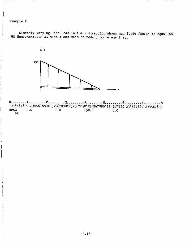
Example 2:

Linearly varying line load in the z-direction whose magnitude factor is equal to150 Newtons/meter at node i and zero at node j for element 95.

I z

15o _

• I_ X

0 ........ 1 ......... 2 ......... 3 ......... 4 ......... 5 ......... 6 ......... 7 ......... 8

12345678901234567890123456789012345678901234567890123456789012345678901234567890

BMLO 0.0 0.0 150.0 0.0

95

4.131

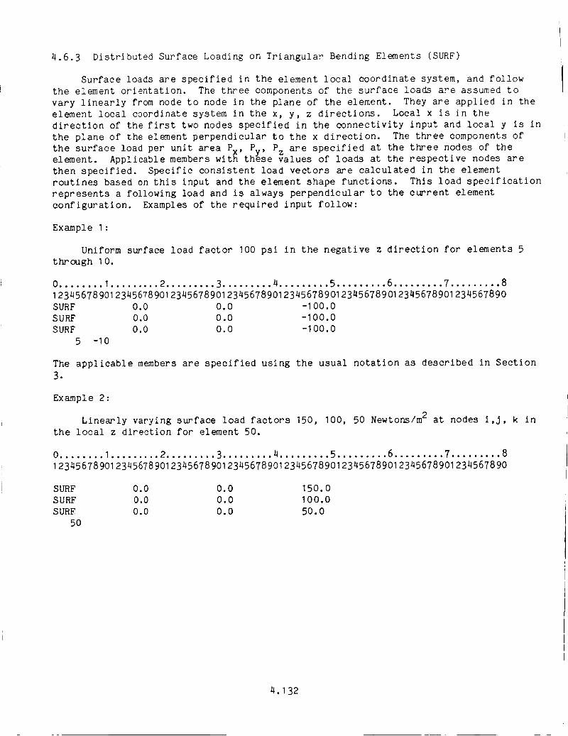
4.6.3 Distributed Surface Loading on Triangular Bending Elements (SURF)

Surface loads are specified in the element local coordinate system, and followthe element orientation. The three componentsof the surface loads are assumedtovary linearly from node to node in the plane of the element. They are applied in theelement local coordinate system in the x, y, z directions. Local x is in thedirection of the first two nodes specified in the connectivity input and local y is inthe plane of the element perpendicular to the x direction. The three componentsofthe surface load per unit area Px' P ' P- are specified at the three nodes of they _element. Applicable members with these values of loads at the respective nodes are

then specified. Specific consistent load vectors are calculated in the element

routines based on this input and the element shape functions. This load specification

represents a following load and is always perpendicular to the current element

configuration. Examples of the required input follow:

Example I :

Uniform surface load factor 100 psi in the negative z direction for elements 5

through I0.

0 ........ I......... 2 ......... 3 ......... 4......... 5 ......... 6 ......... 7 ......... 8

12345678901234567890123456789012345678901234567890123456789012345678901234567890

SURF 0.0 0.0 -I00.0

SURF 0.0 0.0 -100.0

SURF 0.0 0.0 -100.0

5 -I0

The applicable members are specified using the usual notation as described in Section

3.

Example 2 :

Linearly varying surface load factors 150, 100, 50 Newtons/m 2 at nodes i,j, k in

the local z direction for element 50.

0 ........ I......... 2 ......... 3 ......... 4 ......... 5 ......... 6 ......... 7 ......... 8

12345678901234567890123456789012345678901234567890123456789012345678901234567890

SURF 0.0 0.0 150.0

SURF 0.0 0.0 100.0

SURF 0.0 0.0 50.0

50

4.132

4.6.4 Load Factor Time Functions (PTME,PTM2,PTM3)

The time variation functions for the applied loads are specified in tabular formof load factor versus time. Values of the load factor, PI' and load factor increment,API , are obtained by interpolation within these tables. If the maximumtime in atable is exceeded, the load factor is held constant at the last value, with zeroslope. Up to 50 points can be input per table. The tables must be in order ofincreasing time, starting from t _ O.

This input is required whenever a spatial distribution of applied load (CONC,BMLO,or SURF)or displacement APPLis specified. If it is not input an error messageis printed and the job is aborted.

There are three types of time functions available. The first (PTME)involvesonly one commontime function for all the applied loads (single-phase loads). Thesecond (PTM2)allows different time functions to be specified at different nodes, butall the six componentsat any node will have one time function. The third (PTM3)allows a different time function for every load component. Oneof these three timefunctions must be used whenever applied loads are specified.

The applicability of the various time functions is given in the following table:

Applied ApplledTime Applied loads Displacement AccelerationFunction CONC BLMO SURF APPL ACEL

PTME Yes Yes Yes Yes No

PTM2 Yes Yes Yes No No

PTM3 Yes Limited* Limited* No No

ACELT No No No No Yes

*Small rotations

These time functions are all applied to the globally-oriented nodal components.The BMLOand SURFare element-oriented loads that follow the elements as they move,and lead to globally-oriented nodal force componentswhosemagnitudes will vary withthe rotation of the elements. Thus, the time functions are applied to the resultingglobal load components, not to the element-oriented load components. There will be nodifference in the results except for the cases where different PTM3time functions areassigned to more than one force component or more than one momentcomponentat thesame node for the element-oriented BMLOand SURFload inputs. In these cases, theloads applied to the nodes can not generally be predicted in advance, and will not bethose desired, except when the element rotations are small. Therefore, the use ofPTM3with BMLOor SURFis limited to small rotations in these cases. As a result, thePTM3is not generally recommendedfor use with the BMLOor SURFloads.

In cases where most of the load componentsshare the same time function, and asmall number of componentshave different time functions, it will be useful to use thePTMEinput for the most commontime function and then use either the PTM2or PTM3timefunctions for the exceptions.

4.133

If the time step used in the solution of a problem is comparable to or large thanthe period of an oscillating load function, or comparable to or larger then the timeinterval betweenabrupt changes in a nonlinear load function, then someportion of theinput load function will be ignored. This is similar to the errors incurred in usingtoo large a digital sampling rate for rapidly varying data. Therefore, if all thedetails of the input load function are important, than the user should insure that thetime steps are small enough to follow the input function with sufficient accuracy.This can be done by using a maximumtime step (DTMAX)on the NEWM,STAT, or WLSNcards. However, small time steps can be costly, so the input load function should useas large a time interval or be as smooth as possible, to avoid unnecessary reductionsin the solution time step.

The load factor versus time tables must also be input for a static analysis inorder to define the load factors and load increments Here the time is used as aparameter defining these quantities. If a table contains one straight line segment(constant rate) then the load factors are proportional to time, and the load rate is aconstant. A variable load step procedure in a static analysis can be defined byinputting a numberof linear segments. This will be demonstrated in the followingexample.

Example:

Variable load step static analysis (i.e., decreasing slope)

0........ I ......... 2......... 3.. ....... 4......... 5 ......... 6......... 7......... 812345678901234567890123456789012345678901234567890123456789012345678901234567890PTME 0.0 0.0PTME I. 0 I .0PTME I. 5 2.0PTME I. 75 3.0

Note that the time step is used to obtain the load and the load step frcm the table.Assuming that the time step will be constant, the load steps may not be constant. Ifsufficient nonlinearities are involved, then the convergence criteria may force thetime step and therefore the load step to vary further throughout the problem.

For the special case of applied displacements, the global spatial displacementdistribution (APPL) is multiplied only by the common time function (PTME), and is thus

restricted to single-phase behavior. The APPL input is described earlier in Group E,

p. 3.47.

The applied acceleration time function ACELT is used only for the applied

accelerations ACEL, but is included in the above table of time functions for

completeness. It is discussed in the next section.

4.134

4.6.5 Gravity Load or Weight (GRAV)

The main purpose of imposing gravity has been to compute the gross (rigid body)motions of a vehicle as it interacts with and rebounds from an impact surface. It isnot intended here to compute accurately the stresses and deformations due to gravity,although that mayresult in somecases.

Distributed gravity forces (weights) can be imposed at the nodes parallel to anyone of the global axes, using the GRAVinput in Group I. These nodal weight vectorsare added to the set of external load vectors (P in Eq 1.3.9 on p. 1.13), with thefollowing condi tions:

o Each element's weight is distributed amongits nodes in such a way that theresultant gravity force acts at its center of mass. The offset beamelement isan exception as discussed below.

o The weight of any user-specified lumpedmass is also added to each node.o The resulting total weight at each node is equivalent to the total mass at the

node multiplied by g, the acceleration due to gravity.o The time variation for dynamic problems is a step function starting at t=O and

constant for all subsequent time.

In lumping the weight vectors at the nodes, two simplifications have been made.First, the bending momentsat the nodes of BEAMand TRP2elements, caused by gravityacting on the distributed mass of an element, have been neglected. This means thatthe bending within an element induced directly by the weight is ignored, but thebending developed in the structure due to the weights placed at the nodes isincluded. Thus a model composedof only one beamor plate element will not deformcorrectly under gravity, because all the weights are placed at the nodes which are onthe boundary. The finer the model the moreaccurate the gravity solutions become.This limitation should lead to negligible errors in typical vehicle models where thesize of individual elements are small comparedto the total size of the model.

Second, the beamelements have their weight placed at their end nodes, and not ontheir centroidal axes. In actuality, a beamthat has its end nodes offset from thelongitudinal centroidal axis will develop a torque about the nodal axis due to thegravity forces. This gravity torque is neglected in the beamelement, but might besignificant when the gravity forces and accelerations (Ig) are dominant or are asignificant part of the total forces and accelerations in the problem, and the beamelements have large offsets between their nodal and centroidal axes. Therefore, theproblem solution could be significantly in error when gravity is the only load andlarge beamoffsets are present. However, in the majority of vehicle crasho,mu_a_ns, the gravity loads and Ig _,_-ation are sma_ compared to ......by the impact, and this error will have a negligible effect on the structuralresponse. Note that this error does not diminish as the model is refined by merelyincreasing the number of beamelements. However, an accurate portrayal of thisgravity torque can be madeby linking the offset nodes to a set of nodes on the beam'scentroidal axis, using short "rigid" beams.

4._35

It should be noted that, in dynamic problems, the step function time variation of

the gravity loads is well-sulted for initial conditions in which a vehicle is in a

free-fall condition prior to impact. That is; there are no other external loads

besides the weight, and the vehicle is then accelerating at Ig. In this case, there

will be no initial structural deformations due to gravity, since each node is

accelerated at exactly Ig. However, when any part of the weight is reacted by an

external force, such as a ground reaction or aerodynamic lift, the program will solve

the dynamic response of the structure to the distributed gravity forces applied as

step functions in time. To-avoid this transient response, the nodes must be given an

initial displacement which places the entire structure in static equilibrium with the

applied loads. These static displacements are obtainable a from one-step static

solution of the gravity load problem, and can then be introduced as inital

displacements (IDSP) input in the dynamic problem.

4.136

4.6.6 Applied Acceleration (ACEL, ACELT)

Acceleration versus time functions can be specified for any motion componentatany node, using the ACELand ACELTinputs. The resulting velocities and displacementsare calculated using the acceleration versus time function and the initial values ofvelocity and displacement specifed in the ACELTinput card set. Since the appliedacceleration leads to an applied displacement, which is a type of constraint, the ACELcard is used in Group E input - Constraints. Also in Group E, the constraint codeNBND_ 2 must be specified for the appropriate node and DOFon an SPCcard, as in thecase of applied displacement.

The variation of the acceleration function within the time step is ignored whencalculating the accelerations; only the input acceleration value at the end of a timestep is used directly. However, the numerical integrations to calculate the resultingvelocity and displacement use the entire input acceleration function within a timestep. Therefore, in a linear problem (small deformation elastic) there will be nosignificant loss of accuracy in using the input acceleration versus time function dueto large time steps, since the applied accelerations and the resulting velocities anddisplacements will be correct at the end of each step. A nonlinear problem, on theother hand, is path dependent because conditions of plasticity, failure, and largedeformations may occur within a large time step interval that will change thesubsequent behavior and therefore these intermediate states cannot always beignored. If the input acceleration function is changing rapidly, the time step usedin the solution must be small enough to sample accurately this varying function. Thisis particularly important if there are peak acceleration amplitudes within a timestep. The time step can be limited by use of the maximumtime step input (DTMAX)onthe NEWM,STAT, and WLSNinput cards. However, small time steps can be costly, so thetime intervals used in the input acceleration functions should be as large aspossible, and the acceleration functions as smooth as possible, to avoid unnecessaryreductions in the solution time step.

4.137

This page intentionally blank

4.1 38

5.0 DATA PREPARATION FOR PREPROCESSING AND POSTPROCESSING

This section describes the input for the SATELLITE and GRAFIX programs used for

pre- and postprocessing of input and output.

SATELLITE has the capability of reading and checking input data and plotting the

undeformed and deformed structural idealization. Additionally, an option exists to

calculate the ordering of the external node numbers that lead to the minimum

semibandwidth.

GRAFIX was written to postprocess data from a DYCAST restart file. The program

currently reads data from a restart file and produces plots of the histories of

displacement, velocity, and acceleration.

5.1

5. I INPUTPREPARATIONFORSATELLITE

The input data cards must be in the sequence given here.

/ Card : Key Word DYCA Columns I-4/

This required card uses four-character words as follows:

DYCA The SATELLITE program can be used with a number of nonlinear programs. The keyword for DYCAST is DYCA in the first four columns.

A number of options are available. These are specified by additional words on

Card I in fields of four. These can be consecutive on the card or any multiple of

four spaces can be skipped on the input card, between these key words. The available

options and key words are:

BAND Specifies that the optimum nodal sequence that minimizes the semibandwidth is

to be determined. In this case the optimum order of the external node numbers

for DYCAST Group B input data will be printed and output to a card image

file. The original Group B nodal list should be replaced by this optimized

Group B list. If this key word is not specified the bandwidth will not be

optimized.

NOTE: Connectivities provided by multipoint constraints (MPC) will be ignored

here! Thus two substructures connected only by MPC will be seen as two

separate bodies, and only one will be optimized. This can be corrected by

temporarily connecting the MPC'd nodes by dummy stringer elements for

bandwidth optimization only.

SCAN Process and check input data but do not produce any plots.

PRIN Print transformed coordinates to be plotted.

REST Read an existing DYCAST restart file and produce deformed plots.

SATELLITE can be used as a preprocessor to check input by plotting the undeformed

finite element model or it can be used as a postprocessor to plot the deformed finiteelement model.

Format Columns S_mbol Comments

A4 I-4 DYCA key word for DYCAST processing.

19A4 5-80 Any of the optional words listed above.

Multiples of four blank columns can be

inserted between key words for spacing

appearance.

5.2

/ Model Data/

Preprocessing - Plot Undeformed Finite Element Model

The DYCAST input data deck (defining the finite element model) starting with the

title card, follows the DYCA Card when producing undeformed plots. The minimum

required input is from the title card through the nodal coordinates Group D, followed

by a STOP or END card. Additional parts of the input deck beyond Group D will be

ignored until a STOP or END card is reached. Alternatively, the entire deck may be

input, starting from the title card. The title in the DYCAST deck will be used on the

plots.

Postprocessing - Plot Deformed Finite Element Model

When deformed views are desired, specify the REST word on DYCA card above. This

indicates that input will be from a restart file previously generated by DYCAST.

Consequently, the input data deck should not be included. All that is necessary here

is a title card that is used to label the plots produced by SATELLITE.

The file identification and loading instructions are part of the system JCL or

procedural commands that preceed the DYCAST input.

5.B

/ Plot Types/

This required card determines the type of plots desired. Five different types

of labeled pictures can be obtained. These are specified with the fixed point

numbers right justified in any of the fields of five as follows:

2 --

3--

4 --

5 --

Format

Numbered unconnected nodes

Numbered nodes, unnumbered members

Numbered nodes and members

Unnumbered nodes, numbered members

Unnumbered nodes and members

Columns Symbol

I5 1-25

Comments

As many of the number codes above as desired,

in every fifth column

NOTES:

I.

o

A complete set of plots is repeated for each of the types requested here.

Thus, if 10 plots are requested by the following set of cards, and codes 3 and

5 are specified here, then 20 plots will be made, 10 for code 3 (numbered

plots) and 10 for code 5 (unnumbered plots).

Plotting parameters can appear in groups, starting with a "plot type" card and

ending with a REPT card. Several such groups can be used, one after the

other, in the same input.

5.4

/ Initial Plane/

This required card defines the initial viewing plane as one of the model's three

global coordinate planes, and orients it either horizontally or vertically on the

image plane. Three characters are specified, corresponding to any sequence of the

model global axes, x, y, z. The first designates the model global axis to be in the

positive longitudinal (usually rightward horizontal) direction in the image surface;

the second in the positive transverse direction (usually upward vertical); and third

in the positive normal direction (toward the viewer). For example, yzx defines a view

of the global yz plane with y to the right, z upward, and x toward the viewer.

The angles ALPHA, BETA, GAMMA on the next card set called "Viewing Angle and Time

Increments" are applied to this initial coordinate view to produce the first view to

be plotted.

Format Columns

3AI I-3

3AI 4-6

S_mbol Comments

Any permutation of xyz

Input the three characters +++ here

(required)

NOTES :

I. The characters +++ in columns 4-6 are required, but are currently inactive.

5.5

/ Viewing Angle and Time Increments/

This required set of one or two cards alters the initial viewing angles and

increments the angles for a sequence of rotated plots. These cards also contain

controls on the time steps to be used in plotting a deformed structure from a DYCAST

restart tape.

ALPHA, BETA, and GAMMA are initial angles added to the coordinate view specified

in the "Initial Plane" card that preceeds this set.. ALPHA is the rotation applied

about the positive longitudinal axis (usually rightward horizontal) in the image

surface, BETA about the positive transverse (usually upward vertical) axis, and GAMMA

about the outward axis toward the viewer. They are applied in the sequence given, and

follow the right- hand rule for positive rotations. Thus a positive ALPHA rotates the

top of the image towards the viewer. Zero values for all three angles will leave the

orientation as specified on the "Initial Plane" card.

The first plot will have the orientation determined by the "Initial Plane" card

plus the initial angles ALPHA, BETA, GAMMA. The image will then be rotated by addingone increment each of INCA, INCB, INCG in sequence, and then the next plot will be

made. Another set of angle increments will be added, and the next plot made, and so

on.

(continued on next page)

5.6

/ Viewin_ An_le and Time Increments/ continued from previous page

Card I :

Format Columns Symbol Comments

I5 1-5 INCA Increment of ALPHA (degrees).

EIO.O 6-15 ALPHA First value of rotation angle about the

longitudinal axis in the image surface

(degrees).

15 16-20 INCB Increment of BETA (degrees).

El O. 0 21-30 BETA First value of rotation angle about the

transverse axis in the image surface (degrees).

I5 31 -35 INCG Increment of GAMMA (degrees).

El O. 0 36-45 GA_@4A First value of rotation angle about the normal

axis, out of the image surface (degrees).

I5 46-50 MAXROT Total number of rotational increments to be

plotted in a series, including the first

(Default = I for only one view).

El O. 0 51 -60 X Max. dimension of plot in the transverse or

vertical direction in the image surface.

Depends on the plotting device used.

(the following fields are only for deformed plots from a restart tape)

I5 61 -65 IFACT Scale factor to magnify deformations

(default = I).

I5 66 -70 LST Time step number for first plot, from

DYCAST run that generated restart file.

Use only for automatic time step incrementing.

I5 71 -75 INC Increment of time step number. Use only for

automatic incrementing.

I5 76-80 NTLPM Final time step number from DYCAST run. Use

only for automatic time step incrementing.

(continued on next page)

5.7

/ Viewing Angle and Time Increments/ continued from previous page

Deformed plots can be requested at individual time steps. This is done with the

following optional card input. This input is initiated by setting LST, INC, and NTLPM

equal to zero or blank (blank field columns 66-80) on Card I above.

Card(s) 2: optional

Format Columns

1615 1-80

Symbol Comments

Specified individual time steps for which the

model is to be plotted from generating run of

DYCAST (see Sect. 4.1.4), in increasing

numerical order. Up to 50 can be specified.

As many cards as needed can be used. A blank

I5 field ends the data list. If list ends in

last I5 field on a card, a blank card must

follow.

NOTES:

]. The DYCAST output file will not contain data for every time step if KPRINT>I

was used on the REST card (p. 3.17) in the DYCAST analysis. In that case, the

deformed model cannot be plotted at the "lost" time steps.

5.8

/ Deletions/

This required card allows the user to delete entire element types from the plot.

BEAM

TRIM

STRG

SP NG

TRP2

GRDS

will omit all beam elements

will omit all triangle membrane elements

will omit all stringer elements

will omit all spring elements

will omit all triangular plate elements

will omit all contact elements

If there are no element types to be omitted, a blank card must be specified. For

example, to plot only BEAM elements, specify TRIM, STRG, SPNG, and TRP2 on this card.

Format Columns Symbol Comments

4(A4,1X) 1-20 Any of the four character words

listed above, with one blank space betweenthem

21 -80 Blank

NOTES :

I •

2.

A blank card must be used if all types of elements are to be plotted.

To de].ete all elements, plotting only nodes, input the number I on the "Plot

Type" card discussed above.

5.9

/ Nodes/

This required set of at least two cards specifies nodes tobe included in

scaling the plot. The plot will be scaled to get all nodes specified here

onto the image surface. Therefore, the nodes specified here should at least

include all the nodes attached to elements to be plotted. However, the size

of the plot can be reduced by including additional nodes that are not attached

to elements to be plotted. This is a useful method for controlling the size

of partial views of the model. For example, if the part is be to drawn to the

same scale as the total structure all the nodes in the structure should be

input. If a part of the structure is to be plotted to the maximum size, these

cards should include only the nodes that are in that part.

A blank card or card with only zero entries ends this card set.

Card(s) I :

Format Columns Symbol Comments

16 I5 I-80 NODE Node list as described above. All the

shorthand notations are allowed. Any number of

continuation cards are allowed.

Card 2:

A blank card is required here.

NOTES :

I , If all nodes are to be included, it is sufficient to specify only one negative

number whose absolute magnitude is greater than the largest node number in the

model.

o An inclusive range of numbers can also be specified even though not all the

numbers within the range are used for nodes. In this input, node numbers

specified but not used in the model are ignored, as a convenience. For

example, this input can specify nodes 1000-1999, although 1200-1299 do not

exist in the model.

5.10

/ Elements/

This required set of at least two cards specifies elements to be included in

the plot. Input format is the same as for "Nodes" above. All nodes associated with

the element to be plotted must be specified on "Nodes" card set. A blank card or card

with only zero entries ends this card set.

Card(s) I :

Format

1615

Columns Symbol

I-80

Comments

Member numbers as described above. All

shorthand notations and any number of

continuation cards are allowed.

Card 2:

A blank card is required here.

NOTES :

I.

,

If all the elements are to be plotted it is sufficient to specify one negative

number in the first I5 field whose magnitude is greater than the largestelement number in the finite element model.

An inclusive range of numbers can also be specified even though not all

numbers within the range are used. For example, specification can be made for

elements 1000-1999, although 1200-1299 do not exist for that job.

5.11

/ End of Data/

This required card contains one of the control words STOP or REPT in columns

I-4 to end the job or to redefine a different set of plotting parameters, as

follows:

Undeformed Plots - preprocessing from a DYCAST input deck.

If the control word is:

STOP, and a STOP card ended the DYCAST input deck, this is the last card

of the SATELLITE input•

STOP, and the DYCAST input deck ended with an END card, to indicate that

another DYCAST input deck follows, then the next input deck will be

processed, subject to the same SATELLITE plotting commands.

REPT, then another set of SATELLITE input cards will follow, starting

with a "plot type" card (p.5.4), to define new plotting parameters for

the same model.

Deformed Plots - post processing from an existing DYCAST restart file. If the

control word is:

o STOP, this is the last SATELLITE input card.

o REPT, then another set of SATELLITE input cards will follow, starting

with a "plot type" card (p. 5.4), to define new plotting parameters for

the same analysis results.

Format Columns Symbol Comments

A4 I-4 Either STOP, or REPT, as discussed above.

NOTES :

I • A special default case is available, for which the input consists only of the

initial DYCA card, the model data file, and a STOP card. In that case, only

one plot will be produced, of the undeformed model, viewing the XY plane along

the Z axis, with all nodes and elements included and unnumbered. Either the

DYCAST input deck or the DYCAST restart file can be used for the data fileo

5.12

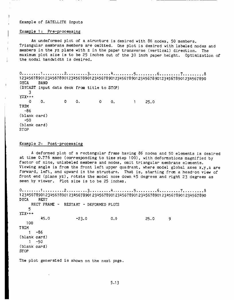
Example of SATELLITEInputs

Example I : Pre-processin_

An undeformed plot of a structure is desired with 86 nodes, 50 members.

Triangular membrane members are omitted. One plot is desired with labeled nodes and

members in the yz plane with z in the paper transverse (vertical) direction. The

maximum plot size is to be 25 inches out of the 30 inch paper height. Optimization ofthe nodal bandwidth is desired.

0 ........ I ......... 2 ......... 3 ......... 4 ......... 5 ......... 6 ......... 7......... 8

123456789_123456789_123456789_123456789_123456789_123456789_123456789_123456789_DYCA BAND

(DYCAST input data deck from title to STOP)

3YZX+++

0 O.

TRIM

-86(blank card)

-50

(blank card)

STOP

0 O. 0 O. I 25.0

Example 2 : Post-processin_

A deformed plot of a rectangular frame having 86 nodes and 50 elements is desired

at time 0.776 msec (corresponding to time step 100), with deformations magnified by

factor of nine, unlabeled members and nodes, omit triangular membrane elements.

Viewing angle is from the front left upper quadrant, where model global axes x,y,z are

forward, left, and upward in the structure. That is, starting from a head-on view of

front end (plane yz), rotate the model nose down 45 degrees and right 23 degrees as

seen by viewer. Plot size is to be 25 inches.

0 ........ I ......... 2 ......... 3 ......... 4 ......... 5 ......... 6 ......... 7 ......... 8

123456789012345678901 2345678901 2345678901 2345678901 2345678901 2345678901 234567890DYCA REST

RECT FRAME - RESTART - DEFORMED PLOTS

5YZX+++

45.0 -23.0 0.0 25.0 9

100

TRIM

I -86

(blank card)

I -50

(blank card)

STOP

The plot generated is shown on the next page.

5.13

ALPHA = 45. BETA = --23. GAMMA = 0.

Y Z X ÷ + +

RECT FRAME - RESTART- DEFORMED PLOTS

SCALE FACTOR 9_ 'INCREMENT NO. 100 TIME 0_00775987

0199-012(T)

5.14

5.2 INPUTPREPARATIONFORGRAFIX

The GRAFIXpost-processing program can read a DYCASTrestart file and printplot displacement, velocity, and acceleration versus time for any degree-of-freedom. The input is as follows:

and

/ Any 80 Character Title/

This required title card serves as a heading for all pages of output and for all

plots.

5.15

/ Key Word PRIN/

This optional set of cards is used when a printout is desired of displacement,

velocity, and acceleration for each node at specified time increments from a DYCASTrestart file.

NOTES :

I.

2.

Format Columns Symbol

A4 I-4 PRIN

1415 11-80 INC

Comments

Print data.

Time step numbers from DYCAST run,

corresponding to the times at which data are

to be printed. Each time has an associated

unique increment number. If data are not

printed in the original generating run, it

can be retrieved and printed with this

option. The short form input described in

Section 3.1 may be used. That is, I through

100 is written as I - 100 and 2, 4, 6 ...

100 is written as 2-2-100. Any number of

continuation cards can be used of the same

format as the first card. If the short form

notation is used, its specification must be

complete on one card.

Either the PRIN or the PLOT set or both may be used.

The DYCAST output file will not contain data for every time step if KPRINT>I

was used on the REST card (p. 3.17) in the DYCAST analysis. In that case, the

data cannot be printed for the "lost" time steps.

5.16

/ Key Word PLOT/

This card begins the parameters for a group of plots of data versus time.

Format Columns S_mbol

A4 I-4 PLOT

5-10

I5 11-15 INCI

I5 16-20 INC2

I5 21 -25 GSCL

Comments

Plot specified data

Blank

Initial increment number to be plotted

Final increment number to be plotted

Acceleration is always plotted in g's.

(Ig = standard gravitational acceleration

at earth surface).

If GSCL = I or blank; units of the DYCAST

run to be plotted are inmeters per sec _,

g = 9.800m/sec 2

= 2; units are in inches persec ; g = 386.088in/sec 2

= 3; units are in feet per sec2;

g = 32.1740ft/sec 2

NOTES :

I.

.

o

If this PLOT option is specified the following cards determine the variables

to be plotted and necessary scale factors. Many of these cards have default

values that allow the card to be omitted.

Plotting parameters appear in groups starting with a PLOT card and ending with

a SEND card. Within a group, the XLEN, XSCALE, YSCALE, and Plot Type card

sets define the parameters for a group of plots. These card sets can appear

in any order within the group. As many groups as desired may be used, one

after the other, in an input deck.

The DYCAST output file will not contain data for every time step if KPRINT>I

was used on the REST card (p. 3.17) in the DYCAST analysis. In that case, the

data cannot be plotted for the "lost" time step.

5.17

/ Key Word XLEN/

This optional card specifies the physical dimension of the time scale for all the

plots in a group (between PLOT and SEND cards).

Format Columns Symbol Comments

A4 J -4 XLEN

5-I0

I5 11-I5 LENGTH

16 -80

Blank

Length of abscissa in inches, with

scale markings every inch

Blank

NOTES :

I.

o

Default: If this card is not specified the length of the time scale is taken

as 6 inches with scale markings every inch.

A combination of XSCALE and XLEN values should be chosen to produce a useful

set of time scale markings.

5.18

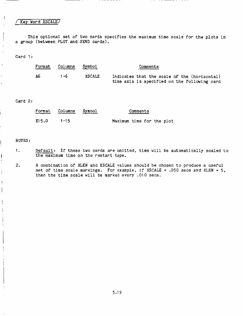
/ Key Word XSCALE/

This optional set of two cards specifies the maximum time scale for the plots in

a group (between PLOT and SEND cards).

Card I :

Format Columns Symbol

A6 1-6 XSCALE

Comments

Indicates that the scale of the (horizontal)

time axis is specified on the following card

Card 2 :

Format Columns Symbol

El 5.0 I-I 5

Comments

Maximum time for the plot

NOTES :

I.

o

Default: If these two cards are omitted, time will be automatically scaled to

the maximum time on the restart tape.

A combination of XLEN and XSCALE values should be chosen to produce a useful

set of time scale markings. For example, if XSCALE = .050 secs and XLEN = 5,

then the time scale will be marked every .010 secs.

5.19

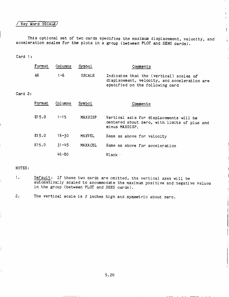
/ Key Word YSCALE/

This optional set of two cards specifies the maximum displacement, velocity, and

acceleration scales for the plots in a group (between PLOT and SEND cards).

Card I :

Card 2:

Format Columns Symbol

A6 I-6 YSCALE

Format Columns Symbol

Comments

Indicates that the (vertical) scales of

displacement, velocity, and acceleration are

specified on the following card

Comments

El 5.0 1-15 MAXDISP

El 5.0 16-30 MAXVEL

E15.0 31-45 MAXACEL

46-80

Vertical axis for displacements will be

centered about zero, with limits of plus andminus MAXDISP.

Same as above for velocity

Same as above for acceleration

Blank.

NOTES :

I.

1

Default: If these two cards are omitted, the vertical axes will be

automatically scaled to accommodate the maximum positive and negative values

in the group (between PLOT and SEND cards).

The vertical scale is 2 inches high and symmetric about zero.

5.20

/ Plot Type/

This required card set specifies which types of plots are desired and the degreesof freedom whose data are to be plotted.

Each card has a key word followed by pairs of node number and degree of

freedom. The key word options are:

DISP

VEL

ACEL

ALL

Plot displacements only for each specified node and degreeof freedom

Plot velocities only for each specified node and degree offreedom

Plot accelerations only for each specified node and degreeof freedom

Plot displacement, velocity, and acceleration for each

specified node and degree of freedom.

Format Columns Symbol Comments

A4 I-4

5-10

14 I5 1 1-80

One of the above key words (start in column I)

Blank

Pairs of: node number followed by its degree

of freedom to be plotted, right justified in

fields of 5 columns each. The degree of

freedom is specified by a number from I through6 where

I denotes global x translation

2 denotes global y translation

3 denotes global z translation

4 denotes global x-rotation

5 denotes global y-rotatlon

6 denotes global z-rotation

NOTES :

I. Any number of these cards can be specified.

5.21

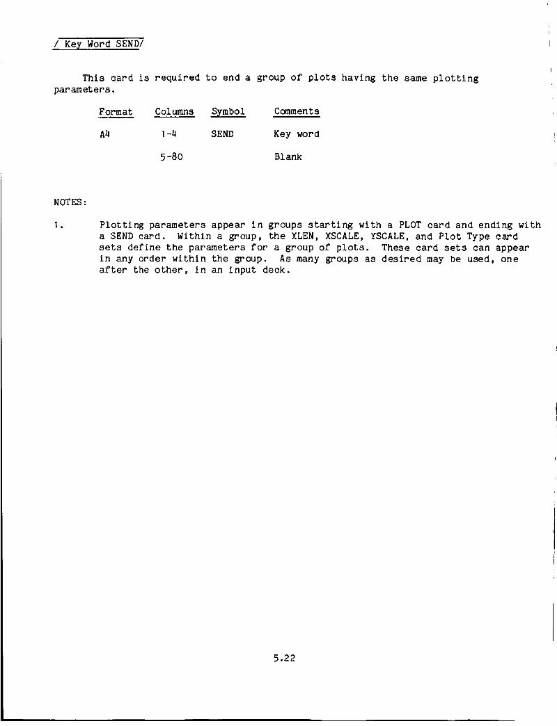
/ Key Word SEND/

This card is required to end a group of plots having the same plotting

parameters.

Format Columns Symbol Comments

A4 I-4 SEND Key word

5-80 Blank

NOTES:

I. Plotting parameters appear in groups starting with a PLOT card and ending with

a SEND card. Within a group, the XLEN, XSCALE, YSCALE, and Plot Type card

sets define the parameters for a group of plots. These card sets can appear

in any order within the group. As many groups as desired may be used, one

after the other, in an input deck.

5.22

/Key Word STOP/

The last card in the input deck must be an alphanumeric STOP left justified incolumns I through 4.

Format Columns Symbol Comments

A4 I-4 STOP Key Word

5-80 Blank

5.23

Example of GRAFIXInputs:

Plot displacement, velocity, and acceleration histories in the global z direction

for node 2000. Useautomatic scaling. Restart ta_e goes from 0-50 msec, with lasttime step 253, and acceleration units are in/sec _.

0........ I ......... 2 ......... 3......... 4 ......... 5......... 6 ......... 7......... 812345678901234567890123456789012345678901234567890123456789012345678901234567890

GRAPHICSTESTPROBLEM- DYNAMICANALYSISOFPLOT 1 253 2ALL 2000 3SENDSTOP

FRAME

A sample plot is shownbelow.

i

Zb-.w

Zo

,,j_-

_rJQ.

_8

V i

• .

'_qll I.o (.

NiN;O.O

'o.ooooo o_ooLoo _'..o(.,.eo_ o_c_sr._ olo_;oo oJoosoo o!oo6_TIME

NOOE 20C0 Z D[SPLi_E.ENT/.

it)

_ ..... -

0.J

> !o}ooooo oJoo:co oJ_z_o o:o,_m o:o_oo oloe_.m

TIME2000 i OISPLR:EMENT

oilI , , , , ,

o ....i':T;;i:'_i;_}:,_,_,rI "_--ST,ni_....q - -

0100._00

TIMENO0( 2000 Z DISPLRCKI'_(NT

oloo_m

B,.aR_IC'_T(_T P_0_LEW - O_'Nn_lt ¢N_,I_IS Of • FIVe(

5.24

6.0 EXAMPLEINPUT

This section contains listings of input data for a number of sample problems.The principal intent in providing these sample inputs is to give the user an overallview of somecomplete representative but simple input decks. Hopefully, these can beused as a supplement to the discussions in Section 3 and 4. Also provided with eachproblem is a brief discussion of results and representative plots of output data.These can serve as benchmark results for program validations.

A detailed picture of the sample problem idealizations showing node and elementlabeling has not been provided. It is suggested that the input plotting programSATELLITEbe used to generate computer plots of the input data, if desired.

6.1

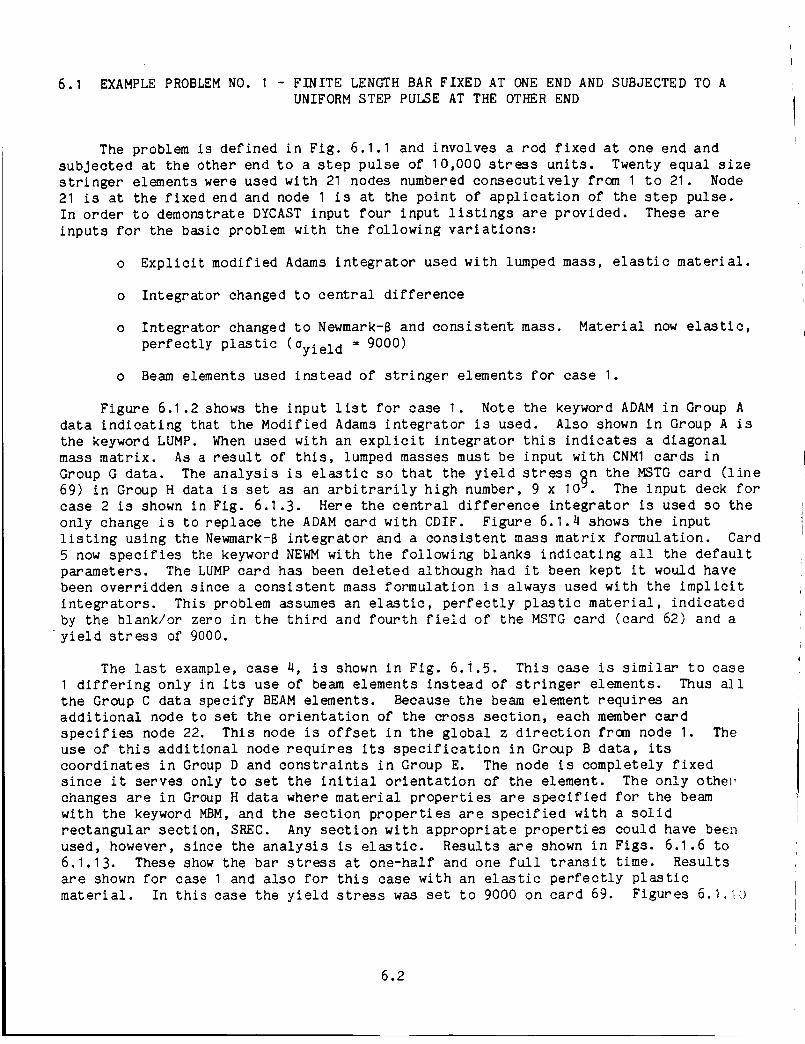
6.1 EXAMPLEPROBLEMNO. I - FINITE LENGTHBARFIXEDAT ONEENDANDSUBJECTEDTO AUNIFORMSTEPPULSEAT THEOTHEREND

The problem is defined in Fig. 6.1.1 and involves a rod fixed at one end andsubjected at the other end to a step pulse of 10,000 stress units. Twenty equal sizestringer elements were used with 21 nodes numberedconsecutively from I to 21. Node21 is at the fixed end and node I is at the point of application of the step pulse.In order to demonstrate DYCASTinput four input listings are provided. These areinputs for the basic problem with the following variations:

o Explicit modified Adamsintegrator used with lumped mass, elastic material.

o Integrator changed to central difference

Integrator changed to Newmark-8and consistent mass. Material now elastic,perfectly plastic (_yield -- 9000)

o Beamelements used instead of stringer elements for case I.

Figure 6.1.2 shows the input list for case I. Note the keyword ADAMin Group Adata indicating that the Modified Adamsintegrator is used. Also shown in Group A isthe keyword LUMP. Whenused with an explicit integrator this indicates a diagonalmassmatrix. As a result of this, lumped massesmust be input with CNMIcards inGroup G data. The analysis is elastic so that the yield stress _n the MSTGcard (line69) in Group H data is set as an arbitrarily high number, 9 x 10J. The input deck forcase 2 is shown in Fig. 6.1 .3. Here the central difference integrator is used so theonly change is to replace the ADAMcard with CDIF. Figure 6.1.4 shows the inputlisting using the Newmark-8integrator and a consistent mass matrix formulation. Card5 now specifies the keyword NEWMwith the following blanks indicating all the defaultparameters. The LUMPcard has been deleted although had it been kept it would havebeen overridden since a consistent mass formulation is always used with the implicitintegrators. This problem assumesan elastic, perfectly plastic material, indicatedby the blank/or zero in the third and fourth field of the MSTGcard (card 62) and ayield stress of 9000.

The last example, case 4, is shown in Fig. 6.i.5. This case is similar to caseI differing only in its use of beamelements instead of stringer elements. Thus allthe Group C data specify BEAMelements. Becausethe beamelement requires anadditional node to set the orientation of the cross section, each membercardspecifies node 22. This node is offset in the global z direction from node I. Theuse of this additional node requires its specification in Group B data, itscoordinates in GroupD and constraints in Group E. The node is completely fixedsince it serves only to set the initial orientation of the element. The only otherchanges are in GroupH data where material properties are specified for the beamwith the keyword MBM,and the section properties are specified with a solidrectangular section, SREC. Any section with appropriate properties could have beenused, however, since the analysis is elastic. Results are shown in Figs. 6.1.6 to6.1.13. These showthe bar stress at one-half and one full transit time. Resultsare shown for case I and also for this case with an elastic perfectly plasticmaterial. In this case the yield stress was set to 9000 on card 69. Figures 6. I._i()

6.2

and 6.1.11 show results for case 3 using the implicit Newmark-B integrator. Figures

6.1.12 and 6.1.13 show results for a 40 element model with linear strain hardening.Here an elastic and plastic wave front is seen.

OA

L=40

E = 1,0 107

p = 2.588 10 .4

20 EOUAL SIZE ELEMENTS

ONE TRANSIT IS 20.35 x 10 -5 $

WAVE SPEED IS: C =

Fig. 6.1 .I Finite Length Bar Fixed at One End and Subjected to a Uniform Step Pulseat the Other End

6.3

CARDCOUNT

i_

2-3-4-5-6-7-8-9-10-11-12-13-14-15-i-_-17-IB-19-3V-

_a

22-.._

25-26-27-2B-

30-Ji-

32-.._

34-35-_¢-

00-

40-,,51-

42-43-44-45-46-

PRO_AN LISTINGOF INPUT_TA CARDS

,.,, ..... 1.... ,,,,,2,.,,o,.,.3..,,.,.,,4,,,,.,,,,5, ........ 6......... 7......... 812_4567_9_1234_6789_1234_67_9_1234567_9_1234567_9_123456789_123456789_1234_67_9_

DYCASTCHECKPROBLEM I UNIFORMBAR STEPPULSELUMPEDMASSELASTICMODIFIEDADAMS,,,

DYNADYNAADAMLUMPTIMEMPRIN

INPRIN

ISEND

ISTRGSTRGSTRGSTRBSTRGSTRGSTRGSTRGSTR6STRGSTRGSTRGSTR6STRGSTRGSTRGSTRGSTRGSTRGSTRGSEHDGRDXGRDXGRDXGRDXGRDX6RDXGRDXC-RDXGRDXGRDXGRDX_DX

0000 5 1001.0 20,5 E-O5 5.00 E-06 0,0,05 ,01 ,0001

-20

-21

-211 I 22 2 33 3 44 4 55 5 66 6 77 7 BG S 99 9 i010 10 Ii11 11 L212 12 1313 13 1414 14 15IS 15 1616 16 i?17 17 IS18 18 1919 19 2020 20 21

0,0 I2.0 n4.0 36,0 4S,O 5IO,C 612.0 714,0 S16,0 918.0 1020.0 1122,0 12

......... i ....... n " 5 6 7 B5 0 _ c 0 _ m _ _ _ _ _ _ 0 _ m _ _ 9 5 r 9I_34567_90134w67B,OI_34_678901_34J6_B901_34o6;B,OI_34_67B90I_34p6,Bgo1_34_6,B90

Fig. 6.1.2 Example Problem No. 1 - Input Listing Case I (Sheet I of 2)

6.4

CARDCOUNT

ISQuALrrY

PROBRAHLISTI_OF INPUTDATACARDS

.........i.....,,..2......,..3.,..,,,,,4....,.,..5.........6,........7.........81234_6789_234_67_9_234_67_9_123456789_1234_67_9_234_67_9_1234_67_9_234_6_89_

47- BRDX 24.04B- BRDX 26.049- ORDX 28.050- BRDX ZO.O51- BRDX 32.052- BRDX 34,053- 6RDX 36.054- ORDX 38.055- 6RDX 40.056- ORDY 0.057- BRDZ 0,0SO- SEND59- SPC 00000060- SPC 10OO006$- SEND62- CNMI 2.5879918E-0463- CNMI64- 1 2165- CNMI 5,1759836E-046_- CNHl67- 2 -2068- SEND69- MSTB I,E770- 0.071- i -2072- SEND73- CONC 1 1,0 E 0474- CONC75- PTHE76- PTME77- SEND78- STOP

1314151617IB1920211 -211 -21

211 -20

I. O. 9. E09

1,0 0,01.0 5.0 E-03

,.,......l,.......,2........,3.,,......4........,5...,,....6...,.....7.........8_234567_9__2_45_7_9__2345_7_9__234567_9__234567_9_1234567_901234_67B9_1234_67_90

Fig. 6.1.2 Example Problem No. 1 - Input Listing Case 1 (Sheet 2 of 2)

6.5

CARDCOUNT

_

3-4-5-6-7-S-9-I0-II-12-13-14-15-16-17-18-19-20-21-

O'I_

24-25-Ol.

2.,=-2B-29-30-31-32-33-34-35-36-37-3S-

40-41.42-43-44-45-46-

PROBRAMLISTINGOF INPUTDATACARDS

.,,o ..... 1,o.o ..... 2......... 3 .... .,.,.4 ......... 5°.°. ..... 6 ......... 7......... 8_23_67_9_2_456789_23456789_234567_9_234567_9_23456789_12345_78?_234_6789_

DYCASTCHECKPROBLEMCENTRALDIFFERENCEINTEGRATOR,..

BYNADYNACDIFLUMPTIMEMPRIN

INPRIN

ISEND

iSTR6STRGSTRBSTRGSTR6STRGSTRBSTRGSTR5STRBSTRBSTRGSTRBSTRGSTRGSTRGSTRGSTRGSTRBSTRGSENDGRDXORDXGRDXGRDXGRDXGRDXGRDXORDXGRDXBRDXGRDXGRDX

0000 5 1001,0

2 UNIFORMBARSTEPPULSELU_ED MASSELASTIC

20.5 E-05 5.00 E-06 0.0

-2O

-21

-211 1 22 2 33 3 44 4 55 5 66 6 77 7 B8 B 99 9 10I0 I0 II11 El 1212 12 1313 13 1414 14 1515 15 1616 16 1717 17 1318 I_ I_19 19 2020 20 21

0.0 I-.0 24,0 36,0 48.0 5I0.0 612.0 "14.016.0 918.0 IC'2O.0 1122.0 12

5 " 7• 2 3_234567@9_234567_9_234_67_9_234567_9_1234567_9_1234567_9_1234_67S9_12345678?_

Fig. 6.1.3 Example Problem No. I - Partial Listing of Input - Case 2

6.6

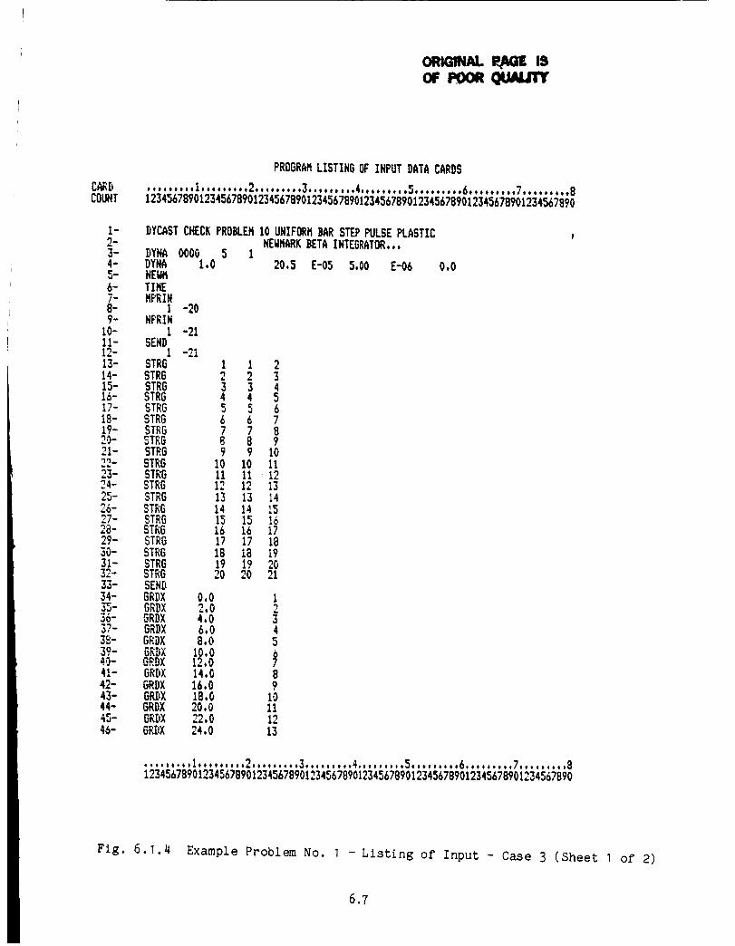
o11 p4tm{IS

CARDCOUNT

PROGRAMLZSTINGOFZNPUTDATACARgS

.,, ...... 1, ........ 2....... .,3 .... , .... 4,.,...,..5 ...... ,..6.,.......7..,, ..... 81234567____234567_9__23456789_123456789_123456789_1234567_9__234567___[234567___

2-3- DYNA4- DYNA5- NEWM6- TIME7- MPRIN8- !9- NPRIN

10- 111- SEND12- I13- STRG[4- STRO15- STROI_- STRG17- STRO18- STRG19- STRG20- STRG21- STRG22- STRG23- STRG24- STRB25- STRG26- STRG27- STRG2B- STRG29- STRG30- STRG31- STRG32- STRG33- SEND34- GRDX35- GRDX36- GROX37- GRDX3_- GRDX39- GRgX4O- GRDX41- GRDX42- GRDX43- ORDX44- GRBX45- GRDX4b- GR_X

DY_ST CHECKPROBLEM10 UNIFORMBARSTEPPULSEPLASTICNEWHARKBETAINTEBRATOR...

0000 5 11,0 20.5 E-05 5.00 E-06 0.0

-2O

-21

-2iI I 22 2 33 3 44 4 55 5 66 6 77 7 88 8 ?9 9 I010 I0 II11 II 1212 12 1313 13 1414 14 !515 15 1616 16 17i) 17 IB18 i8 1919 19 2020 20 21

0.0 12.0 24.0 36.0 48.0 5I0.0 o!2.0 714.0 816,0 ?1B.0 i020.0 1122.0 1224.0 13

.... ,...,1..,..,.,,2 ......... 3......... 4,, ....... 5........ .6.., ...... 7....... ,,8_234567____234_67_9__234567_9__234_67_9__234_6789__23456789__234_67B9__234567_9_

Fig. 6.1.4 Example Problem No. 1 - Listing of Input - Case 3 (Sheet I of 2)

6.7

CARDCOUNT

.., ..... ,1,....,...2,..,...,.3.o,..,..,4...o. .... 5.., ...... 6,.....,..7....,,...81234567B9_123456789_123456789_1234567_9_1234567_9_1234_67_9_1234_6789_123456789_

47- BRDX 26.0 1448- BRDX 28.0 1549- GRDX 30,0 1650- GRDX 32.0 1751- BRDX 34,0 1852- GRDX 36.0 1953- GRDX 3B.0 2054- GRDX 40.0 2155- 6RDY 0.0 156- GRDZ 0.0 157- SEND58- SPC 000000 2159- SPC I00000 I60- SEND61- SEND62- MSTG i,E763- 2,588E-0464- I -2065- SEND66- CONC I 1.0 E 0467- CONC&8- FTHE69- PTME70- SEND71- STOP

-21-21

-2O

I. O. 9. E03

1,0 0.01.0 5,0 E-03

......... i......... 2.... , .... 3 ......... 4......... 5 ......... 6 ....... ..;." ........ 812345678901234567890123456789012345678901234567890123456789012345678901234567890

Fig. 6.1.4 Example Problem No. I - Listing of Input - Case 3 (Sheet 2 of 2)

6.8

ORIGINAL PAGE IcJ

of POORQUAUTY

CARl)COUNT

2-3-4-5-

7-8-9-

10-11-12-13-14-15-16-17-I8-19-20-21-2n-23-24-25-2_-37-2B-29-30-_d

,,)1-

3"-6.

33-34-,35-

3..R-39-t,O-4'=-42-43-44-45-46-

PROGRAMLISTINGOFINPUTDATACARDS

.o. .... ,.1 ...... ,.,2. o. ...... 3...o..,..4,..oo....5.o.o.,o,,6 ......... 7o,,, ..... 81234_6789_1234567_9_123456789_1234567_9_1234_67_9_123456789__234567___123456789_

DYCASTCHECKPROBLEM20 UNIFORMBARSTEPPULSELUHPEDMASSELASTICMODIFIEDADAMSINTEBRATORBEAMELEMENT.,.

DYNADYNAADAMLUMPTIMENPRIN

IMPRIN

IBEND

iBEAMBEAMBEAMBEAMBEAMBEAMBEAMBEAMBEAMBEAMBEAMBEAMBEAMBEAMBEAMBEAMBEAMBEAM_EAMBEAMSENDGRDXGRBXG_XGRDXGRDX_RDXGRDXGRDXBRDXGRDXBRDXGRDX

1 1001.0 20.5 E-05 5.0 E-06 0,0,05 .01 .0001

-21

-20

-221 1 2 222 2 3 223 3 4 224 4 5 225 5 6 226 6 7 22

7 B nnB 8 9 n_9 9 10 2210 10 -11 2211 11 12 2212 12 13 2213 13 14 22

!5 15 16 2216 16 17 2217 17 IB ==n_IB 18 19 2219 19 20 _20 20 21 _n

0.0 I2.0 24.C, 36.0 4e,o 5IC,.O 612,0 714,0 B16,0 91B.0 I020,0 II22,0 12

22

.........I.........2....,....3..,,.,,..4.........5,........6.........7,........B1234567890123456789012345678?01234567890123456789012345678901234508901234567890

Fig. 6.1.5 Example Problem No. 1 - Listing of Input - Case 4 (Sheet 1 of 2)

6.9

CARDCOUNT

PROGRAMLISTINBOF INPUTDATACARDS

......... 1......... 2 ........ ,3..... ,..,4.., ...... 5.,,..,...6 ......... 7 ......... 8_234_67_9__234567_9_1234_67_9_1234_67_9__234_67_9_1234_67_9_1234_67_9_123456789_

47- GRDX 24,C.48- GRDX 26.049- GRDX 28.053- GRDX 30,051- GRDv 32.052- GRDX 34.053- GRD;: 36.054- GRDX 38.055- GRDX 4(..0c'&,_,.- GRDY 0.057- GRIIZ 0.05B- GRDZ 10.059- SENDoC,- SPC OOOO00 I61- SPC 100000 I62- SENDi=_ CNMI 2.5877,°18E-04_m_w

64- CNI4165- i 216_- CNMI 5,1759836E-04#7- CNMI6_- _ -206,°- SEND70- MEM 1.0 E 0771- ", _o_,_.,6E-G4

73- SREC74- J,C' 0,075- i.0 1.0":,,.,-- 1 -2077- SEND7_- CONC 1 1.0 E 0479- CONCr,;i_.- PTME 1.0$I- F'TME I.C$2- SEND_.,_---"STOF

131415161718192021I -22I -21

55

-22-20

0,0

O,O5.0 E-OZ

0.0 0.0 9.0 E 03

......... I ......... 2.... .....o.." ....... 4......... 5 ......... 6......... 7.......... 8l_34_7_901,340678901,34o678901,34_f78901,a406,O,O,a34J678901,a4_6,8901,34u67B,

Fig. 6.1.5 Example Problem No. I - Listing of Input - Case 4 (Sheet 2 of 2)

6.10

STRESS

14,000

12,000

10,000

8OOO

600O

40O0

2OO0

00

MODIFIED ADAMS INTEGRATORAt=5x 10-6s

I I I I '1 r" I I | I

4 8 12 16 20 24 28 32 36 40

LENGTH, in.

E ,, 1.0 x 107

p ,. 2.588 x 10.4

20 EQUAL SIZE ELEMENTS

LUMPED MASS

Fig.

STRESS

6.1.6

14,000

Finite Length Bar Fixed at One End Subjected to a Step Pulse.

Equals One Half Transit. Case I Data Used.

E - 1.0 x 107

p = 2.588x10 4

MODIFIED ADAMS 20 EQUAL SIZE ELEMENTS

At - 5 x 10 -6 s LUMPED MASS

12,000

10,000

8000

6000

40O0

20O0

0 I I I I I I i I I

0 4 8 12 16 20 24 28 32 36 40

LENGTH, in.

Fig. 6.1.7 Finite Length Bar Fixed at One End Subjected to a Step Pulse.

Equals One Wave Transit. Case I Data Used.

Time

Time

6.11

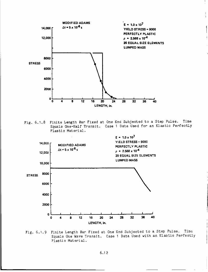
STRESS

14,000

12,000

8OO0

6OO0

4O00

2OOO

MODIFIED ADAMS

At -5x 10"6=E - 1.0 x 107

YIELD STRESS - 9000

PERFECTLY PLASTIC

p - 2.588x10 4

20 EQUAL SIZE ELEMENTS

LUMPED MASS

0 I I I I | --I_1 I I I I0 4 8 12 16 20 24 28 32 36 40

LENGTH. in.

Fig. 6.1.8

14,000

12,000

10,000

STR ESS 8000

6000

4000

20O0

0

Fig. 6.1.9

Finite Length Bar Fixed at One End Subjected to a Step Pulse.

Equals One-Half Transit.

Plastic Material.

MODIFIED ADAMS

At= 5 x 10"65

Time

Case I Data Used for an Elastic Perfectly

E ," 1.0x107

YIELD STRESS = 9000

PERFECTLY PLASTIC

p = 2.588 x 10 -4

20 EQUAL SIZE ELEMENTS

LUMPED MASS

I ! ! I I I I I I I0 4 8 12 16 20 24 28 32 36 40

LENGTH, in.

Finite Length Bar Fixed at One End Subjected to a Step Pulse. Time

Equals One Wave Transit. Case I Data Used with an Elastic Perfectly

Plastic Material.

6.12

STRESS

14,000

12,000

10,000

NEWMARKZ_t- 5 x 10"6s E I 1.0x 107

p = 2.588x I0"4

20 EQUAL SIZE ELEMENTS

CONSISTENT MASS

8OOO

6OOO

4OOO

2000 -

0

40

LENGTH, in.

Flg. 6.1.10 Finite Length Bar Fixed at One End Subjected to a Step Pulse. Time

Equals One-Half Transit. Case 3 Data (Elastic).

STRESS

14,000

12,000

10,000

80O0

6O0O

4OOO

2O0O

NEWMARK

Lit ,, 5 x I0-6 s

^ _ A A A _I v V V V _

E ,, 1.0 x 107

p = 2.588 x 10 -4

20 EQUAL SIZE ELEMENTS

CONSISTENT MASS

0/ I I I I I. I I I I

0 4 8 12 16 20 24 28 32 36 40

LENGTH, in.

Fig. 6.1.11 Finite Length Bar Fixed at One End Subjected to a Step Pulse. Time

Equals One Wave Transit. Case 3 Data Used (Elastic).

6.13

14,000

12,000

10,000

8OOO

STRESS

6OOO

_000

2OOO

00

MODIFIED ADAMS

At = 2.5 x 10.6 =

" w

PLASTIC /WAVEFRONT

E = 1.0 x 107

LINEAR STRAIN HARDENING

ET/E - 0.1YIELD STRESS = 9000

p = 2.588x 10 -4

40 EQUAL SIZE ELEMENTS

• I

ELASTIC/_

WAVEFRONT

I I I I A I I I I

4 8 12 16 20 24 28 32 36

LENGTH, in.

4O

Fig. 6.1.12 Finite Length Bar Fixed at One End Subjected to a Step Pulse.

Equals One-Half Transit. Forty Equal Sized Elements Used and

Linear Strain Hardening.

Time

14,000

12,000

10,000

STRESS

80OO

6OOO

°I2OOO

00

Fig. 6.1.13

MODIFIED ADAMS

At = 2.5 x 10-6 =

PLASTICWAVEFRONT

E = 1.0 x 107

LINEAR STRAIN HARDENING

ET/E = 0.1YIELD STRESS = 9000

p = 2.588 x 10 -4

40 EQUAL SIZE ELEMENTS

ELASTIC

_ WAVE

FRONT

/

I J I . t _1_ I I I A I

4 8 12 16 20 24 28 32 36 40

LENGTH, in.

Finite Length Bar Fixed at One End Subjected to a Step Pulse.

Equals One Wave Transit. Forty Equal Sized Elements Used and

Linear Strain Hardening

6.14

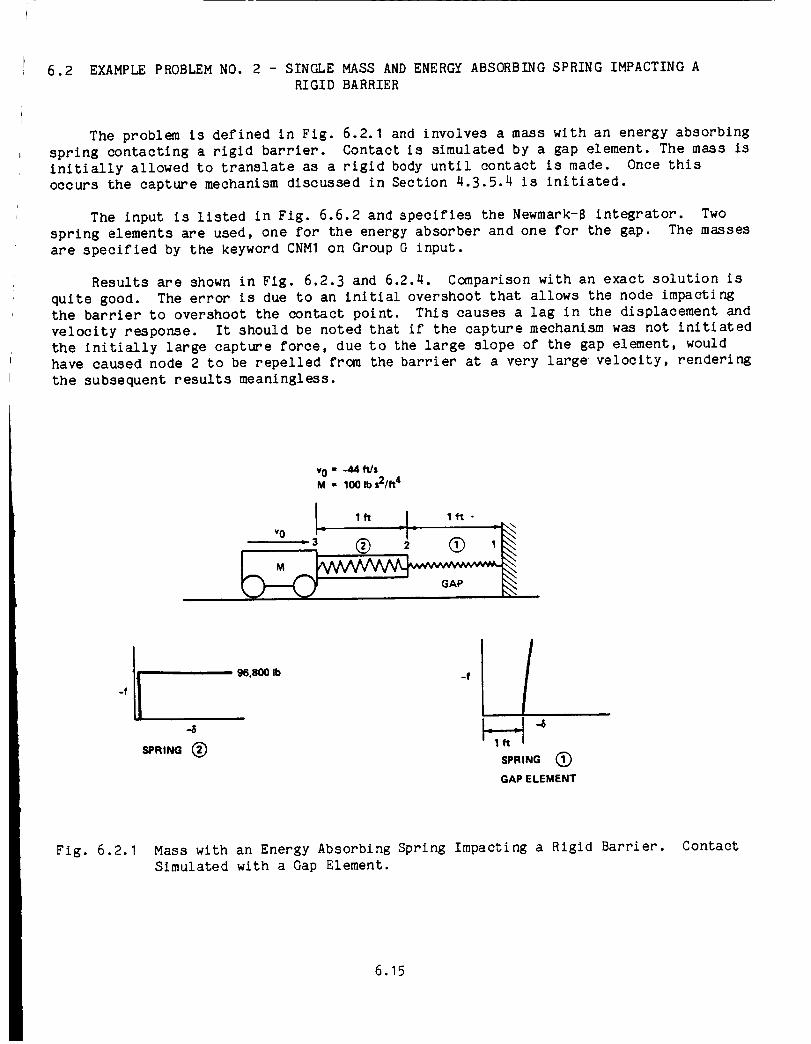
6.2 EXAMPLEPROBLEMNO. 2 - SINGLEMASSANDENERGYABSORBINGSPRINGIMPACTINGARIGID BARRIER

The problem is defined in Fig. 6.2.1 and involves a mass with an energy absorbingspring contacting a rigid barrier. Contact is simulated by a gap element. The mass isinitially allowed to translate as a rigid body until contact is made. Once thisoccurs the capture mechanismdiscussed in Section 4.3.5.4 is initiated.

The input is listed in Fig. 6.6.2 and specifies the Newmark-Bintegrator. Twospring elements are used, one for the energy absorber and one for the gap. The masses

are specified by the keyword CNMI on Group G input.

Results are shown in Fig. 6.2.3 and 6.2.4. Comparison with an exact solution is

quite good. The error is due to an initial overshoot that allows the node impacting

the barrier to overshoot the contact point. This causes a lag in the displacement and

velocity response. It should be noted that if the capture mechanism was not initiated

the initially large capture force, due to the large slope of the gap element, would

have caused node 2 to be repelled from the barrier at a very large velocity, rendering

the subsequent results meaningless.

v0 = -44 f',J$M = 100 Ib s2/ft 4

-f

96.800 Ib _f

J.-6

lft

SPRING (_

GAP ELEMENT

Fig. 6.2.1 Mass with an Energy Absorbing Spring Impacting a Rigid Barrier. Contact

Simulated with a Gap Element.

6.15

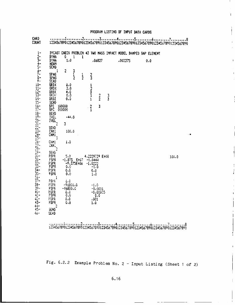
CARDCOUNT

PROGRAMLISTINGOF INPUTDATACARDS

.........1.........2.........3.........4.........5.........6.........7.........B1234567___1234567_9_1234567_9_1234567___1234_67_9_1234567B9_1234_6_8__1234567_?_

DYCASTCHECKPROBLEM43 TWO MASSIMPACTMODELDAMPEDGAP ELEMENTDYNA 0 i 1DYNA 1.0 .06827 .002275 0.0NEWMSEND

i 2 3SPNG i iSPNG 2 2SENDBRDX 0.0GRDX 2.0BRDX 4,0GRDf 0,0GRDZ 0.0SENDSPC 100000SPC 000000SENDIVEL -44.0IVEL

3SENDCNKI 100.0CNMI

3CN_I 1,0CNM:

SENDPSPR S,OPSPR -I,875 E÷07PSPR -9,375E+06PSPR 0,0PSPR 0,0PSF'R 0,0

1

PSPR -96B00,0PSF'R -96800,0PSFR 0,0PSP_ 0,0?SPR 0.0F'SPR 0.0

2SENDSE_D

I23I 2 3I 2 3

4.,==%= E÷OB-I,0444-i.0222

-1.00.0i,0

-I,0-0,')001-0. VVVV.,

0.0.0011.0

100,0

• q......... _......... 2......... 3 ......... 4 ......... S,, ....... 6 ......... ; ......... @_234_7B_1234_67_9O_234_6789_234_67_9_2345_7_9_234_67_9_234_67_234_67_

Fig. 6.2.2 Example Problem No. 2 - Input Listing (Sheet I of 2)

6.16

P

CAR_COUNT

47-

PROGRAHLISTINGOF INPUTDATACARDS

......... I.....,...2.,...,,,.3 ...... ...4........,5 ......... 6 ......... 7 ......... 8_23456789__23456789__23456789__23456789__23456789_123456789__23_567_9__23456789_

STOP

.........i...... n _ ,.,.4.... 5., ,6. ..7........8ote_tte°t_eo_tet*t ,tett teeee° °erect *

_23456789__234S6789__23456789_1234_6789_1234_678___23456789__234_67_9_1234_6789_

Fig. 6.2.2 Example Problem No. 2 - Input Listing (Sheet 2 of 2)

6.17

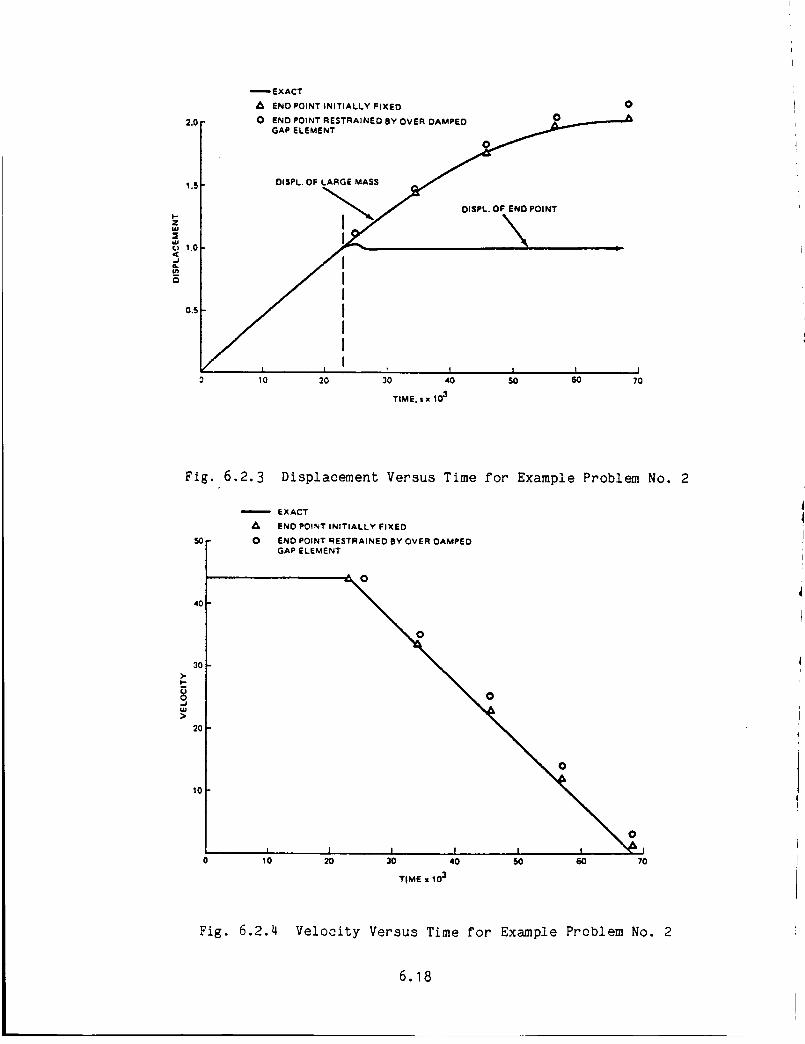
2.0

1.5

Z

,) 1.0<

e_

o.s

_EXACT

A END POINT INITIALLY FIXED

O END POINT RESTRAINED BY OVER DAMPED O

°ii:ioliioss

I I ' I I I

10 20 30 40 ,SO 60

TIME. s x 103

170

>.t-.

Fig.

5O

4O

3O

2O

I0

I

0 10

6.2.3 Displacement Versus Time for Example Problem No. 2

EXACT

END POINT INITIALLY FIXED

O END POINT RESTRAINED BY OVER DAMPED

GAP ELEMENT

0

0 0

I I I I i20 30 40 50 60 70

TIME x 10 3

Fig. 6.2.4 Velocity Versus Time for Example Problem No. 2

6.18

6.3 EXAMPLEPROBLEMNO. 3 - UNIFORMLYLOADEDRESTRAINEDBEAM

The problem is defined in Fig. 6.3.1 and involves a restrained beam, clamped atits edges and subjected to a uniform lateral load. Ten beamelements are used forhalf the beam. The input listing is shown in Fig. 6.3.2. Note that since it is astatic analysis the keyword STATis used in Group A data. The applied load is inputusing the beamload keyword, BMLOin Group I data. However, static loads stillrequire that the table of load factor versus time be specified. For static analysesthe time can be interpreted as a parameter. In the input shown, the maximumloadfactor is 100 with a time step of 16. This leads to a load'step of 960 and a totalload of 6000 since the unit values as prescribed on the BMLOinput is 60. Results areshown in Fig. 6.3.3 and 6.3.4. These figures show the central deflection and axialload versus applied load. Results are plotted for two loads steps, AP = 960 and AP =

240. In both cases, they compare identically with an exact solution. Results are

also shown (Fig. 6.3.5 and 6.3.6) for the case in which the edges are simply

supported. The only change in input for this case is card 35 (Fig. 6.3.2) defining

the SPC for node I. Results are shown for AP = 60 and AP --240. There is, however, a

fundamental difference in the solution. In the clamped case the slope of the load

versus deflection curve, as the beam deforms into the nonlinear range, changes

gradually frcm the initial linear slope. The analysis consequently requires a number

of iterations through this region until the flat portion is reached. However, as seen

in the simply supported case (Fig. 6.3.5), the change in slope in this region is more

pronounced. Consequently, no matter how many iterations are allowed, the solution

does not converge until the step size has been reduced to AP = 60. This step is

required through the highly nonlinear region after which it increases to the

prescribed maximum value. Because of this, an iteration limit was taken as 10 so that

unnecessary calculations would not be performed in the highly nonlinear region.

Again, results compare identically with an exact solution.

L ,,60

AREA " 1.2

MOMENTOF iNERTIA - 0.1

E " 1.0 x 107

10 ELEMENTS IN 1/2 BEAM

Fig. 6.3.1 Uniformly Loaded Restrained Clamped Beam - Static Analysis

6.19

CARDCOUNT

PRO6RAMLISTINBOF INPUTDATACARDS

I _ 3 4 5 6 7$;totff0t to|_oOtff_#ffftfocf tloe000$$ _ottf#fft #fff4fot_ fo&$l$$o$ #$$_t#_

_234567S_2345_78?_12345_7B?_12345_7_?_12345_7_9_12345_7_9_1234567_9_123456789_

DYCAST_MMPLEPROBLEM26BUNIFORMLYLOADEDCLMPEDRESTRAINEDBEAM_TAT,..ELASTICDYNA 0000 IDYNASTATTIMEEEHD

,_ -12BEAM iBEAM 2BEAM 3BEAM 4_EAM 5BEAM 6BEAM 7BEAM 8 _,BEAM ? ;'_.EAM i0 I0r.- i.,",."_[I

_RDX 0.0 E C'C,

GRI.O: _,0 E O0GgDX 9.0 E O0GRDX 12,0 E O0GRD'_ 15.0 E O0G_DX i_.O E C,OGF;D_x 2i.0 E O0GF;;tX 24 '; '".;,_

GFii_X _O,C E O0I.__IIZ 0,0 E 0"_'

GFc3Y 0,'..', E ".'0G_[i'_' 1(;.0 E 0(,SENI_SF'COC,O000SF'C C,'O00,_-_,..... : ,",'_,",1,",

,.i_ I.C-

,: -I0TW[,

0,0

i -t',"SE_D

II00.0

I 2 123 12

3 4 124 5 12.5 ,_ 126 7 127 8 12

) 12I0 12Ii 12

I 12"I

4

67E,

ICiii -i2i -Ii12

12)

-I0ii

E 07 ._"C,,O

0.0 0.01.0 $,C

16.0 0.0,01 25.0

_.C E ":_

• 2 " 4 5 6 "123456,78;O12345678901234567B?O1234567890123456,TBgO1234567890123456787012345_7B(;0

Fig. 6.3.2 Example Problem No. 3 - Input Listing (Sheet 1 of 2)

6.20

CARl!COUNT

PROGRAMLISTINGOFINPUTDATACARDS

. ........ I ......... 2 ......... _ ......... 4 ......... 5 ......... 6 ......... 7 ......... 8

_234_67_9__234567_9__234_67_9__234567_9__234_67_9_123_567_9_1234_67_9_1234_67_9_

47- BMLO 0.0 0,04_- I -I049- PTHE 0.0 0.050- PTHE 100,0 100.0-,_'- SEND52- STOP

-I,0 -I.0

! 2 = 4 5 " 7 O1234567B9_1234567B_1234567B9_234567B9_1234567B_1234_67_9_1234_678_123456789_

Fig. 6.3.2 Example Problem No. 3 - Input Listing (Sheet 2 of 2)

6.21

CENTRAL

DEFLECTION, in.

3.0

2.5

2.0

1.5

1.0

0.5

L" 60in.

t ,, 1 in.

E - 107 psi

I = 0.1 in, 4

A - 1.2 in. 2

10 ELEMENTS IN HALF BEAM

EXACT SOLUTION

+ DYCAST Z_ = 240 Ib

A DYCAST L_P = 960 Ib

1000 2000 3000 4000 5000 6000

LOAD, Ib

Fig. 6.3.3 Uniformly Loaded Restrained Clamped Beam - Central Deflection

Versus Load

30

25

20

AXIAL 15FORCE x 10 -3

10

5

0

t i t _ _ t t _ ½ t 1_ _ EXACT SOLUTION

L _- + DYCAST ZIP = 240 Ib

L = 60 LI DYCAST Ap = 960 Ib

t =1

E = 107

1=0.1

- I I I I I1000 2000 3000 4000 5000 6U00

LOAD, Ib

Fig. 6.3.4 Uniformly Loaded Restrained Clamped Beam - Axial Force Versus Load

6.22

CENTRALDEFLECTION. in.

3.0

2.5

2.0

1_,

1.0

0.5

;= L =3 -- EXACT SOLUTION& DYCAST LIP" 60 Ib

L 7 60in. & LIP- 2401bt - 1 in. ITERATION LIMIT - 10E - 107 psi

I " 0.1 in.4

| I I | I /

0 1000 2000 3000 4000 5000 6 000

LOAD, Ib

Fig. 6.3.5 Uniformly Loaded Restrained Simply Supported Beam - Central

Deflection Versus Load.

AXIAL FORCE x 10 .3

30

25

2O

15

10

5

0

-- EXACT SOLUTION& DYCAST _P =60 Ib

, . =' A AP=2401b,_- t. I ITERATION LIMIT "=10

L" 60in.

t =1in.

E = 107 psi]_ - 0.1 in.4A = 1.2 m2

10 ELEMENTS

• I I I I I I

1000 2OO0 3OOO 4OOO 5OO0 6OO0

LOAD, Ib

Fig. 6.3.6 Uniformly Loaded Restrained Simply Supported Beam - Axial

Force Versus Load

6.23

6.4 EXAMPLE PROBLEM NO. 4 - IMPULSIVELY LOADED CLAMPED BEAM

The problem is defined in Fig. 6.4.1 and involves a rectangular section beam,

clamped at both ends, with an impulsively applied load on the center section simulated

by an applied initial velocity. The listing of the input is in Fig. 6.4.2. _Note the

following: A maximum time is set at 1.2 msec with a time step of 10.0 x 10 -6 sec.

The analysis uses the Newmark-8 integrator. Member outputs are to be printed for only

I, 2, and 10. Initial velocities are specified in Group F data with the keyword

IVEL. The material is elastic, perfectly plastic with a yield stress of 4.14 x 104

psi.

Figure 6.4.3 sho_s the results of central deflection versus time. For At -- I0 x10 -6 and At = 2 x 10 -_ s. Figure 6.4.3 indicates that the results are in essential

agreement with the maximum differences at later times. The results with the smaller

of the two time steps compares favorably with results presented in "Finite Element

Analysis of Large Transient Elastic-Plastic Deformations of Simple Structures with

Applications to the Engine Rotor Fragment Containment/Deflection Problem," MIT ReportASRL TR 154-4 (1972). It should be noted that results for the two different time

steps agree at early times because the initial__onlinearities as seen in Fig. 6.4.3caused the time step to be reduced to 2.5 x 10 _ s in that region.

v0 - 5000 in./$ /, 10 in. ,

A - 0.15 in.2

I - 1.953x10 4in. 4E - 1.04 x 107Ib/in.2

p " 2.5 x 10.4 Ib $2/in.4

10ELEMENTS IN 1/2 BEAM

Fig. 6.4.1 Impulsively Loaded Clamped Beam

6.24

CARDCOUNT

i.

2-3-4-5-6-I-

8-9-10-ii-12-i7.

14-15-15-17-18-IT-20"21-

")."X-

24-

26-27-

2%30-31-32-_,.%-

34-35-3_-,%/-

38-3.0-40-41-

44-45-

ORIGINAL PAGE IS

OF POOR QUAUTY

PROGRAMLISTINGOF INPUTOATACARDS

.........I..,,.....2.,.......3.........4.........5.........6.........7.........81234567890123456789012345678901234567B?Oi2345678?O12345678901234567BgO1234567890

DYCASTEXAMPLEPROBLEM37AIMPULSIVELYLOADEDBEAM (WU- WITMER)NEWMARKINTEGRATOR.,.

DYNA 0000 40 1000BYNA 1.0 1,2 E-03 10.00E_6NEWM .25 .5 .01CONMTIMEMPRIN

i 2 10NPRIN

1 -12SEND

i -12BEAM 1 1 2 12BEAM 2 _ o 12BEAM 3 3 4 12BEAM 4 4 5 12BEAM 5 5 6 12BEAM 6 6 7 12BEAM 7 7 B 12BEAM 8 B ? 12BEAM 9 9 i0 12BEA_ i0 I0 ii 12_NDGEIIX O,0 i 12

G_DX .5GRDX 1.0

GRDX 2.0 5GRDX 2,5 6_RDX 3,0GRDX 3,5 BGRDX 4.0 9GRDX 4,5 i0GRDX 5.0 iiG_In 0,0 I -IIGRDY 1.0 12GRDZ 0.0 1 -12SENDSPC 001000 1SPC I01010 2 -i0SPC 000000 11 12SENDiVEL 0.0 0.0 -.5 E+04!VEL

1 2

0.03.0

- PLASTIC ,

• _ 3 5 6 7 B4_,.o.._,_.,*.te_i._.,.me, .._..t,..4.o.,,*,$, tt_t*om_. ...,,t_,. ...Omm,.m

1234567_234567_9_234567_9_1234567_9_1234567_9_1234567_1234_67_1234567_

Fig. 6.4.2 Example Problem No. 4 - Input Listing (Sheet 1 of 2)

6.25

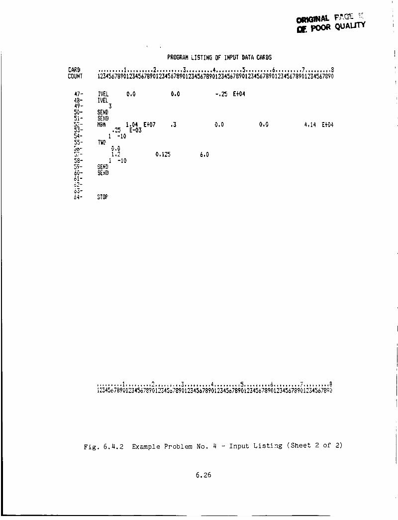
CARDCOUNT

poor qUAL.n

PROGRAMLISTINGOF INPUTDATACARDS

.........I..,,,..,.2.....,,..3.........4.........5.........6.........7.........81234567BgOI23456_goI234567BgOI234567BgOI234567B?OI234567BgOI234567Bg01234567890

47- IVEL O.O4@- IVEL49- 35O- SEND51- SEND52- MBM 1.0453- .25 E-0354- I -I055- TWD3o- 0.0

58- 1 -i05_- SEND60- SEND61-_-

63-_4- STOP

O.O -.25 E÷04

E÷07 .3 0.0 O.O 4,14 E÷04

0.125 6.0

I 2 " 4 5 ' " 8_234567_?_2_45678?_2345_7_9_234567_?_2_45_7_?_12345678_1234567_?_2345_7B9_

Fig. 6.4.2 Example Problem No. 4 - Input Listing (Sheet 2 of 2)

6.26

CENTRALDEFLECTION, in.

-0.8

-0.7

-0.6

-0.5

-0.4

-0.3

-0.2

-0.1

0"0

f vy -. ...... Lit - 2 x 104s$ Zl

r Wu - WITMER 0

_L=-.-_ 10 in...._.-,_

v0 = -5000 in.is

I I I i I i0.2 0.4 0.6 0.8 1.0 1.2

TIME, $ x 103

Fig. 6.4.3 Central Deflection Versus Time for Example Problem No. 4

6.27

6.5 EXAMPLEPROBLEMNO. 5 - IMPULSIVELYLOADEDELASTO-PLASTICRECTANGULARPLATE

The problem is defined in Fig. 6.5.1 and involves a rectangular plate subjectedto an impulsively applied lateral velocity. The listing of the input is in Fig.6.5.2. Thirty plate elements (TRP2) are used in one quarter of the plate_ A constantstep central difference integrator is used with a time step of 0.25 x 10-v s. Amaterial w_th linear strain hardening is used with ET/E = 0.005 and a yield stress of233.0 N/ram_. Eight integration layers were prescribed through the plate thickness.Results are shown in Fig. 6.5.3 and compare favorably with results given in "TransientDynamic Large Deflection Analysis of Elastic Viscoplastic Plates by the Finite ElementMethod," Int. J. Mech. Sci., Vol 22, pp 151-166 (1980).

iv

L

B

L = 128.59 mm p = 7.72 x 10 .9 N s2/mm 4

B = 76.2 mm YIELD STRESS = 2.33 x 102 N/mm 2

THICKNESS = 2.499 turn E = 2.07 x 105 N/ram 2

v=0.3

Fig. 6.5.1 Impulsively Loaded Elasto-Plastic Rectangular Plate

6.28

ORlelNAL ISOF POOR QUALITY

CARDCOUNT

2-3-4-5-6-i-

8-9-

10-Zl-12-13-14-15-16-:'7_

',O-

1g-20-21-

__

'3.¢.. _

29-30-_a

32-_3-

34-35-30-

_?-- .-..-

40-41-42-43-44-45-46-

PROBRAHLISTIN6OF INPUTDATACARDS

.... . .... 1,... ..... 2 ......... 3.,, ...... 4......... 5......... 6....... ..I." ........ 81234_6789_234_6789_234_67_9_234567_9_234_67_9_234567_9_123456789_23456789_

DYCASTEXAMPLEPROBLEMDYNA 0000 80 1000DYNACDiFTIMEMPRIN

1 2NPRIN

i -24SEND

I -24TRP2 i I 5 6TRP2 2 6 2 iTRF'2 3 2 6 7TRF'2 4 7 3 2TRP2 3 3 7 @TRP2 6 8 4 3TRP2 7 S 9 i0TRP2 8 10 6 ST_F'2 9 6 10 11TRF'2 I0 ii 7 6TRP2 ii 7 II 12TRP2 12 12 B 7TRP2 13 9 13 14TRP2 i4 14 10TRP2 15 10 14 15TRP2 16 15 11 I0TRP2 17 11 15 16TRF'2 IB I_ 12 IiT_P2 19 13 17 18TRP2 20 18 14 13TRP2 21 14 18 19TRF'2 22 19 15 14TRP2 23 i5 19 20TRP2 24 20 16 15TRP2 25 17 21 22T_F'2 ".'622 18 17TRP2 27 18 _ ._3TRP2 28 23 I? IBT_P2 29 19 23 24TRP2 30 24 20 I?SEND6RDX 0.0 E+O0 t -4ORDX 1.2B59 E+0! 5 -BGRDX 2,571B E+01 9 -12GRDX 3.8577 E+OI 13 -16

IMPULSIVELYLOADEDCLAMPEDPLATE

0.400 E-O3 0.250 E-O&

............ _..... ,,,.4 ......... 5 ......... 6 ......... 7......... 8_234_67_9__234567____234567____2_45678___234_6789__234_678?__234567____234567_9_

Fig. 6.5.2 Example Problem No. 5 - Input Listing (Sheet 1 of 2)

6.29

ORIGINAL P._GE IS

OF POOR QUALITY

CARDCOUNT

47-4,3-4(;-

52-

5.O-

6,--

_.,_

,DT-

"? _,-

i-

.2-72_

"__-,j_..,..

PROGRAM LISTING OF INPUT OATA CARDS

! n 3 4 5 6 7 8IoeettoQ_ _*ootoolt&o&oft$ftt oootooott totoot_lo &ottltoo* t*_*$t_ _,,_,

_234567_9_12345678_12345678_23456789_2345678_12345678_123456789_2345678_

GRDX 5,1436 E+01 17 -20GRDX 6,4295 E÷01 21 -24G_liY 0,0 E÷O0 I -4 -21GRTiY 1,27 E÷01 n -4 -o')GRDY 2.54 E÷01 3 -4 -23,GR[,Y3.81 E+01 4 -4 -24GRZ_Z 0.0 E÷O0 I -24SENTi_.-.._r_, C,OI",O0 1_FC C'III00 n 3_i'_" 111110 6 -4 -18or:. 111110 / -4 -I_SF'C :-00000 4 -4 -20SPC 101010 5 -4 -17SFC OC'O0'}O 21 -24.,c_iil_:::'_LC'.O E+O0 0.C' E.O? ".C.45 E÷04::."EL0,0 E+O0 0.0 E+O0 0.0 E÷O0

I -24_EH_.::_ATI .....;.:,' E+05 ,":.,,__'_ E-09,}.}05 0.0 '__"

: -3,3THII_ 2,499 S.O

I -30

, "%E'rO.

r_ ¸,,T._,F

' 3 4 5 " 7.=_4uo8,vl=34_6789Cl,o4u6789Ol_34ue7890I=_4uG,Bg_l=a,_b,B,Ol_4uG,_u1_o_,_:_

Fig. 6.5.2 Example Problem No. 5 - Input Listing (Sheet 2 of 2)

6.30

CENTRAL DEFLECTION

v0 ,, 7.045 x 104 mm/=

wc (ram)

15

10

0

(3 TRP2 CENTRAL DIFFERENCE INTEGRATOR

At = 0.5 x 10 _ =

REFERENCE F.E. SOLUTION

EXPERIMENT

I I I I I I I I I I =40 80 120 160 200 240 280 320 360. 400

TIME, _s

Fig. 6.5.3 °Central Deflection Versus Time for Example Problem No. 5

6.31

Standard Bibliographic Page

1. Report No.

NASA CR-40404. Title and Subtitle

DYCAST-- A Finite Element Program for theCrash Analysis of Structures

2. Government Accession No.

7. Author(s)

A. B. Pifko, R. Winter, and P. Ogilvie

9. Performing Organization Name and Address

Grumman Aerospace CorporationBethpage, NY 11714

12. Sponsoring Agency Name and Address

National Aeronautics and Space AdministrationWashington, DC 20546

3. Recipient's Catalog No.

5. Report Date

January 1987

6. Performing Organization Code

8. Performing Organization Report No.

10. Work Unit No.

11. Contract or Grant No.

NASI-1314813. Type of Report and Period Covered

Contractor Report

14. Sponsoring Agency Code

505-63-41-01

15. Supplementary Notes

Langley Technical Monitor:Final Report

Martha P. Robinson

16. Abstract

DYCAST is a nonlinear structural dynamic finite element computer codedeveloped for crash simulation. The element library contains stringers, beams,membrane skin triangles, plate bending triangles and spring elements. Changingstiffnesses in the structure are accounted for by plasticity and very largedeflections. Material nonlinearities are accommodated by one of three options:elastic-perfectly plastic, elastic-linear hardening plastic, or elastic-nonlinearhardening plastic of the Ramberg-Osgood type. Geometric nonlinearities arehandled in an updated Lagrangian formulation by reforming the structure into itsdeformed shape after small time increments while accumulating deformations,strains, and forces. The nonlinearities due to combined loadings are maintained,and stiffness variation due to structural failures are computed. Numericaltime integrators available are fixed-step central difference, modified Adams,Newmark-beta, and Wilson-theta. The last three have a variable time stepcapability, which is controlled internally by a solution convergence errormeasure. Other features include: multiple time-load history tables to subjectthe structure to time dependent loading; gravity loading; initial pitch, roll,yaw, and translation of the structural model with respect to the global system;a bandwidth optimizer as a pre-processor; and deformed plots and graphics aspost-processors.

17. _ey_or_(Sugges_dby Authors(s))brasn anasyslsDynamic Analysis

Nonlinear Analysis

Large Displacement Analysis

Finite Element Analysis

19. Security Cl_sif.(of this report)

Unclassified

18. Distribution Statement

Unclassified-Unlimited

Subject Category 64

20. Security Cla_sif.(of this page) 21. No_of Pages 22. PriceUnclassified 348 A15

For sale by the National Technical Information Service, Springfield, Virginia 22161NASA-Langley, 1987