Hypothesis testing via classifier performance with an appli-cation to identifying Drosophila larval behavioral “mutants”

Rebeca Salas-Boni∗1 , Tomoko Oyama2 , Marta Zlatic2 and Esteban Tabak.1

1Courant Institute of Mathematical Sciences, New York University, New York, NY 10012.2Janelia Farm Research Campus, Howard Hughes Medical Institute, Ashburn, VA 20147, USA.

Email: salasboni@cims.nyu.edu; oyamat@janelia.hhmi.org; zlaticm@janelia.hhmi.org; tabak@cims.nyu.edu;

∗Corresponding author

Abstract

Background: Traditional methods for deciding whether two populations are distinguishable or not often

make assumptions on the distribution of the data, and use these to measure dissimilarity. In this article a novel

approach is proposed, where the performance of classifiers - namely, their accuracy or MSE - is used to determine

whether two populations are distinguishable or not.

Results: An algorithm for evaluating the statistical significance of a measurement of the performance of

a classifier (accuracy, MSE) given in cross validation is devised and implemented. An application to detecting

Drosophila larval behavioral “mutants” in reaction to external stimuli (vibrations) is presented, as well as an

interpretation of the results and comparison with previous findings.

Conclusion: A novel algorithm for hypothesis testing based on the performance of classifiers has been

proposed. It is non-parametric, as well as flexible in allowing the user to determine which classifier to use and which

measure to evaluate performance. We applied our methodology to identifying Drosophila larval populations that

have defective responses to vibration. With our method, we found that the populations of larvae with inactivated

vibration sensing neurons were significantly different to controls. This is consistent with previous findings about

such larval populations.

1

Background

Deciding whether two populations are distinguishable or not is a very common problem in statistics. Exam-

ples include detecting the difference in response to treatment to a new drug between placebo and medicament

patients or detecting differences in behavior between animal populations with distinct neurological disor-

ders. Framing this problem in terms of hypothesis testing, one usually measures selected quantities from

both populations, and determines whether the difference between these quantities is significant or not. Here

we propose a different approach. If the difference between the two populations could be detected, one could

train a classifier on the data, and measure its performance. The accuracy of the classifier – that is, the pro-

portion of correctly classified samples – would be higher if the data sets were intrinsically distinct, whether

two very similar data sets would yield a poorer performance.

In our approach, the null hypothesis H0 – that we cannot detect a difference between both populations with

the given measurements – is to be rejected for a sufficiently small p–value P . We present a study where the

empirical distributions of the accuracy of the classifier under the null hypothesis H0, and the p–value P ,

are estimated via Monte Carlo simulations. We study the results yielded by the most commonly used and

widely available classifiers.

Our methodology is then applied successfully to a data set describing behavioral features of distinct pop-

ulations of fruit fly Drosophila larvae. The fruit fly larva has around 1000 different neural classes, but

the function of most of these classes in behavior is not known. By using genetic methods [5, 9], one can

selectively deactivate single neuron classes of the larvae and identify classes whose inactivation affects a

particular behavior of interest. In this way it is possible to identify a functional set of neurons involved in a

specific behavior which forms a basis for understanding how neural circuits control behavior. The problem

that arises is that of identifying whether a population of larvae with a specific neuron inactivated behaves

significantly different from the control group.

Methods

Initially, a set of observations corresponding to the “wild type” - larvae that have no neurons inactivated

- is given. We are also presented with observations from “mutant” populations, with specific neurons

inactivated. Let us call these data sets Cw and Cm. The task at hand is to determine whether the two

populations exhibit a significantly different behavior or not. If they do, it is said that the “mutant” class is

a “hit”. Our statistical null hypothesis H0 will be that a difference between both classes cannot be detected

2

with the given measurements. That is, we want to test:

H0 : Cw and Cm are indistinguishable

We have to specify what we mean by two sets of observations being distinguishable or not. The benchmark

methods consist in fitting a parametrized distribution to both sets, for example, a Multivariate Gaussian

density, and then measuring the distance between their parameters, say, the difference between the means.

Another approach is to fit a probability density to both sets, not necessarily parametric, and measure the

distance between both probability distributions. In this article we propose a measurement for quantifying

how distinct two populations are based on classification. The methodology is developed in the following

sections.

Differentiating between populations using classifiers

In the context of our problem, each element in the data set is composed by a vector containing all the given

measurements, and a label, either “wild type” or “mutant”. Let us divide the data set randomly into two

disjoint sets: a training set and a test set.

A classifier uses both the measurements and labels in the training set to find a decision boundary that

separates both populations as well as possible, dividing the space into two regions. Afterwards, the

classifier will be able to assign a label to an observation in the test set. The performance of a classi-

fier may be measured by the proportion of samples in the test set it labels corrrectly. This procedure is

referred to as cross validation, and the measurement described is the accuracy A, obtained as in Algorithm 1.

Algorithm 1 Computing the accuracy A

1. Randomly partition the dataset into two parts: a training set and a test set.

2. Train the classifier on the training set.

3. Compute the accuracy A, that is, the proportion of correct classified samples in the test set, using theclassifier trained in step 2.

A measures how well the classifier generalizes to unseen data. Also, performing cross validation reduces

the possibility of obtaining a high accuracy due to overfitting. Throughout the rest of this article, the

training set will be obtained using 90% of the data, and the remaining 10% will be the test set.

Each time Algorithm 1 is applied a different accuracy A is obtained. This is due to the fact A depends on

3

the chosen partition into training and test sets of the data. Henceforth, Algorithm 1 will be repeated 100

times, and the final accuracy A will be the median of all 100 accuracies A computed.

Clearly, a very low accuracy indicates that the populations are not distinguishable. Likewise, a very high

A indicates that the difference between both sets is very marked. In the next section we formulate how to

quantify the statistical significance of a given accuracy A.

Estimating the statistical significance of A.

The next step is to decide whether A is large enough to determine that the two populations are different,

that is, whether the mutant class is indeed a hit. To do so, one estimates the probability of having measured

an accuracy of at least A given the null hypothesis H0, that Cw and Cm are indistinguishable. This is the

p–value, and, if it is sufficiently small, the null hypothesis H0 can be rejected, hence, one can conclude that

we can distinguish between the wild type and the “mutants” with the given measurements.

A procedure to estimate the p–value is proposed in Algorithm 2.

Algorithm 2 Estimating the p–value

1. Respecting the original order of the measurements in the data set, shuffle their labels.

2. Randomly partition the data set into two: a training set an a test set.

3. Train a classifier on the training set.

4. Compute the accuracy A∗, the proportion of correctly classified samples in the training set using theclassifier trained in step 3.

5. Repeat steps 1 to 4 a total of N times, so that we have a sequence A∗1, · · · , A∗N of accuracies.

6. An estimate for the p–value will be the proportion of A∗i ’s larger than A, that is,

p–value =Number of A∗i ’s larger than A

N

The reasoning behind step 1 in Algorithm 2 is illustrated with a synthetic example. We draw data from

two populations, C1 and C2, where C1 corresponds to the magenta crosses and C2 to the blue circles, see

Figure 1. The plot on the left corresponds to the two populations, consisting of points on the plane, with

their corresponding labels, “magenta crosses” and “blue circles”. The plot on the right is one instance of

shuffling the labels, where the new set C∗1 consists of the points that have newly been asigned to be “magenta

crosses” and C∗2 those who have been assigned as “blue circles”. Notice how we have the exact same points

in the plane, they have just been randomly renamed. Clearly, one can more accurately separate C1 and

4

C2 than their shuffled versions C∗1 and C∗2 . However, had C1 and C2 originally been hard to distinguish,

shuffling their labels would not have made much of a difference when trying to find a decision boundary that

separates both populations.

In the context of our application, if the “mutants” and wild types were different enough to begin with, we

−2 −1.5 −1 −0.5 0 0.5 1 1.5 2 2.5 3−2

−1.5

−1

−0.5

0

0.5

1

1.5

2

2.5

3

−2 −1.5 −1 −0.5 0 0.5 1 1.5 2 2.5 3−2

−1.5

−1

−0.5

0

0.5

1

1.5

2

2.5

3

Figure 1: The plot on the left presents the data with its original labels. The one on the right shows one instance ofshuffling the labels. Notice how, since in this case the original data sets were sufficiently separated to begin with,finding a boundary that will separate well the magenta crosses and blue circles in the data on the left is far easier

than separating the magenta crosses and blue circles for the data on the right.

would obtain a far better accuracy respecting the original labels than the one obtained after shuffling the

labels of their members, see [8].

Synthetic example

We illustrate our methodology for measuring whether two populations are distinguishable or not using

Algorithm 2 with three synthetic examples. For each data set, we draw 200 data points from two different

two–dimensional Gaussian distributions. The data points are shown in Figure 2. The three different data

sets were generated as follows:

• Data set 1: Two very well separated populations.

µ1 =

(00

)and Σ1 =

(0.3 00 0.3

), µ2 =

(22

)and Σ2 =

(0.4 00 0.1

)• Data set 2: Two populations that overlap.

µ1 =

(00

)and Σ1 =

(0.3 00 0.3

), µ2 =

(0.10.1

)and Σ2 =

(0.3 00 0.3

)

5

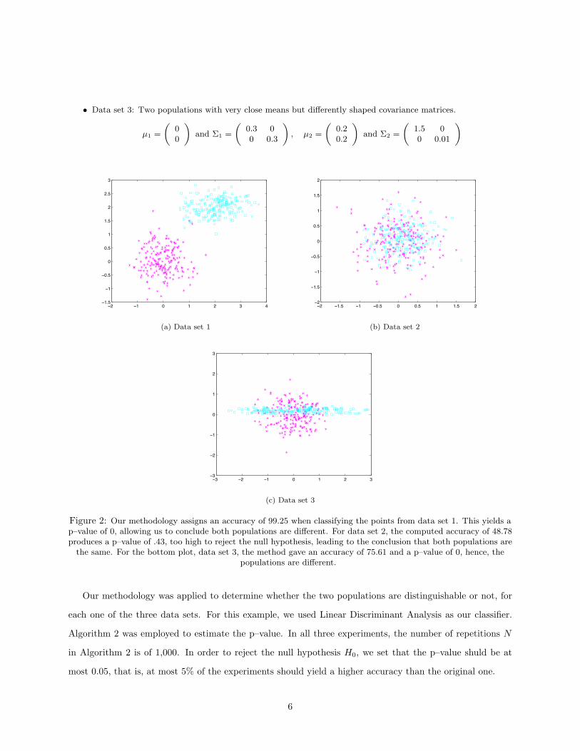
• Data set 3: Two populations with very close means but differently shaped covariance matrices.

µ1 =

(00

)and Σ1 =

(0.3 00 0.3

), µ2 =

(0.20.2

)and Σ2 =

(1.5 00 0.01

)

−2 −1 0 1 2 3 4−1.5

−1

−0.5

0

0.5

1

1.5

2

2.5

3

(a) Data set 1

−2 −1.5 −1 −0.5 0 0.5 1 1.5 2−2

−1.5

−1

−0.5

0

0.5

1

1.5

2

(b) Data set 2

−3 −2 −1 0 1 2 3−3

−2

−1

0

1

2

3

(c) Data set 3

Figure 2: Our methodology assigns an accuracy of 99.25 when classifying the points from data set 1. This yields ap–value of 0, allowing us to conclude both populations are different. For data set 2, the computed accuracy of 48.78produces a p–value of .43, too high to reject the null hypothesis, leading to the conclusion that both populations are

the same. For the bottom plot, data set 3, the method gave an accuracy of 75.61 and a p–value of 0, hence, thepopulations are different.

Our methodology was applied to determine whether the two populations are distinguishable or not, for

each one of the three data sets. For this example, we used Linear Discriminant Analysis as our classifier.

Algorithm 2 was employed to estimate the p–value. In all three experiments, the number of repetitions N

in Algorithm 2 is of 1,000. In order to reject the null hypothesis H0, we set that the p–value shuld be at

most 0.05, that is, at most 5% of the experiments should yield a higher accuracy than the original one.

6

Table 1: Results of synthetic data experimentData set Accuracy p-value Distinguishable?Data set 1 99.25 0 YesData set 2 48.78 0.428 NoData set 3 75.61 0 Yes

The results of this experiment are presented in Table . For the first data set, the accuracy of the classifier

trained on the original dataset using Algorithm 1 is A = 99.25. Applying Algorithm 2 produces a p–value

of 0. Hence, the null hypothesis H0 can be rejected and we conclude that the two populations are different.

For the second data set, Algorithm 1 gives an accuracy of A = 48.78. Algorithm 2 outputs a p–value of 0.428

– which is too large to be rejected. Hence, we cannot reject the null hypothesis H0 and cannot distinguish

between both populations.

In the third case, the accuracy of the classifier is 75.61 and the p–value is 0. This corresponds to what one

would expect: even though the means of these two classes are close, their shape is very different, hence, one

would like the test to find them different.

Notice how in data set 1 and 3, the p–value estimated by Algorithm 2 is 0. This means, out of the 1,000

experiments, not a single one yielded a higher accuracy than the original accuracy A. However, the true

p–value might not be 0, but a number very close to 0. A possible way for estimating the p–value would be

by fitting a probability density function ρ(x) to the accuracies A∗ computed in Algorithm 2. After this is

done, the p–value becomes

p–value =∫ ∞

A

ρ(x)dx

This process, however, is beyond the scope of this article.

In the following sections, the methodology developed in this article is applied to hit detection of Drosophila.

Results

In this section, we describe the application of our algorithm to identifying Drosophila larval behavioral

“mutants”. We describe the biological experiment and the data set it yielded, as well as present and discuss

the results produced by our methodology.

7

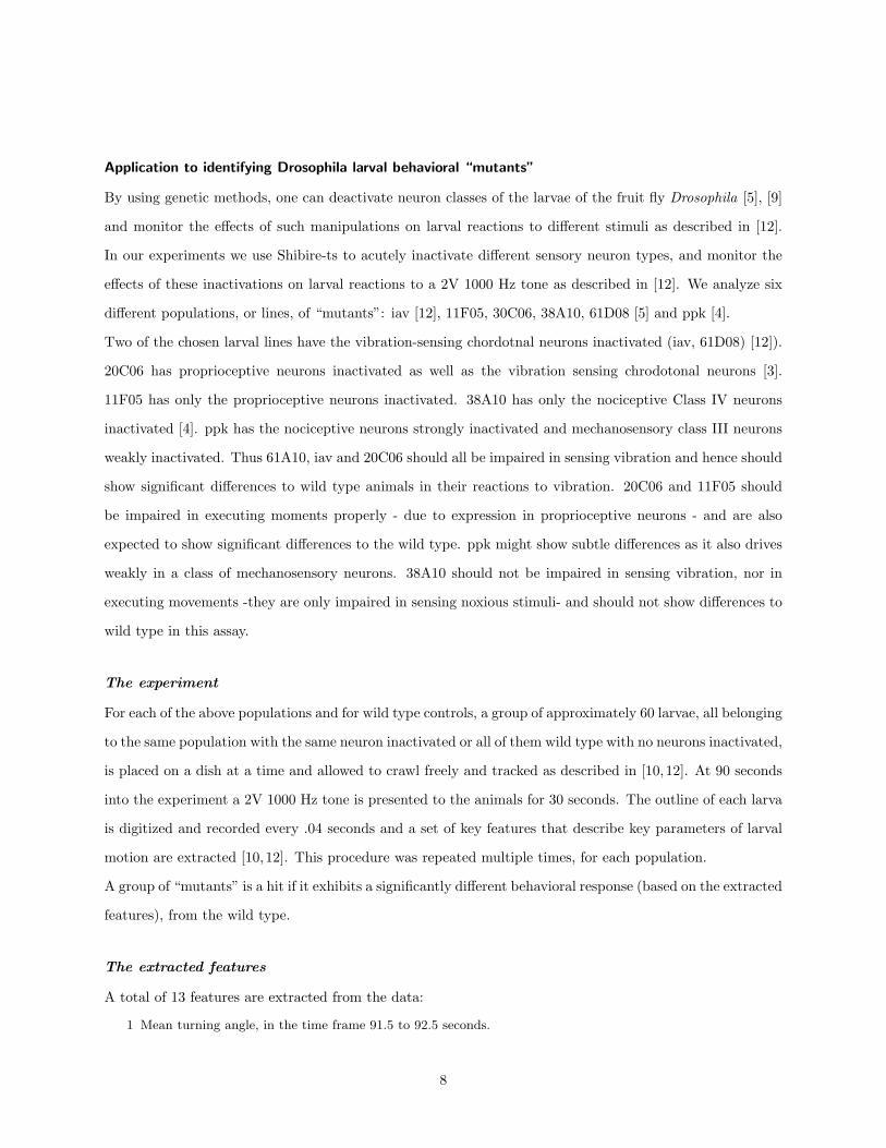
Application to identifying Drosophila larval behavioral “mutants”

By using genetic methods, one can deactivate neuron classes of the larvae of the fruit fly Drosophila [5], [9]

and monitor the effects of such manipulations on larval reactions to different stimuli as described in [12].

In our experiments we use Shibire-ts to acutely inactivate different sensory neuron types, and monitor the

effects of these inactivations on larval reactions to a 2V 1000 Hz tone as described in [12]. We analyze six

different populations, or lines, of “mutants”: iav [12], 11F05, 30C06, 38A10, 61D08 [5] and ppk [4].

Two of the chosen larval lines have the vibration-sensing chordotnal neurons inactivated (iav, 61D08) [12]).

20C06 has proprioceptive neurons inactivated as well as the vibration sensing chrodotonal neurons [3].

11F05 has only the proprioceptive neurons inactivated. 38A10 has only the nociceptive Class IV neurons

inactivated [4]. ppk has the nociceptive neurons strongly inactivated and mechanosensory class III neurons

weakly inactivated. Thus 61A10, iav and 20C06 should all be impaired in sensing vibration and hence should

show significant differences to wild type animals in their reactions to vibration. 20C06 and 11F05 should

be impaired in executing moments properly - due to expression in proprioceptive neurons - and are also

expected to show significant differences to the wild type. ppk might show subtle differences as it also drives

weakly in a class of mechanosensory neurons. 38A10 should not be impaired in sensing vibration, nor in

executing movements -they are only impaired in sensing noxious stimuli- and should not show differences to

wild type in this assay.

The experiment

For each of the above populations and for wild type controls, a group of approximately 60 larvae, all belonging

to the same population with the same neuron inactivated or all of them wild type with no neurons inactivated,

is placed on a dish at a time and allowed to crawl freely and tracked as described in [10,12]. At 90 seconds

into the experiment a 2V 1000 Hz tone is presented to the animals for 30 seconds. The outline of each larva

is digitized and recorded every .04 seconds and a set of key features that describe key parameters of larval

motion are extracted [10,12]. This procedure was repeated multiple times, for each population.

A group of “mutants” is a hit if it exhibits a significantly different behavioral response (based on the extracted

features), from the wild type.

The extracted features

A total of 13 features are extracted from the data:

1 Mean turning angle, in the time frame 91.5 to 92.5 seconds.

8

2 Mean forward-backward crawling bias, in the time frame 90.5 to 91.5 seconds.

3 Mean crawling direction, in the time frame 90.5 to 91 seconds.

4 Mean crawling speed, in the time frame 100 to 101 seconds.

5 Frequency of crawling strides, in the time frame 110 to 120 seconds.

6 Maximum speed of individual crawling strides, in the time frame 110 to 120 seconds.

7 A binary variable indicating whether the animal presents one or more turns in the time frame 91 to 96 seconds.

• If the animal presents one or more head turns in the time frame 91 to 96 seconds:

8 Mean amplitude of head turns.

9 Mean duration of head turns.

10 Frequency of head turns, that is, number of events divided by the length of the time interval.

• If the animal presents one or more head retractions in the time frame 90 to 95 seconds:

11 Mean amplitude of head retractions.

12 Mean duration of head retractions.

13 Frequency of head retractions, that is, number of events divided by the length of the time interval.

The first seven features are provided for every animal. If it turns in the specified time frame, we have three

more features. Similarly, if the animal retracts its head, we have three extra features. Not all animals present

head turns or head retractions, especially head retractions. There are some “mutant” populations of larvae

where only two or three animals present head retractions. However, a reasonable number of them do turn.

In our analysis, we will ignore the head retraction feature, and include the turn feature.

Data set selection

There are two kinds of defects “mutants” can exhibit with regard to a specific action, for example, a turn:

One is, the animals simply do not present the action or present it with a frequency different from the wild

type. The other, they do the action with the same frequency as wild type animals, but the action itself is

abnormal in some way, for example in its duration or amplitude. Hence, we conduct our study using two

different subsets of the “mutant ” class Cm:

• Use all the animals in the mutant class, and the first seven features measured in all animals. We shall

call this set Cm, and nm will denote the number of animals in this class.

• Select only the animals that perform turns ,and include the features that describe the chacracteristics

of the turn (features 8 - 10). We will refer to this set as Cm,t, and the number of animals in this set

will be nm,t. For these animals, the binary feature that indicates turning (7) will always be 1, hence

we discard it.

9

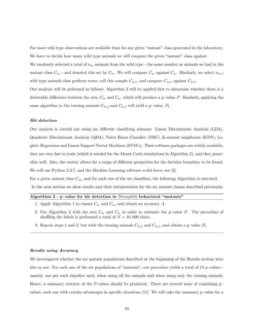
Far more wild type observations are available than for any given “mutant” class generated in the laboratory.

We have to decide how many wild type animals we will compare the given “mutant” class against.

We randomly selected a total of nm animals from the wild type - the same number as animals we had in the

mutant class Cm - and denoted this set by Cw. We will compare Cm against Cw. SImilarly, we select nm,t

wild type animals that perform turns, call this sample Cw,t, and compare Cm,t against Cw,t.

Our analysis will be peformed as follows: Algorithm 2 will be applied first to determine whether there is a

detectable difference between the sets, Cm and Cw, which will produce a p–value P . Similarly, applying the

same algorithm to the turning animals Cm,t and Cw,t will yield a p–value, Pt.

Hit detection

Our analysis is carried out using six different classifying schemes: Linear Discriminate Analysis (LDA),

Quadratic Discriminant Analysis (QDA), Naive Bayes Classifier (NBC), K-nearest neighboors (KNN), Lo-

gistic Regression and Linear Support Vector Machines (SVM’s). Their software packages are widely available,

they are very fast to train (which is needed for the Monte Carlo simulations in Algorithm 2), and they gener-

alize well. Also, the variety allows for a range of different geometries for the decision boundary to be found.

We will use Python 2.3.7, and the Machine Learning software scikit-learn, see [6].

For a given mutant class Cm, and for each one of the six classifiers, the following Algorithm is executed.

In the next section we show results and their interpretation for the six mutant classes described previously.

Algorithm 3 - p–value for hit detection in Drosophila behavioral “mutants”

1. Apply Algorithm 1 to classes Cm and Cw, and obtain an accuracy A.

2. Use Algorithm 2 with the sets Cm and Cw in order to estimate the p–value P . The procedure ofshuffling the labels is performed a total of N = 10, 000 times.

3. Repeat steps 1 and 2, but with the turning animals Cm,t and Cw,t, and obtain a p–value Pt.

Results using Accuracy

We investigated whether the six mutant populations described at the beginning of the Results section were

hits or not. For each one of the six populations of “mutants”, our procedure yields a total of 12 p–values -

namely, one per each classifier used, when using all the animals and when using only the turning animals.

Hence, a summary statistic of the P-values should be produced. There are several ways of combining p–

values, each one with certain advantages in specific situations [11]. We will take the summary p–value for a

10

Table 2: Summary of results for the 6 populations studied, using Accuracy.Population Turn: Yes/No p–val: Min (Max)

EXT –iav-GAL4 233 / 145 0.000 (0.019)GMR – 11F05 248 / 193 0.001 (0.149)GMR – 20C06 106 / 356 0.000 (0.002)GMR – 38A10 168 / 174 0.233 (0.431)GMR – 61D08 165 / 210 0.001 (0.078)

MZZ – ppk1d9GAL4 292 / 222 0.029 (0.299)

given mutant class to be the minimum value among classifiers. In order to reject the null hypothesis H0 for

a specific mutant class, we set that at least one of the p–values computed, either P or Pt, should be at most

0.01. That is, for at least one classifier and one analysis, either using all the animals or only the ones that

turn, at most 1% of the experiments can yield a higher accuracy A∗ than our original median accuracy A.

A summary of the results for all six populations is presented in Table 2.

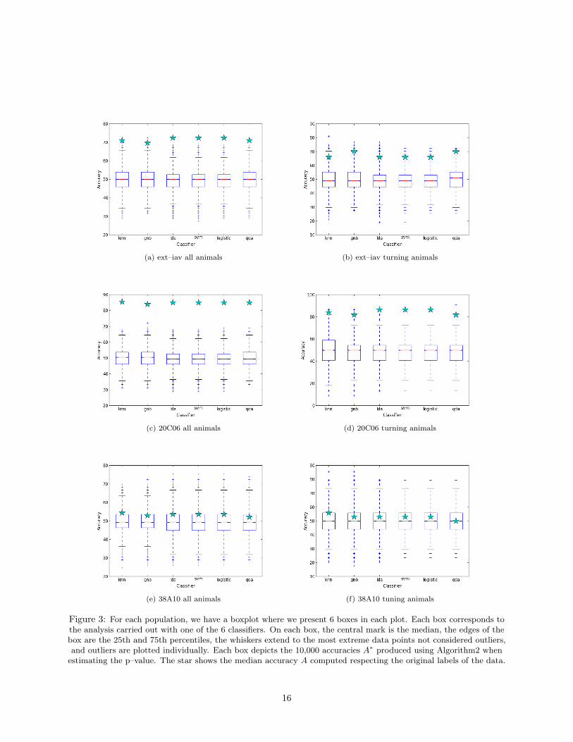
For the larval lines iav, 20C06 and 38A10, we present the following results:

• A table with the median accuracies A and At, for each one of the six classifiers trained using all animals

and only turning animals, and the p–values associated with them, P and Pt, obtained with Algorithm

2.

• Two box plots, one for the analysis using all the animals and one for the ones that turn. We present six

boxes in each plot, one per classifier used. Each box depicts the 10,000 accuracies A∗ produced using

Algorithm 2 when estimating the p–value, as well as the median accuracy A computed respecting the

orignal labels of the data.

The corresponding tables and boxplots for 11F05, 61D08 and ppk are in the supplement file.

In four cases (iav, 11F05, 20C06 and 61D08), our procedure yielded a small enough p–value to be able to

conclude that using the measurements at hand, and with the classifiers chosen for this study, we can say

that these four populations are distinguishable from the wild type, that is, that they are a hit.

For the remaining populations (38A10 and ppk), our methodology could not conclude that the difference

between it and the wild type was significant.

Results using Mean Squared Error

Certain classifiers output not only to which class a sample belongs to, but also the probability that it belongs

to that class. Let Pi(x) denote the probability of x belonging to Ci, the i-th class. P will be a distribution,

11

Table 3: Population EXT –iav-GAL4Classifier A P At Pt

knn 71.052 0.000 65.957 0.019

gnb 69.737 0.000 70.213 0.004

lda 72.368 0.000 65.957 0.017

svm 72.368 0.000 65.957 0.016

logistic 72.368 0.000 65.957 0.016

qda 71.052 0.000 70.213 0.004

Table 4: Population GMR – 20C06Classifier A P At Pt

knn 85.483 0.000 84.091 0.000

gnb 83.871 0.000 81.818 0.002

lda 84.946 0.000 86.364 0.000

svm 84.946 0.000 86.364 0.000

logistic 84.946 0.000 86.364 0.000

qda 84.946 0.000 81.818 0.001

assigining to each sample the probability of it belonging to each class. In this situation, there are different

ways one could measure the distance between these estimated assignments P and the true assignments of

the data, that is, their known memberships. We will consider the mean squared error (MSE), given by:

MSE =1N

∑i

∑x∈Ci

(1− Pi(x))2

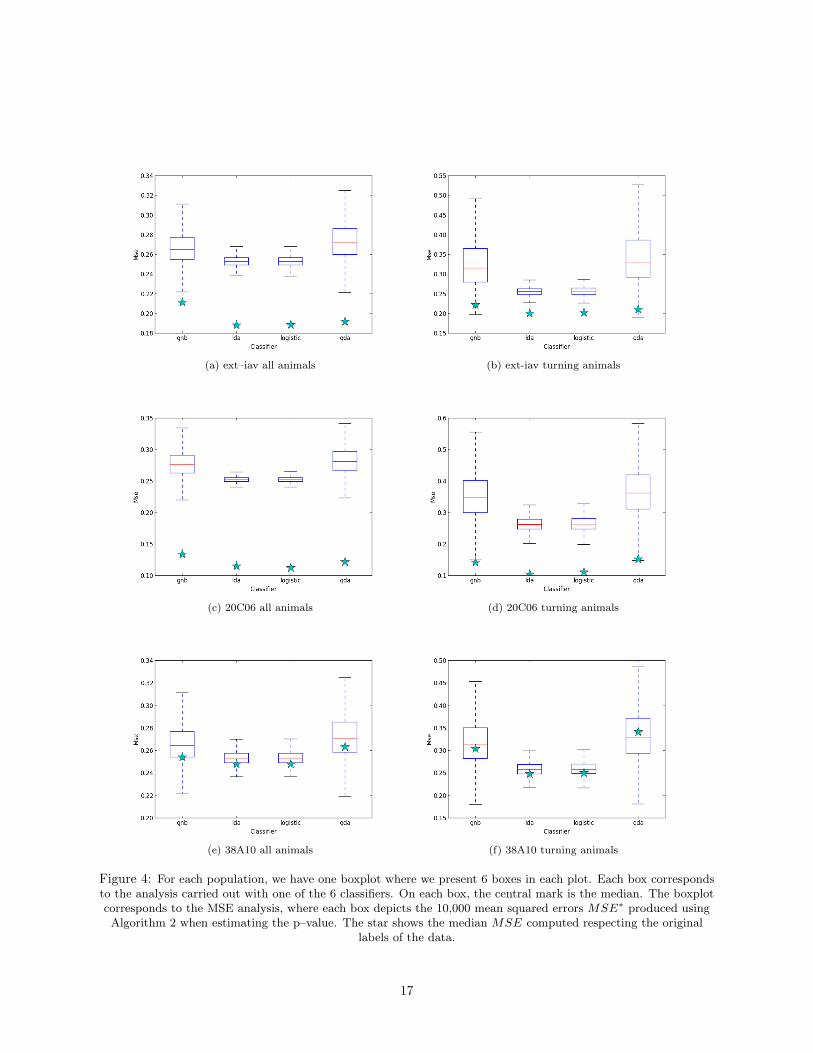
We present a study, analogous to that of the previous sections, for this measurement. The classifiers used

will be Linear and Quadratic Discriminant Analysis, Logistic regression and Gaussian Naive Bayes. Using

Algorithm 1, we can estimate a mean squared error MSE. Afterwards, Algorithm 2 is carried out in order

to estimate the probability of having observed a mean squared error MSE∗, using shuffled labels, of at most

MSE - the one computed respecting the true labels. A summary of the results is shown in Table 6. We also

show the tables and box plots for three populations. The remaining results can be found in the Additional

File 1.

We notice that our methodology using MSE as the measurement for the performance of the classifiers

Table 5: Population GMR – 38A10Classifier A P At Pt

knn 54.348 0.233 55.882 0.297

gnb 52.899 0.289 52.941 0.431

lda 53.623 0.279 52.941 0.392

svm 53.623 0.279 52.941 0.388

logistic 53.623 0.279 52.941 0.391

qda 52.174 0.386 50.000 0.562

12

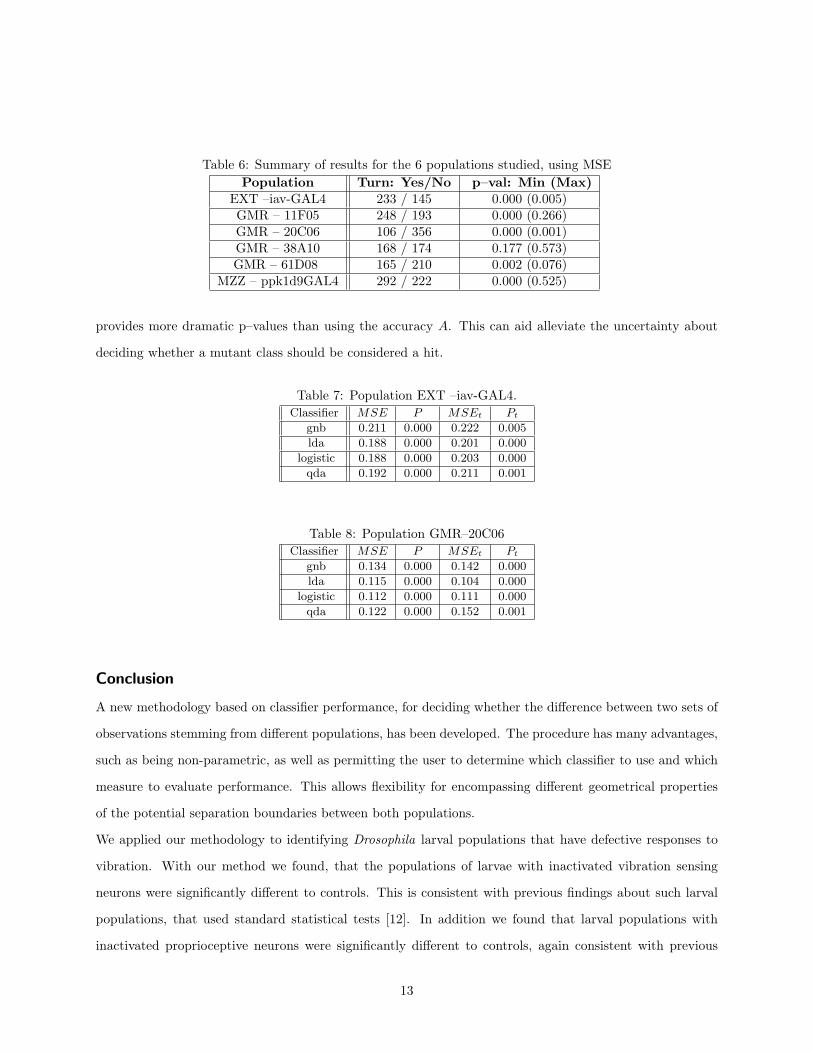
Table 6: Summary of results for the 6 populations studied, using MSEPopulation Turn: Yes/No p–val: Min (Max)

EXT –iav-GAL4 233 / 145 0.000 (0.005)GMR – 11F05 248 / 193 0.000 (0.266)GMR – 20C06 106 / 356 0.000 (0.001)GMR – 38A10 168 / 174 0.177 (0.573)GMR – 61D08 165 / 210 0.002 (0.076)

MZZ – ppk1d9GAL4 292 / 222 0.000 (0.525)

provides more dramatic p–values than using the accuracy A. This can aid alleviate the uncertainty about

deciding whether a mutant class should be considered a hit.

Table 7: Population EXT –iav-GAL4.Classifier MSE P MSEt Pt

gnb 0.211 0.000 0.222 0.005

lda 0.188 0.000 0.201 0.000

logistic 0.188 0.000 0.203 0.000

qda 0.192 0.000 0.211 0.001

Table 8: Population GMR–20C06Classifier MSE P MSEt Pt

gnb 0.134 0.000 0.142 0.000

lda 0.115 0.000 0.104 0.000

logistic 0.112 0.000 0.111 0.000

qda 0.122 0.000 0.152 0.001

Conclusion

A new methodology based on classifier performance, for deciding whether the difference between two sets of

observations stemming from different populations, has been developed. The procedure has many advantages,

such as being non-parametric, as well as permitting the user to determine which classifier to use and which

measure to evaluate performance. This allows flexibility for encompassing different geometrical properties

of the potential separation boundaries between both populations.

We applied our methodology to identifying Drosophila larval populations that have defective responses to

vibration. With our method we found, that the populations of larvae with inactivated vibration sensing

neurons were significantly different to controls. This is consistent with previous findings about such larval

populations, that used standard statistical tests [12]. In addition we found that larval populations with

inactivated proprioceptive neurons were significantly different to controls, again consistent with previous

13

Table 9: Population GMR – 38A10.Classifier MSE P MSEt Pt

gnb 0.254 0.249 0.304 0.414

lda 0.248 0.177 0.248 0.250

logistic 0.248 0.177 0.250 0.291

qda 0.263 0.345 0.341 0.573

findings. We also found that larval populations with inactivated nociceptive neurons were not significantly

different to controls. The ppk line that has weakly inactivated class III mechanosensory neurons as well as

nociceptive neurons was found to be slightly significantly different, albeit not as strongly significant as the

61D08, iav or 20C06. We therefore show that with our approach we can confirm previous findings.

We hope this methodology will shed some light, either detecting differences between populations too subtle

to be notice by traditional hypothesis testing methods, or by giving us a dependable way of declaring there

is indeed no significant difference between two sets of observations.

Author’s contributions

TO and MZ concieved the biological study. TO and MZ designed and conducted the experiments. TO

and MZ extracted the features and provided the data set, carried out initial analyses and selected the

six populations of larvae of interest. MZ, ET and RSB discussed the idea of developing a new means of

hypothesis testing. RSB conceived the algorithm for hypothesis testing and implemented it numerically, in

the synthetic and biological data. ET helped further develop the algorithm and analize the results. MZ,

ET and RSB interpreted the final results, with MZ providing the biological explanation. RSB wrote the

manuscript, and MZ and ET revised and edited it. All authors have read and approved this manuscript.

Acknowledgements

We would like to thank C. Montell (John Hopkins U), for providing the iav-GAL4, D. Tracey (Duke Uni-

versity) for providing ppk1.9 GAL4, and M. Tygert (New York University) for many helpful discussions.

We would like to thank M. Mercer and K. Hibbard for fly crossing and members of Janelia’s Fly Core for

stock maintenance. M. Zlatic and T. Oyama were supported by the Howard Hughes Medical Institute. R.

Salas-Boni was supported by an NYU MacCracken Fellowship. E. Tabak was supported by NSF grants

DMS-0908077 and DMS-1211298.

14

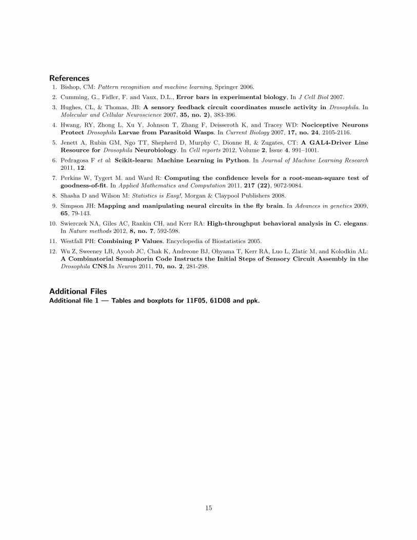
References1. Bishop, CM: Pattern recognition and machine learning, Springer 2006.

2. Cumming, G., Fidler, F. and Vaux, D.L., Error bars in experimental biology, In J Cell Biol 2007.

3. Hughes, CL, & Thomas, JB: A sensory feedback circuit coordinates muscle activity in Drosophila. InMolecular and Cellular Neuroscience 2007, 35, no. 2), 383-396.

4. Hwang, RY, Zhong L, Xu Y, Johnson T, Zhang F, Deisseroth K, and Tracey WD: Nociceptive NeuronsProtect Drosophila Larvae from Parasitoid Wasps. In Current Biology 2007, 17, no. 24, 2105-2116.

5. Jenett A, Rubin GM, Ngo TT, Shepherd D, Murphy C, Dionne H, & Zugates, CT: A GAL4-Driver LineResource for Drosophila Neurobiology. In Cell reports 2012, Volume 2, Issue 4, 991–1001.

6. Pedragosa F et al: Scikit-learn: Machine Learning in Python. In Journal of Machine Learning Research2011, 12.

7. Perkins W, Tygert M. and Ward R: Computing the confidence levels for a root-mean-square test ofgoodness-of-fit. In Applied Mathematics and Computation 2011, 217 (22), 9072-9084.

8. Shasha D and Wilson M: Statistics is Easy!, Morgan & Claypool Publishers 2008.

9. Simpson JH: Mapping and manipulating neural circuits in the fly brain. In Advances in genetics 2009,65, 79-143.

10. Swierczek NA, Giles AC, Rankin CH, and Kerr RA: High-throughput behavioral analysis in C. elegans.In Nature methods 2012, 8, no. 7, 592-598.

11. Westfall PH: Combining P Values. Encyclopedia of Biostatistics 2005.

12. Wu Z, Sweeney LB, Ayoob JC, Chak K, Andreone BJ, Ohyama T, Kerr RA, Luo L, Zlatic M, and Kolodkin AL:A Combinatorial Semaphorin Code Instructs the Initial Steps of Sensory Circuit Assembly in theDrosophila CNS.In Neuron 2011, 70, no. 2, 281-298.

Additional FilesAdditional file 1 — Tables and boxplots for 11F05, 61D08 and ppk.

15

(a) ext–iav all animals (b) ext–iav turning animals

(c) 20C06 all animals (d) 20C06 turning animals

(e) 38A10 all animals (f) 38A10 tuning animals

Figure 3: For each population, we have a boxplot where we present 6 boxes in each plot. Each box corresponds tothe analysis carried out with one of the 6 classifiers. On each box, the central mark is the median, the edges of thebox are the 25th and 75th percentiles, the whiskers extend to the most extreme data points not considered outliers,and outliers are plotted individually. Each box depicts the 10,000 accuracies A∗ produced using Algorithm2 when

estimating the p–value. The star shows the median accuracy A computed respecting the original labels of the data.

16

(a) ext–iav all animals (b) ext-iav turning animals

(c) 20C06 all animals (d) 20C06 turning animals

(e) 38A10 all animals (f) 38A10 turning animals

Figure 4: For each population, we have one boxplot where we present 6 boxes in each plot. Each box correspondsto the analysis carried out with one of the 6 classifiers. On each box, the central mark is the median. The boxplotcorresponds to the MSE analysis, where each box depicts the 10,000 mean squared errors MSE∗ produced using

Algorithm 2 when estimating the p–value. The star shows the median MSE computed respecting the originallabels of the data.

17