Multivariate Time-Series Analysis -...
89
Multivariate Time-Series Analysis Carlo Favero 2013/2014 Favero () Multivariate Time-Series Analysis 2013/2014 1 / 89
-
Upload
nguyenphuc -
Category
Documents
-
view
245 -
download
0
Transcript of Multivariate Time-Series Analysis -...

Multivariate Time-Series Analysis
Carlo Favero
2013/2014
Favero () Multivariate Time-Series Analysis 2013/2014 1 / 89

Spurious Regressions
To give an intuition of the importance of non-stationarity in time-seriesand to illustrate the problems related to non-stationarity, consider theresults of two regressions reported in the Table , obtained by relatingthe logarithm of UK stock prices to the log of US dividends and the logof UK dividends.
Favero () Multivariate Time-Series Analysis 2013/2014 2 / 89

Understanding spurious regressions
Favero () Multivariate Time-Series Analysis 2013/2014 3 / 89

Understanding spurious regressions
LDUS and LPUK can both be approximated by random walk models:
LDUSt = a0 + LDUSt�1 + ε1t,LPUKt = b0 + LPUKt�1 + ε2t,
ε1t � n.i.d.�
0, σ2ε1
�,
ε2t � n.i.d.�
0, σ2ε2
�.
As we already know, recursive substitution yields:
LDUSt = LDUS0 + a0t+t�1
∑i=0
ε1t�i,
LPUKt = LPUK0 + b0t+t�1
∑i=0
ε2t�i.
Favero () Multivariate Time-Series Analysis 2013/2014 4 / 89

Understanding Spurios Regressions
When the following model is estimated:
LPUKt = bα+ bβLDUSt + bεt,
the coefficient bβ is significant as both series have a deterministic trend.However, to have a non-spurious relation, we require that theregression also removes the stochastic trend from the dependentvariables, leaving stationary residuals.
Favero () Multivariate Time-Series Analysis 2013/2014 5 / 89

Clicker
Insert Clicker 1 here
Favero () Multivariate Time-Series Analysis 2013/2014 6 / 89
Spurious Regressions
The Durbin�Watson statistic, originally designed to test for thepresence of first-order autocorrelation in the residuals, can bere-calibrated to test for stationarity:
DW =
T∑
i=2(bεt � bεt�1)
2
T∑
i=2bε2
t
' 2 (1� bρ) ,
where bρ is the OLS coefficient from the regression of bεt on bεt�1. Thetest was originally tabulated to test the hypothesis H0: ρ = 0; however,critical values for the null of non-stationarity H0: ρ = 1 have beenprovided by Sargan and Bhargava(1983).
Favero () Multivariate Time-Series Analysis 2013/2014 7 / 89

Dynamic Models
Favero () Multivariate Time-Series Analysis 2013/2014 8 / 89

Why can a dynamic model solve the spuriousregression problem ?
The log of stock prices and the log of dividends are trendingvariables, and removing a deterministic trend from them does notdeliver stationary time-series.However. The dynamic dividend growth model is built on thehypothesis that the log of the dividend price is stationary, thismeans that, while the log of dividends and the log of prices arenon stationary, there exists a linear combination of them thatbecomes stationary.In this case we say that the two series are cointegrated with acointegrating vector (1,-1)In general, we say that two non-stationary variables integrated oforder d are cointegrated of order b, if there exists a linearcombination of them which is integrated of order d� b.
Favero () Multivariate Time-Series Analysis 2013/2014 9 / 89

Vector AutoRegressive Models
Let us consider the simplest possible multivariate model, i.e. thebivariate model and let us consider the case of the two specificvariables to our interest, lpt, the log of stock prices and ldt, the log ofdividends. We represent the dynamic process as follows:
lpt = a0 + a1lpt�1 + a2ldt�1 + ε1t.ldt = b0 + ldt�1 + ε2t.
Favero () Multivariate Time-Series Analysis 2013/2014 10 / 89
Vector Autoregressive Models
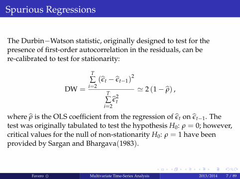
Note that system is a multivariate generalization of the univariateautoregressive process than can be re-written as :
Yt = A0 +A1Yt�1 + εt
Yt =
�lptldt
�, εt =
�ε1tε2t
�A0 =
�a0b0
�, A1 =
�a1 a20 1
�The model is therefore naturally called a VAR (Vector AutoregressiveProcess).
Favero () Multivariate Time-Series Analysis 2013/2014 11 / 89

Cointegrated VARs
Cointegration has interesting implications for VAR representation.Consider the following re-parameterization of our VAR :
∆lpt = a0 + α (lpt�1 � β1ldt�1) + ε1t,∆ldt = b0 + ε2t.
α = (1� a1) , β1 =a2
1� a1.
The estimated dynamic model includes both first differences andlevels. The presence of the level variables generates a long-runsolution, derived by setting all first differences either to zero (steadystate with no deterministic trend) or a constant (steady state). α plays acrucial role and determines the dynamic properties of the system. β1defines the long-run relation between lp and ld.
Favero () Multivariate Time-Series Analysis 2013/2014 12 / 89
Cointegrated VARs
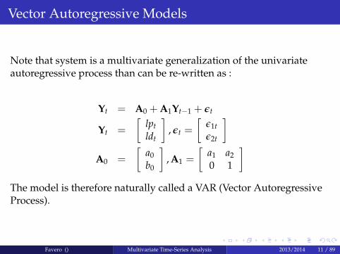
we can interpret β1ld as the long-run equilibrium level lp� for thelog of prices.When α < 0, prices increase at time t whenever lpt�1 < lp�t�1, anddecreases whenever lpt�1 > lp�t�1. The system equilibrates in thepresence of disequilibrium (i.e. a discrepancy between lp and lp�).Such error correction features guarantee that (lpt � lp�t ) isstationary. This in fact defines cointegration.
Favero () Multivariate Time-Series Analysis 2013/2014 13 / 89

Cointegrated VARs
Cointegration implies an ECM representation, which allows us tore-write a model in levels, involving non-stationary time-series, asa model involving only stationary variables. Such variables arestationary either because they are the first differences ofnon-stationary variables or because they are stationary linearcombinations of non-stationary variables (cointegrating vectors).We can reinterpret in terms of cointegration between prices anddividends the results of the predictive regressions of stock marketreturns on the dividend price ratio.
Favero () Multivariate Time-Series Analysis 2013/2014 14 / 89

Clicker
Insert Clicker 2 here
Favero () Multivariate Time-Series Analysis 2013/2014 15 / 89

The properties of CVARs
To show the properties of the model, we first generate samples for thetwo innovation processes; then we generate artificial data for pricesand dividends by constructing the above model and solving itdynamically. We do so for a sample of 200 observations. The simulatedseries in levels (lptand ldt) are plotted in the following Figure:
Favero () Multivariate Time-Series Analysis 2013/2014 16 / 89

The properties of CVARs
The parameter α in the ECM specification determines the speed ofadjustment in the presence of disequilibrium. To illustrate the role ofthis parameter we report the two series (lpt-ldt) generated by takingthe same innovations for the sample 1:200. The process (??) is used togenerate the first time-series of disequilibria (lpt-ldt), while the secondtime-series (lpt-ld1
t ) is generated by keeping all the parametersunchanged with the exception of α, which is changed from 0.15 to 0.8.The resulting observations for disequilibria are reported in thefollowing Figure
Favero () Multivariate Time-Series Analysis 2013/2014 17 / 89

Static Regressions and Dynamic Models
Given the following DGP:
yt = a1yt�1 + a2xt + a3xt�1 + u1t,xt = b1xt�1 + u2t,�
u1tu2t
�� N.I.D.
��00
�,�
σ11 00 σ22
��,
a static model is estimated by OLS:
yt = γxt + εt,bγ =∑ xtyt
∑ x2t
.
Favero () Multivariate Time-Series Analysis 2013/2014 18 / 89

Static Regressions and Dynamic Models
p lim bγ = p lim�
a1∑ xtyt�1/T
∑ x2t /T
+ a2 + a3∑ xtxt�1/T
∑ x2t /T
+∑ xtu1t/T
∑ x2t /T
�.
Under the hypothesis (jb1j < 1), we can substitute for xt in terms ofxt�1 and u2t and apply Slutsky’s and Cramer’s theorems to derive thefollowing result:
p lim bγ =a2 + a3b1
1� a1b1,
a2 � p lim bγ � a2 + a3
1� a1.
Favero () Multivariate Time-Series Analysis 2013/2014 19 / 89

Cointegration and Forecasting Stock Market returns atdifferent horizons
Favero () Multivariate Time-Series Analysis 2013/2014 20 / 89

Cointegration and Forecasting Stock Market returns atdifferent horizons
The pattern of significance in the regressions might depend on thefact that a rolling summation of series integrated of order zerobehaves asymptotically as a series integrated of order one and,whenever the regressor is persistent, the well-know occurrence ofspurious regression between I(1) variables emerges.Having established that estimation and testing using long-horizonvariables cannot be carried out using the usual regressionmethods, Valkanov(2003) proposes propose a rescaled t-statistic,t/p
T, for testing long-horizon regressions.The asymptotic distribution of this statistic, although non-normal,is easy to simulate and the results are applicable to a general classof long-horizon regressions.
Favero () Multivariate Time-Series Analysis 2013/2014 21 / 89

Valkanov’s test
consider the following DGP:
r1t+1 = α+ βlpdt + ε1t,
(1+ φL) lpdt = µ+ ε2t.
φ = 1+cT�
ε1tε2t
�� N.I.D.
��00
�,�
σ11 σ12σ12 σ22
��
Favero () Multivariate Time-Series Analysis 2013/2014 22 / 89

Valkanov’s test
The long-horizon variables are
Zkt = rk
t+1 =k
∑j=1
r1t+1
The regression at different horizon is run by projecting Zkt on lpdt.The
simulation of the relevant distribution requires an estimate of thenuisance parameter c.
Favero () Multivariate Time-Series Analysis 2013/2014 23 / 89

Valkanov’s test
r1t+1 = ρ0 + ρlpdt+1 + ∆dt+1 � lpdt
assuming that the log-dividends follows an autoregressive process:
lpdt+1 = φlpdt + ut.
by substituting we have that
r1t+1 = ρ0 � β1lpdt + εt+1
εt+1 = ∆dt+1 + ut.β1 = (1� ρφ)
Favero () Multivariate Time-Series Analysis 2013/2014 24 / 89

Valkanov’s test
The k-period horizon return can then be written as follows:
rkt+1 � k̃� βkxt + ε̃t+1
βk =
"(1� ρφ)
k�1
∑i=0:
φi
#
Now, we can write
βk =
�(1� ρφ)
1� φk
1� φ
�
Favero () Multivariate Time-Series Analysis 2013/2014 25 / 89

Valkanov’s test
Now, consider the case in which ρ is close to 1, and remember that
φ = 1+cT
and we can express k in terms of the total length of the
available sample as,k = bλTc, from which T � kλ
. Then:
βk = 1��
1+cT
�k= 1�
�1+
cλ
k
�k
limk�!∞
�1+
cλ
k
�k
= ecλ
limk�!∞
βk = limT�!∞
βbλTc = 1� ecλ
Since we can estimate βk consistently, we can also find a consistentestimate of c by using the transformation:
cCONSISTENT =1λ
log (1� βk)
Favero () Multivariate Time-Series Analysis 2013/2014 26 / 89

Clicker
Insert Clicker 3 here
Favero () Multivariate Time-Series Analysis 2013/2014 27 / 89

Cointegration with Multiple Cointegrating Vectors
Consider the case of an econometrician who uses cointegrationtechniques to investigate simultaneously yields on long-term bonds,short term bonds and the stock market.
The dynamic dividend growth implies (lp� ld) is stationarysimilarly for bond returns we have that the term spread(St = Rt � rt) is stationary.
Favero () Multivariate Time-Series Analysis 2013/2014 28 / 89

Cointegration with Multiple Cointegrating Vectors
lpt = a0 + a1lpt�1 + a2ldt�1 +
+a3Rt�1,T + a4rt�1 + ε1t,
This statistical model fits the data well. As it is found that a1 < 1.Themodel is reparameterised as follows:
∆lpt = a0 + (a1 � 1)�lpt�1 � (lp)�t�1
�+ ut
(lp)�t�1 =a2
1� a1ldt�1 +
a3
1� a1Rt�1,T +
a4
1� a1rt�1.
Favero () Multivariate Time-Series Analysis 2013/2014 29 / 89

Cointegration with Multiple Cointegrating Vectors
As a matter of fact the variables considered might admit twocointegrating relationship, one capturing the stock market dynamicsand the other the bond market dynamics:
∆lpt = a0 + (a1 � 1) [lpt�1 � ldt�1] + a3 (Rt�1,T � rt�1) + ut
we have an identification problem
Favero () Multivariate Time-Series Analysis 2013/2014 30 / 89

Clicker
Insert Clicker 4 here
Favero () Multivariate Time-Series Analysis 2013/2014 31 / 89

The Johansen Procedure
Consider the multivariate generalization of the single-equationdynamic model discussed above, i.e. a vector autoregressive model(VAR) for the vector of, possibly non-stationary, m-variables y:
yt = A1yt�1 +A2yt�2 + ...+Anyt�n + ut.
subtract yt�1 from both sides of the VAR to obtain:
∆yt = (A1 � I) yt�1 +A2yt�2 + ...+Anyt�n + ut.
Subtract (A1 � I) yt�2 from both sides:
∆yt = (A1 � I)∆yt�1 + (A1 +A2 � I) yt�2 + ...+Anyt�n + ut.
Favero () Multivariate Time-Series Analysis 2013/2014 32 / 89

The Johansen Procedure
By repeating this procedure until n� 1, we end up with the followingspecification:
∆yt = Π1∆yt�1 +Π1∆yt�2 + ...+Πyt�n + ut
=n�1
∑i=1
Πi∆yt�i +Πyt�n + ut,
where:
Πi = �
I�i
∑j=1
Aj
!,
Π = �
I�n
∑i=1
Ai
!.
Clearly the long-run properties of the system are described by theproperties of the matrix Π.
Favero () Multivariate Time-Series Analysis 2013/2014 33 / 89

The Johansen Procedure
There are three cases of interest:
1 rank (Π) = 0. The system is non-stationary, with no cointegrationbetween the variables considered. This is the only case in whichnon-stationarity is correctly removed simply by taking the firstdifferences of the variables;
2 rank (Π) = m, full. The system is stationary;3 rank (Π) = k < m. The system is non-stationary but there are k
cointegrating relationships among the considered variables. Inthis case Π = αβ0, where α is an (m� k) matrix of weights and βis an (m� k) matrix of parameters determining the cointegratingrelationships.
Favero () Multivariate Time-Series Analysis 2013/2014 34 / 89

The Johansen Procedure
Therefore, the rank of Π is crucial in determining the number ofcointegrating vectors.
The Johansen procedure is based on the fact that the rank of amatrix equals the number of its characteristic roots that differfrom zero.Having obtained estimates for the parameters in the Π matrix, weassociate with them estimates for the m characteristic roots andwe order them as follows λ1 > λ2 > ... > λm.If the variables are not cointegrated, then the rank of Π is zero andall the characteristic roots equal zero.
In this case each of the expression ln (1� λi) equals zero, too.If, instead, the rank of Π is one, and 0 < λ1 < 1, then ln (1� λ1) isnegative and ln (1� λ2) = ln (1� λ3) = ... = ln (1� λm) = 0.
Favero () Multivariate Time-Series Analysis 2013/2014 35 / 89

The Johansen Procedure
Johansen derives a test on the number of characteristic roots that aredifferent from zero by considering the two following statistics:
λtrace (k) = �Tm
∑i=k+1
ln�
1� bλi
�,
λmax (k, k+ 1) = �T ln�
1� bλk+1
�,
where T is the number of observations used to estimate the VAR. Thefirst statistic tests the null of at most k cointegrating vectors against ageneric alternative. The test should be run in sequence starting fromthe null of at most zero cointegrating vectors up to the case of at mostm cointegrating vectors. The second statistic tests the null of at most kcointegrating vectors against the alternative of at most k+ 1cointegrating vectors.Critical values are tabulated by Johansen and they depend on thenumber of non-stationary components under the null and on thespecification of the deterministic component of the VAR.Favero () Multivariate Time-Series Analysis 2013/2014 36 / 89

An example
Consider the VAR representation of our simple dynamic model (??)for the two variables, x and y:�
ytxt
�=
�a11 a120 1
��yt�1xt�1
�+
�u1tu2t
�.
This system can be reparameterized as follows in terms of the VECMrepresentation:�
∆yt∆xt
�=
�a11 � 1 a12
0 0
��yt�1xt�1
�+
�u1tu2t
�,
from which, clearly,
Π =
�a11 � 1 a12
0 0
�, α =
�a11 � 1
0
�, β0 =
�1 � a12
1�a11
�.
Favero () Multivariate Time-Series Analysis 2013/2014 37 / 89

Cointegration in the Bond and Stock Markets
The baseline VAR can be specified as:2664lptldt
Rt,Trt
3775 = A0 +A1
2664lpt�1ldt�1
Rt�1,Trt�1
3775++2664
u1tu2tu3tu4t
3775 ,
which could then be reparameterized in VECM form:2664∆lpt∆ldt
∆Rt,T∆rt
3775 = Π0 +Π
2664lpt�1ldt�1
Rt�1,Trt�1
3775+2664
u1tu2tu3tu4t
3775 .
Favero () Multivariate Time-Series Analysis 2013/2014 38 / 89

Cointegration in the Bond and Stock Markets
Since we know that there are two cointegrating vectors, we have:
Π = αβ0,rank Π = 2,
β0 =
�1 �1 0 00 0 1 �1
�.
A possible specification for α is :
α =
2664α11 α120 00 α320 0
3775 .
With the above specification for the loadings, stock market pricesadjusts both in presence of disequilibria in the stock and the bondmarkets, long term bonds react to the spread, while short-term ratesand dividends do not respond to disequilibria.
Favero () Multivariate Time-Series Analysis 2013/2014 39 / 89

Clicker
Insert Clicker 5 here
Favero () Multivariate Time-Series Analysis 2013/2014 40 / 89

Using VAR Models
A Cointegrated VAR, after the identification of the number and shapeof cointegrating vector(s), provides a statistical model of the jointdistribution of the variables of interests:
∆yt = αβ0yt�1 + ut (1)ut s N
�0, ∑
�where yt is a vector of length N containing the modelled variables.
The reduced form specification can be adopted directly forforecasting purposes or to describe the dynamic response of thesystem to innovations to observables, such as the VAR residuals.Some further identification choice must be made if the model is tobe used for evaluating the response of economic and financialvariables to innovations to unobservables, i.e. the "structural"shocks to some of the variables included in the VAR. Impulseresponse analysis examines the effect of a typical shock, usuallyone-standard deviation, on the time path of the variables in themodel.Favero () Multivariate Time-Series Analysis 2013/2014 41 / 89

Using VAR Models
In macroeconomics, the importance of computing impulseresponses to structural shocks is related to the fact that thesolution of a Dynamic Stochastic General Equilibrium (DSGE)model can be well approximated by a VAR, and VARs havebecome the natural tool for model evaluation.
VAR models are not estimated to yield advice on the best policy butrather to provide empirical evidence on the response ofmacroeconomic variables to policy impulses in order todiscriminate between alternative theoretical models of theeconomy. It then becomes crucial to identify policy actions usingrestrictions independent from the theoretical models
In finance, the use of VAR is more related to forecasting first andsecond moments of the distributions of returns at differenthorizons. Macro-finance model concentrate on the different role ofpermanent versus transitory shocks to understand thecomovement between financial and macroeoconomic variables.
Favero () Multivariate Time-Series Analysis 2013/2014 42 / 89

Identification of VAR
Given the estimation of a VAR the problem of extracting unobservablestructural shocks υt from the observed VAR innovations ut is usuallyaddressed by positing the following relations
Aut = Bυt,υt s N (0, I)
from which we can derive the relation between thevariance-covariance matrices of ut (observed) and νt (unobserved) asfollows:
E�utu0t
�= A�1BE
�υtυ
0t�
B0A�1.
Favero () Multivariate Time-Series Analysis 2013/2014 43 / 89

Identification of VAR
Substituting population moments with sample moments we have:c∑ = bA�1BIbB0bA�1,b∑ contains n(n+ 1)/2 different elements, which is the maximumnumber of identifiable parameters in matrices A and B.
Therefore, a necessary condition for identification is that themaximum number of parameters contained in the two matricesequals n(n+ 1)/2,As usual, for such a condition also to be sufficient foridentification no equation in should be a linear combination of theother equations in the system .As for traditional models, we have the three possible cases ofunder-identification, just-identification and over-identification.The validity of over-identifying restrictions can be tested via astatistic distributed as a χ2 with a number of degrees of freedomequal to the number of over-identifying restrictions.
Favero () Multivariate Time-Series Analysis 2013/2014 44 / 89

Description of VAR models
After the identification of structural shocks of interest, the propertiesof VAR models are described using impulse response analysis,variance decomposition and historical decomposition.Given an identified and estimated estimate structural VAR
yt =p
∑i=1
Ciyt�i + ut,
Aut = Bυt,
we can re-write it as:
Ayt =p
∑i=1
Aiyt�i + Bυt,
A�1Ai = Ci
Favero () Multivariate Time-Series Analysis 2013/2014 45 / 89

Description of VAR models
which we can express in a compact way as:
[A�A (L)] yt = Bvt
A (L) =p
∑i=1
AiLi.
By inverting [A0 �A (L)] (under the assumption of invertibility of thispolynomial) we obtain the moving average representation for our VARprocess:
yt = C (L) vt,yt = C0vt +C1vt�1 + ...+Csvt�s,
C (L) = [A0 �A (L)]�1 ,C0 = A�1
0 B.
Favero () Multivariate Time-Series Analysis 2013/2014 46 / 89

Description of VAR models
To illustrate the concept of an impulse response function, we interpret thegeneric matrix Cs within the moving average representation asfollows:
Cs =∂yt+s
∂vt.
The generic element fi, jg of matrix Cs represents the impact of a shockhitting the j-th variable of the system at time t on the i-th variable ofthe system at time t+ s.
Favero () Multivariate Time-Series Analysis 2013/2014 47 / 89

Description of VAR models
Historical decomposition is obtained by using the structural MArepresentation to separate series in the components (orthogonal toeach other) attributable to the different structural shocks.Finally forecasting error variance decomposition (FEVD) is obtained from(??) by deriving the error in forecasting ys period in the future as:
(yt+s � Etyt+s) = C0vt +C1vt�1 + ...+Csvt�s
from which we can construct the variance of such forecasting error as:
Var (yt+s � Etyt+s) = C0IC00 +C1IC01 + ...+CsIC0s
from which we can compute the share of the total variance attributableto the variance of each structural shock. Note again that suchcomposition makes sense only if shocks are orthogonal to each other.
Favero () Multivariate Time-Series Analysis 2013/2014 48 / 89

Identification
In practice, identification requires the imposition of some restrictionson the parameters of A and B. This step has been historicallyimplemented in a number of different ways.
Choleski Decompositiontemporary-persistent decompositionsign restrictionsGIRF
Favero () Multivariate Time-Series Analysis 2013/2014 49 / 89

Choleski Decomposition
In the famous article which introduced VAR methodology to theprofession, Sims (1980a) proposed the following identificationstrategy, based on the Choleski decomposition of matrices:
A =
0BB@1 0 0 0a21 1 0 0. . 1 .an1 . ann�1 1
1CCA , B
0BB@b11 0 0 00 b22 0 0. . bii. .0 0 0 bnn
1CCA . (2)
This is a just-identification scheme. It corresponds to a recursiveeconomic structure, with the most endogenous variable ordered last.A generalization of Choleski is to consider contemporaneousrestrictions that do not necessarily lead to a triangular structure of A.
Favero () Multivariate Time-Series Analysis 2013/2014 50 / 89

Clicker
Insert Clicker 6 here
Favero () Multivariate Time-Series Analysis 2013/2014 51 / 89
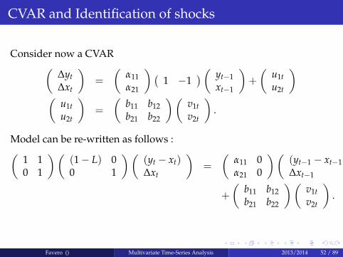
CVAR and Identification of shocks
Consider now a CVAR�∆yt∆xt
�=
�α11α21
� �1 �1
� � yt�1xt�1
�+
�u1tu2t
��
u1tu2t
�=
�b11 b12b21 b22
��v1tv2t
�.
Model can be re-written as follows :�1 10 1
��(1� L) 00 1
��(yt � xt)∆xt
�=
�α11 0α21 0
��(yt�1 � xt�1)∆xt�1
�+
�b11 b12b21 b22
��v1tv2t
�.
Favero () Multivariate Time-Series Analysis 2013/2014 52 / 89

CVAR and Identification of shocks
The cointegrating properties of the system suggest the presence of twotypes of shocks: a permanent one (related to the single common trendshared by the two variables) and a transitory one (related to thecointegrating relation).To derive long-run responses :��
1 10 1
��(1� L) 00 1
���
α11L 0α21L 0
���(yt � xt)∆xt
�=
�b11 b12b21 b22
��v1tv2t
�,
from which long-run responses are obtained by setting L = 1 and byinverting the matrix pre-multiplying variables in the stationaryrepresentation of VAR�
(yt � xt)∆xt
�=
��α11 1�α21 1
��1 � b11 b12b21 b22
��v1tv2t
�
Favero () Multivariate Time-Series Analysis 2013/2014 53 / 89

CVAR and Identification of shocks
�(yt � xt)∆xt
�=
�b11+b21α11�α21
� b12�b22α11�α21�α21b11+α11b21
α11�α21
�α21b12+α11b22α11�α21
!�v1tv2t
�.
Thus v2t can be identified as the transitory shock by imposing thefollowing restriction:
�α21b12 + α11b22 = 0
which, given knowledge of the α parameters from the cointegrationanalysis, provides the just-identifying restriction for the parameters inB. Note that, there is one case in which this identification is equivalentto the Choleski ordering, the case in which α11 = 0. Note that this isthe case in which ∆yt is weakly exogenous for the estimation of b21.
Favero () Multivariate Time-Series Analysis 2013/2014 54 / 89

Sign Restrictions
Given the VAR specification:
yt =p
∑i=1
Aiyt�i + But
Σ = BE�utu0t
�B0 = BB0
Consider the Choleski decomposition of Σ, C .The impulse response function, given the Choleski decompositioncould be written as :
yt = [I�A (L)]�1 Cut
Favero () Multivariate Time-Series Analysis 2013/2014 55 / 89

Sign Restrictions
All the possible rotation of the Choleski decomposition are obtained asfollows:
[I�A (L)]�1 CQQ0ut
QQ0 = I
The impulse response for Q0ut, is then [I�A (L)]�1 CQ.The imposition of the sign restrictions then consider Q to generate allpossible identification and then select only those that satisfy some signrestriction.
Favero () Multivariate Time-Series Analysis 2013/2014 56 / 89

GIRF
If the identification of structural shocks is not an issue of primaryinterest then Generalized Impulse Response Functions can be used todescribe the respoonse of the system to change in observable i.e. theVAR innovations.Consider again our bivariate CVAR model :
�(yt � xt)∆xt
�= A
�(yt�1 � xt�1)∆xt�1
�+ ut
ut s N�
0,�
σ211 σ12
σ12 σ222
��
Favero () Multivariate Time-Series Analysis 2013/2014 57 / 89

GIRF
from the properties of the normal distribution we have that
E (u2t j u1t) =�
σ211
��1σ12u1t
so the impulse responses can be derived as follows:
∂
�(yt+i � xt+i)∆xt + i
�∂u1t
= AiS
S =
1�
σ211��1
σ12
!
GIRF seems to be more appropriate when the primary focus of theanalysis is the description of the transmission mechanism rather thanthe structural interpretation of shocks.
Favero () Multivariate Time-Series Analysis 2013/2014 58 / 89

Cointegration and PV Models
Consider a vector yt containing two variables xt and zt cointegratedwith an equilibrium error St = xt � βzt.The Johansen representation for such system will be:
�∆xt∆zt
�= Π1
�∆xt�1∆zt�1
�+
�α11α21
� �1 �β
� � xt�1zt�1
�+
�v1tv2t
�.�
∆xt∆zt
�= Π1
�∆xt�1∆zt�1
�+
�α11α21
�St�1 +
�v1tv2t
�
Favero () Multivariate Time-Series Analysis 2013/2014 59 / 89

Cointegration and PV Models
Define a matrix M such that
M�
∆xt∆zt
�=
�∆xt∆St
�M =
�1 01 �β
�then we have:
M�
∆xt∆zt
�= MΠ1
�∆xt�1∆zt�1
�+M
�α11α21
�St�1 +M
�v1tv2t
��
∆xt∆St
�= MΠ1M�1
�∆xt�1∆St�1
�+M
�α11α21
�St�1 +M
�v1tv2t
�
Favero () Multivariate Time-Series Analysis 2013/2014 60 / 89

Cointegration and PV Models
The system can be rearranged so that it describes levels rather thandifferences of St.The result is a second order VAR as follows:�
∆xtSt
�= G1
�∆xt�1St�1
�+G2
�∆xt�2St�2
�+M
�v1tv2t
�Consider the case of the risk free rate and a very long term bond. Insuch case, under the null of the ET, we have:
Rt,T = R�t,T � (1� γ)T�t�1
∑j=0
γjE[rt+j j It]
Favero () Multivariate Time-Series Analysis 2013/2014 61 / 89

Cointegration and PV Models
which could be re-written in terms of spread between long andshort-term rates, St,T = Rt,T � rt :
St,T = S�t,T =T�t�1
∑j=1
γjE[∆rt+j j It]
CS construct a bivariate stationary VAR in the first difference of theshort-term rate and the spread :
∆rt = a(L)∆rt�1 + b(L)St�1 + u1tSt = c(L)∆rt�1 + d(L)St�1 + u2t
Favero () Multivariate Time-Series Analysis 2013/2014 62 / 89
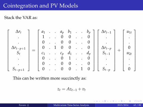
Cointegration and PV Models
Stack the VAR as:
266666666664
∆rt..
∆rt�p+1St..
St�p+1
377777777775=
266666666664
a1 . . ap b1 . . bp1 . . 0 0 . . 00 . . 0 0 . . 00 . 1 0 0 . . 0c1 . . cp d1 . . dp0 . . 0 1 . . 00 . . 0 0 . . 00 . . 0 0 . 1 0
377777777775
266666666664
∆rt�1..
∆rt�pSt�1
.
.St�p
377777777775+
266666666664
u1t..0
u2t..0
377777777775This can be written more succinctly as:
zt = Azt�1 + vt
Favero () Multivariate Time-Series Analysis 2013/2014 63 / 89

Cointegration and PV Models
The ET null puts a set of restrictions which can be written as :
g0zt =T�1
∑j=1
γjh0Aj0zt
where g0 and h0 are selector vectors for S and ∆r correspondingly ( i.e.row vectors with 2p elements, all of which are zero except for thep+1st element of g0 and the first element of h0 which are unity).For large T it must be the case that:
g0 = h0γA(I� γA)�1
which implies:g0(I� γA) = h0γA
and we have the following constraints on the individual coefficients ofVAR:
fci = �ai, 8ig , fd1 = �b1 + 1/γg , fdi = �bi, 8i 6= 1gFavero () Multivariate Time-Series Analysis 2013/2014 64 / 89

Cointegration and PV Models
Favero () Multivariate Time-Series Analysis 2013/2014 65 / 89

Cointegration and multivariate trend-shocksdecompositions
Having discussed the VECM representation for a vector of mnon-stationary variables admitting k cointegrating relationships, let uscompare it with the multivariate extension of the Beveridge�Nelsondecomposition. Consider the simple case of an I(1) vector yt featuringfirst-order dynamics and no deterministic component:
∆yt = αβ0yt�1 + ut, (3)
where α is the (m� k)matrix of loadings and β is the (m� k)matrix ofparameters in the cointegrating relationships. As yt is I(1), we canapply the Wold decomposition theorem to ∆yt to obtain the followingrepresentation:
∆yt = C (L)ut,
from which, by applying the algebra illustrated in our discussion ofthe univariate Beveridge�Nelson decomposition, we can derive thefollowing stochastic trends representation:
yt = C� (L)ut +C (1) zt,
where zt is a process for which ∆zt = ut.
Favero () Multivariate Time-Series Analysis 2013/2014 66 / 89

Cointegration and multivariate trend-shocksdecompositions
The existence of cointegration imposes restrictions on the C matrices.The stochastic trends must cancel out when the k stationary linearcombinations of the variables in yt are considered. In other words wemust have:
β0C (1) = 0.
By investigating further the relation between the VECM and thestochastic trend representations, we can give a more preciseparameterization of the matrix C (1).Note first that VECM is equivalent to:
yt =�Im + αβ0
�yt�1 + ut.
Pre-multiplying this system by β0 yields:
β0yt = β0�Im + αβ0
�yt�1 + β0ut
=�Ik + αβ0
�β0yt�1 + β0ut.
Solving this model recursively, we obtain the MA representation forthe k cointegrating relationships:
Favero () Multivariate Time-Series Analysis 2013/2014 67 / 89

Cointegration and multivariate trend-shocksdecompositions
β0yt =∞
∑i=0
�Ik + αβ0
�iβ0ut�i.
By substituting in the ECM we have the MA representation for ∆yt,
∆yt =∞
∑i=1
α�Ik + αβ0
�i�1β0ut�i + ut,
from which we have
C (1) = In � α�
β0α��1
β0.
Now note the beautiful relation (see Johansen 1995: 40),
In = β?�α0?β?
��1α0? + α
�β0α��1
β0,
where β?, α? are ((m� (m� k)) matrices of rank m� k such thatα0?α = 0, β0?β = 0.
Favero () Multivariate Time-Series Analysis 2013/2014 68 / 89

Cointegration and multivariate trend-shocksdecompositions
we haveC (1) = β?
�α0?β?
��1α0?,
andyt = C� (L)ut + β?
�α0?β?
��1 �α0?zt
�,
which shows that a system of m variables with k cointegratingrelationships features (m� k) linearly independent common trends(TR). The common trends are given by (α0?zt), while the coefficientson these trends are β? (α
0?β?)
�1. Note also that stochastic trendsdepend on a set of initial conditions and cumulated disturbances,
TRt = TRt�1 + C (1)ut.
Our brief discussion should have made clear that the VECM modeland the MA model are complementary. As a consequence, theidentification problem relevant for the vector of parameters in thecointegrating vectors β is also relevant for the vector of parametersdetermining the stochastic trends α?.Favero () Multivariate Time-Series Analysis 2013/2014 69 / 89

VECM and common trends representations
.The joint behaviour of stock prices and dividends under the dynamicdividend growth model is a good empirical example to illustrateVECM and common trend representations. Let decompose (log) stockmarket prices lpt in a permanent, information-related component, ldt,and a temporary cyclical noise component vt. :
lpt = ldt + vt,ldt = µd + ldt�1 + ut,
Dividends are the stochastic trend of stock market prices, which aremade of the permanent component and of a transitory component, vtand ut are the shocks to the transitory and the permanent componentof the system; naturally, they are orthogonal and normally andindependently distributed. Dividend and prices are cointegrated, infact they share the single unobservable common stochastic trend inthis system.
Favero () Multivariate Time-Series Analysis 2013/2014 70 / 89

VECM and common trends representations
.We obtain the VAR(1) representation by substituting for ldt in the firstequation from the second equation of :�
lptldt
�=
�µdµd
�+
�0 10 1
��lpt�1ldt�1
�+
�wtut
�,
wt = ut + vt,
from which we obtain the VECM representation:�∆lpt∆ldt
�=
�µdµd
�+
��1 10 0
��lpt�1ldt�1
�+
�wtut
�,
where
Π = αβ0. =��1 10 0
�=
�10
� ��1 1
�Favero () Multivariate Time-Series Analysis 2013/2014 71 / 89

VECM and common trends representations
.The common trend representation is derived by considering that, aslpt � ldt = vt, from which we can write :�
∆lpt∆ldt
�=
�µdµd
�+
�1 00 1
��wtut
�+
��1 10 0
��wt�1ut�1
�,
from which:�lptldt
�=
�µdµd
�t+C� (L)
�wtut
�+ C(1)zt,
where zt is a process for which ∆zt =
�wtut
�,and
Favero () Multivariate Time-Series Analysis 2013/2014 72 / 89

VECM and common trends representations
.
C(1) = β?�α0?β?
��1α0?,�
0 10 1
�=
�11
� ��0 1
� � 11
���1 �0 1
�.
Since in this application (α0?β?)�1 = 1, dividends and prices have a
single common stochastic trend. Such trend can be represented as
α0?
0BB@
µyµy
!t+
0BB@t
∑i=1
wt
t∑
i=1ut
1CCA1CCA ,
and only shocks to the permanent component of prices enter the trend.
Favero () Multivariate Time-Series Analysis 2013/2014 73 / 89

Clicker
Insert Clicker 7 here
Favero () Multivariate Time-Series Analysis 2013/2014 74 / 89
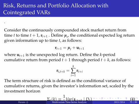
Risk, Returns and Portfolio Allocation withCointegrated VARs
.
Consider the continuously compounded stock market return fromtime t to time t+ 1, rt+1 . Define µt, the conditional expected log returngiven information up to time t, as follows:
rt+1 = µt + ut+1
where ut+1 is the unexpected log return. Define the k-periodcumulative return from period t+ 1 through period t+ k, as follows:
rt,t+k =k
∑i=1
rt+i
The term structure of risk is defined as the conditional variance ofcumulative returns, given the investor’s information set, scaled by theinvestment horizon
Σr(k) �1k
Var(rt,t+k j Dt) (4)
where Dt � σfzk : k � tg consists of the full histories of returns as wellas predictors that investors use in forecasting returns.
Favero () Multivariate Time-Series Analysis 2013/2014 75 / 89

Inspecting the mechanism: a bivariate case
Consider the continuously compounded stock market return fromtime t to time t+ 1, rt+1 . Define µt, the conditional expected log returngiven information up to time t, as follows:
rt+1 = µt + ut+1
where ut+1 is the unexpected log return. Define the k-periodcumulative return from period t+ 1 through period t+ k, as follows:
rt,t+k =k
∑i=1
rt+i
The term structure of risk is defined as the conditional variance ofcumulative returns, given the investor’s information set, scaled by theinvestment horizon
Σr(k) �1k
Var(rt,t+k j Dt) (5)
where Dt � σfzk : k � tg consists of the full histories of returns as wellas predictors that investors use in forecasting returns.
Favero () Multivariate Time-Series Analysis 2013/2014 76 / 89

Inspecting the mechanism: a bivariate case
We illustrate the econometrics of the term structure of stock marketrisk by considering a simple bi-variate first-order VAR forcontinuously compounded total stock market returns, rs
t , and the logdividend price,dpt:
(zt � Ez) = Φ1 (zt�1 � Ez) + νt
νt � N (0, Σν)
where
zt =
�rs
tdpt
�, Ez =
�Ers
Ed�p
�Φ1 =
�0 ϕ1,20 ϕ2,2
��
v1,tv2,t
�s
��00
�,
σ21 σ12
σ12 σ22
�Favero () Multivariate Time-Series Analysis 2013/2014 77 / 89

Inspecting the mechanism: a bivariate case
Given the VAR representation and the assumption of constant Σν
Vart [(zt+1 + ...+ zt+k) j Dt] = Σν + (I+Φ1)Σν(I+Φ1)0 +
(I+Φ1 +Φ21)Σν(I+Φ1 +Φ2
1)0 + ...
+(I+Φ1 + ...+Φk�11 )Σν(I+Φ1 + ...+Φk�1
1 )0
from which we can derive:
Σr(k) =1k
k�1
∑i=0
DiΣD0i
Di = I+Φ1Ξi�1 i > 0Ξi = Ξi�1 +Φi
1 i > 0D0 � I, Ξ0 � I
Favero () Multivariate Time-Series Analysis 2013/2014 78 / 89

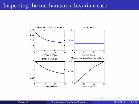
Inspecting the mechanism: a bivariate case
in our simple bivariate example, the term structure of stock marketrisk takes the form
σ2r (k) = σ2
1 + 2ϕ1,2σ1,2ψ1(k) + ϕ21,2σ2
2,2ψ2(k)
where
ψ1(k) =1k
k�2
∑l=0
l
∑i=0
ϕi2,2 k > 1
ψ2(k) =1k
k�2
∑l=0
l
∑i=0
ϕi2,2
!2
k > 1
ψ1(1) = ψ2(1) = 0
The total stock market risk can be decomposed in three components:i.i.d uncertainty, σ2
1 , mean reversion, 2ϕ1,2σ1,2ψ1(k), and uncertaintyabout future predictors, ϕ2
1,2σ22,2ψ2(k).
Favero () Multivariate Time-Series Analysis 2013/2014 79 / 89

Inspecting the mechanism: a bivariate case
Table 1: A simple bivariate VAR (1910-2008)�rs
t+1 � Ers�= ϕ12
�dpt � Edp
�+ υ1t+1�
dpt+1 � Edp�= ϕ22
�dpt � Edp
�+ ν2t+1
ϕ12(t�stat)
ϕ22(t�stat)
χ22
ϕ11=0,ϕ21=0σ1 σ2
σ12σ11σ22
adjR2rs
t+1adjR2
dpt+1
0.073 0.893 3.128 0.196 0.208 -0.844 0.02 0.79(1.71) (19.70) (0.21)
Table: The table reports coefficient estimates (with t-statistics in parentheses)and the R2 statistic for each equation. We also report the standard deviationsand correlations of residuals.
Favero () Multivariate Time-Series Analysis 2013/2014 80 / 89
Inspecting the mechanism: a bivariate case
Favero () Multivariate Time-Series Analysis 2013/2014 81 / 89

Clicker
Insert Clicker 8 here
Favero () Multivariate Time-Series Analysis 2013/2014 82 / 89

A VAR with many assets and predictors
zt = Φ0 +Φ1zt�1 + νt
where
zt =
24 r0txtst
35is a m� 1 vector. with r0t being the log real return on the asset used asa benchmark to compute excess returns on all other asset classes, , xtbeing the n� 1 vector of log excess returns on all other asset classeswith respect to to the benchmark, and st is the m� n� 1� 1 vector ofreturns predictors.νt is a m� 1 vector of innovations in asset returns and returns’predictors for which standard assumptions apply, i.e.:
νt � N (0, Σν)
where Σν is the m�m variance-covariance matrix.Favero () Multivariate Time-Series Analysis 2013/2014 83 / 89

A VAR with many assets and predictors
Note that
Σν =
24 σ20 σ00x σ00s
σ0x Σxx Σ0xsσ0s Σxs Σss
35and the unconditional mean and variances-covariance matrix ofzt,assuming that the VAR is stationary and therefore that this momentsare well-defined, can be represented as follows:
µz = (Im �Φ1)�1 Φ0
vec (Σzz) = (Im2 �Φ1 Φ1)�1 vec (Σν)
Favero () Multivariate Time-Series Analysis 2013/2014 84 / 89

A VAR with many assets and predictors
The conditional mean and variance of the cumulative asset returns atdifferent horizons are instead:
Et(zt+1 + ...+ zt+K) =
k�1
∑i=0(k� i)Φi
1
!Φ0 +
k
∑j=0
Φj1
!zt
Vart(zt+1 + ...+ zt+K) = Σν + (I+Φ1)Σν(I+Φ1)0 +
(I+Φ1 +Φ21)Σν(I+Φ1 +Φ2
1)0 + ...
+(I+Φ1 + ...+ΦK�11 )Σν(I+Φ1 + ...+ΦK�1
1 )0
Favero () Multivariate Time-Series Analysis 2013/2014 85 / 89

A VAR with many assets and predictors
Once the conditional moments of excess returns are available thefollowing selector matrix extracts for each period, k-period conditionalmoments of log real returns:
Mr =
�1 01xn 01x(m�n�1)
ιnx1 Inxn 0nx(m�n�1)
�which implies
1k
"Et
�rk
0,t+1
�Et�rk
t+1
� #=
1k
MrEt(zt+1 + ...+ zt+K)
1k
"Vart
�rk
0,t+1
�Vart
�rk
t+1
� #=
1k
MrVart(zt+1 + ...+ zt+K)M0r
Therefore after the estimation for the VAR it is possible to deriveunconditional and conditional moments for returns and excess returnsat all different investment horizons.These moments deliver the dynamics of returns and the risk ofdifferent assets across investment horizons. This information formsthe input for portfolio allocation.
Favero () Multivariate Time-Series Analysis 2013/2014 86 / 89

Mean-Variance Analysis
The starting point of mean-variance analysis is an expression for thelog-returns on the portfolio. The return on the portfolio can beapproximated as follows:
rp,t+1 = r0,t+1 + α0txt +12
α0t
�σ2
x � Σxxαt
�xt = (rt+1 � r0,t+1ι)
Σxx = Vart (rt+1 � r0,t+1ι)
σ2x = diag (Σxx)
given this definition different problems can be addressed:
Favero () Multivariate Time-Series Analysis 2013/2014 87 / 89

Mean-Variance Analysis
Campbell-Viceira(2004) show that the optimal weights ωT,t for thetangency portfolio take the following expression:
ωT,t = λf Σ�1xx
�Et (rt+1 � r0,t+1ι) +
12
σ2x
�λf =
1�Et (rt+1 � r0,t+1ι) + 1
2 σ2x�0 �
Σ�1xx�0
ι
Consider a k-period horizon we have instead:
ωT,t (k) = λf Σ�1xx (k)
�Et
�r(k)t+1 � r(k)0,t+1kι
�+
12
σ2x (k)
�λf =
1hEt
�r(k)t+1 � r(k)0,t+1kι
�+ 1
2 σ2x (k)
i0 �Σ�1
xx (k)�0
ι
Favero () Multivariate Time-Series Analysis 2013/2014 88 / 89

Mean-Variance Analysis
The typical empirical evidence produced by VAR models is thefollowing term structure of risk:
0 5 10 15 20 25 30 35 402
4
6
8
10
12
14
16
Horizon
Perc
enta
ge S
tdv
CampbellViceira model. Percentage Standard deviations
TbillsStocksBonds
Favero () Multivariate Time-Series Analysis 2013/2014 89 / 89