Multivariate Count Time Series Modelling

Konstantinos Fokianos1

1Department of Mathematics & Statistics, University of CyprusEmail: 1fokianos@ucy.ac.cy

September 21, 2021

Abstract

We review autoregressive models for the analysis of multivariate count time series. In doing

so, we discuss the choice of a suitable distribution for a vectors of count random variables.

This review focus on three main approaches taken for multivariate count time series analysis:

(a) integer autoregressive processes, (b) parameter-driven models and (c) observation-driven

models. The aim of this work is to highlight some recent methodological developments and

propose some potentially useful research topics.

Keywords: auto-correlation, covariates, copula, estimation, multivariate count distribution, prediction

1

arX

iv:2

103.

0802

8v2

[st

at.M

E]

19

Sep

2021

1 Introduction

This work reviews three main approaches that have been put forward for analysis and inference of

multivariate count time series. By now there is an extensive literature for modeling univariate count

time series, see the recent volume by Davis et al. (2016) and the review article by Davis et al. (2021),

for example. Theoretical and methodological development for multivariate count time series is still

on-going research area; see Paul et al. (2008) for a medical application, Pedeli and Karlis (2013b)

for a financial study and more recently Ravishanker et al. (2015), for a marketing application, and

Livsey et al. (2018) for an environmental study. The interested reader is referred to the review

paper by Karlis (2016), for additional literature. The aim of this work is to highlight some recent

methodological developments and propose some potentially useful research topics.

Following conventional theory, the standard venue for developing multivariate count time series

models requires specification of a joint conditional distribution. Then, likelihood inference, for a

given autoregressive model, provides estimation, testing and all type of standard output. How-

ever, choosing a joint count distribution is a challenging problem. There are numerous proposals

available in the literature generalizing univariate Poisson probability mass function (p.m.f); some

of these are reviewed in Sec. 2. The main obstacle is that the p.m.f of a multivariate ”Poisson”

discrete random vector is often of complicated functional form and therefore maximum likelihood

inference is theoretically and numerically burdensome. The choice of joint distribution for mod-

eling multivariate count data is an interesting research topic and some comments will be made

throughout this work.

The first modeling approach is based on the theory of integer autoregressive (INAR) models

and was initiated by Franke and Rao (1995) and Latour (1997). It was applied more recently by

Pedeli and Karlis (2013a,b), Scotto et al. (2014) and Darolles et al. (2019). INAR models fall

within the class of observation-driven models but because they are defined by means of thinning

operator, (see Def. 3.1 and 3.2), they deserve special attention. Estimation for INAR models is

based on least squares methodology and/or likelihood based methods. But, even for univariate

INAR models, likelihood theory is quite cumbersome, especially when dealing with higher order

autoregressive models. This methodology is reviewed in Sec. 3.

The second model class reviewed is that of parameter driven models whose dynamics–according

to the broad categorization introduced by Cox (1981)– are driven by an unobserved process. Such

models are also called state space models and have found numerous applications; see Zeger (1988),

Harvey and Fernandes (1989), Fahrmeir and Tutz (2001), West and Harrison (1997), Durbin and

2

Koopman (2000) and Fruwirth-Schnatter and Wagner (2006), among others, for contributions on

univariate time series modeling. Multivariate state space models were studied by Jørgensen et al.

(1996) and Jung et al. (2011); see also Ravishanker et al. (2014, 2015), among others, for more

recent contributions. We review these models and we illustrate that, even though their specification

is simple, they still require extensive computational efforts to be applied (using either frequentist

or Bayesian methods). Developments in this area are reviewed in Sec. 4.

Section 5 goes over observation-driven process. This is the third class of models included in this

work. Their main characteristic is that dynamics evolve according to past values of the process

plus some noise. For example, ordinary autoregressive models belong to this class. Univariate

observation–driven models for count time series have been studied by Zeger and Qaqish (1988),

Fahrmeir and Tutz (2001), Rydberg and Shephard (2000), Kedem and Fokianos (2002), Fokianos

et al. (2009), Fokianos and Tjøstheim (2011), Davis and Liu (2016), Ahmad and Franq (2016), Douc

et al. (2017), among others. There is a growing literature within the framework of multivariate

observation-driven count time series models; see Heinen and Rengifo (2007), Liu (2012), Andreassen

(2013), Ahmad (2016), Lee et al. (2018), Cui and Zhu (2018), Gourieroux and Lu (2019), Fokianos

et al. (2020), Bracher and Held (2020), Opschoor et al. (2020), Piancastelli et al. (2020), Clark

and Dixon (2021) for instance. Most of these studies are concerned with linear and/or log-linear

count time series models but other alternatives can be developed. Finally, we mention the work of

Darolles and Gourieroux (2015) who combine parameter-driven and observation-driven models to

predict the number of hedge fund defaults as a function of hedge fund past defaults.

From a personal perspective, I think that this research area is still underdeveloped and there is

ample space for exciting new developments. Some more recent works include that of Veraart (2019),

who studies continuous-time models for multivariate count time series whose marginal distribution

is infinitely divisible. This construction allows for separate modeling of serial correlation and the

cross-sectional dependence. Additional work by Hall et al. (2019) considers high-dimensional count

time series and studies the issues of inference for autoregressive parameters and the corresponding

network structure by developing a sparsity-regularized maximum likelihood estimator. Finally,

works by Zhang and Wu (2017) and Dahlhaus (1997) are potentially applicable to develop models

for high-dimensional and non-stationary data. It is envisaged that this review will motivate further

research on modeling and inference for multivariate count time series. For instance, simple questions

like prediction, diagnostics, testing or development of other more suitable models with/without

covariates will require further studies and theoretical developments. The list of references is by

no means complete but further information is given by the therein and interested readers should

3

consult them for further details.

2 A Review of Multivariate Count Distributions

We outline some parametric multivariate count distributions for independent data that have been

found useful for regression analysis. Simple properties of those models are discussed and their

connection to time series data is illustrated in Sec. 5. The goal is to show that some basic

multivariate distributions are directly applicable for fitting regression models and develop inference.

There are several alternative venues, for instance we can rely on copulas and mixture models; see

Johnson et al. (1997, Ch. 37), Joe (1997, Sec 7.2) for numerous multivariate count distributions

and Cameron and Trivedi (2013, Ch.8) for an in-depth review of multivariate count regression

models. As a general remark, joint p.m.f. of a discrete random vector often has complex functional

form which is far from being useful to develop likelihood based inference. Further recent work and

good summaries of up-to date parametric models can be found in Zhang et al. (2017), Inouye et al.

(2017), Koochemeshkian et al. (2020), among others.

A multinomial distribution, is traditionally employed for analysis of multivariate count data

by employing a multinomial logistic regression models. The multinomial distribution and the

case of Dirichlet-multinomial distribution are not included in this work (see Zhang et al. (2017)

for more). Those distributions are defined by a conditioning argument which might not extend

to time series context. It is an elementary exercise to show that if Yi is independent Poisson

distributed with mean λi for i = 1, 2, . . . , d, then the conditional distribution of (Y1, . . . Yd) given∑i Yi = y. is multinomial with parameters y. and λi/

∑j λj , for i = 1, 2, . . . , d. So, the multinomial

distribution applies to multivariate count modeling but subject to the restriction that it is supported

on {y = (y1, . . . yd)T :∑i yi = y.}. This support constraint should be considered cautiously in the

context of dependent data. Additionally, this approach provides a conditional likelihood function

for estimating regression parameters. The full likelihood function requires knowledge of the p.m.f.

of∑i Yi. Similar remark holds for Dirichlet-multinomial regression.

In what follows, we denote by Y = (Y1, . . . , Yd)T a d-dimensional vector of counts whose com-

ponents are not necessarily independent.

2.1 Multivariate Poisson Distributions

This class of distributions (Kocherlakota and Kocherlakota (1992) and Johnson et al. (1997)),

generalizes the univariate Poisson models. Put Yi = Wi+W , i = 1, 2, . . . , d where Wi ∼ Poisson(λi)

4

and W ∼ Poisson(λ0) and all W ’s are independent. Then, the joint p.m.f of Y is given

P[Y = y] = exp(−

d∑i=0

λi)( d∏

i=1

λyii

yi!

)mini yi∑k=0

( d∏i=1

(yik

))k!(

λ0∏di=1 λi

)k. (1)

The marginals, Yi, are Poisson with mean λi+λ0, for i = 1, 2, . . . , d and it holds that Cov(Yi, Yj) =

λ0 which is always positive. In addition, the parameter λ0 determines all possible pairwise corre-

lations so the resulting model is of limited use. These facts and the complicated form of (1) make

this model suitable for relatively low dimensional analysis where the marginals Yi are positively

correlated. An E-M type algorithm has been proposed by Karlis (2003) for inference but this

approach is still hard to implement when the dimension d is large. Given a vector of regressors,

say X, an appropriate regression model λi as a function of X (in terms of linear of log-linear link

function) and λ0 is taken as constant . Then using (1) likelihood inference is straightforward, at

least for low dimensions, for more see Cameron and Trivedi (2013, Ch. 8.4.1).

2.2 Mixed Poisson Models

Mixed models provide a general class of multivariate count distributions, see Marshall and Olkin

(1988). Assume that Y1, . . . , Yd are conditionally independent and Poisson distributed with E[Yi] =

λi, for i = 1, . . . , d, given λ1, . . . , λd. Suppose that the vector λ = (λ1, . . . , λd)T is distributed

according to some distribution G(λ). The mixed Poisson distribution is defined as

P[Y = y] =∫

(R+)d

[ n∏i=1

exp(−λi)λyii

yi!]dG(λ). (2)

Several choices for the mixing distribution G(·) exist. But it is always true (provided that appro-

priate moments exist) that

E[Y ] = E[λ], Var[Y ] = diag(E(λ)) + Var[λ] = diag(E(Y )) + Var[λ], (3)

because of the first equality and diag(x) denotes a diagonal matrix whose elements are given by a

vector x. A trivial example of (2) is given when G(.) is the Dirac distribution placing its mass at λ.

Then, Y is just a vector which consists of independent Poisson random variables. Finite mixtures

of multivariate Poisson distributions, with application to clustering, have been discussed by Karlis

and Meligkotsidou (2007). Another interesting case is when λ follows the d-dimensional log-normal

distribution with parameters µ = (µ1, . . . , µd)T and Σ = (σij)i,j=1,...,d. Though no closed formula

5

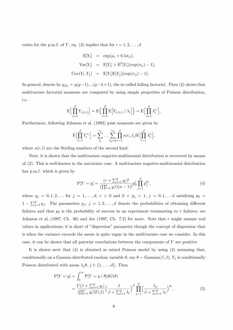
exists for the p.m.f. of Y , eq. (3) implies that for i = 1, 2, . . . , d

E[Yi] = exp(µi + 0.5σii),

Var[Yi] = E[Yi] + E2[Yi](exp(σii)− 1

),

Cov(Yi, Yj) = E[Yi]E[Yj ](exp(σij)− 1

).

In general, denote by y(k) = y(y−1)....(y−k+1), the so called falling factorial. Then (2) shows that

multivariate factorial moments are computed by using simple properties of Poisson distribution,

i.e.

E[ d∏i=1

Yi,(ri)]

= E{ d∏i=1

E[Yi,(ri) | λi

]}= E

[ d∏i=1

λrii

],

Furthermore, following Johnson et al. (1992) joint moments are given by

E[ d∏i=1

Y rii

]=

r1∑l1

. . .rd∑ld=0

d∏i=1

s(ri, li)E[ d∏i=1

λlii

],

where s(r, l) are the Stirling numbers of the second kind.

Next, it is shown that the multivariate negative-multinomial distribution is recovered by means

of (2). This is well-known in the univariate case. A multivariate negative-multinomial distribution

has p.m.f. which is given by

P[Y = y] = (r +∑di=1 yi)!

(∏di=1 yi!)(n− 1)!

pr0

d∏j=1

pyj

j , (4)

where yj = 0, 1, 2, . . . for j = 1, . . . , d, r > 0 and 0 < pj < 1, j = 0, 1, . . . d satisfying p0 =

1 −∑dj=1 pj . The parameters pj , j = 1, 2, . . . , d denote the probabilities of obtaining different

failures and thus p0 is the probability of success in an experiment terminating to r failures; see

Johnson et al. (1997, Ch. 36) and Joe (1997, Ch. 7.2) for more. Note that r might assume real

values in applications; it is short of ”dispersion” parameter though the concept of dispersion–that

is when the variance exceeds the mean–is quite vague in the multivariate case we consider. In this

case, it can be shown that all pairwise correlations between the components of Y are positive.

It is shown next that (4) is obtained as mixed Poisson model by using (2) assuming that,

conditionally on a Gamma distributed random variable θ, say θ ∼ Gamma(β, β), Yj is conditionally

Poisson distributed with mean λjθ, j ∈ {1, . . . , d}. Then

P[Y = y] =∫ ∞

0P[Y = y | θ]dG(θ)

= Γ(β +∑di=1 yi)

(∏di=1 yi!)Γ(β)

( β

β +∑di=1 λi

)β d∏j=1

( λj

β +∑di=1 λi

)yj

, (5)

6

where Γ(·) denotes the Gamma function. Obviously (4) holds. Clearly, this model implies that

the random variable θ accommodates common unobserved heterogeneity; see Munkin and Trivedi

(1999) for simulated maximum likelihood estimation for this particular class.

Recall (4). Then, given a covariate vector X, a multinomial logistic regression model (see

Agresti (2002)) is employed to link X with the probabilities pj , j = 1, 2, . . . , (d+ 1)). Furthermore,

the model can be extended to include a log-linear model for r (which can be positive real in general,

see the previous case)–for more details see Zhang et al. (2017).

2.3 Copula approaches

Copula-based construction of multivariate count distributions is an active topic of research; see

Nikoloulopoulos (2013a) and Inouye et al. (2017) for nice surveys. Copulas are useful because of

Sklar’s theorem (Sklar (1959)) which shows that marginal distributions are combined to give a

joint distribution when applying a copula, i.e. a d-dimensional distribution function all of whose

marginals are standard uniforms; the book by Nelsen (1999) gives a thorough introduction to

copulas.

Even though copulas provide an appealing methodology for constructing joint distribution func-

tions they pose challenging issues when used for discrete data analysis. First, the presence of ties in

count data (several zeroes, for example) makes them non-identifiable–Genest and Neslehova (2007),

in particular pp. 507-508–illustrate the lack of identifiability. An additional issue is that of the

likelihood function’s computationally difficulty for estimating unknown parameters. For a discrete

random vector, whose cumulative distribution function (c.d.f) is F , its p.m.f. involves 2d finite

differences of F , i.e.

P[Y = y] =∑l1=0,1

. . .∑ld=0,1

(−1)l1+...+ld P[Y1 ≤ y1 − l1, · · · , Yd ≤ yd − ld].

Computational methods using Bayesian data augmentation have been developed by Smith and

Khaled (2012), among others; the survey of Smith (2013) provides references on Bayesian method-

ology for discrete data copula modeling.

In the rest of this section I describe a different approach for employing copulas to model multi-

variate count data. The methodology is based on the work by Fokianos et al. (2020) who advanced

a particular data generating process for multivariate count time series analysis; this topic is dis-

cussed in Sec. 5. Initially, the idea is illustrated for the case of i.i.d random vectors. The intent is

to introduce a data generating process which keeps all marginal distributions of the vector Y to be

Poisson distributed and, at the same time, it allows for arbitrary dependence among them. This is

7

accomplished by appealing to elementary properties of Poisson process. An explicit account of this

construction is given by the following algorithm–recall that Yi, i = 1, 2, . . . , d is the i’th-component

of the count vector Y whose mean is λi.

1. Let U l = (U1,l, . . . , Ud,l) for l = 1, 2, . . . ,K, be a sample from a d-dimensional copula

C(u1, . . . , ud). Then Ui,l, l = 1, 2, . . . ,K follow marginally the uniform distribution on (0, 1),

for i = 1, 2, . . . , d.

2. Consider the transformation Xi,l = −logUi,l/λi, i = 1, 2, . . . , d. Then, the marginal distribu-

tion of Xi,l, l = 1, 2, . . . ,K is exponential with parameter λi, i = 1, 2, . . . , d.

3. If Xi,1 > 1 set Yi = 0, otherwise Yi = max{K :

∑Kl=1Xi,l ≤ 1

}, i = 1, 2, . . . , d. Then

Y = (Y1, . . . , Yd)T is marginally realization of a Poisson process with parameter λ.

4. Repeat steps 1-3 n times to generate a sample Y j , j = 1, 2, . . . , n.

The algorithm generates i.i.d. random vectors whose dependence among their components is

introduced by a copula structure on the waiting times of the Poisson process. In other words, the

copula is imposed on the uniform random variables generating the exponential waiting times. The

end result gives a sample of multivariate discrete random variables with Poisson marginals. The

methodology can be extended to other discrete marginal distributions provided that they can be

generated by continuous inter arrival times. For instance, suppose that Yi is marginally mixed

Poisson with mean θλi where θ satisfies E[θ] = 1. Many families of count distributions, including

the negative binomial, can be generated by this construction; see Sec. 2.2. Then steps 1-4 of the

above algorithm are still useful for generating multivariate random vectors whose marginals are not

necessarily Poisson. Indeed, generating at the first step an additional random variable θ, define

again at step 2 the waiting times by Xi,l = −logUi,l/θλi, i = 1, 2, . . . , d. Then, the distribution

of Xi is mixed exponential and therefore steps 3-4 deliver a realization of a count vector whose

marginal distribution is mixed Poisson.

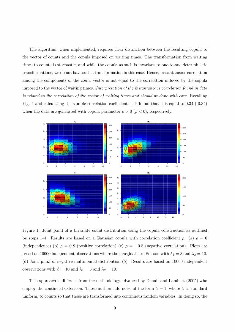
The joint p.m.f. of Y , based on the above construction, is shown in Fig. 1. Plots (a), (b) and

(c) show the case of independence, positive and negative correlation, respectively, when using a

Gaussian copula. The algorithm delivers desired marginals and, in addition, shows that all type of

different correlations can be achieved. Fig. 1(d) shows that joint p.m.f. of a negative multinomial

vector, see (5) with the same λ parameters values used for the previous algorithm and β = 10. The

positive correlation between the vector components is obvious.

8

The algorithm, when implemented, requires clear distinction between the resulting copula to

the vector of counts and the copula imposed on waiting times. The transformation from waiting

times to counts is stochastic, and while the copula as such is invariant to one-to-one deterministic

transformations, we do not have such a transformation in this case. Hence, instantaneous correlation

among the components of the count vector is not equal to the correlation induced by the copula

imposed to the vector of waiting times. Interpretation of the instantaneous correlation found in data

is related to the correlation of the vector of waiting times and should be done with care. Recalling

Fig. 1 and calculating the sample correlation coefficient, it is found that it is equal to 0.34 (-0.34)

when the data are generated with copula parameter ρ > 0 (ρ < 0), respectively.

0 2 4 6 8 10 12

05

1015

2025

(a)

x

y

0

50

100

150

200

250

300

0 2 4 6 8 10 12

510

1520

(b)

x

y

0

50

100

150

200

250

300

0 2 4 6 8 10

05

1015

20

(c)

y

0

50

100

150

200

250

300

0 2 4 6 8 10 12 14

05

1015

2025

3035

(d)

y

0

50

100

150

200

Figure 1: Joint p.m.f of a bivariate count distribution using the copula construction as outlined

by steps 1–4. Results are based on a Gaussian copula with correlation coefficient ρ. (a) ρ = 0

(independence) (b) ρ = 0.8 (positive correlation) (c) ρ = −0.8 (negative correlation). Plots are

based on 10000 independent observations where the marginals are Poisson with λ1 = 3 and λ2 = 10.

(d) Joint p.m.f of negative multinomial distribution (5). Results are based on 10000 independent

observations with β = 10 and λ1 = 3 and λ2 = 10.

This approach is different from the methodology advanced by Denuit and Lambert (2005) who

employ the continued extension. Those authors add noise of the form U − 1, where U is standard

uniform, to counts so that those are transformed into continuous random variables. In doing so, the

9

copula identifiability problem of is bypassed. An analogous approach, based on the distributional

transform which adds a random jump to the c.d.f. of the discrete variable, has been studied by

Ruschendorf (2013). An interesting decomposition of the joint p.m.f. of a discrete random vector

has been discussed by Panagiotelis et al. (2012) using the idea of pair-copula construction (Czado

(2010)) by utilizing the concept D-vine copulas (Bedford and Cooke (2001, 2002)).

Further work on copulas, in the context of generalized linear models, is given by Song (2000)

and Song et al. (2009). The latter reference employs Gaussian copulas, for multivariate regression

analysis of continuous, discrete, and mixed correlated outcomes under the generalized linear models

(GLM) framework (Nelder and Wedderburn (1972) and McCullagh and Nelder (1989)). More

recently, Yang et al. (2020) consider discrete regression models and copula estimation arguing that

inclusion of continuous covariates implies consistent estimation of the unknown copula. In addition,

Jia et al. (2021) employ a latent Gaussian process and a distributional transformation to construct

stationary univariate count time series models with flexible correlation features such that their

marginal distribution can be prespecified.

2.4 Additional models

There are additional approaches for defining a multivariate count distribution; Joe (1997, Ch.9)

and Inouye et al. (2017) review construction of multidimensional Poisson p.m.f by appealing to

full conditional distributions and Markov random fields; see Besag (1974) for the so called auto-

Poisson model. Additional models include the Sarmanov and bivariate Hurdle distributions among

others; see Cameron and Trivedi (2013, Ch. 8). These models are mentioned for completeness of

presentation but their properties have not been fully explored in the literature, to the best of my

knowledge.

3 Integer AR models

Integer Autoregressive (INAR) models deserve special consideration due to the thinning operation.

The calculus of thinning operators provides useful insight into the probabilistic properties of those

processes by employing the simple device of summing up a random number of integer-valued random

variables (see Steutel and van Harn (1979)). The case that has attracted more attention is when

the summands consist of an independent and identically distributed (iid) sequence of Bernoulli

random variables.

10

3.1 The thinning operator

Define the generalized Steutel and van Harn operator (see Latour (1997, Def. 1.1)) as follows:

Definition 3.1 Suppose that X is a non–negative integer random variable. The generalized thin-

ning operator, denoted by ◦, is defined as

α ◦X =

∑Xk=1 Ik, X > 0;

0, X = 0.

where {Ik, k ∈ N} is a sequence of iid integer random variables–independent of X–with mean α and

variance β.

The sequence {Ik, k ∈ N} is called counting series. If {Ik} is an iid sequence of Bernoulli random

variables, then α ◦X counts the number of successes in a random number of Bernoulli trials where

the probability of success α remains constant throughout the experiment so that given X, α◦X is a

binomial random variable with parameters X and α. In this case, we call the thinning operator as

binomial thinning operator. General thinning operators are discussed by Davis et al. (2021, Sec.2)

and Joe (2016), among others.

Numerous properties can be proved for the thinning operator, for instance it can be shown that

E [α ◦X | X] = αX, E [α ◦X] = αE [X], Var [α ◦X | X] = βX and Var [α ◦X] = α2Var [X] +

βE [X], provided that appropriate moments of X exist.

Definition 3.1 can be extended to a non-negative integer d-dimensional random vectors. For

i, j = 1, 2, . . . , d, define {Iij;k, k ∈ N} an array of counting series such that E[Iij ] = αij and Var[Iij ] =

βij . Let A = (αij), B = (βij) be the corresponding d × d matrices. Then, Definition 3.1 can be

extended as follows:

Definition 3.2 Suppose that X = (X1, X2, . . . , Xd)T is d-dimensional integer-valued random vec-

tor with all components being non-negative and denote by A◦ = (αij◦) a d× d matrix of thinning

operators whose each element is given by Def. 3.1 with corresponding array of counting series

{Iij;k, k ∈ N}. Then the multivariate thinning operator is defined as

A ◦X =

∑dj=1 α1j ◦Xj

...∑dj=1 αdj ◦Xj

.

Similar to the univariate case, it can be shown that E[A ◦ X] = AE[X] and Var[A ◦ X] =

diag(BE[X]) +ACov[X]AT .

11

3.2 The multivariate INAR model

The multivariate thinning operator serves as basic tool to develop multidimensional integer AR

models (abbreviated by MINAR) of order p. A d-dimensional time series {Yt, t ∈ Z} is called

multivariate INAR(p) process if it satisfies

Yt =∑pi=1Ai ◦ Yt−i + εt, (6)

where {εt, t ∈ Z} is a sequence of iid integer-valued random vectors with mean E[εt] = µε and

Var[εt] = Σε which is independent of all thinning operators Ai, i = 1, 2, . . . , p and Ap 6= 0. Denote by

Id the d-dimensional identity matrix. Provided that the roots of polynomial det(Id−A1z−· · ·Apzp)

are all located outside the unit circle, then Latour (1997, Prop. 3.1) shows that there exists an

almost surely unique integer-valued strictly stationary process that satisfies (6) and such that εt is

independent of Ys, s < t. For the case of d = 1, this condition is equivalent to 0 <∑pi=1Ai < 1,

see Du and Li (1991). The univariate INAR(p) processes have been introduced by Al-Osh and

Alzaid (1987), Alzaid and Al-Osh (1990). In the same vein, multivariate INAR moving average

(MINARMA) models can be defined but they will not be discussed any further.

We assume the stability condition for MINAR(p) processes holds true. Recall (6) and consider

the special case of p = 1. By taking expectations in both sides of (6), E[Yt] = (Id − A1)−1µε.

Multiplying both sides of (6) by Yt+h and taking expectations, it follows that Cov(Yt, Yt+h) =

Ah1Var(Yt), where Var(Yt) = A1Var(Yt)AT1 + diag(BE[Yt]) + Σε for h = 0,±1,±2 · · · . As a final

remark, Latour (1997, Prop. 4.1) shows that a MINAR(p), which satisfies the stability condition

discussed earlier, has identical second order properties with an ordinary vector AR(p) (VAR) model

(see Tsay (2014)). Consider again the case p = 1 for (6). Then {Yt} is represented by a VAR(1)

process of the form

Yt = ω +A1Yt−1 + ζt (7)

where {ζt} is a white noise process with covariance matrix Σζ = diag(BE[Yt]) + Σε and ω = E[Yt].

This fact has important consequences on estimation. For instance least squares estimators (LSE)

directly applies to this class of models but subject to restriction that all unknown coefficients are

positive.

3.3 Estimation

Besides LSE, likelihood estimation has been also developed for estimating the unknown parameters

of the model (6). Both methods are discussed next by assuming that Y1, . . . , Yn is a sample from

12

a MINAR(1) model–this is done mostly for convenience.

LSE are computed and studied by using (7). Let

Y︸︷︷︸(n−1)×d

= X?︸︷︷︸(n−1)×(d+1)

β︸︷︷︸(d+1)×d

+ Z︸︷︷︸(n−1)×d

where the i’th row of Y , X? and Z is given by Y Ti+1, (1, Y T

i ) and ζTi , i = 1, 2, . . . , (n−1), respectively.

The regression matrix parameter is denoted by β, i.e. β = (ω,A1)T . Then the LSE of β is denoted

by β and is equal to

β =(X?TX?

)−1X?TY =

( n∑t=2

1 Y Tt

Yt YtYTt

)−1( n∑t=2

Y Tt

Yt−1YTt

). (8)

Based on this define the residual matrix Z = Y −X?β to obtain an estimator of Σζ by

Σζ = 1n− d− 2 ZZ

T ,

where the numerator n−d−2 = (n−1)− (d+ 1) is equal to the effective degrees of freedom minus

the number of parameters estimated for each component series. More precisely, it can be shown

that E[β] = β and E[Σζ ] = Σζ . Moreover, as n→∞, and assuming suitable regularity conditions

are fulfilled

√n vec

(β − β

) D=⇒ N(0,Σζ ⊗H−1),

where vec(.) denotes the vec operator, ⊗ is the Kronecker product and the (d+ 1)× (d+ 1) matrix

H is the limit (in probability) of X?TX?/n. A rigorous statement is developed along the lines

of Latour (1997) and Lutkepohl (2005, Lemma 3.1). This result holds when the true parameters

belong to the interior of parameter space employing unconstrained optimization. The asymptotic

distribution of LSE, under the constraint that all elements of the matrix A1 are positive, is an open

problem.

Besides LSE, conditional likelihood estimation is developed (recall again (6) with p = 1) by

maximizing the likelihood function

L(β) =n∏t=1

Pβ[Yt = yt | Yt−1 = yt−1],

when imposing a multivariate distribution on the error term εt. In general the conditional transition

is given by the d-dimensional convolution

Pβ[Yt = yt | Yt−1 = yt−1] =yt∑k=0

Pβ[A1 ◦ Yt−1 = yt − k]P [εt = k].

13

Both the above equation implies that the log-likelihood function is given by

l(β) ≡ logL(β) =n∑t=1

log( yt∑k=0

Pβ[A1 ◦ Yt−1 = yt − k]P [εt = k]).

This short discussion shows that the task of computing the log-likelihood function is daunting even

in the simple case p = 1. Some simplifications occur when we assume that the matrix A1 is diagonal

and by applying pairwise likelihood methodology as in Pedeli and Karlis (2013a). Such an approach

can deliver some insights for data analysis but it will be difficult to be justified for multivariate

dynamic systems. Generally, likelihood methods are not suitable for this class of models because

of their complicated structure. The problem complexity increases when both p and d grow but

sparsity ideas (see Hastie et al. (2015)) will be helpful.

3.4 Prediction

Consider again the case of model (6) for p = 1. We briefly discuss prediction for this particular

case to overcome cumbersome notation. Similar to the case of VAR(p) models, a MINAR(p) model

is written as a ”big” MINAR(1) so these results suffice to develop a general point of view.

The one-step ahead predictor of the MINAR(1) process is easily calculated by

E[Yt+1 | Yt] = E [A1 ◦ Yt + εt | Yt] = A1Yt + µε.

Therefore, by recursion

E[Yt+h | Yt] = Ah1Yt +(Id +A1 + · · ·+Ah−1

1)µε.

Define V (h) = Var[Yt+h | Yt]. Then

V (1) = Var(A1 ◦ Yt + εt | Yt

)= diag(BE[Yt]) + Σε.

The law of total variance shows that

V (h) = E[Var

(Yt+h | Yt+1

)| Yt

]+ Var

[E(Yt+h | Yt+1

)| Yt

]= E[V (h− 1)] +Ah−1

1 V (1)(Ah−11 )T

Provided that A1 is diagonal, some simplifications of the previous formulas have been proved by

Pedeli and Karlis (2013b). The complexity of prediction problem increases as both dimension and

model order increase. In addition, care should be taken when unknown parameters are replaced by

their estimators.

14

Closing this section, we mention that properties of multivariate INAR models are well un-

derstood for low-dimensional data and under tangible assumptions. It is interesting to consider

properties of the multivariate thinning operator in high-dimensions and investigate the problem of

estimation and prediction.

4 Parameter-Driven Models

A parameter driven model, according to classification introduced by Cox (1981), is a time series

driven by an unobserved process (as opposed to past process values; see Sec 5). For multivariate

count series, state-space models were studied in Jørgensen et al. (1999) and Jung et al. (2011); see

Ravishanker et al. (2014), and Ravishanker et al. (2015), among others, for more recent contribu-

tions. The approaches that have been taken for estimation are based either on likelihood or full

Bayesian methods. We review some of these works.

The model proposed by Jørgensen et al. (1999), is closely related to the theory of mixed Poisson

distributions, see Sec. 2.2. It assumes that the conditional distribution of the i’th component of the

multivariate count series at time t, Yi,t, given an unobserved univariate time-varying process 1 θt,

is Poisson distributed with mean ai,tθt such that ai,t = exp(cTt αi), where ct are k-dimensional time-

varying covariate vectors and αi are k-dimensional regression parameters, i = 1, . . . , d. Assume

that θ0 = 1 and the conditional distribution of θt given θt−1 is Gamma with mean btθt−1 and a

squared coefficient of variation of form σ2/θt−1. The parameters bt depend on the so called long–

term covariates zt through bt = exp(∆zTt β), where ∆zt = zt − zt−1 and z0 = 0, σ2 denotes a

dispersion parameter and β is regression coefficient. It can be shown that

E[θt] = b1 . . . bt

which implies that log(E[θt]) = z′tβ. In addition, for h ≥ 0,

Var(θt) = φtE[θt]σ2, Cov(θt, θt+h) = φtE[θt+h]σ2,

where φt = bt + btbt−1 + btbt−1 . . . b1. Set at = (a1,t, . . . , ad,t)T and At = Diag(a1,t, . . . , ad,t). Then

(compare with (3) when ai,t = 1 for all i and t)

E[Yt] = at E[θt], Var(Yt) = AtE[θt] + ataTt φtσ

2E[θt].

1For this part of the text, I replace the notation λt by θt because it denotes a univariate time-varying mean

process.

15

This last result shows that the variance matrix of Yt consists of two components; (a) a Poisson

variance and (b) a type of ”overdispersion” component. The authors discuss Kalman prediction

and filtering, for the log-linear model E[Yi,t] = exp(cTt αi + zTt β), relying on previous calculations.

The above model is closely related to the model of Jung et al. (2011) which in turn generalizes

that of Wedel et al. (2003) who developed a comprehensive class of factor models for multivariate

truncated count data. The former authors assume that Yi,t, conditionally on λi,t, are independent

Poisson distributed random variables with mean λi,t, i = 1, 2, . . . , d and for all t. By considering

the d-dimensional time-varying vector process λt = (λ1,t, . . . , λd,t)T , it is assumed that

log λt = ω + Γft,

where ω is d-dimensional vector of parameters, Γ is a d × s matrix of factor loadings, ft is an

s-dimensional vector of latent random factors and the log(.) function is taken componentwise.

Further, the components of ft are decomposed to similar subsets which are assumed to follow

independently Gaussian AR(1) model. Jung et al. (2011) develop estimation under Poisson and

Negative binomial distribution by employing efficient importance sampling and apply this method-

ology to numbers of trades, in 5-min intervals, for five New York Stock Exchange stocks from two

industrial sectors.

Similarly, Wang and Wang (2018) assume that E[Yi,t] = E[λi,t]εi,t, where εi,t is the i’th compo-

nent of a d-dimensional hidden process εt such that E[εi,t] = 1 (see also Zeger (1988), Davis and

Wu (2009) and Christou and Fokianos (2014)). This assumption implies that

Cov[Yi,t, Yj,u] = E[λi,t]E[λj,u]Cov[εi,t, εj,u],

for any t, u and i 6= j or t 6= u and all i, j. Effectively the autocovariance function of the hidden

process is identical to the autocovariance function of the standardized process Yi;t/E[λi,t]. Wang

and Wang (2018) assume further that E[ai,t] = exp(cTt αi) using the previous notation. To reduce

the dimensionality of hidden process εt, it is assumed to satisfy εt = Γft as in Jung et al. (2011)

but with s = dim(ft) unknown. Correlation is taken into account by this construction since the

dynamics of ft drive the time-evolution of εt. Inference proceeds in two steps: (a) pseudo-maximum-

likelihood estimation for regression coefficients and (b) identification of common factor(s) utilizing

eigenanalysis on a positive definite matrix.

In a related article, Zhang, Chen, and Li (2017) discuss a model which is based on the the

multivariate lognormal mixture Poisson distribution (see Sec. 2.2) and allows for serial correlations

by assuming that the Poisson mean vector is a latent process driven by a nonlinear autoregres-

sive model. The authors employ Monte Carlo Expectation Maximization algorithm together with

16

particle filtering and smoothing methods to develop inference. Similarly, Al-Wahsh and Hussein

(2020) motivated by an application concerning asthma related visits to emergency rooms, consider

a hidden autoregressive process which drives the dynamics of a positively correlated bivariate time

series of counts whose conditional distribution is assumed to be the multivariate Poisson distri-

bution (1). The authors use a Bayesian data cloning approach to compute maximum likelihood

estimators and their standard errors.

From a fully Bayesian point of view, Aktekin et al. (2018) (see also Gamerman et al. (2013)) as-

sume that Yi;t are independent, conditionally on univariate parameters αi and a process εt, Poisson

distributed with mean αiθt. The parameter αi are individual specific rates and εt is a common pro-

cess that drives the dynamics of the observed process and satisfies εt = (εt−1/γ)dt, where γ ∈ (0, 1)

and dt are independent Beta random variables with suitable parameters. The authors study, in

addition, a negative binomial model and they implement inference by particle learning algorithm.

Another fully Bayesian approach is that of Berry and West (2020) who introduce models, within

the framework of dynamic GLM (see West and Harrison (1997)), that allow use of time-varying

covariates for binary and Poisson conditionally distributed time series. The recent review article

by West (2020) gives further insight for Bayesian modeling of multivariate count time series. Other

works, along these lines include Serhiyenko (2015), Ravishanker et al. (2014), Ravishanker et al.

(2015). The previous articles and the recent work of Davis et al. (2021) give further references and

list other approaches.

5 Observation-Driven Models

In this section, we discuss observation-driven models, that is processes whose dynamics are driven

by past observations plus noise. A convenient model would postulate a multivariate conditional

count distribution to the observed process such that likelihood inference is feasible. But the discus-

sion in Sec. 2 illustrated the obstacles of choosing appropriate count distribution. In this section

we will be studying the GLM approach. It will be argued that this framework generalizes the tradi-

tional ARMA methodology (see Shumway and Stoffer (2011) for example) to the count time series

framework. Model fitting is based, in general, on quasi-likelihood inference; Godambe (1991) Heyde

(1997); therefore testing, diagnostics and all type of likelihood arguments are directly applicable

for this case.

17

5.1 Linear Models

To initiate the discussion, consider the standard VAR(1) model, but in the context of a multivariate

Poisson autoregression as it is discussed next. Denote by Ft the σ–field generated by all past

values of the process {Ys, s ≤ t}. Let {λt = (λi,t), i = 1, 2, . . . , d, t ∈ Z} be the corresponding

d-dimensional intensity process, vis. E[Yt | Ft−1] = λt. The univariate linear autoregressive model

discussed by Rydberg and Shephard (2000), Heinen (2003), Ferland et al. (2006) and Fokianos

et al. (2009), among others, serves as basic building block to construct a multivariate Poisson

linear VAR(1) process by defining

Yi,t | Ft−1 ∼ marginally Poisson(λi,t), λt = ω +B1Yt−1, (9)

where ω is a d-dimensional vector and B1 is a d× d unknown matrices. The elements of ω and B1

are assumed to be positive such that λi,t > 0. for all i and t. It is instructive to consider (9) in

more detail. For the simple case d = 2, it implies that

λ1t = ω1 + b111 Y1,(t−1) + b12

1 Y2,(t−1),

λ2t = ω2 + b211 Y1,(t−1) + b22

1 Y2,(t−1),

where ωi is the i’th element of ω and bij1 is the (i, j)th element of B1. Then setting b121 = 0 implies

that the past values of Y2,t do not affect the evolution of Y1,t. Similarly, b211 = 0 shows that past

values of Y1,t do not affect the evolution of Y2,t. These arguments extend naturally to the case

d > 2.

Generating data using (9) is accomplished by imposing (1), for instance; see Liu (2012) and

Pedeli and Karlis (2013b) for some examples. But the discussion in Sec. 2 shows the challenges

of fitting model (9) to data assuming a bivariate Poisson (and more generally multivariate Pois-

son) distribution. To overcome this challenge we appeal to copulas–but other suitable p.m.f are

applicable–by introducing a joint distribution constructed by utilizing the data generating process

described in Sec. 2.3 but taking into account (9). The algorithm is repeated for completeness of

presentation. Let λ0 be a starting value and assume that ω, B1 are given. Then

1. Let U l = (U1,l, . . . , Ud,l) for l = 1, 2, . . . ,K, be a sample from a d-dimensional copula

C(ud, . . . , ud). Then Ui,l, l = 1, 2, . . . ,K follow marginally the uniform distribution on (0, 1),

for i = 1, 2, . . . , d.

2. Consider the transformation Xi,l = −logUi,l/λi,0, i = 1, 2, . . . , d. Then, the marginal distri-

bution of Xi,l, l = 1, 2, . . . ,K is exponential with parameter λi,0, i = 1, 2, . . . , d.

18

3. If Xi,1 > 1, set Yi,0 = 0, otherwise Yi,0 = max{K :

∑Kl=1Xi,l ≤ 1

}, i = 1, 2, . . . , d. Then

Y0 = (Y1,0, . . . , Yd,0)T is marginally a realization of a Poisson process with parameter λ0.

4. Use (9) to obtain λ1.

5. Return back to step 1 to obtain Y1, and so on.

−1.0 −0.5 0.0 0.5 1.0

0.00

0.10

0.20

0.30

ρ

Cov

(Y1t

, Y1(

t+1)

)

−1.0 −0.5 0.0 0.5 1.0

0.25

0.30

0.35

ρ

Cov

(Y1t

, Y2(

t+1)

)

−1.0 −0.5 0.0 0.5 1.0

0.30

0.34

0.38

0.42

ρ

Cov

(Y2t

, Y1(

t+1)

)

−1.0 −0.5 0.0 0.5 1.0

0.0

0.1

0.2

0.3

ρ

Cov

(Y2t

, Y2(

t+1)

)

Figure 2: Lag 1 autocorrelation matrix of a bivariate count time series as a function of the Gaussian

copula parameter ρ. Results are based on 5000 data points.

Figure 2 shows plots of the sample autocorrelation matrix Cov(Yt, Yt+1) where Yt is a bivariate

count time series generated using the above algorithm and model (9) with a Gaussian copula having

parameter ρ. The plot reinforces the point raised in Sec. 2.3 where it is noted that interpretation

of the instantaneous correlation found in data is related to the correlation of the vector of waiting

times and should be done with care. This simple example shows that, as ρ varies between -1 and 1,

all the lag 1 correlation functions do not exceed 0.45. But the plot also shows that this approach

takes into account properly the correlation found in data because by varying the parameter ρ we

obtain different type of autocorrelation matrices.

19

It is worth pointing out that this approach is different when compared to the work of Heinen and

Rengifo (2007). These authors replace the original counts by employing the continued extension

method of Denuit and Lambert (2005), as it was discussed in Sec. 2.3. The continued extension

method of Heinen and Rengifo (2007) has been investigated in a simulation study by Nikoloulopou-

los (2013b). Other copula-based models for multivariate count distributions with serial dependence

are discussed in Joe (1997, Ch. 8).

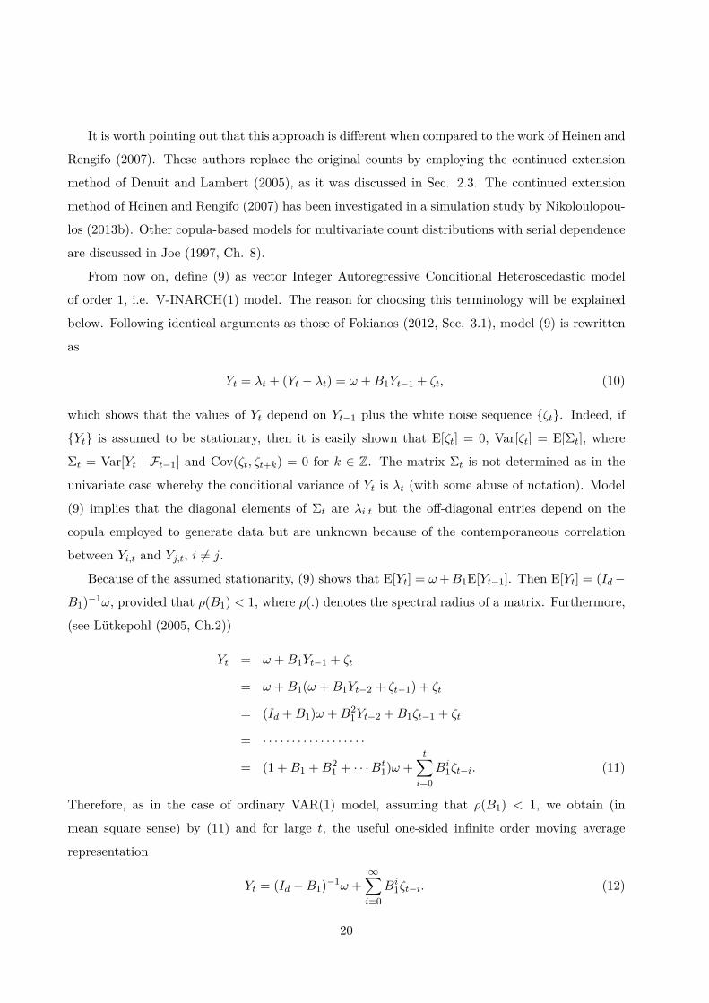
From now on, define (9) as vector Integer Autoregressive Conditional Heteroscedastic model

of order 1, i.e. V-INARCH(1) model. The reason for choosing this terminology will be explained

below. Following identical arguments as those of Fokianos (2012, Sec. 3.1), model (9) is rewritten

as

Yt = λt + (Yt − λt) = ω +B1Yt−1 + ζt, (10)

which shows that the values of Yt depend on Yt−1 plus the white noise sequence {ζt}. Indeed, if

{Yt} is assumed to be stationary, then it is easily shown that E[ζt] = 0, Var[ζt] = E[Σt], where

Σt = Var[Yt | Ft−1] and Cov(ζt, ζt+k) = 0 for k ∈ Z. The matrix Σt is not determined as in the

univariate case whereby the conditional variance of Yt is λt (with some abuse of notation). Model

(9) implies that the diagonal elements of Σt are λi,t but the off-diagonal entries depend on the

copula employed to generate data but are unknown because of the contemporaneous correlation

between Yi,t and Yj,t, i 6= j.

Because of the assumed stationarity, (9) shows that E[Yt] = ω+B1E[Yt−1]. Then E[Yt] = (Id−

B1)−1ω, provided that ρ(B1) < 1, where ρ(.) denotes the spectral radius of a matrix. Furthermore,

(see Lutkepohl (2005, Ch.2))

Yt = ω +B1Yt−1 + ζt

= ω +B1(ω +B1Yt−2 + ζt−1) + ζt

= (Id +B1)ω +B21Yt−2 +B1ζt−1 + ζt

= · · · · · · · · · · · · · · · · · ·

= (1 +B1 +B21 + · · ·Bt

1)ω +t∑i=0

Bi1ζt−i. (11)

Therefore, as in the case of ordinary VAR(1) model, assuming that ρ(B1) < 1, we obtain (in

mean square sense) by (11) and for large t, the useful one-sided infinite order moving average

representation

Yt = (Id −B1)−1ω +∞∑i=0

Bi1ζt−i. (12)

20

In addition

ΓY (h) ≡ Cov(Yt, Yt+h) =∞∑i=0

Bi+h1 E[Σt](Bi)T , h ≥ 0,

Several other results are readily available because of (10), see Lutkepohl (2005) or Tsay (2014).

Generalizations of (9), such as the V-INARCH(p) model

λt = ω +p∑i=1

BiYt−i,

or the vector V-INGARCH(p, q) (where ”G” stands for Generalized)

Yi,t | Ft−1 is marginally Poisson(λi,t), λt = ω +p∑i=1

BiYt−i +q∑j=1

Ajλt−j , (13)

where (Aj)qj=1, (Bi)pi=1 are d× d unknown matrices and all the elements of ω, (Aj)qj=1, (Bi)pi=1 are

positive such that λi,t > 0. for all i and t, are studied along the previous arguments. The abbre-

viation ”INGARCH” for model (13) just indicates its structural connection to ordinary GARCH

model, Bollerslev (1986), because each component of the vector process Yt is distributed as a Pois-

son random variable. But the mean of a Poisson random variable equals its variance; therefore

the structure of (13) bears some resemblance to that of a multivariate GARCH model, see Francq

and Zakoıan (2010). Though the term ”V-INGARCH” does not reflect accurately the true data

generating process it will be used as a generalization of the terminology introduced for univariate

models by Ferland et al. (2006).

It is proved that (13) is a VARMA(max(p, q), q) process. Recall that ζt = Yt − λt. Then

assuming first order stationarity of Yt and taking expectations on both sides of (13), we obtain

that E[Yt] = (Id −∑pi=1Ai −

∑qj=1Bj)−1ω, provided that ρ(

∑pi=1Ai +

∑qj=1Bj) < 1. Then, by

manipulating (10) but for model (13), it is easily shown that

(Yt − E[Yt]

)=

max(p,q)∑i=1

(Ai +Bi

)(Yt−i − E[Yt]

)+ ζt −

q∑j=1

Ajζt−j , (14)

where we set Ai = 0d if q < p for i = q + 1, . . . , p or Bi = 0d if q > p for i = p + 1, . . . , q. In

the case of p = q = 1 the one-sided MA(∞) is given by Yt = µ +∑∞j=0 Φjζt−j with Φ0 = Id and

Φj = (A1 +B1)j−1B1, for j ≥ 1, a fact that shows for any h > 0

ΓY (h) =∞∑j=0

(A1 +B1

)j+h−1B1E[Σt]BT

1(AT1 +BT

1)j+h−1

,

by using properties of the linear multivariate processes.

21

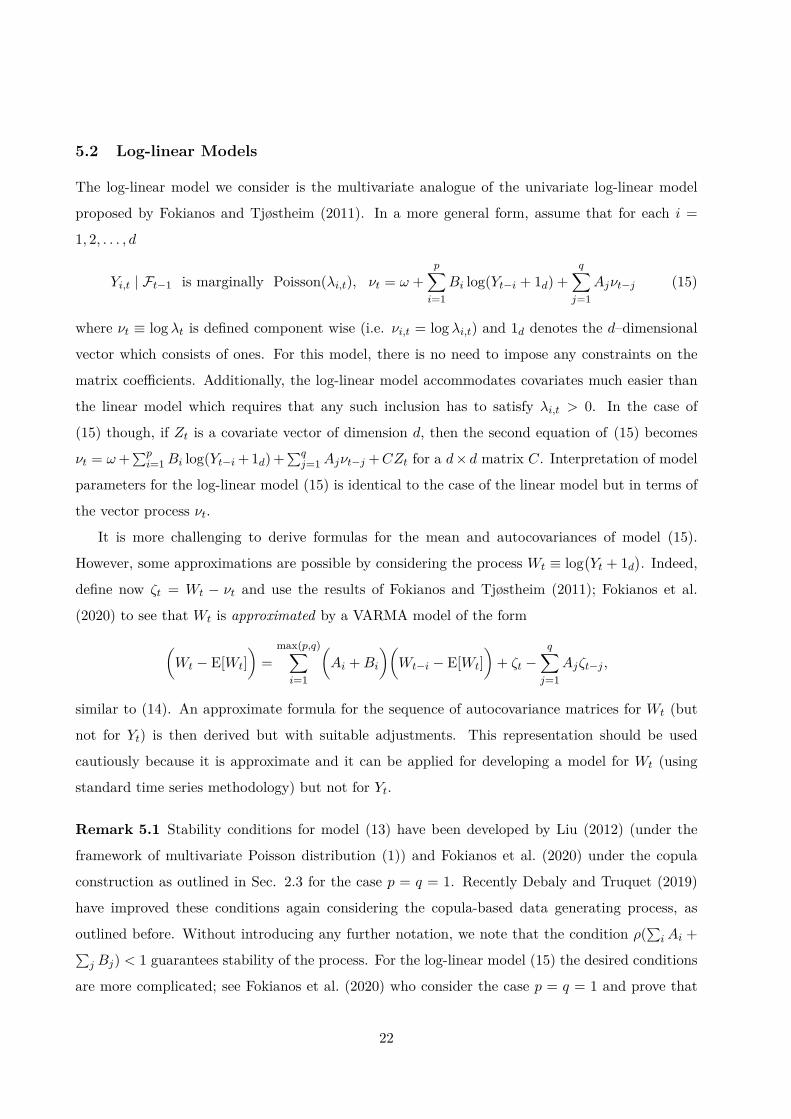
5.2 Log-linear Models

The log-linear model we consider is the multivariate analogue of the univariate log-linear model

proposed by Fokianos and Tjøstheim (2011). In a more general form, assume that for each i =

1, 2, . . . , d

Yi,t | Ft−1 is marginally Poisson(λi,t), νt = ω +p∑i=1

Bi log(Yt−i + 1d) +q∑j=1

Ajνt−j (15)

where νt ≡ log λt is defined component wise (i.e. νi,t = log λi,t) and 1d denotes the d–dimensional

vector which consists of ones. For this model, there is no need to impose any constraints on the

matrix coefficients. Additionally, the log-linear model accommodates covariates much easier than

the linear model which requires that any such inclusion has to satisfy λi,t > 0. In the case of

(15) though, if Zt is a covariate vector of dimension d, then the second equation of (15) becomes

νt = ω+∑pi=1Bi log(Yt−i + 1d) +

∑qj=1Ajνt−j +CZt for a d× d matrix C. Interpretation of model

parameters for the log-linear model (15) is identical to the case of the linear model but in terms of

the vector process νt.

It is more challenging to derive formulas for the mean and autocovariances of model (15).

However, some approximations are possible by considering the process Wt ≡ log(Yt + 1d

). Indeed,

define now ζt = Wt − νt and use the results of Fokianos and Tjøstheim (2011); Fokianos et al.

(2020) to see that Wt is approximated by a VARMA model of the form

(Wt − E[Wt]

)=

max(p,q)∑i=1

(Ai +Bi

)(Wt−i − E[Wt]

)+ ζt −

q∑j=1

Ajζt−j ,

similar to (14). An approximate formula for the sequence of autocovariance matrices for Wt (but

not for Yt) is then derived but with suitable adjustments. This representation should be used

cautiously because it is approximate and it can be applied for developing a model for Wt (using

standard time series methodology) but not for Yt.

Remark 5.1 Stability conditions for model (13) have been developed by Liu (2012) (under the

framework of multivariate Poisson distribution (1)) and Fokianos et al. (2020) under the copula

construction as outlined in Sec. 2.3 for the case p = q = 1. Recently Debaly and Truquet (2019)

have improved these conditions again considering the copula-based data generating process, as

outlined before. Without introducing any further notation, we note that the condition ρ(∑iAi +∑

j Bj) < 1 guarantees stability of the process. For the log-linear model (15) the desired conditions

are more complicated; see Fokianos et al. (2020) who consider the case p = q = 1 and prove that

22

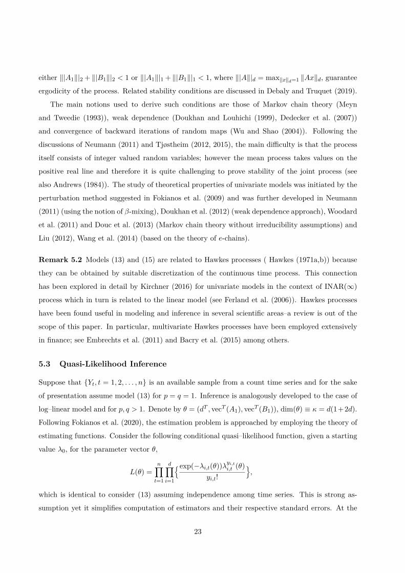
either ‖|A1‖|2 + ‖|B1‖|2 < 1 or ‖|A1‖|1 + ‖|B1‖|1 < 1, where ‖|A‖|d = max‖x‖d=1 ‖Ax‖d, guarantee

ergodicity of the process. Related stability conditions are discussed in Debaly and Truquet (2019).

The main notions used to derive such conditions are those of Markov chain theory (Meyn

and Tweedie (1993)), weak dependence (Doukhan and Louhichi (1999), Dedecker et al. (2007))

and convergence of backward iterations of random maps (Wu and Shao (2004)). Following the

discussions of Neumann (2011) and Tjøstheim (2012, 2015), the main difficulty is that the process

itself consists of integer valued random variables; however the mean process takes values on the

positive real line and therefore it is quite challenging to prove stability of the joint process (see

also Andrews (1984)). The study of theoretical properties of univariate models was initiated by the

perturbation method suggested in Fokianos et al. (2009) and was further developed in Neumann

(2011) (using the notion of β-mixing), Doukhan et al. (2012) (weak dependence approach), Woodard

et al. (2011) and Douc et al. (2013) (Markov chain theory without irreducibility assumptions) and

Liu (2012), Wang et al. (2014) (based on the theory of e-chains).

Remark 5.2 Models (13) and (15) are related to Hawkes processes ( Hawkes (1971a,b)) because

they can be obtained by suitable discretization of the continuous time process. This connection

has been explored in detail by Kirchner (2016) for univariate models in the context of INAR(∞)

process which in turn is related to the linear model (see Ferland et al. (2006)). Hawkes processes

have been found useful in modeling and inference in several scientific areas–a review is out of the

scope of this paper. In particular, multivariate Hawkes processes have been employed extensively

in finance; see Embrechts et al. (2011) and Bacry et al. (2015) among others.

5.3 Quasi-Likelihood Inference

Suppose that {Yt, t = 1, 2, . . . , n} is an available sample from a count time series and for the sake

of presentation assume model (13) for p = q = 1. Inference is analogously developed to the case of

log–linear model and for p, q > 1. Denote by θ = (dT , vecT (A1), vecT (B1)), dim(θ) ≡ κ = d(1+2d).

Following Fokianos et al. (2020), the estimation problem is approached by employing the theory of

estimating functions. Consider the following conditional quasi–likelihood function, given a starting

value λ0, for the parameter vector θ,

L(θ) =n∏t=1

d∏i=1

{exp(−λi,t(θ))λyi,t

i,t (θ)yi,t!

},

which is identical to consider (13) assuming independence among time series. This is strong as-

sumption yet it simplifies computation of estimators and their respective standard errors. At the

23

same time, it guarantees consistency and asymptotic normality of the maximizer. Furthermore, the

dependence structure in (13) and (15) is taken into account through because of the dependence of

the likelihood function on the matrices A1 and B1; see Fokianos et al. (2020) for more. The quasi

log-likelihood function is equal to

l(θ) =n∑t=1

d∑i=1

(yi,t log λi,t(θ)− λi,t(θ)

).

We denote by θ ≡ arg maxθ l(θ), the QMLE of θ. The score function is given by

Sn(θ) =n∑t=1

d∑i=1

( yi,tλi,t(θ)

− 1)∂λi,t(θ)

∂θ=

n∑t=1

∂λTt (θ)∂θ

D−1t (θ)

(Yt − λt(θ)

)(16)

where ∂λt/∂θT is a d×κ matrix and Dt is the d×d diagonal matrix with the i’th diagonal element

equal to λi,t(θ), i = 1, 2, . . . , p. Furthermore

∂λt∂dT

= Id +A1∂λt−1∂dT

,

∂λt∂ vecT (A1) = (λt−1 ⊗ Id)T +A1

∂λt−1∂ vecT (A1) ,

∂λt∂ vecT (B1) = (Yt−1 ⊗ Id)T +A1

∂λt−1∂ vecT (B1) .

The Hessian matrix is given by

Hn(θ) =n∑t=1

p∑i=1

yi;tλ2i,t(θ)

∂λi,t(θ)∂θ

∂λi,t(θ)∂θT

−n∑t=1

p∑i=1

( yi,tλi,t(θ)

− 1)∂2λi,t(θ)∂θ∂θT

. (17)

Therefore, the conditional information matrix is equal to

Gn(θ) =n∑t=1

∂λTt (θ)∂θ

D−1t (θ)Σt(θ)D−1

t (θ)∂λt(θ)∂θT

, (18)

where the matrix Σt(·) denotes the true covariance matrix of the vector Yt. In case that the process

{Yt} consists of uncorrelated components then Σt(θ) = Dt(θ). In the case that of A1 being a

diagonal matrix then θ is computed by equation by equation using existing software.

Under suitable conditions, Fokianos et al. (2020) show that

√n(θ − θ0) d−→ N(0, H−1GH−1)

where the matrices H and G are defined by the limits (in probability) of (17) and (18), respectively.

The same result is true for the log-linear model (15); details are omitted. To estimate the copula

parameter, it is desirable to compare the conditional distribution of Yt | λt to that of Y ∗t | λt, where

Y ∗t is a count time series generated by a suitable choice of a copula. There are several ways of

24

comparing such distributions and this topic is still under investigation. In Fokianos et al. (2020) an

initial approach, based on the newly developed concept of local Gaussian correlation (see Berentsen

et al. (2014)) was shown to be satisfactory. But the problem of estimating the copula parameter

remains unexplored; see Debaly and Truquet (2021) for recent progress in the framework of mixed

time series models.

Remark 5.3 Equation (16) motivates a more general framework that can be applied to the analysis

of multivariate count time series modes. A natural generalization, is to consider the following

estimating functions

Sv(θ) =n∑t=1

∂λTt (θ)∂θ

V −1t (ρ, λt(θ))

(Yt − λt(θ)

), (19)

where the notation is completely analogous to (16) and Vt(ρ, λt(θ)) is a d×d ”working” conditional

covariance matrix which depend upon the process {λt} and possibly some other parameters ρ.

Several choices for the working conditional covariance matrix are available in the literature; we list

some possibilities. If V = Id, then (19) corresponds to a least squares minimization problem for

estimating θ. If V = Dt then we obtain (16). More generally, the choice

V (ρ, λ) =

λ1,t ρ12√λ1,t

√λ2,t · · · ρ1d

√λ1,t

√λd,t

ρ12√λ1,t

√λ2,t λ2,t · · · ρ2d

√λ2,t

√λd,t

· · · · · · · · · · · ·

ρ1p√λ1,t

√λp,t ρ2p

√λ2,t√λp, t · · · λd,t

yields to a constant conditional correlation type of model for multivariate count time series, see

Terasvirta et al. (2010), among others. This topic deserved further research; a possible method

might rely on the Francq and Zakoıan (2016) who consider estimation of multivariate volatility

models equation by equation.

5.4 High-Dimensional Models

The advent of technology to economics, biological and social sciences, has given rise to interesting

and exciting application of high-dimensional time series models. Some examples include multiple

transactions of several stocks, gene regulatory network reconstruction from time course gene ex-

pression data, brain connectivity analysis and others. Such applications have revived methodology

which is useful for the purpose of modeling and inference. Though the concept of sparsity attracted

a lot of attention over the last two decades and proved its usefulness for modeling and inference (see

Hastie et al. (2015) among others) research on time series methods is still in progress. Because such

25

a review is out of the scope of this article, we refer the reader to recent work by Basu and Matteson

(2021) who provide an overview about several methods, in the context of large autoregressions and

stochastic regression, and Hallin et al. (2020) who provide a concise overview of factor models.

In the rest, we outline a recent methodological contribution related to inference for high-dimensional

count time series observation driven models; see Hall et al. (2019). Those authors assume the pure

autoregressive model

Yi,t | Yt−1 Poisson(λi,t), νt = ω +B1Yt−1 (20)

where νt defined as in eq. (15). The constant term ω is assumed to be known and the d× d matrix

B1 belongs to a compact subset, say B of the set of all d× d matrices with real elements such that

‖B1‖0 ≡∑dl=1∑dm=1 1(|B(l,m)

1 |) ≤ s. The notation 1(.) denotes the indicator function. Comparing

(20) to (15) we note that the restriction of B1 belonging to a compact set assures the stability of

the joint process Yt because the components of Yt−1 are unbounded, in general. So when some

regression coefficients are positive the conditional expectation of the response given the past of the

process tends to grow in an exponential rate. To estimate B1 when d is much larger than n, the

authors propose the l1 regularized QMLE defined by

B1 = arg maxB1∈B

1n

n∑t=1

d∑i=1

(yi,tνi,t(B1)− exp(νi,t(B1))

)+ λ

d∑l=1

d∑m=1|B(l,m)

1 |,

where λ is a regularization parameter and νi,t(.) is defined by (20). The authors study mean square

error bounds for the proposed estimators and show that they are closely connected with the bounds

obtained in the n Gaussian case. Further work along these lines was developed (for AR(p) type

models) by Pandit et al. (2020) where the interested reader can obtain more references.

In another related work, Armillotta and Fokianos (2021) studied network autoregressive models

for high-dimensional count time series with a fixed neighborhood structure. Assessing the effect

of a network to multivariate time series processes has attracted considerable attention over the

last years. In particular, Zhu et al. (2017) proposed a Network Autoregressive model (NAR) and

studied least squares inference under two asymptotic regimes (a) with increasing time sample size

n and fixed network dimension d and (b) with both n, d increasing. These ideas are extended

to high-dimensional count time series by Armillotta and Fokianos (2021) who propose linear and

log-linear Poisson network autoregressions (PNAR) for count processes and by establishing the two

related types of asymptotic inference for the QMLE as discussed before.

26

Acknowledgments

Many thanks to three anonymous reviewers and M. Armillotta who provided several comments

that improved the original submission. This work has been funded by the European Regional

development Fund and the Republic of Cyprus through the Research and innovation Foundation,

under the project INFRASTRUCTURES/1216/0017 (IRIDA).

References

Agresti, A. (2002). Categorical Data Analysis (Second ed.). New York: John Wiley & Sons.

Ahmad, A. (2016). Contributions a l’econemetrie des series temporelles a valeurs entieres. Ph. D.

thesis, University Charles De Gaulle-Lille III, France.

Ahmad, A. and C. Franq (2016). Poisson QMLE of count time series models. Journal of Time

Series Analysis 37, 291–314.

Aktekin, T., N. Polson, and R. Soyer (2018). Sequential bayesian analysis of multivariate count

data. Bayesian Analysis 13, 385 – 409.

Al-Osh, M. A. and A. A. Alzaid (1987). First-order integer-valued autoregressive (INAR(1)) pro-

cess. Journal of Time Series Analysis 8, 261–275.

Al-Wahsh, H. and A. Hussein (2020). A bivariate autoregressive poisson model and its application

to asthma-related emergency room visits. Statistics in Medicine 39, 3184–3194.

Alzaid, A. A. and M. Al-Osh (1990). An integer-valued pth-order autoregressive structure

(INAR(p)) process. Journal of Applied Probability 27, 314–324.

Andreassen, C. M. (2013). Models and inference for correlated count data. Ph. D. thesis, Aaarhus

University, Denmark.

Andrews, D. (1984). Non-strong mixing autoregressive processes. Journal of Applied Probability 21,

930–934.

Armillotta, M. and K. Fokianos (2021). Poisson network autoregression. available at https:

//arxiv.org/abs/2104.06296.

Bacry, E., I. Mastromatteo, and J.-F. Muzy (2015). Hawkes processes in finance. Market Mi-

crostructure and Liquidity 01, 1550005.

27

Basu, S. and D. S. Matteson (2021). A survey of estimation methods for sparse high-dimensional

time series models. available at https://arxiv.org/abs/2107.14754.

Bedford, T. and R. M. Cooke (2001). Probability density decomposition for conditionally dependent

random variables modeled by vines. Annals of Mathematics and Artificial Intelligence 32, 245–

268.

Bedford, T. and R. M. Cooke (2002). Vines–a new graphical model for dependent random variables.

Annals of Statistics 30, 1031–1068.

Berentsen, G. D., B. Støve, D. Tjøstheim, and T. Nordbø (2014). Recognizing and visualizing copu-

las: an approach using local Gaussian approximation. Insurance: Mathematics & Economics 57,

90–103.

Berry, L. R. and M. West (2020). Bayesian forecasting of many count-valued time series. Journal

of Business & Economic Statistics 38, 872–887.

Besag, J. (1974). Spatial interaction and the statistical analysis of lattice systems. Journal of the

Royal Statistical Society, Series B 36, 192–236. with discussion.

Bollerslev, T. (1986). Generalized autoregressive conditional heteroskedasticity. Journal of Econo-

metrics 31, 307–327.

Bracher, J. and L. Held (2020). Endemic-epidemic models with discrete-time serial interval distri-

butions for infectious disease prediction. International Journal of Forecasting. to appear.

Cameron, A. C. and P. K. Trivedi (2013). Regression analysis of count data (Second ed.), Volume 53

of Econometric Society Monographs. Cambridge University Press, Cambridge.

Christou, V. and K. Fokianos (2014). Quasi-likelihood inference for negative binomial time series

models. Journal of Time Series Analysis 35, 55–78.

Clark, N. J. and P. M. Dixon (2021). A class of spatially correlated self-exciting statistical models.

Spatial Statistics 43.

Cox, D. R. (1981). Statistical analysis of time series: Some recent developments. Scandinavian

Journal of Statistics 8, 93–115.

Cui, Y. and F. Zhu (2018). A new bivariate integer-valued GARCH model allowing for negative

cross-correlation. TEST 27, 428–452.

28

Czado, C. (2010). Pair-copula constructions of multivariate copulas. In P. Jaworski, F. Durante,

W. K. Hardle, and T. Rychlik (Eds.), Copula Theory and Its Applications, pp. 93–109. Berlin,

Heidelberg: Springer Berlin Heidelberg.

Dahlhaus, R. (1997). Fitting time series models to nonstationary processes. Annals of Statistics 25,

1–37.

Darolles, S., G. L. Fol, Y. Lu, and R. Sun (2019). Bivariate integer-autoregressive process with an

application to mutual fund flows. Journal of Multivariate Analysis 173, 181–203.

Darolles, S. and C. Gourieroux (2015). Contagion phenomena with applications in finance. ISTE

Press, London; Elsevier Ltd, Oxford.

Davis, R. and R. Wu (2009). A negative binomial model for time series of counts. Biometrika 96,

735–749.

Davis, R. A., K. Fokianos, S. H. Holan, H. Joe, J. Livse, R. Lund, V. Pipiras, and N. Ravis-

hanker (2021). Count time series: A methodological review. Journal of the American Statistical

Association 116, 1533–1547.

Davis, R. A., S. H. Holan, R. Lund, and N. Ravishanker (Eds.) (2016). Handbook of Discrete-Valued

Time Series. Handbooks of Modern Statistical Methods. London: Chapman & Hall/CRC.

Davis, R. A. and H. Liu (2016). Theory and inference for a class of observation-driven models with

application to time series of counts. Statistica Sinica 26, 1673–1707.

Debaly, Z. M. and L. Truquet (2019). Stationarity and moment properties of some multivariate

count autoregressions. arXiv preprint arXiv:1909.11392.

Debaly, Z. M. and L. Truquet (2021). Multivariate time series models for mixed data. available at

https://arxiv.org/abs/2104.01067.

Dedecker, J., P. Doukhan, G. Lang, J. R. Leon R., S. Louhichi, and C. Prieur (2007). Weak

dependence: with examples and applications, Volume 190 of Lecture Notes in Statistics. New

York: Springer.

Denuit, M. and P. Lambert (2005). Constraints on concordance measures in bivariate discrete data.

Journal of Multivariate Analysis 93, 40–57.

29

Douc, R., P. Doukhan, and E. Moulines (2013). Ergodicity of observation-driven time series models

and consistency of the maximum likelihood estimator. Stochastic Processes and their Applica-

tions 123, 2620–2647.

Douc, R., K. Fokianos, and E. Moulines (2017). Asymptotic properties of quasi-maximum likelihood

estimators in observation-driven time series models. Electronic Journal of Statistics 11, 2707–

2740.

Doukhan, P., K. Fokianos, and D. Tjøstheim (2012). On weak dependence conditions for Poisson

autoregressions. Statistics & Probability Letters 82, 942–948. with a correction in Vol. 83, pp.

1926-1927.

Doukhan, P. and S. Louhichi (1999). A new weak dependence condition and applications to moment

inequalities. Stochastic Processes and their Applications 84, 313–342.

Du, J. G. and Y. Li (1991). The integer-valued autoregressive INAR(p) model. Journal of Time

Series Analysis 12, 129–142.

Durbin, J. and S. J. Koopman (2000). Time series analysis of non-Gaussian observations based on

state space models from both classical and Bayesian perspective. Journal of the Royal Statistical

Society, Series B 62, 3–56. with discussion.

Embrechts, P., T. Liniger, and L. Lin (2011). Multivariate hawkes processes: an application to

financial data. Journal of Applied Probability 48, 367?378.

Fahrmeir, L. and G. Tutz (2001). Multivariate Statistical Modelling Based on Generalized Linear

Models (2nd ed.). New York: Springer.

Ferland, R., A. Latour, and D. Oraichi (2006). Integer–valued GARCH processes. Journal of Time

Series Analysis Analysis 27, 923–942.

Fokianos, K. (2012). Count time series models. In T. S. Rao, S. S. Rao, and C. R. Rao (Eds.),

Handbook of Statistics: Time Series Analysis–Methods and Applications, Volume 30, pp. 315–347.

Amsterdam: Elsevier B. V.

Fokianos, K., A. Rahbek, and D. Tjøstheim (2009). Poisson autoregression. Journal of the American

Statistical Association 104, 1430–1439.

Fokianos, K., B. Støve, D. Tjøstheim, and P. Doukhan (2020). Multivariate count autoregression.

Bernoulli 26, 471–499.

30

Fokianos, K. and D. Tjøstheim (2011). Log–linear Poisson autoregression. Journal of Multivariate

Analysis 102, 563–578.

Francq, C. and J.-M. Zakoıan (2010). GARCH models: Stracture, Statistical Inference and Finan-

cial Applications. United Kingdom: Wiley.

Francq, C. and J.-M. Zakoıan (2016). Estimating multivariate volatility models equation by equa-

tion. Journal of the Royal Statistical Society, Series B 78, 613–635.

Franke, J. and T. S. Rao (1995). Multivariate first-order integer values autoregressions. Technical

report, Department of Mathematics, UMIST.

Fruwirth-Schnatter, S. and H. Wagner (2006). Auxiliary mixture sampling for parameter-driven

models of time series of counts with applications to state space modelling. Biometrika 93, 827–

841.

Gamerman, D., T. R. dos Santos, and G. C. Franco (2013). A non-Gaussian family of state-space

models with exact marginal likelihood. Journal of Time Series Analysis 34, 625–645.

Genest, C. and J. Neslehova (2007). A primer on copulas for count data. Astin Bullutin 37,

475–515.

Godambe, V. P. (1991). Estimating Functions. Oxford: Oxford Science Publications.

Gourieroux, C. and Y. Lu (2019). Negative binomial autoregressive process with stochastic intensity.

Journal of Time Series Analysis 40, 225–247.

Hall, E. C., G. Raskutti, and R. M. Willett (2019). Learning high-dimensional generalized linear

autoregressive models. IEEE Transactions on Information Theory 65, 2401–2422.

Hallin, M., M. Lippi, M. Barigozzi, M. Forni, and P. Zaffaroni (2020). Time Series in High

Dimensions: The General Dynamic Factor Model. World Scientific.

Harvey, A. C. and C. Fernandes (1989). Time series models for count or qualitative observations.

Journal of Business & Economic Statistics 7, 407–422. with discussion.

Hastie, T., R. Tibshirani, and M. Wainwright (2015). Statistical Learning with Sparsity:the Lasso

and Generalizations. Boca Raton: CRC Press.

Hawkes, A. G. (1971a). Point spectra of some mutually exciting point processes. Journal of the

Royal Statistical Society Series B 33, 438–443.

31

Hawkes, A. G. (1971b). Spectra of some self-exciting and mutually exciting point processes.

Biometrika 58, 83–90.

Heinen, A. (2003). Modelling time series count data: An autoregressive conditional poisson model.

Technical Report MPRA Paper 8113, University Library of Munich, Germany. availabel at

http://mpra.ub.uni-muenchen.de/8113/.

Heinen, A. and E. Rengifo (2007). Multivariate autoregressive modeling of time series count data

using copulas. Journal of Empirical Finance 14, 564 – 583.

Heyde, C. C. (1997). Quasi-Likelihood and its Applications: A General Approach to Optimal

Parameter Estimation. New York: Springer.

Inouye, D. I., E. Yang, G. I. Allen, and P. Ravikumar (2017). A review of multivariate distri-

butions for count data derived from the Poisson distribution. Wiley Interdisciplinary Reviews.

Computational Statistics (WIREs) 9 (3), e1398, 25.

Jia, Y., S. Kechagias, J. Livsey, R. Lund, and V. Pipiras (2021). Count time series modeling with

Gaussian copulas. Journal of the American Statistical Asscosiation. to appear.

Joe, H. (1997). Multivariate Models and Dependence Concepts. London: Chapman & Hall.

Joe, H. (2016). Markov models for count time series. In R. Davis, S. Holan, R. Lund, and

N. Ravishanker (Eds.), Handbook of discrete-valued time series, pp. 29–49. CRC Press, Boca

Raton, FL.

Johnson, N. L., S. Kotz, and N. Balakrishnan (1997). Discrete multivariate distributions. John

Wiley, New York.

Johnson, N. L., S. Kotz, and A. W. Kemp (1992). Univariate Discrete Distributions (second ed.).

New York: Wiley.

Jørgensen, B., S. Lundbye-Christensen, P. X.-K. Song, and L. Sun (1996). State-space models for

multivariate longitudinal data of mixed types. The Canadian Journal of Statistics 24, 385–402.

Jørgensen, B., S. Lundbye-Christensen, P. X.-K. Song, and L. Sun (1999). A state space model for

multivariate longitudinal count data. Biometrika 86, 169–181.

Jung, R., R. Liesenfeld, and J.-F. Richard (2011). Dynamic factor models for multivariate count

data: an application to stock–market trading activity. Journal of Business & Economic Statis-

tics 29, 73–85.

32

Karlis, D. (2003). An EM algorithm for multivariate Poisson distribution and related models.

Journal of Applied Statistics 30 (1), 63–77.

Karlis, D. (2016). Modelling multivariate times series for counts. In R. Davis, S. Holan, R. Lund,

and N. Ravishanker (Eds.), Handbook of Discrete-Valued Time Series, Handbooks of Modern

Statistical Methods, pp. 407–424. London: CRC Press, Boca Raton, FL.

Karlis, D. and L. Meligkotsidou (2007). Finite mixtures of multivariate Poisson distributions with

application. Journal of Statistical Planning and Inference 137, 1942–1960.

Kedem, B. and K. Fokianos (2002). Regression Models for Time Series Analysis. Hoboken, NJ:

Wiley.

Kirchner, M. (2016). Hawkes and INAR(∞) processes. Stochastic Processes and their Applica-

tions 126, 2494–2525.

Kocherlakota, S. and K. Kocherlakota (1992). Bivariate discrete distributions. Marcel Dekker, Inc.,

New York.

Koochemeshkian, P., N. Zamzami, and N. Bouguila (2020). Flexible distribution-based regression

models for count data: Application to medical diagnosis. Cybernetics and Systems 51, 442–466.

Latour, A. (1997). The multivariate GINAR(p) process. Advances in Applied Probability 29, 228–

248.

Lee, Y., S. Lee, and D. Tjøstheim (2018). Asymptotic normality and parameter change test for

bivariate Poisson INGARCH models. TEST 27, 52–69.

Liu, H. (2012). Some models for time series of counts. Ph. D. thesis, Columbia University, USA.

Livsey, J., R. Lund, S. Kechagias, and V. Pipiras (2018). Multivariate integere-valued time series

with flexible autocovariances and their application to major hurricane counts. Annals of Applied

Statistics 12, 408–431.

Lutkepohl, H. (2005). New Introduction to Multiple Time Series Analysis. Berlin: Springer-Verlag.

Marshall, A. W. and I. Olkin (1988). Families of multivariate distributions. Journal of the American

Statistical Association 83, 834–841.

McCullagh, P. and J. A. Nelder (1989). Generalized Linear Models (2nd ed.). London: Chapman

& Hall.

33

Meyn, S. P. and R. L. Tweedie (1993). Markov Chains and Stochastic Stability. London: Springer.

Munkin, M. K. and P. K. Trivedi (1999). Simulated maximum likelihood estimation of multivariate

mixed-poisson regression models, with application. The Econometrics Journal 2, 29–48.

Nelder, J. A. and R. W. M. Wedderburn (1972). Generalized linear models. Journal of the Royal

Statistical Society, Series A 135, 370–384.

Nelsen, R. B. (1999). An Introduction to Copulas, Volume 139 of Lecture Notes in Statistics. New

York: Springer-Verlag.

Neumann, M. (2011). Absolute regularity and ergodicity of Poisson count processes. Bernoulli 17,

1268–1284.

Nikoloulopoulos, A. K. (2013a). On the estimation of normal copula discrete regression models

using the continuous extension and simulated likelihood. Journal of Statistical Planning and

Inference 143, 1923–1937.

Nikoloulopoulos, A. K. (2013b). On the estimation of normal copula discrete regression models

using the continuous extension and simulated likelihood. Journal of Statistical Planning and

Inference 143, 1923–1937.

Opschoor, A., A. Lucas, I. Barra, and D. van Dijk (2020). Closed-form multi-factor copula models

with observation-driven dynamic factor loadings. Journal of Business & Economic Statistics. to

appear.

Panagiotelis, A., C. Czado, and H. Joe (2012). Pair copula constructions for multivariate discrete

data. Journal of the American Statistical Association 107, 1063–1072.

Pandit, P., M. Sahraee-Ardakan, A. A. Amini, S. Rangan, and A. K. Fletcher (2020). Generalized

autoregressive linear models for discrete high-dimensional data. IEEE Journal on Selected Areas

in Information Theory 1, 884–896.

Paul, M., L. Held, and A. M. Toschke (2008). Multivariate modelling of infectious disease surveil-

lance data. Statistics in Medicine 27, 6250–6267.

Pedeli, X. and D. Karlis (2013a). On composite likelihood estimation of a multivariate INAR(1)

model. Journal of Time Series Analysis 34, 206–220.

34

Pedeli, X. and D. Karlis (2013b). Some properties of multivariate INAR(1) processes. Computa-

tional Statistics & Data Analysis 67, 213 – 225.

Piancastelli, L. S. C., W. Barreto-Souza, and H. Ombao (2020). Flexible bivariate INGARCH

process with a broad range of contemporaneous correlation. Technical report. available at

https://arxiv.org/abs/2011.08799.

Ravishanker, N., V. Serhiyenko, and M. R. Willig (2014). Hierarchical dynamic models for multi-

variate times series of counts. Statistics and its Interface 7, 559–570.

Ravishanker, N., R. Venkatesan, and S. Hu (2015). Dynamic models for time series of counts with a

marketing application. In R. Davis, S. Holan, R. Lund, and N. Ravishanker (Eds.), Handbook of

Discrete-Valued Time Series, Handbooks of Modern Statistical Methods, pp. 425–446. London:

CRC Press, Boca Raton, FL.

Ruschendorf, L. (2013). Copulas, sklar’s theorem, and distributional transform. In Mathematical

Risk Analysis: Dependence, Risk Bounds, Optimal Allocations and Portfolios, pp. 3–34. Berlin,

Heidelberg: Springer Berlin Heidelberg.

Rydberg, T. H. and N. Shephard (2000). A modeling framework for the prices and times of trades

on the New York stock exchange. In W. J. Fitzgerlad, R. L. Smith, A. T. Walden, and P. C.

Young (Eds.), Nonlinear and Nonstationary Signal Processing, pp. 217–246. Cambridge: Isaac

Newton Institute and Cambridge University Press.

Scotto, M. G., C. H. Weiß, M. E. Silva, and I. Pereira (2014). Bivariate binomial autoregressive

models. Journal of Multivariate Analysis 125, 233–251.

Serhiyenko, V. (2015). Dynamic Modeling of Multivariate Counts - Fitting, Diagnostics, and Ap-

plications. Ph. D. thesis, University of Connecticut, USA.

Shumway, R. H. and D. S. Stoffer (2011). Time Series Analysis and its Applications (Third ed.).

New York: Springer. With R examples.

Sklar, A. (1959). Fonctions de repartition a n dimensions et leurs marges. Annales de l’I.S.U.P. 8,

229–231.

Smith, M. S. (2013). Bayesian approaches to copula modelling. In P. Damien, P. Dellaportas,

N. G. Polson, and D. A. Stephens (Eds.), Bayesian Theory and Applications, pp. 336–358. USA:

Oxford University Press.

35

Smith, M. S. and M. A. Khaled (2012). Estimation of copula models with discrete margins via

Bayesian data augmentation. Journal of the American Statistical Association 107, 290–303.

Song, P. X.-K. (2000). Multivariate dispersion models generated from Gaussian copula. Scandina-

vian Journal of Statistics 27, 305–320.

Song, P. X.-K., M. Li, and Y. Yuan (2009). Joint regression analysis of correlated data using

Gaussian copulas. Biometrics 65, 60–68.

Steutel, F. W. and K. van Harn (1979). Discrete analogues of self-decomposability and stability.

The Annals of Probability 7, 893–899.

Terasvirta, T., D. Tjøstheim, and C. W. J. Granger (2010). Modelling Nonlinear Economic Time

Series. Oxford: Oxford University Press.

Tjøstheim, D. (2012). Some recent theory for autoregressive count time series. TEST 21, 413–438.

Tjøstheim, D. (2015). Count Time Series with Observation-Driven Autoregressive Parameter Dy-

namics. In R. Davis, S. Holan, R. Lund, and N. Ravishanker (Eds.), Handbook of Discrete-Valued

Time Series, Handbooks of Modern Statistical Methods, pp. 77–100. London: CRC Press, Boca

Raton, FL.

Tsay, R. S. (2014). Multivariate Time Series Analysis. John Wiley & Sons, Inc., Hoboken, NJ.

Veraart, A. E. (2019). Modeling, simulation and inference for multivariate time series of counts

using trawl processes. Journal of Multivariate Analysis 169, 110–129.

Wang, C., H. Liu, J.-F. Yao, R. A. Davis, and W. K. Li (2014). Self-excited threshold Poisson

autoregression. Journal of the American Statistical Association 109, 777–787.

Wang, F. and H. Wang (2018). Modelling non-stationary multivariate time series of counts via

common factors. Journal of the Royal Statistical Society: Series B 80, 769–791.

Wedel, M., U. Bockenholt, and W. A. Kamakura (2003). Factor models for multivariate count

data. Journal of Multivariate Analysis 87, 356–369.

West, M. (2020). Bayesian forecasting of multivariate time series: scalability, structure uncertainty

and decisions. Annals of the Institute of Statistical Mathematics 72, 1–31.

West, M. and P. Harrison (1997). Bayesian Forecasting and Dynamic Models (second ed.). New

York: Springer.

36

Woodard, D. W., D. S. Matteson, and S. G. Henderson (2011). Stationarity of count-valued and

nonlinear time series models. Electronic Journal of Statistics 5, 800–828.

Wu, W. B. and X. Shao (2004). Limit theorems for iterated random functions. Journal of Applied

Probability 41, 425–436.

Yang, L., E. W. Frees, and Z. Zhang (2020). Nonparametric estimation of copula regression models

with discrete outcomes. Journal of the American Statistical Association 115, 707–720.

Zeger, S. L. (1988). A regression model for time series of counts. Biometrika 75, 621–629.

Zeger, S. L. and B. Qaqish (1988). Markov regression models for time series: a quasi-likelihood

approach. Biometrics 44, 1019–1031.

Zhang, C., N. Chen, and Z. Li (2017). State space modeling of autocorrelated multivariate Poisson

counts. IISE Transactions 49, 518–531.

Zhang, D. and W. B. Wu (2017). Gaussian approximation for high dimensional time series. The

Annals of Statistics 45, 1895–1919.

Zhang, Y., H. Zhou, J. Zhou, and W. Sun (2017). Regression models for multivariate count data.

Journal of Computational and Graphical Statistics 26, 1–13.

Zhu, X., R. Pan, G. Li, Y. Liu, and H. Wang (2017). Network vector autoregression. The Annals

of Statistics 45, 1096–1123.

37