Safety Verification of Deep Neural Networks?

Xiaowei Huang, Marta Kwiatkowska, Sen Wang and Min Wu

Department of Computer Science, University of Oxford

Abstract. Deep neural networks have achieved impressive experimental resultsin image classification, but can surprisingly be unstable with respect to adversar-ial perturbations, that is, minimal changes to the input image that cause the net-work to misclassify it. With potential applications including perception modulesand end-to-end controllers for self-driving cars, this raises concerns about theirsafety. We develop a novel automated verification framework for feed-forwardmulti-layer neural networks based on Satisfiability Modulo Theory (SMT). Wefocus on safety of image classification decisions with respect to image manipu-lations, such as scratches or changes to camera angle or lighting conditions thatwould result in the same class being assigned by a human, and define safetyfor an individual decision in terms of invariance of the classification within asmall neighbourhood of the original image. We enable exhaustive search of theregion by employing discretisation, and propagate the analysis layer by layer. Ourmethod works directly with the network code and, in contrast to existing meth-ods, can guarantee that adversarial examples, if they exist, are found for the givenregion and family of manipulations. If found, adversarial examples can be shownto human testers and/or used to fine-tune the network. We implement the tech-niques using Z3 and evaluate them on state-of-the-art networks, including regu-larised and deep learning networks. We also compare against existing techniquesto search for adversarial examples and estimate network robustness.

1 Introduction

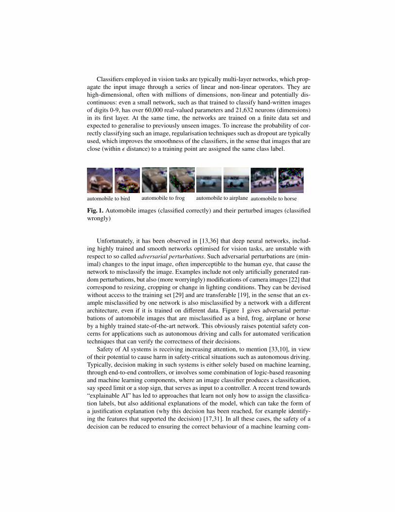
Deep neural networks have achieved impressive experimental results in image classifi-cation, matching the cognitive ability of humans [23] in complex tasks with thousandsof classes. Many applications are envisaged, including their use as perception modulesand end-to-end controllers for self-driving cars [15]. Let Rn be a vector space of images(points) that we wish to classify and assume that f : Rn → C, where C is a (finite) set ofclass labels, models the human perception capability, then a neural network classifier isa function f (x) which approximates f (x) from M training examples {(xi, ci)}i=1,..,M . Forexample, a perception module of a self-driving car may input an image from a cameraand must correctly classify the type of object in its view, irrespective of aspects suchas the angle of its vision and image imperfections. Therefore, though they clearly in-clude imperfections, all four pairs of images in Figure 1 should arguably be classifiedas automobiles, since they appear so to a human eye.

? This work is supported by the EPSRC Programme Grant on Mobile Autonomy(EP/M019918/1). Part of this work was done while MK was visiting the Simons Institute forthe Theory of Computing.

arX

iv:1

610.

0694

0v3

[cs

.AI]

5 M

ay 2

017

Classifiers employed in vision tasks are typically multi-layer networks, which prop-agate the input image through a series of linear and non-linear operators. They arehigh-dimensional, often with millions of dimensions, non-linear and potentially dis-continuous: even a small network, such as that trained to classify hand-written imagesof digits 0-9, has over 60,000 real-valued parameters and 21,632 neurons (dimensions)in its first layer. At the same time, the networks are trained on a finite data set andexpected to generalise to previously unseen images. To increase the probability of cor-rectly classifying such an image, regularisation techniques such as dropout are typicallyused, which improves the smoothness of the classifiers, in the sense that images that areclose (within ε distance) to a training point are assigned the same class label.

automobile to bird automobile to frog automobile to airplane automobile to horse

Fig. 1. Automobile images (classified correctly) and their perturbed images (classifiedwrongly)

Unfortunately, it has been observed in [13,36] that deep neural networks, includ-ing highly trained and smooth networks optimised for vision tasks, are unstable withrespect to so called adversarial perturbations. Such adversarial perturbations are (min-imal) changes to the input image, often imperceptible to the human eye, that cause thenetwork to misclassify the image. Examples include not only artificially generated ran-dom perturbations, but also (more worryingly) modifications of camera images [22] thatcorrespond to resizing, cropping or change in lighting conditions. They can be devisedwithout access to the training set [29] and are transferable [19], in the sense that an ex-ample misclassified by one network is also misclassified by a network with a differentarchitecture, even if it is trained on different data. Figure 1 gives adversarial pertur-bations of automobile images that are misclassified as a bird, frog, airplane or horseby a highly trained state-of-the-art network. This obviously raises potential safety con-cerns for applications such as autonomous driving and calls for automated verificationtechniques that can verify the correctness of their decisions.

Safety of AI systems is receiving increasing attention, to mention [33,10], in viewof their potential to cause harm in safety-critical situations such as autonomous driving.Typically, decision making in such systems is either solely based on machine learning,through end-to-end controllers, or involves some combination of logic-based reasoningand machine learning components, where an image classifier produces a classification,say speed limit or a stop sign, that serves as input to a controller. A recent trend towards“explainable AI” has led to approaches that learn not only how to assign the classifica-tion labels, but also additional explanations of the model, which can take the form ofa justification explanation (why this decision has been reached, for example identify-ing the features that supported the decision) [17,31]. In all these cases, the safety of adecision can be reduced to ensuring the correct behaviour of a machine learning com-

ponent. However, safety assurance and verification methodologies for machine learningare little studied.

The main difficulty with image classification tasks, which play a critical role in per-ception modules of autonomous driving controllers, is that they do not have a formalspecification in the usual sense: ideally, the performance of a classifier should matchthe perception ability and class labels assigned by a human. Traditionally, the correct-ness of a neural network classifier is expressed in terms of risk [37], defined as theprobability of misclassification of a given image, weighted with respect to the inputdistribution µ of images. Similar (statistical) robustness properties of deep neural net-work classifiers, which compute the average minimum distance to a misclassificationand are independent of the data point, have been studied and can be estimated usingtools such as DeepFool [25] and cleverhans [27]. However, we are interested in thesafety of an individual decision, and to this end focus on the key property of the clas-sifier being invariant to perturbations at a given point. This notion is also known aspointwise robustness [18,12] or local adversarial robustness [21].

Contributions. In this paper we propose a general framework for automated verifi-cation of safety of classification decisions made by feed-forward deep neural networks.Although we work concretely with image classifiers, the techniques can be generalisedto other settings. For a given image x (a point in a vector space), we assume that thereis a (possibly infinite) region η around that point that incontrovertibly supports the de-cision, in the sense that all points in this region must have the same class. This region isspecified by the user and can be given as a small diameter, or the set of all points whosesalient features are of the same type. We next assume that there is a family of operations∆, which we call manipulations, that specify modifications to the image under which theclassification decision should remain invariant in the region η. Such manipulations canrepresent, for example, camera imprecisions, change of camera angle, or replacement ofa feature. We define a network decision to be safe for input x and region η with respectto the set of manipulations ∆ if applying the manipulations on x will not result in a classchange for η. We employ discretisation to enable a finite exhaustive search of the high-dimensional region η for adversarial misclassifications. The discretisation approach isjustified in the case of image classifiers since they are typically represented as vectors ofdiscrete pixels (vectors of 8 bit RGB colours). To achieve scalability, we propagate theanalysis layer by layer, mapping the region and manipulations to the deeper layers. Weshow that this propagation is sound, and is complete under the additional assumption ofminimality of manipulations, which holds in discretised settings. In contrast to existingapproaches [36,28], our framework can guarantee that a misclassification is found if itexists. Since we reduce verification to a search for adversarial examples, we can achievesafety verification (if no misclassifications are found for all layers) or falsification (inwhich case the adversarial examples can be used to fine-tune the network or shown to ahuman tester).

We implement the techniques using Z3 [8] in a tool called DLV (Deep Learning Ver-ification) [2] and evaluate them on state-of-the-art networks, including regularised anddeep learning networks. This includes image classification networks trained for clas-sifying hand-written images of digits 0-9 (MNIST), 10 classes of small colour images(CIFAR10), 43 classes of the German Traffic Sign Recognition Benchmark (GTSRB)

[35] and 1000 classes of colour images used for the well-known imageNet large-scalevisual recognition challenge (ILSVRC) [4]. We also perform a comparison of the DLVfalsification functionality on the MNIST dataset against the methods of [36] and [28],focusing on the search strategies and statistical robustness estimation. The perturbedimages in Figure 1 are found automatically using our tool for the network trained onthe CIFAR10 dataset.

This invited paper is an extended and improved version of [20], where an extendedversion including appendices can also be found.

2 Background on Neural Networks

We consider feed-forward multi-layer neural networks [14], henceforth abbreviated asneural networks. Perceptrons (neurons) in a neural network are arranged in disjointlayers, with each perceptron in one layer connected to the next layer, but no connectionbetween perceptrons in the same layer. Each layer Lk of a network is associated withan nk-dimensional vector space DLk ⊆ R

nk , in which each dimension corresponds toa perceptron. We write Pk for the set of perceptrons in layer Lk and nk = |Pk | is thenumber of perceptrons (dimensions) in layer Lk.

Formally, a (feed-forward and deep) neural network N is a tuple (L,T, Φ), whereL = {Lk | k ∈ {0, ..., n}} is a set of layers such that layer L0 is the input layer and Ln

is the output layer, T ⊆ L × L is a set of sequential connections between layers suchthat, except for the input and output layers, each layer has an incoming connection andan outgoing connection, and Φ = {φk | k ∈ {1, ..., n}} is a set of activation functionsφk : DLk−1 → DLk , one for each non-input layer. Layers other than input and outputlayers are called the hidden layers.

The network is fed an input x (point in DL0 ) through its input layer, which is thenpropagated through the layers by successive application of the activation functions. Anactivation for point x in layer k is the value of the corresponding function, denotedαx,k = φk(φk−1(...φ1(x))) ∈ DLk , where αx,0 = x. For perceptron p ∈ Pk we writeαx,k(p) for the value of its activation on input x. For every activation αx,k and layerk′ < k, we define Prek′ (αx,k) = {αy,k′ ∈ DLk′ | αy,k = αx,k} to be the set of activations inlayer k′ whose corresponding activation in layer Lk is αx,k. The classification decisionis made based on the activations in the output layer by, e.g., assigning to x the classarg maxp∈Pn αx,n(p). For simplicity, we use αx,n to denote the class assigned to input x,and thus αx,n = αy,n expresses that two inputs x and y have the same class.

The neural network classifier N represents a function f (x) which approximatesf (x) : DL0 → C, a function that models the human perception capability in labelling im-ages with labels from C, from M training examples {(xi, ci)}i=1,..,M . Image classificationnetworks, for example convolutional networks, may contain many layers, which canbe non-linear, and work in high dimensions, which for the image classification prob-lems can be of the order of millions. Digital images are represented as 3D tensors ofpixels (width, height and depth, the latter to represent colour), where each pixel is a dis-crete value in the range 0..255. The training process determines real values for weightsused as filters that are convolved with the activation functions. Since it is difficult toapproximate f with few samples in the sparsely populated high-dimensional space, to

increase the probability of classifying correctly a previously unseen image, various reg-ularisation techniques such as dropout are employed. They improve the smoothness ofthe classifier, in the sense that points that are ε-close to a training point (potentiallyinfinitely many of them) classify the same.

In this paper, we work with the code of the network and its trained weights.

3 Safety Analysis of Classification Decisions

In this section we define our notion of safety of classification decisions for a neural net-work, based on the concept of a manipulation of an image, essentially perturbations thata human observer would classify the same as the original image. Safety is defined foran individual classification decision and is parameterised by the class of manipulationsand a neighbouring region around a given image. To ensure finiteness of the search ofthe region for adversarial misclassifications, we introduce so called “ladders”, nonde-terministically branching and iterated application of successive manipulations, and statethe conditions under which the search is exhaustive.

Safety and Robustness Our method assumes the existence of a (possibly infinite)region η around a data point (image) x such that all points in the region are indistin-guishable by a human, and therefore have the same true class. This region is understoodas supporting the classification decision and can usually be inferred from the type ofthe classification problem. For simplicity, we identify such a region via its diameter dwith respect to some user-specified norm, which intuitively measures the closeness tothe point x. As defined in [18], a network f approximating human capability f is saidto be not robust at x if there exists a point y in the region η = {z ∈ DL0 | ||z − x|| ≤ d}of the input layer such that f (x) , f (y). The point y, at a minimal distance from x, isknown as an adversarial example. Our definition of safety for a classification decision(abbreviated safety at a point) follows he same intuition, except that we work layerby layer, and therefore will identify such a region ηk, a subspace of DLk , at each layerLk, for k ∈ {0, ..., n}, and successively refine the regions through the deeper layers. Wejustify this choice based on the observation [11,23,24] that deep neural networks arethought to compute progressively more powerful invariants as the depth increases. Inother words, they gradually transform images into a representation in which the classesare separable by a linear classifier.

Assumption 1 For each activation αx,k of point x in layer Lk, the region ηk(αx,k) con-tains activations that the human observer believes to be so close to αx,k that they shouldbe classified the same as x.

Intuitively, safety for network N at a point x means that the classification decision isrobust at x against perturbations within the region ηk(αx,k). Note that, while the pertur-bation is applied in layer Lk, the classification decision is based on the activation in theoutput layer Ln.

Definition 1. [General Safety] Let ηk(αx,k) be a region in layer Lk of a neural networkN such that αx,k ∈ ηk(αx,k). We say that N is safe for input x and region ηk(αx,k), writtenas N, ηk |= x, if for all activations αy,k in ηk(αx,k) we have αy,n = αx,n.

We remark that, unlike the notions of risk [37] and robustness of [18,12], we workwith safety for a specific point and do not account for the input distribution, but suchexpectation measures can be considered, see Section 6 for comparison.

Manipulations A key concept of our framework is the notion of a manipulation, anoperator that intuitively models image perturbations, for example bad angles, scratchesor weather conditions, the idea being that the classification decisions in a region of im-ages close to it should be invariant under such manipulations. The choice of the type ofmanipulation is dependent on the application and user-defined, reflecting knowledge ofthe classification problem to model perturbations that should or should not be allowed.Judicious choice of families of such manipulations and appropriate distance metrics isparticularly important. For simplicity, we work with operators δk : DLk → DLk over theactivations in the vector space of layer k, and consider the Euclidean (L2) and Manhattan(L1) norms to measure the distance between an image and its perturbation through δk,but the techniques generalise to other norms discussed in [18,19,12]. More specifically,applying a manipulation δk(αx,k) to an activation αx,k will result in another activationsuch that the values of some or all dimensions are changed. We therefore represent amanipulation as a hyper-rectangle, defined for two activations αx,k and αy,k of layer Lk

by rec(αx,k, αy,k) = ×p∈Pk [min(αx,k(p), αy,k(p)), max(αx,k(p), αy,k(p))]. The main chal-lenge for verification is the fact that the region ηk contains potentially an uncountablenumber of activations. Our approach relies on discretisation in order to enable a finiteexploration of the region to discover and/or rule out adversarial perturbations.

For an activation αx,k and a set ∆ of manipulations, we denote by rec(∆, αx,k) thepolyhedron which includes all hyper-rectangles that result from applying some manip-ulation in ∆ on αx,k, i.e., rec(∆, αx,k) =

⋃δ∈∆ rec(αx,k, δ(αx,k)). Let ∆k be the set of all

possible manipulations for layer Lk. To ensure region coverage, we define valid manip-ulation as follows.

Definition 2. Given an activation αx,k, a set of manipulations V(αx,k) ⊆ ∆k is valid ifαx,k is an interior point of rec(V(αx,k), αx,k), i.e., αx,k is in rec(V(αx,k), αx,k) and doesnot belong to the boundary of rec(V(αx,k), αx,k).

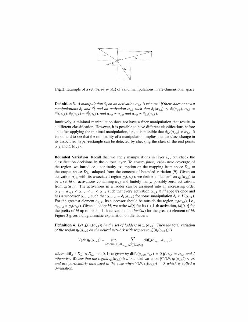
Figure 2 presents an example of valid manipulations in two-dimensional space: eacharrow represents a manipulation, each dashed box represents a (hyper-)rectangle of thecorresponding manipulation, and activation αx,k is an interior point of the space fromthe dashed boxes.

Since we work with discretised spaces, which is a reasonable assumption for im-ages, we introduce the notion of a minimal manipulation. If applying a minimal manip-ulation, it suffices to check for misclassification just at the end points, that is, αx,k andδk(αx,k). This allows an exhaustive, albeit impractical, exploration of the region in unitsteps.

A manipulation δ1k(αy,k) is finer than δ2

k(αx,k), written as δ1k(αy,k) ≤ δ2

k(αx,k), if anyactivation in the hyper-rectangle of the former is also in the hyper-rectangle of the latter.It is implied in this definition that αy,k is an activation in the hyper-rectangle of δ2

k(αx,k).Moreover, we write δk,k′ (αx,k) for φk′ (...φk+1(δk(αx,k))), representing the correspondingactivation in layer k′ ≥ k after applying manipulation δk on the activation αx,k, whereδk,k(αx,k) = δk(αx,k).

�1�1

�2�2

�3�3

�4�4

↵x,k↵x,k

Fig. 2. Example of a set {δ1, δ2, δ3, δ4} of valid manipulations in a 2-dimensional space

Definition 3. A manipulation δk on an activation αx,k is minimal if there does not existmanipulations δ1

k and δ2k and an activation αy,k such that δ1

k(αx,k) ≤ δk(αx,k), αy,k =

δ1k(αx,k), δk(αx,k) = δ2

k(αy,k), and αy,n , αx,n and αy,n , δk,n(αx,k).

Intuitively, a minimal manipulation does not have a finer manipulation that results ina different classification. However, it is possible to have different classifications beforeand after applying the minimal manipulation, i.e., it is possible that δk,n(αx,k) , αx,n. Itis not hard to see that the minimality of a manipulation implies that the class change inits associated hyper-rectangle can be detected by checking the class of the end pointsαx,k and δk(αx,k).

Bounded Variation Recall that we apply manipulations in layer Lk, but check theclassification decisions in the output layer. To ensure finite, exhaustive coverage ofthe region, we introduce a continuity assumption on the mapping from space DLk tothe output space DLn , adapted from the concept of bounded variation [9]. Given anactivation αx,k with its associated region ηk(αx,k), we define a “ladder” on ηk(αx,k) tobe a set ld of activations containing αx,k and finitely many, possibly zero, activationsfrom ηk(αx,k). The activations in a ladder can be arranged into an increasing orderαx,k = αx0,k < αx1,k < ... < αx j,k such that every activation αxt ,k ∈ ld appears once andhas a successor αxt+1,k such that αxt+1,k = δk(αxt ,k) for some manipulation δk ∈ V(αxt ,k).For the greatest element αx j,k, its successor should be outside the region ηk(αx,k), i.e.,αx j+1,k < ηk(αx,k). Given a ladder ld, we write ld(t) for its t + 1-th activation, ld[0..t] forthe prefix of ld up to the t + 1-th activation, and last(ld) for the greatest element of ld.Figure 3 gives a diagrammatic explanation on the ladders.

Definition 4. Let L(ηk(αx,k)) be the set of ladders in ηk(αx,k). Then the total variationof the region ηk(αx,k) on the neural network with respect to L(ηk(αx,k)) is

V(N; ηk(αx,k)) = supld∈L(ηk(αx,k))

∑αxt ,k∈ld\{last(ld)}

diffn(αxt ,n, αxt+1,n)

where diffn : DLn × DLn → {0, 1} is given by diffn(αx,n, αy,n) = 0 if αx,n = αy,n and 1otherwise. We say that the region ηk(αx,k) is a bounded variation if V(N; ηk(αx,k)) < ∞,and are particularly interested in the case when V(N; rk(αy,k)) = 0, which is called a0-variation.

�k�k

�k�k

�k�k

�k�k

�k�k

�k�k

↵x,k = ↵x0,k↵x,k = ↵x0,k↵x1,k↵x1,k

↵x2,k↵x2,k

↵xj ,k↵xj ,k

↵xj+1,k↵xj+1,k⌘k(↵x,k)⌘k(↵x,k)

Fig. 3. Examples of ladders in region ηk(αx,k). Starting from αx,k = αx0,k, the activationsαx1,k...αx j,k form a ladder such that each consecutive activation results from some validmanipulation δk applied to a previous activation, and the final activation αx j,k is outsidethe region ηk(αx,k).

The setL(ηk(αx,k)) is complete if, for any ladder ld ∈ L(ηk(αx,k)) of j+1 activations,any element ld(t) for 0 ≤ t ≤ j, and any manipulation δk ∈ V(ld(t)), there exists a ladderld′ ∈ L(ηk(αx,k)) such that ld′[0..t] = ld[0..t] and ld′(t + 1) = δk(ld(t)). Intuitively, acomplete ladder is a complete tree, on which each node represents an activation andeach branch of a node corresponds to a valid manipulation. From the root αx,k, everypath of the tree leading to a leaf is a ladder. Moreover, the set L(ηk(αx,k)) is covering ifthe polyhedra of all activations in it cover the region ηk(αx,k), i.e.,

ηk(αx,k) ⊆⋃

ld∈L(ηk(αx,k))

⋃αxt ,k∈ld\{last(ld)}

rec(V(αxt ,k), αxt ,k). (1)

Based on the above, we have the following definition of safety with respect to a setof manipulations. Intuitively, we iteratively and nondeterministically apply manipula-tions to explore the region ηk(αx,k), and safety means that no class change is observedby successive application of such manipulations.

Definition 5. [Safety wrt Manipulations] Given a neural network N, an input x and aset ∆k of manipulations, we say that N is safe for input x with respect to the region ηk

and manipulations ∆k, written as N, ηk, ∆k |= x, if the region ηk(αx,k) is a 0-variation forthe set L(ηk(αx,k)) of its ladders, which is complete and covering.

It is straightforward to note that general safety in the sense of Definition 1 impliessafety wrt manipulations, in the sense of Definition 5.

Theorem 1. Given a neural network N, an input x, and a region ηk, we have thatN, ηk |= x implies N, ηk, ∆k |= x for any set of manipulations ∆k.

In the opposite direction, we require the minimality assumption on manipulations.

Theorem 2. Given a neural network N, an input x, a region ηk(αx,k) and a set ∆k ofmanipulations, we have that N, ηk, ∆k |= x implies N, ηk |= x if the manipulations in ∆k

are minimal.

Theorem 2 means that, under the minimality assumption over the manipulations, anexhaustive search through the complete and covering ladder tree from L(ηk(αx,k)) canfind adversarial examples, if any, and enable us to conclude that the network is safeat a given point if none are found. Though computing minimal manipulations is notpractical, in discrete spaces by iterating over increasingly refined manipulations we areable to rule out the existence of adversarial examples in the region. This contrasts withpartial exploration according to, e.g., [25,12]; for comparison see Section 7.

4 The Verification Framework

In this section we propose a novel framework for automated verification of safety ofclassification decisions, which is based on search for an adversarial misclassificationwithin a given region. The key distinctive distinctive features of our framework com-pared to existing work are: a guarantee that a misclassification is found if it exists; thepropagation of the analysis layer by layer; and working with hidden layers, in addi-tion to input and output layers. Since we reduce verification to a search for adversarialexamples, we can achieve safety verification (if no misclassifications are found for alllayers) or falsification (in which case the adversarial examples can be used to fine-tunethe network or shown to a human tester).

4.1 Layer-by-Layer Analysis

We first consider how to propagate the analysis layer by layer, which will involve refin-ing manipulations through the hidden layers. To facilitate such analysis, in addition tothe activation function φk : DLk−1 → DLk we also require a mapping ψk : DLk → DLk−1

in the opposite direction, to represent how a manipulated activation of layer Lk affectsthe activations of layer Lk−1. We can simply take ψk as the inverse function of φk. Inorder to propagate safety of regions ηk(αx,k) at a point x into deeper layers, we assumethe existence of functions ηk that map activations to regions, and impose the followingrestrictions on the functions φk and ψk, shown diagrammatically in Figure 4.

Definition 6. The functions {η0, η1, ..., ηn} and {ψ1, ..., ψn} mapping activations to re-gions are such that

1. ηk(αx,k) ⊆ DLk , for k = 0, ..., n,2. αx,k ∈ ηk(αx,k), for k = 0, ..., n, and3. ηk−1(αi,k−1) ⊆ ψk(ηk(αx,k)) for all k = 1, ..., n.

Intuitively, the first two conditions state that each function ηk assigns a region aroundthe activation αx,k, and the last condition that mapping the region ηk from layer Lk to

Lk−1 via ψk should cover the region ηk−1. The aim is to compute functions ηk+1, ..., ηn

based on ηk and the neural network.The size and complexity of a deep neural network generally means that determining

whether a given set ∆k of manipulations is minimal is intractable. To partially counterthis, we define a refinement relation between safety wrt manipulations for consecutivelayers in the sense that N, ηk, ∆k |= x is a refinement of N, ηk−1, ∆k−1 |= x if all ma-nipulations δk−1 in ∆k−1 are refined by a sequence of manipulations δk from the set ∆k.Therefore, although we cannot theoretically confirm the minimality of ∆k, they are re-fined layer by layer and, in discrete settings, this process can be bounded from belowby the unit step. Moreover, we can work gradually from a specific layer inwards untilan adversarial example is found, finishing processing when reaching the output layer.

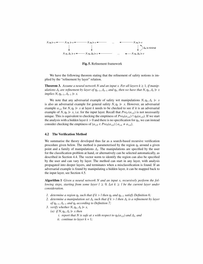
The refinement framework is given in Figure 5. The arrows represent the implication

⌘0(↵x,0)⌘0(↵x,0)

↵x,0↵x,0

↵x,k↵x,k

⌘k(↵x,k)⌘k(↵x,k)

↵x,n↵x,n

⌘n(↵x,n)⌘n(↵x,n)

layer 0 layer k layer n

⌘k�1(↵x,k�1)⌘k�1(↵x,k�1)

↵x,k�1↵x,k�1

k k

layer k-1

DL0DL0 DLk�1DLk�1

DLkDLk DLnDLn

�k�k

Fig. 4. Layer by layer analysis according to Definition 6

relations between the safety notions and are labelled with conditions if needed. Thegoal of the refinements is to find a chain of implications to justify N, η0 |= x. Thefact that N, ηk |= x implies N, ηk−1 |= x is due to the constraints in Definition 6 whenψk = φ−1

k . The fact that N, ηk |= x implies N, ηk, ∆k |= x follows from Theorem 1. Theimplication from N, ηk, ∆k |= x to N, ηk |= x under the condition that ∆k is minimal isdue to Theorem 2.

We now define the notion of refinability of manipulations between layers. Intu-itively, a manipulation in layer Lk−1 is refinable in layer Lk if there exists a sequence ofmanipulations in layer Lk that implements the manipulation in layer Lk−1.

Definition 7. A manipulation δk−1(αy,k−1) is refinable in layer Lk if there exist activa-tions αx0,k, ..., αx j,k ∈ DLk and valid manipulations δ1

k ∈ V(αx0,k), ..., δ jk ∈ V(αx j−1,k) such

that αy,k = αx0,k, δk−1,k(αy,k−1) = αx j,k, and αxt ,k = δtk(αxt−1,k) for 1 ≤ t ≤ j. Given a

neural network N and an input x, the manipulations ∆k are a refinement by layer ofηk−1, ∆k−1 and ηk if, for all αy,k−1 ∈ ηk−1(αz,k−1), all its valid manipulations δk−1(αy,k−1)are refinable in layer Lk.

N, ⌘0 |= xN, ⌘0 |= x N, ⌘1 |= xN, ⌘1 |= x N, ⌘2 |= xN, ⌘2 |= x N, ⌘k |= xN, ⌘k |= x

N, ⌘1,�1 |= xN, ⌘1,�1 |= x N, ⌘2,�2 |= xN, ⌘2,�2 |= x N, ⌘k,�k |= xN, ⌘k,�k |= x

�k�k is minimal

…

…

Fig. 5. Refinement framework

We have the following theorem stating that the refinement of safety notions is im-plied by the “refinement by layer” relation.

Theorem 3. Assume a neural network N and an input x. For all layers k ≥ 1, if manip-ulations ∆k are refinement by layer of ηk−1, ∆k−1 and ηk, then we have that N, ηk, ∆k |= ximplies N, ηk−1, ∆k−1 |= x.

We note that any adversarial example of safety wrt manipulations N, ηk, ∆k |= xis also an adversarial example for general safety N, ηk |= x. However, an adversarialexample αx,k for N, ηk |= x at layer k needs to be checked to see if it is an adversarialexample of N, η0 |= x, i.e. for the input layer. Recall that Prek′ (αx,k) is not necessarilyunique. This is equivalent to checking the emptiness of Pre0(αx,k)∩ η0(αx,0). If we startthe analysis with a hidden layer k > 0 and there is no specification for η0, we can insteadconsider checking the emptiness of {αy,0 ∈ Pre0(αx,k) | αy,n , αx,n}.

4.2 The Verification Method

We summarise the theory developed thus far as a search-based recursive verificationprocedure given below. The method is parameterised by the region ηk around a givenpoint and a family of manipulations ∆k. The manipulations are specified by the userfor the classification problem at hand, or alternatively can be selected automatically, asdescribed in Section 4.4. The vector norm to identify the region can also be specifiedby the user and can vary by layer. The method can start in any layer, with analysispropagated into deeper layers, and terminates when a misclassification is found. If anadversarial example is found by manipulating a hidden layer, it can be mapped back tothe input layer, see Section 4.5.

Algorithm 1 Given a neural network N and an input x, recursively perform the fol-lowing steps, starting from some layer l ≥ 0. Let k ≥ l be the current layer underconsideration.

1. determine a region ηk such that if k > l then ηk and ηk−1 satisfy Definition 6;2. determine a manipulation set ∆k such that if k > l then ∆k is a refinement by layer

of ηk−1, ∆k−1 and ηk according to Definition 7;3. verify whether N, ηk, ∆k |= x,

(a) if N, ηk, ∆k |= x theni. report that N is safe at x with respect to ηk(αx,k) and ∆k, and

ii. continue to layer k + 1;

(b) if N, ηk, ∆k 6|= x, then report an adversarial example.

We implement Algorithm 1 by utilising satisfiability modulo theory (SMT) solvers.The SMT problem is a decision problem for logical formulas with respect to combina-tions of background theories expressed in classical first-order logic with equality. Forchecking refinement by layer, we use the theory of linear real arithmetic with existen-tial and universal quantifiers, and for verification within a layer (0-variation) we use thesame theory but without universal quantification. The details of the encoding and the ap-proach taken to compute the regions and manipulations are included in Section 4.4. Toenable practical verification of deep neural networks, we employ a number of heuristicsdescribed in the remainder of this section.

4.3 Feature Decomposition and Discovery

While Theorem 1 and 2 provide a finite way to verify safety of neural network clas-sification decisions, the high-dimensionality of the region ηk(αx,k) can make any com-putational approach impractical. We therefore use the concept of a feature to parti-tion the region ηk(αx,k) into a set of features, and exploit their independence and low-dimensionality. This allows us to work with state-of-the-art networks that have hun-dreds, and even thousands, of dimensions.

Intuitively, a feature defines for each point in the high-dimensional space DLk themost explicit salient feature it has, e.g., the red-coloured frame of a street sign in Fig-ure 10. Formally, for each layer Lk, a feature function fk : DLk → P(DLk ) assigns a smallregion for each activation αx,k in the space DLk , where P(DLk ) is the set of subspaces ofDLk . The region fk(αx,k) may have lower dimension than that of Dk. It has been argued,in e.g. [16] for natural images, that natural data, for example natural images and sound,forms a high-dimensional manifold, which embeds tangled manifolds to represent theirfeatures. Feature manifolds usually have lower dimension than the data manifold, and aclassification algorithm is to separate a set of tangled manifolds. By assuming that theappearance of features is independent, we can manipulate them one by one regardlessof the manipulation order, and thus reduce the problem of size O(2d1+...+dm ) into a set ofsmaller problems of size O(2d1 ), ...,O(2dm ).

The analysis of activations in hidden layers, as performed by our method, providesan opportunity to discover the features automatically. Moreover, defining the featurefk on each activation as a single region corresponding to a specific feature is withoutloss of generality: although an activation may include multiple features, the indepen-dence relation between features suggests the existence of a total relation between thesefeatures. The function fk essentially defines for each activation one particular feature,subject to certain criteria such as explicit knowledge, but features can also be exploredin parallel.

Every feature fk(αy,k) is identified by a pre-specified number dimsk, f of dimensions.Let dimsk( fk(αy,k)) be the set of dimensions selected according to some heuristic. Thenwe have that

fk(αy,k)(p) =

{ηk(αx,k)(p), if p ∈ dimsk( fk(αy,k))[αy,k(p), αy,k(p)] otherwise. (2)

Moreover, we need a set of features to partition the region ηk(αx,k) as follows.

Definition 8. A set { f1, ..., fm} of regions is a partition of ηk(αx,k), written as π(ηk(αx,k)),if dimsk, f ( fi) ∩ dimsk, f ( f j) = ∅ for i, j ∈ {1, ...,m} and ηk(αx,k) = ×m

i=1 fi.

Given such a partition π(ηk(αx,k)), we define a function acts(x, k) by

acts(x, k) = {αy,k ∈ x | x ∈ π(ηk(αx,k))} (3)

which contains one point for each feature. Then, we reduce the checking of 0-variationof a region ηk(αx,k) to the following problems:

– checking whether the points in acts(x, k) have the same class as αx,k, and– checking the 0-variation of all features in π(ηk(αx,k)).

In the above procedure, the checking of points in acts(x, k) can be conducted ei-ther by following a pre-specified sequential order (single-path search) or by exhaus-tively searching all possible orders (multi-path search). In Section 5 we demonstratethat single-path search according to the prominence of features can enable us to findadversarial examples, while multi-path search may find other examples whose distanceto the original input image is smaller.

4.4 Selection of Regions and Manipulations

The procedure summarised in Algorithm 1 is typically invoked for a given image in theinput layer, but, providing insight about hidden layers is available, it can start from anylayer Ll in the network. The selection of regions can be automated, as described below.

For the first layer to be considered, i.e., k = l, the region ηk(αx,k) is defined by firstselecting the subset of dimsk dimensions from Pk whose activation values are furthestaway from the average activation value of the layer1. Intuitively, the knowledge repre-sented by these activations is more explicit than the knowledge represented by the otherdimensions, and manipulations over more explicit knowledge are more likely to resultin a class change. Let avgk = (

∑p∈Pk

αx,k(p))/nk be the average activation value of layerLk. We let dimsk(ηk(αx,k)) be the first dimsk dimensions p ∈ Pk with the greatest values|αx,k(p) − avg| among all dimensions, and then define

ηk(αx,k) = ×p∈dimsk(ηk(αx,k))[αx,k(p) − sp ∗ mp, αx,k(p) + sp ∗ mp] (4)

i.e., a dimsk-polytope containing the activation αx,k, where sp represents a small spanand mp represents the number of such spans. Let Vk = {sp,mp | p ∈ dimsk(ηk(αx,k))} bea set of variables.

Let d be a function mapping from dimsk(ηk(αx,k)) to {−1, 0,+1} such that {d(p) ,0 | p ∈ dimsk(ηk(αx,k))} , ∅, and D(dimsk(ηk(αx,k))) be the set of such functions. Let amanipulation δd

k be

δdk (αy,k)(p) =

αy,k(p) − sp if d(p) = −1αy,k(p) if d(p) = 0αy,k(p) + sp if d(p) = +1

(5)

1 We also considered other approaches, including computing derivatives up to several layers, butfor the experiments we conduct they are less effective.

for activation αy,k ∈ ηk(αx,k). That is, each manipulation changes a subset of the dimen-sions by the span sp, according to the directions given in d. The set ∆k is defined by col-lecting the set of all such manipulations. Based on this, we can define a set L(ηk(αx,k))of ladders, which is complete and covering.

Determining the region ηk according to ηk−1 Given ηk−1(αx,k−1) and the functions φk

and ψk, we can automatically determine a region ηk(αx,k) satisfying Definition 6 usingthe following approach. According to the function φk, the activation value αx,k(p) ofperceptron p ∈ Pk is computed from activation values of a subset of perceptrons inPk−1. We let Vars(p) ⊆ Pk−1 be such a set of perceptrons. The selection of dimensionsin dimsk(ηk(αx,k)) depends on dimsk−1(ηk−1(αx,k−1)) and φk, by requiring that, for everyp′ ∈ dimsk−1(ηk−1(αx,k−1)), there is at least one dimension p ∈ dimsk(ηk(αx,k)) such thatp′ ∈ Vars(p). We let

dimsk(ηk(αx,k)) = {arg maxp∈Pk

{ |αx,k(p)−avgk | | p′ ∈ Vars(p)} | p′ ∈ dimsk−1(ηk−1(αx,k−1))}

(6)Therefore, the restriction of Definition 6 can be expressed with the following formula:

∀αy,k−1 ∈ ηk(αx,k−1) : αy,k−1 ∈ ψk(ηk(αx,k)). (7)

We omit the details of rewriting αy,k−1 ∈ ηk(αx,k−1) and αy,k−1 ∈ ψk(ηk(αx,k)) intoBoolean expressions, which follow from standard techniques. Note that this expres-sion includes variables in Vk,Vk−1 and αy,k−1. The variables in Vk−1 are fixed for a givenηk−1(αx,k−1). Because such a region ηk(αx,k) always exists, a simple iterative procedurecan be invoked to gradually increase the size of the region represented with variables inVk to eventually satisfy the expression.

Determining the manipulation set ∆k according to ηk(αx,k), ηk−1(αx,k−1), and ∆k−1The values of the variables Vk obtained from the satisfiability of Eqn (7) yield a defini-tion of manipulations using Eqn (5). However, the obtained values for span variables sp

do not necessarily satisfy the “refinement by layer” relation as defined in Definition 7.Therefore, we need to adapt the values for the variables Vk while, at the same time,retaining the region ηk(αx,k). To do so, we could rewrite the constraint in Definition 7into a formula, which can then be solved by an SMT solver. But, in practice, we noticethat such precise computations easily lead to overly small spans sp, which in turn resultin an unacceptable amount of computation needed to verify the relation N, ηk, ∆k |= x.

To reduce computational cost, we work with a weaker “refinable in layer Lk” notion,parameterised with respect to precision ε. Given two activations αy,k and αm,k, we usedist(αy,k, αm,k) to represent their distance.

Definition 9. A manipulation δk−1(αy,k−1) is refinable in layer Lk with precision ε > 0if there exists a sequence of activations αx0,k, ..., αx j,k ∈ DLk and valid manipulationsδ1

k ∈ V(αx0,k), ..., δdk ∈ V(αx j−1,k) such that αy,k = αx0,k, δk−1,k(αy,k−1) ∈ rec(αx j−1,k, αx j,k),

dist(αx j−1,k, αx j,k) ≤ ε, and αxt ,k = δtk(αxt−1,k) for 1 ≤ t ≤ j. Given a neural network N

and an input x, the manipulations ∆k are a refinement by layer of ηk, ηk−1, ∆k−1 with

precision ε if, for all αy,k−1 ∈ ηk−1(αx,k−1), all its legal manipulations δk−1(αy,k−1) arerefinable in layer Lk with precision ε.

Comparing with Definition 7, the above definition replaces δk−1,k(αy,k−1) = αx j,k

with δk−1,k(αy,k−1) ∈ rec(αx j−1,k, αx j,k) and dist(αx j−1,k, αx j,k) ≤ ε. Intuitively, instead ofrequiring a manipulation to reach the activation δk−1,k(αy,k−1) precisely, this definitionallows for each δk−1,k(αy,k−1) to be within the hyper-rectangle rec(αx j−1,k, αx j,k). To findsuitable values for Vk according to the approximate “refinement-by-layer” relation, weuse a variable h to represent the maximal number of manipulations of layer Lk used toexpress a manipulation in layer k − 1. The value of h (and variables sp and np in Vk)are automatically adapted to ensure the satisfiability of the following formula, whichexpresses the constraints of Definition 9:

∀αy,k−1 ∈ ηk(αx,k−1)∀d ∈ D(dimsk(ηk(αx,k−1)))∀δdk−1 ∈ Vk−1(αy,k−1)

∃αy0,k, ..., αyh,k ∈ ηk(αx,k) : αy0,k = αy,k ∧∧h−1

t=0 αyt+1,k = δdk (αyt ,k)∧∨h−1

t=0 (δdk−1,k(αy,k) ∈ rec(αyt ,k, αyt+1,k) ∧ dist(αyt ,k, αyt+1,k) ≤ ε).

(8)

It is noted that sp and mp for p ∈ dimsk(ηk(αx,k)) are employed when expressing δdk .

The manipulation δdk is obtained from δd

k−1 by considering the corresponding relationbetween dimensions in dimsk(ηk(αx,k)) and dimsk−1(ηk−1(αx,k−1)).

Adversarial examples shown in Figures 8, 9, and 10 were found using single-pathsearch and automatic selection of regions and manipulations.

4.5 Mapping Back to Input Layer

When manipulating the hidden layers, we may need to map back an activation in layerk to the input layer to obtain an input image that resulted in misclassification, whichinvolves computation of Pre0(αy,k) described next. To check the 0-variation of a regionηk(αx,k), we need to compute diffn(αx,n, αy,n) for many points αy,x in ηk(αx,k), wherediffn : DLn ×DLn → {0, 1} is given by diffn(αx,n, αy,n) = 0 if αx,n = αy,n and 1 otherwise.Because αx,n is known, we only need to compute αy,n. We can compute αy,n by findinga point αy,0 ∈ Pre0(αy,k) and then using the neural network to predict the value αy,n. Itshould be noted that, although Pre0(αy,k) may include more than one point, all pointshave the same class, so any point in Pre0(αy,k) is sufficient for our purpose.

To compute αy,0 from αy,k, we use functions ψk, ψk−1, ..., ψ1 and compute pointsαy,k−1, αy,k−2, ..., αy,0 such that

αy, j−1 = ψ j(αy, j) ∧ αy, j−1 ∈ η j−1(αx, j−1)

for 1 ≤ j ≤ k. The computation relies on an SMT solver to encode the functionsψk, ψk−1, ..., ψ1 if they are piecewise linear functions, and by taking the correspondinginverse functions directly if they are sigmoid functions. It is possible that, for some1 ≤ j ≤ k, no point can be found by SMT solver, which means that the point αy,k doesnot have any corresponding point in the input layer. We can safely discard these points.The maxpooling function ψ j selects from every m ∗m dimensions the maximal elementfor some m > 0. The computation of the maxpooling layer ψ j−1 is combined with thecomputation of the next layer ψ j, that is, finding αy, j−2 with the following expression

∃αx, j−1 : αy, j−2 = ψ j−1(ψ j(αy, j)) ∧ αy, j−1 ∈ η j−1(αx, j−1) ∧ αy, j−2 ∈ η j−2(αx, j−2)

This is to ensure that in the expression αy, j−2 = ψ j−1(ψ j(αy, j)) we can reuse m ∗ m − 1elements in αx, j−2 and only need to replace the maximal element.

Figures 8, 9, and 10 show images obtained by mapping back from the first hiddenlayer to the input layer.

5 Experimental Results

The proposed framework has been implemented as a software tool called DLV (DeepLearning Verification) [2] written in Python, see Appendix of [20] for details of inputparameters and how to use the tool. The SMT solver we employ is Z3 [8], which hasPython APIs. The neural networks are built from a widely-used neural networks libraryKeras [3] with a deep learning package Theano [6] as its backend.

We validate DLV on a set of experiments performed for neural networks trained forclassification based on a predefined multi-dimensional surface (small size networks),as well as image classification (medium size networks). These networks respectivelyuse two representative types of layers: fully connected layers and convolutional layers.They may also use other types of layers, e.g., the ReLU layer, the pooling layer, thezero-padding layer, and the dropout layer. The first three demonstrate the single-pathsearch functionality on the Euclidean (L2) norm, whereas the fourth (GTSRB) multi-path search for the L1 and L2 norms.

The experiments are conducted on a MacBook Pro laptop, with 2.7 GHz Intel Corei5 CPU and 8 GB memory.

Two-Dimensional Point Classification Network To demonstrate exhaustive verifica-tion facilitated by our framework, we consider a neural network trained for classifyingpoints above and below a two-dimensional curve shown in red in Figure 6 and Figure 7.The network has three fully-connected hidden layers with the ReLU activation func-tion. The input layer has two perceptrons, every hidden layer has 20 perceptrons, andthe output layer has two perceptrons. The network is trained with 5,000 points sampledfrom the provided two-dimensional space, and has an accuracy of more than 99%.

For a given input x = (3.59, 1.11), we start from the input layer and define a regionaround this point by taking unit steps in both directions

η0(αx,0) = [3.59− 1.0, 3.59 + 1.0]× [1.11− 1.0, 1.11 + 1.0] = [2.59, 4.59]× [0.11, 2.11]

The manipulation set ∆0 is shown in Figure 6: there are 9 points, of which the point inthe middle represents the activation αx,0 and the other 8 points represent the activationsresulting from applying one of the manipulations in ∆0 on αx,0. Note that, although thereare class changes in the region η0(αx,0), the manipulation set ∆0 is not able to detect suchchanges. Therefore, we have that N, η0, ∆0 |= x.

Now consider layer k = 1. To obtain the region η1(αx,1), the tool selects two dimen-sions p1,17, p1,19 ∈ P1 in layer L1 with indices 17 and 19 and computes

η1(αx,1) = [αx,1(p1,17) − 3.6, αx,1(p1,17) + 3.6] × [αx,1(p1,19) − 3.52, αx,1(p1,19) + 3.52]

The manipulation set ∆1, after mapping back to the input layer with function ψ1, is givenas Figure 7. Note that η1 and η0 satisfy Definition 6, and ∆1 is a refinement by layer of

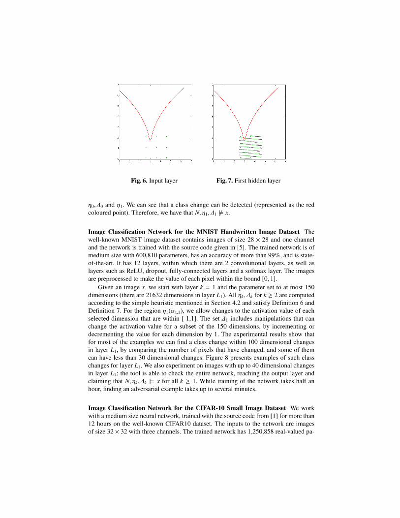
Fig. 6. Input layer Fig. 7. First hidden layer

η0, ∆0 and η1. We can see that a class change can be detected (represented as the redcoloured point). Therefore, we have that N, η1, ∆1 6|= x.

Image Classification Network for the MNIST Handwritten Image Dataset Thewell-known MNIST image dataset contains images of size 28 × 28 and one channeland the network is trained with the source code given in [5]. The trained network is ofmedium size with 600,810 parameters, has an accuracy of more than 99%, and is state-of-the-art. It has 12 layers, within which there are 2 convolutional layers, as well aslayers such as ReLU, dropout, fully-connected layers and a softmax layer. The imagesare preprocessed to make the value of each pixel within the bound [0, 1].

Given an image x, we start with layer k = 1 and the parameter set to at most 150dimensions (there are 21632 dimensions in layer L1). All ηk, ∆k for k ≥ 2 are computedaccording to the simple heuristic mentioned in Section 4.2 and satisfy Definition 6 andDefinition 7. For the region η1(αx,1), we allow changes to the activation value of eachselected dimension that are within [-1,1]. The set ∆1 includes manipulations that canchange the activation value for a subset of the 150 dimensions, by incrementing ordecrementing the value for each dimension by 1. The experimental results show thatfor most of the examples we can find a class change within 100 dimensional changesin layer L1, by comparing the number of pixels that have changed, and some of themcan have less than 30 dimensional changes. Figure 8 presents examples of such classchanges for layer L1. We also experiment on images with up to 40 dimensional changesin layer L1; the tool is able to check the entire network, reaching the output layer andclaiming that N, ηk, ∆k |= x for all k ≥ 1. While training of the network takes half anhour, finding an adversarial example takes up to several minutes.

Image Classification Network for the CIFAR-10 Small Image Dataset We workwith a medium size neural network, trained with the source code from [1] for more than12 hours on the well-known CIFAR10 dataset. The inputs to the network are imagesof size 32 × 32 with three channels. The trained network has 1,250,858 real-valued pa-

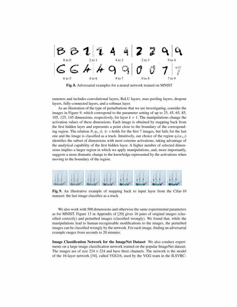
8 to 0 2 to 1 4 to 2 2 to 3 9 to 4

6 to 5 4 to 6 9 to 7 0 to 8 7 to 9

Fig. 8. Adversarial examples for a neural network trained on MNIST

rameters and includes convolutional layers, ReLU layers, max-pooling layers, dropoutlayers, fully-connected layers, and a softmax layer.

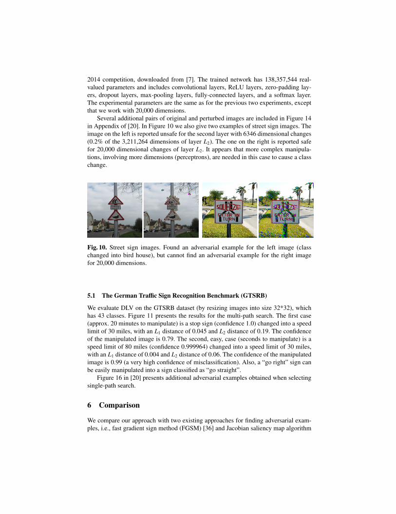
As an illustration of the type of perturbations that we are investigating, consider theimages in Figure 9, which correspond to the parameter setting of up to 25, 45, 65, 85,105, 125, 145 dimensions, respectively, for layer k = 1. The manipulations change theactivation values of these dimensions. Each image is obtained by mapping back fromthe first hidden layer and represents a point close to the boundary of the correspond-ing region. The relation N, η1, ∆1 |= x holds for the first 7 images, but fails for the lastone and the image is classified as a truck. Intuitively, our choice of the region η1(αx,1)identifies the subset of dimensions with most extreme activations, taking advantage ofthe analytical capability of the first hidden layer. A higher number of selected dimen-sions implies a larger region in which we apply manipulations, and, more importantly,suggests a more dramatic change to the knowledge represented by the activations whenmoving to the boundary of the region.

Fig. 9. An illustrative example of mapping back to input layer from the Cifar-10mataset: the last image classifies as a truck.

We also work with 500 dimensions and otherwise the same experimental parametersas for MNIST. Figure 13 in Appendix of [20] gives 16 pairs of original images (clas-sified correctly) and perturbed images (classified wrongly). We found that, while themanipulations lead to human-recognisable modifications to the images, the perturbedimages can be classified wrongly by the network. For each image, finding an adversarialexample ranges from seconds to 20 minutes.

Image Classification Network for the ImageNet Dataset We also conduct experi-ments on a large image classification network trained on the popular ImageNet dataset.The images are of size 224 × 224 and have three channels. The network is the modelof the 16-layer network [34], called VGG16, used by the VGG team in the ILSVRC-

2014 competition, downloaded from [7]. The trained network has 138,357,544 real-valued parameters and includes convolutional layers, ReLU layers, zero-padding lay-ers, dropout layers, max-pooling layers, fully-connected layers, and a softmax layer.The experimental parameters are the same as for the previous two experiments, exceptthat we work with 20,000 dimensions.

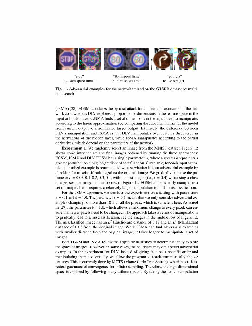
Several additional pairs of original and perturbed images are included in Figure 14in Appendix of [20]. In Figure 10 we also give two examples of street sign images. Theimage on the left is reported unsafe for the second layer with 6346 dimensional changes(0.2% of the 3,211,264 dimensions of layer L2). The one on the right is reported safefor 20,000 dimensional changes of layer L2. It appears that more complex manipula-tions, involving more dimensions (perceptrons), are needed in this case to cause a classchange.

Fig. 10. Street sign images. Found an adversarial example for the left image (classchanged into bird house), but cannot find an adversarial example for the right imagefor 20,000 dimensions.

5.1 The German Traffic Sign Recognition Benchmark (GTSRB)

We evaluate DLV on the GTSRB dataset (by resizing images into size 32*32), whichhas 43 classes. Figure 11 presents the results for the multi-path search. The first case(approx. 20 minutes to manipulate) is a stop sign (confidence 1.0) changed into a speedlimit of 30 miles, with an L1 distance of 0.045 and L2 distance of 0.19. The confidenceof the manipulated image is 0.79. The second, easy, case (seconds to manipulate) is aspeed limit of 80 miles (confidence 0.999964) changed into a speed limit of 30 miles,with an L1 distance of 0.004 and L2 distance of 0.06. The confidence of the manipulatedimage is 0.99 (a very high confidence of misclassification). Also, a “go right” sign canbe easily manipulated into a sign classified as “go straight”.

Figure 16 in [20] presents additional adversarial examples obtained when selectingsingle-path search.

6 Comparison

We compare our approach with two existing approaches for finding adversarial exam-ples, i.e., fast gradient sign method (FGSM) [36] and Jacobian saliency map algorithm

“stop”to “30m speed limit”

“80m speed limit”to “30m speed limit”

“go right”to “go straight”

Fig. 11. Adversarial examples for the network trained on the GTSRB dataset by multi-path search

(JSMA) [28]. FGSM calculates the optimal attack for a linear approximation of the net-work cost, whereas DLV explores a proportion of dimensions in the feature space in theinput or hidden layers. JSMA finds a set of dimensions in the input layer to manipulate,according to the linear approximation (by computing the Jacobian matrix) of the modelfrom current output to a nominated target output. Intuitively, the difference betweenDLV’s manipulation and JSMA is that DLV manipulates over features discovered inthe activations of the hidden layer, while JSMA manipulates according to the partialderivatives, which depend on the parameters of the network.

Experiment 1. We randomly select an image from the MNIST dataset. Figure 12shows some intermediate and final images obtained by running the three approaches:FGSM, JSMA and DLV. FGSM has a single parameter, ε, where a greater ε represents agreater perturbation along the gradient of cost function. Given an ε, for each input exam-ple a perturbed example is returned and we test whether it is an adversarial example bychecking for misclassification against the original image. We gradually increase the pa-rameter ε = 0.05, 0.1, 0.2, 0.3, 0.4, with the last image (i.e., ε = 0.4) witnessing a classchange, see the images in the top row of Figure 12. FGSM can efficiently manipulate aset of images, but it requires a relatively large manipulation to find a misclassification.

For the JSMA approach, we conduct the experiment on a setting with parametersε = 0.1 and θ = 1.0. The parameter ε = 0.1 means that we only consider adversarial ex-amples changing no more than 10% of all the pixels, which is sufficient here. As statedin [29], the parameter θ = 1.0, which allows a maximum change to every pixel, can en-sure that fewer pixels need to be changed. The approach takes a series of manipulationsto gradually lead to a misclassification, see the images in the middle row of Figure 12.The misclassified image has an L2 (Euclidean) distance of 0.17 and an L1 (Manhattan)distance of 0.03 from the original image. While JSMA can find adversarial exampleswith smaller distance from the original image, it takes longer to manipulate a set ofimages.

Both FGSM and JSMA follow their specific heuristics to deterministically explorethe space of images. However, in some cases, the heuristics may omit better adversarialexamples. In the experiment for DLV, instead of giving features a specific order andmanipulating them sequentially, we allow the program to nondeterministically choosefeatures. This is currently done by MCTS (Monte Carlo Tree Search), which has a theo-retical guarantee of convergence for infinite sampling. Therefore, the high-dimensionalspace is explored by following many different paths. By taking the same manipulation

Fig. 12. FGSM vs. JSMA vs. DLV, where FGSM and JSMA search a single path andDLV multiple paths. Top row: Original image (7) perturbed deterministically by FGSMwith ε = 0.05, 0.1, 0.2, 0.3, 0.4, with the final image (i.e., ε = 0.4) misclassified as9. Middle row: Original image (7) perturbed deterministically by JSMA with ε = 0.1and θ = 1.0. We show even numbered images of the 12 produced by JSMA, with thefinal image misclassified as 3. Bottom row: Original image (7) perturbed nondetermin-istically by DLV, for the same manipulation on a single pixel as that of JSMA (i.e.,sp ∗ mp = 1.0) and working in the input layer, with the final image misclassified as 3.

on a single pixel as that of JSMA (i.e., sp ∗ mp = 1.0) and working on the input layer,DLV is able to find another perturbed image that is also classified as 3 but has a smallerdistance (L2 distance is 0.14 and L1 distance is 0.02) from the original image, see theimages in the last row of Figure 12. In terms of the time taken to find an adversarialexample, DLV may take longer than JSMA, since it searches over many different paths.

FGSM (ε = 0.1) (0.2) (0.4) DLV (dimsl = 75) (150) (450) JSMA (θ = 0.1) (0.4)L2 0.08 0.15 0.32 0.19 0.22 0.27 0.11 0.11L1 0.06 0.12 0.25 0.04 0.06 0.09 0.02 0.02% 17.5% 70.9% 97.2% 52.3% 79% 98% 92% 99%

Table 1. FGSM vs. DLV (on a single path) vs. JSMA

Experiment 2. Table 1 gives a comparison of robustness evaluation of the threeappraoches on the MNIST dataset. For FGSM, we vary the input parameter ε accord-ing to the values {0.1, 0.2, 0.4}. For DLV, we select regions as defined in Section 4.4on a single path (by defining a specific order on the features and manipulating themsequentially) for the first hidden layer. The experiment is parameterised by varying themaximal number of dimensions to be changed, i.e., dimsl ∈ {75, 150, 450}. For eachinput image, an adversarial example is returned, if found, by manipulating fewer thanthe maximal number of dimensions. When the maximal number has been reached, DLVwill report failure and return the last perturbed example. For JSMA, the experiment isconducted by letting θ take the value in the set {0.1, 0.4} and setting ε to 1.0.

We collect three statistics, i.e., the average L1 distance over the adversarial exam-ples, the average L2 distance over the adversarial examples, and the success rate of

finding adversary examples. Let Ld(x, δ(x)) for d ∈ {1, 2} be the distance between aninput x and the returned perturbed image δ(x), and diff(x, δ(x)) ∈ {0, 1} be a Booleanvalue representing whether x and δ(x) have different classes. We let

Ld =

∑x in test set diff(x, δ(x)) × Ld(x, δ(x))∑

x in test set diff(x, δ(x))

and% =

∑x in test set diff(x, δ(x))

the number of examples in test set

We note that the approaches yield different perturbed examples δ(x).The test set size is 500 images selected randomly. DLV takes 1-2 minutes to manip-

ulate each input image in MNIST. JSMA takes about 10 minutes for each image, but itworks for 10 classes, so the running time is similar to that of DLV. FGSM works with aset of images, so it is the fastest per image.

For the case when the success rates are very high, i.e., 97.2% for FGSM with ε =

0.4, 98% for DLV with dimsl = 450, and 99% for JSMA with θ = 0.4, JSMA has thesmallest average distances, followed by DLV, which has smaller average distances thanFGSM on both L1 and L2 distances.

We mention that a smaller distance leading to a misclassification may result in alower rate of transferability [29], meaning that a misclassification can be harder to wit-ness on another model trained on the same (or a small subset of) data-set.

7 Related Work

AI safety is recognised an an important problem, see e.g., [33,10]. An early verificationapproach for neural networks was proposed in [30], where, using the notation of thispaper, safety is defined as the existence, for all inputs in a region η0 ∈ DL0 , of a corre-sponding output in another region ηn ⊆ DLn . They encode the entire network as a set ofconstraints, approximating the sigmoid using constraints, which can then be solved by aSAT solver, but their approach only works with 6 neurons (3 hidden neurons). A similaridea is presented in [32]. In contrast, we work layer by layer and obtain much greaterscalability. Since the first version of this paper appeared [20], another constraint-basedmethod has been proposed in [21] which improves on [30]. While they consider moregeneral correctness properties than this paper, they can only handle the ReLU activationfunctions, by extending the Simplex method to work with the piecewise linear ReLUfunctions that cannot be expressed using linear programming. This necessitates a searchtree (instead of a search path as in Simplex), for which a heuristic search is proposedand shown to be complete. The approach is demonstrated on networks with 300 ReLUnodes, but as it encodes the full network it is unclear whether it can be scaled to workwith practical deep neural networks: for example, the MNIST network has 630,016ReLU nodes. They also handle continuous spaces directly without discretisation, thebenefits of which are not yet clear, since it is argued in [19] that linear behaviour inhigh-dimensional spaces is sufficient to cause adversarial examples.

Concerns about the instability of neural networks to adversarial examples were firstraised in [13,36], where optimisation is used to identify misclassifications. A method

for computing the perturbations is also proposed, which is based on box-constrainedoptimisation and is approximate in view of non-convexity of the search space. Thiswork is followed by [19], which introduced the much faster FGSM method, and [22],which employed a compromise between the two (iterative, but with a smaller numberof iterations than [36]). In our notation, [19] uses a deterministic, iterative manipula-tion δ(x) = x + εsign(OxJ(x, αx,n)), where x is an image in matrix representation, ε is ahyper-parameter that can be tuned to get different manipulated images, and J(x, αx,n) isthe cross-entropy cost function of the neural network on input x and class αx,n. There-fore, their approach will test a set of discrete points in the region η0(αx,0) of the inputlayer. Therefore these manipulations will test a lasso-type ladder tree (i.e., a ladder treewithout branches) L(ηk(αx,k)), which does not satisfy the covering property. In [26],instead of working with a single image, an evolutionary algorithm is employed for apopulation of images. For each individual image in the current population, the manip-ulation is the mutation and/or crossover. While mutations can be nondeterministic, themanipulations of an individual image are also following a lasso-type ladder tree whichis not covering. We also mention that [38] uses several distortions such as JPEG com-pression, thumbnail resizing, random cropping, etc, to test the robustness of the trainednetwork. These distortions can be understood as manipulations. All these attacks do notleverage any specific properties of the model family, and do not guarantee that they willfind a misclassified image in the constraint region, even if such an image exists.

The notion of robustness studied in [18] has some similarities to our definition ofsafety, except that the authors work with values averaged over the input distribution µ,which is difficult to estimate accurately in high dimensions. As in [36,22], they use opti-misation without convergence guarantees, as a result computing only an approximationto the minimal perturbation. In [12] pointwise robustness is adopted, which correspondsto our general safety; they also use a constraint solver but represent the full constraintsystem by reduction to a convex LP problem, and only verify an approximation of theproperty. In contrast, we work directly with activations rather than an encoding of ac-tivation functions, and our method exhaustively searches through the complete laddertree for an adversarial example by iterative and nondeterministic application of manip-ulations. Further, our definition of a manipulation is more flexible, since it allows us toselect a subset of dimensions, and each such subset can have a different region diametercomputed with respect to a different norm.

8 Conclusions

This paper presents an automated verification framework for checking safety of deepneural networks that is based on a systematic exploration of a region around a data pointto search for adversarial manipulations of a given type, and propagating the analysis intodeeper layers. Though we focus on the classification task, the approach also generalisesto other types of networks. We have implemented the approach using SMT and vali-dated it on several state-of-the-art neural network classifiers for realistic images. Theresults are encouraging, with adversarial examples found in some cases in a matter ofseconds when working with few dimensions, but the verification process itself is expo-nential in the number of features and has prohibitive complexity for larger images. The

performance and scalability of our method can be significantly improved through par-allelisation. It would be interesting to see if the notions of regularity suggested in [24]permit a symbolic approach, and whether an abstraction refinement framework can beformulated to improve the scalability and computational performance.

Acknowledgements. This paper has greatly benefited from discussions with sev-eral researchers. We are particularly grateful to Martin Fraenzle, Ian Goodfellow andNicolas Papernot.

References

1. CIFAR10 model for Keras. https://github.com/fchollet/keras/blob/master/examples/cifar10 cnn.py.2. DLV. https://github.com/verideep/dlv.3. Keras. https://keras.io.4. Large scale visual recognition challenge. http://www.image-net.org/challenges/LSVRC/.5. MNIST CNN network. https://github.com/fchollet/keras/blob/master/examples/mnist cnn.py.6. Theano. http://deeplearning.net/software/theano/.7. VGG16 model for Keras. https://gist.github.com/baraldilorenzo/07d7802847aaad0a35d3.8. Z3. http://rise4fun.com/z3.9. Luigi Ambrosio, Nicola Fusco, and Diego Pallara. Functions of bounded variation and free

discontinuity problems. Oxford Mathematical Monographs. Oxford University Press, 2000.10. Dario Amodei, Chris Olah, Jacob Steinhardt, Paul Christiano, John Schulman, Dario

Amodei, Chris Olah, Jacob Steinhardt, Paul Christiano, John Schulman, and Dan Mane.Concrete problems in AI safety. CoRR, abs/1606.06565, 2016.

11. Fabio Anselmi, Joel Z. Leibo, Lorenzo Rosasco, Jim Mutch, Andrea Tacchetti, and TomasoPoggio. Unsupervised learning of invariant representations. Theoretical Computer Science,633:112–121, 2016.

12. Osbert Bastani, Yani Ioannou, Leonidas Lampropoulos, Dimitrios Vytiniotis, Aditya Nori,and Antonio Criminisi. Measuring neural net robustness with constraints. CoRR,abs/1605.07262, 2016. To appear in NIPS.

13. Battista Biggio, Igino Corona, Davide Maiorca, Blaine Nelson, Nedim Srndic, Pavel Laskov,Giorgio Giacinto, and Fabio Roli. Evasion attacks against machine learning at test time. InECML/PKDD 2013, pages 387–402, 2013.

14. Christopher M Bishop. Neural networks for pattern recognition. Oxford university press,1995.

15. Mariusz Bojarski, Davide Del Testa, Daniel Dworakowski, Bernhard Firner, Beat Flepp,Prasoon Goyal, Lawrence D. Jackel, Mathew Monfort, Urs Muller, Jiakai Zhang, Xin Zhang,Jake Zhao, and Karol Zieba. End to end learning for self-driving cars. arXiv:1604.07316,2016.

16. Gunnar E. Carlsson, Tigran Ishkhanov, Vin de Silva, and Afra Zomorodian. On the localbehavior of spaces of natural images. International Journal of Computer Vision, 76(1), 2008.

17. Lisa Anne Hendricks Dong Huk Park, Zeynep Akata, Bernt Schiele, Trevor Darrell, andMarcus Rohrbach. Attentive explanations: Justifying decisions and pointing to the evidence.arxiv.org/abs/1612.04757, 2016.

18. Alhussein Fawzi, Omar Fawzi, and Pascal Frossard. Analysis of classifiers’ robustness toadversarial perturbations. CoRR, abs/1502.02590, 2015.

19. Ian J. Goodfellow, Jonathon Shlens, and Christian Szegedy. Explaining and harnessing ad-versarial examples. CoRR, abs/1412.6572, 2014.

20. Xiaowei Huang, Marta Kwiatkowska, Sen Wang, and Min Wu. Safety verification of deepneural networks. https://arxiv.org/abs/1610.06940, 2016.

21. Guy Katz, Clark Barrett, David Dill, Kyle Julian, and Mykel Kochenderfer. Reluplex: Anefficient SMT solver for verifying deep neural networks. In CAV 2017, 2017. To appear.

22. Alexey Kurakin, Ian Goodfellow, and Samy Bengio. Adversarial examples in the physicalworld. arXiv:1607.02533, 2016.

23. Yann LeCun, Yoshua Bengio, and Geoffrey Hinton. Deep learning. Nature, 521:436–444,2015.

24. Stephane Mallat. Understanding deep convolutional networks. Philosohical Transactions ofthe Royal Society A, 2016.

25. Seyed-Mohsen Moosavi-Dezfooli, Alhussein Fawzi, and Pascal Frossard. Deepfool: a simpleand accurate method to fool deep neural networks. CoRR, abs/1511.04599, 2015.

26. Anh Nguyen, Jason Yosinski, and Jeff Clune. Deep neural networks are easily fooled: Highconfidence predictions for unrecognizable images. In Computer Vision and Pattern Recog-nition (CVPR ’15), 2015.

27. Nicolas Papernot, Ian Goodfellow, Ryan Sheatsley, Reuben Feinman, and Patrick McDaniel.cleverhans v1.0.0: an adversarial machine learning library. arXiv preprint arXiv:1610.00768,2016.

28. Nicolas Papernot, Patrick McDaniel, Somesh Jha, Matt Fredrikson, Z Berkay Celik, andAnanthram Swami. The limitations of deep learning in adversarial settings. In Proceedingsof the 1st IEEE European Symposium on Security and Privacy, 2015.

29. Nicolas Papernot, Patrick Drew McDaniel, Ian J. Goodfellow, Somesh Jha, Z. Berkay Celik,and Ananthram Swami. Practical black-box attacks against deep learning systems usingadversarial examples. CoRR, abs/1602.02697, 2016.

30. Luca Pulina and Armando Tacchella. An abstraction-refinement approach to verification ofartificial neural networks. In CAV 2010, pages 243–257, 2010.

31. Marco Tulio Ribeiro, Sameer Singh, and Carlos Guestrin. ”why should i trust you?”: Ex-plaining the predictions of any classifier. In ACM SIGKDD International Conference onKnowledge Discovery and Data Mining (KDD2016), 2016.

32. Karsten Scheibler, Leonore Winterer, Ralf Wimmer, and Bernd Becker. Towards verificationof artificial neural networks. In 18th Workshop on Methoden und Beschreibungssprachenzur Modellierung und Verifikation von Schaltungen und Systemen” (MBMV), pages 30–40,2015.

33. Sanjit A. Seshia and Dorsa Sadigh. Towards verified artificial intelligence. CoRR,abs/1606.08514, 2016.

34. Karen Simonyan and Andrew Zisserman. Very deep convolutional networks for large-scaleimage recognition. arXiv:1409.1556, 2014.

35. J. Stallkamp, M. Schlipsing, J. Salmen, and C. Igel. Man vs. computer: Benchmarkingmachine learning algorithms for traffic sign recognition. Neural Networks, 32:323–332,2012.

36. Christian Szegedy, Wojciech Zaremba, Ilya Sutskever, Joan Bruna, Dumitru Erhan, IanGoodfellow, and Rob Fergus. Intriguing properties of neural networks. In InternationalConference on Learning Representations (ICLR-2014), 2014.

37. Vladimir Vapnik. Principles of risk minimization for learning theory. In Advances in NeuralInformation Processing Systems 4, [NIPS Conference, Denver, Colorado, USA, December2-5, 1991], pages 831–838, 1991.

38. Stephan Zheng, Yang Song, Thomas Leung, and Ian Goodfellow. Improving the robustnessof deep neural networks via stability training. In CVPR 2016, 2016.

A Input Parameters and Experimental Setup

The DLV tool accepts as input a network N and an image x, and has the following inputparameters:

– an integer l ∈ [0, n] indicating the starting layer Ll,– an integer dimsl ≥ 1 indicating the maximal number of dimensions that need to be

considered in layer Ll,– the values of variables sp and mp in Vl; for simplicity, we ask that, for all dimensions

p that will be selected by the automated procedure, sp and mp have the same values,– the precision ε ∈ [0,∞),– an integer dimsk, f indicating the number of dimensions for each feature; for sim-

plicity, we ask that every feature has the same number of dimensions and dimsk, f =

dimsk′, f for all layers k and k′, and– type of search: either heuristic (single-path) or Monte Carlo Tree Search (MCTS)

(multi-path).

A.1 Two-Dimensional Point Classification Network

– l = 0– dimsl = 2,– sp = 1.0 and mp = 1.0,– ε = 0.1, and– dimsk, f = 2

A.2 Network for the MNIST Dataset

– l = 1– dimsl = 150,– sp = 1.0 and mp = 1.0,– ε = 1.0, and– dimsk, f = 5

A.3 Network for the CIFAR-10 Dataset

– l = 1– dimsl = 500,– sp = 1.0 and mp = 1.0,– ε = 1.0, and– dimsk, f = 5

A.4 Network for the GTSRB Dataset

– l = 1– dimsl = 1000,– sp = 1.0 and mp = 1.0,– ε = 1.0, and– dimsk, f = 5

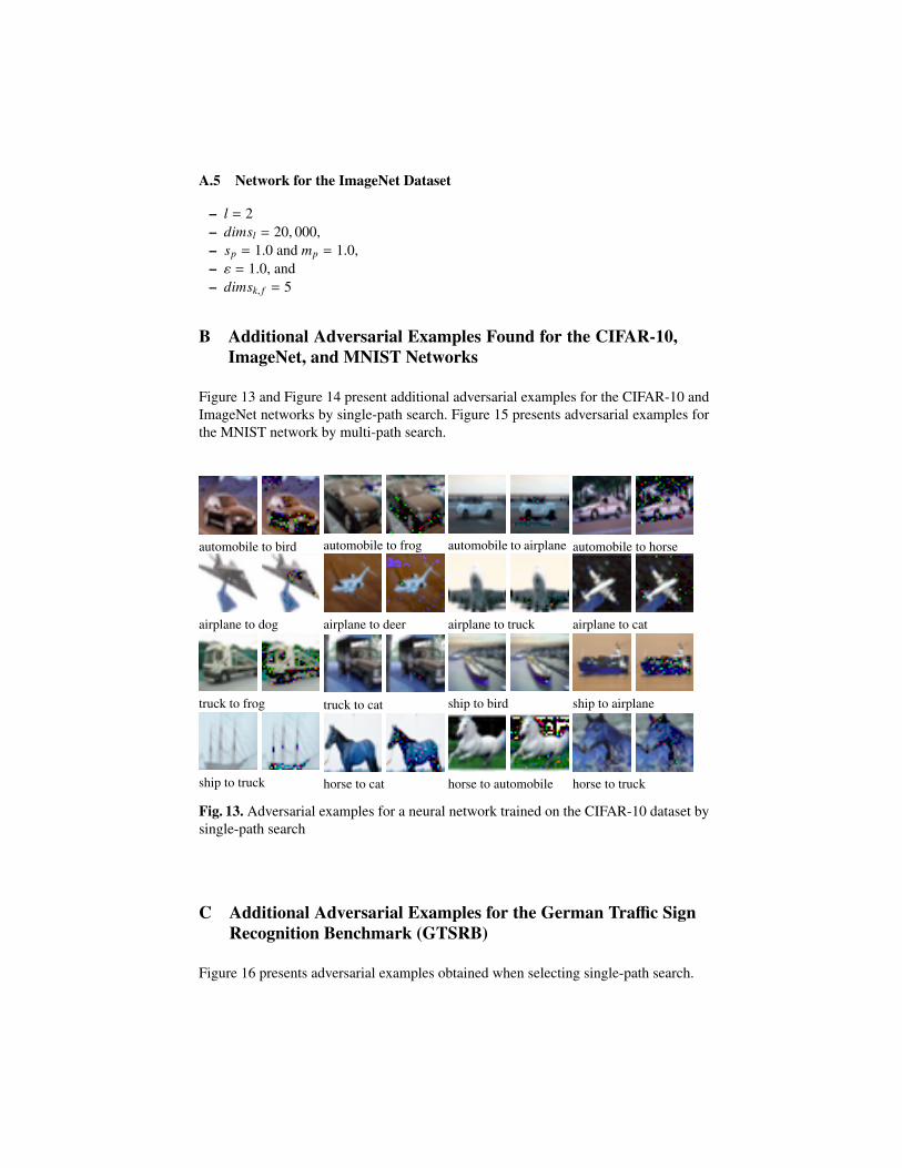
A.5 Network for the ImageNet Dataset

– l = 2– dimsl = 20, 000,– sp = 1.0 and mp = 1.0,– ε = 1.0, and– dimsk, f = 5

B Additional Adversarial Examples Found for the CIFAR-10,ImageNet, and MNIST Networks

Figure 13 and Figure 14 present additional adversarial examples for the CIFAR-10 andImageNet networks by single-path search. Figure 15 presents adversarial examples forthe MNIST network by multi-path search.

automobile to bird automobile to frog automobile to airplane automobile to horse

airplane to dog airplane to deer airplane to truck airplane to cat

truck to frog truck to cat ship to bird ship to airplane

ship to truck horse to cat horse to automobile horse to truck

Fig. 13. Adversarial examples for a neural network trained on the CIFAR-10 dataset bysingle-path search

C Additional Adversarial Examples for the German Traffic SignRecognition Benchmark (GTSRB)

Figure 16 presents adversarial examples obtained when selecting single-path search.

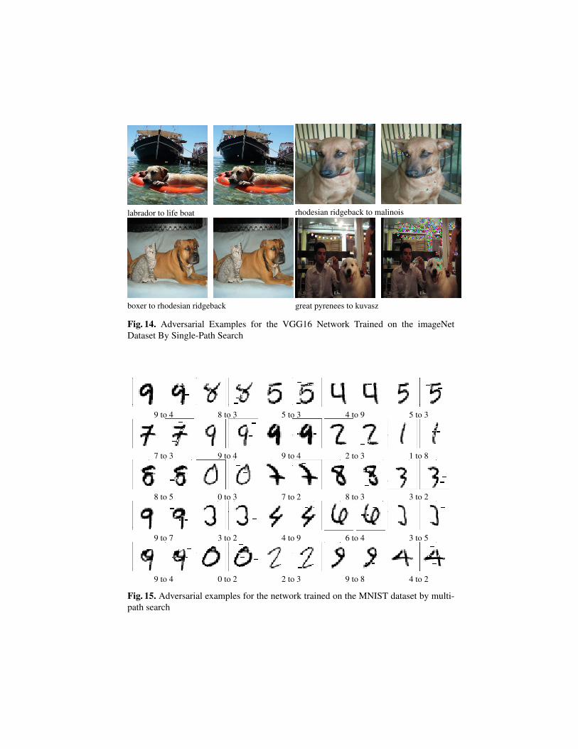
labrador to life boat rhodesian ridgeback to malinois

boxer to rhodesian ridgeback great pyrenees to kuvasz

Fig. 14. Adversarial Examples for the VGG16 Network Trained on the imageNetDataset By Single-Path Search

9 to 4 8 to 3 5 to 3 4 to 9 5 to 3

7 to 3 9 to 4 9 to 4 2 to 3 1 to 8

8 to 5 0 to 3 7 to 2 8 to 3 3 to 2

9 to 7 3 to 2 4 to 9 6 to 4 3 to 5

9 to 4 0 to 2 2 to 3 9 to 8 4 to 2

Fig. 15. Adversarial examples for the network trained on the MNIST dataset by multi-path search

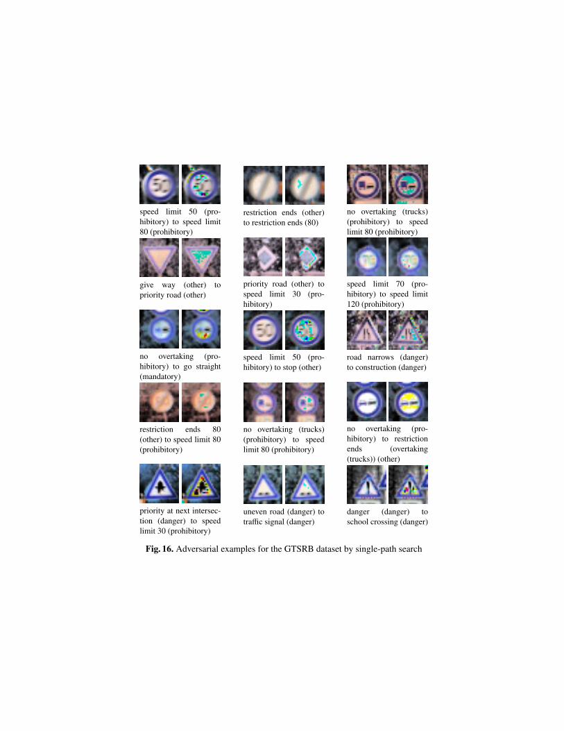
speed limit 50 (pro-hibitory) to speed limit80 (prohibitory)

restriction ends (other)to restriction ends (80)

no overtaking (trucks)(prohibitory) to speedlimit 80 (prohibitory)

give way (other) topriority road (other)

priority road (other) tospeed limit 30 (pro-hibitory)

speed limit 70 (pro-hibitory) to speed limit120 (prohibitory)

no overtaking (pro-hibitory) to go straight(mandatory)

speed limit 50 (pro-hibitory) to stop (other)

road narrows (danger)to construction (danger)

restriction ends 80(other) to speed limit 80(prohibitory)

no overtaking (trucks)(prohibitory) to speedlimit 80 (prohibitory)

no overtaking (pro-hibitory) to restrictionends (overtaking(trucks)) (other)

priority at next intersec-tion (danger) to speedlimit 30 (prohibitory)

uneven road (danger) totraffic signal (danger)

danger (danger) toschool crossing (danger)

Fig. 16. Adversarial examples for the GTSRB dataset by single-path search

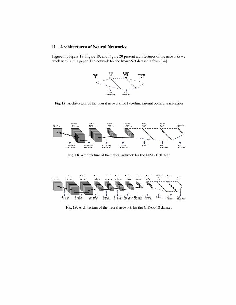
D Architectures of Neural Networks

Figure 17, Figure 18, Figure 19, and Figure 20 present architectures of the networks wework with in this paper. The network for the ImageNet dataset is from [34].

Fig. 17. Architecture of the neural network for two-dimensional point classification

Fig. 18. Architecture of the neural network for the MNIST dataset

Fig. 19. Architecture of the neural network for the CIFAR-10 dataset

Fig. 20. Architecture of the neural network for the GTSRB dataset