Multivariate analyses & decoding - · PDF fileMultivariate analyses & decoding Kay H....
51
Multivariate analyses & decoding Kay H. Brodersen Translational Neuromodeling Unit (TNU) Institute for Biomedical Engineering University of Zurich & ETH Zurich http://people.inf.ethz.ch/bkay
Transcript of Multivariate analyses & decoding - · PDF fileMultivariate analyses & decoding Kay H....

Multivariate analyses & decoding
Kay H. Brodersen
Translational Neuromodeling Unit (TNU) Institute for Biomedical Engineering University of Zurich & ETH Zurich
http://people.inf.ethz.ch/bkay
2
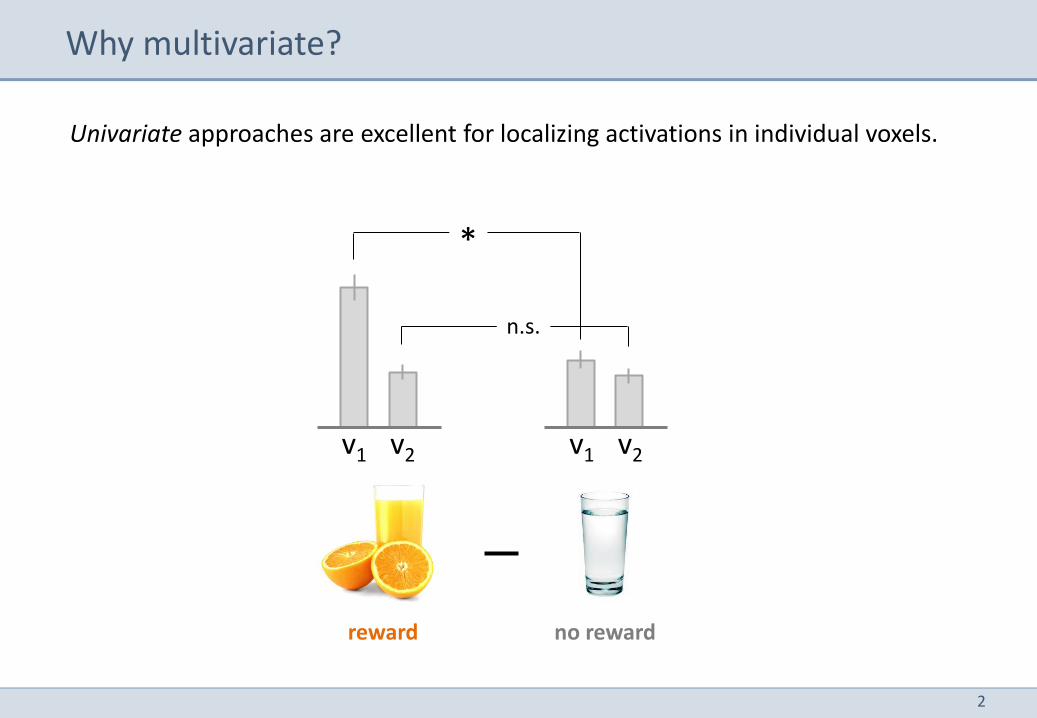
Univariate approaches are excellent for localizing activations in individual voxels.
Why multivariate?
v1 v2 v1 v2
reward no reward
*
n.s.
3
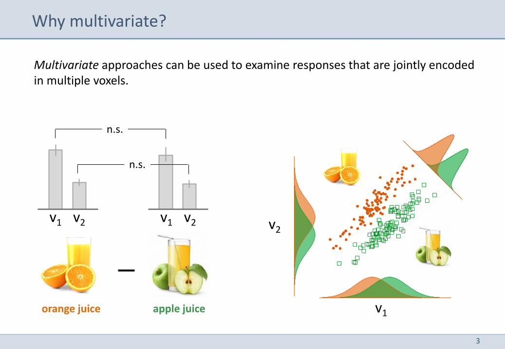
Multivariate approaches can be used to examine responses that are jointly encoded in multiple voxels.
Why multivariate?
v1 v2 v1 v2
n.s.
orange juice apple juice v1
v2
n.s.
4
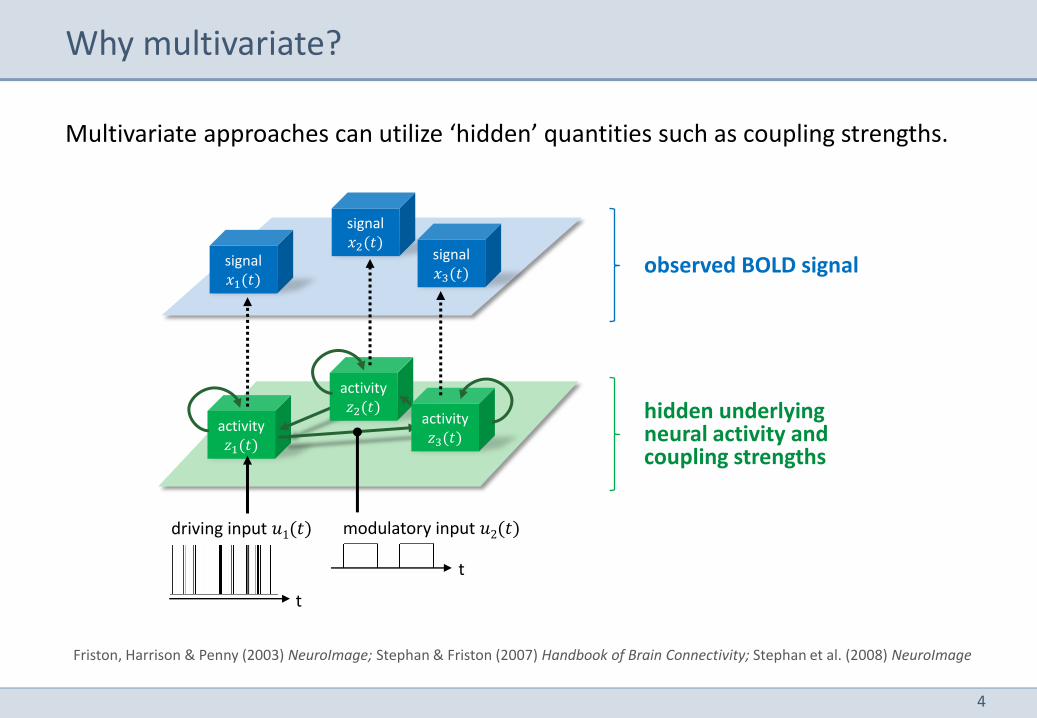
Multivariate approaches can utilize ‘hidden’ quantities such as coupling strengths.
Why multivariate?
activity 𝑧1(𝑡)
observed BOLD signal
hidden underlying neural activity and coupling strengths
t
driving input 𝑢1(𝑡) modulatory input 𝑢2(𝑡)
t
activity 𝑧2(𝑡)
activity 𝑧3(𝑡)
signal 𝑥1(𝑡)
signal 𝑥2(𝑡)
signal 𝑥3(𝑡)
Friston, Harrison & Penny (2003) NeuroImage; Stephan & Friston (2007) Handbook of Brain Connectivity; Stephan et al. (2008) NeuroImage
5
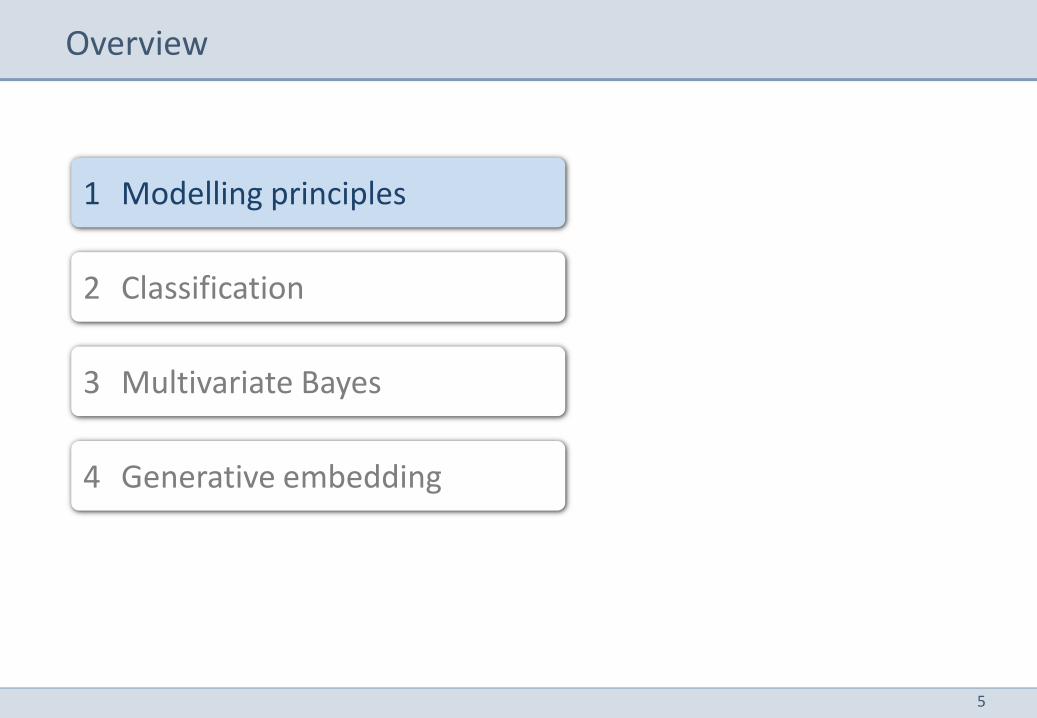
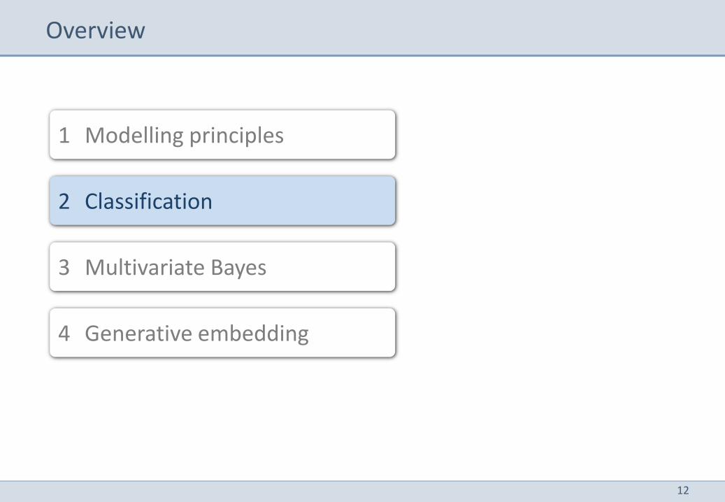
Overview
1 Modelling principles
2 Classification
3 Multivariate Bayes
4 Generative embedding
6
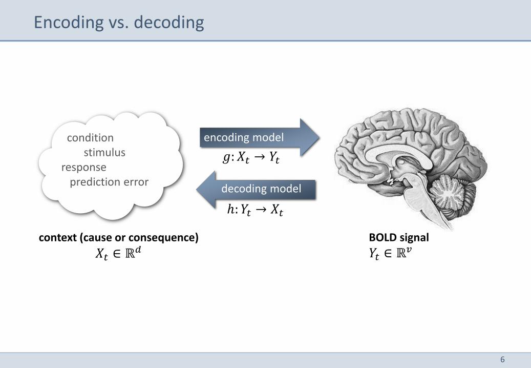
Encoding vs. decoding
context (cause or consequence)
𝑋𝑡 ∈ ℝ𝑑 BOLD signal
𝑌𝑡 ∈ ℝ𝑣
condition stimulus response prediction error
encoding model
decoding model
𝑔: 𝑋𝑡 → 𝑌𝑡
ℎ: 𝑌𝑡 → 𝑋𝑡
7
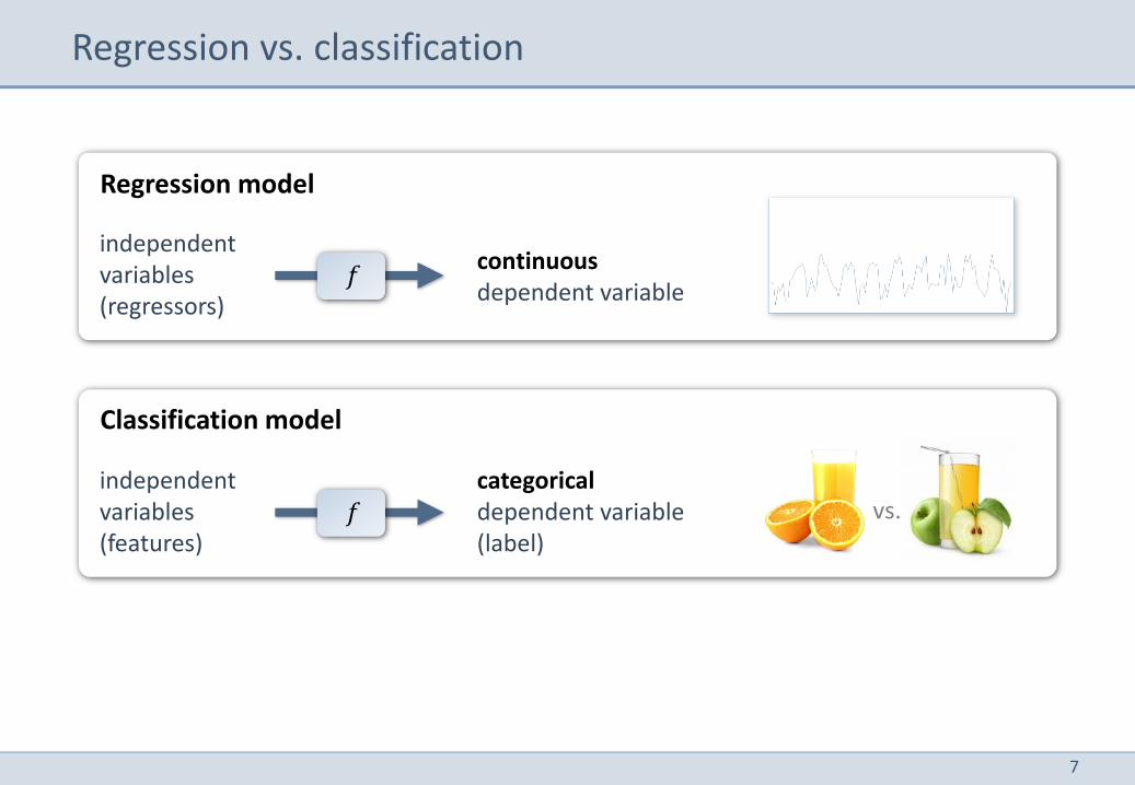
Regression vs. classification
Regression model
independent variables (regressors)
continuous dependent variable
Classification model
independent variables (features)
categorical dependent variable (label)
𝑓
𝑓 vs.
8
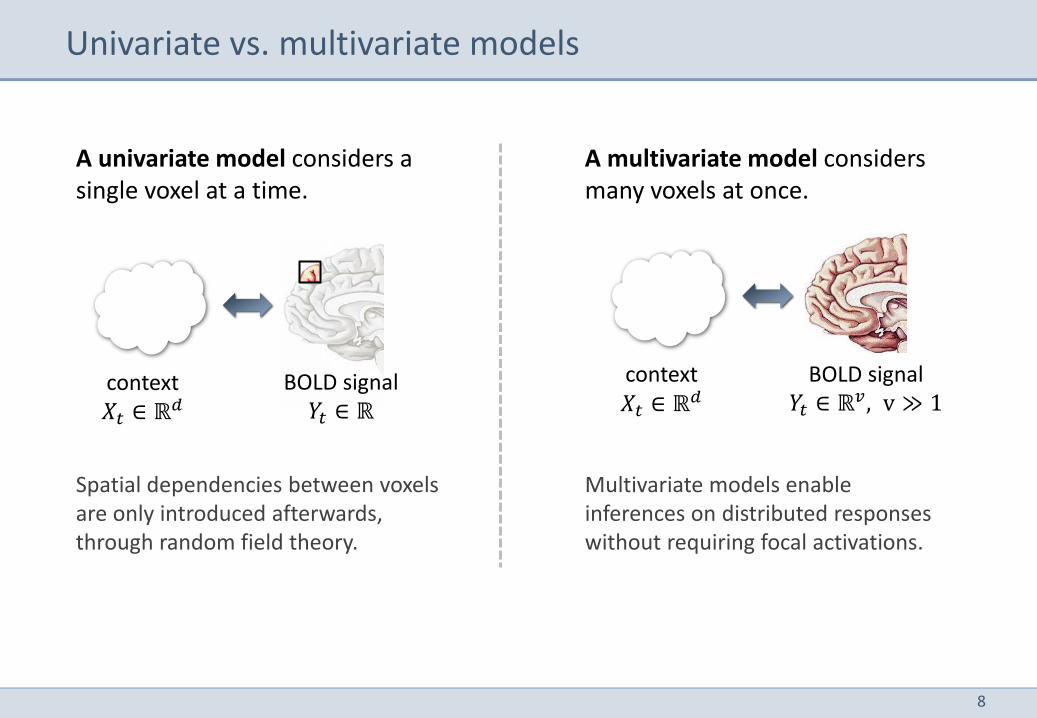
Univariate vs. multivariate models
BOLD signal 𝑌𝑡 ∈ ℝ𝑣, v ≫ 1
context 𝑋𝑡 ∈ ℝ𝑑
A univariate model considers a single voxel at a time.
A multivariate model considers many voxels at once.
Spatial dependencies between voxels are only introduced afterwards, through random field theory.
BOLD signal 𝑌𝑡 ∈ ℝ
context 𝑋𝑡 ∈ ℝ𝑑
Multivariate models enable inferences on distributed responses without requiring focal activations.
9
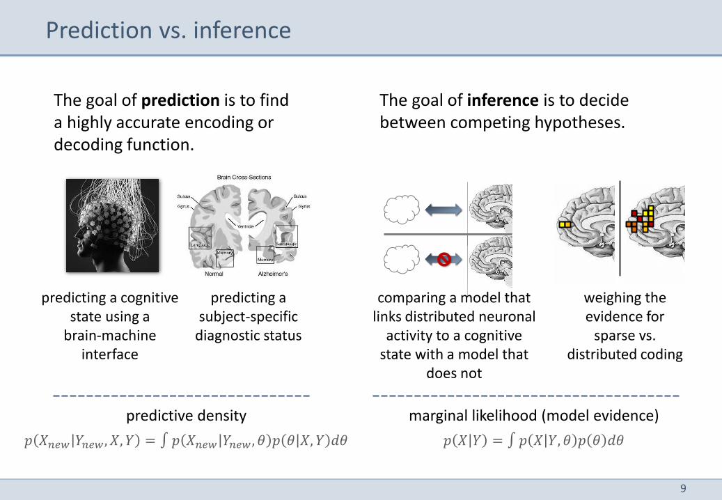
Prediction vs. inference
The goal of prediction is to find a highly accurate encoding or decoding function.
The goal of inference is to decide between competing hypotheses.
predicting a cognitive state using a
brain-machine interface
predicting a subject-specific
diagnostic status
predictive density
𝑝 𝑋𝑛𝑒𝑤 𝑌𝑛𝑒𝑤 , 𝑋, 𝑌 = ∫ 𝑝 𝑋𝑛𝑒𝑤 𝑌𝑛𝑒𝑤 , 𝜃 𝑝 𝜃 𝑋, 𝑌 𝑑𝜃
marginal likelihood (model evidence)
𝑝 𝑋 𝑌 = ∫ 𝑝 𝑋 𝑌, 𝜃 𝑝 𝜃 𝑑𝜃
comparing a model that links distributed neuronal
activity to a cognitive state with a model that
does not
weighing the evidence for
sparse vs. distributed coding
10
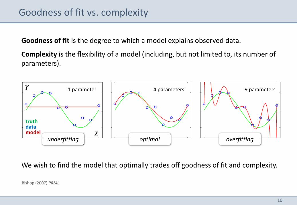
Goodness of fit vs. complexity
Goodness of fit is the degree to which a model explains observed data.
Complexity is the flexibility of a model (including, but not limited to, its number of parameters).
4 parameters 9 parameters
Bishop (2007) PRML
1 parameter
𝑋
𝑌
We wish to find the model that optimally trades off goodness of fit and complexity.
underfitting overfitting optimal
truth data model
11
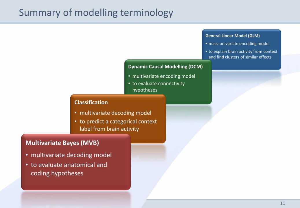
General Linear Model (GLM)
• mass-univariate encoding model
• to explain brain activity from context and find clusters of similar effects
Dynamic Causal Modelling (DCM)
• multivariate encoding model
• to evaluate connectivity hypotheses
Summary of modelling terminology
Classification
• multivariate decoding model
• to predict a categorical context label from brain activity
Multivariate Bayes (MVB)
• multivariate decoding model
• to evaluate anatomical and coding hypotheses
12
Overview
1 Modelling principles
2 Classification
3 Multivariate Bayes
4 Generative embedding
13
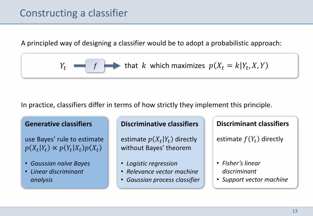
A principled way of designing a classifier would be to adopt a probabilistic approach:
Constructing a classifier
Generative classifiers
use Bayes’ rule to estimate 𝑝 𝑋𝑡 𝑌𝑡 ∝ 𝑝 𝑌𝑡 𝑋𝑡 𝑝 𝑋𝑡
• Gaussian naïve Bayes • Linear discriminant
analysis
Discriminative classifiers
estimate 𝑝 𝑋𝑡 𝑌𝑡 directly without Bayes’ theorem
• Logistic regression • Relevance vector machine • Gaussian process classifier
Discriminant classifiers
estimate 𝑓 𝑌𝑡 directly
• Fisher’s linear discriminant
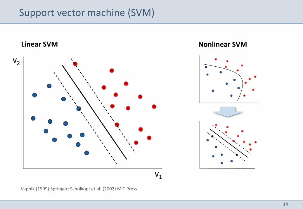
• Support vector machine
𝑓 𝑌𝑡 that 𝑘 which maximizes 𝑝 𝑋𝑡 = 𝑘 𝑌𝑡, 𝑋, 𝑌
In practice, classifiers differ in terms of how strictly they implement this principle.
14
Support vector machine (SVM)
Vapnik (1999) Springer; Schölkopf et al. (2002) MIT Press
Nonlinear SVM Linear SVM
v1
v2
15
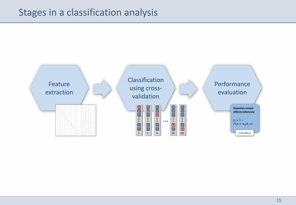
Stages in a classification analysis
Feature extraction
Classification using cross-validation
Performance evaluation
Bayesian mixed-effects inference
𝑝 = 1 − 𝑃 𝜋 > 𝜋0 𝑘, 𝑛
mixed effects
16
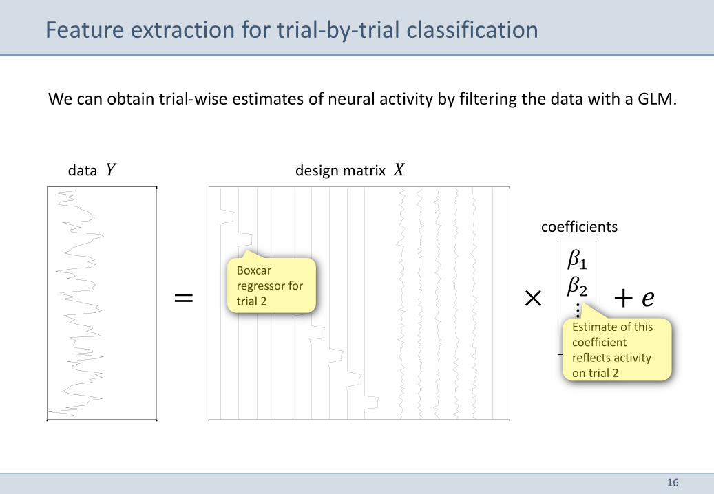
We can obtain trial-wise estimates of neural activity by filtering the data with a GLM.
Feature extraction for trial-by-trial classification
=
data 𝑌 design matrix 𝑋
𝛽1𝛽2⋮𝛽𝑝
× + 𝑒
coefficients
Boxcar regressor for trial 2
Estimate of this coefficient reflects activity on trial 2
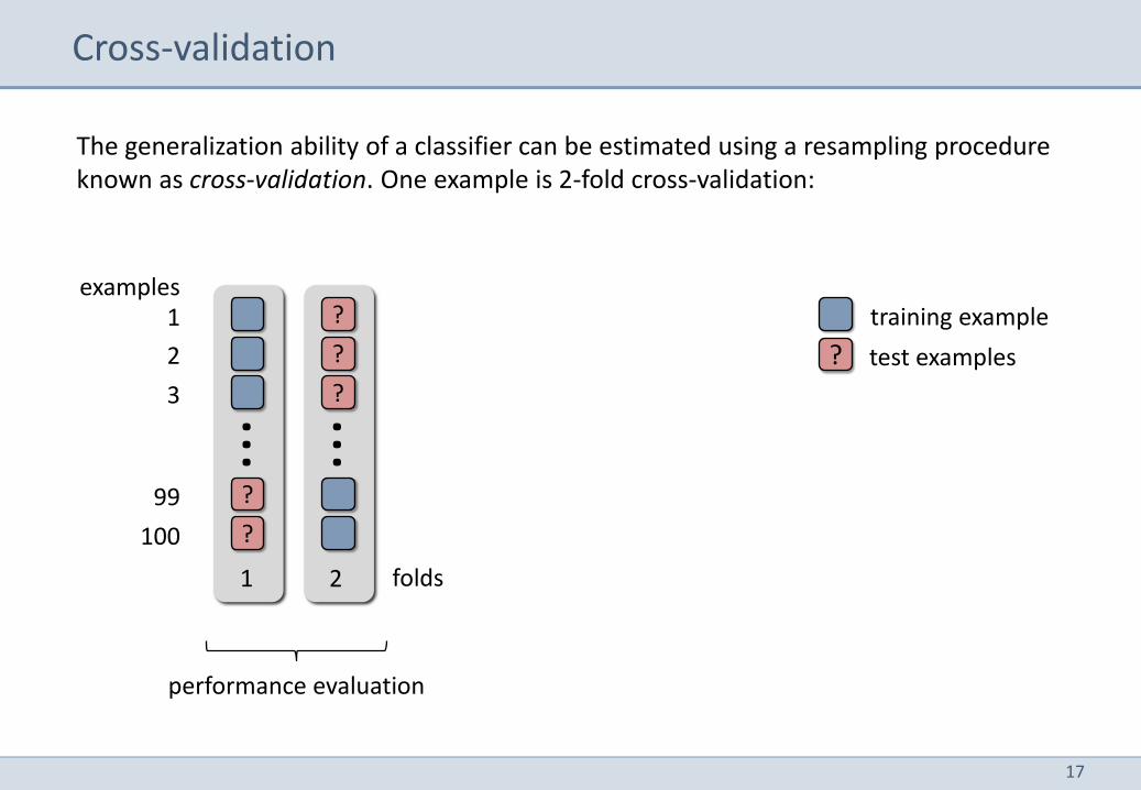
17
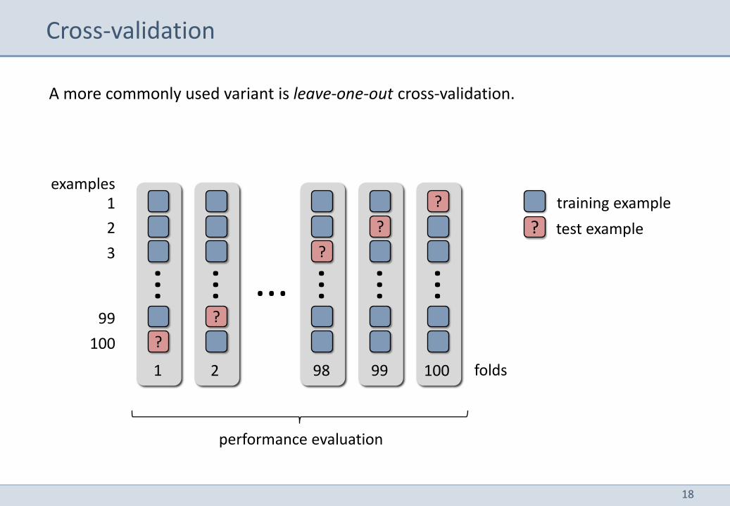
The generalization ability of a classifier can be estimated using a resampling procedure known as cross-validation. One example is 2-fold cross-validation:
Cross-validation
examples 1
2
3
99
100
?
training example
test examples
folds
?
?
1
...
?
?
?
2
...
performance evaluation
18
A more commonly used variant is leave-one-out cross-validation.
Cross-validation
examples 1
2
3
99
100
?
training example
test example
? ... 98
?
... 99
?
...
100
...
folds
?
1
...
?
2
...
performance evaluation
19
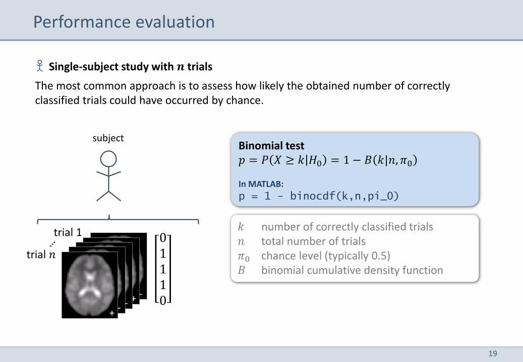
Single-subject study with 𝒏 trials
The most common approach is to assess how likely the obtained number of correctly classified trials could have occurred by chance.
Performance evaluation
𝑘 number of correctly classified trials 𝑛 total number of trials 𝜋0 chance level (typically 0.5) 𝐵 binomial cumulative density function
Binomial test 𝑝 = 𝑃 𝑋 ≥ 𝑘 𝐻0 = 1 − 𝐵 𝑘|𝑛, 𝜋0 In MATLAB:
p = 1 - binocdf(k,n,pi_0)
subject
- + - - +
trial 𝑛
trial 1 01110
20
Performance evaluation
subject 1
- + - - +
trial 𝑛
trial 1
population
01110
subject 2
11011
subject 3
01100
subject 4
11111
subject 𝑚
…
…
01110
21
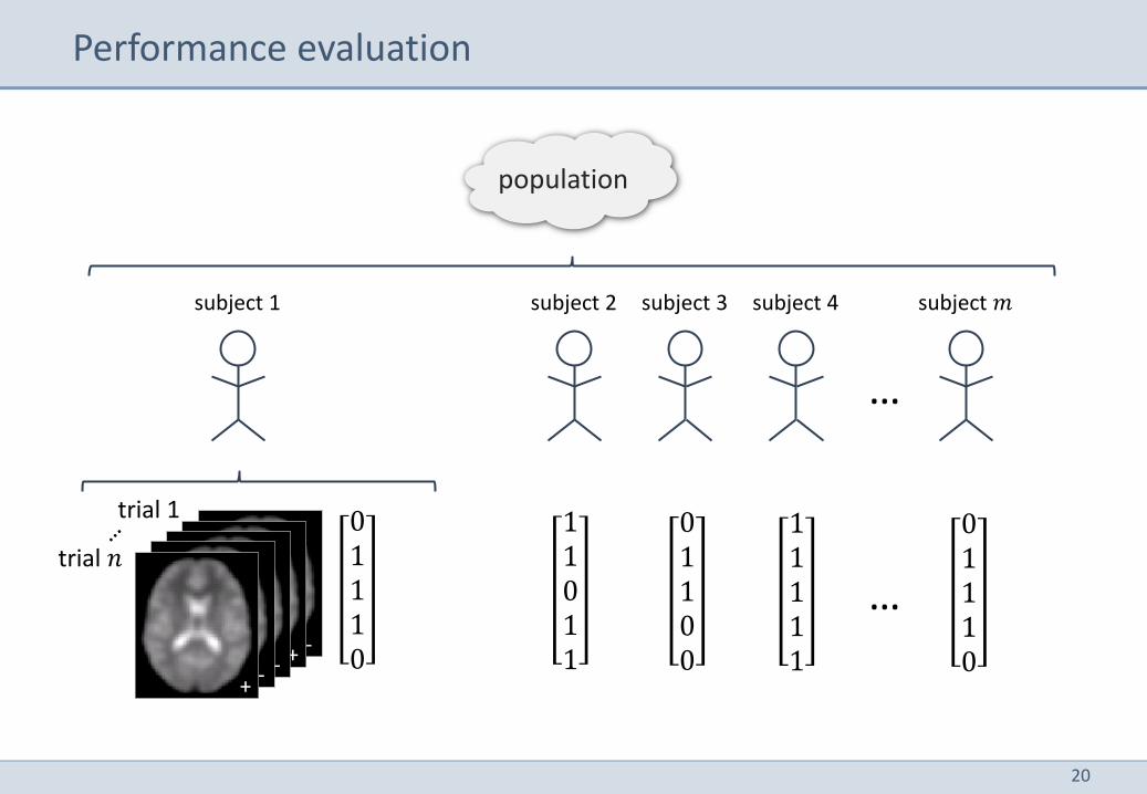
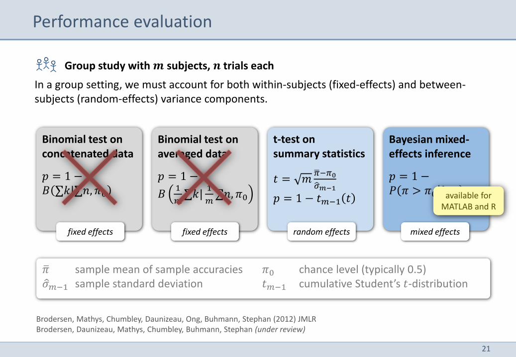
Group study with 𝒎 subjects, 𝒏 trials each
In a group setting, we must account for both within-subjects (fixed-effects) and between-subjects (random-effects) variance components.
Performance evaluation
𝜋 sample mean of sample accuracies 𝜋0 chance level (typically 0.5) 𝜎 𝑚−1 sample standard deviation 𝑡𝑚−1 cumulative Student’s 𝑡-distribution
t-test on summary statistics
𝑡 = 𝑚𝜋 −𝜋0
𝜎 𝑚−1
𝑝 = 1 − 𝑡𝑚−1 𝑡
Binomial test on concatenated data
𝑝 = 1 − 𝐵 ∑𝑘|∑𝑛, 𝜋0
Binomial test on averaged data
𝑝 = 1 −
𝐵1
𝑚∑𝑘|
1
𝑚∑𝑛, 𝜋0
Bayesian mixed-effects inference
𝑝 = 1 − 𝑃 𝜋 > 𝜋0 𝑘, 𝑛
fixed effects random effects fixed effects mixed effects
Brodersen, Mathys, Chumbley, Daunizeau, Ong, Buhmann, Stephan (2012) JMLR Brodersen, Daunizeau, Mathys, Chumbley, Buhmann, Stephan (under review)
available for MATLAB and R
22
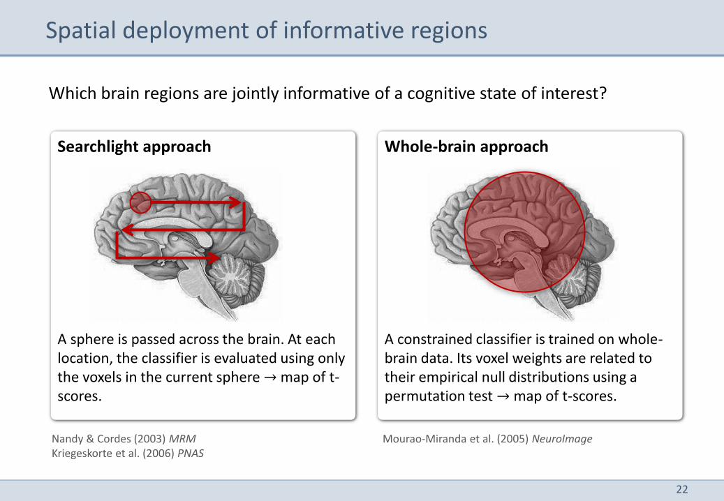
Searchlight approach
A sphere is passed across the brain. At each location, the classifier is evaluated using only the voxels in the current sphere → map of t-scores.
Whole-brain approach
A constrained classifier is trained on whole-brain data. Its voxel weights are related to their empirical null distributions using a permutation test → map of t-scores.
Which brain regions are jointly informative of a cognitive state of interest?
Spatial deployment of informative regions
Nandy & Cordes (2003) MRM Kriegeskorte et al. (2006) PNAS
Mourao-Miranda et al. (2005) NeuroImage
23
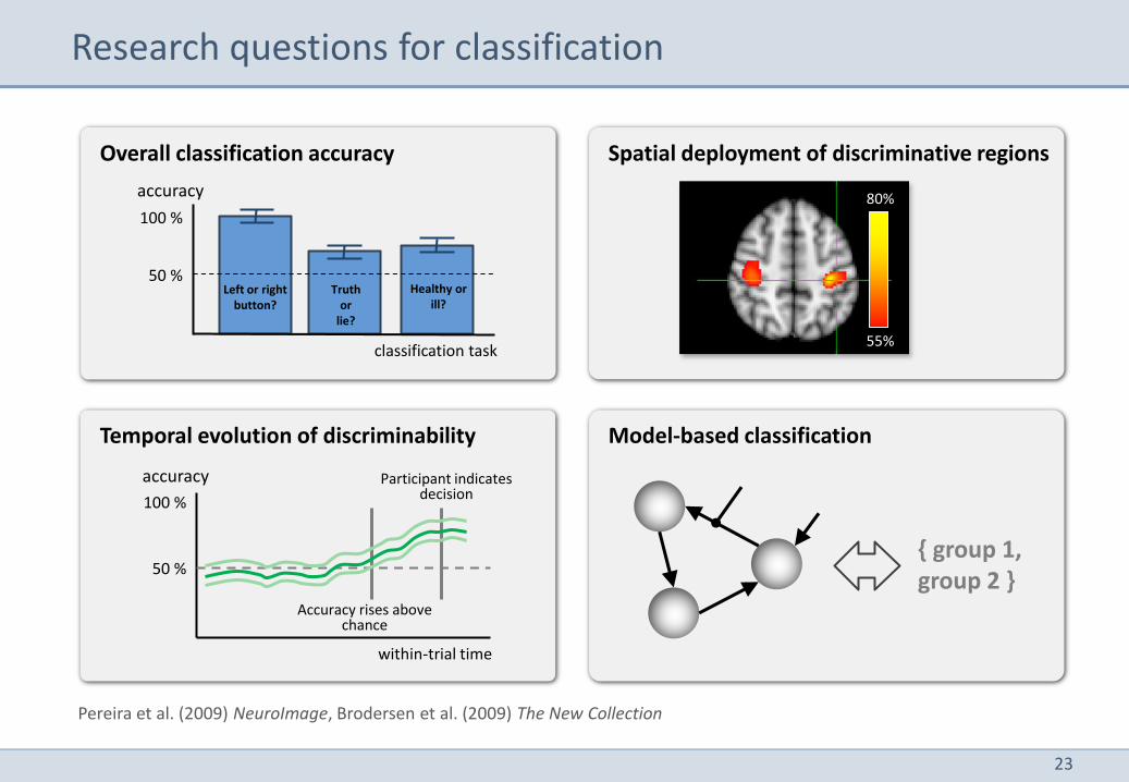
Research questions for classification
Temporal evolution of discriminability Model-based classification
accuracy
50 %
100 %
within-trial time
Accuracy rises above chance
Participant indicates decision
Overall classification accuracy Spatial deployment of discriminative regions
80%
55%
accuracy
50 %
100 %
classification task
Truth or
lie?
Left or right button?
Healthy or ill?
Pereira et al. (2009) NeuroImage, Brodersen et al. (2009) The New Collection
{ group 1, group 2 }
24
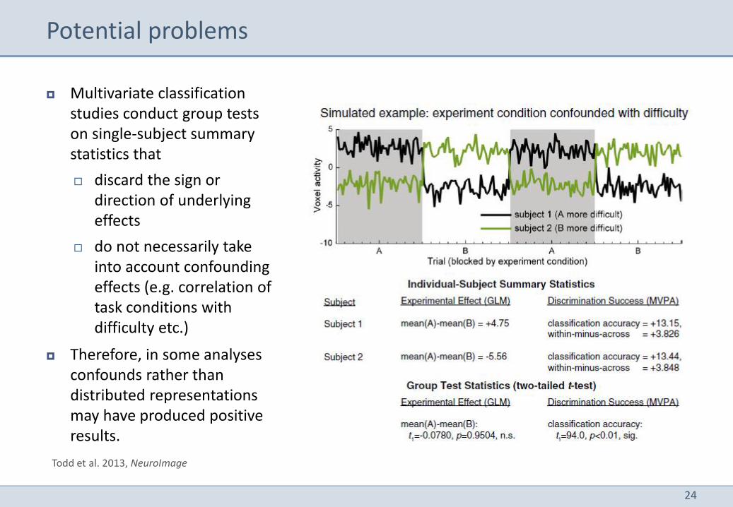
Multivariate classification studies conduct group tests on single-subject summary statistics that
discard the sign or direction of underlying effects
do not necessarily take into account confounding effects (e.g. correlation of task conditions with difficulty etc.)
Therefore, in some analyses confounds rather than distributed representations may have produced positive results.
Potential problems
Todd et al. 2013, NeuroImage
25
Overview
1 Modelling principles
2 Classification
3 Multivariate Bayes
4 Generative embedding
26
Multivariate Bayes
Mike West
SPM brings multivariate analyses into the conventional inference framework of Bayesian hierarchical models and their inversion.
27
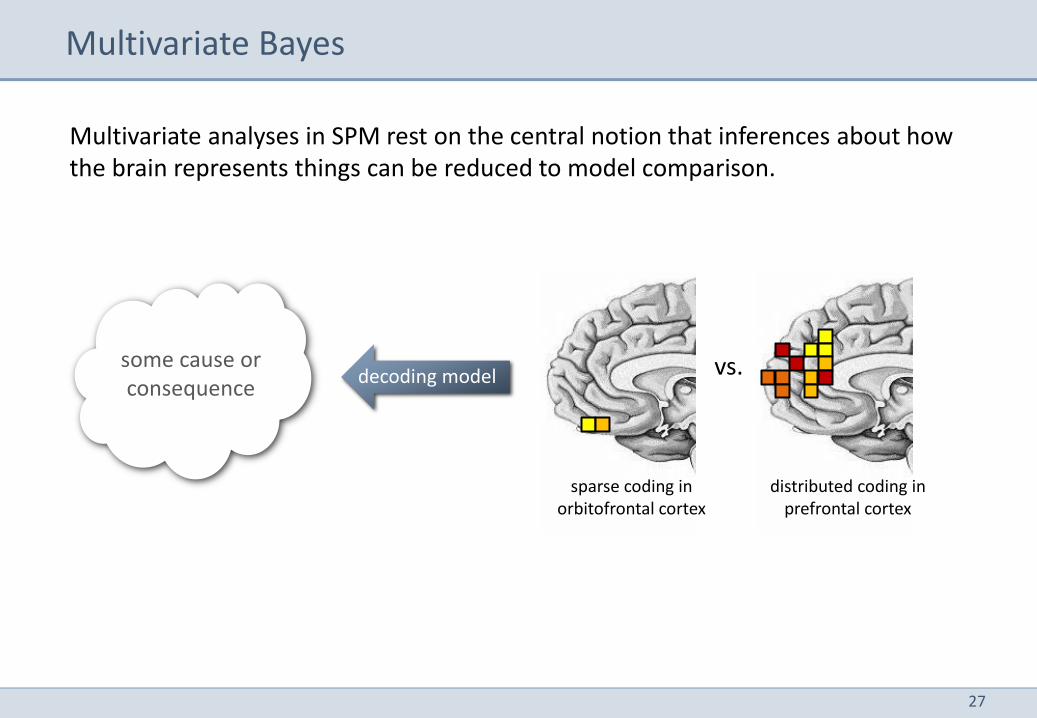
Multivariate Bayes
some cause or consequence
decoding model
Multivariate analyses in SPM rest on the central notion that inferences about how the brain represents things can be reduced to model comparison.
vs.
sparse coding in orbitofrontal cortex
distributed coding in prefrontal cortex
28
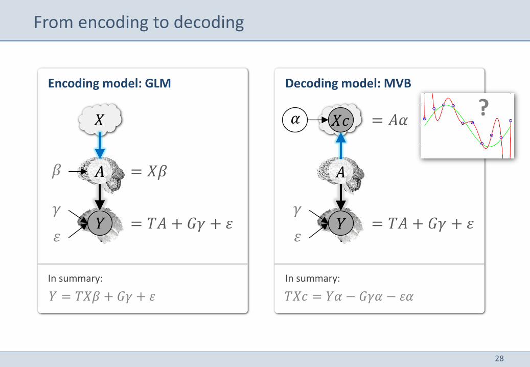
From encoding to decoding
Encoding model: GLM Decoding model: MVB
𝑌
= 𝑋𝛽
= 𝑇𝐴 + 𝐺𝛾 + 𝜀 𝛾
𝜀
𝛽
𝛼 𝑋
𝐴
𝑌
= 𝐴𝛼
= 𝑇𝐴 + 𝐺𝛾 + 𝜀
𝑋𝑐
𝐴
𝑌 = 𝑇𝑋𝛽 + 𝐺𝛾 + 𝜀 𝑇𝑋𝑐 = 𝑌𝛼 − 𝐺𝛾𝛼 − 𝜀𝛼
𝛾
𝜀
In summary: In summary:
?
29
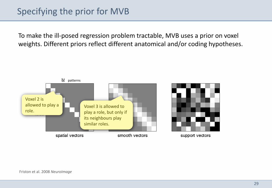
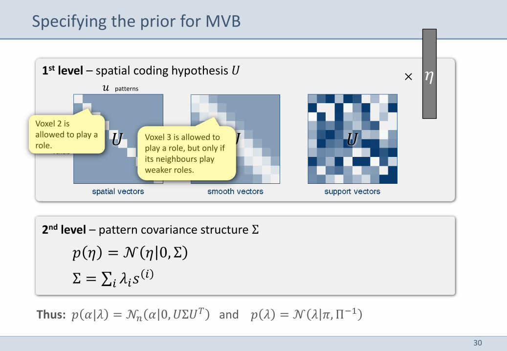
Specifying the prior for MVB
To make the ill-posed regression problem tractable, MVB uses a prior on voxel weights. Different priors reflect different anatomical and/or coding hypotheses.
𝑛 voxels
𝑢 patterns
Voxel 3 is allowed to play a role, but only if its neighbours play similar roles.
Voxel 2 is allowed to play a role.
Friston et al. 2008 NeuroImage
30
Specifying the prior for MVB
1st level – spatial coding hypothesis 𝑈
2nd level – pattern covariance structure Σ
𝑝 𝜂 = 𝒩 𝜂 0, Σ
Σ = ∑ 𝜆𝑖𝑠𝑖
𝑖
𝜂 ×
𝑛 voxels
𝑢 patterns
Thus: 𝑝 𝛼|𝜆 = 𝒩𝑛 𝛼 0, 𝑈Σ𝑈𝑇 and 𝑝 𝜆 = 𝒩 𝜆 𝜋, Π−1
𝑈 𝑈 𝑈 Voxel 3 is allowed to play a role, but only if its neighbours play weaker roles.
Voxel 2 is allowed to play a role.
31
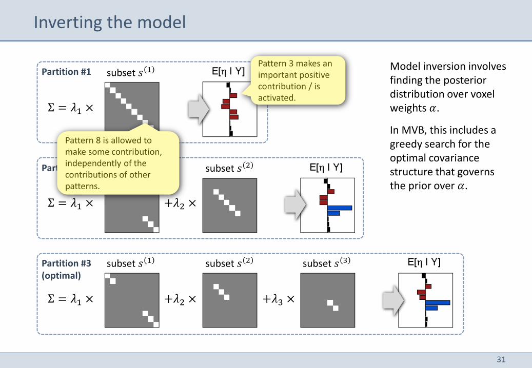
Inverting the model
Partition #1
Partition #2
Partition #3 (optimal)
Σ = 𝜆1 ×
Σ = 𝜆1 ×
Σ = 𝜆1 ×
+𝜆2 ×
+𝜆2 × +𝜆3 ×
Model inversion involves finding the posterior distribution over voxel weights 𝛼.
In MVB, this includes a greedy search for the optimal covariance structure that governs the prior over 𝛼.
subset 𝑠 1 subset 𝑠 2
subset 𝑠 1 subset 𝑠 2 subset 𝑠 3
subset 𝑠 1
Pattern 8 is allowed to make some contribution, independently of the contributions of other patterns.
Pattern 3 makes an important positive contribution / is activated.
32
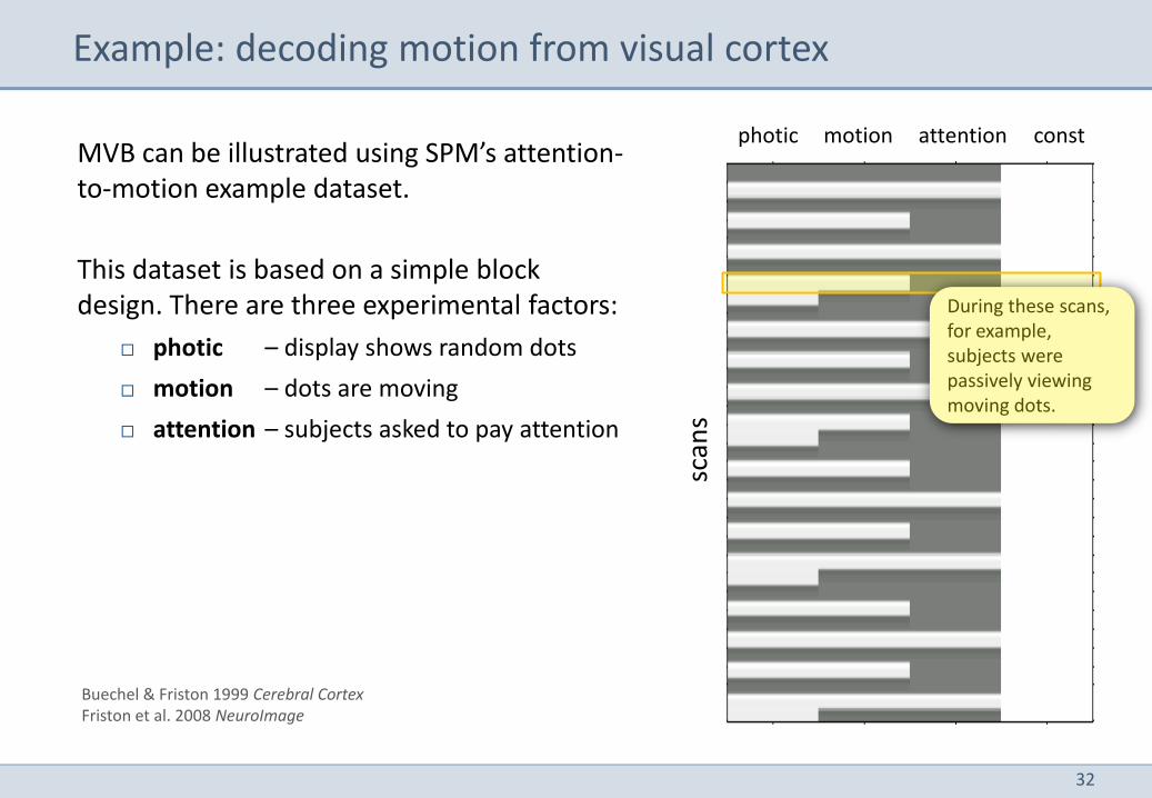
MVB can be illustrated using SPM’s attention-to-motion example dataset.
This dataset is based on a simple block design. There are three experimental factors:
photic – display shows random dots
motion – dots are moving
attention – subjects asked to pay attention
Example: decoding motion from visual cortex
scan
s
photic motion attention const
Buechel & Friston 1999 Cerebral Cortex Friston et al. 2008 NeuroImage
During these scans, for example, subjects were passively viewing moving dots.
33
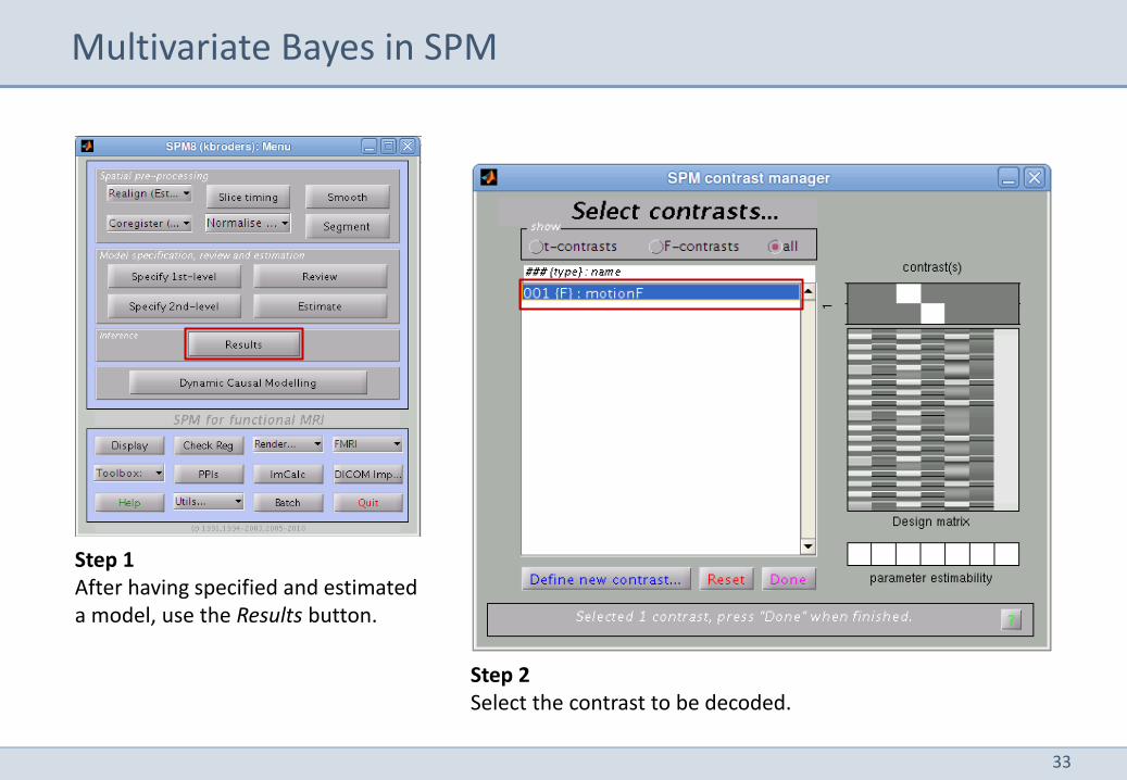
Multivariate Bayes in SPM
Step 1 After having specified and estimated a model, use the Results button.
Step 2 Select the contrast to be decoded.
34
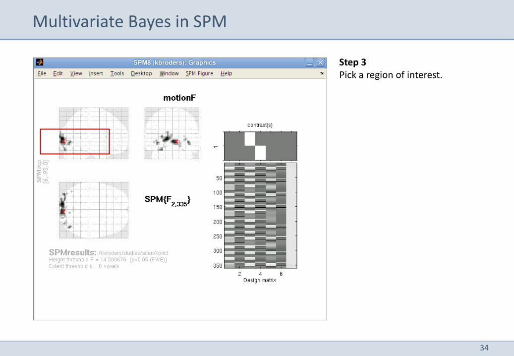
Multivariate Bayes in SPM
Step 3 Pick a region of interest.
35
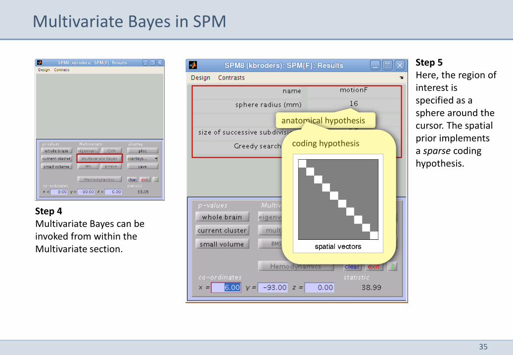
Multivariate Bayes in SPM
Step 4 Multivariate Bayes can be invoked from within the Multivariate section.
Step 5 Here, the region of interest is specified as a sphere around the cursor. The spatial prior implements a sparse coding hypothesis.
anatomical hypothesis
coding hypothesis
36
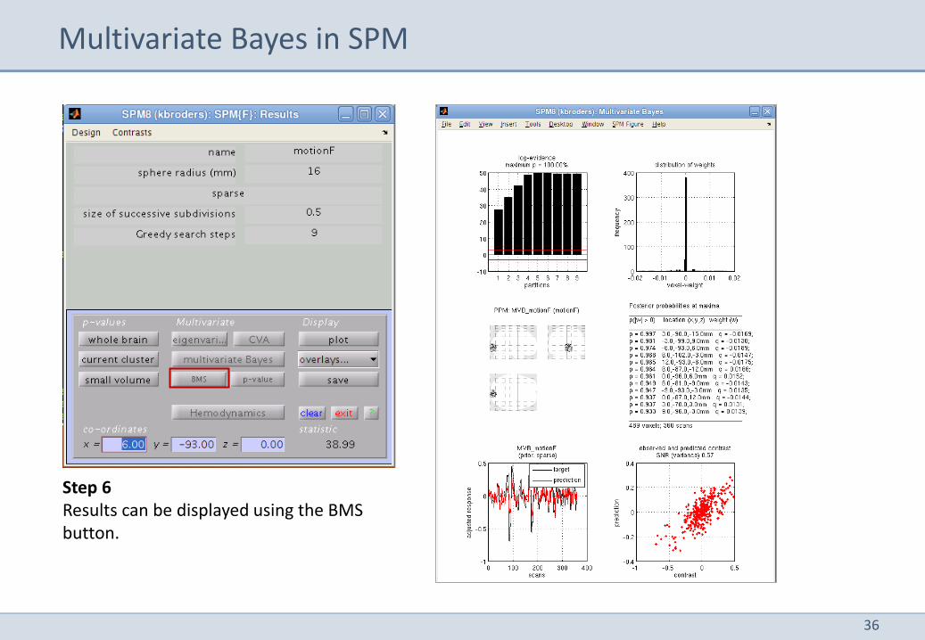
Multivariate Bayes in SPM
Step 6 Results can be displayed using the BMS button.
37
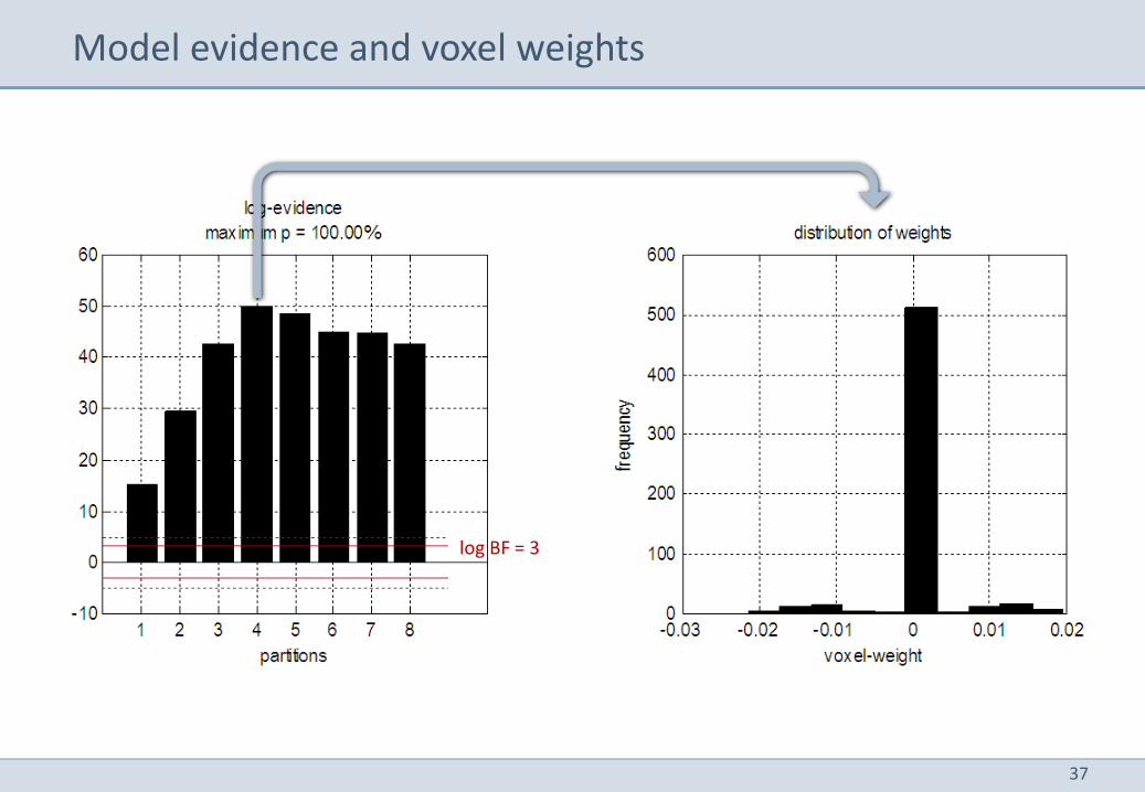
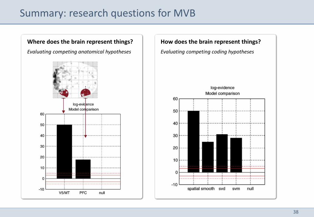
Model evidence and voxel weights
log BF = 3
38
Summary: research questions for MVB
How does the brain represent things?
Evaluating competing coding hypotheses
Where does the brain represent things?
Evaluating competing anatomical hypotheses
39
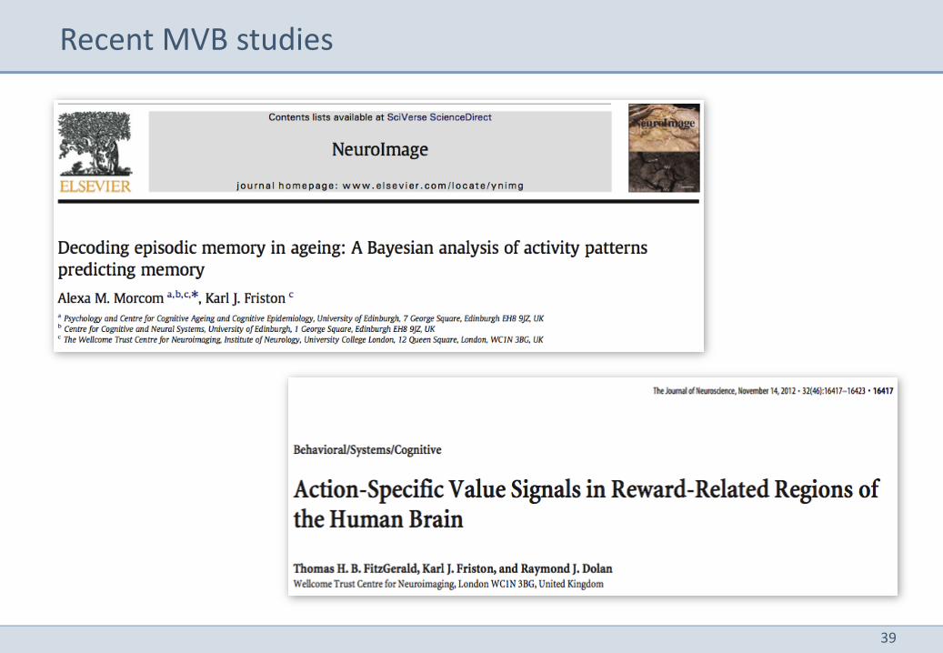
Recent MVB studies
40
Overview
1 Modelling principles
2 Classification
3 Multivariate Bayes
4 Generative embedding
41
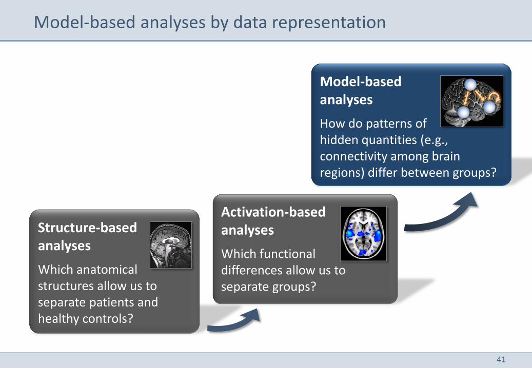
Model-based analyses by data representation
Model-based analyses
How do patterns of hidden quantities (e.g., connectivity among brain regions) differ between groups?
Structure-based analyses
Which anatomical structures allow us to separate patients and healthy controls?
Activation-based analyses
Which functional differences allow us to separate groups?
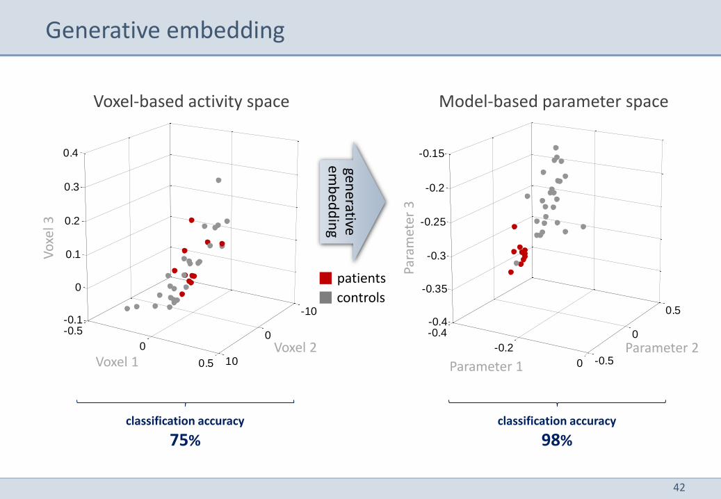
42
Generative embedding
-10
0
10
-0.5
0
0.5
-0.1
0
0.1
0.2
0.3
0.4
-0.4
-0.2
0 -0.5
0
0.5-0.4
-0.35
-0.3
-0.25
-0.2
-0.15
-10
0
10
-0.5
0
0.5
-0.1
0
0.1
0.2
0.3
0.4
-0.4
-0.2
0 -0.5
0
0.5-0.4
-0.35
-0.3
-0.25
-0.2
-0.15
generative
emb
ed
din
g
Para
met
er 3
Vo
xel 3
Parameter 1 Voxel 1 Voxel 2 Parameter 2
controls
patients
Voxel-based activity space Model-based parameter space
classification accuracy
98% classification accuracy
75%
43
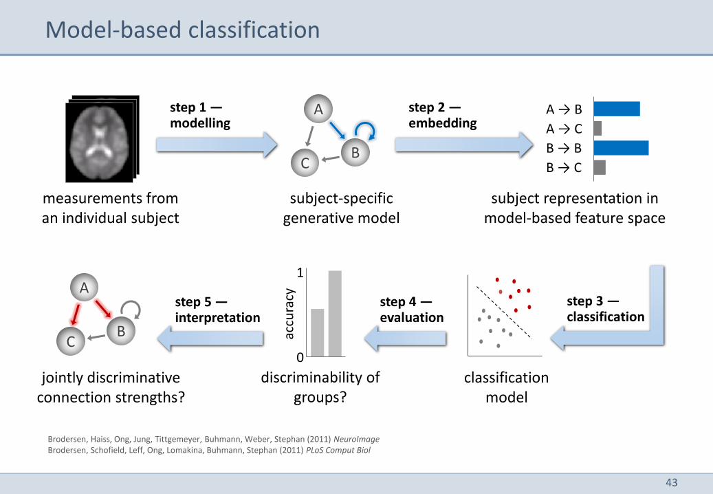
Model-based classification
Brodersen, Haiss, Ong, Jung, Tittgemeyer, Buhmann, Weber, Stephan (2011) NeuroImage Brodersen, Schofield, Leff, Ong, Lomakina, Buhmann, Stephan (2011) PLoS Comput Biol
step 2 — embedding
step 1 — modelling
measurements from an individual subject
subject-specific generative model
subject representation in model-based feature space
A → B
A → C
B → B
B → C
A
C B
step 3 — classification
A
C B
jointly discriminative connection strengths?
step 5 — interpretation
classification model
1
0
discriminability of groups?
accu
racy
step 4 — evaluation
44
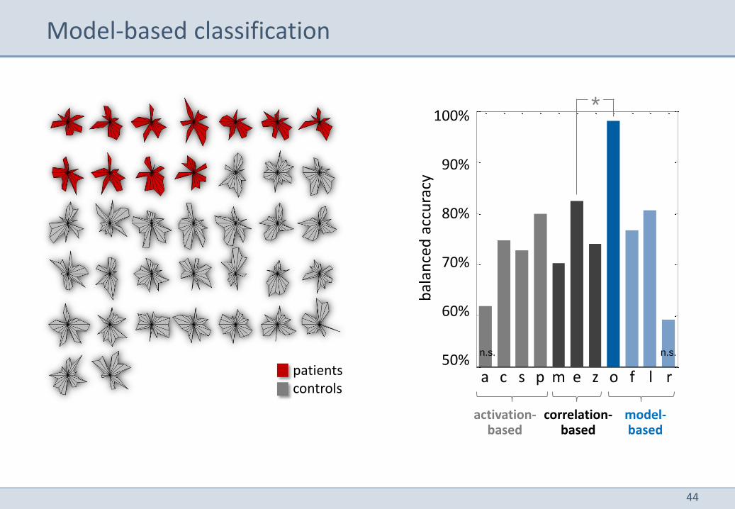
Model-based classification
patients controls
16218917734729133230781 24338936050
60
70
80
90
100
bala
nced
accu
racy
activation- based
correlation- based
model- based
a c s p m e z o f l r
bal
ance
d a
ccu
racy
100%
50%
90%
80%
70%
60%
n.s. n.s.
*
45
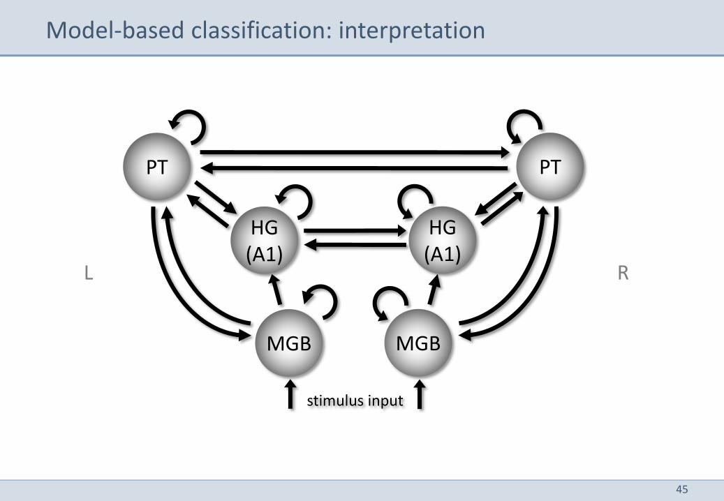
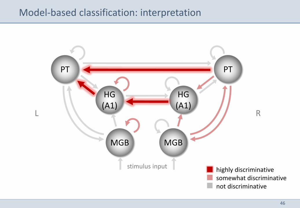
Model-based classification: interpretation
MGB
PT
HG (A1)
MGB
PT
HG (A1)
stimulus input
L R
46
Model-based classification: interpretation
MGB
PT
HG (A1)
MGB
PT
HG (A1)
stimulus input
L R
highly discriminative somewhat discriminative not discriminative
47
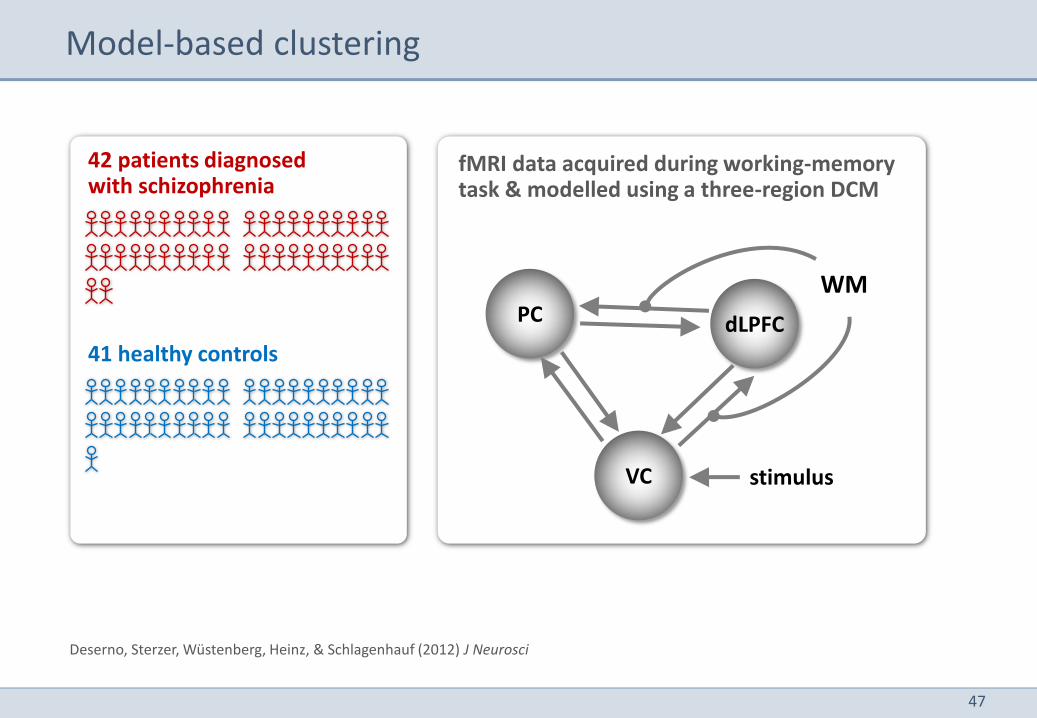
Model-based clustering
Deserno, Sterzer, Wüstenberg, Heinz, & Schlagenhauf (2012) J Neurosci
PC dLPFC
VC
WM
stimulus
fMRI data acquired during working-memory task & modelled using a three-region DCM
42 patients diagnosed with schizophrenia
41 healthy controls
48
0
0.2
0.4
0.6
0.8
1
bala
nced a
ccura
cy
1 2 3 4 5 6 7 80
20
40
60
80
100
120
log m
odel evid
ence
1 2 3 4 5 6 7 80
0.2
0.4
0.6
0.8
1
bala
nced p
urity
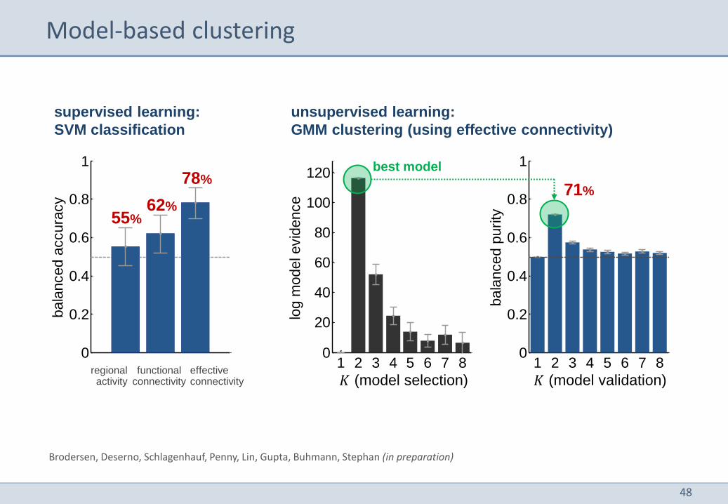
Model-based clustering
0
0.2
0.4
0.6
0.8
1
bala
nced a
ccura
cy
1 2 3 4 5 6 7 80
20
40
60
80
100
120
log m
odel evid
ence
1 2 3 4 5 6 7 80
0.2
0.4
0.6
0.8
1
bala
nced p
urity
0
0.2
0.4
0.6
0.8
1
bala
nced a
ccura
cy
1 2 3 4 5 6 7 80
20
40
60
80
100
120
log m
odel evid
ence
1 2 3 4 5 6 7 80
0.2
0.4
0.6
0.8
1
bala
nced p
urity
functional connectivity
effective connectivity
78%
71%
𝐾 (model selection) 𝐾 (model validation)
best model
71%
supervised learning:
SVM classification
unsupervised learning:
GMM clustering (using effective connectivity)
62%
78%
55%
regional activity
Brodersen, Deserno, Schlagenhauf, Penny, Lin, Gupta, Buhmann, Stephan (in preparation)
49
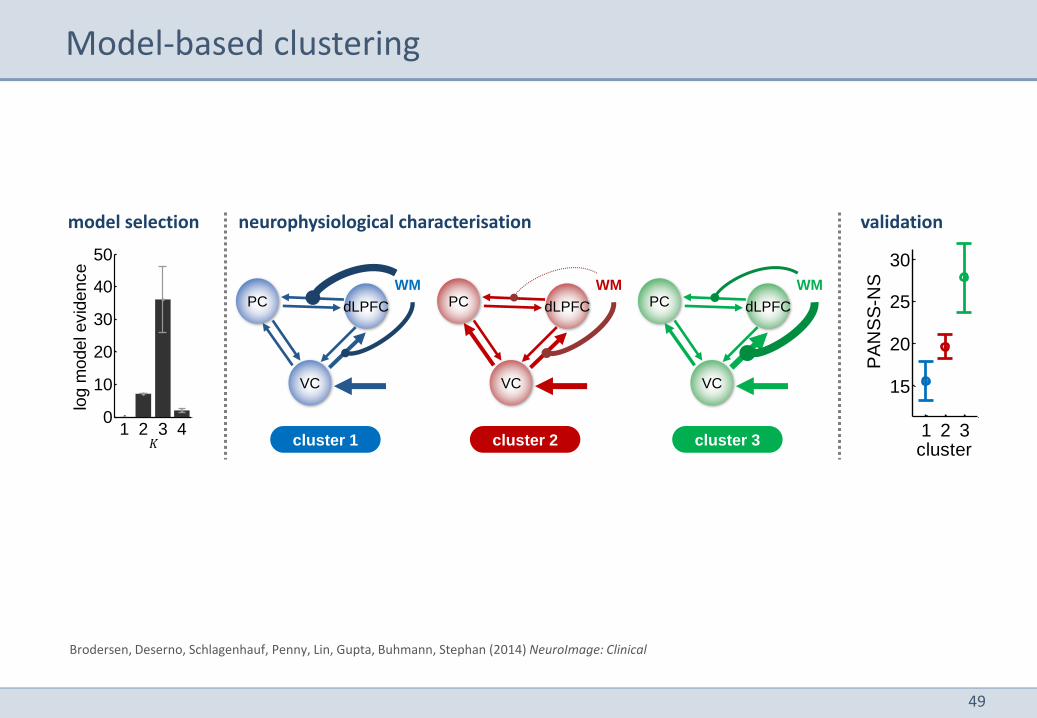
Model-based clustering
Brodersen, Deserno, Schlagenhauf, Penny, Lin, Gupta, Buhmann, Stephan (2014) NeuroImage: Clinical
1 2 3 40
10
20
30
40
50
log m
odel evid
ence
1 2 3 40
0.5
1
bala
nced p
urity
𝐾
model selection
PC dLPFC
VC
WM
cluster 1
PC dLPFC
VC
WM
cluster 2
PC dLPFC
VC
WM
cluster 3
neurophysiological characterisation validation
1 2 3
15
20
25
30
PA
NS
S-N
S
cluster
50
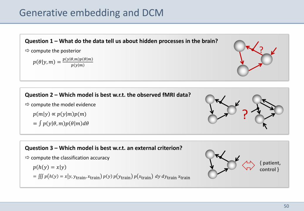
Question 1 – What do the data tell us about hidden processes in the brain?
compute the posterior
𝑝 𝜃 𝑦,𝑚 =𝑝 𝑦 𝜃,𝑚 𝑝 𝜃 𝑚
𝑝 𝑦 𝑚
Generative embedding and DCM
?
?
Question 2 – Which model is best w.r.t. the observed fMRI data?
compute the model evidence
𝑝 𝑚 𝑦 ∝ 𝑝 𝑦 𝑚 𝑝(𝑚)
= ∫ 𝑝 𝑦 𝜃,𝑚 𝑝 𝜃 𝑚 𝑑𝜃
Question 3 – Which model is best w.r.t. an external criterion?
compute the classification accuracy
𝑝 ℎ 𝑦 = 𝑥 𝑦
= 𝑝 ℎ 𝑦 = 𝑥 𝑦, 𝑦train, 𝑥train 𝑝 𝑦 𝑝 𝑦train 𝑝 𝑥train 𝑑𝑦 𝑑𝑦train 𝑥train
{ patient, control }
51
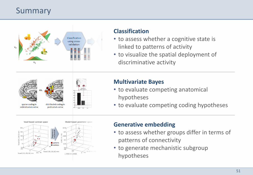
Summary
Classification • to assess whether a cognitive state is
linked to patterns of activity • to visualize the spatial deployment of
discriminative activity
Multivariate Bayes • to evaluate competing anatomical
hypotheses • to evaluate competing coding hypotheses
Generative embedding • to assess whether groups differ in terms of
patterns of connectivity • to generate mechanistic subgroup
hypotheses