Multiscale Modeling of Heterogeneous Material … Modeling of Heterogeneous Material Systems by...
190
Multiscale Modeling of Heterogeneous Material Systems by Jinjun Zhang A Dissertation Presented in Partial Fulfillment of the Requirements for the Degree Doctor of Philosophy Approved July 2014 by the Graduate Supervisory Committee: Aditi Chattopadhyay, Chair Lenore Dai Hanqing Jiang Antonia Papandreou-Suppappola John Rajadas ARIZONA STATE UNIVERSITY August 2014
Transcript of Multiscale Modeling of Heterogeneous Material … Modeling of Heterogeneous Material Systems by...
Multiscale Modeling of Heterogeneous Material Systems
by
Jinjun Zhang
A Dissertation Presented in Partial Fulfillment
of the Requirements for the Degree
Doctor of Philosophy
Approved July 2014 by the
Graduate Supervisory Committee:
Aditi Chattopadhyay, Chair
Lenore Dai
Hanqing Jiang
Antonia Papandreou-Suppappola
John Rajadas
ARIZONA STATE UNIVERSITY
August 2014

i
ABSTRACT
Damage detection in heterogeneous material systems is a complex problem and
requires an in-depth understanding of the material characteristics and response under
varying load and environmental conditions. A significant amount of research has been
conducted in this field to enhance the fidelity of damage assessment methodologies,
using a wide range of sensors and detection techniques, for both metallic materials and
composites. However, detecting damage at the microscale is not possible with
commercially available sensors. A probable way to approach this problem is through
accurate and efficient multiscale modeling techniques, which are capable of tracking
damage initiation at the microscale and propagation across the length scales. The output
from these models will provide an improved understanding of damage initiation; the
knowledge can be used in conjunction with information from physical sensors to improve
the size of detectable damage. In this research, effort has been dedicated to develop
multiscale modeling approaches and associated damage criteria for the estimation of
damage evolution across the relevant length scales. Important issues such as length and
time scales, anisotropy and variability in material properties at the microscale, and
response under mechanical and thermal loading are addressed. Two different material
systems have been studied: metallic material and a novel stress-sensitive epoxy polymer.
For metallic material (Al 2024-T351), the methodology initiates at the microscale
where extensive material characterization is conducted to capture the microstructural
variability. A statistical volume element (SVE) model is constructed to represent the

ii
material properties. Geometric and crystallographic features including grain orientation,
misorientation, size, shape, principal axis direction and aspect ratio are captured. This
SVE model provides a computationally efficient alternative to traditional techniques
using representative volume element (RVE) models while maintaining statistical
accuracy. A physics based multiscale damage criterion is developed to simulate the
fatigue crack initiation. The crack growth rate and probable directions are estimated
simultaneously.
Mechanically sensitive materials that exhibit specific chemical reactions upon
external loading are currently being investigated for self-sensing applications. The
―smart‖ polymer modeled in this research consists of epoxy resin, hardener, and a stress-
sensitive material called mechanophore The mechanophore activation is based on
covalent bond-breaking induced by external stimuli; this feature can be used for material-
level damage detections. In this work Tris-(Cinnamoyl oxymethyl)-Ethane (TCE) is used
as the cyclobutane-based mechanophore (stress-sensitive) material in the polymer matrix.
The TCE embedded polymers have shown promising results in early damage detection
through mechanically induced fluorescence. A spring-bead based network model, which
bridges nanoscale information to higher length scales, has been developed to model this
material system. The material is partitioned into discrete mass beads which are linked
using linear springs at the microscale. A series of MD simulations were performed to
define the spring stiffness in the statistical network model. By integrating multiple
spring-bead models a network model has been developed to represent the material
properties at the mesoscale. The model captures the statistical distribution of crosslinking

iii
degree of the polymer to represent the heterogeneous material properties at the
microscale. The developed multiscale methodology is computationally efficient and
provides a possible means to bridge multiple length scales (from 10 nm in MD simulation
to 10 mm in FE model) without significant loss of accuracy. Parametric studies have been
conducted to investigate the influence of the crosslinking degree on the material
behavior. The developed methodology has been used to evaluate damage evolution in the
self-sensing polymer.

iv
To my parents.
For supporting me in pursuing my doctoral degree
and helping me to make this dissertation a reality
v
ACKNOWLEDGEMENTS
First and foremost, I would like to express my deep gratitude and appreciation to my
advisor, Prof. Aditi Chattopadhyay, whose encouragement, support and guidance enable
me to understand my research. I consider her to be my academic advisor and lifelong
mentor so that I can better myself in both my academic work and my personal life.
I also would like to express my gratitude to my dissertation committee, Prof. Lenore
Dai, Prof. Hanqing Jiang, Prof. Antonia Papandreou-Suppappola and Prof. John Rajadas
who provided me with their guidance throughout my academic life in Arizona State
University. I especially appreciate their patience and kindness when providing directions
towards the correct path to the solution.
Last but not least, I would also like to thank Dr. Yingtao Liu, Dr. Chuntao Luo, Dr.
Masoud Yekani Fard, Dr. Kuang C. Liu, Dr. Clyde Coelho, Dr. Seung Bum Kim, Dr.
Albert Moncada, Bonsung Koo, Inho Kim, Joel Johnston, Luke Borkowski, Nithya
Subramanian, Rajesh Kumar Neerukatti, Zeaid Hasan, Kevin Hensberry, Ryan Lawson,
Cristopher Heitland, Cristopher Sorini, Lakshmikanth Tipparaju, Siddhant Datta, Kay
Vasley, and Megan Crepeau for their support and friendship that created a pleasant work
environment.
This project is supported by the Department of Defense, Air Force Office of
Scientific Research (AFOSR) Multidisciplinary University Research Initiation (MURI)
program, FA95550-06-1-0309, AFOSR program, Grant number: FA9550-12-1-0331 and
Office of Naval Research (ONR) program, Grant number: N00014-14-1-0068. I would
like to convey my gratefulness to the program managers, Dr. David Stargel, Dr. William

vi
Nickerson, and all the advisory board members for their useful feedback which keeps our
research in the right direction.

i
TABLE OF CONTENTS
Page
LIST OF TABLES ..................................................................................................... v
LIST OF FIGURES ................................................................................................. vii
CHAPTER
1. INTRODUCTION ................................................................................................ 1
1.1. Motivation .................................................................................................... 1
1.2. Background of Multiscale Modeling for Metallic Material ......................... 2
1.3. Background of Multiscale Modeling for Self-Sensing Polymer Material . 10
1.4. Objectives ................................................................................................... 15
1.5. Outline of the Dissertation ......................................................................... 17
2. MATERIAL CHARACTERIZATION AND MULTISCALE MODELING OF
ALUMINUM ALLOY 2024-T351 .......................................................................... 20
2.1. Introduction ................................................................................................ 20
2.2. Single Crystal Plasticity Theory ................................................................. 22
2.3. User Defined Material Subroutine ............................................................. 25
2.4. Material Characterization ........................................................................... 29
2.5. Feature Parametric Study ........................................................................... 33
2.6. Validation of the SVE Model ..................................................................... 43
2.7. Summary .................................................................................................... 47
3. PHYSICS BASED DAMAGE EVALUATION & VALIDATION OF
ALUMINUM ALLOY 2024-T351 .......................................................................... 49
3.1. Introduction ................................................................................................ 49
3.2. Physical Phenomenon of Fatigue Crack Formation ................................... 51

ii
CHAPTER Page
3.3. Damage Criterion for Nucleation of Micro Cracks .................................... 56
3.4. Damage Criterion for Coalescence of Micro Cracks ................................. 63
3.5. Damage Criterion for Crack Formation in Thermal Mechanical Fatigue .. 64
3.6. Simulation Result and Experimental Validation ........................................ 73
3.6.1. Case 1: Uniaxial Cyclic Loading on Lug Joint Specimens ........................ 73
3.6.2. Case 2: Biaxial FALSTAFF Loading on Cruciform Specimens ................ 79
3.6.3. Case 3: TMF Loading on Lug Joint Specimens ......................................... 89
3.7. Summary .................................................................................................... 94
4. DEVELOPMENT OF SPRING-BEAD BASED NETWORK MODEL TO
SIMULATE A SELF-SENSING POLYMERIC MATERIAL RESPONSE .......... 96
4.1. Background ................................................................................................ 96
4.2. MD Simulation of Bond Clusters at the Microscale .................................. 98
4.2.1 Self-Sensing Behavior of the Smart Material ............................................. 98
4.2.2 Statistical Crosslinking Degree in MD Simulation .................................. 100
4.2.3 Mechanical Properties of Self-Sensing Polymer in MD Simulation ........ 104
4.3. Development of Spring-Bead Model to Represent Bond Clusters at The
Microscale .............................................................................................................. 108
4.4. Development of Network Model at the Mesoscale .................................. 111
4.5. Optimization of Mechanical Equivalence Between MD Model and
Network Model ...................................................................................................... 116
4.6. Equivalent Strain and Strain Energy in Network Model .......................... 122
4.7. Summary .................................................................................................. 125

iii
CHAPTER Page
5. MULTISCALE MODELING OF SELF-SENSING POLYMER USING
STATISTICAL NETWORK MODEL .................................................................. 126
5.1. Background .............................................................................................. 126
5.2. Parametric Study of Statistical Network Model ....................................... 127
5.2.1 Heterogeneous and Homogeneous Distribution of Crosslinking Degree 127
5.2.2 Homogeneous and Statistical Distribution of Crosslinking Degree ......... 130
5.2.3 Effect of Spring Length in Network Model ............................................. 133
5.3. Multiscale Integration Based on Statistical Network Model .................... 134
5.3.1 Validation of Statistical Network Model .................................................. 134
5.3.2 Local Strain and Crosslinking Degree in the Network Model ................. 138
5.3.3 Comparison Between Network Model and FE Model ............................. 139
5.4. Damage Estimation Using Statistical Network Model ............................. 141
5.4.1 Evaluation of Self-Sensing Intensity of Smart Polymer .......................... 141
5.4.2 Strain Based Damage Evaluation to Predict Failure ................................ 147
5.5. Summary .................................................................................................. 150
6. SUMMARY AND FUTURE DIRECTIONS .................................................. 152
6.1. Metallic Material ...................................................................................... 152
6.1.1 Innovative Nature of This Research ......................................................... 152
6.1.2 Important Observations ............................................................................ 154
6.1.3 Future Directions ...................................................................................... 155
6.2. Self-Sensing Polymer Part ........................................................................ 155
6.2.1 Innovative Nature Of This Research ........................................................ 155
6.2.2 Important Observations ............................................................................ 157

iv
CHAPTER Page
6.2.3 Future Directions ...................................................................................... 158

v
LIST OF TABLES
Table Page
2.1 Specified Composition for 2024-T351 (Wt%) (Bussu, 2003) .................................... 29
2.2 Mechanical and Physical Properties of 2024-T351 at Room Temperature
(Rodopoulos, 2004)........................................................................................................... 31
2.3 Summarized SVE Feature Values ............................................................................... 42
3.1 Material Parameters for Al 2024-T351 (Luo, 2009; Needs, 1987) ............................. 57
3.2 Creep Dependent Parameters for Al 2024 .................................................................. 70
3.3 Thermal Expansion Factor of Al 2024-T351 (Fridman, 1975). ................................. 72
3.4 Experimental Results of Fatigue Life and Crack Direction ........................................ 76
3.5 Simulation Results of Fatigue Cycles and Crack Direction........................................ 78
3.6 Experimental Results of Fatigue Life and Crack Direction (Mohanty, 2010) ............ 86
3.7 Fatigue Cycles Prediction to Reach a 3 mm Crack and Corresponding Direction ..... 88
3.8 Young‘s Modulus, Yield Strength, and CRSS of Al 2024-T351 at Different
Temperatures..................................................................................................................... 92
3.9 Fatigue Crack Growth Rate Estimation of TMF Simulation ...................................... 93
4.1 Components in the Self-Sensing Polymer ................................................................ 101
4.2 Configuration and Evaluation of Network Models with Different Combination
Methods........................................................................................................................... 116
5.1 Crosslinking Degree and Degree of Heterogeneity in the Four Network Models .... 128
5.2 Equivalent Strain in Network Models to Study Degree of Heterogeneity Effect ..... 129
5.3 Equivalent Strain In Statistical and Homogeneous Network Models ....................... 132

vi
Table Page
5.4 Mechanical Properties in Network Models of Different Spring Lengths. ................ 134
5.5 Simulation and Experimental Results of Young‘s Modulus..................................... 137

vii
LIST OF FIGURES
Figure Page
2.1 Comparison Between: A) Actual Microstructure Scans; B) Constructed SVE. Colors
Represent Different Grain Orientations. ........................................................................... 21
2.2 Multiplicative Decomposition of Deformation Gradient (Luo, 2009)........................ 22
2.3 Flowchart of Subroutines and Subprograms in UMAT .............................................. 28
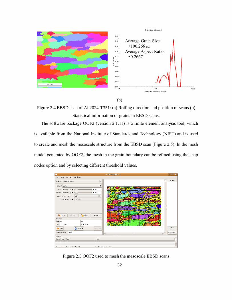
2.4 EBSD Scan of Al 2024-T351: (A) Rolling Direction and Position of Scans (B)
Statistical Information of Grains in EBSD Scans. ............................................................ 32
2.5 OOF2 Used to Mesh the Mesoscale EBSD Scans ...................................................... 32
2.6 Mesoscale RVE Model of Al 2024-T351 ................................................................... 33
2.7 Flattened 3d Polar Plots of Crystal Orientation: A) {1,0,0}; B) {1,1,0}; C) {1,1,1}. 34
2.8 Distribution of Misorientation in Nine SVE Models. ................................................. 35
2.9 Statistical Distribution Used for Misorientation Feature Identification: A) Actual
Data; B) Generated SVE (Model 7). ................................................................................. 36
2.10 Comparison of the SVE Models with Reference SVE: A) Difference vs. Orientation;
B) Average Errors. ............................................................................................................ 37
2.11 SVEs Constructed For Feature Study: A) Baseline; B) Misorientation; C) Principal
Axis Direction; D) Grain Size; E) Aspect Ratio; F) Grain Shape. Feature Effects Could
be Studied Through Comparison of Results with Respect to the Baseline....................... 39
2.12 Variation In Average Plastic Strain Energy Density vs. Time. ................................ 41

viii
Figure Page
2.13 Plastic Strain Energy Density Distributions Within SVEs: A) Baseline; B)
Misorientation; C) Principal Axis Direction; D) Grain Size; E) Aspect Ratio; F) Grain
Shape. ................................................................................................................................ 42
2.14 FEA Model with RVE and SVE at the Same Hot Spot ........................................... 44
2.15 Distribution of Strain Energy Density in RVE Model .............................................. 45
2.16 Distribution of Strain Energy Density in an SVE Model ........................................ 45
2.17 Comparison Between RVE and SVE ....................................................................... 46
2.18 Local Von Mises Stress Field Distribution Within Lug Joint A) with SVE; B)
Without SVE. .................................................................................................................... 47
3.1 SEM Observation of Major Crack and Micro Crack Nucleation: A) Major Crack and
Intermetallic Particles in the Path; B) Micro Crack Incubation in Iron-Rich Particle; C)
Micro Crack Nucleation in Iron-Rich Particles; D) No Micro Crack Nucleation Observed
in Magnesium-Rich Particles. ........................................................................................... 53
3.2 Element Analysis of Damaged Al 2024-T351 Sample Using EDAX Technique: A)
Micro Crack Incubation in Intermetallic Particles Results in Major Crack Growth; B)
Element Mapping of Aluminum; C) Element Mapping of Copper; D) Element Mapping
of Iron; E) Element Mapping of Magnesium. ................................................................... 54
3.3 EDAX Analysis to Identify Element Composition for Intermetallic Particles. ......... 55
3.4 Intermetallic Points Represented in SVE Model. ...................................................... 56

ix
Figure Page
3.5 A) Slip Planes In FCC Unit Cell; B) Two Perpendicular Material Planes Which are
Totally Independent; C) Two Parallel Material Planes Which are Totally Dependent; D)
Two Material Planes With an Arbitrary Degree Which are Partly Dependent................. 59
3.6 Plastic Zone Around the Micro Crack. ....................................................................... 61
3.7 Micro Crack Length Increase Cycle by Cycle in Slip Directions. ............................. 63
3.8 Schematic Procedure of Projection of Micro Cracks to Major Crack. ...................... 64
3.9 Variable Temperature Condition for Thermal Mechanical Fatigue Tests. ................. 66
3.10 Variable Mechanical Load Condition for Thermal Mechanical Fatigue Tests. ........ 66
3.11 Distribution of Damage Accumulation in Slip System {1 1 1} <1 1 0> at (A) Room
Temperature and (B) 200oC. ............................................................................................. 73
3.12 Lug Joint Specimen for Fatigue Test: A) Crack Initiates in the Shoulder of Lug
Joint and B) Geometric Dimension................................................................................... 75
3.13 Experimental Test Frame for Fatigue Loading (MTS Bionix 370.02). ................... 76
3.14 Boundary Conditions and Implementation of a Two-Scale Mesh at the Structural
Hot Spot of an Aluminum Lug Joint................................................................................. 77
3.15 Simulation Results of Probable Crack Direction. .................................................... 78
3.16 FALSTAFF Loading (79 Cycles) ............................................................................ 80
3.17 Cruciform Specimen: A) A Round Hole in Center for Test; B) A 45° Notch at the
Center Hole for Fatigue Test; C) Geometric Dimension of Cruciform; D) Geometric
Dimension of the Center. .................................................................................................. 82
3.18 RMS Model Based Loading (79 Cycles) ................................................................. 83

x
Figure Page
3.19 Distribution of Plastic Strain Energy Density in A) RMS Model After 79 Cycles; B)
FALSTAFF Model After 79 Cycles ................................................................................. 84
3.20 Average Plastic Strain Energy Density in SVE Model for FALSTAFF & RMS
Loading Conditions with a Frequency of 20HZ. .............................................................. 85
3.21 MTS Biaxial Tension-Torsion Test System ............................................................ 86
3.22 Cracks in Experimental Specimens ......................................................................... 87
3.23 Loading Conditions and Implementation of SVE Model at the Structural Notch Tip
of an Al 2024-T351 Cruciform. ........................................................................................ 88
3.24 Dog Bone Specimen for Tensile Test at Different Temperatures: A) Geometric
Dimension and B) Crack Takes Place in the Middle of Dog Bone Specimen. ................ 90
3.25 Instron Material Test Frame 985 with Thermal Chamber. ...................................... 91
3.26 Stress-Strain Relation of Al 2024-T351 at Different Temperatures ........................ 92
3.27 Crack Initiation Takes Place in Shoulders of Lug Joint Specimen in TMF Test. ... 94
4.1 Modeling of Self-Sensing Polymer Materials at the Microscale, Mesoscale, and
Macroscale. ....................................................................................................................... 98
4.2 Schematic of UV-Initiated Cyclobutane Generation and Damage-Induced Cinnamoly
Group Generation.............................................................................................................. 99
4.3 Fluorescence Observation in Self-Sensing Polymer with Increasing Load: A) No
Crack and No Fluorescence Observed; B) Micro Crack and Slight Florescence Intensity;
C) Major Crack And Higher Florescence Intensity. ....................................................... 100

xi
Figure Page
4.4 Components of Self-Sensing Polymer: A) Epoxy Resin, B) Hardener, C) Smart
Material to Form, and D) RVE Model. ........................................................................... 101
4.5 Schematic of Crosslinked Structure of Epoxy Resin and Hardener: A) Molecular
Structure of Epoxy Resin with Two Active Sites; B) Hardener With Five Active Sites; C)
Epoxy Resin and Hardener are Crosslinked to Generate Polymer Structure. Black Solid
Lines Represent Covalent Bonds. ................................................................................... 102
4.6 Statistical Distribution of Crossing-Linking Degrees Based on MD Simulations (N =
500). ................................................................................................................................ 103
4.7 Uniaxial Deformation Test in MD Simulation: A) Tensile Load and B) Compressive
Load of Self-Sensing Polymer. ....................................................................................... 106
4.8 Relationship Between Crosslinking Degrees and A) Tensile Modulus, B)
Compressive Modulus and C) Shear Modulus. .............................................................. 107
4.9 A) Spring-Bead Model; B) Simplified Spring-Bead Model; C) Mechanical Response
of Spring-Bead Models with Different Crosslinking Degrees. ....................................... 110
4.10 Different Arrangements of Spring-Bead Models to Form a: A) 3 Neighbor Based; B)
4 Neighbor Based; C) 6 Neighbor Based; D) 8 Neighbor Based; E) 12 Neighbor Based
Network Model. .............................................................................................................. 112
4.11 The 6, 8, And 12 Neighbor Based Network Models.............................................. 113
4.12 Isotropic Representation of A) 8 Neighbor Based, and B) 12 Neighbor Based
Network Models Corresponding to Stiffness Ratio of Long Spring to Short Spring. .... 115
xii
Figure Page
4.13 Fitting Curves of Modulus as a Function of Spring Stiffness: A) Tensile Modulus;
B) Compressive Modulus; C) Shear Modulus. ............................................................... 120
4.14 Comparison Between MD Simulation and Optimization Results. ......................... 121
4.15 Linear Fitting Curve of Spring Stiffness Based on Optimization Results. ............ 122
4.16 Beads, Springs, and Subzone in 8 Neighbor Based Network Model. .................... 124
5.1 A) Specific Network Model to Study Effect of Degree of Heterogeneity and B)
Spring Stiffness in Subzone A and B of the Network Model 1, 2, 3 and 4. ................... 128
5.2 The Difference in Neighbor Crosslinking Degree Influences the Difference Between
Maximum and Minimum Equivalent Strain in the Network Model. .............................. 129
5.3 Crosslinking Degree Distribution in A) Statistical Network Model and B)
Homogeneous Network Model (Unit: %). ...................................................................... 131
5.4 Equivalent Strain Distribution in A) Statistical Network Model and B) Homogeneous
Network Model. .............................................................................................................. 132
5.5 A) The Probability Distribution of Crosslinking Degree in the Statistical Network
Model, B) Network Model 1, C) Network Model 2, and D) Network Model 3. ............ 136
5.6 Average Equivalent Strain In Three Statistical Network Models v.s. Loading Strain.
......................................................................................................................................... 137
5.7 Simulation of Statistical Network Model Under Biaxial Tensile Load: A)
Crosslinking Degree Distribution in Network Model and B) Distribution of Equivalent
Strain in Network Model. ............................................................................................... 138
5.8 Dimensional Drawing of Dog Bone Specimen for Simulation. ............................... 139

xiii
Figure Page
5.9. Strain Distribution in the Hot Spot Using A) Network Model and B) FE Model. .. 140
5.10 Strain Distribution Within Notched Specimen A) with Network Model and B)
Without Network Model. ................................................................................................ 141
5.11 Fluorescence Observation of Self-Sensing Polymer. A) Integrated Intensity Density
v.s. Loading Strain in Fluorescence Observation, B) Microscopic Images and Detected
Fluorescence of Specimen at 4% Strain, and C) Microscopic Images and Detected
Fluorescence of Specimen at 6% Strain. ......................................................................... 143
5.12 Network Model Based Simulation Results: A) Average Equivalent Strain in
Network Model; and Equivalent Strain Distribution at Different Global Strain at B) 3%,
C) 5%, D) 8%, and E) 10%..............................................................................................147
5.13 Tensile Mechanical Responses of Self-Sensing Polymer at Variable Crosslinking
Degrees Based on the MD Simulation. ........................................................................... 148
5.14 Equivalent Strain Distribution in Statistical Network Model 1 at Different Loading
Strain: A) 5%, B) 8%, C) 10%, and D) 11.2%. .............................................................. 150
5.15. Experimental Results of Tensile Tests. .................................................................. 150

1
1. Introduction
1.1. Motivation
Damage detection, accurate material modeling techniques and structural health
monitoring (SHM) are emerging technologies critical to both current and future
multidisciplinary applications (Carol, 1997; Bond, 2000; Glisic, 2008; Giurgiutiu, 2008;
Farrar, 2006; Mohanty, 2010). The goal of an SHM framework is to detect, quantify, and
classify the nature of damage in a structure in order to assess the current state and
determine the residual useful life (RUL). As a comprehensive technology, SHM
integrates sensors and sensing techniques, damage detection algorithms, and prognosis
for accurate estimation of RUL. A significant amount of research has been conducted in
this field to enhance the fidelity of damage assessment models in metallic materials and
composites (Clayton et al., 2004; Fan et al., 2001; Bakis, 2002; Kadi, 2006; Hochhalter et
al., 2010; Horstemeyer and McDowell, 1998; Sundararaghavan and Zabaras, 2008;
Chattopadhyay et al., 2009). An integrated framework of damage detection that includes
material characterization, multiscale modeling, sensing, prognosis, experimental
validation and information management has been developed by Chattopadhyay et al.
(Chattopadhyay, 2009). However, a general sensing methodology that can be used for
every conceivable damage state in a structure is currently not available. Also, there is a
considerable limitation on the size of detectable damage using off-the-shelf sensors.
Therefore, there is a need for multiscale modeling techniques to understand damage
initiation and track its evolution across the length scales. Information on damage
initiation at the microscale and its manifestation at the macroscale, obtained from the

2
multiscale models, can be combined with physical sensor data to construct a hybrid data
base for damage estimation and detection. The output of this effort can be used in
diagnostics as well as prognostics. Most importantly, multiscale modeling is the key to
understanding precursors to damage.
In this thesis, effort has been dedicated to develop multiscale modeling approaches
and associated damage criteria for the estimation of damage evolution which is essential
to damage detection. Two different materials, aluminum alloy and smart particle
embedded epoxy polymer (which will be discussed in more details in the following
sections) are studied. Important issues, such as length and time scales, variability in
material properties and mechanical behavior at the microscale due to crystallography and
geometry of grains for metal and crosslinked microstructure for polymer, are addressed in
this research. A background of the relevant research is discussed in the following
sections.
1.2. Background of multiscale modeling for metallic material
A broad range of multiscale modeling techniques have been reported in recent
literature using the meso representative volume element (RVE) approach to merge the
length scales (Balzani, 2009; Kanit, 2003; Trias, 2006). Nakamachi (2007) developed a
two-scale homogenization theory to assess the sheet metal formability. A realistic RVE
model was employed for the micro polycrystal structure, which was determined by the
scanning electron microscopy and the electron backscattering diffraction (SEM-EBSD)
measurement. Using this technique, the morphological and crystallographic textures of
the microstructure can be obtained with an accurate spatial resolution. St.-Pierre et al.

3
(2008) developed a new methodology based on Voronoi tessellation to create realistic 3D
microstructures of polycrystalline materials. Experimental inputs from SEM-EBSD
measurements were used to reproduce the grain morphology, including grain boundaries
and the anisotropy of the grain shape. Luo (2009) directly obtained a meso RVE through
microstructure scans of actual material samples containing various differently oriented
grains. The material behavior in hot spots or areas of high stress concentrations was
explicitly modeled using an RVE containing microstructure in order to capture grain size
and orientation effects, while homogenous material properties were used outside the hot
spots. This multiscale model captures anisotropic behavior at the microscale due to
crystalline orientations while maintaining the isotropic material behavior at larger scales
in accordance with the isotropic macroscale material behavior obtained from
experiments. Experiments were implemented using lug joint specimen under uniaxial
fatigue loading and cruciform specimen under biaxial fatigue loading. While this
methodology provides both crack length and direction of crack growth with sufficient
accuracy when compared to experiments, it requires large amounts of experimental data
and associated pre-processing. Also, for accuracy, the material scan has to be acquired
from the same exact location where the RVE is positioned at the structural scale. In
addition, such an approach is deterministic in nature; therefore for a different sample, the
RVE model must be reconstructed based on a new material scan. This is time-consuming,
CPU intensive, and more challenging in applications with limited accessibility. The
shortcoming of the RVE model has been addressed through the development of the
statistical volume element (SVE) model to study polycrystalline microstructures. A

4
considerable amount of research has been reported on SVE models in the context of
stochastic modeling. Groeber (2007, 2008) made significant improvements on
characterization of 3D polycrystalline microstructures and 3D SVE modeling by taking
into consideration grain features, including orientation, misorientation, and grain size in
the generation of an SVE model. SVE models have also been applied in the prediction of
crack initiation and fatigue life. Yin et al. (2008) developed an SVE method to analyze,
quantify, and calibrate microstructure-constitutive property relations using statistical
means. Voids (defects) were randomly generated in their SVE model prior to studying the
material‘s constitutive response. However, the crack incubation and nucleation stages
were not studied in their work. Hochhalter (2010) focused on a comprehensive study of
crack nucleation prediction and growth in grain boundaries. Grain features, including
grain orientation, misorientation, and boundary shape were considered in their model, and
based on their results, it was seen that grain orientation had a significant effect on the
nucleation metrics. Although the focus of their study was on small fatigue cracks (length
in the order of 10 µm), their work could be used in further construction of SVE models
and mesoscale crack prediction (up to 1 mm length). Guilleminot et al. (2011) generated
an SVE model using strain energy density criteria. This SVE model showed a more
accurate response because the construction of the SVE is based on mechanical properties.
However, the geometric features of the material are neglected in their SVE model to
improve simulation efficiency. Therefore, an SVE model based multiscale modeling
approach is required in which both the geometric features and crystallographic features
are taken into account. In addition to capturing statistical effects, the use of SVEs may

5
also reduce preprocessing time and computational effort. The methodology outlined in
this work results in a significant increase in computational efficiency through a
reasonable reduction of elements in the analysis, which is essential for the use of
multiscale models in sensing applications.
Fatigue crack prediction for metallic materials is an important consideration in the
design and maintenance planning of many structural components in aerospace vehicles
(Clayton, 2004; Fan, 2001; Hochhalter, 2010; Horstemeyer, 1998; Sundararaghavan,
2008; James, 1997; Newman, 1999). Extensive research has been conducted over the past
several decades; however, accurate prediction of the fatigue crack remains a challenging
problem. Fatigue crack growth has been characterized to be both multiscale and
stochastic in nature (McDowell, 2011). Experimental studies of material fatigue have
been performed over the last 100 years, including several observations on the multiple
stages of fatigue. To investigate fatigue phenomenon in different stages, Schijve (1967)
divided fatigue life into four stages: micro crack nucleation, micro crack growth, macro
crack growth, and failure. Forsyth (1969) first noted that fatigue cracks usually start at the
surface of a structural component. He argued that major cracks typically start from micro
cracks on crystallographic slip planes in intermetallic particles and gradually grow in a
direction perpendicular to the external applied load. Pearson (1975) compared the
initiation of fatigue cracks and the subsequent growth of very short cracks (0.006mm-
0.5mm) using two types of aluminum alloys, and observed that short tensile cracks first
initiated at the interface between a surface inclusion and the matrix or within an
inclusion. Once formed, the cracks grew into the matrix in directions approximately

6
perpendicular to the applied tensile stress. Chaussumie (2010) states that the phenomenon
of fatigue involves multiple length scales including micro crack nucleation at the
microscale, coalescence of micro cracks at the meso scale, and major crack propagation
at the macro scale. Hochhalter (2010) presented a comprehensive study of micro crack
nucleation and growth in grain boundaries and found that grain orientation had a
significant effect on the nucleation metrics. It should be mentioned that for aluminum
alloy 2024, only large iron bearing particles, Al7Cu2Fe (β-phase) contributed to the crack
nucleation process (Merati, 2005). Mo (2008) studied the phenomena of coalescence of
neighboring micro cracks, formation of larger micro cracks, and subsequent propagation
of a major crack. The cracks in intermetallic particles were considered as micro cracks
that coalesced together and provided a weak path for fatigue crack propagation. Final
fracture occurred when the percentage of cracked particles increased to a threshold level
during the fatigue process. Taylor (2002) studied the behavior of short fatigue cracks at
the microstructural level and proposed that the size of short cracks should be of the same
order of magnitude as the microstructure, typically less than ten grain diameters.
In general there are two major types of modeling methodologies for fatigue crack
prediction: i) a method based on material properties and the damage accumulation rule,
and ii) a method based on fracture mechanics and crack growth analysis, using a physical
approach to damage tolerance analysis. An important drawback of these methods is that
they fail to take into account either the length scale effects or the physical nature of
fatigue. Therefore, it is necessary to develop a length scale dependent and physics-based
model for accurate simulation in order to understand a material‘s performance and
7
ultimately assess the reliability of current aerospace vehicles. Two critical issues need to
be resolved to ensure the viability of such an approach: developing a model that
accurately accounts for the material properties and their variability and a damage
criterion capable of capturing crack initiation and growth. It is important to note that
defects, such as cracks, initiate at the microscale before manifesting at the macroscale
and thus can become a critical factor in final structural failure. As such, prediction of
damage initiation and crack growth can be simulated and verified by applying physics
based multiscale models. To model the nucleation, growth, and coalescence of micro
cracks in complex metallic microstructures, multiscale analysis techniques have been
proposed. A realistic treatment of length scale effects on damage evolution, for instance,
is becoming feasible now when sufficiently sophisticated constitutive laws are used.
Tekoglu (2010) modeled the void nucleation by integrating a damage model with a Mori–
Tanaka type mean-field homogenization scheme that explicitly accounts for the per-phase
behavior. Sun (2008) developed a multiscale continuum model to study the effect of grain
size on the macroscopic dissipative response during isothermal thermoelastic phase
transition. Groh (2009) proposed a numerical, hierarchical multiscale modeling
methodology involving two distinct bridges over nano, micro, and meso scales that
predicts the work hardening of face-centered cubic crystals in the absence of physical
experiments. In order to study the length scale effects on fatigue crack growth, it is
necessary to take into account crystal dislocation mechanics, material microstructure, and
macro scale behavior in the continuum description of finite strain plasticity. Crystal
dislocation provides an atomistic interpretation of the slip process and strain hardening of

8
metals. Jiang (2000) developed a three-dimensional fatigue damage criterion under
multiaxial, non-proportional loading. The effect of grain orientations in fatigue damage
was investigated by Kalnaus (2006). He proposed a damage criterion on a critical slip
plane for single crystalline microstructures. Luo (2011) extended Jiang and Kalnaus‘s
fatigue damage criterion to polycrystalline materials. Aluminum alloy 2024-T351 was
studied in his work. A multiscale model was constructed that linked the relationship
between the damage criteria at the microscale to the crack initiation at the mesoscale. The
multiscale model with fatigue damage criteria initiated at the microscale and the effects
of grain orientation, shape and size were included through material characterization and
crystal plasticity based constitutive relation. It must be noted that the microstructure in
such approaches is generated by using single crystal plasticity theory which neglects
defects such as intermetallic particles within and between grains. Thus, a damage
estimation approach considering both crystal dislocation mechanics and micro crack
nucleation in intermetallic particles is required.
In this dissertation, a multiscale modeling approach is developed for aluminum alloy
(Al 2024-T351). The research starts with material characterization to incorporate
statistical microstructural features. The effects of grain features including orientation,
misorientation and size on the damage evolution are studied in detail and a
microstructural database is created. The SVE model is developed based on this
microstructural database. Details on material characterization, construction of statistical
database, development and parametric study of the SVE model are discussed in the
chapter 2. A physics-based multiscale damage criterion is developed to capture the crack

9
initiation at the microscale and growth at the mesoscale. This criterion is energy based
since the damage index is directly related to the plastic strain energy density. The
derivation of the multiscale fatigue damage criterion and some applications of this
damage model for different structural components and load conditions are presented in
the chapter 3.

10
1.3. Background of multiscale modeling for self-sensing polymer material
Interest in stimuli-responsive materials that exhibit specific chemical reactions upon
external stimuli such as temperature, pH, ion, light, and electric field has increased
significantly in the last twenty years (Suzuki, 1996; Qiu, 2001; Richter, 2008; Bawa,
2009; Tanaka, 2012). Particularly of interest are stress-sensitive materials responsive to
mechanical loading (also known as mechanophores), which open novel ways to study
post-yield behavior at material level (Chang, 1987; Thostenson, 2006; Wu, 2008). Cho
and Chung (Cho, 2010; Chung, 2004) developed a cyclobutane based mechanophore
consisting of carbon-carbon covalent bonds. Under mechanical loading, the cyclobutane
transforms into cinnamate groups, which emit green fluorescence. Zou et al. (2014)
developed a novel self-sensing technique by embedding the Tris-(Cinnamoyl
oxymethyl)-Ethane (TCE) as the cyclobutane-based self-sensing material in polymer
matrix. They incorporated the cyclobutane-containing crosslinked polymers into an
epoxy matrix, studied the effect on mechanical properties and demonstrated early damage
detection through mechanically induced fluorescence. The experimental research has
shown significant promise in developing mechanophore embedded polymer materials
which can be used to detect damage initiation in polymeric composite materials (Zou,
2014). Previous studies have reported the experimental characterization and fabrication
of nanoparticle-embedded polymers (Gibson, 2010). However, the determination of
mechanical properties through testing is labor intensive and expensive. Modeling
techniques are now necessary to simulate the multiscale response of these ―smart‖
polymers.

11
In epoxy based polymers the crosslinked bond clusters between the resin and the
hardener molecules generate a larger scale of network structure. The heterogeneous
crosslinked network at the microscale has significant effect on the local mechanical
properties (Flory, 1943; Krumova, 2000; Fan, 2007). Therefore to design and synthesize
polymers with multifunctional capabilities it is important to develop a fundamental
understanding of the effects of microscale variability on material properties and response
such as Young‘s modulus, heterogeneous stress/strain distribution and damage initiation.
Numerous approaches have been developed to model polymeric systems integrated with
nanoparticles. These include homogenization techniques, finite element (FE) method,
molecular dynamics (MD) simulation, Monte Carlo (MC) simulation, and the Mori-
Tanaka approach (Ghosh, 1995; Borodin, 2005; Fermeglia, 2007). Among these
techniques the MD model and FE model are two of the most widely used methods to
understand the material behavior of epoxy based systems at the nanoscale and
microscale. The heterogeneous material properties of polymer, which is influenced
significantly by crosslinking degree, can be effectively captured by MD simulation
(Flory, 1943; Fan, 2007; Krumova, 2000). Fan et al. (2000) performed MD simulations to
characterize the material properties of the crosslinked epoxy resin compound. Linear
thermal expansion coefficients and Young's modulus of the material can be captured
using their model. Yarovsky and Evans (Yarovsky, 2002) investigated the strength and
molecular mechanisms of adhesion between an inorganic substrate and a cured epoxy
resin using MD simulation. In their model, the crosslink density and corresponding
material properties of the crosslinked system were successfully estimated. However, the

12
significantly high computational cost associated with large-scale MD simulations is a
major hurdle and often limits its application beyond the nanoscale. The FE model is
computationally efficient and can capture the material performance of polymers. Onck et
al. (2005) developed a two-dimensional model to study the strain stiffening of
crosslinked filamentous polymer. In their work the FE method was used to discretize the
filament with Euler-Bernoulli beam elements accounting for stretching and bending.
Jiang et al. (2007) performed a parametric study using FE analysis to compute the
material properties and scratch behavior of crosslinked polymer. Their simulation results
correspond well with the mechanical properties obtained from experiment. Chen and
Lagoudas (2008) developed a constitutive theory for polymers in which the crosslinking
density is considered to influence the mechanical behavior. Their model was
implemented and extended using FE method by other researchers to study
thermoelasticity, viscoelasticity and nonequilibrium relaxation (Westbrook, 2011; Volk,
2010; Diani, 2012). However, the FE method cannot be used to model heterogeneous
microstructure because the definition of discontinuous material properties is often
infeasible in FE approach. Therefore, new techniques with improved computational
efficiency and high accuracy are desired for investigating the material behavior of
polymers at the microscale.
Discrete material techniques, such as the spring-bead model, have been developed to
study polymer material (Buxton, 2002; Iwata, 2003; Schwarz, 2006). Underhill and
Doyle (2005) developed a new method for generating coarse-grained models of
polymers. The spring-bead chains were further crosslinked to generate a network model

13
to represent the larger scale material behavior of polymer (Indei, 2012).A spring-bead
based network model, which bridges nanoscale information to higher length scales, was
developed by the authors (Zhang et al., 2014) to model this class of epoxy polymers
embedded with TCE monomer. The material was partitioned into discrete mass beads
which were linked using linear springs at the microscale. By integrating multiple spring-
bead models a network model was constructed to represent the material properties at the
mesoscale. A series of MD simulations were performed initially to define the spring
stiffness in the statistical network model. Compared with the MD model, only the
equivalent mechanical responses which influence the damage initiation significantly was
captured in the spring-bead based network model. The other material properties, such as
the thermal properties and chemical properties were neglected to improve simulation
efficiency. The developed multiscale methodology was computationally efficient and it
was able to provide a possible means to bridge various length scales (from 10 nm in MD
simulation to 10 mm in FE model) without significant loss of accuracy. In this work, the
statistical network model is further investigated to understand the effects of the model
parameters on material response and damage in the TCE embedded polymer. The model
is also used to develop a relationship between mechanical strain and experimentally
observed fluorescence, with damage growth, in the self-sensing polymer under multiaxial
loading.
The parameters in the crosslinked network model (such as the crosslinking degree,
chain flexibility and chain length) affect the material performance (Espuche, 1995;
Chzarulatha, 2003; Park, 2006). These effects were studied by observing their mechanical

14
properties. Among all variability, the crosslinking degree which represents the degree of
microscopic crosslinked covalent bonds was shown to have a more significant effect on
the mechanical properties (Zosel, 1993; Espuche, 1995; Halary, 2000; Berger, 2004).
Urbaczewski-Espuche et al. (1991) developed a crosslinked network model and studied
the influence of the crosslinking degree on the mechanical properties of epoxy. The
results showed that the mechanical properties including Young‘s modulus, ultrasonic
modulus, thermomechanical relaxation, and plastic behaviors are affected by crosslinking
degree. Svaneborg et al. (2005) investigated the effect of microscopic disorder on the
mechanical response of network models of the same crosslinking degree. They concluded
that the heterogeneities in the randomly generated crosslinked network models cause
significant differences in the localization of monomers. Parametric study through the
developed network model can help to understand the self-sensing polymeric material‘s
microscopic performance.
In this dissertation, a spring-bead based network model is developed to bridge
nanoscale information to higher length scales for modeling epoxy polymers embedded
with smart particles. A series of MD simulations are performed to capture the generation
of crosslinked bonds in the self-sensing polymer; this information is further used to
construct the probability distribution of crosslinking degrees. Mechanical equivalence
optimization was implemented to bridge the mechanical properties between the MD
system and the network model. The MD simulation results, details of the spring-bead
model, network model, and mechanical equivalence optimization are discussed in chapter
4. Parametric study based on the developed statistical network model is performed to
15
understand the influence of design variables on material behavior. A series of simulations
are performed to compare the effects of the crosslinking degree on the strain distribution.
The knowledge obtained is important to the enhancement of the material performance by
controlling the crosslinking degree during the manufacturing process. Experiments were
conducted to validate the network model. The average equivalent strain of network model
is used to capture the fluorescence intensity of the self-sensing material. A physics based
damage evolution is developed to estimate the damage evolution. The parametric study,
validation and damage evolution of the network model are presented in chapter 5.
1.4. Objectives
Multiscale modeling of Al 2024-T351
A multiscale modeling framework is developed, which includes characterization of
microstructural features and variability, development of a meso SVE model to represent
the material behavior, development of a physics-based damage criterion, and
experimental validation to predict the fatigue life of Al 2024-T351. The key objectives of
this research are as follows.
1) Characterize microstructural material properties including grain features and
intermetallic particle features to construct a statistical data base;
2) Implement parametric studies of grain features including grain orientation,
misorientation, grain size, grain shape, aspect ratio and principal axis direction to
assess the sensitivity of each parameter;
3) Develop a meso SVE model to represent the material properties and perform
validation through RVE based simulation;

16
4) Develop a physics based multiscale damage criterion to predict fatigue life and
crack direction in Al 2024-T351 based complex structural components. Two
important stages of the crack initiation are modeled: micro crack nucleation and
major crack formation;
5) Modify the physics based multiscale damage criterion to predict crack formation
in thermo-mechanical fatigue (TMF) loading;
6) Perform damage analysis using the multiscale model and the damage criterion in
lug joints under uniaxial fatigue loading, cruciform specimen under biaxial
fatigue loading and lug joints under uniaxial TMF loading.
Multiscale modeling of a self-sensing polymer material
A spring-bead based network model is developed to model the mechanical properties
of a novel mechanophore crosslinked polymer which is capable of detecting damage
precursor. The modeling framework includes mechanical equivalence optimization based
on properties obtained from MD simulations, parametric studies of microscopic
variability, experimental validation and estimation of damage precursor in polymeric
material based on MD simulation and network model. The present multiscale modeling
work of the self-sensing polymer material addresses the following objectives.
1) Develop a spring-bead based network model to represent the mechanical
properties of self-sensing polymer material; simulate the mechanical response of
the crosslinked springs in the network model using statistical material behavior
obtained from MD simulation;

17
2) Conduct configuration analyses and mechanical equivalence optimization to
construct the optimal arrangement of the network model;
3) Perform parametric studies of the network model to understand the influence of
design variables such as distribution of crosslinking degree and spring length on
material behavior;
4) Validate the mechanical properties of the spring-bead based network model
through experiments;
5) Capture the self-sensing fluorescence intensity observed in experiment through
the network model based simulation;
6) Evaluate the damage evolution using a strain based index based on MD
simulation and network model.
1.5. Outline of the dissertation
The dissertation is structured as follows. Six chapters are presented.
Chapter 2 provides an introduction of single crystal plasticity theory which is used to
capture the crystallographic and geometric effects of grains at the microscale. A
subroutine UMAT is introduced to incorporate the single crystal plasticity in the FEA
program. Material characterization procedures from Electron Backscattering Diffraction
(EBSD) scans are discussed. Development of an SVE model based on the statistical
features of material at the microscale is presented. A parametric study is performed to
assess the sensitivity of grain features. The SVE model is validated through comparative
simulations using an RVE based model.
18
Chapter 3 presents studies on material characterization and microstructure
investigations. The microstructural features of intermetallic particles are obtained from
scanning electron microscope (SEM) and energy dispersive X-ray microanalysis
(EDAX). The development of a multiscale physics damage criterion is discussed. The
damage criterion is further modified to capture damage initiation under TMF loading.
Details of simulation results and experimental validations are discussed.
Chapter 4 presents a multiscale framework to represent a self-sensing polymer
material. Self-sensing behavior of the smart material and atomistic scale studies using
MD simulation are introduced. Development of a spring-bead based network model,
analyses of different combination arrangements of springs and beads in network model
and mechanical equivalence optimization are discussed. Definition of equivalent strain
and strain energy density in the network model is also introduced at the end of this
chapter.
Chapter 5 presents the parametric studies conducted using the network model to
understand the influence of microscopic variability on material behavior. The
development of a statistical network model is presented. Validation of the network model
is performed through experiments and FE simulations. Correlation between fluorescence
intensity observed in experiments and average equivalent strain in the network model
based simulation is presented. The development of a strain based damage evaluation
approach to estimate the damage evolution based on MD simulation and network model
is also introduced.

19
Chapter 6 summarizes the research work reported in this thesis, and emphasizes the
important original contributions and findings of this dissertation. Suggestions on future
research directions and recommendations are also discussed at the end of this chapter.

20
2. Material Characterization and Multiscale
Modeling of Aluminum Alloy 2024-T351
2.1. Introduction
A broad range of multiscale modeling techniques have been reported in previous
research and within these, the meso representative volume element (RVE) approach is a
popular technique. The RVE model is directly obtained through microstructure scans of
actual material samples containing various differently oriented grains. While this type of
approach has qualified accuracy, it requires large amounts of experimental data and
associated pre-processing. Also, for accuracy, the material scan has to be acquired from
the same exact location where the RVE is positioned. In addition, such an approach is
deterministic in nature; therefore for a different sample, the RVE model must be
reconstructed based on a new material scan. This is time consuming, CPU intensive, and
more challenging in applications with limited accessibility.
The statistical volume element (SVE) methodology for multiscale analysis and
fatigue life prediction is outlined in this section. The primary goal of this research is to
improve the computational efficiency and reduce the preprocessing effort associated
while maintaining accuracy. Simplified grain shapes are employed because they offer
ease of assembly, reduced preprocessing time, and reduced total number of elements used
(irregular grain shapes result in small features, thereby requiring a large number of small
elements). Using the SVE methodology, grains with features that are statistically sampled
from pools of measured experimental characterization data are assembled, as shown in

21
Figure 2.1(b). This approach provides a computationally efficient alternative to
traditional techniques while maintaining statistical accuracy.
a) b)
Figure 2.1 Comparison between: a) actual microstructure scans; b) constructed SVE.
Colors represent different grain orientations.
To capture the crystallographic effect of grains at the microscale, single crystal
plasticity is introduced. This is then incorporated into the commercial finite element (FE)
program ABAQUS (version 6.10.1) with the help of a user material (UMAT) subroutine.
Material characterization, including Electron Backscattering Diffraction (EBSD) scans
and OOF2 (Object-Oriented Finite) meshing are implemented to capture the geometric
and crystallographic features of grains. Representative volume element (RVE) and SVE
models are developed to demonstrate material properties and mechanical responses
occurring at the mesoscale. Finally, a series of simulation validations is performed. The
results show that the SVE model is capable of representing the bulk material and
mechanical responses of the polycrystalline material.

22
2.2. Single crystal plasticity theory
To study the mechanical properties of aluminum alloy 2024-T351, which is face
centered cubic (FCC) crystalline structure, the single crystal plasticity theory is
introduced to capture the crystallographic orientation effects on polycrystalline material.
The kinematic theory for single crystal deformation in this research is based on the
pioneering works of Taylor (1938), Hill (1966), Rice (1971), and Asaro (1983). In these
works, the deformation gradient, , is decomposed into elastic and plastic
components under standard multiplicative decomposition assumption (Figure 2.2 and
Equation 2.1) as follows:
Figure 2.2 Multiplicative decomposition of deformation gradient (Luo, 2009)
(2.1)
where Fp represents plastic deformation of the material in an intermediate configuration
in which the lattice orientation and spacing remain the same as in the reference
configuration. Fe represents elastic component of the deformation gradient, which
23
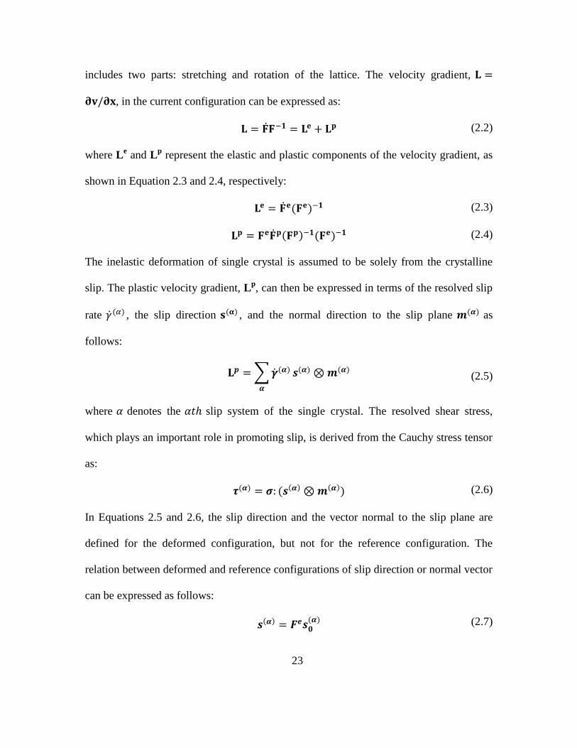
includes two parts: stretching and rotation of the lattice. The velocity gradient,
, in the current configuration can be expressed as:
(2.2)
where Le and L
p represent the elastic and plastic components of the velocity gradient, as
shown in Equation 2.3 and 2.4, respectively:
(2.3)
(2.4)
The inelastic deformation of single crystal is assumed to be solely from the crystalline
slip. The plastic velocity gradient, Lp, can then be expressed in terms of the resolved slip
rate , the slip direction , and the normal direction to the slip plane as
follows:
∑
(2.5)
where denotes the slip system of the single crystal. The resolved shear stress,
which plays an important role in promoting slip, is derived from the Cauchy stress tensor
as:
(2.6)
In Equations 2.5 and 2.6, the slip direction and the vector normal to the slip plane are
defined for the deformed configuration, but not for the reference configuration. The
relation between deformed and reference configurations of slip direction or normal vector
can be expressed as follows:
(2.7)

24
(2.8)
The velocity gradient in the current state can be decomposed into the symmetric rates of
stretching tensor D and anti-symmetric spin tensor Ω in Equation 2.9:
(2.9)
The stretching and spin tensor can be further decomposed into lattice and plastic parts,
respectively:
(2.10)
(2.11)
From Equations 2.3 and 2.5, the Equations 2.10 and 2.11 can be further expressed as
follows:
(2.12)
∑
(2.13)
Following the methodology developed by Hill and Rice (Hill, 1966; Rice, 1971; Hill and
Rice, 1972), the relation between stretching tensor and the Jaumann rate of Cauchy stress
is as follows:
( ) (2.14)
Based on the work of Horstemeyer and McDowell (1998, 1999), a power law is used in
the flow rule to calculate the slip increment in polycrystal elastoplasticity as follows:
|
|
(2.15)

25
where and represent the shear strain rate and shear stress on the slip system,
n is the strain rate exponent parameter, and and represent the isotropic and
kinematic hardening, respectively. The hardening law for and are as follows
(Huang, 1991):
∑
(2.16)
| | (2.17)
where {
|
|
are called self and latent hardening
moduli, respectively. Here, b, r, and q are material constants, h0 is initial hardening
modulus, τs is the stage I stress, and τ0 is yield stress. The cumulative shear strain of all
slip systems in the polycrystalline materials can be obtained as follows:
∑∫ | |
(2.18)
More details of hardening theory for crystalline materials can be found in Asaro and
Peirce (Asaro, 1983; Peirce et al, 1982).
2.3. User defined material subroutine
In this multiscale modeling approach, a UMAT subroutine based on Huang‘s single
crystal plasticity theory (Huang, 1992) is used. Luo (2009) and Zhang (2012) modified
the UMAT subroutine and add a developed damage criterion to evaluate microscale
damage initiation and growth. In their work, the UMAT subroutine was used to
incorporate single crystal plasticity in the finite element program ABAQUS. The finite
element formulation of elastic-plastic and viscoplastic single crystal deformation was

26
taken into account, including versions for small deformation theory and for a rigorous
theory of finite strain and finite rotation. Inelastic deformation of a single crystal occurs
as a result of crystalline slip, which is assumed to obey Schmid‘s law (Asaro, 1979).
Various self and latent hardening relations between resolved shear stress and shear strain
in slip systems are presented and incorporated as options in the subroutine. An option of
using the linearized solution procedure and evaluating the stress and solution dependent
state variables at the start of the time increment (time t), or using the Newton-Rhapson
iterative method to solve the nonlinear increment and evaluating the stress and solution
dependent state at the end of the time increment ( ∆ ) is provided.
In this research, the polycrystalline material Al 2024-T351, in which the orientations
of grains change from one grain to another, is approached. To account for the arbitrary
crystal orientations, two coordinate systems, global coordinate system for specimen and
local coordinate system for crystalline are applied in the simulation. The global
coordinate system is fixed to the reference configuration while the local coordinate
system is aligned with the crystal lattice. At the beginning of each time increment, the
global strain increment, the time increment, global stress, and the solution-dependent
state variables are given to the subroutine from the main program in ABAQUS. The
subroutine UMAT is used to transform the global strain increment and stress into the
local system. In the local coordinate system, the incremental stress is computed based on
single crystal plasticity theory (Huang, 1993) and transformed into the global system. At
the end of each incremental step, the stress and state variables are updated for use in the
main program in ABAQUS. Then, the next load increment is applied and a new strain

27
increment is generated. This loop is repeated until computation at all incremental time
steps is completed.
The subroutine UMAT is written for cubic crystals. The subroutine can accept, as
input, up to three sets of slip systems for each cubic crystal. There is observation of the
activation of slip system {1 1 0}<1 1 1>, {1 2 1}<1 1 1>, and {1 2 3}<1 1 1> in BCC
metal crystals, and {1 1 1}<1 1 0> in FCC metal crystals. There are seven user supplied
function subprograms, F, DFDX, HSELF, HLATNT, GSLP0, DHSELF, and DHLATN in
the main subroutine UMAT. These characterize the crystalline slip and hardening of slip
systems. The function subprogram F provides the slipping rate , as shown in
Equation 2.15 at the start of the increment, while function subprogram DFDX gives its
derivative as
. The function subprograms, HSELF and HLATNT, provide the
self and latent hardening moduli defined in the incremental formulation (Equation 2.16).
The function subprogram GSLP0 provides the initial value of the current strength
,
and its default is the yield stress . The function subprograms, including DHSELF and
DHLATN, necessary only when the Newton-Rhapson iterative method is used, provide
the derivative of self and latent hardening moduli.
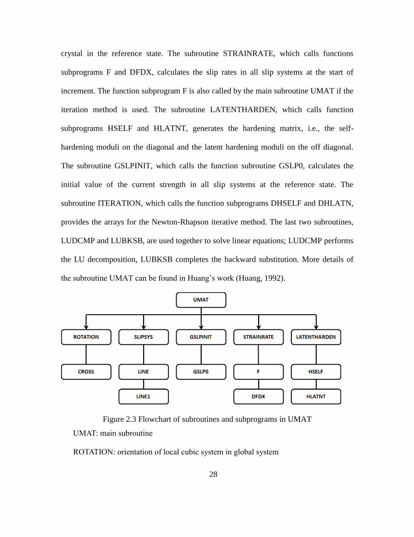
There are eight subroutines, ROTATION, SLIPSYS, STRAINRATE, GSLPINIT,
LATENTHARDEN, ITERATION, LUDCMP, and LUBKSB in the main subroutine
UMAT. The relation of the first five subroutines with the main subroutine UMAT and
function subprograms are shown in figure 2.3. The subroutine ROTATION determines
the initial orientation of a cubic crystal in the global system, while SLIPSYS generates all
slip systems (slip directions and normal to the slip planes) in the same set for a cubic
28
crystal in the reference state. The subroutine STRAINRATE, which calls functions
subprograms F and DFDX, calculates the slip rates in all slip systems at the start of
increment. The function subprogram F is also called by the main subroutine UMAT if the
iteration method is used. The subroutine LATENTHARDEN, which calls function
subprograms HSELF and HLATNT, generates the hardening matrix, i.e., the self-
hardening moduli on the diagonal and the latent hardening moduli on the off diagonal.
The subroutine GSLPINIT, which calls the function subroutine GSLP0, calculates the
initial value of the current strength in all slip systems at the reference state. The
subroutine ITERATION, which calls the function subprograms DHSELF and DHLATN,
provides the arrays for the Newton-Rhapson iterative method. The last two subroutines,
LUDCMP and LUBKSB, are used together to solve linear equations; LUDCMP performs
the LU decomposition, LUBKSB completes the backward substitution. More details of
the subroutine UMAT can be found in Huang‘s work (Huang, 1992).
Figure 2.3 Flowchart of subroutines and subprograms in UMAT
UMAT: main subroutine
ROTATION: orientation of local cubic system in global system

29
CROSS: cross product of two vectors
SLIPSYS: generating all slip systems
LINE: [mmm] type of slip systems
LINE1: [0mn] type of slip systems
GSLPINIT: initial values of current strain hardening functions in all slip systems
GSLP0: user supplied functional subroutine for the initial value in each system
STRAINRATE: shear strain rate in all slip systems
F: user supplied functional subroutines for the shear strain rate in each slip system
DFDX: user supplied functional subroutine for the derivative of function F
LATENTHARDEN: hardening matrix
HSELF: user supplied functional subroutine for the self-hardening modulus
HLATNT: user supplied functional subroutine for the latent hardening modulus
2.4. Material characterization
The material used in this research is aluminum alloy 2024-T351. Relevant material
compositions and properties are shown in Table 2.1 and Table 2.2. To capture the
mechanical response of the polycrystalline material at the mesoscale, a RVE model is
required to characterize the geometric and crystallographic properties of the grains. The
mesoscale model is constructed based on the microscale scans, which contain 2,127
grains, which is sufficient to construct an RVE model. In the RVE model, each grain has
a single crystal structure.
Table 2.1 Specified Composition for 2024-T351 (wt%) (Bussu, 2003)
Element Cu Mg Mn Fe Si Zr Cr Ni Pb Sn Al
2024- 3.8- 1.2- 0.3- 0.5 0.5 0.2 0.1 0.05 0.05 0.05 Rem

30
T351 4.9 1.8 0.9

31
Table 2.2 Mechanical and Physical Properties of 2024-T351 at Room Temperature
(Rodopoulos, 2004)
Elastic modulus (GPa) 72-74 Hardness (HB) 115-120
Shear modulus (GPa) 27-28 Fr. toughness (MPa·m1/2
) 31-34
Poisson's ratio 0.33 Ult. tensile strength (MPa) 490-520
Mon. yield stress (MPa) 325-340 Endurance limit (MPa, R=-1) 135-140
Cyclic yield stress (MPa) 420-450 Shear strength (MPa) 285-301
The first step of material characterization is to take a number of EBSD scans (Figure
2.4) from which are obtained the crystal orientation and geometric properties of each
grain. In the EBSD scans, in which grains are represented by various colors, it is obvious
that the grain features are affected by the rolling direction in the material manufacturing.
The principal axis direction of grain, for example, slants towards the rolling direction (as
shown in Figure 2.4a).
(a)
32
(b)
Figure 2.4 EBSD scan of Al 2024-T351: (a) Rolling direction and position of scans (b)
Statistical information of grains in EBSD scans.
The software package OOF2 (version 2.1.11) is a finite element analysis tool, which
is available from the National Institute of Standards and Technology (NIST) and is used
to create and mesh the mesoscale structure from the EBSD scan (Figure 2.5). In the mesh
model generated by OOF2, the mesh in the grain boundary can be refined using the snap
nodes option and by selecting different threshold values.
Figure 2.5 OOF2 used to mesh the mesoscale EBSD scans

33
Finally, the geometric and crystallographic properties obtained from EBSD are
assigned to the grains to generate the meso RVE model using the commercial FEA
software ABAQUS and the previously developed UMAT subroutine (Figure 2.6). The
RVE model is used to bridge the crystalline grain microstructure at the microscale to the
structural response of a component at the macroscale.
Figure 2.6 Mesoscale RVE model of Al 2024-T351
2.5. Feature parametric study
Figure 2.7 shows three pole figures for grain orientations. The distributions do not
exhibit any trends, and therefore, are assumed to be normally distributed. It must be noted
that when formulating the SVE, the orientations were chosen at random from the pool of
available material characterization data. The misorientations between neighbor grains
were determined from the arrangement of the grains in the SVE. To accomplish this, nine
randomly orientated SVEs were generated (Figure 2.8). A typical histogram of their
misorientation is shown in Figure 2.8 (a)-(i). The misorientation was chosen to closely
match that of the experimental data (Figure 2.9). The difference, i.e., the error between
the randomly generated SVEs and the experimental data, is shown in Figure 2.10. The

34
seventh generated SVE is the closest match to the experimental data, and therefore, was
used in this analysis.
(a) (b) (c)
Figure 2.7 Flattened 3D polar plots of crystal orientation: a) {1,0,0}; b) {1,1,0}; c)
{1,1,1}.
a) Model 1 b) Model 2

35
c) Model 3 d) Model 4
e) Model 5 f) Model 6
g) Model 7 h) Model 8
i) Model 9
Figure 2.8 Distribution of misorientation in nine SVE models.
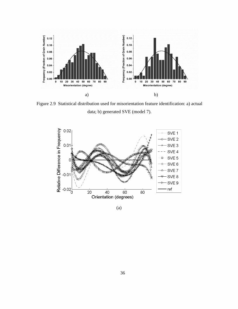
36
a) b)
(a)
Figure 2.9 Statistical distribution used for misorientation feature identification: a) actual
data; b) generated SVE (model 7).

37
(b)
Figure 2.10 Comparison of the SVE models with reference SVE: a) difference vs.
orientation; b) average errors.
To understand the effects and sensitivity of each feature used in the SVE formulation,
several parametric studies were conducted. The features considered in this study were
grain orientation, misorientation (Groeber, 2007; Wang, 2009), principal axis direction,
size, aspect ratio, and shape. In order to create an optimal SVE, each feature has to be
represented by an appropriate statistical observation. However, this process can be
complex and time consuming. In this work, only grain orientation was chosen as a
statistical feature because it is a primary factor in single crystal plasticity that results in
damage initiation (Asaro, 1977; Hill, 1966; Hochhalter, 2010). Experimental observation
has shown that this data is randomly distributed. The remaining features, except
misorientation, are geometric features and can be implemented as a constant value based
on the average experimental observation. To validate this assumption, a feature study was
performed to evaluate the effect of each geometric feature.
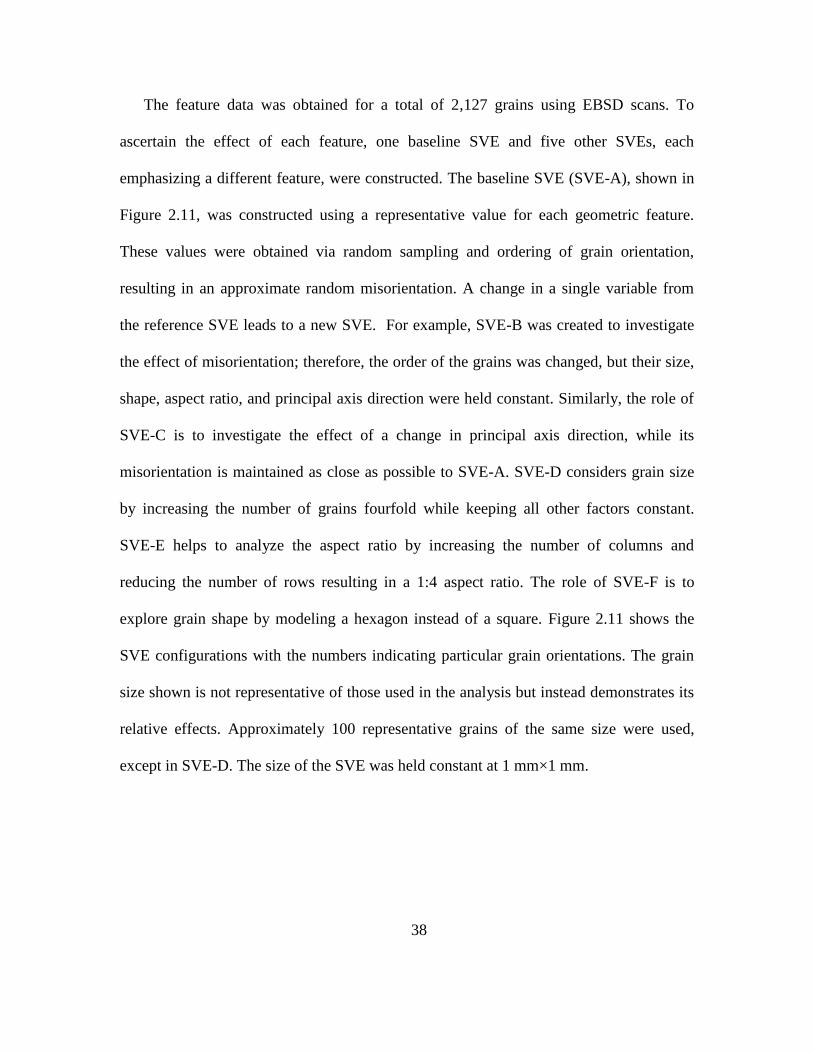
38
The feature data was obtained for a total of 2,127 grains using EBSD scans. To
ascertain the effect of each feature, one baseline SVE and five other SVEs, each
emphasizing a different feature, were constructed. The baseline SVE (SVE-A), shown in
Figure 2.11, was constructed using a representative value for each geometric feature.
These values were obtained via random sampling and ordering of grain orientation,
resulting in an approximate random misorientation. A change in a single variable from
the reference SVE leads to a new SVE. For example, SVE-B was created to investigate
the effect of misorientation; therefore, the order of the grains was changed, but their size,
shape, aspect ratio, and principal axis direction were held constant. Similarly, the role of
SVE-C is to investigate the effect of a change in principal axis direction, while its
misorientation is maintained as close as possible to SVE-A. SVE-D considers grain size
by increasing the number of grains fourfold while keeping all other factors constant.
SVE-E helps to analyze the aspect ratio by increasing the number of columns and
reducing the number of rows resulting in a 1:4 aspect ratio. The role of SVE-F is to
explore grain shape by modeling a hexagon instead of a square. Figure 2.11 shows the
SVE configurations with the numbers indicating particular grain orientations. The grain
size shown is not representative of those used in the analysis but instead demonstrates its
relative effects. Approximately 100 representative grains of the same size were used,
except in SVE-D. The size of the SVE was held constant at 1 mm×1 mm.

39
a) SVE-A b) SVE-B
c) SVE-C d) SVE-D
e) SVE-E f) SVE-F
Figure 2.11 SVEs constructed for feature study: a) baseline; b) misorientation; c)
principal axis direction; d) grain size; e) aspect ratio; f) grain shape. Feature effects could
be studied through comparison of results with respect to the baseline.
Each SVE was analyzed by performing a multiscale analysis. A cyclic tensile loading
(489 N-4890 N) was used and the local plastic strain energy densities within the SVEs
were compared. Figure 2.12 shows the average plastic strain energy density of all six
SVEs with respect to time for the first loading cycle. Based on the work by Huang (1992)

40
and Jiang (2000) it is clear that the damage is influenced greatly by accumulation of
plastic strain energy. They have shown that the plastic strain energy increases with
loading time and reaches the maximum value at the end of the loading history; therefore,
the SVEs were compared at this point. The difference between SVE-A and SVE-C was
2.90% and between SVE-A and SVE-E was 0.01%, shown in Table 2.3. Figure 2.13
shows the local plastic strain energy density fields within each SVE. The distributions of
plastic strain energy density in all the SVEs are similar. Additionally, for different SVEs,
the maximum local plastic strain energy densities appear at the right edge of the SVE.
Some interesting observations can be made from these results. The highest average
density appears in SVE-C, but the highest local maximum density appears in SVE-F. The
lowest average density appears in SVE-A, but the lowest local maximum density appears
in SVE-B. This shows that the plastic strain energy density is variable for different points
in the SVE model and that it is a local value. Based on the performed simulations, this
implies that the effect of these factors may be a local phenomenon, not a global one. It
must be noted that the damage initiation criteria depends on the response of the SVE as a
whole and not on the response of a single grain (Horstemeyer and McDowell, 1998;
Ghosh, 2011); therefore the overall effect, considering all grains, is more appropriate in
life prediction. Based on the results, the average difference in plastic strain energy
densities is small when compared to the variability in experimental data, and therefore
each feature can be effectively represented by its average value.
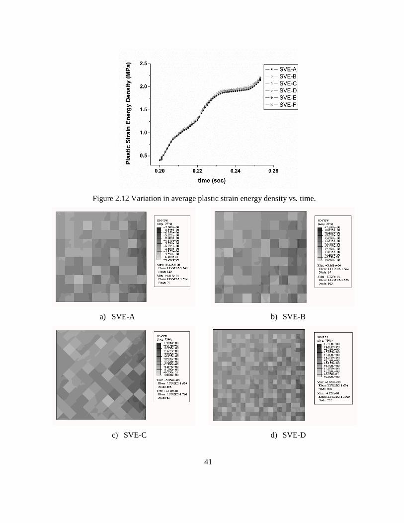
41
Figure 2.12 Variation in average plastic strain energy density vs. time.
a) SVE-A b) SVE-B
c) SVE-C d) SVE-D

42
e) SVE-E f) SVE-F
Figure 2.13 Plastic strain energy density distributions within SVEs: a) baseline; b)
misorientation; c) principal axis direction; d) grain size; e) aspect ratio; f) grain shape.
Table 2.3 Summarized SVE Feature Values
Features Misorientation Principal
axis direction
Grain
size
Aspect
ratio
Grain
shape
Average percent
difference 1.70% 2.90% 0.30% 0.01% 1.80%
The SVE model is constructed by assembling grains whose features are statistically
sampled from pools of measured experimental characterization data. This approach
provides a computationally efficient alternative to traditional techniques while
maintaining statistical accuracy. The non-statistical parameters, including grain size,
shape, aspect ratio, and principal axis direction, were carefully chosen to be
representative of the average response of the material. The gain size was chosen to be
0.025 mm2, while the measured average value was 0.0225mm
2. This is to ensure that an
exact number of grains fit within a 1 mm by 1 mm square SVE. A rectangular grain shape
is used to efficiently assemble the grains within the square SVE. The aspect ratio was
chosen to be 0.4, while the average measured value was 0.384, for the same reason as

43
previously stated. Finally, the principal axis direction was chosen to align with the rolling
direction. The final architecture of the SVE can be seen in Figure 2.1(b). As mentioned
previously, the orientation was chosen based on the statistical features and as such its
distribution was studied.
2.6. Validation of the SVE Model
The RVE model has been applied successfully in similar research work conducted by
Luo (2009). Based on Luo‘s approach, in this research a comparison is made to validate
the SVE model‘s capability to represent material properties and mechanical responses
with that of an RVE model. In this validation, an RVE model and a SVE model are
implemented in the hot spot zone of a lug joint structural model (Figure 2.14). Both two
lug joint specimens are cyclically loaded using a sinusoidal waveform with a load range
between 489 N and 4890 N (load ratio 0.1) at a rate of 20 Hz. The distributions of strain
energy in the hot spot at the maximum loading are shown in Figure 2.15 and Figure 2.16.
And the average strain energy density of SVE model and RVE model are compared in
Figure 2.17.

44
a) FEA model with RVE.
b) FEA model with SVE.
Figure 2.14 FEA model with RVE and SVE at the same hot spot
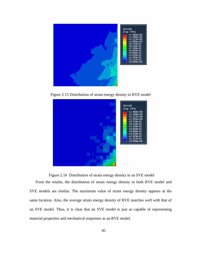
45
Figure 2.15 Distribution of strain energy density in RVE model
Figure 2.16 Distribution of strain energy density in an SVE model
From the results, the distribution of strain energy density in both RVE model and
SVE models are similar. The maximum value of strain energy density appears at the
same location. Also, the average strain energy density of RVE matches well with that of
an SVE model. Thus, it is clear that an SVE model is just as capable of representing
material properties and mechanical responses as an RVE model.

46
Figure 2.17 Comparison between RVE and SVE
Another validation has been implemented to test the effect of SVE on hot spot
locations and in far fields. To ensure that SVE is representative of the bulk material and
mechanical responses, both measures must remain consistent with or without an SVE
implemented in the finite element model. The SVE is expected to have a direct influence
on the local fields near the hot spot due to local crystal plasticity effects. Therefore
implementation of the SVE model at the hot spot will allow calculation of the damage at
the microscale for fatigue life estimation. Figure 2.18 shows comparison of von Mises
stress distributions in the lug joint models, with and without an SVE. The overall
contours show similar trends, i.e., the implemented SVE has a small effect on the
mechanical response outside of the SVE. The hot spot location remains unchanged at the
inside corner radius below the loading pins and the magnitude remains approximately the
same. The distribution of stress in the far field outside of the hot spot position also
remains the same. With the far field value nearly unchanged, the SVE based multiscale
modeling technique is proven capable of representing the homogeneous material outside

47
of the SVE model. Also, the overall mechanical response of the SVE model is almost the
same as the bulk material in the same zone. The introduction of SVE model provides the
possibility to evaluate damage growth based on statistical material properties at the
microscale.
(a)
(b)
Figure 2.18 Local von Mises stress field distribution within lug joint a) with SVE; b)
without SVE.
2.7. Summary

48
Single crystal plasticity was used to capture the crystallographic and geometric
effects of grains at the microscale. The results show that the model can capture local
anisotropic material behavior at grain level. A subroutine UMAT was introduced to
incorporate the single crystal plasticity in the FEA program. Material characterization
was implemented to generate an RVE model at the mesoscale. To improve simulation
efficiency, a SVE model was developed based on the statistical features of material at the
microscale. The SVE captured the statistical distribution of orientation and misorientation
while implementing the average response of geometrical features, including grain
principal axis direction, size, shape, and aspect ratio. A parametric study was performed
to assess the sensitivity of each factor. Principal axis direction and misorientation were
determined to be two of the most important features affecting the mechanical response of
the constructed SVE. The SVE model was verified through comparative simulations to be
capable of representing the bulk material and mechanical responses.

49
3. Physics Based Damage Evaluation & Validation of
Aluminum Alloy 2024-T351
3.1. Introduction
The broad application of metallic materials in many structural components requires a
better understanding of metal fatigue mechanisms. An important first step in metal
fatigue studies is analyzing the initiation of fatigue cracks, which can be decomposed into
two stages: i) nucleation of micro crack and ii) coalescence of micro cracks and
formation of a major crack. Previous work has shown that grain orientation significantly
influences the slip direction and, as a result, also impacts the nucleation mechanics
(Kalnaus, 2006; Groh, 2009; Hochhalter, 2010). Therefore, it can be assumed that fatigue
cracks will nucleate in particular slip directions of polycrystalline material at the
microscale. To capture this phenomenon, an energy and slip-based damage criterion is
developed. It is hypothesized that the micro cracks generated by nucleation grow
individually, coalesce together, and result in a serrated major crack, as shown in Figure
3.1 (a). The serrated shape of the major crack also indicates that the major crack consists
of a set of micro cracks across its path. By studying growth rates and directions of micro
cracks that are governed by slip mechanics and damage accumulations, major crack
formation and propagation can be predicted.
In this chapter, a physics based multiscale damage criterion is developed to simulate
the initiation of fatigue crack growth, including nucleation of micro cracks and formation
of major cracks. The material property and mechanical response of aluminum alloy 2024-

50
T351 are represented using the developed SVE model. The physics of micro crack
nucleation and coalescence is experimentally studied at different length scales and used
as the input for the multiscale model. The micro cracks, which are dominated by shear
crystallographic slipping, nucleate within intermetallic particles. The coalescence of
micro cracks results in the formation of macro crack. The multiscale model and damage
criterion are used to predict fatigue crack growth and direction in polycrystalline
materials. This damage criterion is developed based on single crystal plasticity, and
therefore it only works well in prediction of microstructural small crack growth
(Lankford et al., 1984). As overall fatigue life is most influenced by low growth rate
behavior, the accelerated and subthreshold extension of small flaws can lead to
potentially dangerous over-predictions of life. Relevant lengths of small crack are chosen
to take into consideration the crack categories as defined by Ritchie (1986). In Ritchie‘s
research, it has been shown that crack tip strain fields for large and microstructural small
fatigue cracks, driven by nominally equivalent cyclic stress intensities, are qualitatively
and quantitatively dissimilar. It is thus observed that small cracks and long cracks at the
same nominal driving force can propagate at different growth rates. The microstructural
small crack is defined to be less than 10 times of the critical microstructural dimension,
which is average grain size for polycrystalline materials (Taylor, 2002). In this research,
the average grain area is around 0.0225 mm2 (see Chapter 2). The corresponding grain
size (diameter) is 0.1693 mm based on a hypothesis that the grains are considered in
circular shape. Therefore the microstructural critical small crack length is taken as 1 mm
~ 2 mm for Al 2024-T351. And the size of the corresponding meso SVE is the same as
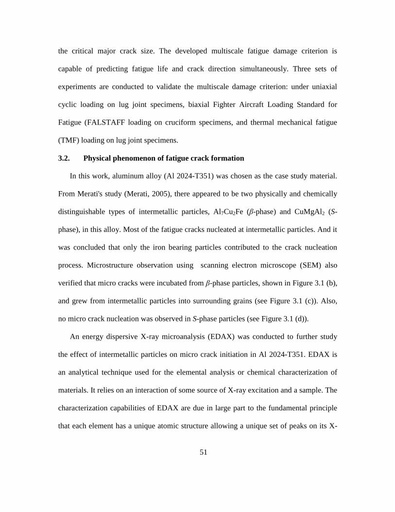
51
the critical major crack size. The developed multiscale fatigue damage criterion is
capable of predicting fatigue life and crack direction simultaneously. Three sets of
experiments are conducted to validate the multiscale damage criterion: under uniaxial
cyclic loading on lug joint specimens, biaxial Fighter Aircraft Loading Standard for
Fatigue (FALSTAFF loading on cruciform specimens, and thermal mechanical fatigue
(TMF) loading on lug joint specimens.
3.2. Physical phenomenon of fatigue crack formation
In this work, aluminum alloy (Al 2024-T351) was chosen as the case study material.
From Merati's study (Merati, 2005), there appeared to be two physically and chemically
distinguishable types of intermetallic particles, Al7Cu2Fe (β-phase) and CuMgAl2 (S-
phase), in this alloy. Most of the fatigue cracks nucleated at intermetallic particles. And it
was concluded that only the iron bearing particles contributed to the crack nucleation
process. Microstructure observation using scanning electron microscope (SEM) also
verified that micro cracks were incubated from β-phase particles, shown in Figure 3.1 (b),
and grew from intermetallic particles into surrounding grains (see Figure 3.1 (c)). Also,
no micro crack nucleation was observed in S-phase particles (see Figure 3.1 (d)).
An energy dispersive X-ray microanalysis (EDAX) was conducted to further study
the effect of intermetallic particles on micro crack initiation in Al 2024-T351. EDAX is
an analytical technique used for the elemental analysis or chemical characterization of
materials. It relies on an interaction of some source of X-ray excitation and a sample. The
characterization capabilities of EDAX are due in large part to the fundamental principle
that each element has a unique atomic structure allowing a unique set of peaks on its X-

52
ray spectrum (Goldstein, 2003). In this study, a damaged sample of Al 2024-T351 was
analyzed using the EDAX technique. A series of intermetallic particles with incubated
micro cracks were observed around major cracks, as shown in Figure 3.2 (a). Some of the
micro cracks nucleated in intermetallic particles and contributed to the generation of a
major crack. Element mappings of Al, Cu, Fe and Mg on the same sample surface are
shown in Figure 3.2 (b), (c), (d), and (e), respectively. The highlighted sites in the
element mapping represent the elements detected by X-ray. The difference between
Al7Cu2Fe (β-phase) and CuMgAl2 (S-phase) intermetallic particles are components Fe
and Mg. Characterization of intermetallic particles, therefore, can be implemented by a
comparison between the element mapping of Fe (Figure 3.2 (d)) and Mg (Figure 3.2 (e)).
The same conclusion was verified in element identification using EDAX, namely, that
micro cracks were incubated from β-phase (iron-rich) particles.
a) b)

53
c) d)
Figure 3.1 SEM observation of major crack and micro crack nucleation: a) major crack
and intermetallic particles in the path; b) micro crack incubation in iron-rich particle; c)
micro crack nucleation in iron-rich particles; d) no micro crack nucleation observed in
magnesium-rich particles.
a) b)
c) d)
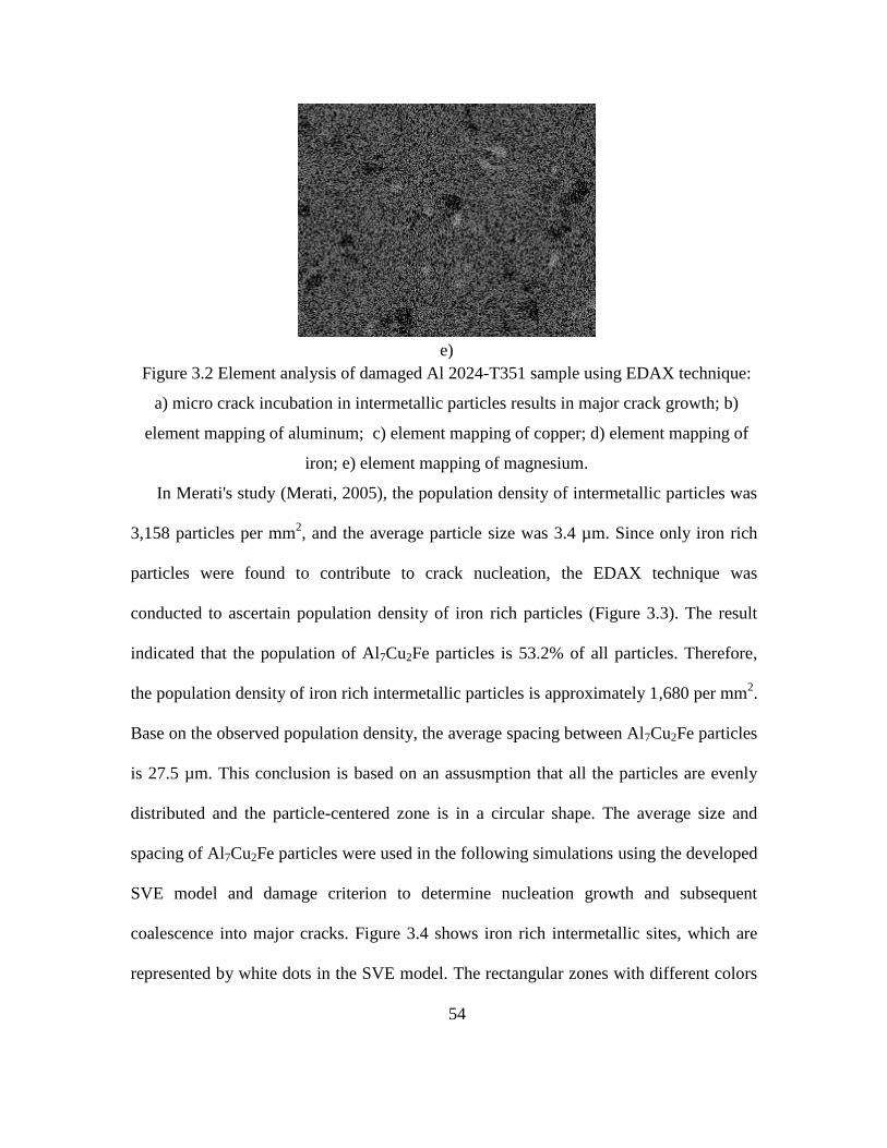
54
e)
Figure 3.2 Element analysis of damaged Al 2024-T351 sample using EDAX technique:
a) micro crack incubation in intermetallic particles results in major crack growth; b)
element mapping of aluminum; c) element mapping of copper; d) element mapping of
iron; e) element mapping of magnesium.
In Merati's study (Merati, 2005), the population density of intermetallic particles was
3,158 particles per mm2, and the average particle size was 3.4 µm. Since only iron rich
particles were found to contribute to crack nucleation, the EDAX technique was
conducted to ascertain population density of iron rich particles (Figure 3.3). The result
indicated that the population of Al7Cu2Fe particles is 53.2% of all particles. Therefore,
the population density of iron rich intermetallic particles is approximately 1,680 per mm2.
Base on the observed population density, the average spacing between Al7Cu2Fe particles
is 27.5 µm. This conclusion is based on an assusmption that all the particles are evenly
distributed and the particle-centered zone is in a circular shape. The average size and
spacing of Al7Cu2Fe particles were used in the following simulations using the developed
SVE model and damage criterion to determine nucleation growth and subsequent
coalescence into major cracks. Figure 3.4 shows iron rich intermetallic sites, which are
represented by white dots in the SVE model. The rectangular zones with different colors

55
represent the grain with variable orientations. The intertmetallic sites represented by
white dots are evenly distributed in the horizontal and vertical direction of SVE model. In
the simulation, the damage index to capture the fatigue damage evolution is calculated
and used to predict crack growth and direction for each intermetallic site. The rectangular
zones with variable colors represent grains with different orientations.
Figure 3.3 EDAX analysis to identify element composition for intermetallic particles.

56
Figure 3.4 Intermetallic points represented in SVE model.
3.3. Damage criterion for nucleation of micro cracks
In order to study multiscale damage effects, it is necessary to take into account crystal
dislocation micromechanics, material microstructure, and macroscale behavior in the
continuum description of finite strain plasticity. Taylor (1938) found that crystal
dislocation provides an atomistic interpretation of the slip mechanics and strain hardening.
His work was followed by many other researchers including Hill (1966) and Asaro
(1977). Their work showed that crystal plasticity is important to incorporate
micromechanical features of plastic flow into macroscopic analysis. In this research,
single crystal plasticity theory is used to describe material behavior in an SVE model
based on the several advantages that it has over other techniques.
In this work, micro crack nucleation is governed by a developed damage criterion,
which is modified from Jiang‘s model (Jiang, 2000). The original damage criterion is as
follows:
(3.1)
where,
. (3.2)
In Equation (3.1) and (3.2), represents the plastic strain energy increment and dD
represents the damage parameter increment in a material plane. represents the normal
stress, and represents the shear stress on a material plane. The quantities and
represent plastic strains corresponding to and respectively. The symbols β and m
0
1 (1 ) ,mmr n
f
dD dY
1,
2
p p
n sdY d d

57
are material constants (see Table 3.1). The symbol < > is the MacCauley bracket (i.e.,
⟨ ⟩ | | ). The quantity is a material memory parameter, and is the
endurance limit of the material and can in essence be considered to be the ‗no-damage‘
level of the fatigue parameter. represents the true fracture stress. More details of this
damage model can be found in Jiang's work (Jiang, 2000).
Table 3.1 Material parameters for Al 2024-T351 (Luo, 2009; Needs, 1987)
m
1.5 0.32 220 MPa 950 MPa 2.323 J/m2
Face centered cubic (FCC) crystal structures, such as Al 2024-T351, are of interest in
this work; therefore, four slip planes {1 1 1} are considered. At the intermetallic particles,
where micro cracks tend to nucleate, the four slip planes are representative of probable
crack planes. At each intermetallic particle, the crack growth direction can be affected by
slip in any combination of the four slip planes, including all. In Jiang‘s criterion (Jiang,
2000), the incremental fatigue damage is dependent on the orientation of the material
plane. However, since the micro crack can initiate and grow in any of the four slip planes,
the critical plane is defined as the material plane where the fatigue damage accumulation
first reaches a critical value. In this research, the damage increment will be applied to
each of the four material planes for each nucleation point, instead of only one single
plane considered in Jiang‘s original study. For FCC structures, the angle between any two
slip planes is always 70.53° (see Figure 3.5 (a)). In order to accommodate multiple slip
planes, the original fatigue damage criteria and plastic strain energy, equations (3.1) and
(3.2), are reformulated to include the dependence on multiple slip planes, equations (3.3)
0 f

58
and (3.4). The degree in which the material planes are dependent is taken into account by
incorporating a dependent factor, δ, in Equation (3.4). For example, for two mutually
perpendicular material planes, the fatigue damages, described in Equation (3.1), are
totally independent. However, if the two material planes have the same orientation, they
are dependent and contribute equally to the plastic strain energy (see Figure 3.5 (b)). In
this case the slip planes are not independent and the dependent factor is used to quantify
the degree of dependence. For two perpendicular planes, of which the cosine value of
their interior angle is zero, the dependent factor is defined as one, since the fatigue
damages in the two planes are totally independent (see Figure 3.5 (c)). For two planes
with the same orientation, of which the cosine value of their interior angle is one, the
dependent factor is defined as two, because the fatigue damages are dependent. For this
research, the cosine value of the angle between any two slip planes (70.53°) is 1/3, and
the total dependent factor for the four material directions is determined to be 4/3 based on
a linear fit. The modified fatigue damage criterion, which has been developed to
accommodate the polycrystalline plasticity theory, can be described as:
(3.3)
(3.4)
where,
represents the damage increment in the αth
slip plane of the ith
intermetallic
particle, the dependent factor can be calculated using Equation (3.5):
(3.5)
( )( ) ( )
0
1 (1 )mmr ni i
f
dD dY
( ) ( ) ( ) ( ) ( )1 1[ ( ) ( ) ]
2
p p
i n sdY d d
( )
idD

59
The ―1‖ and ―2‖ on the right hand side of Equation (3.5) represent the dependent factor
for 90o and 0, respectively; represents the angle between two slip planes, which is
70.53°. Using this linear fit calculation described by Equation (3.5), the dependent factor
for FCC structure is 4/3 (when =70.53°).
a) b)
c) d)
Figure 3.5 a) slip planes in FCC unit cell; b) two perpendicular material planes which are
totally independent; c) two parallel material planes which are totally dependent; d) two
material planes with an arbitrary degree which are partly dependent.
In Luo‘s work (Luo, 2010), an assumption is made that the cumulative damage due to
plastic deformation in the meso RVE should be greater than the minimum energy for

60
creating two free surfaces of a crack. This assumption was used to estimate the crack
growth using the accumulated damage. For aluminum, the surface energy density that
corresponds to the energy variation per unit area due to the creation of surface at room
temperature is 2.323 J/m2
(Needs, 1987). In order to initiate a crack, the minimum energy
required should be 2× ×L, where 2 indicates that there are two free surfaces for one
crack, and L is the crack length. So there is a link between the fatigue damage D and the
crack length L:
. (3.6)
So the modified incremental micro crack length for intermetallic particles could be
described as:
( )
( )
2
i ii
dD AdL
(3.7)
In Equation (3.7), symbol A represents the plastic zone size around the nucleation points.
Using the von Mises yield criterion (Guerra-Rosa, 1984), the plastic zone in plane stress
state as a function of ω is described in Equation (3.8) as,
22
2
3(1 sin cos )
4 2
Ip
ys
Kr
(3.8)
The corresponding plastic zone size can be derived using integral calculus and can be
expressed as:
(3.9)
Since the stress states in nucleation points vary, the plastic zone size is different for
different nucleation points. Finite element simulation has been used to determine the
2DA L

61
plastic zone size. A 2-D finite element model with 29,230 CPS4 elements is generated. In
this model, a small crack with the initial length, 1 μm, is embedded at the center of an
square Aluminum plate. The material property is assumed as isotropic and homogeneous.
Part of the model is shown in Figure 3.6. Static tensile load is applied on the edges of the
plate and perpendicular to the crack surface. This model is used to calculate the plastic
zone size for different stress states. The results show that the plastic zone size in finite
element method simulation (see Figure 3.6) matches very well with the theoretical value,
which is given in Equation (3.9).
Figure 3.6 Plastic zone around the micro crack.
Critical reserved shear stress (CRSS) is an important material parameter, and is
applied as a critical criterion in governing slip (Stoller, 2000). CRSS is the component of
shear stress, resolved in the direction of slip, necessary to initiate slip in a grain. It is a
constant for a given crystal. The ease of slip on different crystal systems is usually
quantified by the CRSS, which is measured in stage I deformation on unconstrained
single-crystal specimens where a unique slip system is activated. Therefore Equation

62
(3.7), which is used to describe the relation between the incremental micro crack length
and the incremental damage index, is available only when the shear stress in the slip
direction is greater than the CRSS value.
Figure 3.7 shows the result of one simulation. In this simulation case, a finite element
model of the lug joint specimen is constructed. A SVE model is embedded at a structural
hot spot to capture the damage. Finite element meshes are used to model the remaining
parts of the component. The lug joint specimen is force controlled cyclically loaded using
a sinusoidal waveform with a load range between 489 N and 4890 N (load ratio 0.1) at a
rate of 20 Hz. The incremental growth of the micro crack length as a function of time for
the three nucleation points (N1, N2, and N3) in each of the four slip planes (slip1, slip2,
slip3 and slip4) are calculated. In this case, micro cracks increase in length only in slip
plane 1 for nucleation point N1 (the black line) and slip plane 3 for nucleation point N3
(the brown line). In the other 10 slip planes of the three nucleation points, the micro crack
does not increase in length because the shear stress in the slip plane fails to reach the
CRSS value so there is no damage increment. Furthermore, in the nucleation directions
mentioned above, the micro crack length increases steadily, cycle by cycle. This
conclusion provides a basis to use a linear fit to extrapolate the micro crack length
increment versus time. Finally, the growth of a micro crack will stop when it reaches a
critical value, 27.5 µm, which is the average length of spacing between neighboring
intermetallic particles. The corresponding physical phenomenon is that the intermetallic
particles have effects in both nucleation and obstruction of micro crack growth. In other

63
words, the micro crack starts from one intermetallic particle and ends in another
intermetallic particle.
a) b)
Figure 3.7 Micro crack length increase cycle by cycle in slip directions.
3.4. Damage criterion for coalescence of micro cracks
In order to model coalescence of micro cracks and the formation of major crack, a
hypothesis is presented in this section. First, the micro cracks in the nucleation points are
projected in an arbitrary direction. Then, the major crack orientation is assumed to be in
the direction in which the sum of length projections of the micro cracks increases at the
highest rate. As shown in Figure 3.8, the micro cracks AB, BC, CD, etc. are projected in
the direction of the arrow line. The corresponding length projections are , , ,
etc., respectively. The major crack length is therefore the sum of the
projections, , , , etc. in the prescribed arrow line direction . Therefore,
the major crack is calculated in Equation (3.10):

64
(3.10)
where, is the direction of the ith
slip plane in th nucleation point, corresponding to
the micro crack length
. θ is the prescribed direction for micro crack projection,
which is assumed to be the probable major crack direction. The range of θ is from –π/2 to
π/2 because the crack grows on two opposite sides of the nucleation point and combines
in the middle to form a single crack. Therefore, the crack is represented by a line,
described by only an angle, as opposed to a vector. By solving for the maximum value of,
Ltotal which is a function of θ, the major crack direction θ and the corresponding major
crack length Ltotal could be calculated.
Figure 3.8 Schematic procedure of projection of micro cracks to major crack.
3.5. Damage criterion for crack formation in thermal mechanical fatigue
Crack initiation and propagation due to TMF loading is one of the major causes of
failure and leads to damage and degradation in aerospace components. TMF loading is
the overlay of a cyclical mechanical loading, which leads to fatigue of a material, with a
cyclical thermal loading. Fatigue damage is primarily due to cyclic creep caused by
vibration loading and temperature cycling. In this research, plastic deformation refers to
4( ) ( )
1 1
( )n
total i i
i
L L cos
( )
i

65
that occurring over almost an instantaneous time scale due to dislocation slip; creep
deformations refer to those occurring over longer time scales due to diffusion-assisted
mechanisms such as grain boundary sliding, dislocation glide/climb, and mass transport
through the grain boundary. Furthermore, there are interactions between vibration and
temperature damage accumulation rates due to temperature dependent changes in
material properties.
A varying temperature condition was generated to simulate a TMF loading case. The
temperature range of thermal cycling is between 100 oC and 200
oC. One thermal fatigue
cycle takes 60 minutes. It takes 20 minutes to increase the temperature from 100 oC to
200 oC at a linear heating rate. Then the temperature is held at 200
oC for 10 minutes and
then decreased to 100 oC in 20 minutes in a linear cooling rate. The value of the linear
heating rate in the temperature increasing stage is equal to the linear cooling rate in the
temperature decreasing stage. Finally, the temperature is held at 100 oC for 10 minutes,
after which the next thermal cycle starts. The variation of temperature in one complete
thermal cycle is shown in Figure 3.9. Compared with thermal cycling, the frequency of
mechanical fatigue is much higher, which is 20 Hz (see Figure 3.10). The time for one
thermal cycle is 72,000 times of that for one mechanical cycle. Therefore, in the
temperature increasing/decreasing stages, the change in temperature is only 0.083 oC
through one mechanical cycle, which is 0.05 second. There is little effect on the
mechanical response and damage evolution of the material from the temperature
difference in one mechanical cycle. So the temperature is assumed to remain constant

66
during one fatigue cycle. The temperature is selected to be the averaged value in the
simulation.
Figure 3.9 Variable temperature condition for thermal mechanical fatigue tests.
Figure 3.10 Variable mechanical load condition for thermal mechanical fatigue tests.

67
The thermal effects on damage evolution include mechanical responses (thermal
creep, elastic modulus and yield strength etc.) and material properties (thermal expansion
factor, density etc.). Generally speaking, temperature will change the dislocation motion,
which plays a critical role in determining the inelastic behavior of a metal and its flow
stress under different load conditions. To deform a metal beyond the elastic limit means
to activate and move its dislocations through the crystal. The approach in this section will
lead to an improved understanding of the fatigue damage characteristics under varying
temperatures. The damage criterion will be taking into account thermal effect and will be
modified to capture crack growth in a TMF load.
In the subroutine UMAT introduced in chapter 2, a power law is used to describe the
strain rate in the flow rule to calculate the slip increment in polycrystal elastoplasticity, as
shown in equations (2.15), (2.16) and (2.17). The relation between shear strain rate and
shear stress (Harper, 1957) can also be described in the form of the power law in
Equation (3.11):
(3.11)
To apply the SVE model and damage criteria to thermal fatigue issues, the Harpor
Dorn creep model is used, where the grain boundary sliding effect and diffusional flow
theory are considered (Harpor, 1957; Kloc, 1977; Ruano, 1988; Wang, 1996; Langdon,
2002). The relation between the applied stress and the steady-state creep rate for Harper–
Dorn creep is phenomenologically described by:
68
(3.12)
where D is the diffusion coefficient for lattice self-diffusion, G is the shear modulus, b is
the Burgers vector, k is Boltzmann‘s constant, T is the absolute temperature, is the
applied shear stress, and A is a dimensionless constant of the order of 10-11
. The
parameters for this material can be found in Table 3.2. In Equation (3.12), the diffusion
parameter D is dependent on temperature and can be expressed as:
(3.13)
Then taking into account temperature effect on creep, a temperature dependent term,
exp( )Q
R T
, is added in Equation (3.12), where Q is the activation energy and R is the
gas constant. As is material constant, which can be calculated by comparing Equation
(3.12) and Equation (3.13) at room temperature (Wilshire, 2008; Warren, 2006; Syed,
2004; Clech, 2004).
(3.14)
Other material properties, such as Young‘s modulus, yield strength, and CRSS are
also dependent on temperature and should be modified in the TMF model. The
temperature dependent Young‘s modulus of Al 2024-T351 can be found in Gibson‘s
work (Gibson, 1997). An increase in temperature expands the crystal lattice, reduces the
stiffness of the bonds, and therefore, causes a drop in the modulus. The temperature
dependence is well approximated in a linear fit:
0 (1 )m
m
TE E
T (3.15)
( ) exp( )n
s
QA
G R T

69
where E0 is the value of the modulus at absolute zero temperature, Tm is the melting
temperature and is a constant, of which the value is close to 0.5, meaning that the
modulus drops by a factor of about 2 in the temperature interval between absolute zero
and the melting point.
m

70
Table 3.2 Creep dependent parameters for Al 2024 (Kassner, 2007; KLOC, 1997; Yavari,
1982)
Parameter Value
A: Dimensionless constant 3.5E-11
D: Diffusion coefficient 1.86E-4
R: Gas constant 8.314 Jmol-1
K-1
Q: Activation energy 143.4 kJ/mol
G: Shear modulus 3.022E4-16×T MPa
b: Burgers vector 2.86E-10 m
k: Boltzmann constant 1.381 × 10⁻²³
JK-1
n: Stress exponent 3
The yield strength decreases with increasing temperature for Al 2024 T 351 (Gibson,
1997). On a microscopic scale, thermal energy activates dislocations and causes them to
move a little more easily; this imparts a temperature dependence to the yield strength.
Kinetic models (Kocks, 1975) lead to equations for yield by thermal plasticity, which
simplify to a form:
(3.16)
where is the yield strength at absolute zero temperature, A is a constant of general
order of 0.04, and 0s is a kinetic constant of about 106 /s. The equation summarizes the
experimental observations, namely, at near room temperature, the yield strength
0 0
0(1 ln )s s
ys ys
s m
G A T
G T
0
ys

71
decreases linearly with increasing temperature, and logarithmically with decreasing strain
rate.
When a single crystal specimen is loaded, the applied stress is resolved on the slip
planes in the material at grain level. The resolved shear stress, τs on any given plane is
determined by the angle between the plane normal and the applied stress direction.
Yielding occurs as a result of dislocation slip when the resolved shear stress on one of the
planes exceeds a critical value. The relationship between applied stress and resolved
shear stress is the same in a polycrystalline material, but is complicated by the fact
thatmaximum resolved shear stress will vary from one grain to another. In addition,
material compatibility and continuity act to limit the deformation of any one grain that
may be favorably oriented for slip. By applying a simple compatibility criterion and
assuming that all the grains in the material deformed uniformly, Taylor (1938) derived a
relationship between yield strength and the resolved shear stress in polycrystalline
material. Such an analysis amounts to determining an effective average reciprocal
Schmid factor for the polycrystalline material. The average value obtained by Taylor for
FCC aluminum was about 3.06 and has since been termed the Taylor factor (Stoller,
2000). Therefore, the temperature dependent CRSS can be calculated by temperature
dependent yield strength:
(3.17) 1
ysCRSSm

72
where m is the Taylor factor, with a value of 3.06. For aluminum alloys, the yield
strength, which is a temperature dependent material property, decreases with increasing
temperature (Lipski, 2012).
The thermal expansion factor of Al 2024-T351 increases with increasing temperature,
a phenomenon studied by Fridman (Fridman, 1975), and as shown in Table 3.3. In the
temperature range between 100 oC and 200
oC, the change of the thermal expansion
factor is around 2×10⁻⁶
/oC. Also, in this approach, the mechanical load is force control
instead of displacement control. So the thermal expansion has little effect on stress
distribution and damage evaluation, and is ignored in the TMF model.
Table 3.3 Thermal expansion factor of Al 2024-T351 (Fridman, 1975).
Temperature (°C) 20 77 127 227 327 427
Thermal Expansion
(10-6
/°C) 23.0 24.1 24.9 26.5 28.2 30.4
Based on the thermal effects discussed above, the damage criterion will be modified
to capture damage accumulation under variable temperature. All the temperature
dependent factors (Young‘s modulus, yield strength and CRSS) were updated in the
subroutine UMAT. In this simulation, a finite element model of the lug joint specimen is
constructed. A SVE model is embedded at a structural hot spot to capture the damage.
Finite element meshes are used to model the remaining parts of the component.
Comparison between different working temperatures is constructed to study the thermal
effect on damage evolution. The material for the specimen is Al 2024-T351. The lug joint
specimen is cyclically loaded using a sinusoidal waveform with a load range between 489
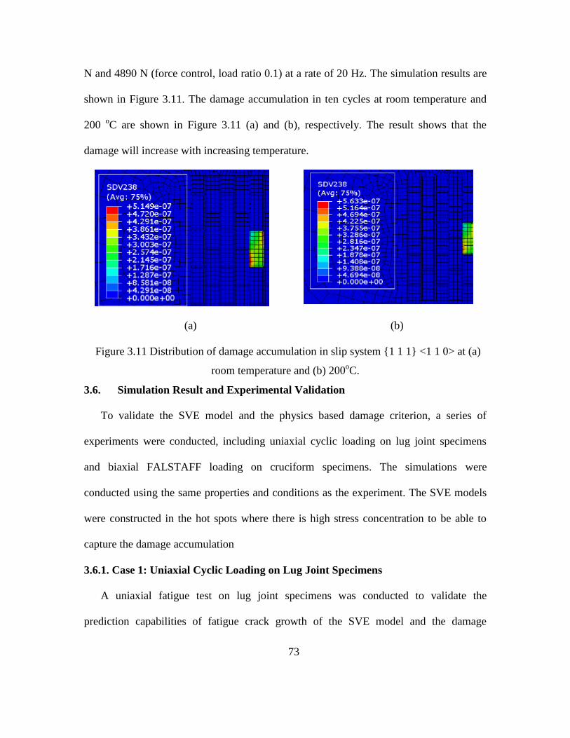
73
N and 4890 N (force control, load ratio 0.1) at a rate of 20 Hz. The simulation results are
shown in Figure 3.11. The damage accumulation in ten cycles at room temperature and
200 oC are shown in Figure 3.11 (a) and (b), respectively. The result shows that the
damage will increase with increasing temperature.
(a) (b)
Figure 3.11 Distribution of damage accumulation in slip system {1 1 1} <1 1 0> at (a)
room temperature and (b) 200oC.
3.6. Simulation Result and Experimental Validation
To validate the SVE model and the physics based damage criterion, a series of
experiments were conducted, including uniaxial cyclic loading on lug joint specimens
and biaxial FALSTAFF loading on cruciform specimens. The simulations were
conducted using the same properties and conditions as the experiment. The SVE models
were constructed in the hot spots where there is high stress concentration to be able to
capture the damage accumulation
3.6.1. Case 1: Uniaxial Cyclic Loading on Lug Joint Specimens
A uniaxial fatigue test on lug joint specimens was conducted to validate the
prediction capabilities of fatigue crack growth of the SVE model and the damage

74
criterion. Lug joint specimens were machined from a bulk Al 2024-T351 plate with the
rolling direction lengthwise along the lug joint (see Figure 3.12b). The specimens were
cyclically loaded in a servo hydraulic desktop test frame using a sinusoidal waveform
with a load range between 489 N and 4890 N (load ratio 0.1) at a rate of 20 Hz. MTS
Bionix 370.02 test frame (with the maximum loading capability 22.2 kN) was used to
conduct the fatigue test (Figure 3.13). To validate the multiscale model, the number of
cycles necessary to achieve a 1 mm crack was obtained experimentally and a total of five
specimens were tested. The experimental results are summarized in Table 3.4. A final
image at failure of one specimen illustrating the crack angle is shown in Figure 3.12 (a).
The mean deviation for the number of cycles to produce a 1 mm crack was in the range
from 68 K to 98 K cycles. Among the five tests, there are two tendentious crack
directions: around -4º (specimens 1 and 2) and -28º (specimens 3, 4 and 5). The reasons
that there is no single probable crack direction include the effect of the microstructural
polycrystalline, geometry of specimen, loading condition, and stress distribution in the
hot spot.

75
(a)
(b)
Figure 3.12 Lug joint specimen for fatigue test: a) crack initiates in the shoulder of lug
joint and b) geometric dimension.
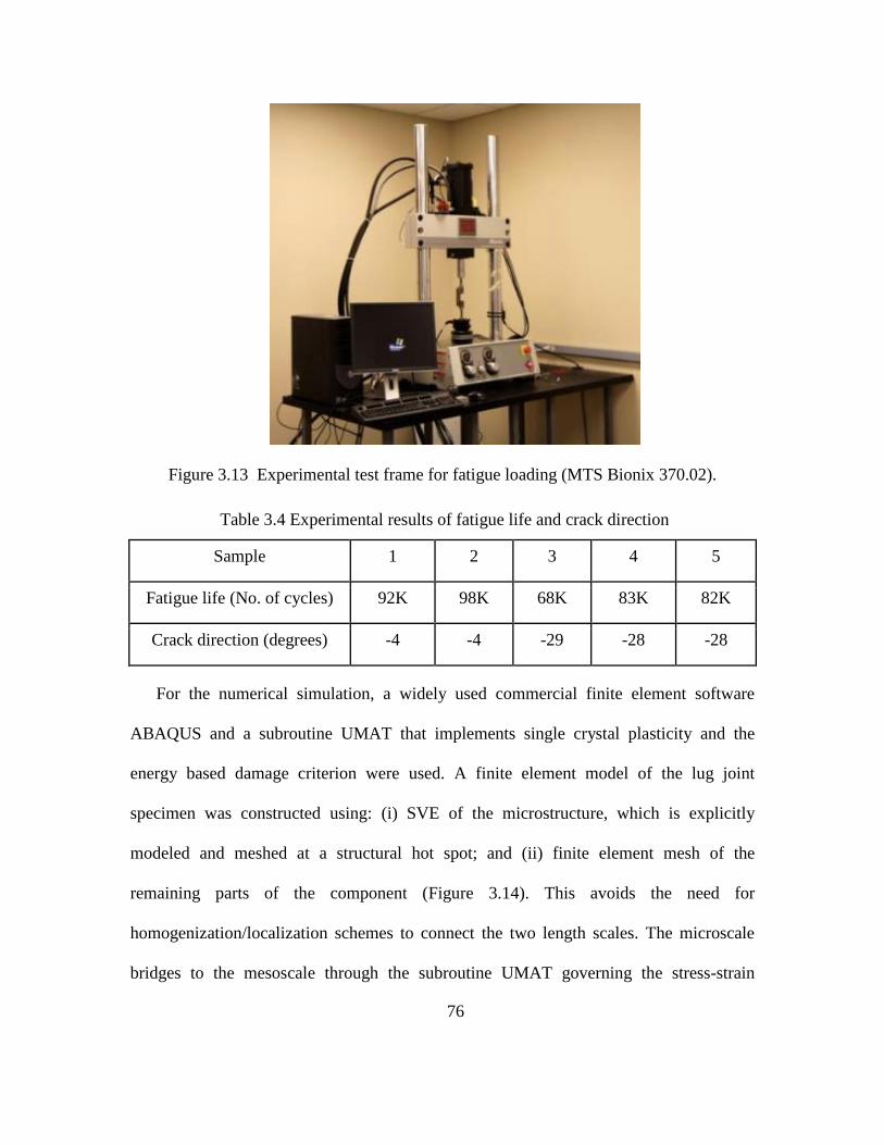
76
Figure 3.13 Experimental test frame for fatigue loading (MTS Bionix 370.02).
Table 3.4 Experimental results of fatigue life and crack direction
Sample 1 2 3 4 5
Fatigue life (No. of cycles) 92K 98K 68K 83K 82K
Crack direction (degrees) -4 -4 -29 -28 -28
For the numerical simulation, a widely used commercial finite element software
ABAQUS and a subroutine UMAT that implements single crystal plasticity and the
energy based damage criterion were used. A finite element model of the lug joint
specimen was constructed using: (i) SVE of the microstructure, which is explicitly
modeled and meshed at a structural hot spot; and (ii) finite element mesh of the
remaining parts of the component (Figure 3.14). This avoids the need for
homogenization/localization schemes to connect the two length scales. The microscale
bridges to the mesoscale through the subroutine UMAT governing the stress-strain

77
response of an element within the SVE. This multiscale model is applied to solve the
problem of efficiently predicting crack initiation and direction within the component.
Three simulation test cases were constructed with different SVE models based on the
statistical orientation pool. Figure 3.15 shows the most probable major crack direction
and corresponding increment of crack length per loading cycle. Results of fatigue cycles
prediction to reach 1 mm crack length and probable crack directions are shown in Table
3.5.
Figure 3.14 Boundary conditions and implementation of a two-scale mesh at the
structural hot spot of an aluminum lug joint.
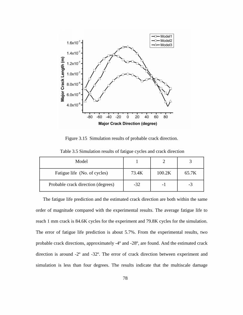
78
Figure 3.15 Simulation results of probable crack direction.
Table 3.5 Simulation results of fatigue cycles and crack direction
Model 1 2 3
Fatigue life (No. of cycles) 73.4K 100.2K 65.7K
Probable crack direction (degrees) -32 -1 -3
The fatigue life prediction and the estimated crack direction are both within the same
order of magnitude compared with the experimental results. The average fatigue life to
reach 1 mm crack is 84.6K cycles for the experiment and 79.8K cycles for the simulation.
The error of fatigue life prediction is about 5.7%. From the experimental results, two
probable crack directions, approximately -4º and -28º, are found. And the estimated crack
direction is around -2º and -32º. The error of crack direction between experiment and
simulation is less than four degrees. The results indicate that the multiscale damage

79
model can successfully capture the fatigue crack growth and direction and is expected to
provide good estimates of fatigue life of Al 2024-T351.
The error in fatigue life prediction can be attributed to several possible factors. First,
one possible reason is that the magnitude of the surface energy density (in Equation 3.7)
of a bulk homogenized material is most likely not the same as that within a grain. As a
result, a difference between local information in grains and average global information in
SVE is expected. Second, the micro crack nucleates and grows first in grains, of which
the growth rate of damage accumulation in the slip directions is relatively higher.
Loading conditions vary across different positions of the structural component. The same
grain orientation under different loading conditions shows significantly different
sensitivities. The stochasticity in grain orientation distribution in both actual specimens
and SVE models is another reason for the difference. Finally, in the simulation, the
material property corresponds to an ideal and healthy state. There are no flaws and voids
in the modeling before loading. Also the intermetallic particles are constructed with the
same size, and arranged in the SVE model with the same spacing distance. So the
presence of defects, flaws, and large intermetallic particles in the real material will affect
the fatigue life.
3.6.2. Case 2: Biaxial FALSTAFF Loading on Cruciform Specimens
FALSTAFF loading typically occurs at the wing root area of a fighter-type aircraft.
For this reason, it has been widely used in numerous fatigue research programs (Schijve,
2004). A modified block of FALSTAFF loading, including 79 cycles, is used as shown in
Figure 3.16. To approach the fatigue crack initiation and growth under biaxial

80
FALSTAFF loading, the root mean square method (RMS) is introduced to simplify the
complex loading history. In previous studies, the RMS model was shown to be a simple,
reliable, and efficient method to approach random loading (Kim 2006).
Figure 3.16 FALSTAFF loading (79 cycles)
In previous study by Mohanty (2010), cruciform specimens were subjected to biaxial
fatigue loading. The cruciform specimens were machined from a bulk Al 2024-T351
plate with the rolling direction along one symmetrical axis. The specimens were
cyclically loaded under force controlled biaxial FALSTAFF loading with a frequency of
20 Hz. The loading is shown in Figure 3.16. An example of the cruciform specimen is
shown in Figure 3.17. The area of the center span is 62.66 mm by 62.66 mm, and the
thickness is 2.54 mm. The diameter of the center hole is 6.35 mm. A 1 mm width notch
was introduced at the center hole along a 45° angle with respect to the vertical direction.
Since there is high stress concentration at the tip of the notch, the probability of crack

81
initiation is greatly increased, therefore creating a structural hot spot. Following this
observation, the SVE model is embedded in the hot spot location of the cruciform. The
length of the notch is 1.5 mm. Therefore the SVE size is designed to be 3 mm × 3 mm to
cover the whole length of the notch. The notch tip is almost at the center of the SVE
model.
a) b)
c) d)

82
Figure 3.17 Cruciform specimen: a) a round hole in center for test; b) a 45° notch at the
center hole for fatigue test; c) geometric dimension of cruciform; d) geometric dimension
of the center.
Before conducting the fatigue life prediction simulation, validation of mechanical and
damage responses were performed to ensure the RMS model could be used to accurately
represent the FALSTAFF loading. The RMS method, which is also known as the
quadratic mean method, is a statistical measure of the magnitude of a varying quantity. It
can be calculated for a series of discrete values. In this approach, there are 79 sinusoids
cycles in one block of FALSTAFF loading (see Figure 3.16). So there are 79 maximum
and 79 minimum loading values, which can be used to represent the variability of the
loading. The RMS model is used to simplify the complex loading history. The RMS
values for the 79 maximum loading values and the 79 minimum loading values are
calculated respectively. The tests were assumed to be under constant amplitude loading.
The following relationships are used to obtain the RMS loadings:
1/22
max max,
1
1( )
N
rms i
i
Load LoadN
(3.17)
1/22
min min,
1
1( )
N
rms i
i
Load LoadN
(3.18)
Using Equations (3.17) and (3.18), the complex FALSTAFF loading is converted into a
simplified loading condition based on the RMS model, as shown in Figure 3.18.

83
In a previous study on damage criteria, the fatigue damage was determined to be
significantly dependent on the plastic strain energy (Jiang, 2000; Luo, 2011). Therefore,
the accumulation of plastic strain energy density can be used as an important criterion to
validate the RMS model. For comparison, two simulations were conducted with the same
cruciform finite element model, but under two different loading conditions, i.e.,
FALSTAFF and RMS loading.
The distributions of plastic strain energy density after 79 loading cycles is shown in
Figure 3.19. The square blocks represent the SVE area. From this result, the plastic strain
energy shows similar distributions for FALSTAFF and RMS loadings. This indicates that
RMS methods can provide a good representation of local damage accumulation.
Furthermore, the average value of plastic strain energy density is another index to
Figure 3.18 RMS model based loading (79 cycles)

84
measure the total response to damage accumulation. The accumulated average plastic
strain energy density within the SVE model during 79 cycles (one repeating block) for
FALSTAFF and RMS loading are shown in Figure 3.20. The FALSTAFF and RMS
models show a linear increase of plastic strain energy accumulation. After 79 loading
cycles, the average plastic strain energy density is 32.59 MPa for FALSTAFF and 32.87
MPa for the RMS model. The difference between FALSTAFF and the corresponding
RMS model is only 0.85%. Therefore, the RMS model can be used to simply and
accurately represent the complex loading case.
a) b)
Figure 3.19 Distribution of plastic strain energy density in a) RMS model after 79
cycles; b) FALSTAFF model after 79 cycles

85
Figure 3.20 Average plastic strain energy density in SVE model for FALSTAFF & RMS
loading conditions with a frequency of 20Hz.
A series of experiments of biaxial FALSTAFF loading on cruciform specimens were
conducted using an MTS biaxial tension-torsion test system (with the maximum loading
capability 97.9 kN) as shown in Figure 3.21. The cruciform specimens were machined
from a bulk Al 2024-T351 plate with the rolling direction along one symmetrical axis.
The specimens were cyclically loaded under biaxial FALSTAFF loading with a
frequency of 20 Hz. To validate the multiscale model, the number of cycles necessary to
achieve a 3 mm crack was obtained experimentally. A total of four specimens were tested
(see Figure 3.22). The crack generated from the notch tip, which was oriented at 45º from
the loading direction. The experimental results are summarized in Table 3.6 (Mohanty,
2010). The average cycle number to produce a 3 mm crack was 42.0K cycles, and the
mean crack direction was 58.8o.

86
Figure 3.21 MTS biaxial tension-torsion test system
Table 3.6 Experimental results of fatigue life and crack direction (Mohanty, 2010)
Sample 1 2 3 4 Average
Crack direction (degrees) 57 56 56 66 58.8
Average fatigue life
(No. of cycles) 42.0K
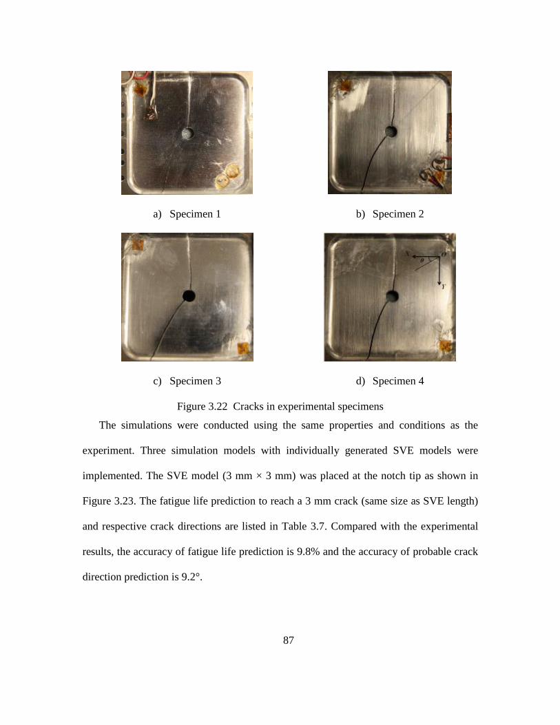
87
a) Specimen 1 b) Specimen 2
c) Specimen 3 d) Specimen 4
Figure 3.22 Cracks in experimental specimens
The simulations were conducted using the same properties and conditions as the
experiment. Three simulation models with individually generated SVE models were
implemented. The SVE model (3 mm × 3 mm) was placed at the notch tip as shown in
Figure 3.23. The fatigue life prediction to reach a 3 mm crack (same size as SVE length)
and respective crack directions are listed in Table 3.7. Compared with the experimental
results, the accuracy of fatigue life prediction is 9.8% and the accuracy of probable crack
direction prediction is 9.2°.

88
Figure 3.23 Loading conditions and implementation of SVE model at the structural
notch tip of an Al 2024-T351 cruciform.
Table 3.7 Fatigue cycles prediction to reach a 3 mm crack and corresponding direction
Model 1 2 3 Average
Probable crack direction (degrees) 76 75 52 68
Fatigue life (No. of cycles) 25.0K 47.0K 66.3K 46.1K
There are also several additional possible factors for errors in biaxial FALSTAFF
experiments. First, the RMS model is introduced in the analysis to simplify the loading
condition. Although the validation of the RMS model shows the difference from
FALSTAFF loading condition as being only 0.85%, loading history can also affect the
fatigue life and crack direction, especially in the context of the high loading points in the
FALSTAFF model. Also, the pre-implemented notch in the middle circle can be
considered to be an existing major crack, which leads to higher stress and damage
concentration in the hot spot. In addition to the nucleation and coalescence of micro

89
cracks inside materials, there is also the macro crack propagation effect at the notch in the
hot spot. So, the final crack can also be attributed to the major crack propagation effect.
This observation can also explain why the accuracy in case 2 is lower than in case 1.
3.6.3. Case 3: TMF Loading on Lug Joint Specimens
In the TMF test, a lug joint specimen having the same dimension and material as in
case 1 was used. The experiments here were conducted under simultaneous mechanical
loading and thermal cycling (see Figure 3.9 and Figure 3.10). The specimens were
cyclically loaded using a sinusoidal waveform with a load range between 489 N and 4890
N (load ratio 0.1) at a rate of 20 Hz. It takes one hour for one temperature cycle, and the
fatigue frequency is much higher than thermal frequency. So the temperature is
considered to be constant in each fatigue cycle. To validate the multiscale model, the
number of cycles necessary to achieve a 1 mm crack was obtained experimentally.
In order to get material properties including Young‘s modulus and a yield strength of
Al 2024-T351 from the experiments, a series of tensile tests under different temperatures
were conducted. The dog bone specimen was designed and used in the thermal tensile
test. The dimension of the dog bone specimen is shown in Figure 3.24(a). The
temperatures in the tensile tests are room temperature, 100 oC, 150
oC, 200
oC and 250
oC. All the final cracks take place in the middle of the specimens (see Figure 3.24(b)).
The thermal tensile test was conducted using the Instron material test frame 985 with a
thermal chamber (see Figure 3.25).

90
a)
b)
Figure 3.24 Dog bone specimen for tensile test at different temperatures: a)
geometric dimension and b) crack takes place in the middle of dog bone specimen.

91
Figure 3.25 Instron material test frame 985 with thermal chamber.
The stress-strain curves of the tensile tests as shown in Figure 3.26, show that the
yield strength decreases with increasing temperature. The CRSS can be calculated based
on yield strength using Equation 3.16. The CRSS decreases with increasing temperature
as well. The Young‘s modulus decreases slightly with increasing temperature. In the
TMF test, the temperature range is between 100 oC and 200
oC. The related material
properties in this temperature range are listed in Table 3.8. The material properties in
other temperatures are calculated using the linear interpolation method.

92
Figure 3.26 Stress-strain relation of Al 2024-T351 at different temperatures
Table 3.8 Young‘s modulus, yield strength, and CRSS of Al 2024-T351 at different
temperatures
Temperature (oC) Young‘s modulus (GPa) Yield strength (MPa) CRSS(MPa)
100 71 375 168
150 68 350 157
200 63 320 146
Taking into account the variable temperature conditions in the TMF test (see Figure
3.9), three damage models are used to solve this thermal mechanical fatigue case: I)
cycled loading in 100oC, II) cycled loading in 200
oC and III) cycled loading in the
temperature varying between 100oC and 200
oC. For the two constant temperature
conditions, the damage increment and crack growth rate governing the function in
Equations (3.3) and (3.6) can be used directly based on temperature dependent material
properties (i.e., Young‘s modulus, yield strength, CRSS, and creep parameters). The crack
coalescence criterion described in Equation (3.9) can be used directly as well. For the

93
variation temperature stages (between 100 oC and 200
oC), a set of temperature dependent
models were applied under different temperatures, respectively. The weight averaged
method was used to get the comprehensive effect in one thermal cycle, as shown in
Equation (3.19):
L =
(3.19)
where L is the comprehensive crack growth rate, L1, L2 and L3 are crack growth rates at
stage 1 (100oC), stage 2 (100
oC - 200
oC), and stage 3 (200
oC), respectively. t1, t2 and t3
are weight factors, which are equal to the time length of stage 1, stage 2, and stage 3,
respectively.
The crack growth rates in different stages are listed in Table 3.9. It shows that the
crack grows faster at higher temperatures. The time lengths of the three different stages
are used as weight factors to calculate the average crack growth rate in one block (one
hour). The simulation result shows that the predicted fatigue life is 67.6K cycles to form
a 1mm crack. Thermal mechanical fatigue tests were conducted and the average fatigue
life was seen to be 62.4K cycles. The error between simulation and experiment is 7.7%.
The simulation result shows a good match with the experimental results.
Table 3.9 Fatigue Crack Growth Rate Estimation of TMF Simulation
Temperature (oC) Time in one thermal cycle (min) Crack growth rate (mm/cycle)
100 10 5.03E-10
100 - 200 40 5.92E-10
200 10 6.79E-10

94
Compared with the fatigue test conducted under room temperature, some material
properties needed to be updated in the TMF test, which resulted in temperature dependent
damage accumulation. However, the damage indexes in the 12 slip systems are changed
proportionally and in the same ratio. Therefore, it can be concluded that the temperature
only affects the crack growth rate, but not the crack direction, which is determined by
equation (3.9). For the TMF test, the estimated crack direction is the same as case 1,
which is around -2º and -32º. From the experimental results (see Figure 3.27), two cracks
grow simultaneously at the shoulders of the lug joint specimen. The averaged crack
direction in the experiment is -29o. The error in crack direction between experiment and
simulation is 3 degrees. The results indicate that the thermal fatigue damage model can
capture the thermo-mechanical fatigue crack growth.
Figure 3.27 Crack initiation takes place in shoulders of lug joint specimen in TMF test.
3.7. Summary

95
In this chapter, a physics and slip based multiscale damage criterion is developed to
predict fatigue life and crack direction in aluminum alloy based complex components.
Three different length scales are considered in this study. At the microscale, a damage
criterion based on single crystal plasticity theory is developed to approach micro crack
nucleation, which occurs in iron-rich intermetallic particles and grows into the
surrounding grains. At the mesoscale, a computationally efficient SVE model is
constructed to represent material property and mechanical response in the hot spot. The
fatigue life and corresponding crack direction are predicted by the simulation. At the
macroscale, a finite element analysis of components (lug joint and cruciform specimens)
is conducted with the meso SVE bridging two-scale meshes. Results indicate that the
physics based damage criterion is capable of capturing nucleation and coalescence of
micro cracks in different scales. It also provides the possibility of bridging energy-based
damage in intermetallic particles and crack initiation in structural components. Compared
with a conventional RVE model, the SVE model significantly improves the preprocessing
efficiency as well as computational efficiency through reduced number of meshes. The
temperature dependent creep effect on the slip mechanism is also considered. The power
law that is used to describe the strain rate in the flow rule to calculate the slip increment
in the subroutine UMAT is modified to solve the thermal mechanical fatigue problem.
The simulation results from the developed multiscale damage criterion show good
correlation with the experimental results while ensuring computational efficiency. The
results show that the multiscale damage criterion can successfully capture crack initiation
and predict fatigue life.

96
4. Development of Spring-bead Based Network Model
to Simulate a Self-sensing Polymeric Material Response
4.1. Background
Mechanically sensitive mechanophores are covalently linked into polymers to lead to
specific chemical reactions upon mechanical loading. Mechanophores open a novel way
for designing multifunctional self-sensing materials (Chang, 1987; Thostenson, 2006;
Wu, 2008). To model polymeric systems integrated with nanoparticles, numerous
different approaches have been developed. These include homogenization techniques,
molecular dynamics (MD) simulation, Monte Carlo (MC) simulation and the Mori-
Tanaka approach. The high computational cost associated with large-scale MD
simulations limits its use beyond the nanoscale whereas the use of micromechanical
homogenization techniques in a multiscale framework can lead to the propagation of
large errors across length scales. A major challenge is how to scale material behavior
from the nano-, micro-, and mesoscales to the macroscale in order to investigate the
effect of the self-sensing material at the structural scale. Despite the accuracy of MD
simulations, computational inefficiency prohibits their use within a multiscale analysis
framework. In order to maximize computational efficiency and maintain high accuracy
while investigating the material behavior of polymers, a novel multiscale modeling
framework was developed in this research. The simulation techniques include MD
simulation at the atomistic scale, spring-bead model at the microscale, crosslinked
network model at the mesoscale, and FE simulation at the macroscale.

97
This chapter presents a spring-bead model and a network model which are developed
to bridge nanoscale information to higher length scales for modeling epoxy polymers
embedded with smart particles (see Figure 4.1). Because mechanical properties are
determined by inter/intra-molecular potential energy and there is no reported literature on
the mechanical properties of the self-sensing polymer, MD simulation is the most
appropriate approach to understanding the material properties of the self-sensing polymer
at the microscale. A series of MD simulations are performed to capture the generation of
crosslinked bonds in the self-sensing polymer; this information is further used to
construct the probability distribution of crosslinking degrees. At the mesoscale, the
material is partitioned into discrete mass beads which are linked using linear springs. By
integrating multiple spring-bead models, a crosslinked network model is generated to
represent the elastic material properties at the mesoscale. The spring-bead based network
model is integrated with FE model to characterize the mechanical properties at the
macroscale. The developed methodology is computationally efficient and provides a
possible means to bridge various length scales without significant loss of accuracy.

98
Figure 4.1 Modeling of self-sensing polymer materials at the microscale, mesoscale, and
macroscale.
4.2. MD simulation of bond clusters at the microscale
4.2.1 Self-sensing behavior of the smart material
MD simulation is used to characterize the mechanical properties of this self-sensing
polymer at the molecular level. A stochastic approach is used to estimate the most likely
crosslinking degree of the polymer system. Some relevant research efforts
(Bandyopadhyay, 2011; Li, 2010; Tack, 2008) estimated the crosslinking degree
indirectly by comparing the Tg obtained from MD simulations, and from differential
scanning calorimetry (DSC). In this study a direct approach to estimate the local
crosslinking degree is introduced; this direct method mimics the curing process based on
inter/intra molecular potentials. The inter/intra molecular potentials are determined by a
force field, which is a set of functions and parameters achieved from experimental or
quantum mechanical studies to describe material properties at the molecular level. The
Merck molecular force field (MMFF), which was developed for general organic research
and pharmaceutical development that requires the most accurate results, is used for the
epoxy-based systems used in this study (Yang, 2012; Halgren, 1996). The MD
simulations are performed using the Large-scale Atomic Molecular Massively Parallel
Simulator (LAMMPS) package (Plimpton, 2007).

99
Figure 4.2 Schematic of UV-initiated cyclobutane generation and damage-induced
cinnamoly group generation.
The self-sensing material modeled in this work comprises Tris-
(Cinnamoyloxymethyl)-Ethane (TCE) monomer to synthesize cyclobutane - a
mechanophore formed by exposing the TCE monomer to UV light (wavelengths of range
330-380 nm), as shown in Figure 4.2. With local damage, the physical discontinuities
break the covalent bonds in cyclobutane. Subsequently, the cyclobutane transforms into
the TCE monomer, which consists of cinnamoyl groups that emit visible light of wave-
lengths ranging from 450 nm to 600 nm under UV excitation (Chung, 2004; Cho, 2008,
2010). Figure 4.3 shows the results observed from this self-sensing material surface of a
specimen during a uniaxial loading test. The UV fluorescence images were taken at
different stages of load increment. There is no fluorescence observed in the initial range
of the loading (see Figure 4.3a); fluorescence can be observed when micro cracks initiate
in the specimen (the green scatter points in Figure 4.3b). The intensity of the fluorescence
keeps increasing with the growth of the micro cracks (the green zone in Figure 4.3c). The
mechanophore response is a result of the transmission of external force at the macroscale
to the debonding of covalent links at the molecular level (Kingsbury, 2011; Silberstein,

100
2013). This observation provides evidence that the self-sensing material has the potential
to capture various levels of damage progression. MD simulation is adopted to further
understand the interactions between the epoxy/hardener and the self-sensing material,
which could affect the color changing phenomena significantly. Two important features
of the material are required from the MD simulation to construct the spring-bead model
that can represent various crosslinking degrees at the microscale: statistical distribution of
crosslinking degree and corresponding mechanical properties.
a) b) c)
Figure 4.3 Fluorescence observation in self-sensing polymer with increasing load: a) no
crack and no fluorescence observed; b) micro crack and slight florescence intensity; c)
major crack and higher florescence intensity.
4.2.2 Statistical crosslinking degree in MD simulation
The molecular structures of the epoxy resin and the hardener that form the polymer
used in this study are Di-Glycidyl Ether of Bisphenol F (DGEBF) and Di-Ethylene Tri-
Amine (DETA), respectively (see Figure 4.4a and 4.4b). The smart particle responsive to
mechanical loading is TCE (see Figure 4.4c). A stochastic approach is proposed to
capture the variability of the crosslinking degree and the mechanical properties of the
polymer system; an RVE model is constructed with molecules (of the resin, the hardener,
and the smart particle) distributed randomly in the initial configuration (Figure 4.4d).
The RVE size is 14 nm × 14 nm × 14 nm. The weight percentages of the components in

101
this self-sensing polymer are 70.9% for DEGBF, 19.1% for DETA, and 10.0% for TCE.
Table 4.1 shows the respective chemical formulae, weights, and numbers of component
molecules.
Figure 4.4 Components of self-sensing polymer: a) epoxy resin, b) hardener, c) smart
material to form, and d) RVE model.
Table 4.1 Components in the self-sensing polymer
Formula Weight Molecule number in one RVE
DGEBF C19H20O4 313 g/mol 650
DETA C4H13N3 103 g/mol 550
TCE C32H30O6 510 g/mol 50
The epoxy based polymer is an extensively crosslinked structure; additionally, the
extent of crosslinking significantly affects the mechanical properties. The crosslinking
degree is defined as the percentage of actual crosslinked covalent bonds over all potential
crosslinked bonds. It is important to estimate the crosslinking degree accurately to
capture the mechanical properties at the microscale. The crosslinking degree in the
network structure is defined in Equation (4.1):

102
(4.1)
where is the crosslinking degree, and are the number of the actual and
all potential crosslinked covalent bonds in a certain zone, respectively. A schematic of
the epoxy network structure is shown in Figure 4.covalent bonds (represented are
represented by a black solid line in Figure 4.5c. The blue ellipse R (Figure 4.5a) and the
red circle H (Figure 4.5b) represent the epoxy resin and hardener, respectively. For epoxy
resin particles there are two active sites (yellow points in Figure 4.5a), and for hardener
particles there are five active sites (purple points in Figure 4.5b). A covalent bond can be
generated when the distance between the active sites of the epoxy resin and the hardener
is shorter than a critical value. The two active sites can share their electrons to stabilize
the potential energy. The process of bond formation between the epoxy resin and the
hardener molecules is also known as ―curing‖ in polymer science.
Figure 4.5 Schematic of crosslinked structure of epoxy resin and hardener: a)
molecular structure of epoxy resin with two active sites; b) hardener with five active
sites; c) epoxy resin and hardener are crosslinked to generate polymer structure. Black

103
solid lines represent covalent bonds.
Figure 4.6 Statistical distribution of crossing-linking degrees based on MD simulations
(N = 500).
A total of 500 MD simulations were performed, each with a randomly generated
initial configuration (42,350 atoms in each RVE) at standard room conditions (300K and
1atm). The RVE size is 14 nm × 14 nm × 14 nm. The 500 repeating MD models ensure
that the simulation results can characterize the statistical distribution of material
properties. In the simulation, each RVE was cured using a bond formation command in
LAMMPS and a crosslinking cut-off radius of 4.0 Angstroms; this cut-off radius was
selected because it is more than twice the length of a carbon-nitrogen covalent bond
(Varshney, 2008; Yu, 2009). The resulting crosslinking degree is unique for each RVE
due to the random initial configuration. The frequency distribution of resulting
crosslinking degrees (Figure 4.6) from the 500 MD simulations is statistically smooth.
The simulation results indicate a quasi-normal distribution with crosslinking degrees

104
ranging between 40% and 65%. The average crosslinking degree is 52.72% for the
polymer system containing the self-sensing material. These results are used to construct
the statistical network model at the mesoscale.
4.2.3 Mechanical properties of self-sensing polymer in MD simulation
MD simulations were performed on the crosslinked polymeric systems to obtain the
tensile, compressive, and shear moduli. Uniaxial tensile/compressive tests were simulated
on the atomistic systems with different crosslinking from 30% to 70%. The resulting
RVEs with different crosslinking degrees were equilibrated at zero-atmospheric pressure
to relieve residual stresses. The equilibrated RVEs were deformed along x, y, and z axes
independently under the Isothermal-Isobaric ensemble (300K and zero atm on the other
axes). Figure 4.7 shows the raw stress-strain data and a local regression model with a
simple filter to minimize data noise. Based on the filtered stress-strain data, the Young‘s
modulus of the polymer system is calculated from the slope of the linear fitting functions
in the elastic region (~ 10% strain). To determine the bulk modulus, triaxial deformation
tests were simulated on the polymer RVEs. The hydrostatic pressure on each RVE was
varied from zero atm to 5000 atm at room temperature; the change in volume was
measured to obtain the bulk modulus based on Equation (4.2):
∆
∆ (4.2)
where K is the bulk modulus, is the original volume of the RVE, ∆ and ∆ are the
change of pressure and change of RVE volume, respectively. From the Young‘s modulus
E, and the bulk modulus K obtained from MD simulation, the shear modulus G of the
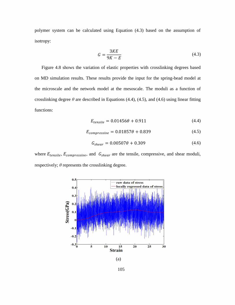
105
polymer system can be calculated using Equation (4.3) based on the assumption of
isotropy:
(4.3)
Figure 4.8 shows the variation of elastic properties with crosslinking degrees based
on MD simulation results. These results provide the input for the spring-bead model at
the microscale and the network model at the mesoscale. The moduli as a function of
crosslinking degree θ are described in Equations (4.4), (4.5), and (4.6) using linear fitting
functions:
(4.4)
(4.5)
(4.6)
where , , and are the tensile, compressive, and shear moduli,
respectively; θ represents the crosslinking degree.
(a)
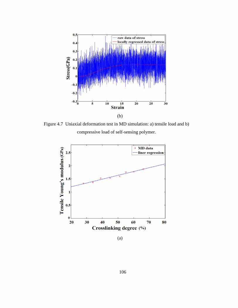
106
(b)
Figure 4.7 Uniaxial deformation test in MD simulation: a) tensile load and b)
compressive load of self-sensing polymer.
(a)

107
(b)
(c)
Figure 4.8 Relationship between crosslinking degrees and a) tensile modulus, b)
compressive modulus and c) shear modulus.

108
4.3. Development of spring-bead model to represent bond clusters at the microscale
Micromechanical techniques allow the mechanical behavior of polymers to be
analyzed through the continuum approximation of heterogeneous microstructures. The
variation of microstructural properties leads to variable macroscopic properties. Because
the mechanical behavior in nanocomposites is affected more by discrete phenomena, the
application of continuum mechanics is not a suitable option at the microscale. The FE
method is the most widely used numerical methods for discretizing the continuum
mechanical description of a material (Buxton, 2002). The FE method incorporates a
complex preprocessed mesh which allows detailed investigations of complex geometries
at hot spots, while enabling complex constitutive relations to be incorporated. However,
the accuracy and efficiency of FE method are dependent on mesh sizes, and therefore
limitations exist on the level of complexity that can be simulated (Tomar, 2004). In order
to simulate more heterogeneous microstructures, a simpler technique may be adopted.
The spring-bead model is considered as a two-dimensional or three-dimensional network
of interconnecting one-dimensional linear springs. The continuous material is lumped
into discrete beads. The neighbor springs are linked together by the nodes fastened in the
centers of the beads. The principal advantages of the model are the ease with which the
microstructural heterogeneity can be incorporated through the local variation in spring
characteristics, and the simulation of crack propagation through the iterative removal of
springs.
In this work a spring-bead model is developed to characterize the elastic deformation
of a crosslinked cluster of polymer chains with inputs from MD simulations that define

109
local material properties. At each iteration step in the simulation, forces in the springs are
applied to the nodes at the center of the beads, and the equilibrated nodal displacements
throughout the system are calculated. Different from the traditional FE method for
obtaining stress and strain, the spring-bead model provides the displacements of the
nodes and forces in the springs. The equivalent strain and strain energy of spring-bead
based network model can be defined and calculated using the displacements of nodes and
the spring characteristics. Furthermore, the results from the network model can be scaled
up to obtain the structural response at the macroscale using FE analysis (see Figure 4.1).
In this spring-bead model (see Figure 4.9 (a)), each of the two beads serves as half of
the mass of the bond cluster; the linear spring is used to represent the mechanical
response (tensile and compressive) of the bond cluster, and the potential energy stored in
the spring due to extension or compression captures the elastic strain energy in the
deformed material. The spring-bead model can be further simplified as shown in Figure
4.9 (b), where the spring is replaced by a line with linear force-extension behavior. The
relation between the force and relative displacement is shown in Figure 4.9 (c). Variable
spring stiffness (ratios of force to relative displacement) is used to represent bond clusters
with different crosslinking degrees. It should be noted that the architecture of this spring-
bead model is dependent on the size of the bond cluster. To represent a bond cluster with
a larger size, the mass of beads will be enhanced, and the spring stiffness will be
increased as well. The linear relation between force and relative displacement can be
expressed in Equation (4.7):
∆ (4.7)

110
where, F is the attractive/exclusive force in the spring, ∆ is the relative displacement of
the two beads compared to their original state, and k represents the spring stiffness. The
elastic energy stored in the spring can be expressed as:
∆ (4.8)
where, E is the elastic energy stored in the spring. The elastic energy is used to calculate
the equivalent strain energy density of the network model.
The existing set-up of the spring-bead model can be extended to characterize the
elastic-plastic material behavior by replacing the linear springs with appropriate nonlinear
ones. Dampers can also be added in the spring-bead model to represent the viscoelastic
and viscoplastic properties of some materials. However, experimental tensile tests of the
self-sensing polymer material exhibit brittle behavior. There is no obvious plasticity
region observed from these experimental tensile tests. Therefore, the spring-bead model
and the subsequent network model developed in this study use linear springs to capture
the mechanical response of the self-sensing polymer.
a)
b) c)
Figure 4.9 a) Spring-bead model; b) simplified spring-bead model; c) mechanical

111
response of spring-bead models with different crosslinking degrees.
4.4. Development of network model at the mesoscale
The spring-bead model can only carry load in the uniaxial direction of the spring. At
each point in the amorphous polymer material, there should be tensile, compressive, and
shear load carrying ability in all directions. Therefore, it is important that the network
model with crosslinked springs and beads accurately represents the load carrying capacity
in all directions. The construction, evaluation and the parametric studies of different
network models are discussed in this section. Different kinds of network models, named
according to the number of neighbor beads surrounding each bead (i.e., a 6 neighbor
based network model implies that each bead is connected with six neighbor beads using
springs), are designed and compared. The network model, consisting of a series of beads
and springs connected to neighboring beads, is used to represent larger crosslinked
polymer chains and capture the omnidirectional mechanical responses of the material. In
addition, the network model serving as a simplified mechanical equivalent of MD
simulations leads to significant reduction in computational resources compared to MD
simulations.
Different combinations of spring-bead arrangements are studied to understand the
mechanical behavior of the material. Several combination strategies (including 3, 4, 6, 8,
and 12 neighbor based connections) are shown in Figure 4.10. The bead located at the
center of the grey area is used to represent the total mass of the corresponding area. The
spring stiffness is equivalent to the strength of the related bond cluster calculated from
MD simulation. In the candidate network models, the spring length is defined as 0.8 μm;
this value is also used as the lower bound if there is more than one kind of spring. For

112
example, there are two kinds of springs for 8 neighbor based network model (see 4.10d).
The short spring length is defined as 0.8 μm in the 8 neighbor based network model. The
density of springs and beads in the network models are listed in Table 4.2. It must be
noted that complex network models with more neighbors will reduce simulation
efficiency; therefore network models with more than 12 neighbors are not considered in
this approach.
a) b)
c) d) e)
Figure 4.10 Different arrangements of spring-bead models to form a: a) 3 neighbor based;
b) 4 neighbor based; c) 6 neighbor based; d) 8 neighbor based; e) 12 neighbor based
network model.
The candidate network models are listed in Figure 4.10. The optimal arrangement is
the one that is capable of carrying tensile, compressive, and shear loads. Among the
candidate combinations, the 3 and 4 neighbor based models are not stable structures
because they do not exhibit shear load carrying capacity. For the remaining three

113
candidate network models shown in Figure 4.11 (6, 8, and 12 neighbor based
arrangements), the optimized configuration is evaluated by how well a candidate model
can represent the mechanical response at the mesoscale.
a) b)
c)
Figure 4.11 The 6, 8, and 12 neighbor based network models
The self-sensing polymer is assumed to be homogeneous and isotropic at the
mesoscale and macroscale. Therefore, the representation of isotropic property is
considered to be an important criterion for evaluating the optimal network configuration.
In all the network models proposed above, the springs are aligned along specific
directions, depending on the type of the network configuration. For example, in the 8
neighbor based network model (see figure 4.11b), all the springs are at an angle of 0°,

114
45°, 90°, or 135°. Consequently, the mechanical response of all combined network
models is dependent on orientations.
A 6 neighbor based network model is constructed with springs of uniform length
whereas the 8 and the 12 neighbor based network models are made up of two types of
springs (long and short). Since changes in the spring stiffness will lead to different
mechanical properties, the polymer material at different crosslinking degrees can be
represented effectively by appropriately varying the k1 (long spring) or k2 (short spring)
values. This feature provides the possibility of generating an equivalent isotropic network
model using a specific ratio of spring stiffness. Additionally, an isotropy index is defined
to describe the orientation-dependence of mechanical property in the network model:
where, represents Young‘s modulus in the principal direction (x-direction of the
network model in Figure 4.11), E( ) represents the Young‘s modulus along an arbitrary
direction at an angle with respect to the x-direction, is the isotropy index that
shows the variation of material property along different directions. For a perfectly
isotropic material, the isotropy index is equal to 1. An isotropic index approaching
unity is indicative of good isotropic material property representation.
The evaluations of candidate network models are listed in Table 2. The 6 neighbor
based network model fails to represent good isotropic property because it uses a single
spring configuration; the average isotropy index of a 6 neighbor based network model is
1.149 and the root mean square deviation (RMSD) between different directions is 7.45%.
(4.9)

115
For the 8 and the 12 neighbor based network models, a parametric approach was adopted
to find the relation between the RMSD of mechanical property in different directions and
the stiffness ratio of long springs to short springs. From the simulation results, it can be
observed that the average isotropy index is a continuously increasing function of stiffness
ratio of springs. For the 8 neighbor based network model, the RMSD is 0.04% when the
stiffness ratio is 0.6002 (see Figure 4.12a). The maximum difference between mechanical
properties along different directions is 0.08%. For the 12 neighbor based configuration,
the minimum isotropy index is 1.149 and the RMSD value is 7.45%. Therefore, the 12
neighbor based network model cannot adequately represent the isotropic property.
a) b)
Figure 4.12 Isotropic representation of a) 8 neighbor based, and b) 12 neighbor based
network models corresponding to stiffness ratio of long spring to short spring.
To summarize the results in this section, the 3 and the 4 neighbor based network
models cannot carry loads owing to their unstable structures, whereas the 6 and the 12
neighbor based network models lack good isotropic representation capability. In addition,

116
the 12 neighbor based network model consists of a high number of springs and beads,
which will increase simulation time and cost. The 8 neighbor based network model is the
optimal one considering structural stability, representation of isotropic property, and
computational efficiency. The 8 neighbor based network model is equivalently isotropic
when the ratio of long spring stiffness k2 to short spring stiffness k1 is given as 0.6002. It
must be noted that a 2D spring-bead based network model represents a polymer plate of
unit thickness (1 μm). The spring stiffness will be redefined by multiplying a factor (ratio
of material thickness to 1 μm) to represent different material thickness.
Table 4.2 Configuration and evaluation of network models with different combination
methods.
Network
model
Number of
beads per 100
μm2
Number of
springs per 100
μm2
Evaluation Optimal
isotropic index
3 neighbors 120 181 Not stable Not applicable
4 neighbors 156 313 Not stable Not applicable
6 neighbors 180 541 Anisotropic 1.1490
8 neighbors 156 625 Optimal model 1.0008
12 neighbors 180 1081 Anisotropic 1.1490
4.5. Optimization of mechanical equivalence between MD model and network
model
The network model integrated results from molecular level simulations to the
mesoscale. Mechanical equivalence of the network model with the actual MD system
also validates the approximation at the microscale. The next step is to determine the
spring strengths that ensure minimal deviation of the mechanical properties obtained
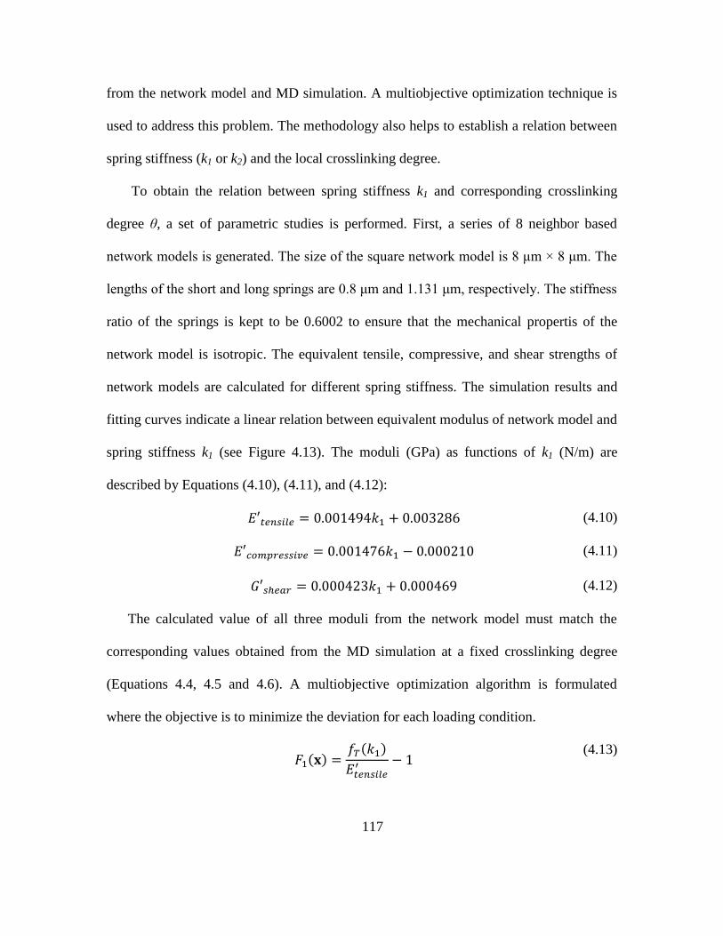
117
from the network model and MD simulation. A multiobjective optimization technique is
used to address this problem. The methodology also helps to establish a relation between
spring stiffness (k1 or k2) and the local crosslinking degree.
To obtain the relation between spring stiffness k1 and corresponding crosslinking
degree θ, a set of parametric studies is performed. First, a series of 8 neighbor based
network models is generated. The size of the square network model is 8 μm × 8 μm. The
lengths of the short and long springs are 0.8 μm and 1.131 μm, respectively. The stiffness
ratio of the springs is kept to be 0.6002 to ensure that the mechanical propertis of the
network model is isotropic. The equivalent tensile, compressive, and shear strengths of
network models are calculated for different spring stiffness. The simulation results and
fitting curves indicate a linear relation between equivalent modulus of network model and
spring stiffness k1 (see Figure 4.13). The moduli (GPa) as functions of k1 (N/m) are
described by Equations (4.10), (4.11), and (4.12):
(4.10)
(4.11)
(4.12)
The calculated value of all three moduli from the network model must match the
corresponding values obtained from the MD simulation at a fixed crosslinking degree
(Equations 4.4, 4.5 and 4.6). A multiobjective optimization algorithm is formulated
where the objective is to minimize the deviation for each loading condition.
(4.13)

118
(4.14)
(4.15)
It must be noted that the objectives are competing as well as coupled; i.e., the design
variable, k1, has a different degree of impact on each of the three objective functions, and
the minimization of one objective could lead to an increase in the value of another
objective. Therefore, a robust technique is required to determine the optimal spring
stiffness at each crosslinking degree. The Kreisselmeier-Steinhauser (KS) function
approach is used to solve the multiobjective optimization problem. Using the KS
function, a composite envelope function is formulated to transform the original multiple
objectives and constraints to a single unconstrained objective function (Chattopadhyay,
1991, 1994). The first step in formulating the objective function in this approach involves
the transformation of the original objective functions into reduced objective functions.
The reduced objective functions are of the form:
(4.16)
where, Fk0 corresponds to the value of Fk calculated at the start of each iteration; ‗gmax‘ is
the maximum value among all the constraints and remains constant throughout the
iteration. The KS function combines the objectives and constraints (nobj + m = M) to form
the single objective function, described in Equation (4.17):
∑
(4.17)

119
The algorithm attempts to satisfy the constraints of the reduced objective function by
maximizing Fk. The multiplier ―ρ‖ is analogous to the draw-down parameter of penalty
function formulations and controls the distance from the surface of the KS objective
function to the surface of the maximum function value. A large value of ‗ρ‘ causes the
KS function to closely follow the surface of the largest constraint function; a small value
causes the inclusion of violated constraints to the KS function (Haftka, 1992).
a)

120
b)
c)
Figure 4.13 Fitting curves of modulus as a function of spring stiffness: a) tensile
modulus; b) compressive modulus; c) shear modulus.

121
Figure 4.14 compares the performance of the optimization algorithm with respect to
the results from MD simulation. The optimal k1 value overestimates the values of the
tensile and compressive moduli at lower crosslinking degrees. However, at the most
likely crosslinking degree (~ 52.72%), which is the average crosslinking degree in the
500 MD simulations, the error between the tensile and the compressive responses are
quite balanced. The norm of the maximum constraint violation is within the specified
tolerance of 1×10⁻⁴
.
Figure 4.14 Comparison between MD simulation and optimization results.

122
Figure 4.15 Linear fitting curve of spring stiffness based on optimization results.
Figure 4.15 illustrates the variation of optimal spring stiffness with crosslinking
degree. The relationship is a close linear approximation; this result is consistent with the
inference from MD simulation that the tensile, compressive, and shear moduli vary
linearly with crosslinking degree. The linear fitting expression of the optimal spring
stiffness k1 using the crosslinking degree θ is shown in Equation (4.18):
(4.18)
4.6. Equivalent strain and strain energy in network model
The network model is constructed by crosslinked springs and discrete beads, instead
of continuous material. Therefore the traditional concepts of strain and strain energy
density are not available for this modeling. New concepts of strain and strain energy are
required before the discussion and evaluation of network model in next chapter. In
traditional continuous materials, strain is defined as a geometrical measure of
deformation representing the relative displacement between particles in a material body.

123
In spring-bead based network model, the ―equivalent strain‖ in one spring is defined as
the deformation in term of original and relative displacement between the two beads
linked by this spring, as shown in Equation (4.19):
‖
∆
‖
(4.19)
where, is the original length of the ith spring, ∆ is the change of the same spring
length, and is the equivalent strain of the ith spring. For each bead in the 8 neighbor
based network model, there are eight beads linked to it directly using springs (see Figure
4.16). The averaged equivalent strain in the bead centered subzone (the grey square zone
in Figure 4.16) is defined as the averaged value of the strain in the eight neighbor springs
linking to the centered bead. For the 8 neighbor based network model, the length of the
square subzone side is equal to the shorter spring length. The equivalent strain in the
subzone is defined as:
∑
(4.20)
where is the equivalent strain in the ith spring, which is defined in equation (4.19), is
the averaged equivalent strain in the subzone (grey zone in Figure 4.16), and N is the
number of neighbor springs linked to the center bead. For the 8 neighbor based network
model, N is equal to 8.
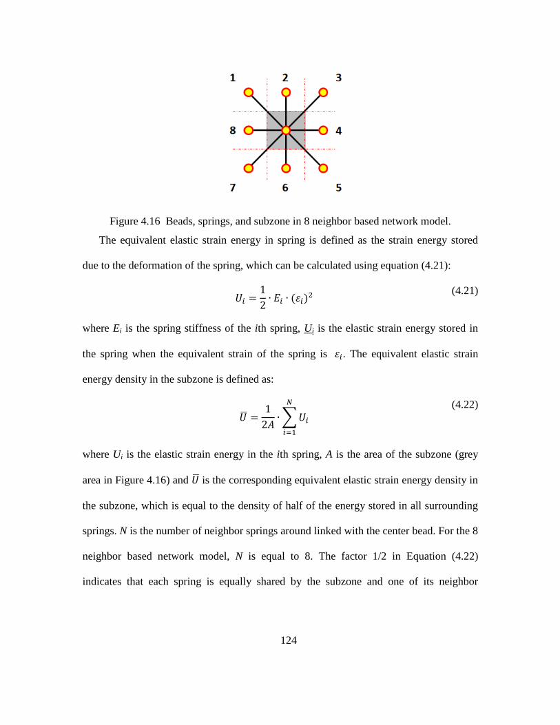
124
Figure 4.16 Beads, springs, and subzone in 8 neighbor based network model.
The equivalent elastic strain energy in spring is defined as the strain energy stored
due to the deformation of the spring, which can be calculated using equation (4.21):
(4.21)
where Ei is the spring stiffness of the ith spring, Ui is the elastic strain energy stored in
the spring when the equivalent strain of the spring is . The equivalent elastic strain
energy density in the subzone is defined as:
∑
(4.22)
where Ui is the elastic strain energy in the ith spring, A is the area of the subzone (grey
area in Figure 4.16) and is the corresponding equivalent elastic strain energy density in
the subzone, which is equal to the density of half of the energy stored in all surrounding
springs. N is the number of neighbor springs around linked with the center bead. For the 8
neighbor based network model, N is equal to 8. The factor 1/2 in Equation (4.22)
indicates that each spring is equally shared by the subzone and one of its neighbor

125
subzones. So the total elastic strain energy in each spring is divided into two equal parts
in the calculation of the equivalent strain energy density.
4.7. Summary
In this chapter, a spring-bead based network model was developed to represent the
mechanical properties of self-sensing polymeric material. At the microscale, the spring-
bead model was developed to represent mechanical properties and mass of cluster bonds.
MD simulation was implemented to provide necessary information to construct the
spring-bead model. At the mesoscale, a computationally efficient network model was
developed; these models were implemented in a general purpose finite element solver to
obtain the mechanical properties. Parametric studies and multiobjective optimization
were conducted to construct an optimal combination of an 8 neighbor based network
model and determine the corresponding spring stiffness. Compared to MD simulations,
the spring-bead based network model can significantly improve the simulation efficiency
while maintaining sufficient accuracy.

126
5. Multiscale Modeling of Self-sensing Polymer using
Statistical Network Model
5.1. Background
Discrete material techniques, such as the spring-bead based network model, have
been developed to study polymer material (Iwata, 2003; Schwarz, 2006; Indei, 2012).
Spring-bead chains are crosslinked to generate the network model to represent the larger
scale material behavior of polymer. In epoxy based self-sensing polymers the
crosslinking bond clusters between the resin and the hardener molecules generate a larger
scale of network structure. The heterogeneous crosslinked microstructure at the
microscale has significant effect on the local mechanical properties (Flory, 1943;
Krumova, 2000; Fan, 2007). Therefore to design and synthesize polymers with
multifunctional capabilities it is important to develop a fundamental understanding of the
effects of nano- and microscale variability on material properties and response such as
Young‘s modulus, heterogeneous stress/strain distribution and damage precursor.
Parametric studies of the variability, such as the crosslinking degree, chain flexibility and
chain length, are important to enhance the accuracy of the network models (Espuche,
1995; Chzarulatha, 2003; Park, 2006) discussed in Chapter 4. Among all variability the
crosslinking degree (or crosslinking density), which represents the degree of microscopic
covalent bonds, plays an important role in influencing the mechanical properties (Zosel,
1993; Espuche, 1995; Halary, 2000; Berger, 2004). In this research the computationally
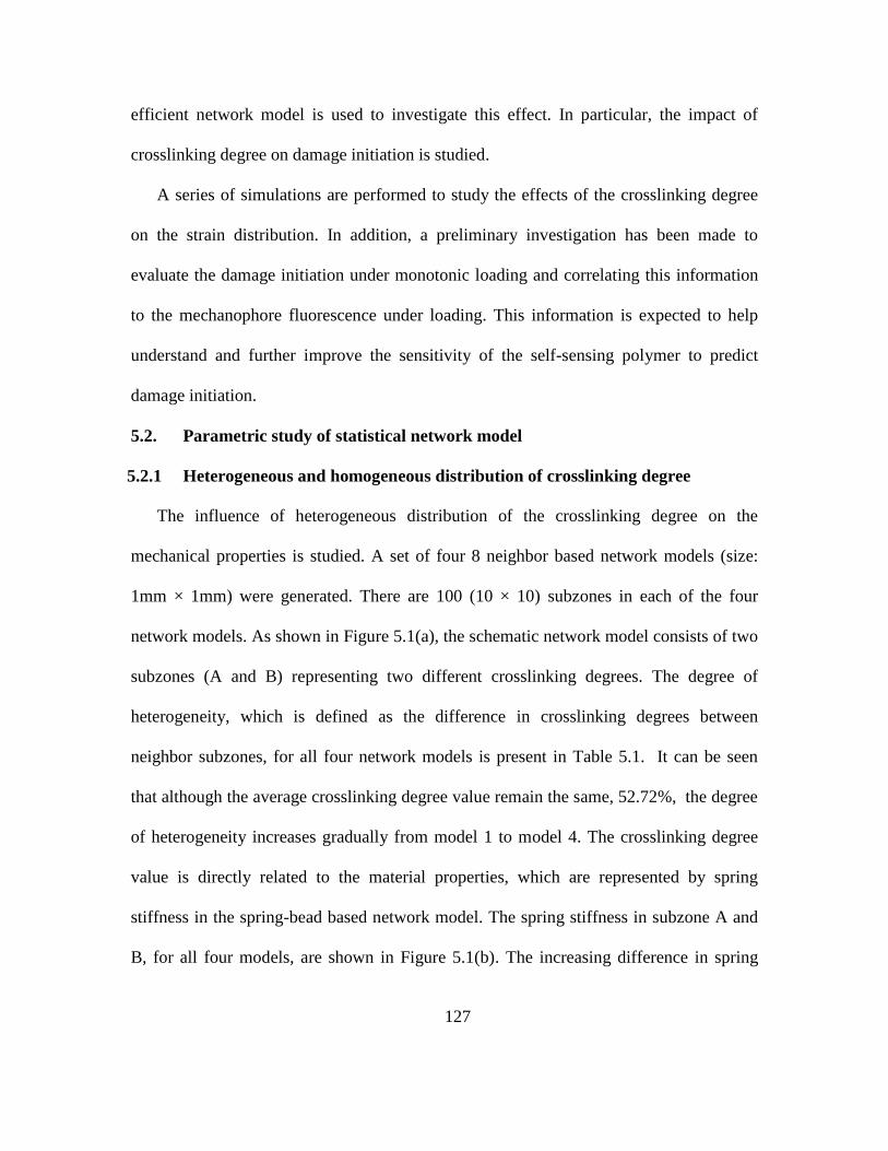
127
efficient network model is used to investigate this effect. In particular, the impact of
crosslinking degree on damage initiation is studied.
A series of simulations are performed to study the effects of the crosslinking degree
on the strain distribution. In addition, a preliminary investigation has been made to
evaluate the damage initiation under monotonic loading and correlating this information
to the mechanophore fluorescence under loading. This information is expected to help
understand and further improve the sensitivity of the self-sensing polymer to predict
damage initiation.
5.2. Parametric study of statistical network model
5.2.1 Heterogeneous and homogeneous distribution of crosslinking degree
The influence of heterogeneous distribution of the crosslinking degree on the
mechanical properties is studied. A set of four 8 neighbor based network models (size:
1mm × 1mm) were generated. There are 100 (10 × 10) subzones in each of the four
network models. As shown in Figure 5.1(a), the schematic network model consists of two
subzones (A and B) representing two different crosslinking degrees. The degree of
heterogeneity, which is defined as the difference in crosslinking degrees between
neighbor subzones, for all four network models is present in Table 5.1. It can be seen
that although the average crosslinking degree value remain the same, 52.72%, the degree
of heterogeneity increases gradually from model 1 to model 4. The crosslinking degree
value is directly related to the material properties, which are represented by spring
stiffness in the spring-bead based network model. The spring stiffness in subzone A and
B, for all four models, are shown in Figure 5.1(b). The increasing difference in spring

128
stiffness between neighbor subzones also indicates that the material properties changes
from homogeneous to heterogeneous.
a) b)
Figure 5.1 a) Specific network model to study effect of degree of heterogeneity and b)
spring stiffness in subzone A and B of the network model 1, 2, 3 and 4.
Table 5.1 crosslinking degree and degree of heterogeneity in the four network models
crosslinking degree in A crosslinking degree in B Heterogeneous degree
Model 1 52.72% 52.72% 0
Model 2 51.72% 53.72% 2%
Model 3 50.72% 54.72% 4%
Model 4 49.72% 55.72% 6%
Simulations were conducted using uniaxial tensile load applied to all four network
models. The loading was strain control and the maximum loading strain was 5%. The
average equivalent strain which is defined as the average deformation of springs in one
subzone is used to evaluate the strain in the network models. The simulation results are
shown in Table 5.2 and Figure 5.2. In model 1, 2, and 3, where the degree of
heterogeneity is not more than 4%, the average equivalent strain is nearly the same (equal
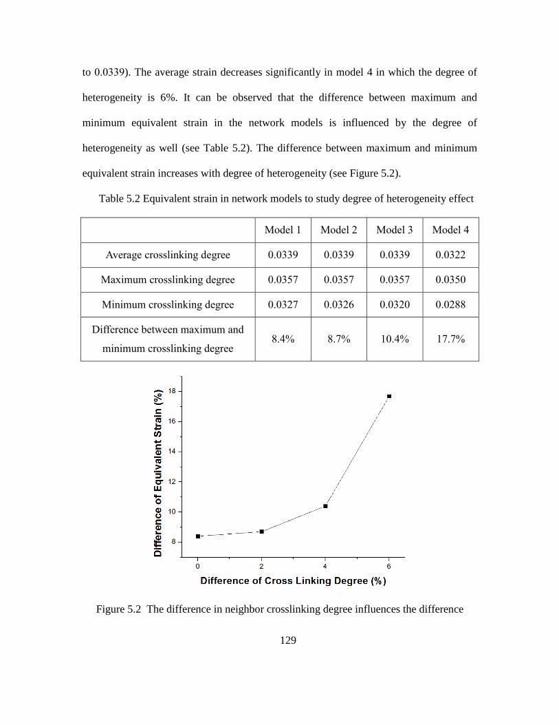
129
to 0.0339). The average strain decreases significantly in model 4 in which the degree of
heterogeneity is 6%. It can be observed that the difference between maximum and
minimum equivalent strain in the network models is influenced by the degree of
heterogeneity as well (see Table 5.2). The difference between maximum and minimum
equivalent strain increases with degree of heterogeneity (see Figure 5.2).
Table 5.2 Equivalent strain in network models to study degree of heterogeneity effect
Model 1 Model 2 Model 3 Model 4
Average crosslinking degree 0.0339 0.0339 0.0339 0.0322
Maximum crosslinking degree 0.0357 0.0357 0.0357 0.0350
Minimum crosslinking degree 0.0327 0.0326 0.0320 0.0288
Difference between maximum and
minimum crosslinking degree 8.4% 8.7% 10.4% 17.7%
Figure 5.2 The difference in neighbor crosslinking degree influences the difference
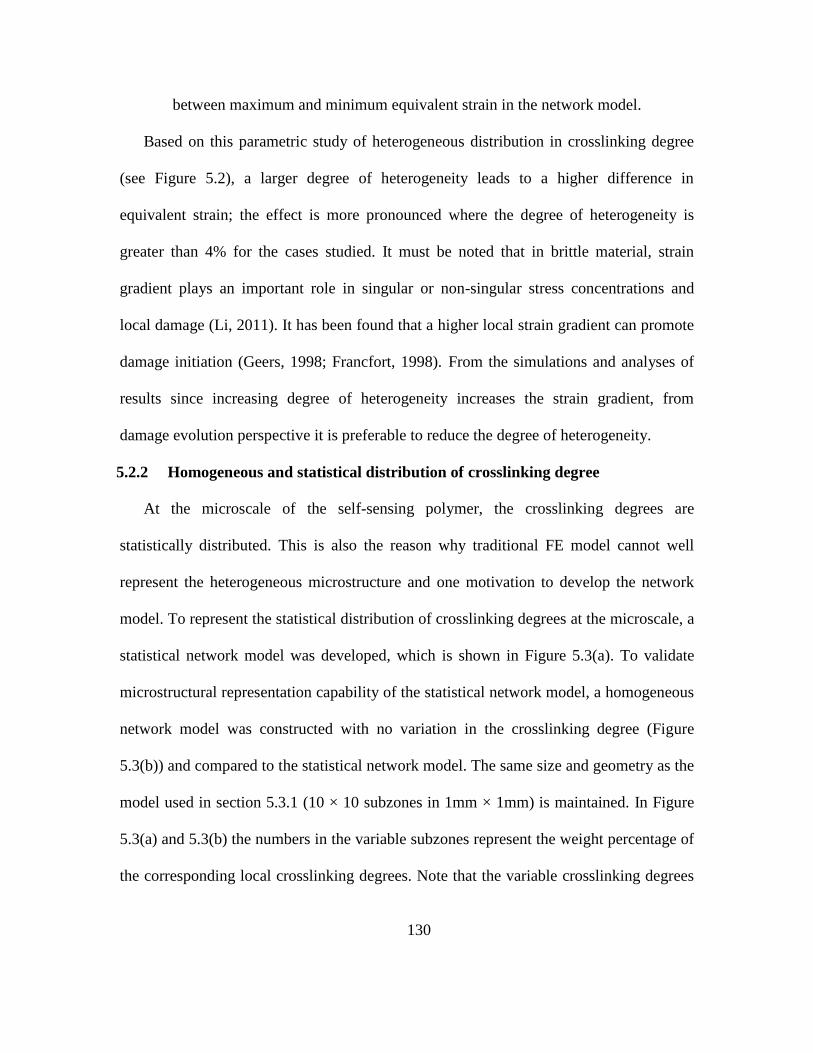
130
between maximum and minimum equivalent strain in the network model.
Based on this parametric study of heterogeneous distribution in crosslinking degree
(see Figure 5.2), a larger degree of heterogeneity leads to a higher difference in
equivalent strain; the effect is more pronounced where the degree of heterogeneity is
greater than 4% for the cases studied. It must be noted that in brittle material, strain
gradient plays an important role in singular or non-singular stress concentrations and
local damage (Li, 2011). It has been found that a higher local strain gradient can promote
damage initiation (Geers, 1998; Francfort, 1998). From the simulations and analyses of
results since increasing degree of heterogeneity increases the strain gradient, from
damage evolution perspective it is preferable to reduce the degree of heterogeneity.
5.2.2 Homogeneous and statistical distribution of crosslinking degree
At the microscale of the self-sensing polymer, the crosslinking degrees are
statistically distributed. This is also the reason why traditional FE model cannot well
represent the heterogeneous microstructure and one motivation to develop the network
model. To represent the statistical distribution of crosslinking degrees at the microscale, a
statistical network model was developed, which is shown in Figure 5.3(a). To validate
microstructural representation capability of the statistical network model, a homogeneous
network model was constructed with no variation in the crosslinking degree (Figure
5.3(b)) and compared to the statistical network model. The same size and geometry as the
model used in section 5.3.1 (10 × 10 subzones in 1mm × 1mm) is maintained. In Figure
5.3(a) and 5.3(b) the numbers in the variable subzones represent the weight percentage of
the corresponding local crosslinking degrees. Note that the variable crosslinking degrees
131
in the statistical network model isrned by the probability density function (PDF) obtained
from the MD simulation (see Figure 4.6). For the homogeneous network model, uniform
crosslinking degree which is equal to the averaged value of all crosslinking degrees in the
statistical network model (52.72%) is used for all subzones.
a) b)
Figure 5.3 Crosslinking degree distribution in a) statistical network model and b)
homogeneous network model (unit: %).
Uniaxial tensile test was performed in both statistical and homogeneous network
models. The loading was strain control and the maximum loading strain was 5%. The
simulation results are shown in Figure 5.4(a) and 5.4(b), which provide the equivalent
strain distribution in the statistical and homogeneous network models, respectively.
Results of the average, maximum and minimum equivalent strain in the statistical and
homogeneous network models are presented in Table 5.3.

132
a) b)
Figure 5.4 Equivalent strain distribution in a) statistical network model and b)
homogeneous network model.
As shown in Table 5.3, the average values of equivalent strain in statistical network
model and homogeneous network model are close. This implies that the overall
mechanical property of the statistical network model corresponds well with the
homogeneous model under monotonic loading. The difference between maximum and
minimum strain for statistical network model (which is 10.36%) is greater than the
corresponding value for homogeneous network model (which is 8.40%). This observation
implies that the statistical distribution of crosslinking degrees results in a larger
distinguishable disorder in strain distribution; indicating that there is a high strain
gradient. This increase in strain gradient can lead to early damage initiation in the
homogeneous microstructure.
Table 5.3 Equivalent strain in statistical and homogeneous network models
Equivalent Statistical Homogeneous
Average 0.0338 0.0339
Maximum 0.0357 0.0357
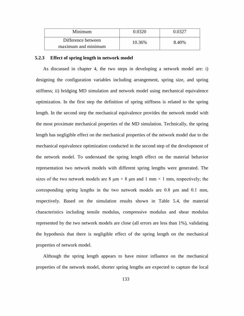
133
Minimum 0.0320 0.0327
Difference between
maximum and minimum 10.36% 8.40%
5.2.3 Effect of spring length in network model
As discussed in chapter 4, the two steps in developing a network model are: i)
designing the configuration variables including arrangement, spring size, and spring
stiffness; ii) bridging MD simulation and network model using mechanical equivalence
optimization. In the first step the definition of spring stiffness is related to the spring
length. In the second step the mechanical equivalence provides the network model with
the most proximate mechanical properties of the MD simulation. Technically, the spring
length has negligible effect on the mechanical properties of the network model due to the
mechanical equivalence optimization conducted in the second step of the development of
the network model. To understand the spring length effect on the material behavior
representation two network models with different spring lengths were generated. The
sizes of the two network models are 8 μm × 8 μm and 1 mm × 1 mm, respectively; the
corresponding spring lengths in the two network models are 0.8 μm and 0.1 mm,
respectively. Based on the simulation results shown in Table 5.4, the material
characteristics including tensile modulus, compressive modulus and shear modulus
represented by the two network models are close (all errors are less than 1%), validating
the hypothesis that there is negligible effect of the spring length on the mechanical
properties of network model.
Although the spring length appears to have minor influence on the mechanical
properties of the network model, shorter spring lengths are expected to capture the local
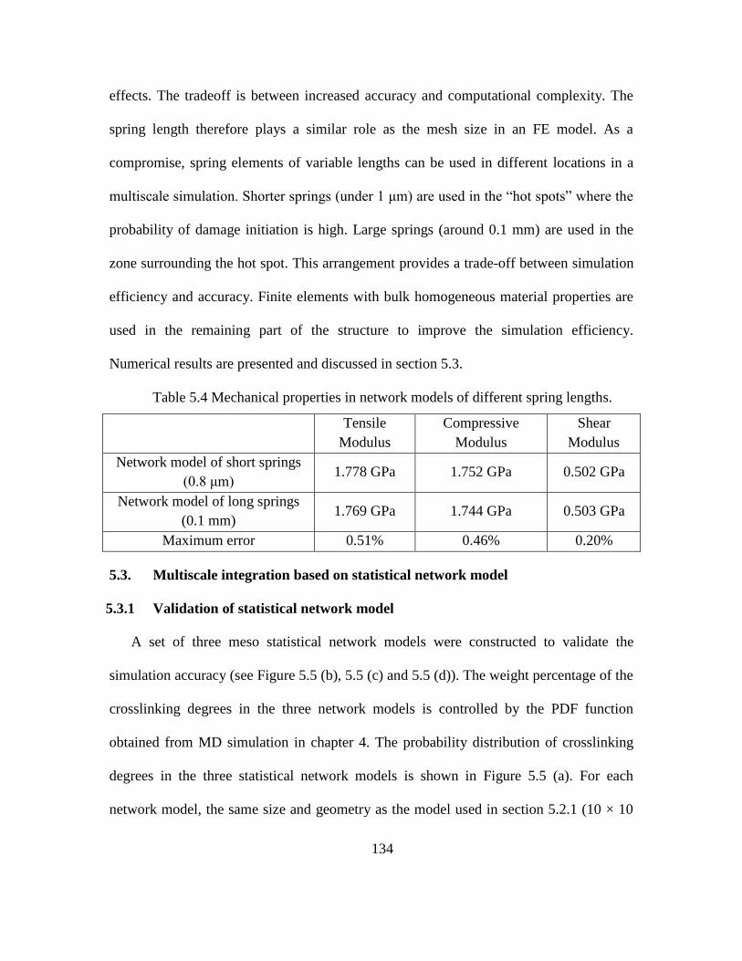
134
effects. The tradeoff is between increased accuracy and computational complexity. The
spring length therefore plays a similar role as the mesh size in an FE model. As a
compromise, spring elements of variable lengths can be used in different locations in a
multiscale simulation. Shorter springs (under 1 μm) are used in the ―hot spots‖ where the
probability of damage initiation is high. Large springs (around 0.1 mm) are used in the
zone surrounding the hot spot. This arrangement provides a trade-off between simulation
efficiency and accuracy. Finite elements with bulk homogeneous material properties are
used in the remaining part of the structure to improve the simulation efficiency.
Numerical results are presented and discussed in section 5.3.
Table 5.4 Mechanical properties in network models of different spring lengths.
Tensile
Modulus
Compressive
Modulus
Shear
Modulus
Network model of short springs
(0.8 μm) 1.778 GPa 1.752 GPa 0.502 GPa
Network model of long springs
(0.1 mm) 1.769 GPa 1.744 GPa 0.503 GPa
Maximum error 0.51% 0.46% 0.20%
5.3. Multiscale integration based on statistical network model
5.3.1 Validation of statistical network model
A set of three meso statistical network models were constructed to validate the
simulation accuracy (see Figure 5.5 (b), 5.5 (c) and 5.5 (d)). The weight percentage of the
crosslinking degrees in the three network models is controlled by the PDF function
obtained from MD simulation in chapter 4. The probability distribution of crosslinking
degrees in the three statistical network models is shown in Figure 5.5 (a). For each
network model, the same size and geometry as the model used in section 5.2.1 (10 × 10

135
subzones in 1mm × 1mm) is maintained. There are 121 beads, 220 short springs, and 200
long springs in the 8 neighbors based network model. The lengths of the short and long
springs in the network models are 0.1 mm and 0.1414 mm respectively. The numbers
shown on the square subzones in Figure 5.5 (b), 5.5 (c), and 5.5 (d) represent the local
crosslinking degrees.
a) b)
c) d)

136
Figure 5.5 a) The probability distribution of crosslinking degree in the statistical
network model, b) network model 1, c) network model 2, and d) network model 3.
Simulations were conducted using uniaxial strain controlled tensile load; the
maximum loading strain was 10%. The average equivalent strain in the three network
models was calculated. It was observed that the average equivalent strain in the three
statistical network models was very close and the error was less than 1% (see Figure 5.6).
The results establish the validity and robustness of the representative models. It must be
noted that one deficiency of the developed network model is that it only captures the
mechanical properties, and does not take into account the thermal and chemical
properties of the mechanophores as in a MD simulation. This undoubtedly improves the
computational efficiency significantly. For a similar uniaxial tensile loading simulation
20 hours of runtime is required using MD modeling whereas a network model completes
the simulation in 4 minutes. The simulation efficiency is improved by 300 times using the
network model.

137
Figure 5.6 Average equivalent strain in three statistical network models v.s. loading
strain.
To validate the statistical network model, experimental investigations and their
correlations with the network model are discussed. Three statistical representative
network models were generated (see Figure 5.5 (b), (c) and (d)). A set of uniaxial
compressive experiments were performed to determine the Young‘s modulus of this self-
sensing material. An MTS Bionix 370.02 test frame (with the maximum loading
capability 22.2 kN) was used to conduct the compressive tests. The results from the
experiments and the simulations, shown in Table 5.4, show very good correlation in
Young‘s modulus prediction.
Table 5.5 Simulation and experimental results of Young‘s modulus
Model 1 Model 2 Model 3 Experiment
Young‘s modulus (GPa) 1.77 1.76 1.77 1.82

138
5.3.2 Local strain and crosslinking degree in the network model
Simulations were conducted with the statistical network model to study the relation
between local strain and crosslinking degree using biaxial strain controlled tensile load;
the maximum loading strain was 10% in both directions. The statistical network model 1
is used in the simulation (see Figure 5.7 (a)). The distribution of equivalent strain is
shown in Figure 5.7 (b). There is an obvious relation between local strain and
crosslinking degree: high strain concentration (the red band in Figure 5.7 (b)) occurs
mostly where there is low crosslinking degree (the red square zone in Figure 5.7 (a)),
especially in areas where the crosslinking degree is below 52.72%, which is the average
crosslinking degree in the model). These results are physically meaningful; lower
material stiffness leads to a higher strain under the same external loads. The locations
with high strain concentration also correlate to potential local defects. The damage
evaluation based on MD & network simulations will be discussed in section 5.4.
a) b)
Figure 5.7 Simulation of statistical network model under biaxial tensile load: a)
crosslinking degree distribution in network model and b) distribution of equivalent strain
in network model.
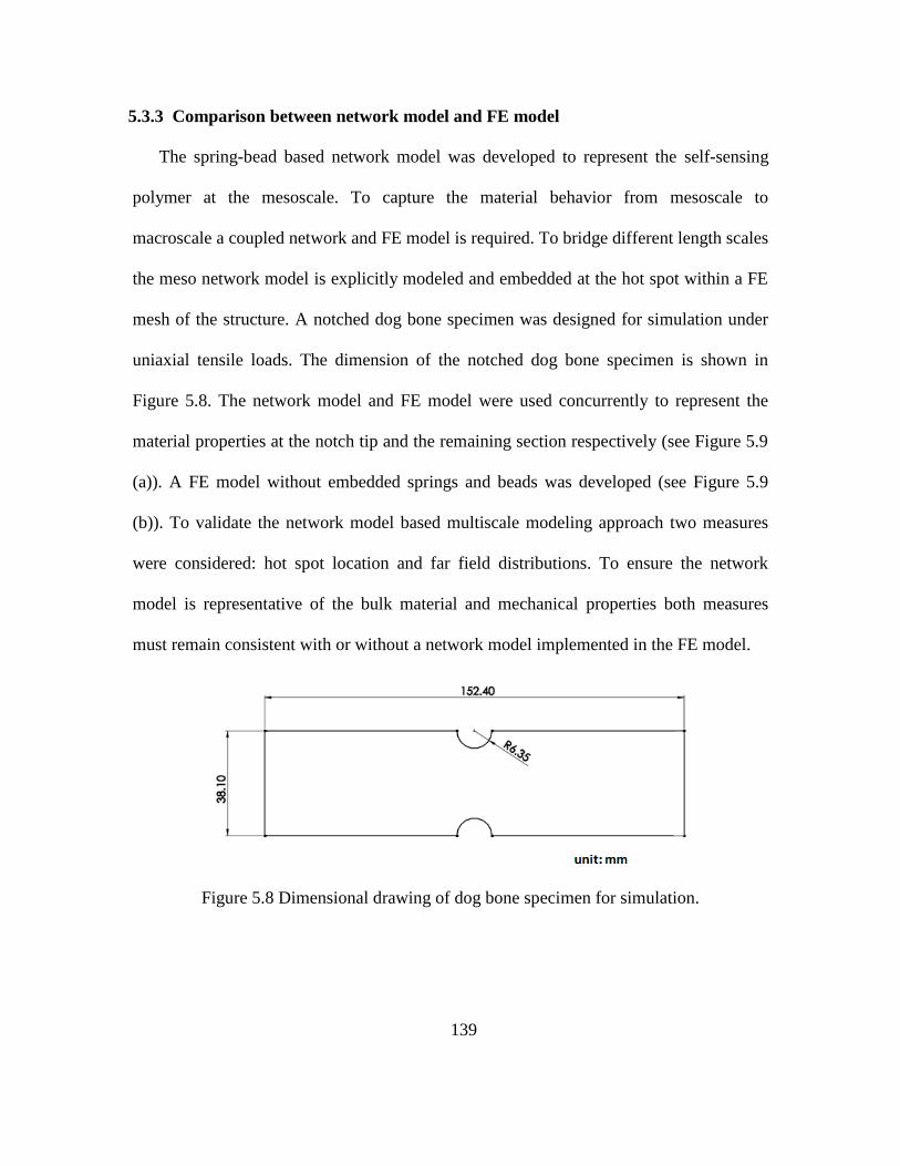
139
5.3.3 Comparison between network model and FE model
The spring-bead based network model was developed to represent the self-sensing
polymer at the mesoscale. To capture the material behavior from mesoscale to
macroscale a coupled network and FE model is required. To bridge different length scales
the meso network model is explicitly modeled and embedded at the hot spot within a FE
mesh of the structure. A notched dog bone specimen was designed for simulation under
uniaxial tensile loads. The dimension of the notched dog bone specimen is shown in
Figure 5.8. The network model and FE model were used concurrently to represent the
material properties at the notch tip and the remaining section respectively (see Figure 5.9
(a)). A FE model without embedded springs and beads was developed (see Figure 5.9
(b)). To validate the network model based multiscale modeling approach two measures
were considered: hot spot location and far field distributions. To ensure the network
model is representative of the bulk material and mechanical properties both measures
must remain consistent with or without a network model implemented in the FE model.
Figure 5.8 Dimensional drawing of dog bone specimen for simulation.

140
a) b)
Figure 5.9. Strain distribution in the hot spot using a) network model and b) FE
model.
Comparison of the strain distributions obtained using the two models are shown in
Figure 5.9. In both network model (Figure 5.9 (a)) and FE model (Figure 5.9 (b)) the high
strain concentrations are observed near the notch tip. However, the strain distribution in
the network model shows larger variability due to the variability in the crosslinking
degree. The local strain distribution obtained using the network model is expected to
provide more accurate estimate of the local defects at the microscale. Figure 5.10 (a) and
5.10 (b) show the comparison of strain distributions outside the hot spots in the
simulations, with and without a network model. The good correlation between network
model and FE model is observed, validating the accuracy of the network model with the
FE model outside of the hot spot (notch tip).

141
a) b)
Figure 5.10 Strain distribution within notched specimen a) with network model and b)
without network model.
5.4. Damage estimation using statistical network model
5.4.1 Evaluation of self-sensing intensity of smart polymer
In this research TCEs were used as stress-sensing particles to detect the defects in the
self-sensing polymer. The epoxy resins are brittle with a propensity to crack if exposed to
sufficient deformation, leading to irreversible damage in the form of micro cracking. In
the high strain concentration locations of the material the force can be transferred through
the bulk material to individual polymer chains, and then to the cleavable bonds on the
mechanophore units. The local deformation in these regions exceeds the critical
limitation of the polymer chains and results in the permanent deformation under rupture
of crosslinking bonds (Buehler, 2008). This early damage precursor can be detected
through the employment of TCE-containing polymers. Note that the fluorescence
response of the mechanophore results from the rupture of the covalent bonds in
cyclobutane. It is also related to the onset of permanent strain (deformation) of the bonds

142
at the microscale. The fluorescence intensity is also directly dependent on the density of
the breaking bonds. Therefore, there is a correlation between the local strain and the color
changing phenomena. This relation between fluorescence intensity obtained in the
experiments and the strain field predicted by in the simulation using the network model
was studied.
Uniaxial compressive tests were performed to obtain the fluorescence intensities of
the self-sensing material under different loads. A Test Resources Electromechanical
System (with the maximum loading capability 4.4 kN) was used to conduct the
compressive tests and the stress-strain curves were obtained. The tests were performed
with strain control in longitudinal direction at loading rate of 1 mm/min. The maximum
loading strain was 10% to ensure that the material remained in elastic stage. To monitor
the fluorescence from defects in the polymer the cubic samples of polymer blends were
compressed to different strains and observed under the fluorescence microscope (Nikon
Elipse TE300 inverted video microscope) by exposure to 330-380 nm UV light. An
image processing program, ImageJ, was used to process the fluorescent micrographs and
capture the fluorescence intensities. The micrographs were taken at the same location of
the specimen surface, with the size 427 μm × 325 μm. The integrated fluorescence
intensity was calculated through the summation of all pixel values in the image. A quasi-
linear relation was observed between the fluorescence intensity density and the loading
strain (see Figure 5.11 (a)). Figure 5.11 (b) and 5.11 (c) show the microscopic images of
the specimen surface and the corresponding fluorescence responses, when the loading

143
strain is 4% and 6% respectively. The relation between fluorescence intensity density and
the loading strain can be described using a linear fit:
(5.1)
where I represents the observed fluorescence intensity density, and is the loading strain.
b)
a) c)
Figure 5.11 Fluorescence observation of self-sensing polymer. a) Integrated intensity
density v.s. loading strain in fluorescence observation, b) Microscopic images and
detected fluorescence of specimen at 4% strain, and c) Microscopic images and
detected fluorescence of specimen at 6% strain.
Next, simulations were performed using statistical network model 1, as shown in
Figure 5.5(b). Uniaxial compressive loads of same magnitude were applied to the
network model. The equivalent strain in the network model was calculated and shows a
quasi-linear relation between the average equivalent strain and the loading strain (Figure
5.12 (a)). The distribution of equivalent strain in the network model under different
loading strain is shown in Figures 5.12 (b) - (e). The simulation result shows that the
strain distribution is influenced by the local crosslinking degree. Also, both local and
144
average equivalent strain increases linearly with loading. A linear fit is used to describe
the relation between average equivalent strain and global loading strain:
(5.2)
where is the loading strain, and is the average equivalent strain in the statistical
network model. As shown in Equations (5.1) and (5.2) both the fluorescence intensity and
the strain in the network model exhibit a quasi-linear relationship with respect to the
loading strain (see Figure 5.11(a) and Figure 5.12(a)). By combining Equation (5.1) and
(5.2), a relation between average strain in the network model and fluorescence intensity
density I from experimental observation can be obtained as follows.
169.09 +123.17 (5.3)
Equation (5.3) can be used as an indirect means to evaluate the observed fluorescence
intensity of the self-sensing material. Since the network model does not take into account
the chemical properties of the mechanopohore polymer, this simple strain based damage
index can be used to simulate the change in fluorescence intensity with increase in
mechanical strain.

145
a)
b)

146
c)
d)
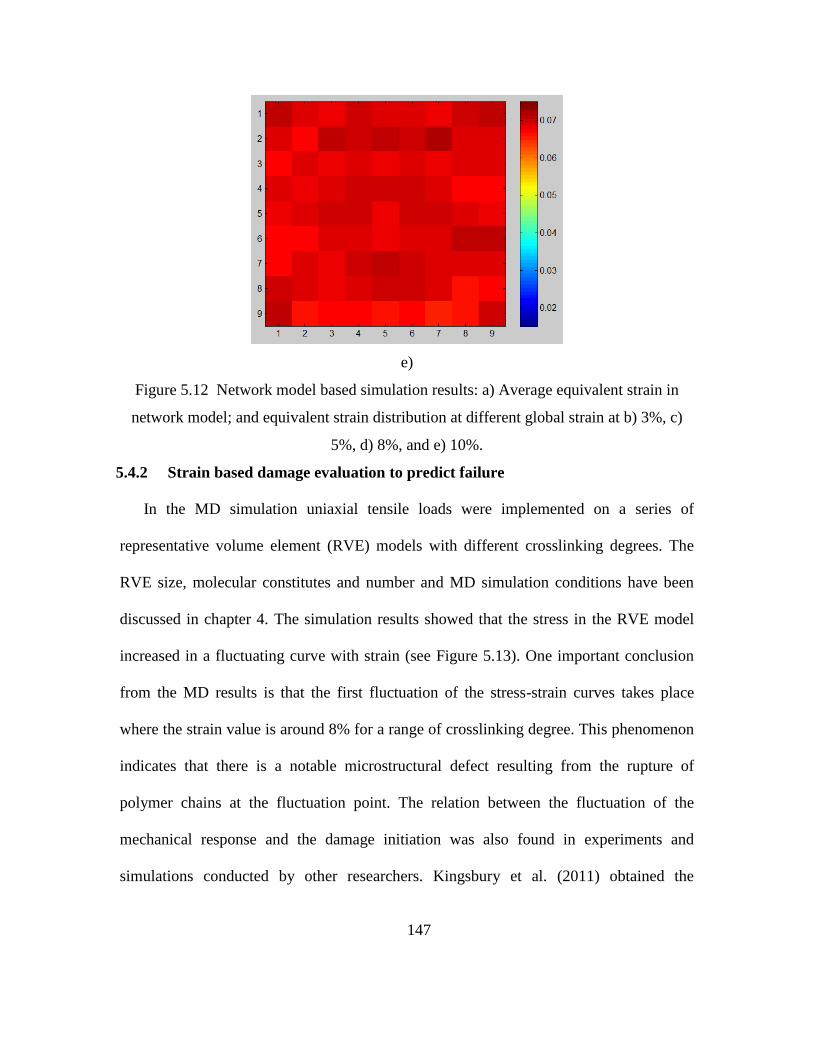
147
e)
Figure 5.12 Network model based simulation results: a) Average equivalent strain in
network model; and equivalent strain distribution at different global strain at b) 3%, c)
5%, d) 8%, and e) 10%.
5.4.2 Strain based damage evaluation to predict failure
In the MD simulation uniaxial tensile loads were implemented on a series of
representative volume element (RVE) models with different crosslinking degrees. The
RVE size, molecular constitutes and number and MD simulation conditions have been
discussed in chapter 4. The simulation results showed that the stress in the RVE model
increased in a fluctuating curve with strain (see Figure 5.13). One important conclusion
from the MD results is that the first fluctuation of the stress-strain curves takes place
where the strain value is around 8% for a range of crosslinking degree. This phenomenon
indicates that there is a notable microstructural defect resulting from the rupture of
polymer chains at the fluctuation point. The relation between the fluctuation of the
mechanical response and the damage initiation was also found in experiments and
simulations conducted by other researchers. Kingsbury et al. (2011) obtained the

148
threshold fluctuation point of the stress-strain curve of self-sensing polymer mateiral
experimentally. It also corresponded with the onset of the mechanochemical activation in
the fluorescence observation. Silberstein et al. (2013) found a non-equilibrium state
resulting in local force fluctuations in glassy polymers. In the MD simulation results there
is good agreement between the onset of strain softening (first fluctuation) and the onset of
mechanophore activation.
Figure 5.13 Tensile mechanical responses of self-sensing polymer at variable
crosslinking degrees based on the MD simulation.
The self-sensing polymer material used in this research is brittle, which was also
validated in the tensile tests. There is no obvious plastic stage in the tensile experiments.
The material shows elastic behavior until failure. For brittle material the micro cracks
initiating at the microscale can propagate to form a macro crack and result in structural
failure. Based on the damage analysis in the MD simulation the micro cracks initiate
when the local strain exceeds 8%, associated with the observed initial force fluctuation.

149
The material is assumed to fail when the local strain exceeds the critical value. The key
issue in damage estimation is to capture this local strain using the network model.
Therefore simulations were conducted using the network model 1 under a uniaxial tensile
load. The equivalent strain distribution from the simulation results is shown in Figure
5.14. It is observed that the local equivalent strain increases with load. From the
simulation result the loading strain is 11.2% when the maximum local equivalent strain
exceeds 8%. This implies that the tensile fracture strain for this self-sensing material is
11.2% based on the strain based damage evaluation.
a) b)

150
c) d)
Figure 5.14 Equivalent strain distribution in statistical network model 1 at different
loading strain: a) 5%, b) 8%, c) 10%, and d) 11.2%.
Experiments were conducted to validate this phenomenon. A set of three uniaxial
tensile tests were conducted. A Test Resources Electromechanical System (with the
maximum loading capability 4.4 kN) was used to conduct the tensile tests. From the
experimental results the material shows elastic behavior until failure (see Figure 5.15).
The average permanent tensile strain is 10.6% based on experimental observation. The
error in the permanent tensile strain prediction, between experiment and simulation, is
5.36%. These observations provide confidence in the use of the computationally efficient
network model to evaluate damage initiation in the self-sensing polymer material.
Figure 5.15. Experimental results of tensile tests.
5.5. Summary
In this chapter, a series of parametric studies are performed using network model to
understand the microstructural behavior of the self-sensing material. The results show
151
that the local crosslinking degree has a significant effect on the material behavior at the
microscale. A high crosslinking degree leads to low local strain, indicating stronger
material performance. A larger degree of heterogeneity increases the strain gradient,
which leads to higher local defects. The results of this parametric study can be used to
provide design guidelines to improve the material performance. Using information from
experimentally observed fluorescence intensity and the equivalent strain obtained from
the statistical network model a simple relationship is established to relate the self-sensing
phenomenon with the mechanical response. This strain based damage formulation was
used to compare the material behavior and the results were compared with those obtained
using MD simulations. Good agreement is observed between simulation and experiment.

152
6. Summary and Future Directions
The research presented in this dissertation is focused on multiscale modeling and
damage evaluation in both metallic and polymeric materials. The objective is to develop
methodologies that bridge different length scales ensuring accuracy and efficiency of
simulation. The proposed framework aims to reduce computational cost by developing an
efficient multiscale model and provide data for prognosis. The summarized novel points,
important observation and future directions are discussed in the following sections,
respectively.
6.1. Metallic material
For metallic material (Al 2024-T351), the methodology initiates at the microscale
where extensive material characterization is conducted to capture the microstructural
variability. A statistical volume element (SVE) model is developed to represent the
critical variability at the mesoscale. A damage criterion based on single crystal plasticity
theory is developed to predict the crack growth rate and crack direction simultaneously.
6.1.1 Innovative nature of this research
In this thesis, novel contributions are made to multiscale modeling and damage
evaluation of metallic alloys. They can be summarized as follows:
1) A statistical volume element model is constructed to represent the material
properties. Geometric and crystallographic features including grain orientation,
misorientation, size, shape, principal axis direction and aspect ratio are captured by
material characterization. The material characterization using EBSD scans is performed
to obtain the crystallographic and geometric features of grains. EDAX and SEM

153
techniques are used to characterize the intermetallic particle information, including
particle size, population density and spacing between neighbor particles. Simplified grain
shapes are constructed because they offer ease of assembly, reduction in preprocessing
time, and reduction in the total number of elements used. This approach provides a
computationally efficient alternative to traditional techniques using RVE models while
maintaining statistical accuracy.
2) For metallic material, a physics based multiscale damage criterion is developed to
simulate the fatigue crack initiation. Two stages of crack initiation, including crack
nucleation at the microscale and formation of major crack at the mesoscale are captured.
The crack growth rate and probable directions are estimated using the multiscale damage
criteria simultaneously.
3) Single crystal plasticity theory is used to capture the dislocation on the slip planes
of the face centered cubic (FCC) structure. At the intermetallic particles, where micro
cracks tend to nucleate, the four slip planes constitute probable crack planes. At each
intermetallic particle, the crack growth direction can be affected by slip in a combination
of any or all of the four slip planes.
4) A dependent factor is introduced to take into account the relation of the damage
increments between different slip planes. The dependent factor for FCC structure is
calculated using the cosine values of the angle between any two slip planes. The modified
damage criteria accommodate multiple slip planes and prevent the overestimation of
damage accumulation.
154
5) The multiscale model is further extended to estimate crack initiation under
thermal mechanical fatigue (TMF) loading. The thermal effects on damage evolution
including mechanical responses (thermal creep, elastic modulus and yield strength etc.)
and material properties (thermal expansion factor, density etc.) aconsidered. The Harpor
Dorn creep model (Harpor, 1957; Kloc, 1977; Ruano, 1988; Wang, 1996; Langdon,
2002), which accounts for the grain boundary sliding effect and diffusional flow theory,
is used to apply the SVE model and damage criteria to thermal fatigue issues.
6.1.2 Important observations
1) The SVE model was developed by capturing grain orientation and misorientation
while implementing the average response of geometrical features, including grain
principal axis direction, grain size, grain shape, and aspect ratio. The results obtained
show that the model can represent the material properties and capture the damage
evolution as accurately as the RVE model.
2) Before constructing the SVE model, a series of parametric studies were conducted
to understand the influence of grain features on the mechanical response. The inference is
that the principal axis direction and the grain shape are the most effective features. The
aspect ratio has the weakest influence on the mechanical response of the SVE.
3) For Al 2024, there are two physically and chemically distinguishable types of
intermetallic particles, Al7Cu2Fe (β-phase) and CuMgAl2 (S-phase). From the SEM
observation, all micro cracks are incubated from β-phase particles. So the iron-rich
intermetallic particles alone are considered to influence crack nucleation. These features
of the effective intermetallic particles (β-phase), including population density and particle

155
size, were obtained and used to construct the nucleation sites in the SVE model. The
results indicate that the developed multiscale model can capture micro crack nucleation at
the microscale and growth at the mesoscale.
4) Experiments were conducted to validate the developed multiscale model. Lug
joints were tested under uniaxial fatigue loads and uniaxial TMF loads. Cruciform
specimens were tested under biaxial FALSTAFF loading. The results from the
multiscale model showed very good correlation with the test results.
6.1.3 Future directions
The developed multiscale model can be further extended by constructing 3D SVEs
and corresponding physics based damage criterion to predict crack growth in complex
structures. Element deletion approach can be implemented for progressive damage
simulations using a user-defined element (UEL) subroutine that interfaces with the
Abaqus software. With some modifications, the methodology developed can be applied
to other metallic materials such as Al 7075 and Al 6061.
6.2. Self-sensing polymer part
For the self-sensing polymer material, a spring-bead based network model is
constructed to bridge the MD model at the microscale and the FE model at the
macroscale. Parametric study using the network model is implemented to investigate the
influence of the microscopic variability on the material behavior. The high efficiency
network model can also capture the self-sensing phenomenon and estimate the damage
evolution.
6.2.1 Innovative nature of this research

156
In this thesis, novel contributions are made to multiscale modeling and damage
evaluation of a self-sensing polymer. They can be summarized as follows:
1) A spring-bead based network model is developed to represent material properties
of self-sensing polymer. MD simulation results including the statistical distribution of
crosslinking degree and corresponding mechanical properties is used to construct the
spring-bead model. Various arrangements of spring-bead models are designed and
compared to obtain the optimal network model configuration. Among the candidate
combinations, the 8 neighbor based network model is found to be optimal, considering
structural stability, representation of isotropic property, and computational efficiency. KS
function is introduced to bridge the mechanical properties of the MD model and network
model using the mechanical equivalence optimization.
2) Parametric study using the network model is performed and the results describe
the influence of microscopic variability on material behavior. A highly heterogeneous
microstructure combined with a large difference between neighbor crosslinking degrees
can increase the probability of damage evolution. A relation between crosslinking degree
distribution and strain distribution is observed: high strain concentration is observed in
areas of low crosslinking degree. This result indicates that a lower value of material
stiffness (or low crosslinking degree) leads to higher potential local defects.
3) The network model can effectively represent the self-sensing phenomenon of the
smart polymer using the equivalent strain index. A linear fit between average equivalent
strain in network model and observed fluorescence intensity is obtained. The molecular
dynamics simulation and network model based simulation are implemented to estimate

157
the damage evolution of the material. The microscopic strain threshold is obtained from
MD simulation results and used to estimate the global fracture limit.
6.2.2 Important observations
1) The multiscale approach bridges the high accuracy MD model at the microscale
and high efficiency FE model at the macroscale. Statistical distribution of crosslinking
degree of the polymer is captured in the network model to represent the heterogeneous
material properties at the microscale.
2) A series of parametric studies based on network model were performed to
understand the influence of microscopic variability such as the distribution of
crosslinking degree on material behavior. The results indicate that the local crosslinking
degree has a significant effect on the material behavior at the microscale. A high
crosslinking degree leads to low local strain, which indicates stronger material
performance. It also implies that a larger difference between neighbor crosslinking
degrees can increase the strain gradient, leading to potential local defects. The results of
the parametric study can help to understand the microstructural behavior and enhance the
material performance by controlling the effective microscopic variability in the material
design process.
3) Compared to MD simulations, the spring-bead based network model enhances the
simulation efficiency by 300 times without compromising the accuracy. A comparison of
the experimental and simulation results shows that the spring-bead based network model
can capture the global mechanical properties of the self-sensing polymer.
158
4) A strain based damage criterion has been developed to predict damage initiation
in the self-sensing material. From MD simulation results, the first fluctuation in the linear
stress-strain curves takes place at the strain value of around 8% for all crosslinking
degrees. This indicates that there is a notable microstructural defect resulting from the
elongation of bonds in the polymer chains. From the network model based simulation, the
loading strain is 11.2% when the maximum local equivalent strain exceeds 8%. This
concludes that the tensile fracture strain for this self-sensing material is 11.2% based on
the strain based damage evaluation.
5) The statistical network model is also capable of capturing the self-sensing
phenomenon using a relation between local equivalent strain in network model and the
observed fluorescence intensity. A governing function is obtained to describe the relation
between equivalent strain index and the fluorescence intensity density. Good agreement
is obtained between the experiment and simulation, of which the error is lower than 4%.
6.2.3 Future directions
The developed network model can be further extended to characterize complex
material behavior including elasticity, plasticity, viscosity and thermomechanics by
introducing a set of series-parallel connected nonlinear damper-spring models. The
network model can also be used to simulate crack propagation by removing springs in the
crack path. 3D crosslinked network model of the polymer can also be developed to
extend the applicability of the simulation framework.

159
REFERENCES
Asaro, R., & Rice, J. (1977). Strain Localization in Ductile Single Crystals. J. Mech.
Phys. Solids , 309-338.
Asaro, Robert J. "Geometrical effects in the inhomogeneous deformation of ductile single
crystals." Acta Metallurgica 27.3 (1979): 445-453.
Asaro, R. (1983). Crystal Plasticity. J. Appl. Mech , 921-934.
Asaro, R. (1983). Micromechanics of Crystals and Polycrystals. Adv. Appl. Mech. , 1-
115.
Bakis, CEea, et al. "Fiber-reinforced polymer composites for construction-state-of-the-art
review." Journal of Composites for Construction 6.2 (2002): 73-87.
Balzani D., Schroder J., Brands D. and Carstensen C. ―FE2-Simulations in Elasto-
Plasticity Using Statistically Similar Representative Volume Elements,‖ Proceedings in
Applied Mathematics and Mechanics, (2009) 9:39-42.
Bandyopadhyay A., et al. Molecular modeling of crosslinked epoxy polymers: The effect
of crosslink density on thermomechanical properties. Polymer 52.11 (2011): 2445-2452.
Bawa, P., et al., Stimuli-responsive polymers and their applications in drug delivery.
Biomedical materials, 2009. 4(2): p. 022001.
Berger, J., et al. "Structure and interactions in covalently and ionically crosslinked
chitosan hydrogels for biomedical applications." European Journal of Pharmaceutics and
Biopharmaceutics 57.1 (2004): 19-34.
Black, Ashley L., Jeremy M. Lenhardt, and Stephen L. Craig. "From molecular
mechanochemistry to stress-responsive materials." Journal of Materials Chemistry 21.6
(2011): 1655-1663.
Borodin O., et al. "Multiscale modeling of viscoelastic properties of polymer
nanocomposites." Journal of Polymer Science Part B: Polymer Physics 43.8 (2005):
1005-1013.
Bond I.P., Farrow I.R. 2000. ―Fatigue Life Prediction under Complex Loading for
XAS/914 CFRP Incorporation a mechanical Fastner,‖ International Journal of Fatigue,
22:633-644.
Buehler, Markus J., Sinan Keten, and Theodor Ackbarow. "Theoretical and
computational hierarchical nanomechanics of protein materials: Deformation and
fracture." Progress in Materials Science 53.8 (2008): 1101-1241.

160
Bussu, G., and Irving, P. E. (2003). The role of residual stress and heat affected zone
properties on fatigue crack propagation in friction stir welded 2024-T351 aluminium
joints. Inter J. 25(1), 77-88.
Buxton, G. A., and Balazs A. C. Lattice spring model of filled polymers and
nanocomposites. The Journal of chemical physics 117.16 (2002): 7649-7658.
Carol I., and Bazant Z.P. 1997. ―Damage and Plasticity in Microplane Thoery,‖
International Journal of Solids and Structures, 34:3807-3835.
Chang, F. K., and Chang K. Y. A progressive damage model for laminated composites
containing stress concentrations. Journal of Composite Materials 21.9 (1987): 834-855.
Charulatha, V., and A. Rajaram. "Influence of different crosslinking treatments on the
physical properties of collagen membranes." Biomaterials 24.5 (2003): 759-767.
Chattopadhyay A., and McCarthy T. R. Multiobjective design optimization of helicopter
rotor blades with multidisciplinary couplings. Optimization of Structural Systems and
Industrial Applications (1991): 451-462.
Chattopadhyay A., and Seeley C. E. A simulated annealing technique for multiobjective
optimization of intelligent structures. Smart Materials and Structures 3.2 (1994): 98.
Chattopadhyay A., Peralta P., Papandreou-Suppappola A., et al., ―A multidisciplinary
approach to structural health monitoring and damage prognosis of aerospace hotspots‖,
Aeronautical Journal, Vol. 113, No.1150, 2009, pp. 799-810
Chattopadhyay, A., Peralta, P., Papandreou-Suppappola, A. and Kovvali, N., ―A
Multidisciplinary Approach to Structural Health Monitoring and Damage Prognosis of
Aerospace Hotspots‖, Special issue on Flight Structures Fundamental Research in the
USA Royal Aeronautical Society Aeronautical Journal, Vol. 113, 1150, 799-810,
December 2009.
Chaussumier M., Shahzad M., Mabru C., Chieragatti R., Rezaï-Aria F., " A fatigue multi-
site cracks model using coalescence, short and long crack growth laws, for anodized
aluminum alloys ," Procedia Engineering (2010) 2:995–1004
Chen, Yi-Chao, and Dimitris C. Lagoudas. "A constitutive theory for shape memory
polymers. Part I: Large deformations." Journal of the Mechanics and Physics of
Solids 56.5 (2008): 1752-1765.
Chen, Yi-Chao, and Dimitris C. Lagoudas. "A constitutive theory for shape memory
polymers. Part II: A linearized model for small deformations." Journal of the Mechanics
and Physics of Solids 56.5 (2008): 1766-1778.

161
Cho, S. Y., Kim J. G., and Chung C. M., A fluorescent crack sensor based on
cyclobutane-containing crosslinked polymers of tricinnamates. Sensors and Actuators B:
Chemical, 2008. 134(2): p. 822-825.
Cho, S. Y., Kim J. G., and Chung C. M., Photochemical Crack Healing in Cinnamate
based Polymers. Journal of Nanoscience and Nanotechnology, 2010. 10(10): p. 6972-
6976.
Chung, C. M., et al., Crack healing in polymeric materials via photochemical [2+2]
cycloaddition. Chemistry of materials, 2004. 16(21): p. 3982-3984.
Clayton JD, McDowell DL and Bammann DJ (2004) A multiscale gradient theory for
single crystalline elastoviscoplasticity. International Journal of Engineering Science 42:
427–457.
Clech, Jean-Paul. "An obstacle-controlled creep model for Sn-Pb and Sn-based lead-free
solders." Proceedings, SMTA International Conference, Chicago, IL. 2004.
Damage State Estimation of Complex Structure Using Ultrasound Broadband Based
Active Sensing", 2010, Structural Durability & Health Monitoring Journal, vol.130, no.1,
pp.101-124
Diani, Julie, et al. "Predicting thermal shape memory of crosslinked polymer networks
from linear viscoelasticity." International Journal of Solids and Structures 49.5 (2012):
793-799.
Duan, D. M., et al. "Effect of strain gradients and heterogeneity on flow strength of
particle reinforced metal-matrix composites." Journal of engineering materials and
technology 124.2 (2002): 167-173.
El Kadi, Hany. "Modeling the mechanical behavior of fiber-reinforced polymeric
composite materials using artificial neural networks—A review." Composite
Structures 73.1 (2006): 1-23.
Espuche, Eliane, et al. "Influence of crosslink density and chain flexibility on mechanical
properties of model epoxy networks." Macromolecular symposia. Vol. 93. No. 1. Hüthig
& Wepf Verlag, 1995.
Fan H. B., and Yuen M. M. Material properties of the crosslinked epoxy resin compound
predicted by molecular dynamics simulation. Polymer 48.7 (2007): 2174-2178.
Fan J., McDowell D.L., Horstemeyer M.F. and Gall K. (2001) Computational
Micromechanics Analysis of Cyclic Crack-tip Behavior for Microstructurally Small
Cracks in Dual-phase Al-Si Alloys, Eng. Fract. Mech., 68, 1687-1706.
162
Farrar, C. R., Park, G., Allen, D. W. and Todd, M. D. (2006), Sensor network paradigms
for structural health monitoring. Structural Control and Health Monitoring, 13: 210–225.
doi: 10.1002/stc.125
Fermeglia M., and Pricl S. Multiscale modeling for polymer systems of industrial
interest. Progress in organic coatings 58.2 (2007): 187-199.
Flory P. J., and Rehner Jr. J. Statistical Mechanics of Cross‐Linked Polymer Networks II.
Swelling. The Journal of Chemical Physics 11.11 (2004): 521-526.
Forsyth PJE. 1969. "The physical basis of metal fatigue". American Elsevier Pub., Co.
Francfort, Gilles A., and J-J. Marigo. "Revisiting brittle fracture as an energy
minimization problem." Journal of the Mechanics and Physics of Solids 46.8 (1998):
1319-1342.
Fridman, Ya B. "Mechanical properties of metals." Metal Science and Heat Treatment
17.7 (1975): 637-637.
Gao, L., Shillcock J., and Lipowsky R. Improved dissipative particle dynamics
simulations of lipid bilayers. The Journal of chemical physics 126.1 (2007): 015101
Geers, M. G. D., et al. "Strain-based transient-gradient damage model for failure
analyses." Computer Methods in Applied Mechanics and Engineering 160.1 (1998): 133-
153.
Ghosh, S., Lee, K., Moorthy, S., Multiple scale analysis of heterogeneous elastic
structures using homogenization theory and voronoi cell finite element method, Int.
Journal of Solids and Structures, 32 (1995): 27–62
Ghosh, Somnath, Masoud Anahid, and Pritam Chakraborty. "Modeling fatigue crack
nucleation using crystal plasticity finite element simulations and multi-time
scaling." Computational Methods for Microstructure-Property Relationships. Springer
US, 2011. 497-554.
Gibson, R., "A review of recent research on mechanics of multifunctional composite
materials and structures," Composite Structures, 92(2010): 2793-2810
Gibson L.J., Ashby M.F., Cellular Solids: Structure and Properties (Second ed.)
Cambridge University Press, Cambridge, UK (1997)
Giurgiutiu, V. (2008). Structural Health Monitoring with Piezoelectric Wafer Active
Sensors. Elsevier, ISBN 978-0-12- 088760-6
Glisic B. & Inaudi D. (2008). Fibre Optic Methods for Structural Health Monitoring.
Wiley. ISBN 978-0-470-06142-8

163
Goldstein, Joseph, et al. Scanning electron microscopy and X-ray microanalysis.
Springer, 2003.
Groeber M.A., Uchic M.D., Dimiduk D.M., Bhandari Y. and Ghosh S. ―A Framework for
Automated 3D Microstructure Analysis & Representation,‖ Journal of Computer-Aided
Materials Design, (2007) 14:63-74.
Groeber M.A., Ghosh S., Uchic M.D. and Dimiduk D.M. ―A Frame Work for Automated
Analysis and Simulation of 3D Polycrystalline Microstructures. Part 1: Statistical
Characterization,‖ Acta Materialia, (2008) 56:1257-1273.
Groh S., Marin E.B., Horstemeyer M.F., and Zbib H.M., ―Multiscale Modeling of
Plasticity in an Aluminum Single Crystal,‖ International Journal of Plasticity, (2009)
25:1456-1473.
Guerra-Rosa L., Moura Branco C., and Radon J.C. (1984) Monotonic and Cyclic Crack
Tip Plasticity, Int. J. Fatigue, 6, 17-14.
Guilleminot J., Noshadravan A., Soize C. and Ghanem R.G. ―A Probabilistic Model for
Bounded Elasticity Tensor Ramdom Fields with Application to Polycrystalline
Microstructures,‖ Computer Methods in Applied Mechanics and Engineering, (2011)
200:1637-1648.
Haftka R. T. Elements of structural optimization. Vol. 11. Springer, 1992.
Halary, Jean Louis. "Structure–property relationships in epoxy-amine networks of well-
controlled architecture." High performance polymers 12.1 (2000): 141-153.
Halgren, T. A., 1996, "Merck Molecular Force Field. I. Basis, Form, Scope,
Parameterization, and Performance of MMFF94," Journal of Computational Chemistry,
17(5‐6) pp. 490-519.
Harper, J., and John Emil Dorn. "Viscous creep of aluminum near its melting
temperature." Acta Metallurgica 5.11 (1957): 654-665.
Hasan, Z, Chattopadhyay, A., and Liu, Y. Multiscale Approach to Analysis of Composite
Joints Incorporating Nanocomposites. Journal of Aircraft (2014): 1-12.
Hatch, John E., ed. Aluminum: properties and physical metallurgy. ASM International,
1984.
Hill, R. (1966). Generalized Constitutive Relations for Incremental Deformation of Metal
Crystals by Multislip. J. Mech. Phys. Solids , 95-102.
Hill, R., & Rice, J. R. (1972). Constitutive Analysis of Elastic-Plastic Crystals at
Arbitrary Strain. J. Mech. Phys. Solids , 401-413.

164
Hochhalter J.D., Littlewood D.J., Christ Jr R.J., Veilleux M.G., Bozek J.E., Ingraffea
A.R. and Maniatty A.M. (2010) A Geometric Approach to Modeling Microstructurally
Small Fatigue Crack Formation: II. Physically Based Modeling of Microstructure-
dependent Slip Localization and Actuation of the Crack Nucleation Mechanism in AA
7075-T651, Modell. Simul. Mater. Sci. Eng., 18, 1-33.
Horstemeyer MF and McDowell DL (1998) Modeling effect of dislocation substructure
in polycrystal elastoviscoplasticity. Mechanics of Materials 27: 145–163.
Horstemeyer, M., McDowell, D., & McGinty, R. (1999). Design of experiments for
constitutive model selection: Application to polycrystal elastoplastictiy. Modeling and
Simulation in Mats. Sci. Engng. , 253-273.
Hossain D., et al. Molecular dynamics simulations of deformation mechanisms of
amorphous polyethylene. Polymer 51.25 (2010): 6071-6083.
Huang, Y. (1991). A User-Material Subroutine Incorporating Single Crystal Plastictiy in
the ABAQUS Finite Element Program. Harvard University: Mech Report 178, Division
of Engineering and Applied Sciences.
Indei, Tsutomu, Jay D. Schieber, and Jun-ichi Takimoto. "Effects of fluctuations of
crosslinking points on viscoelastic properties of associating polymer networks."
Rheologica acta 51.11-12 (2012): 1021-1039.
Iwata K. Irreversible Statistical Mechanics of Polymer Chains. I. Fokker–Planck
Diffusion Equation. The Journal of Chemical Physics 54.1 (2003): 12-26.
James M.N. and Paterson A.E., " Fatigue performance of 6261-T6 aluminum alloy –
constant and variable amplitude loading of parent plate and welded specimens" Int. J.
Fatigue (1997) 19: S109–S118
Jiang, H., et al. "Finite element method parametric study on scratch behavior of
polymers." Journal of Polymer Science Part B: Polymer Physics 45.12 (2007): 1435-
1447.
Jiang Y. 2000. ―A Fatigue Criterion for General Multiaxial Loading,‖ Fatigue and
Fracture of Engineering Materials and Structures, 23:19-32.
Kalnaus, S., Jiang, Y., ―Fatigue Life Prediction of Copper Single Crystals using a Critical
Plane Approach,‖ Engineering Fracture Mechanics, (2006) 73:684-696.
Kandare E., Feih S., A. Kootsookos, Z. Mathys, B.Y. Lattimer, A.P. Mouritz, Creep-
based life prediction modelling of aluminium in fire, Materials Science and Engineering
A 527 (2010) 1185–1193

165
Kanit T., Forest S., Galliet I., Mounoury V. and Jeulin D. ―Determination of the Size of
the Representativ Volume Element for Random Composites: Statistical and Numerical
Approach,‖ International Journal of Solids and Structures, (2003) 40:3647-3679.
Kassner, M. E., P. Kumar, and W. Blum. "Harper–Dorn creep." International journal of
plasticity 23.6 (2007): 980-1000.
Kingsbury, Cassandra M., et al. "Shear activation of mechanophore-crosslinked
polymers." Journal of Materials Chemistry 21.23 (2011): 8381-8388.
Kloc, L., et al. "Creep behavior of an aluminum 2024 alloy produced by powder
metallurgy." Acta materialia 45.2 (1997): 529-540.
Kocks, W. F. "Thermodynamics and kinetics of slip." Progr. Mater. Sci. 19 (1975): 291.
Krumova M., et al. Effect of crosslinking on the mechanical and thermal properties of
poly (vinyl alcohol). Polymer 41.26 (2000): 9265-9272.
Langdon, Terence G. "Creep at low stresses: An evaluation of diffusion creep and
Harper-Dorn creep as viable creep mechanisms." Metallurgical and Materials
Transactions A 33.2 (2002): 249-259.
Li C., and Strachan A. Molecular simulations of crosslinking process of thermosetting
polymers. Polymer 51.25 (2010): 6058-6070.
Li, J., et al. "A micromechanics-based strain gradient damage model for fracture
prediction of brittle materials–Part II: Damage modeling and numerical simulations."
International Journal of Solids and Structures 48.24 (2011): 3346-3358.
Lipski, Adam, and Stanisław Mroziński. "The Effects of Temperature on the Strength
Properties of Aluminium Alloy 2024-T3." acta mechanica et automatica 6 (2012): 62-66.
Luo C., Wei J., Parra-Garcia M., Chattopadhyay A. and Peralta P. (2009) Fatigue
Damage Prediction in Metallic Materials Based on Multiscale Modeling, AIAA Journal,
47, 2567-2576.
Luo, Chuntao. Multiscale Modeling & Virtual Sensing for Structural Health Monitoring.
Diss. Arizona State University, 2011.
Luo C. and Chattopadhyay A. ―Prediction of Fatigue Crack Initial Stage Based on a
Multiscale Damage Criterion,‖ International Journal of Fatigue, (2011) 33:403-413.
Merati A. (2005) A study of nucleation and fatigue behavior of an aerospace aluminum
alloy 2024-T3, Int. J. Fatigue, 27, 33-44.

166
Mo D., He G., Hu Z., Zhu Z., Chen C. and Zhang W. (2008) Crack initiation and
propagation of cast A356 aluminum alloy under multi-axial cyclic loadings, Int. J.
Fatigue, 30, 1843-1850.
Mohanty, Subhasish, and Aditi, Chattopadhyay. Structural health monitoring and
condition based fatigue damage prognosis of complex metallic structures. Arizona State
University, 2010.
Mohanty, S., Chattopadhyay, A., Wei, J and Peralta, P., "Unsupervised Time-Series
Nakamachi, E., N. N. Tam, and H. Morimoto. "Multi-scale finite element analyses of
sheet metals by using SEM-EBSD measured crystallographic RVE models." International
journal of plasticity 23.3 (2007): 450-489.
Needs R.J. (1987) Calculations of the Surface Stress Tensor at Aluminum (111) and
(110) Surfaces, Phys. Rev. Lett., 58, 53-56.
Newman J.C. Jr, Phillips E.P., Swain M.H., "Fatigue-life prediction methodology using
small-crack theory" International Journal of Fatigue (1999) 21:109–119
Onck, P. R., et al. "Alternative explanation of stiffening in crosslinked semiflexible
networks." Physical review letters 95.17 (2005): 178102.
Park, Ho Bum, et al. "Effect of crosslinked chain length in sulfonated polyimide
membranes on water sorption, proton conduction, and methanol permeation properties."
Journal of membrane science 285.1 (2006): 432-443.
Pavlou D.G., Creep life prediction under stepwise constant uniaxial stress and
temperature conditions, Engineering Structures 23 (2001) 656–662
Pearson S. (1975) Initiation of fatigue cracks in commercial aluminum alloys and the
subsequent propagation of very short cracks, Eng. Fract. Mech., 7, 235-247.
Peirce, D., Asaro, R., & Needleman, A. (1982). An analysis of Nonuniform and
Localized Deformation in Ductile Single Crystals. Acta Metall. , 1087-1119.
Plimpton S., Crozier P., and Thompson A. LAMMPS-large-scale atomic/molecular
massively parallel simulator. Sandia National Laboratories (2007).
Qiu, Y. and K. Park, Environment-sensitive hyd rogels for drug delivery. Advanced drug
delivery reviews, 2001. 53(3): p. 321-339.
Rice, J. (1971). Inelastic Constitutive Relations for Solids: An Internal-Variable Theory
and its Application to Metal Plasticity . J. Mech. Phys. Solids , 433-455.

167
Ritchie R.O. and Lankford J. (1986) Small fatigue cracks: a statement of the problem and
potential solutions, Mater. Sci. Eng., 84, 11-16.
Richter, A., et al., Review on hydrogel based pH sensors and microsensors. Sensors,
2008. 8(1): p. 561-581.
Ruano, Oscar Antonio, J. Wadsworth, and O. D. Sherby. "Harper-dorn creep in pure
metals." Acta Metallurgica 36.4 (1988): 1117-1128.
Rodopoulos, C. A., Curtis, S. A., de Los Rios, E. R., and SolisRomero, J. (2004).
Optimisation of the fatigue resistance of 2024-T351 aluminium alloys by controlled shot
peening-methodology, results and analysis. Inter J.Fatig, 26(8), 849-856.
Schijve J. "Significance of fatigue cracks in micro-range and macro-range". ASTM STP
(1967) 415: 415–59.
Schwarz U. S., Erdmann T., and Bischofs I. B. Focal adhesions as mechanosensors: the
two-spring model. Biosystems 83.2 (2006): 225-232.
Silberstein, Meredith N., et al. "Modeling mechanophore activation within a crosslinked
glassy matrix." Journal of Applied Physics 114.2 (2013): 023504.
St-Pierre, Luc, et al. "3D simulations of microstructure and comparison with
experimental microstructure coming from OIM analysis." International Journal of
Plasticity 24.9 (2008): 1516-1532.
Stoller R.E. and Zinkle S.J. (2000) On the Relationship between Uniaxial Yield Strength
and Resolved Shear Stress in Polycrystalline Materials, J. Nucl. Mater., 283-287, 349-
352.
Sun, Q.P., and He, Y.J., ―A multiscale continuum model of the grain-size dependence of
the stress hysteresis in shape memory alloy polycrystals,‖ International Journal of Solids
and Structures, (2008) 45:3868–3896.
Sundararaghavan V. and Zabaras N. 2008. ―A Multi-length Scale Sensitivity Analysis for
the Control of Texture-dependent Properties in Deformation Processing,‖ International
Journal of Plasticity, 24:1581-1605.
Suzuki, A., T. Ishii, and Y. Maruyama, Optical switching in polymer gels. Journal of
applied physics, 1996. 80(1): p. 131-136.
Svaneborg, Carsten, Gary S. Grest, and Ralf Everaers. "Disorder effects on the strain
response of model polymer networks." Polymer 46.12 (2005): 4283-4295.

168
Syed, Ahmer. "Accumulated creep strain and energy density based thermal fatigue life
prediction models for SnAgCu solder joints." Electronic Components and Technology
Conference, 2004. Proceedings. 54th. Vol. 1. IEEE, 2004.
Tack J. L., and Ford. D. M. Thermodynamic and mechanical properties of epoxy resin
DGEBF crosslinked with DETDA by molecular dynamics. Journal of Molecular
Graphics and Modelling 26.8 (2008): 1269-1275.
Tanaka, T., et al., Collapse of gels in an electric field. Electroactivity in Polymeric
Materials, 2012: p. 145.
Taylor D. (2002) Modelling of fatigue crack growth at the microstructural level, Comp.
Mater. Sci., 25, 228-236.
Taylor. G.I. Journal of the Institute of Metals, Vol. 62 (1938), pp. 307-324. metals
viscoelasticity.
Tekoglu, C., Pardoen, T., ―A micromechanics based damage model for composite
materials,‖ International Journal of Plasticity, Vol. 26, pp.549–569, 2010.
Terence G. L. and Parviz Y., An investigatin of harper-dorn creep – II. The flow process,
Acta Metall. 30(1982) 881-887
Thostenson, E. T., and Chou T. W. Carbon nanotube networks: sensing of distributed
strain and damage for life prediction and self healing. Advanced Materials 18.21 (2006):
2837-2841.
Tomar V., Zhai J., and Zhou M. Bounds for element size in a variable stiffness cohesive
finite element model. International journal for numerical methods in engineering 61.11
(2004): 1894-1920.
Trias D., Costa J., Turon A. and Hurtado J.E. 2006. ―Determination of the Critical Size of
a Statistical Representative Volume Element (SRVE) for Carbon Reinforced Polymers,‖
Acta Materialia, 54:3471-3484.
Underhill P. T., and Doyle P. S. Development of bead-spring polymer models using the
constant extension ensemble. Journal of Rheology (1978-present) 49.5 (2005): 963-987.
Urbaczewski‐Espuche, Eliane, et al. "Influence of chain flexibility and crosslink density
on mechanical properties of epoxy/amine networks." Polymer engineering & science
31.22 (1991): 1572-1580.
Varshney V., et al., A molecular dynamics study of epoxy based networks: Crosslinking
procedure and prediction of molecular and material properties. Macromolecules, 2008.
41(18): p. 6837-6842.

169
Volk, B. L., Lagoudas D.C., and Chen Y. "Analysis of the finite deformation response of
shape memory polymers: II. 1D calibration and numerical implementation of a finite
deformation, thermoelastic model." Smart Materials and Structures 19.7 (2010): 075006.
Wang, J. N. "A microphysical model of Harper-Dorn creep." Acta materialia 44.3 (1996):
855-862.
Wang L., Daniewicz S.R., Horstemeyer M.F. Sintay S. and Rollett A.D. 2009. ―Three-
dimensional Finite Element Analysis using Crystal Plasticity for a Parameter Study of
Microstructurally Small Fatigue Crack Growth in a AA7075 Aluminum Alloy,‖
International Journal of Fatigue, 31:651-658.
Warren, J., and Wei D. Y. "The cyclic fatigue behavior of direct age 718 at 149, 315, 454
and 538° C." Materials Science and Engineering: A 428.1 (2006): 106-115.
Westbrook, K. K., et al. "A 3D finite deformation constitutive model for amorphous
shape memory polymers: a multi-branch modeling approach for nonequilibrium
relaxation processes." Mechanics of Materials 43.12 (2011): 853-869.
Wilshire B., Scharning P J, Creep and creep fracture of commercial aluminium alloys, J
Mater Sci, 2008(43):3992-4000
Wu, D. Y., Meure S., and Solomon D. Self-healing polymeric materials: a review of
recent developments. Progress in Polymer Science 33.5 (2008): 479-522.
Yang, S., Yu, S., Ryu, J., 2012, "Nonlinear Multiscale Modeling Approach to
Characterize Elastoplastic Behavior of CNT/Polymer Nanocomposites Considering the
Interphase and Interfacial Imperfection," International Journal of Plasticity.
Yarovsky I., and Evans E. Computer simulation of structure and properties of crosslinked
polymers: application to epoxy resins. Polymer 43.3 (2002): 963-969.
Yin X., Chen W., To A., Mcveigh C. and Liu W. 2008. ―Statistical Volume Element
ethod for Predicting Microstructure-Constitutive Property Relations,‖ Computer Methods
in Applied Mechanics and Engineering, 197:3516-3529.
Yu S., Yang S., and Cho M. Multi-scale modeling of crosslinked epoxy nanocomposites.
Polymer 50.3 (2009): 945-952.
Zeng, Q. H., Yu A. B., and Lu G. Q. Multiscale modeling and simulation of polymer
nanocomposites. Progress in Polymer Science 33.2 (2008): 191-269.
Zhang, J., et al. "Crack initiation and fatigue life prediction on aluminum lug joints using
statistical volume element–based multiscale modeling." Journal of Intelligent Material
Systems and Structures 24.17 (2013): 2097-2109.
170
Zhang, J, Koo B., Subramanian N., Liu Y., and Chattopadhyay A. "Statistical Multiscale
Modeling of Smart Polymer Materials using a Spring-Bead Based Network Model."
55TH AIAA/ASME/ASCE/AHS/SC STRUCTURES, STRUCTURAL DYNAMICS,
AND MATERIALS CONFERENCE, 2014, January13 – 17, National Harbor, Maryland
Zosel, A., and G. Ley. "Influence of crosslinking on structure, mechanical properties, and
strength of latex films." Macromolecules 26.9 (1993): 2222-2227.
Zou, J., Liu, Y., Shan, B., "Early Damage Detection in Epoxy Matrix using Cyclobutane-
Based Polymers," (2014) ACS Applied Materials & Interfaces, (In Review).