Facies Modeling of Heterogeneous Carbonates Reservoirs by ...

Journal of Petroleum Science and Technology

*Corresponding author

Aliakbar Bayat

Email: [email protected]

Tel: +98 21 8888 9650

Fax:+98 21 8880 3475

Article history

Received: October 29, 2014

Received in revised form: December 23, 2015

Accepted: December 26, 2015

Available online: October 20, 2016

Journal of Petroleum Science and Technology 2016, 6(2), 56‐65 http://jpst.ripi.ir © 2016 Research Institute of Petroleum Industry (RIPI)

56

Facies Modeling of Heterogeneous Carbonates Reservoirs by Multiple Point Geostatistics

Aliakbar Bayat1*, Omid Asghari2, Abbas Bahroudi2, and Meysam Tavakkoli3

1 Petroleum Engineering and Development Company, Tehran, Iran 2 Mining Faculty, University of Tehran, Iran 3 Exploration Directorate Company, Tehran, Iran

ABSTRACT

Facies modeling is an essential part of reservoir characterization. The connectivity of facies model is

very critical for the dynamic modeling of reservoirs. Carbonate reservoirs are so heterogeneous that

variogram‐based methods like sequential indicator simulation are not very useful for facies modeling. In

this paper, multiple point geostatistics (MPS) is used for facies modeling in one of the oil fields in the

southwest of Iran. MPS uses spatial correlation of multiple points at the same time to characterize the

relationships between the facies. A small part of the oil field, in the vicinity of the simulation grid, is used as

a training image, in which there is 25 well data for creating suitable training image by the principal

component analysis (PCA) method. In this study, MPS is successfully applied to facies modeling and the

spatial continuity of facies is reasonably reproduced. The facies model verifies the reproduction of facies

proportion in training image and wells. Also, five wells are used for the cross correlation of the facies

model. The results indicate that the facies model shows a strong correlation with the facies of these five

wells. Additional hard data, which is extracted from high confidence seismic data, is so useful for the

improvement of the facies model.

Keywords: Facies, Seismic, Data Conditioning, PCA, MPS.

INTRODUCTION

Facies modeling is usually done by deterministic

[1,2] and several stochastic methods [3‐5]. Variogram‐

based stochastic methods cannot describe the spatial

distribution of complex structures in heterogeneous

reservoirs such as carbonate reservoirs. Features that

cannot be modeled by traditional geostatistical

methods can be modeled by object‐based methods,

but data conditioning is difficult. MPS is introduced to

overcome the limitations of the variogram‐based

stochastic methods. MPS reproduces the nonlinear

features in reservoirs by considering the relationship

between multiple points at the same time [6,7].

MPS integrates the strengths of pixel‐based and object‐based methods [6,8,9]. It uses the flexibility

of the pixel‐based methods by modeling a pixel at a

time; hence, data conditioning is easily accomplished,

and it allows the reproduction of the facies shapes

and patterns similar to object‐based methods. For

these reasons, MPS is introduced for the facies

modeling of complex reservoirs and can be

conditioned to hard and soft data.

This study focus on the facies modeling of

heterogeneous carbonates reservoirs. In MPS, a

Journal of Petroleum Facies Modeling of Heterogeneous Carbonates Reservoirs … Science and Technology


| 57

training image is needed, so a small part of the oil

field in the vicinity of simulation grid is used as the

training image. Facies modeling is done by using the

facies of ten wells, the probability of facies, and

additional hard data. The facies is modeled by single

normal equation simulation (SNESIM) algorithm

and is cross validated by the facies of five wells.

Methodology

There are many statistical and geostatistical

methods for facies modeling. In this study, PCA and

MPS methods are used for facies modeling. SNESIM

algorithm is introduced and discussed as a program,

which is used by the MPS method.

PCA

PCA is mathematically defined as an orthogonal

linear transformation, which transforms the data to

a new coordinate system with the greatest variance

by the projection of the data on the first axis. The

second greatest variance is projected on the second

axis, and so on [10]. PCA is one of the statistical

multivariable methods, which reduces the dimension

of data. By this method, it is possible to change many

dependent variables to a few independent variables,

which are called principal components. In summary,

PCA involves the following steps [11]:

1‐ PCA requires N inputs and returns N linearly

transformed outputs (eigenvectors), called

principal components. Below formula is used for

the transformation of the input data to the

transformed outputs:

u wx (1)

where, u is m‐dimensional projected vector, and

x is the original n‐dimensional data vector.

2‐ The m projection vectors, which maximize the

variance of u (the principal axes) are given by

the eigenvectors (e1, e2, … en) of the data set’s

covariance matrix S associated with the largest

m eigenvalues. The above observed data

covariance matrix is as follows:

1

1

1

nT

i ii

S x µ x µn

(2)

3‐ The eigenvectors and eigenvalues can be

found by solving the set of equations:

0, 1, , i iS I e i m (3)

4‐ PCA ranks the PC’s according to their

contribution to the total variance of the dataset

(determined by descending eigenvalues).

MPS

Variogram is a statistical tool describing the difference

of a variable observed at any two spatial locations. The

successful application of the geostatistical methods

relies on the variogram. Different types of reservoir

heterogeneities may produce a similar experimental

variogram, as shown in Figure 1.

Figure 1: In this picture, there are three different

geological phenomena. The variograms of these

geological phenomena in EW and NS directions is

plotted. The range and nugget of these variograms are

so similar, so variogram cannot properly describe the

geological heterogeneity [12].

The popularity of variogram‐based geostatistics lies

1 2 3

Journal of Petroleum Science and Technology A. Bayat, O. Asghari, A. Bahroudi, and M. Tavvakoli


58 |

in the mathematical simplicity of the variogram

model, not in its power to generate different types

of geological models. MPS is a family of spatial

geostatistical interpolation algorithms which are

used to create conditional simulations of reservoir

properties. MPS are able to honor well and seismic

data. These algorithms require a training image to

represent a spatial distribution of geological properties

which is expected to be similar to the target property.

The main idea of MPS is the description of spatial

correlation of multiple points at the same time.

In MPS method, there are several pixel‐based and

pattern‐based algorithms for complex geological

structure modeling. Pixel‐based algorithms such as

SNESIM and pattern‐based algorithms such as SIMPAT

(simulation with patterns), FILTERSIM (filter‐

based simulation), DISPAT (distance‐based pattern

modeling), and CCSIM (cross correlation‐based

simulation) can be used for facies modeling. Strebelle

developed the first multiple‐point geostatistics

algorithm of SNESIM for the simulation of discrete

variables [13]. SNESIM uses a pixel‐based equation

simulation approach, which makes the conditioning

to well and seismic data much easier than object‐

based modeling techniques. For improving the

connectivity of a geological phenomenon,

pattern‐based algorithms have been developed.

Arpat for first time introduced SIMPAT as a pattern‐

based MPS algorithm, which uses a similarity rule to

find the most similar pattern to the conditioning

data [14]. SIMPAT is a very time consuming and

CPU demanding algorithm. Thus, Zhang introduced

a new algorithm FILTERSIM, with the idea of

summarizing multiple‐point spatial patterns using a

few general linear filters [15]. This pattern‐based

multiple point geostatistical algorithm can be used for

the modeling of continuous and categorical variables.

These summaries of patterns caused by filters reduce

dimensions and all bins are pre‐classified into a data

tree structure, so this algorithm has a high speed

and reduces memory demanding. After that,

Honarkhah introduced DISPAT as a distance‐based

algorithm for modeling patterns in space, which

improves pattern reproduction and continuity and

reduces parameters, user interaction, and

computation time [16]. The mentioned pattern‐

based algorithms require a huge data base, which

cause more memory and CPU demanding. Thus,

Tahmasebi introduced another pattern‐based

algorithm, which works based on cross correlation

function and is called CCSIM [17]. This algorithm

significantly improved the CPU time and RAM

demanding. In this study, Petrel 2011 software is

used for facies modeling of this carbonate reservoir.

This software only uses SNESIM algorithm and does

not employ the other algorithms.

SNESIM Algorithm

SNESIM represent “single normal equation

simulation” and is an algorithm for the reservoir

facies modeling. This algorithm is a pixel‐based

method which uses multiple point geostatistics and

is combined with its sequential nature. It efficiently

generates complex realizations such as sinuous

channels. The idea behind SNESIM is very simple;

each pixel node is simulated sequentially in a

random order. Facies is drawn with conditional

probabilities that are frequencies extracted directly

from a given training image, which reflects a prior

knowledge of the reservoir [18]. SNESIM is a

sequential simulation algorithm, much in the

style of well‐known methods such as sequential

Gaussian simulation and sequential indicator

simulation [19,20]. It relies on the idea of

simulating each grid cell facies or petrophysical

property sequentially along a random path,

where the simulation of cells later in the process

is constrained by the cells earlier simulated

along with well and seismic data. There are two

main parts in the SNESIM algorithm. The first

part is the construction of a search tree to store

pattern proportions from training images. The

second part is sequential simulation section,

where simulated values are drawn based on

these proportions. The algorithm corresponding

to the simplest SNESIM implementation is given

below [13]:

1‐ Define a multiple point template TJ to scan



| 59

the training image.

2‐ Scan the training image using the multiple point

template TJ and store the pattern proportions in a

search tree object.

3‐ Assign available conditioning data to their

nearest simulation node.

4‐ Define a random path visiting all locations to be

simulated once and only once.

5‐ For each location u do the following:

a. Determine the current conditioning data event

(dn) within the template TJ

b. Calculate the conditional probability distribution

based on the pattern proportions from the search

tree.

,

,

Prob

Prob ; 1

Prob , ; 1

j n

j j

j

S u s d

S u s and S u s n

S u s n

(4)

c. Randomly take sample from this conditional

probability distribution and assign this simulated

value to location u. Treat the simulated value as

conditioning data.

6‐ Repeat step 5, until all nodes in the grid are

simulated.

RESULTS AND DISCUSSION

Facies Modeling

The case study is one of Iranian southwest oil fields.

A part of the oil field, which is located on the

northwest nose of anticline, is used for facies

modeling. In this oil field, main reservoir is Asmari

formation, which is composed of limestone,

dolomite, sandstone, and shale. Asmari formation is

divided to five geological zones, in which upper

zones are mainly composed of limestone and

dolomite, and lower zones are mainly composed of

sandstone and shale. There are forty wells with

petrophysical logs and core data. The facies of these

wells are interpreted by petrophysical logs and

core description. These facies are clustered into

four main classes, namely dolomite, limestone,

sandstone, and shale (Figure 2). Also 3D seismic

data and seismic attributes of Asmari formation are

available for facies modeling.

Training Image

Training image is a three dimensional reservoir

picture which conditioned to any local reservoir

data. It is sufficient to contain relative dimensions

and, most importantly, relevant geological features

[13].

The training image for carbonate reservoirs is a 3D

conceptual model of the reservoir, containing

information about facies distribution in space and

their relations with respect to each other. Training

images can come from several different sources

such as interpreted outcrop photographs,

geologists sketch, and so on. Moreover, the training

image can be generated by using unconditional

object‐based [21,22,23,24] or process‐based

simulations [25]. An accurate training image is

one that combines different sources of data

(geology, geophysics, and reservoir data) to reflect a

reservoir features. The most likely source of data for

creating a training image would be a part of the oil

field near the simulation grid.

For this reason, the training image is selected from

a small part of this oil field, which is in the vicinity

of the simulation grid. The training image is

located on the northwest nose of anticline with a

high density of wells, the facies proportion of

which is similar to wells in the simulation grid

(Figure 3 and Table 1).

The relation between seismic attributes and

facies is analyzed. Nine seismic attributes, which

are related to facies, are used for facies modeling.



60 |

Figure 2: Facies of four wells which is interpreted by petrophysical well logs and core description.

Table 1: Facies proportion of wells in the training

image and simulation grid.

Facies Type Wells

(training image)

Wells

(simulation grid)

Dolomite 23.99 24.67

Limestone 33.98 40

Sandstone 21.47 18.05

Shale 20.56 17.27

These nine seismic attributes are envelope,

instantaneous frequency, flatness, original

amplitude, chaos, relative acoustic impedance,

attenuation, dominant frequency, and instan

taneous phase (Figure 4).

In Petrel software, the PCA method is used for

creating the training image (facies modeling). Facies

of twenty five wells and nine seismic attributes are

used as the input data. By the PCA method, the

principal component analysis spreadsheet is

produced. Five major principal components are

used as the input data for training the estimation

model. The training image is modeled by a 500‐time

repeat, a 5% error limit, and a 30% cross validation.

The facies of this training image is modeled by PCA,

which honors seismic attributes and facies of

twenty five wells (Figure 5). The correlation of this

training image with these 25 wells is 0.66 (Table 2).

Table 2: Facies proportion of wells and the training

image modeled by PCA.

Facies Type Wells

(training image)

Training Image

Modeled by PCA

Dolomite 23.99 19.27

Limestone 33.98 36.77

Sandstone 21.47 23.26

Shale 20.56 20.71

MD

MD

MD

MD



| 61

Figure 3: Dense hard data used for creating the

training image.

Figure 4: Seismic attributes used for facies modeling.

Figure 5: The training image modeled by PCA method.

Facies Modeling by MPS

The facies model should be conditioned by hard

and soft data, so wells and three dimensional

seismic data are used as hard and soft data

respectively. The term hard data is used to

emphasize the fact that the modeling method

should exactly reproduce this data value at its

location [14]. In this study, the facies of ten wells

are used as the hard data (Figure 6).

For every facies, a soft probability property can be

determined. The soft data are to be used only as a

guide to modeling and are not expected to be

reproduced exactly [14]. Seismic attributes, which

are used for facies probability modeling, are shown

in Figure 4. The probability of facies is modeled by

PCA and seismic attributes (Figure 7). Additional

hard data is extracted from high confidence seismic

data. Additional hard data can be created from

seismic and calculated from high confidence soft

data. For extracting hard data, 3D acoustic

impedance, effective porosity, and gamma ray are

used and it is truncated to show facies in specific

ranges (Table 3). These ranges are checked in wells

and they are completely correlated with wells

facies. The 3D additional hard data, which are

calculated from 3D geological model, are shown in

Figure 8.

Figure 6: Hard data for facies modeling by MPS.



62 |

Table 3: Ranges of acoustic impedance, effective porosity, and gamma ray for different facies.

Facies Acoustic Impedance (gr/cm3.S) Effective Porosity (V/V) Gamma Ray (CGR) (GAPI)

Dolomite >16000 ‐ ‐

Limestone <12800 and >13500 ‐ ‐

Sandstone <9100 >0.07 <50

Shale ‐ <0.07 >85

Figure 7: 3D probability model of four facies.

The MPS simulation program SNESIM is used to

generate facies models honoring the hard data,

additional hard data, and soft data. For facies

modeling by MPS, at first, the training image is

preprocessed to extract all patterns. For pattern

extraction, an elliptical template with dimensions of

(5 by 5 by 3 meters) and 32 informed nodes is used.

Then, these patterns are used as building blocks

within a sequential simulation algorithm. Five MPS

realizations with elliptical template and data

conditioning are generated in the simulation grid.

MPS simulation for five realizations took

approximately one hour. The facies realization is

shown in Figure 9.

Figure 8: Additional hard data of four facies.

Figure 9: Five realizations of 3D facies model by MPS

method.



| 63

Validation of Facies Model

There are a number of methods to validate facies

models. Facies modeling by MPS is validated as follows:

1‐ Reproduction of histogram: The histogram of

facies model and wells should be equal or close

to each other.

2‐ Reproduction of the vertical variogram model (or

reproduction of facies proportions per layer): facies

proportions for each layer in facies model and wells

should be equal or close to each other.

3‐ Blind test or cross correlation: The facies model

should show a good correlation with the facies of

wells, which are not used in the facies modeling.

The facies proportions of wells and MPS realizations

are compared. As it is shown in Table 4, the facies

proportions of wells are successfully reproduced. In

other words, the histogram of wells facies is

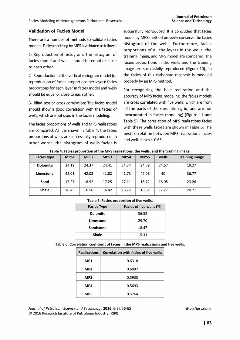
successfully reproduced. It is concluded that facies

model by MPS method properly conserve the facies

histogram of the wells. Furthermore, facies

proportions of all the layers in the wells, the

training image, and MPS model are compared. The

facies proportions in the wells and the training

image are successfully reproduced (Figure 10), so

the facies of this carbonate reservoir is modeled

properly by an MPS method.

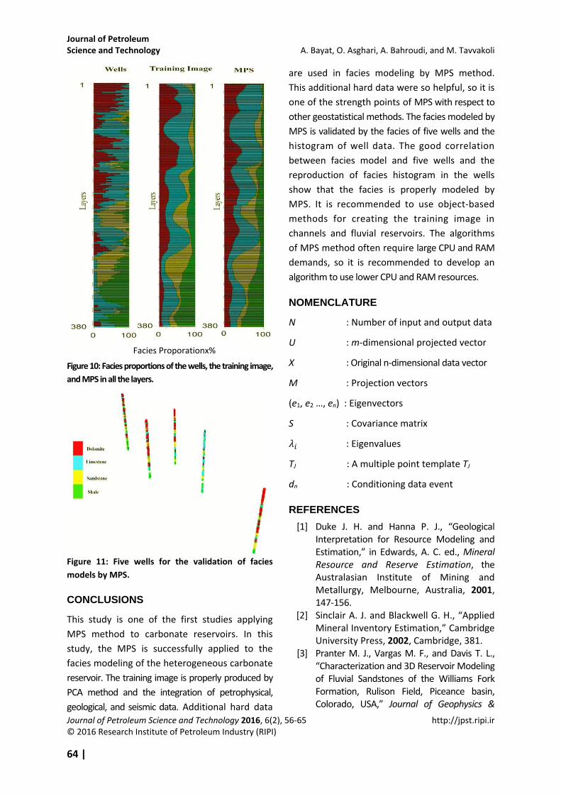
For recognizing the best realization and the

accuracy of MPS facies modeling, the facies models

are cross correlated with five wells, which are from

all the parts of the simulation grid, and are not

incorporated in facies modeling) (Figure 11 and

Table 5). The correlation of MPS realizations facies

with these wells facies are shown in Table 6. The

best correlation between MPS realizations facies

and wells facies is 0.63.

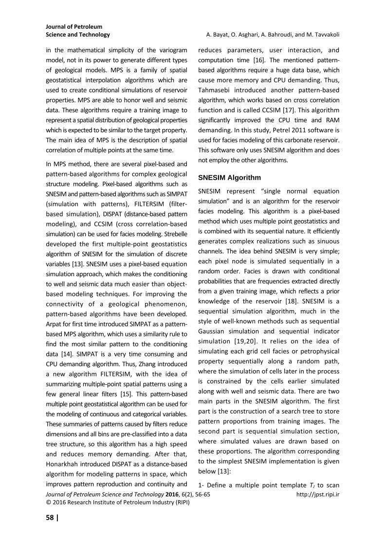
Table 4: Facies proportion of the MPS realizations, the wells, and the training image.

Facies type MPS1 MPS2 MPS3 MPS4 MPS5 wells Training image

Dolomite 24.19 24.37 24.41 24.34 24.59 24.67 19.27

Limestone 42.01 42.05 41.82 41.73 42.08 40 36.77

Sand 17.27 16.92 17.25 17.11 16.72 18.05 23.26

Shale 16.45 16.56 16.42 16.72 16.51 17.27 20.71

Table 5: Facies proportion of five wells.

Facies Type Facies of five wells (%)

Dolomite 36.52

Limestone 29.70

Sandstone 18.47

Shale 15.31

Table 6: Correlation coeficient of facies in the MPS realizations and five wells.

Realizations Correlation with facies of five wells

MP1 0.6318

MP2 0.6097

MP3 0.5935

MP4 0.5693

MP5 0.5764



64 |

Figure 10: Facies proportions of the wells, the training image,

and MPS in all the layers.

Figure 11: Five wells for the validation of facies

models by MPS.

CONCLUSIONS

This study is one of the first studies applying

MPS method to carbonate reservoirs. In this

study, the MPS is successfully applied to the

facies modeling of the heterogeneous carbonate

reservoir. The training image is properly produced by

PCA method and the integration of petrophysical,

geological, and seismic data. Additional hard data

are used in facies modeling by MPS method.

This additional hard data were so helpful, so it is

one of the strength points of MPS with respect to

other geostatistical methods. The facies modeled by

MPS is validated by the facies of five wells and the

histogram of well data. The good correlation

between facies model and five wells and the

reproduction of facies histogram in the wells

show that the facies is properly modeled by

MPS. It is recommended to use object‐based

methods for creating the training image in

channels and fluvial reservoirs. The algorithms

of MPS method often require large CPU and RAM

demands, so it is recommended to develop an

algorithm to use lower CPU and RAM resources.

NOMENCLATURE

N : Number of input and output data

U : m‐dimensional projected vector

X : Original n‐dimensional data vector

M : Projection vectors

(e1, e2 …, en) : Eigenvectors

S : Covariance matrix

: Eigenvalues

TJ : A multiple point template TJ

dn : Conditioning data event

REFERENCES

[1] Duke J. H. and Hanna P. J., “Geological Interpretation for Resource Modeling and Estimation,” in Edwards, A. C. ed., Mineral Resource and Reserve Estimation, the Australasian Institute of Mining and Metallurgy, Melbourne, Australia, 2001, 147‐156.

[2] Sinclair A. J. and Blackwell G. H., “Applied Mineral Inventory Estimation,” Cambridge University Press, 2002, Cambridge, 381.

[3] Pranter M. J., Vargas M. F., and Davis T. L., “Characterization and 3D Reservoir Modeling of Fluvial Sandstones of the Williams Fork Formation, Rulison Field, Piceance basin, Colorado, USA,” Journal of Geophysics &

Facies Proporationx%



| 65

Engineering, 2008, 5, 158‐172. [4] Deutsch C. V., Geostatistical Reservoir

Modeling, Oxford University Press, Oxford, 2002.

[5] Armstrong M., Galli A. G., Le Loc’h G., Geffroy F., et al., Plurigaussian Simulations in Geosciences, Berlin, Springer, 2003, 149.

[6] Guardiano F., and Srivastava M., “Multivariate Geostatistics: beyond Bivariate Moments, in A Soares, Editor, Geostatistics‐Troia, Kluwer Academic Publications,” Quantitative Geology and Geostatistics, 1993, 5, 133–144.

[7] Journel A., “Beyond Covariance: The Advent of Multiple‐point Geostatistics, in Leuangthong, O. and Deutsch, C. Eds.,” 7th International Geostatistics Congress. Banff, Canada, Springer, 2004, 1, 225‐235.

[8] Strebelle S. and Journel A., “Reservoir Modeling Using Multiple Point Statistics,” SPE 71324, 2001.

[9] Liu, Y., “Downscaling Seismic Data into A Geologically Sound Numerical Model,” Ph.D. Thesis, Stanford University, Stanford, 2003.

[10] Jolliffe I. T., Principal Component Analysis, 2nd ed., UK: Springer Series in Statistics, Springer, 2002, 487.

[11] Scheevel J. R. and Payrazyan K., “Principal Component Analysis Applied to 3D Seismic Data for Reservoir Property Estimation,” SPE Presented In The SPE Annual Technical Conference Held in Houston, Texas, USA, 1999.

[12] Caers J., and Zhang T., “Multiple‐point Geostatistics: A Quantitative Vehicle for Integrating Geologic Analogs into Multiple Reservoir Models,” Stanford University, Stanford Center for Reservoir Forecasting, Stanford, 2002, CA 94305‐2220.

[13] Strebelle S., “Sequential Simulation Drawing Structures from Training Images,” Ph.D. Thesis, Stanford University, Stanford, USA, 2000.

[14] Arpat G. B. and Caers J., “A Multiple‐scale, Pattern‐based Approach to Sequential Simulation,” Department of Petroleum Engineering Stanford University, Stanford, USA, 2005, 255‐264.

[15] Zhang T., Filter‐based Training Pattern Classification for Spatial Pattern Simulation, Ph.D. Thesis, Stanford University, USA, 2006.

[16] Honarkhah M., “Stochastic Simulation of Patterns Using Distance‐based Pattern Modeling,” Ph.D. Thesis, Stanford University, USA, 2011.

[17] Tahmasebi P., Hezarkhani A., and Sahimi M., “Multiple Point Geostatistical Modeling Based on the Cross Correlation Functions,” Computational Geosciences, 2012, 16, 779‐797.

[18] Srivastava M., “An Overview of Stochastic Methods for Reservoir Characterization, in Yarus, J., and Chambers, R., Eds., Stochastic Modeling and Geostatistics: Principles, Methods, and Case Studies,” Computer Applications in Geology, AAPG, 1995, 3, 3‐16.

[19] Isaaks, E., “The Application of Monte Carlo Methods to the Analysis of Spatially Correlated Data,” Ph.D. Thesis, Stanford University, Stanford, USA, 1990.

[20] Gomez J. and Srivastava R., “ISIM3D: An ANSI‐C Three Dimensional Multiple Indicator Conditional Simulation,” Computer & Geosciences, 1990, 16, 395–410.

[21] Haldorsen H. and Damsleth E., “Stochastic Modeling,” Journal of Petroleum Technology, 1990, 404‐ 412.

[22] Deutsch C. and Wang L., “Hierarchical Object‐Based Stochastic Modeling of Fluvial Reservoirs, Mathematical Geology,” 1996, 28, 857‐ 880.

[23] Holden L., Hauge R., Skare O., and Skorstad A., “Modeling of Fluvial Reservoirs with Object Models,” Mathematical Geology, 1988, 24, 473‐496.

[24] Viseur S., “Stochastic Boolean Simulation of Fluvial Deposits: A New Approach Combining Accuracy and Efficiency,” Presented at the Annual Technical Conference and Exhibition, Houston, SPE 56688, 1999.

[25] Wen R., Martinius A., Nass A., and Ringrose P., “Three Dimensional Simulation of Small Scale Heterogeneity in Tidal Deposits A Process‐based Stochastic Simulation Method,” International Association for Mathematical Geology, 1998, 399‐400.

Facies Modeling of Heterogeneous Carbonates Reservoirs by ...

Documents

Transcript of Facies Modeling of Heterogeneous Carbonates Reservoirs by ...