Multiple Testing in a Two-Stage Adaptive Design with ...

Multiple Testing in a Two-Stage Adaptive Design with

Combination Tests Controlling FDR

Sanat K. Sarkar, Jingjing Chen and Wenge Guo

March 13, 2012

Sanat K. Sarkar is Cyrus H. K. Curtis Professor, Department of Statistics, Temple

University, Philadelphia, PA 19122 (Email: [email protected]). Jingjing Chen is PhD

candidate, Department of Statistics, Temple University, Philadelphia, PA 19122 (Email:

[email protected]). Wenge Guo is Assistant Professor, Department of Mathematical Sci-

ences, New Jersey Institute of Technology, Newark, NJ 07102 (Email: [email protected]).

The research of Sarkar and Guo were supported by NSF Grants DMS-1006344 and DMS-

1006021 respectively.

ABSTRACT

In many scientific studies requiring simultaneous testing of multiple null hypotheses,

it is often necessary to carry out the multiple testing in two stages to decide which of the

hypotheses can be rejected or accepted at the first stage and which should be followed

up for further testing having combined their p-values from both stages. Unfortunately,

no multiple testing procedure is available yet to perform this task meeting pre-specified

boundaries on the first-stage p-values in terms of the false discovery rate (FDR) and main-

taining a control over the overall FDR at a desired level. We present in this article two

procedures, extending the classical Benjamini-Hochberg (BH) procedure and its adaptive

version incorporating an estimate of the number of true null hypotheses from single-stage

to a two-stage setting. These procedures are theoretically proved to control the overall

FDR when the pairs of first- and second-stage p-values are independent and those corre-

sponding to the null hypotheses are identically distributed as a pair (p1, p2) satisfying the

p-clud property of Brannath, Posch and Bauer (2002, Journal of the American Statistical

Association, 97, 236 -244). We consider two types of combination function, Fisher’s and

Simes’, and present explicit formulas involving these functions towards carrying out the

proposed procedures based on pre-determined critical values or through estimated FDR’s.

Our simulation indicate that the proposed procedures can have significant power improve-

ments over the BH procedure based on the first stage data relative to the improvement

offered by the ideal BH procedure that one would have used had the second stage data

been available for all the hypotheses, at least under independence, and can continue to con-

trol the FDR under some dependence situations. The proposed procedures are illustrated

through a real gene expression data.

Keywords: Combination test; early rejection and acceptance boundaries; false discovery

rate; multiple testing; stepwise multiple testing procedure; two-stage adaptive design.

1 INTRODUCTION

Gene association or expression studies that usually involve a large number of endpoints

(i.e., genetic markers) are often quite expensive. Such studies conducted in a multi-stage

adaptive design setting can be cost effective and efficient, since genes are screened in early

stages and selected genes are further investigated in later stages using additional observa-

tions. Multiplicity in simultaneous testing of hypotheses associated with the endpoints in a

multi-stage adaptive design is an important issue, as in a single stage design. For address-

ing the multiplicity concern, controlling the familywise error rate (FWER), the probability

of at least one type I error among all hypotheses, is a commonly applied concept. However,

these studies are often explorative, so controlling the false discovery rate (FDR), which is

the expected proportion of type I errors among all rejected hypotheses, is more appropri-

ate than controlling the FWER (Weller et al. 1998; Benjamini and Hochberg 1995; and

Storey and Tibshirani 2003). Moreover, with large number of hypotheses typically being

tested in these studies, better power can be achieved in a multiple testing method under

the FDR framework than under the more conservative FWER framework.

Adaptive designs with multiple endpoints have been considered in the literature under

both the FWER and FDR frameworks. Miller et al. (2001) suggested using a two-stage

2

design in gene experiments, and proposed using the Bonferroni method to control the

FWER in testing the hypotheses selected at the first stage, although only the second stage

observations are used for this method. This was later improved by Satagopan and Elston

(2003) by incorporating the first stage data through group sequential schemes in the final

Bonferroni test. Zehetmayer et al. (2005) considered a two-stage adaptive design where

promising hypotheses are selected using a constant rejection threshold for each p-value at

the first stage and an estimation based approach to controlling the FDR asymptotically

(as the number of hypotheses goes to infinity) was taken (Storey 2002; Storey, Taylor and

Siegmund 2004) at the second stage to test the selected hypotheses using more observa-

tions. Zehetmayer et al. (2008) have extended this work from two-stage to multi-stage

adaptive designs under both FDR and FWER frameworks, and provided useful insights

into the power performance of optimized multi-stage adaptive designs with respect to the

number of stages, and into the power difference between optimized integrated design and

optimized pilot design. Posch et al. (2009) showed that a data-dependent sample size in-

crease for all the hypotheses simultaneously in a multi-stage adaptive design has no effect

on the asymptotic (as the number of hypotheses goes to infinity) control of the FDR if

the hypotheses to be rejected are determined only by the test at the final interim analysis,

under all scenarios except the global null hypothesis when all the null hypotheses are true.

Construction of methods with the FWER or FDR control in the setting of a two-stage

adaptive design allowing reduction in the number of tested hypotheses at the interim

analysis has been discussed, as a separate issue from sample size adaptations, in Bauer

and Kieser (1999) and Kieser, Bauer and Lehmacher (1999) , who presented methods with

the FWER control, and in Victor and Hommel (2007) who focused on controlling the FDR

in terms of a generalized global p-values. We revisit this issue in the present paper, but

focusing primarily on the FDR control in a non-asymptotic setting (with the number of

hypothesis not being infinitely large).

Our motivation behind this paper lies in the fact that the theory presented so far (see,

for instance, Victor and Hommel 2007) towards developing an FDR controlling procedure

in the setting of a two-stage adaptive design with combination tests does not seem to be

as simple as one would hope for. Moreover, it does not allow setting boundaries on the

first stage p-values in terms of FDR and operate in a manner that would be a natural

3

extension of standard single-stage FDR controlling methods, like the BH (Benjamini and

Hochberg 1995) or methods related to it, from a single-stage to a two-stage design setting.

So, we consider the following to be our main problem in this paper:

To construct an FDR controlling procedure for simultaneous testing of the

null hypotheses associated with multiple endpoints in the following two-stage

adaptive design setting: The hypotheses are sequentially screened at the first

stage as rejected or accepted based on pre-specified boundaries on their p-

values in terms of the FDR, and those that are left out at the first stage are

again sequentially tested at the second stage having determined their second-

stage p-values based on additional observations and then using the combined

p-values from the two stages through a combination function.

We propose two FDR controlling procedures, one extending the original single-stage

BH procedure, which we call the BH-TSADC Procedure (BH type procedure for two-stage

adaptive design with combination tests), and the other extending an adaptive version of the

single-stage BH procedure incorporating an estimate of the number of true null hypotheses,

which we call the Plug-In BH-TSADC Procedure, from single-stage to a two-stage setting.

Let (p1i, p2i) be the pair of first- and second-stage p-values corresponding to the ith null

hypothesis. We provide a theoretical proof of the FDR control of the proposed procedures

under the assumption that the (p1i, p2i)’s are independent and those corresponding to the

true null hypotheses are identically distributed as (p1, p2) satisfying the p-clud property

(Brannath et al. 2002), and some standard assumption on the combination function.

We consider two special types of combination function, Fisher’s and Simes’, which are

often used in multiple testing applications, and present explicit formulas for probabilities

involving them that would be useful to carry out the proposed procedures at the second

stage either using critical values that can be determined before observing the p-values or

based on estimated FDR’s that can be obtained after observing the p-values.

We carried out extensive simulations to investigate how well our proposed procedures

perform in terms of FDR control and power under independence with respect to the number

of true null hypotheses and the selection of early stopping boundaries. Simulations were

also performed to evaluate whether or not the proposed procedures can continue to control

the FDR under different types of (positive) dependence among the underlying test statistics

4

we consider, such as equal, clumpy and auto-regressive of order one [AR(1)] dependence.

Since potential improvement of the usual FDR controlling BH method based only on the

first-stage data by considering a suitable modification of it in the present two-stage setting,

but still controlling the FDR, is the main motivation behind proposing our methods, it is

natural to measure the power performance of each of our proposed methods against that

of this first-stage BH method. Of course, it seems obvious that our methods will be more

powerful since they utilize more data, and so it won’t be fair to assess this improvement

by merely looking at the power performance and not by measuring it against the power of

the so called best-case-scenario BH method, which is the BH method one would have used

had the second stage data been available for all the endpoints. Also, it is important that

the cost saving our procedure can potentially offer relative to the maximum possible cost

incurred by this ideal BH method be taken into account while assessing this improvement.

Gauging the simulated power improvements offered by our procedures over the first-

stage BH method against that offered by the ideal BH method, we notice that with equal

sample size allocation between the two stages, our procedures based on Fisher’s combi-

nation function are doing much better, at least under independence, than those based

on Simes’ combination function. In terms of power, our procedures based on Fisher’s

combination function is more close to the ideal BH method than to the first-stage BH

method, whereas those based on Simes’ combination function is in the middle between

the first-stage and the ideal BH methods. Between our two procedures, whether they are

based on Fisher’s or Simes’ combination function, the BH-TSADC seems to be the better

choice in terms of controlling the FDR and power improvement over the single-stage BH

procedure when the proportion of true nulls is large. If this proportion is not large, the

Plug-In BH-TSADC procedure is better, but it might lose the FDR control when the p-

values exhibit equal or AR(1) type dependence with a large equal- or auto-correlation. In

terms of cost, our simulations indicate that both our procedures can provide significantly

large savings. With 90% true nulls and half of the total sample size allocated to the first

stage, our procedures can offer 44% saving from the maximum cost incurred by using the

BH method based on the full data from both stages. This proportion gets larger with

increasing proportion of true nulls or decreasing proportion of the sample size allocated to

the first stage.

5

We applied our proposed two-stage procedures to reanalyze the data on multiple

myeloma considered before by Zehetmayer et al. (2008), of course, for a different pur-

pose. The data consist of a set of 12625 gene expression measurements for each of 36

patients with bone lytic lesions and 36 patients in a control group without such lesions.

We considered this data in a two-stage framework, with the first 18 subjects per group

for Stage 1 and the next 18 per group for Stage 2. With some pre-chosen early rejection

and acceptance boundaries, these procedures produce significantly more discoveries than

the first-stage BH procedure relative to the additional discoveries made by the ideal BH

procedure based on the full data from both stages.

The article is organized as follows. We review some basic results on the FDR control

in a single-stage design in Section 2, present our proposed procedures in Section 3, discuss

the results of simulations studies in Section 4, and illustrate the real data application in

Section 5. We make some concluding remarks in Section 6 and give proofs of our main

theorem and propositions in Appendix.

2 CONTROLLING THE FDR IN A SINGLE-STAGE

DESIGN

Suppose that there are m endpoints and the corresponding null hypotheses Hi, i =

1, . . . , m, are to be simultaneously tested based on their respective p-values pi, i = 1, . . . , m,

obtained in a single-stage design. The FDR of a multiple testing method that rejects R

and falsely rejects V null hypotheses is E(FDP), where FDP = V/ max{R, 1} is the false

discovery proportion. Multiple testing is often carried out using a stepwise procedure de-

fined in terms of p(1) ≤ · · · ≤ p(m), the ordered p-values. With H(i) the null hypothesis

corresponding to p(i), a stepup procedure with critical values γ1 ≤ · · · ≤ γm rejects H(i)

for all i ≤ k = max{j : p(j) ≤ γj}, provided the maximum exists; otherwise, it accepts

all null hypotheses. A stepdown procedure, on the other hand, with these same critical

values rejects H(i) for all i ≤ k = max{j : p(i) ≤ γi for all i ≤ j}, provided the maximum

exists, otherwise, accepts all null hypotheses. The following are formulas for the FDR’s

of a stepup or single-step procedure (when the critical values are same in a stepup proce-

dure) and a stepdown procedure in a single-stage design, which can guide us in developing

6

stepwise procedures controlling the FDR in a two-stage design. We will use the notation

FDR1 for the FDR of a procedure in a single-stage design.

Result 1. (Sarkar 2008). Consider a stepup or stepdown method for testing m null

hypotheses based on their p-values pi, i = 1, . . . , m, and critical values γ1 ≤ · · · ≤ γm in a

single-stage design. The FDR of this method is given by

FDR1 ≤∑i∈J0

E

[I(pi ≤ γ

R(−i)m−1(γ2,...,γm)+1

)

R(−i)m−1(γ2, . . . , γm) + 1

],

with the equality holding in the case of stepup method, where I is the indicator function,

J0 is the set of indices of the true null hypotheses, and R(−i)m−1(γ2, . . . , γm) is the number of

rejections in testing the m− 1 null hypotheses other than Hi based on their p-values and

using the same type of stepwise method with the critical values γ2 ≤ · · · ≤ γm.

With pi having the cdf F (u) when Hi is true, the FDR of a stepup or stepdown

method with the thresholds γi, i = 1, . . . , m, under independence of the p-values, satisfies

the following:

FDR1 ≤∑i∈J0

E

(F (γ

R(−i)m−1(γ2,...,γm)+1

)

R(−i)m−1(γ2, . . . , γm) + 1

).

When F is the cdf of U(0, 1) and these thresholds are chosen as γi = iα/m, i = 1, . . . , m,

the FDR equals π0α for the stepup and is less than or equal to π0α for the stepdown

method, where π0 is the proportion of true nulls, and hence the FDR is controlled at α.

This stepup method is the so called BH method (Benjamini and Hochberg, 1995), the most

commonly used FDR controlling procedure in a single-stage deign. The FDR is bounded

above by π0α for the BH as well as its stepdown analog under certain type of positive

dependence condition among the p-values (Benjamini and Yekutieli 2001; Sarkar 2002,

2008).

The idea of improving the FDR control of the BH method by plugging into it a suitable

estimate π0 of π0, that is, by considering the modified p-values π0pi, rather than the original

p-values, in the BH method, was introduced by Benjamini and Hochberg (2000), which was

later brought into the estimation based approach to controlling the FDR by Storey (2002).

7

A number of such plugged-in versions of the BH method with proven and improved FDR

control mostly under independence have been put forward based on different methods

of estimating π0 (for instance, Benjamini, Krieger, and Yekutieli 2006; Blanchard and

Roquain 2009; Gavrilov, Benjamini and Sarkar 2009; Sarkar 2008; and Storey, Taylor and

Siegmund 2004).

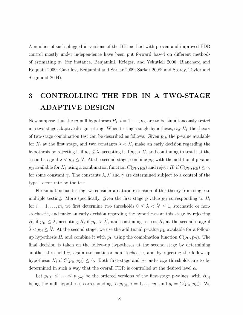
3 CONTROLLING THE FDR IN A TWO-STAGE

ADAPTIVE DESIGN

Now suppose that the m null hypotheses Hi, i = 1, . . . , m, are to be simultaneously tested

in a two-stage adaptive design setting. When testing a single hypothesis, say Hi, the theory

of two-stage combination test can be described as follows: Given p1i, the p-value available

for Hi at the first stage, and two constants λ < λ′, make an early decision regarding the

hypothesis by rejecting it if p1i ≤ λ, accepting it if p1i > λ′, and continuing to test it at the

second stage if λ < p1i ≤ λ′. At the second stage, combine p1i with the additional p-value

p2i available for Hi using a combination function C(p1i, p2i) and reject Hi if C(p1i, p2i) ≤ γ,

for some constant γ. The constants λ, λ′ and γ are determined subject to a control of the

type I error rate by the test.

For simultaneous testing, we consider a natural extension of this theory from single to

multiple testing. More specifically, given the first-stage p-value p1i corresponding to Hi

for i = 1, . . . , m, we first determine two thresholds 0 ≤ λ < λ′ ≤ 1, stochastic or non-

stochastic, and make an early decision regarding the hypotheses at this stage by rejecting

Hi if p1i ≤ λ, accepting Hi if p1i > λ′, and continuing to test Hi at the second stage if

λ < p1i ≤ λ′. At the second stage, we use the additional p-value p2i available for a follow-

up hypothesis Hi and combine it with p1i using the combination function C(p1i, p2i). The

final decision is taken on the follow-up hypotheses at the second stage by determining

another threshold γ, again stochastic or non-stochastic, and by rejecting the follow-up

hypothesis Hi if C(p1i, p2i) ≤ γ. Both first-stage and second-stage thresholds are to be

determined in such a way that the overall FDR is controlled at the desired level α.

Let p1(1) ≤ · · · ≤ p1(m) be the ordered versions of the first-stage p-values, with H(i)

being the null hypotheses corresponding to p1(i), i = 1, . . . , m, and qi = C(p1i, p2i). We

8

describe in the following a general multiple testing procedure based on the above theory,

before proposing our FDR controlling procedures that will be of this type.

A General Stepwise Procedure.

1. For two non-decreasing sequences of constants λ1 ≤ · · · ≤ λm and λ′1 ≤ · · · ≤ λ′m,

with λi < λ′i for all i = 1, . . . , m, and the first-stage p-values p1i, i = 1, . . . , m, define

two thresholds as follows: R1 = max{1 ≤ i ≤ m : p1(j) ≤ λj for all j ≤ i} and

S1 = max{1 ≤ i ≤ m : p1(i) ≤ λ′i}, where 0 ≤ R1 ≤ S1 ≤ m and R1 or S1 equals

zero if the corresponding maximum does not exist. Reject H(i) for all i ≤ R1, accept

H(i) for all i > S1, and continue testing H(i) at the second stage for all i such that

R1 < i ≤ S1.

2. At the second stage, consider q(i), i = 1, . . . , S1 − R1, the ordered versions of the

combined p-values qi = C(p1i, p2i), i = 1, . . . , S1 − R1, for the follow-up null hy-

potheses, and find R2(R1, S1) = max{1 ≤ i ≤ S1 − R1 : q(i) ≤ γR1+i}, given another

non-decreasing sequence of constants γr1+1(r1, s1) ≤ · · · ≤ γs1(r1, s1), for every fixed

r1 < s1. Reject the follow-up null hypothesis H(i) corresponding to q(i) for all i ≤ R2

if this maximum exists, otherwise, reject none of the follow-up null hypotheses.

Remark 1. We should point out that the above two-stage procedure screens out the

null hypotheses at the first stage by accepting those with relatively large p-values through a

stepup procedure and by rejecting those with relatively small p-values through a stepdown

procedure. At the second stage, it applies a stepup procedure to the combined p-values.

Conceptually, one could have used any type of multiple testing procedure to screen out

the null hypotheses at the first stage and to test the follow-up null hypotheses at the

second stage. However, the particular types of stepwise procedure we have chosen at the

two stages provide flexibility in terms of developing a formula for the FDR and eventually

determining explicitly the thresholds we need to control the FDR at the desired level.

Let V1 and V2 denote the total numbers of falsely rejected among all the R1 null

hypotheses rejected at the first stage and the R2 follow-up null hypotheses rejected at the

second stage, respectively, in the above procedure. Then, the overall FDR in this two-stage

9

procedure is given by

FDR12 = E

[V1 + V2

max{R1 + R2, 1}]

.

The following theorem (to be proved in Appendix) will guide us in determining the

first- and second-stage thresholds in the above procedure that will provide a control of

FDR12 at the desired level. This is the procedure that will be one of those we propose in

this article. Before stating the theorem, we need to define the following notations:

• R(−i)1 is defined as R1 in terms of the m− 1 first-stage p-values {p11, . . . , p1m} \ {p1i}

and the sequence of constants λ2 ≤ · · · ≤ λm.

• R(−i)1 and S

(−i)1 are defined as R1 and S1, respectively, in terms of {p11, . . . , p1m}\{p1i}

and the two sequences of constants λ1 ≤ · · · ≤ λm−1 and λ′2 ≤ · · · ≤ λ′m.

• R(−i)2 is defined as R2 with R1 replaced by R

(−i)1 and S1 replaced by S

(−i)1 + 1 and

noting the number of rejected follow-up null hypotheses based on all the combined p-values

except the qi and the critical values other than the first one; that is,

R(−i)2 ≡ R

(−i)2 (R

(−i)1 , S

(−i)1 + 1)

= max{1 ≤ j ≤ S(−i)1 − R

(−i)1 : q

(−i)(j) ≤ γ

R(−i)1 +j+1

(R(−i)1 , S

(−i)1 + 1)},

where q(−i)(j) ’s are the ordered versions of the combined p-values for the follow-up null

hypotheses except the qi.

Theorem 1. The FDR of the above general multiple testing procedure satisfies the

following inequality

FDR12 ≤∑i∈J0

E

[I(p1i ≤ λ

R(−i)1 +1

)

R(−i)1 + 1

]+

∑i∈J0

E

[I(λ

R(−i)1 +1

< p1i ≤ λ′S

(−i)1 +1

, qi ≤ γR

(−i)1 +R

(−i)2 +1,S

(−i)1 +1

)

R(−i)1 + R

(−i)2 + 1

].

The theorem is proved in Appendix.

10

3.1 BH Type Procedures

We are now ready to propose our FDR controlling multiple testing procedures in a two-

stage adaptive design setting with combination function. Before that, let us state some

assumptions we need.

Assumption 1. The combination function C(p1, p2) is non-decreasing in both argu-

ments.

Assumption 2. The pairs (p1i, p2i), i = 1, . . . , m, are independently distributed and

the pairs corresponding the null hypotheses are identically distributed as (p1, p2) with a

joint distribution that satisfies the ‘p-clud’ property (Brannath et al., 2002), that is,

Pr (p1 ≤ u) ≤ u and Pr (p2 ≤ u | p1) ≤ u for all 0 ≤ u ≤ 1.

Let us define the function

H(c; t, t′) =

∫ t′

t

∫ 1

0

I(C(u1, u2) ≤ c)du2du1. 0 < c < 1,

When testing a single hypothesis based on the pair (p1, p2) using t and t′ as the first-

stage acceptance and rejection thresholds, respectively, and c as the second-stage rejection

threshold, H(c; t, t′) is the chance of this hypothesis to be followed up in the second stage

before being rejected when it is null.

Definition 1. (BH-TSADC Procedure).

1. Given the level α at which the overall FDR is to be controlled, three sequences of

constants λi = iλ/m, i = 1, . . . , m, λ′i = iλ′/m, i = 1, . . . , m, for some prefixed

λ < α < λ′, and γr1+1,s1 ≤ · · · ≤ γs1,s1 , satisfying

H(γr1+i,s1 ; λr1 , λ′s1

) =(r1 + i)(α− λ)

m,

i = 1, . . . , s1 − r1, for every fixed 1 ≤ r1 < s1 ≤ m, find R1 = max{1 ≤ i ≤ m :

p1(j) ≤ λj for all j ≤ i} and S1 = max{1 ≤ i ≤ m : p1(i) ≤ λ′i}, with R1 or S1 being

equal to zero if the corresponding maximum does not exist.

11

2. Reject H(i) for i ≤ R1; accept H(i) for i > S1; and continue testing H(i) for R1 <

i ≤ S1 making use of the additional p-values p2i’s available for all such follow-up

hypotheses at the second stage.

3. At the second stage, consider the combined p-values qi = C(p1i, p2i) for the follow-up

null hypotheses. Let q(i), i = 1, . . . , S1 − R1, be their ordered versions. Reject H(i)

[the null hypothesis corresponding to q(i)] for all i ≤ R2(R1, S1) = max{1 ≤ j ≤S1 − R1 : q(j) ≤ γR1+j,S1}, provided this maximum exists, otherwise, reject none of

the follow-up null hypotheses.

Proposition 1. Let π0 be the proportion of true null hypotheses. Then, the FDR

of the BH-TSADC method is less than or equal to π0α, and hence controlled at α, if

Assumptions 1 and 2 hold.

The proposition is proved in Appendix.

The BH-TSADC procedure can be implemented alternatively, and often more conve-

niently, in terms of some FDR estimates at both stages. With R(1)(t) = #{i : p1i ≤ t) and

R(2)(c; t, t′) = #{i : t < p1i ≤ t′, C(p1i, p2i) ≤ c}, let us define

FDR1(t) =

{mt

R(1)(t)if R(1)(t) > 0

0 if R(1)(t) = 0,

and FDR2|1(c; t, t′) =

{mH(c;t,t′)

R(1)(t)+R(2)(c;t,t′) if R(2)(c; t, t′) > 0

0 if R(2)(c; t, t′) = 0,

Then, we have the following:

The BH-TSADC procedure: An alternative definition. Reject H(i) for all i ≤ R1 =

max{1 ≤ k ≤ m : FDR1(p1(j)) ≤ λ for all j ≤ k}; accept H(i) for all i > S1 = max{1 ≤k ≤ m : FDR1(p1(k)) ≤ λ′}; continue to test H(i) at the second stage for all i such that

R1 < i ≤ S1. Reject H(i), the follow-up null hypothesis corresponding to q(i), at the second

stage for all i ≤ R2(R1, S1) = max{1 ≤ k ≤ S1 − R1 : FDR2|1(q(k); R1λ/m, S1λ′/m) ≤

α− λ}.

Remark 2. The BH-TSADC procedure is an extension of the BH procedure, from

12

a method of controlling the FDR in a single-stage design to that in a two-stage adaptive

design with combination tests. When λ = 0 and λ′ = 1, that is, when we have a single-

stage design based on the combined p-values, this method reduces to the usual BH method.

Notice that FDR1(t) is a conservative estimate of the FDR of the single-step test with

the rejection pi ≤ t for each Hi. So, the BH-TSADC procedure screens out those null

hypotheses as being rejected (or accepted) at the first stage the estimated FDR’s at whose

p-values are all less than or equal to λ (or greater than λ′).

Clearly, the BH-TSADC procedure can potentially be improved in terms of having a

tighter control over its FDR at α by plugging a suitable estimate of π0 into it while choosing

the second-stage thresholds, similar to what is done for the BH method in a single-stage

design. As said in Section 2, there are different ways of estimating π0, each of which has

been shown to provide the ultimate control of the FDR, of course when the p-values are

independent, by the resulting plugged-in version of the single-stage BH method (see, e.g.,

Sarkar 2008). However, we will consider the following estimate of π0, which is of the type

considered in Storey, Taylor and Siegmund (2004) and seems natural in the context of the

present adaptive design setting where m−S1 of the null hypotheses are accepted as being

true at the first stage:

π0 =m− S1 + 1

m(1− λ′).

The following theorem gives a modified version of the the BH-TSADC procedure using

this estimate.

Definition 2. (Plug-In BH-TSADC Procedure).

Consider the BH-TSADC procedure with the early decision thresholds R1 and S1

based on the sequences of constants λi = iλ/m, i = 1, . . . , m, and λ′i = iλ′/m,

i = 1, . . . ,m, given 0 ≤ λ < λ′ ≤ 1, and the second-stage critical values γ∗R1+i,S1,

i = 1, . . . , S1 −R1, given by the equations

H(γ∗r1+i,s1; λr1 , λ

′s1

) =(r1 + i)(α− λ)

mπ0

, (1)

for i = 1, . . . , s1 − r1.

13

Proposition 2. The FDR of the Plug-In BH-TSADC method is less than or equal

to α if Assumptions 1 and 2 hold.

A proof of this proposition is given in Appendix.

As in the BH-TSADC procedure, the Plug-In BH-TSADC procedure can also be de-

scribed alternatively using estimated FDR’s at both stages. Let

FDR∗2|1(c; t, t

′) =

{mπ0H(c;t,t′)

R(1)(t)+R(2)(c;t,t′) if R(2)(c; t, t′) > 0

0 if R(2)(c; t, t′) = 0,

Then, we have the following:

The Plug-In BH-TSADC procedure: An alternative definition. At the first stage, decide

the null hypotheses to be rejected, accepted, or continued to be tested at the second stage

based on FDR1, as in (the alternative description of) the BH-TSADC procedure. At

the second stage, reject H(i), the follow-up null hypothesis corresponding to q(i), for all

i ≤ R∗2(R1, S1) = max{1 ≤ k ≤ S1 −R1 : FDR

∗2|1(q(k); R1λ/m, S1λ

′/m) ≤ α− λ}.

3.2 Two Special Combination Functions

We now present explicit formulas of H(c; t, t′) for two special combination functions -

Fisher’s and Simes’ - often used in multiple testing applications.

Fisher’s combination function: C(p1, p2) = p1p2.

HFisher(c; t, t′) =

∫ t′

t

∫ 1

0

I(C(u1, u2) ≤ c) du2du1

=

c ln(

t′t

)if c < t

c− t + c ln(

t′c

)if t ≤ c < t′

t′ − t if c ≥ t′ ,

(2)

for c ∈ (0, 1).

14

Simes’ combination function: C(p1, p2) = min {2 min(p1, p2), max(p1, p2)}.

HSimes(c; t, t′) =

∫ t′

t

∫ 1

0

I(C(u1, u2) ≤ c)du2du1

=

c2(t′ − t) if c ≤ t

c( t′2− t) + c2

2if t < c ≤ min(2t, t′)

c(t′ − t) if t′ < c ≤ 2tc2(1 + t′)− t if 2t < c ≤ t′

c2(1 + 2t′)− c2

2− t if max(2t, t′) ≤ c ≤ 2t′

t′ − t if c ≥ 2t′,

for c ∈ (0, 1).

See also Brannath et al. (2002) for the formula (2). These formulas can be used to

determine the critical values γi’s before observing the combined p-values or to estimate

the FDR after observing the combined p-values at the second stage in the BH-TSADC

and Plug-In BH-TSADC procedures with Fisher’s and Simes’ combination functions. Of

course, for large values of m, it is numerically more challenging to determine the γi’s than

estimating the FDR at the second stage, and so in that case we would recommend using

the alternative versions of these procedures.

Given the p-values from the two stages, Fisher’s combination function allows us to

utilize the evidences from both stages with equal importance towards deciding on the

corresponding null hypothesis. Simes’ combination function, on the other hand, allows us

to make this decision based on the strength of evidence provided by the smaller of the two

p-values relative to the larger one for rejecting the null hypothesis.

4 SIMULATION STUDIES

There are a number of important issues related to our proposed procedures that are worth

investigating. As said in the introduction, modifying the first-stage BH method to make

it more powerful in the present two-stage adaptive design setting, relative to the ideal

BH method that would have been used had the second stage data been collected for

all the hypotheses, of course without losing the ultimate control over the FDR, is an

15

important rationale behind developing our proposed methods. Hence, it is important to

numerically investigate, at least under independence, how well the proposed procedures

control the FDR and how powerful they can potentially be compared to both the first-stage

and ideal BH methods. Since the ultimate control over the FDR has been theoretically

established for our methods only under independence, it would be worthwhile to provide

some insight through simulations into their FDRs under some dependence situations. The

consideration of cost efficiency is as essential as that of improved power performance while

choosing a two-stage multiple testing procedure over its single-stage version, as so it is

also important to provide numerical evidence of how much cost savings our procedures

can offer relative to the maximum possible cost incurred by using the ideal BH method.

We conducted our simulation studies addressing these issues. More details about these

studies and conclusions derived from them are given in the following subsections.

4.1 FDR and Power Under Independence

To investigate how well our procedures perform relative to the first-stage and full-data BH

methods under independence, we (i) generated two independent sets of m uncorrelated

random variables Zi ∼ N(µi, 1), i = 1, . . . , m, one for Stage 1 and the other for Stage

2, having set mπ0 of these µi’s at zero and the rest at 2; (ii) tested Hi : µi = 0 against

Ki : µi > 0, simultaneously for i = 1, . . . , m, by applying each of the following procedures

at α = 0.05 to the generated data: The (alternative versions of) BH-TSADC and Plug-In

BH-TSADC procedures with both Fisher’s and Simes’ combination functions, the first-

stage BH method, and the BH method based on combining the data from two stages

(which we call the full-data BH method); and (iii) noted the false discovery proportion

and the proportion of false nulls that are rejected. We repeated steps (i)-(iii) 1000 times

and averaged out the above proportions over these 1000 runs to obtain the final simulated

values of FDR and average power (the expected proportion of false nulls that are rejected)

for each of these procedures.

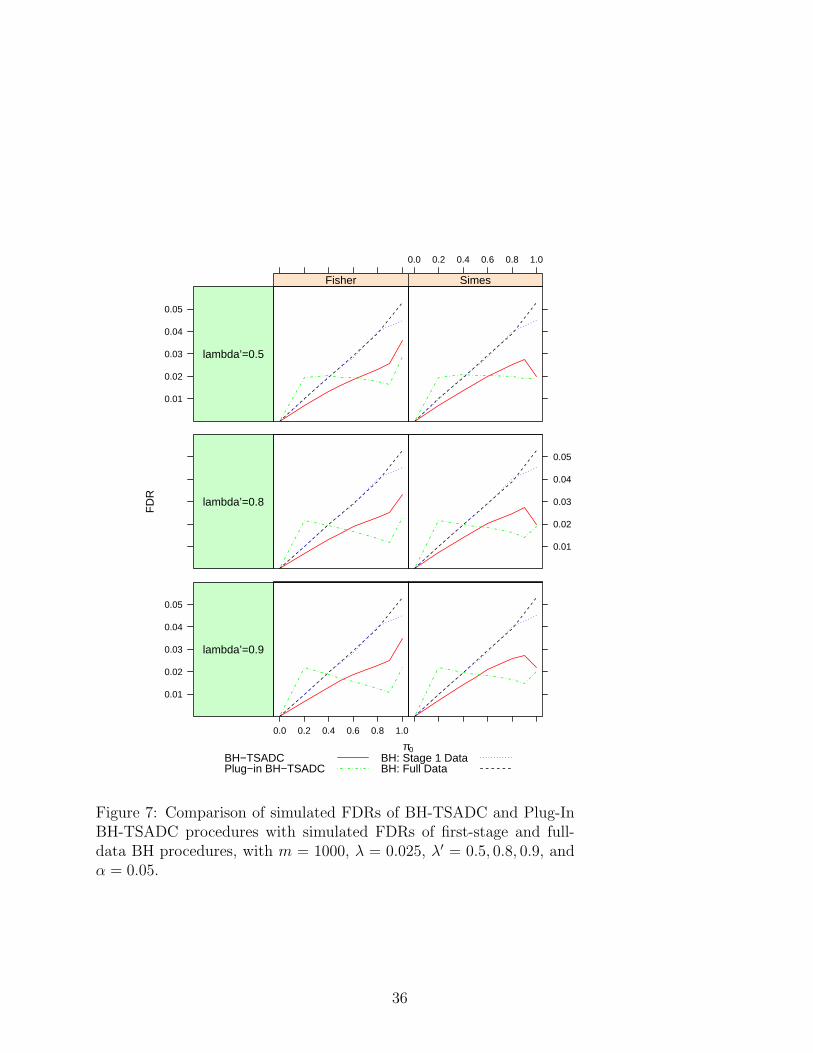
The simulated FDRs and average powers of these procedures for different values of

π0 and selections of early stopping boundaries have been graphically displayed in Figures

1-8. Figures 1 and 3 compare the BH-TSADC and Plug-In BH-TSADC procedures based

on both Fisher’s and Simes combination functions with the first-stage and full-data BH

16

procedures for m = 100 (Figure 1) and 1000 (Figure 3), the early rejection boundary

λ = 0.005, 0.010, or 0.025, and the early acceptance boundary λ′ = 0.5; whereas, Figures

2 and 4 do the same in terms of the average power. Figures 5 to 8 are reproductions of

Figures 1 to 4, respectively, with different early rejection boundary λ = 0.025 and early

acceptance boundary λ′ = 0.5, 0.8, or 0.9.

To examine the performance of our proposed procedures in a more complicated genetic

mode, we explored a model with equally spaced exponentially decreasing effect sizes at

1.5× (22, 21, 20.5, 20). The simulation results can be found in the supplementary materials

of this article. These results show that our procedures are more powerful in presence of

such exponentially decreasing effect sizes than with a constant effect size for the alternative

hypotheses.

4.2 FDR Under Dependence

We considered three different scenarios for dependent p-values in our simulation study

to investigate the FDR control of our procedures under dependence. In particular, we

generated two independent sets of m = 100 correlated normal random variables Zi ∼N(µi, 1), i = 1, . . . , m, one for Stage 1 and the other for Stage 2, with mπ0 of the µi’s

being equal to 0 and the rest being equal to 2, and a correlation matrix exhibiting one

of three different types of dependence - equal, clumpy and AR(1) dependence. In other

words, the Zi’s were assumed to have a common, non-negative correlation ρ in case of

equal dependence, were broken up into ten independent groups with 10 of the Zi’s within

each group having a common, non-negative correlation ρ in case of clumpy dependence,

and were assumed to have correlations ρij = Cor(Zi, Zj) of the form ρij = ρ|i−j| for all

i 6= j = 1, . . . , m, and some non-negative ρ in case of AR(1) dependence. We then applied

the (alternative versions of) the BH-TSADC and Plug-In BH-TSADC procedures at level

α = 0.05 with both Fisher’s and Simes combination functions, λ = 0.025, and λ′ = 0.5 to

these data sets. These two steps were repeated 1000 times before obtaining the simulated

FDR’s and average powers for these procedures, as in our study related to the independence

case.

Figures 9-11 graphically display the simulated FDRs of these procedures for different

values of π0 and types of dependent p-values considered.

17

Table 1: Simulated values of the expected proportion of cost saving (with λ = 0.025 andλ′ = 0.5)

m = 100 m = 1000 m = 5000π0 = 0.5 π0 = 0.9 π0 = 0.5 π0 = 0.9 π0 = 0.5 π0 = 0.9

f = 0.25 0.4321 0.5653 0.4337 0.5716 0.4336 0.5723f = 0.50 0.2405 0.4325 0.2442 0.4401 0.2442 0.4407f = 0.75 0.1075 0.2300 0.1082 0.2319 0.1090 0.2320

4.3 Cost Saving

Let’s consider determining the cost saving in the context of a genome-wide association

study. Because of high cost of genotyping hundreds of thousands of markers on thousands

of subjects, such genotyping is often carried out in a two-stage format. A proportion of

the available samples are genotyped on a large number of markers in the first stage, and a

small proportion of these markers are selected and then followed up by genotyping them

on the remaining samples in the second stage.

Suppose that c is the unit cost of genotyping one marker for each patient, n is the total

number of patients assigned across stages 1 and 2, and m is the total number of markers

for each patient. Then, if we had to apply the full-data BH method, the total cost of

genotyping for all these patients would be n×m× c. Whereas, if we apply our proposed

methods with a fraction f of the n patients assigned to stage 1, then the expected total

cost would be f × n ×m × c + (1 − f) × n × [m − E(S(f))] × c, where S(f) is the total

number of rejected and accepted hypotheses in the first stage. Thus, for our proposed

methods, the expected proportion of saving from the maximum possible cost of using the

full-data BH method is

(1− f)× n× E(S(f))× c

m× n× c=

(1− f)E(S(f))

m.

Table 1 presents the simulated values of this expected proportion of cost saving for our

proposed two-stage methods in multiple testing of m (= 100, 1000, or 5000) independent

normal means in the present two-stage setting with a fraction f (= 0.25, 0.50, 0.75, or 1.00)

of the total number of patients being allocated to the first stage.

18

4.4 Conclusions

Our simulations in Sections 4.1 and 4.2 mimic the scenarios with equal allocation of sample

size between the two stages. So, if we measure the performance of a two-stage procedure by

how much power improvement it can offer over the first-stage BH method relative to that

offered by the ideal, full-data BH method, then our proposed two-stage FDR controlling

procedures with Fisher’s combination function are seen from Figures 1-8 to do much better

under such equal allocation, at least when the p-values are independent both across the

hypotheses and stages, than those based on Simes’ combination function. Of course, our

procedures based on Simes’ combination function are doing reasonably well in terms of

this measure of relative power improvement. It’s performance is roughly between those

of the first-stage and the full-data BH methods. Between our two proposed procedures,

whether it’s based on Fisher’s or Simes’ combination function, the BH-TSADC appears

to be the better choice when π0 is large, like more than 50%, which is often the case in

practice. It controls the FDR not only under independence, which is theoretically known,

but also the FDR control seems to be maintained even under different types of positive

dependence, as seen from Figures 9-11. If, however, π0 is not large, the Plug-In BH-

TSADC procedure provides a better control of the FDR, although it might lose the FDR

control when the statistics generating the p-values exhibit equal or AR(1) type dependence

with a moderately large equal- or auto-correlation. Also seen from Figures 1-8, there is no

appreciable difference in the power performances of the proposed procedures over different

choices of the early stopping boundaries. From Table 1, we notice that our two-stage

methods can provide large cost savings. For instance, with 90% true nulls and half of the

total sample size allocated to the first stage, our procedures can offer 44% saving from

the maximum cost of using the ideal, full-data BH method. This proportion gets larger

with increasing proportion of true nulls or decreasing proportion of the total sample size

allocated to the first stage.

5 A REAL DATA APPLICATION

To illustrate how the proposed procedures can be implemented in practice, we reanalyzed

a dataset taken from an experiment by Tian et al. (2003) and post-processed by Jeffery et

19

al. (2006). Zehetmayer et al. (2008) considered this data for a different purpose. In this

data set, multiple myeloma samples were generated with Affymetrix Human U95A chips,

each consisting 12, 625 probe sets. The samples were split into two groups based on the

presence or absence of focal lesions of bone.

The original dataset contains gene expression measurements of 36 patients without and

137 patients with bone lytic lesions, However, for the illustration purpose, we used the gene

expression measurements of 36 patients with bone lytic lesions and a control group of the

same sample size without such lesions. We considered this data in a two-stage framework,

with the first 18 subjects per group for Stage 1 and the next 18 subjects per group for

Stage 2. We prefixed the Stage 1 early rejection boundary λ at 0.005, 0.010, or 0.015, and

the early acceptance boundary λ′ at 0.5, 0.8 or 0.9, and applied the proposed (alternatives

versions of) BH-TSADC and plug-in BH-TSADC procedures at the FDR level of 0.025.

In particular, we considered all m = 12, 625 probe set gene expression measurements for

the first stage data of 36 patients (18 patients per group) and the full data of 72 patients (36

patients per group) across two stages, and analyzed them based on a stepdown procedure

with the critical values λi = iλ/m, i = 1, . . . , m, and a stepup procedure with the critical

values λ′i = iλ′/m, i = 1, . . . , m, using the corresponding p-values generated from one-

sided t-tests applied to the first-stage data. We noted the probe sets that were rejected

by the stepdown procedure and those that were accepted by the stepup procedure. With

these numbers being r1 and m− s1, respectively, we took the probe sets that were neither

rejected by the stepdown procedure nor accepted by the stepup procedure, that is, the

probe sets with the first-stage p-values more than r1λ/m but less than or equal to s1λ′/m,

for further analysis using estimated FDR based on their first-stage and second-stage p-

values combined through Fisher’s and Simes’ combination functions as described in the

alternative versions of the BH-TSADC and plug-in BH-TSADC procedures.

The results of this analysis are reported in Table 2. As seen from this table, the BH-

TSADC with Fisher’s combination function is doing the best. For instance, with λ = 0.005

and λ′ = 0.9, the proportion of additional discoveries it makes over the first-stage BH

method is 104/125 = 83.2% of such additional discoveries that the ideal, full-data BH

method could make; whereas, these percentages are 52/125 = 41.6%, 32/125 = 25.6%,

and 16/125 = 12.8% for the BH-TSADC with Simes’ combination function, the Plug-

20

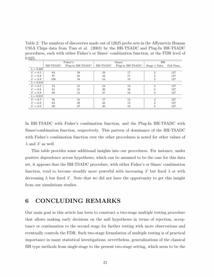
Table 2: The numbers of discoveries made out of 12625 probe sets in the Affymetrix HumanU95A Chips data from Tian et al. (2003) by the BH-TSADC and Plug-In BH-TSADCprocedures, each with either Fisher’s or Simes’ combination function, at the FDR level of0.025.

Fisher’s Simes’ BHBH-TSADC Plug-in BH-TSADC BH-TSADC Plug-in BH-TSADC Stage 1 Data Full Data

λ = 0.005λ′ = 0.5 84 58 33 17 2 127λ′ = 0.8 97 35 42 17 2 127λ′ = 0.9 106 34 54 18 2 127λ = 0.010λ′ = 0.5 74 41 24 13 2 127λ′ = 0.8 81 31 30 16 2 127λ′ = 0.9 90 31 37 18 2 127λ = 0.015λ′ = 0.5 56 31 17 12 2 127λ′ = 0.8 63 29 23 15 2 127λ′ = 0.9 69 27 30 18 2 127

In BH-TSADC with Fisher’s combination function, and the Plug-In BH-TSADC with

Simes’combination function, respectively. This pattern of dominance of the BH-TSADC

with Fisher’s combination function over the other procedures is noted for other values of

λ and λ′ as well.

This table provides some additional insights into our procedures. For instance, under

positive dependence across hypotheses, which can be assumed to be the case for this data

set, it appears that the BH-TSADC procedure, with either Fisher’s or Simes’ combination

function, tend to become steadily more powerful with increasing λ′ but fixed λ or with

decreasing λ but fixed λ′. Note that we did not have the opportunity to get this insight

from our simulations studies.

6 CONCLUDING REMARKS

Our main goal in this article has been to construct a two-stage multiple testing procedure

that allows making early decisions on the null hypotheses in terms of rejection, accep-

tance or continuation to the second stage for further testing with more observations and

eventually controls the FDR. Such two-stage formulation of multiple testing is of practical

importance in many statistical investigations; nevertheless, generalizations of the classical

BH type methods from single-stage to the present two-stage setting, which seem to be the

21

most natural procedures to consider, have not been put forward until the present work. We

have been able to construct two such generalizations with proven FDR control under in-

dependence. We have provided simulation results showing their meaningful improvements

over the first-stage BH method relative to that offered by the ideal BH method in terms

of both power and cost saving under independence, and given an example of their utilities

in practice. We also have presented numerical evidence that the proposed procedures can

maintain a control over the FDR even under some dependence situations.

It is important to emphasize that the theory behind the developments of our proposed

two-stage FDR controlling methods has been driven by the idea of setting the early decision

boundaries λ < λ′ on the (estimated) FDR at the first-stage p-values, rather than on

these p-values themselves. In other words, we flag those null hypotheses for rejection (or

acceptance) at the first stage at whose p-values the estimated FDR’s are all less than or

equal to λ (or greater than λ′) before proceeding to the second stage; see Remark 2. This,

we would argue, is often practical and meaningful when we are testing multiple hypotheses

in two-stages in an FDR framework.

Brannath et al. (2002) have defined a global p-value p(p1, p2) for testing a single

hypothesis in a two-stage adaptive design with combination function C(p1, p2). With the

boundaries λ < λ′ set on each p1i, the global p-value for each Hi is defined by

pi ≡ p(p1i, p2i) =

{p1i if p1i ≤ λ or p1i > λ′

λ + H(C(p1i, p2i); λ, λ′) if λ < p1i ≤ λ′ .

They have shown that each pi is stochastically larger than or equal to U(0, 1) when (p1i, p2i)

satisfies the p-clud property, and the equality holds when p1i and p2i are independently

distributed as U(0, 1). So, one may consider the BH method based on the pi’s. This would

control the overall FDR under the assumptions considered in the paper, maybe under

some positive dependence conditions as well. However, it does not set the early decision

boundaries on the FDR.

We proposed our FDR controlling procedures in this paper considering a non-asymptotic

setting. However, one may consider developing procedures that would asymptotically con-

trol the FDR by taking the following approach towards finding the first- and second-stage

thresholds subject to the early boundaries λ < λ′ and the final boundary α on the FDR.

22

Given two constants t < t′, make an early decision regarding Hi by rejecting it if p1i ≤ t,

accepting it if p1i > t′, and continuing to test it at the second stage if t < p1i ≤ t′. At the

second stage, reject Hi if C(p1i, p2i) ≤ c. Storey’s (2002) estimate of the first-stage FDR

is given by

FDR∗1(t) =

{mπ0t

R(1)(t)if R(1)(t) > 0

0 if R(1)(t) = 0 ,

for some estimate π0 of π0. Similarly, the overall FDR can be estimated as follows:

FDR∗12(c, t, t

′) =

{mπ0[t+H(c;t,t′)]

R(1)(t)+R(2)(c;t,t′) if R(1)(t) + R(2)(c; t, t′) > 0

0 if R(1)(t) + R(2)(c; t, t′) = 0

Let

tλ = sup{t : FDR1(t′) ≤ λ for all t′ ≤ t},

tλ′ = inf{t : FDR1(t′) > λ′ for all t′ > t},

and cα(λ, λ′) = sup{c : FDR12(c, tλ, tλ′) ≤ α}.

Then, reject Hi if p1i ≤ tλ or if tλ < p1i ≤ tλ′ and C(p1i, p2i) ≤ cα(λ, λ′). This may control

the overall FDR asymptotically under the weak dependence condition and the consistency

property of π0 (as in Storey, Taylor and Siegmund 2004).

There are a number of other important issues related to the present problem which we

have not touched in this paper but hope to address in different communications. There

are other combination functions, such as Fisher’s weighted product (Fisher 1932) and

weighted inverse normal (Mosteller and Bush 1954); their performances would be worth

investigating. Consideration of the conditional error function (Proschan and Hunsberger

1995) while defining a two-stage design before constructing FDR controlling methods is

another important issue. Now that we know how to test multiple hypotheses in a two-stage

design subject to first-stage boundaries on and the overall control of the FDR, we should

be able to address issues relate to sample size determinations.

23

7 Appendix

Proof of Theorem 1.

FDR12 = E

[V1 + V2

max{R1 + R2, 1}]≤ E

[V1

max{R1, 1}]

+ E

[V2

max{R1 + R2, 1}]

.

Now,

E

[V1

max{R1, 1}]

=∑i∈J0

E

[I(p1i ≤ λR1)

max{R1, 1}]

=∑i∈J0

E

[I(p1i ≤ λR1)

max{R1, 1}]

≤∑i∈J0

E

[I(p1i ≤ λ

R(−i)1 +1

)

R(−i)1 + 1

];

(as shown in Sarkar, 2008; see also Result 1). And,

E

[V2

max{R1 + R2, 1}]

=∑i∈J0

E

[I(λR1+1 < p1i ≤ λ′S1

, qi ≤ γR1+R2,S1 , S1 > R1, R2 > 0)

R1 + R2

]. (3)

Writing R2 more explicitly in terms of R1 and S1, we see that the expression in (3) is equal

24

to

∑i∈J0

m∑s1=1

s1−1∑r1=0

s1−r1∑r2=1

E

[I(λr1+1 < p1i ≤ λ′s1

, qi ≤ γr1+r2,s1 , R1 = r1, S1 = s1, R2(r1, s1) = r2)

r1 + r2

]

=∑i∈J0

m∑s1=1

s1−1∑r1=0

s1−r1∑r2=1

E

[I(λr1+1 < p1i ≤ λ′s1

, qi ≤ γr1+r2,s1R(−i)1 = r1, S

(−i)1 = s1 − 1, R

(−i)2 (r1, s1) = r2 − 1)

r1 + r2

]

=∑i∈J0

m−1∑s1=0

s1∑r1=0

s1−r1∑r2=0

E

[I(λr1+1 < p1i ≤ λ′s1+1, qi ≤ γr1+r2+1,s1+1, R

(−i)1 = r1, S

(−i)1 = s1, R

(−i)2 (r1, s1 + 1) = r2)

r1 + r2 + 1

]

=∑i∈J0

E

[I(λ

R(−i)1 +1

< p1i ≤ λ′S

(−i)1 +1

, qi ≤ γR

(−i)1 +R

(−i)2 +1,S

(−i)1 +1

)

R(−i)1 + R

(−i)2 + 1

].

Thus, the theorem is proved.

Proof of proposition 1.

FDR12 ≤∑i∈J0

E

[PrH(p1 ≤ λ

R(−i)1 +1

)

R(−i)1 + 1

]+

∑i∈J0

E

[PrH(λ

R(−i)1 +1

< p1 ≤ λ′S

(−i)1 +1

, C(p1, p2) ≤ γR

(−i)1 +R

(−i)2 +1,S

(−i)1 +1

)

R(−i)1 + R

(−i)2 + 1

]

≤∑i∈J0

E

[λ

R(−i)1 +1

R(−i)1 + 1

]+

∑i∈J0

E

[Pr(λ

R(−i)1 +1

< u1 ≤ λ′S

(−i)1 +1

, C(u1, u2) ≤ γR

(−i)1 +R

(−i)2 +1,S

(−i)1 +1

)

R(−i)1 + R

(−i)2 + 1

].

(4)

The first sum in (4) is less than or equal to π0λ, since λR

(−i)1 +1

= [R(−i)1 + 1]λ/m, and the

second sum is less than or equal to π0(α − λ), since the probability in the numerator in

25

this sum is equal to

H(γR1

(−i)+R

(−i)2 +1,S

(−i)1 +1

; λR1

(−i)+1

, λ′S

(−i)1 +1

)

=

[R

(−i)1 + 1 + R

(−i)2

](α− λ)

m.

Thus, the proposition is proved.

Proof of Proposition 2. This can be proved as in Proposition 1. More specifically,

first note that the FDR here, which we call the FDR∗12, satisfies the following:

FDR∗12 ≤

∑i∈J0

E

[I(p1i ≤ λ

R(−i)1 +1

)

R(−i)1 + 1

]+

∑i∈J0

E

[I(λ

R(−i)1 +1

≤ p1i ≤ λ′S

(−i)1 +1

, qi ≤ γ∗R

(−i)1 +R

∗(−i)2 +1,S

(−i)1 +1

)

R(−i)1 + R

∗(−i)2 + 1

],

(5)

where

R∗(−i)2 ≡ R

∗(−i)2 (R

(−i)1 , S

(−i)1 + 1)

= max{1 ≤ j ≤ S(−i)1 − R

(−i)1 : q

(−i)(j) ≤ γ∗

R(−i)1 +j+1,S

(−i)1 +1

},

with q(−i)(j) being the ordered versions of the combined p-values except the qi. As in Propo-

sition 1, the first sum in (5) is less than or equal to π0λ. Before working with the second

sum, first note that the γ∗ satisfying Eqn. (1), that is, the following equation

H(γ∗r1+i,s1; λr1 , λ

′s1

) =(r1 + i)(α− λ)(1− λ′)

m− S1 + 1,

is less than or equal to the γ∗∗ satisfying

H(γ∗∗r1+i,s1; λr1 , λ

′s1

) =(r1 + i)(α− λ)(1− λ′)

m− S(−j)1

,

26

for any fixed j = 1, . . . , m. So, the second sum in (5) is less than or equal to

∑i∈J0

E

[I(λ

R(−i)1 +1

≤ p1i ≤ λ′S

(−i)1 +1

, qi ≤ γ∗∗R

(−i)1 +R

∗(−i)2 +1,S

(−i)1 +1

)

R(−i)1 + R

∗(−i)2 + 1

]

=∑i∈J0

E

[H(γ∗∗

R(−i)1 +R

∗(−i)2 +1,S

(−i)1 +1

; λR

(−i)1 +1

, λ′S

(−i)1 +1

)

R(−i)1 + R

∗(−i)2 + 1

]

= (α− λ)∑i∈J0

E

[1− λ′

m− S(−i)1

]≤ α− λ,

since∑

i∈J0E

[1−λ′

m−S(−i)1

]≤ 1; see, for instance, Sarkar (2008, p. 151). Hence, FDR∗

12 ≤π0λ + α− λ ≤ α, which proves the proposition.

References

[1] Bauer, P., and Kieser, M. (1999), “Combining Different Phases in the Development of

Medical Treatments within a Single Trial,” Statistics in Medicine, 18, 1833-1848.

[2] Benjamini, Y., and Hochberg, Y. (1995), “Controlling the False Discovery Rate: A

Practical and Powerful Approach to Multiple Testing,” Journal of the Royal Statistical

Society, Series B, 57, 289-300.

[3] Benjamini, Y., and Hochberg, Y. (2000), “On the Adaptive Control of the False Dis-

covery Rate in Multiple Testing with Independent Statistics,” Journal of Educational

and Behavioral Statistics, 25, 6083.

[4] Benjamini, Y., Krieger, A., and Yekutieli, D. (2006), “Adaptive Linear Step-up False

Discovery Rate Controlling Procedures,” Biometrika, 93(3), 491-507.

[5] Benjamini, Y., and Yekutieli, D. (2001), “The Control of the False Discovery Rate in

Multiple Testing under Dependency. Annals of Statistics, 29, 1165-1188.

[6] Blanchard, G., and Roquain, E. (2009), “Adaptive FDR Control under Independence

and Dependence,” Journal of Machine Learning Research, 10, 2837-2871.

27

[7] Brannath, W., Posch, M., and Bauer, P. (2002), “Recursive combination tests,” Journal

of the American Statistical Association, 97 (457), 236-244.

[8] Fisher, R.A. (1932), Statistical Methods for Research Workers(4th edition), Lon-

don:Oliver and Boyd.

[9] Gavrilov, Y., Benjamini, Y., and Sarkar, S.K. (2009), “An Adaptive Step-down Pro-

cedure with Proven FDR Control under Independence,” Annals of Statistics, 37(2),

619-629.

[10] Jeffery, I., Higgins, D., and Culhance, A. (2006), “Comparison and Evaluation of

Methods for Generating Differentiall Expressed Genes Lists from Microarray Data,”

BMC Bioinformatics, 7, 359-375.

[11] Kieser, M., Bauer, P., and Lehmacher., W. (1999), “Inference on Multiple Endpoints

in Clinical Trials with Adaptive Interim Analyses,” Biometrical Journal, 41, 261-277.

[12] Miller, R., Galecki, A., and Shmookler-Reis, R. (2001), “Interpretation, Design, and

Analysis of Gene Array Expression Experiments,” J Gerontol A-Biol, 56, B52-B57.

[13] Mosteller, F., and Bush, R. (1954), “Selected Quantitative Techniques,” Handbook of

Social Psychology, 1.

[14] Posch, M., Zehetmayer, S., and Bauer, P. (2009), “Hunting for Significance with

the False Discovery Rate,” Journal of the American Statistical Association, 104(486),

832-840.

[15] Proschan, M., and Hunsberger, S. (1995), “Designed Extension of Studies Based on

Conditional Power,” Biometrics, 51, 1315-1324.

[16] Santagopan, J., and Elston, R. (2003), “Optimal Two-stage Genotyping in

Population-Based Association Studies,” Genetic Epidemiology, 25, 149-157.

[17] Sarkar, S. K. (2002), “Some Results on False Discovery Rate in Stepwise Multiple

Testing Procedures,” Annals of Statistics, 30, 239-257.

[18] Sarkar, S. K. (2008), “On Methods Controlling the False Discovery Rate,” Sankhya:

Series A, 70, 135-168.

28

[19] Storey, J. (2002), “A Direct Approach to False Discovery Rates,” Journal of the Royal

Statistical Society: Series B, 64, 479-498.

[20] Storey, J., Taylor, J., and Siegmund, D. (2004), “Strong Control, Conservative Point

Estimation and Simultaneous Conservative Consistency of False Discovery Rates: a

Unified Approach,” Journal of the Royal Statistical Society: Series B, 66, 187-205.

[21] Storey, J., and Tibshirani, R. (2003), “Statistical Significance in Genomewide Stud-

ies,” Proceedings of the National Academy of Science USA, 100, 9440-9445.

[22] Tian, E., Zhan, F., Walker, R., Rasmussen, E., Ma, Y., and Barlogie, B. (2003), “The

Role of the WNT-signaling Antagonist DKKI in the Development of Osteolytic Lesions

in Multple Myeloma,” New England Journal of Medicine, 349, 2438-2494.

[23] Victor, A., and Hommel, G. (2007), “Combining Adaptive Design with Control of

the False Discovery Rate - a Generalized Definition for a Global P-value,” Biometrical

Journal, 49, 94-106.

[24] Weller, J., Song, J., Heyen, D., Lewin, H., and Ron, M. (1998), “A New Approach

to the Problem of Multiple Comparisons in the Genetic Dissection of Complex Traits,”

Genetics, 150, 1699-1706.

[25] Zehetmayer, S., Bauer, P., and Posch, M. (2005), “Two-stage Designs for Experiments

with a Large Number of Hypotheses,” Bioinformatics, 21, 3771-3777.

[26] Zehetmayer, S., Bauer, P., and Posch, M. (2008), “Optimized Multi-stage Designs

Controlling the False Discovery or the Family-wise Error Rate,” Statistics in Medicine,

27, 4145-4160.

29

π0

FD

R

0.01

0.02

0.03

0.04

0.05

Fisher

lambda=0.005

0.0 0.2 0.4 0.6 0.8 1.0

Simes

lambda=0.005

Fisher

lambda=0.010

0.01

0.02

0.03

0.04

0.05

Simes

lambda=0.010

0.01

0.02

0.03

0.04

0.05

0.0 0.2 0.4 0.6 0.8 1.0

Fisher

lambda=0.025

Simes

lambda=0.025

BH−TSADCPlug−in BH−TSADC

BH: Stage 1 DataBH: Full Data

Figure 1: Comparison of simulated FDRs of BH-TSADC and Plug-InBH-TSADC procedures with simulated FDRs of first-stage and full-data BH procedures, with m = 100, λ = 0.005, 0.010,and 0.025, λ′ =0.5, and α = 0.05.

30

π0

pow

er

0.2

0.4

0.6

0.8

1.0Fisher

lambda=0.005

0.0 0.2 0.4 0.6 0.8 1.0

Simes

lambda=0.005

Fisher

lambda=0.010

0.2

0.4

0.6

0.8

1.0Simes

lambda=0.010

0.2

0.4

0.6

0.8

1.0

0.0 0.2 0.4 0.6 0.8 1.0

Fisher

lambda=0.025

Simes

lambda=0.025



Figure 2: Comparison of simulated average powers of BH-TSADC andPlug-In BH-TSADC procedures with simulated average powers of first-stage and full-data BH procedures, with m = 100, λ = 0.005, 0.010,and 0.025, λ′ = 0.5, and α = 0.05.

31

π0

FD

R

0.01

0.02

0.03

0.04

0.05

Fisher

lambda=0.005

0.0 0.2 0.4 0.6 0.8 1.0

Simes

lambda=0.005

Fisher

lambda=0.010

0.01

0.02

0.03

0.04

0.05

Simes

lambda=0.010

0.01

0.02

0.03

0.04

0.05

0.0 0.2 0.4 0.6 0.8 1.0

Fisher

lambda=0.025

Simes

lambda=0.025



Figure 3: Comparison of simulated FDRs of BH-TSADC and Plug-InBH-TSADC procedures with simulated FDRs of first-stage and full-data BH procedures, with m = 1000, λ = 0.005, 0.010, 0.025, λ′ = 0.5,and α = 0.05.

32

π0

pow

er

0.2

0.4

0.6

0.8

1.0Fisher

lambda=0.005

0.0 0.2 0.4 0.6 0.8 1.0

Simes

lambda=0.005

Fisher

lambda=0.010

0.2

0.4

0.6

0.8

1.0Simes

lambda=0.010

0.2

0.4

0.6

0.8

1.0

0.0 0.2 0.4 0.6 0.8 1.0

Fisher

lambda=0.025

Simes

lambda=0.025



Figure 4: Comparison of simulated average powers of BH-TSADCand Plug-In BH-TSADC procedures with simulated average powersof first-stage and full-data BH procedures, with m = 1000, λ =0.005, 0.010, 0.025, λ′ = 0.5, and α = 0.05.

33

π0

FD

R

0.01

0.02

0.03

0.04

0.05

Fisher

lambda’=0.5

0.0 0.2 0.4 0.6 0.8 1.0

Simes

lambda’=0.5

Fisher

lambda’=0.8

0.01

0.02

0.03

0.04

0.05

Simes

lambda’=0.8

0.01

0.02

0.03

0.04

0.05

0.0 0.2 0.4 0.6 0.8 1.0

Fisher

lambda’=0.9

Simes

lambda’=0.9



Figure 5: Comparison of simulated FDRs of BH-TSADC and Plug-InBH-TSADC procedures with simulated FDRs of first-stage and full-data BH procedures, with m = 100, λ = 0.025, λ′ = 0.5, 0.8, 0.9, andα = 0.05.

34

π0

pow

er

0.2

0.4

0.6

0.8

1.0Fisher

lambda’=0.5

0.0 0.2 0.4 0.6 0.8 1.0

Simes

lambda’=0.5

Fisher

lambda’=0.8

0.2

0.4

0.6

0.8

1.0Simes

lambda’=0.8

0.2

0.4

0.6

0.8

1.0

0.0 0.2 0.4 0.6 0.8 1.0

Fisher

lambda’=0.9

Simes

lambda’=0.9



Figure 6: Comparison of simulated average powers of BH-TSADC andPlug-In BH-TSADC procedures with simulated average powers of first-stage and full-data BH procedures, with m = 100, λ = 0.025, λ′ =0.5, 0.8, 0.9, and α = 0.05.

35

π0

FD

R

0.01

0.02

0.03

0.04

0.05

Fisher

lambda’=0.5

0.0 0.2 0.4 0.6 0.8 1.0

Simes

lambda’=0.5

Fisher

lambda’=0.8

0.01

0.02

0.03

0.04

0.05

Simes

lambda’=0.8

0.01

0.02

0.03

0.04

0.05

0.0 0.2 0.4 0.6 0.8 1.0

Fisher

lambda’=0.9

Simes

lambda’=0.9



Figure 7: Comparison of simulated FDRs of BH-TSADC and Plug-InBH-TSADC procedures with simulated FDRs of first-stage and full-data BH procedures, with m = 1000, λ = 0.025, λ′ = 0.5, 0.8, 0.9, andα = 0.05.

36

π0

pow

er

0.2

0.4

0.6

0.8

1.0Fisher

lambda’=0.5

0.0 0.2 0.4 0.6 0.8 1.0

Simes

lambda’=0.5

Fisher

lambda’=0.8

0.2

0.4

0.6

0.8

1.0Simes

lambda’=0.8

0.2

0.4

0.6

0.8

1.0

0.0 0.2 0.4 0.6 0.8 1.0

Fisher

lambda’=0.9

Simes

lambda’=0.9



Figure 8: Comparison of simulated average powers of BH-TSADC andPlug-In BH-TSADC procedures with simulated average powers of first-stage and full-data BH procedures, with m = 1000, λ = 0.025, λ′ =0.5, 0.8, 0.9, and α = 0.05.

37

π0

FD

R

0.01

0.02

0.03

0.04

0.05

Fisher

BH−TSADC

0.0 0.2 0.4 0.6 0.8 1.0

Simes

BH−TSADC

0.0 0.2 0.4 0.6 0.8 1.0

Fisher

Plug−in BH−TSADC

0.01

0.02

0.03

0.04

0.05

Simes


ρ=0ρ=0.3

ρ=0.6ρ=0.9

Figure 9: Comparison of simulated FDRs of BH-TSADC and Plug-In BH-TSADC procedures under equal dependence with m = 100,λ = 0.025, λ′ = 0.5, and α = 0.05.

38

π0

FD

R

0.01

0.02

0.03

0.04

0.05Fisher

BH−TSADC

0.0 0.2 0.4 0.6 0.8 1.0

Simes

BH−TSADC

0.0 0.2 0.4 0.6 0.8 1.0

Fisher


0.01

0.02

0.03

0.04

0.05Simes


ρ=0ρ=0.3

ρ=0.6ρ=0.9

Figure 10: Comparison of simulated FDRs of BH-TSADC and Plug-In BH-TSADC procedures under clumpy dependence with m = 100,λ = 0.025, λ′ = 0.5, and α = 0.05.

39

π0

FD

R

0.01

0.02

0.03

0.04

0.05Fisher

BH−TSADC

0.0 0.2 0.4 0.6 0.8 1.0

Simes

BH−TSADC

0.0 0.2 0.4 0.6 0.8 1.0

Fisher


0.01

0.02

0.03

0.04

0.05Simes


ρ=0ρ=0.3

ρ=0.6ρ=0.9

Figure 11: Comparison of simulated FDRs of BH-TSADC and Plug-In BH-TSADC procedures under AR(1) dependence with m = 100,λ = 0.025, λ′ = 0.5, and α = 0.05.

40

Multiple Testing in a Two-Stage Adaptive Design with ...

Documents

Transcript of Multiple Testing in a Two-Stage Adaptive Design with ...