Multiple Solutions and buffet of Transonic Flow over

NACA0012 Airfoil

Juntao Xiong ∗, Ya Liu †, Feng Liu ‡ Shijun Luo §,

University of California Irvine, Irvine, CA, 92697, USA

Zijie Zhao ¶, Xudong Ren‖, Chao Gao∗∗

Northwestern Polytechnical University, Xi’an 710072, China

Multiple solutions of the small-disturbance potential equation and the full potentialequation were known for the NACA0012 airfoil in a certain range of transonic Mach num-bers and at zero angle of attack. However the multiple solutions for this particular airfoilwere not observed using Euler or Navier-Stokes equations under the above flow conditions.In the present work, both the Unsteady Reynolds-Averaged Navier-Stokes (URANS) com-putations and transonic wind tunnel experiments are performed to further study the prob-lem. The results of the two methods reveal that buffet appears under certain Reynoldsnumber and transition position in a narrow Mach number range where the potential flowmethods predict multiple solutions. Boundary layer displacement thickness computed fromURANS at the same flow condition is used to modify the geometry of the NACA0012 air-foil. Euler equations are then solved for the modified geometry. The results show that theaddition of the boundary layer displacement thickness creates multiple solutions for theNACA0012 airfoil. Global linear stability analysis is also performed on the original airfoiland the modified airfoil. This shows a close relationship between the viscous unsteadyshock buffet phenomenon of transonic airfoil flow and the existence of multiple solutionsof the external inviscid flow.

Nomenclature

a = speed of soundc = chord of airfoilcp = pressure coefficientcp = time-averaged pressure coefficientE = total internal energyFc = inviscid convective fluxFd = inviscid diffusive fluxf = frequencyf = reduced frequency, f = 2πfc/U∞

k = turbulent kinetic energyl = length of tailing edge splitterM = Mach numberp = static pressuret = timeu, v, w = velocity componentsW = conservative variable vector

∗Assistant Specialist, Department of Mechanical Aerospace Engineering, Member AIAA†Graduate Student, Department of Mechanical Aerospace Engineering‡Professor, Department of Mechanical and Aerospace Engineering, Fellow AIAA§Researcher, Department of Mechanical Aerospace Engineering¶Graduate Student, Department of Fluid Mechanics.‖Graduate Student, Department of Fluid Mechanics

∗∗Professor and Associate Director, National Key Laboratory of Science and Technology on Aerodynamic Design and Research.

1 of 18

American Institute of Aeronautics and Astronautics

Dow

nloa

ded

by U

NIV

ER

SIT

Y O

F C

AL

IFO

RN

IA I

RV

INE

on

Janu

ary

29, 2

015

| http

://ar

c.ai

aa.o

rg |

DO

I: 1

0.25

14/6

.201

3-30

26

31st AIAA Applied Aerodynamics Conference

June 24-27, 2013, San Diego, CA

AIAA 2013-3026

Copyright © 2013 by Authors. Published by the American Institute of Aeronautics and Astronautics, Inc., with permission.

Fluid Dynamics and Co-located Conferences

x, y, z = Cartesian coordinatesxs = shock wave positionxsm = time-averaged shock wave positionα = angle of attack, closure coefficientβ, β∗ = closure coefficientsγ = specific heat ratioµL = molecular viscosityµT = turbulent viscosityω = specific dissipation rateρ = densityσ∗ = closure coefficientτ = stress tensor

I. Introduction

Multiple solutions of the transonic small-disturbance potential equation and the full potential equationhave been found for the NACA0012 airfoil under certain conditions of transonic Mach numbers and angles ofattack.1–5 Jameson2 reported lifting solutions of the transonic full potential flow equation of the NACA0012airfoil at zero angle of attack in a narrow band of freestream Mach numbers. Luo et al.3 showed multiplesolutions of transonic small-disturbance equation for NACA0012 airfoil at zero angle of attack within certainrange of freestream Mach numbers. However, multiple solutions for the NACA0012 airfoil were not observedusing the Euler or the Navier-Stokes equations under the conditions where multiple solutions are foundwith the potential equation. In order to study the mechanism of multiple solutions, Williams et al5 studiedstability of multiple solutions of the NACA0012 airfoil with unsteady transonic small-disturbance equation.Liu et al.1 presented a linear stability analysis of multiple solutions of the transonic small-disturbancepotential equation for the NACA0012 airfoil at zero angle of attack. They found the symmetric solutionswere not stable and the asymmetric solutions were stable. Crouch et al6 demonstrated that the NACA0012airfoil buffet onset is related to the global stability of the flow field. Liu et al7 performed unsteady numericalsimulations for the NACA0012 airfoil and presented that the buffet occurs in close range over which multiplesolutions happen for the potential equations. It is conjectured that there is a close relationship betweenshock buffet and the existence of multiple solutions of the external inviscid flow for a transonic airfoil.

In the present work a combined approach of transonic wind tunnel experiments and Unsteady Reynolds-Averaged Navier-Stokes (URANS) computations is used to study the NACA0012 airfoil buffet phenomenonat free stream Mach numbers from 0.82 to 0.89 at zero angle of attack and Reynolds number 3.0 × 106

based on the chord length. Euler equations are solved for the original NACA0012 airfoil and a modifiedNACA0012 airfoil by adding the boundary layer displacement thickness computed from URANS to theoriginal NACA0012 airfoil. Finally a global linear stability analysis is performed to study the Euler simulationresults.

II. Experimental Details

II.A. Wind Tunnel

The present study was carried out in the continuous closed-circuit transonic wind tunnel of the Northwest-ern Polytechnical University, Xi’an, China. The two-dimensional test section size is of 0.8 × 0.4 × 3 m.The stagnation pressure and the stagnation temperature of the tunnel air were controlled from 0.5 to 5.5atmospheric pressure and between 283 K and 323 K, respectively, dependent on Reynolds number andMach number. The air was dried until the dewpoint in the test section was reduced sufficiently to avoidcondensation effects. The upper and lower walls are 6%-perforated. The holes are 60 inclined upstream.The ratio of sidewall-displacement-thickness to tunnel width is about 2δ⋆/b ≈ 0.025. This facility is drivenby a two-stage axial-flow compressor.

The flow uniformity in the test section was shown by measuring the centerline static pressure distributionfrom which the centerline Mach number distribution was calculated using an average total pressure measured

2 of 18

American Institute of Aeronautics and Astronautics

Dow

nloa

ded

by U

NIV

ER

SIT

Y O

F C

AL

IFO

RN

IA I

RV

INE

on

Janu

ary

29, 2

015

| http

://ar

c.ai

aa.o

rg |

DO

I: 1

0.25

14/6

.201

3-30

26

in the still air chamber. Figure 1 gives the Mach number distribution along the centerline of the empty testsection of the wind tunnel for nominal Mach numbers from 0.20 to 1.05. The Reynolds number is about15× 106 m−1. The flow is uniform in the test section except within 200 mm from the entrance and the exitfor Mach numbers between 0.20 and 1.00. In the meantime, the static pressure on the sidewall center lineat 200 mm from the entrance was measured. The correlation between the sidewall static pressure and theMach number in the model region is used to determine the freestream mach number M∞ in the airfoil modeltesting.

II.B. Model

The model is an NACA 0012 airfoil with a chord length c = 200 mm, a span of 400 mm (which gives anaspect ratio of 2.0). The model blockage is 3.0%. The central region of the model is equipped with 81chordwise static pressure orifices among which 46 and 33 orifices are staggeredly located on the upper andlower surfaces of the airfoil, respectively, and a forward and a rearward facing orifices at the leading andtrailing edges, respectively. Besides, there are 10 spanwise static pressure orifices on the upper surface of theairfoil to check two-dimensionality of flow field. The static pressure orifices were 0.3 mm in diameter. Thestatic pressure were measured with electronically actuated differential pressure-scanning-valve units withtransducer ranges of ±103 kN/m2,±206 kN/m2 and ±413 kN/m2 (±15,±30,±60 lb/in2). Accuracy of thetransducers was within 0.05% full scale. The sampling rate is 200 Hz.

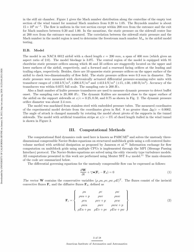
Also a limit number of kulite pressure transducers are used to measure dynamic pressure to detect buffetonset. The sampling rate is 20, 000 Hz. The dynamic Kulites are mounted close to the upper surface ofthe airfoil on the support sidewalls at x/c = 0.25, 0.50, and 0.75 as shown in Fig. 2. The dynamic pressureorifice diameter was about 2.4 mm.

The model was machined from stainless steel with embedded pressure tubes. The measured coordinatesof the experimental model deviate from the coordinates given in Ref. 8 no greater than ∆y/c = 0.0002.The angle of attack is changed manually by rotating the model about pivots of the supports in the tunnelsidewalls. The model with artificial transition strips at x/c = 5% of chord length italled in the wind tunnelis shown in Figure 3.

III. Computational Methods

The computational fluid dynamics code used here is known as PARCAE9 and solves the unsteady three-dimensional compressible Navier-Stokes equations on structured multiblock grids using a cell-centered finite-volume method with artificial dissipation as proposed by Jameson et al.10 Information exchange for flowcomputation on multiblock grids using multiple CPUs is implemented through the MPI (Message PassingInterface) protocol. The Navier-Stokes equations are solved using the eddy viscosity type turbulence models.All computations presented in this work are performed using Menter SST k-ω model.11 The main elementsof the code are summarized below.

The differential governing equations for the unsteady compressible flow can be expressed as follows:

∂W

∂t+ •(Fc − Fd) = 0 (1)

The vector W contains the conservative variables (ρ, ρu, ρv, ρw, ρE)T. The fluxes consist of the inviscidconvective fluxes Fc and the diffusive fluxes Fd, defined as

Fc =

ρu ρv ρw

ρuu + p ρuv ρuw

ρvu ρvv + p ρvw

ρwu ρwv ρww + p

ρEu + pu ρEv + pv ρEw + pw

(2)

3 of 18

American Institute of Aeronautics and Astronautics

Dow

nloa

ded

by U

NIV

ER

SIT

Y O

F C

AL

IFO

RN

IA I

RV

INE

on

Janu

ary

29, 2

015

| http

://ar

c.ai

aa.o

rg |

DO

I: 1

0.25

14/6

.201

3-30

26

Fd =

0 0 0

τxx τxy τxz

τyx τyy τyz

τzx τzy τzz

Θx Θy Θz

(3)

withΘ = u : τ − (

µL

PrL+

µT

PrT) T (4)

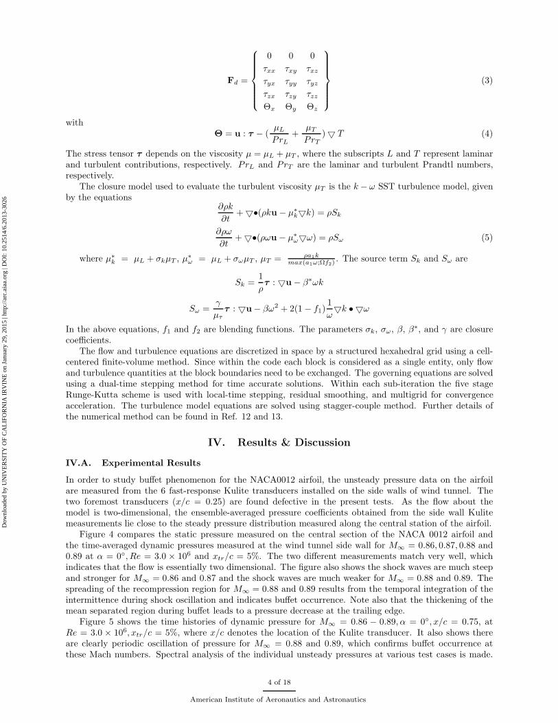
The stress tensor τ depends on the viscosity µ = µL + µT , where the subscripts L and T represent laminarand turbulent contributions, respectively. PrL and PrT are the laminar and turbulent Prandtl numbers,respectively.

The closure model used to evaluate the turbulent viscosity µT is the k − ω SST turbulence model, givenby the equations

∂ρk

∂t+ •(ρku − µ∗

kk) = ρSk

∂ρω

∂t+ •(ρωu− µ∗

ωω) = ρSω (5)

where µ∗k = µL + σkµT , µ∗

ω = µL + σωµT , µT = ρa1kmax(a1ω;Ωf2)

. The source term Sk and Sω are

Sk =1

ρτ : u − β∗ωk

Sω =γ

µττ : u− βω2 + 2(1 − f1)

1

ωk • ω

In the above equations, f1 and f2 are blending functions. The parameters σk, σω, β, β∗, and γ are closurecoefficients.

The flow and turbulence equations are discretized in space by a structured hexahedral grid using a cell-centered finite-volume method. Since within the code each block is considered as a single entity, only flowand turbulence quantities at the block boundaries need to be exchanged. The governing equations are solvedusing a dual-time stepping method for time accurate solutions. Within each sub-iteration the five stageRunge-Kutta scheme is used with local-time stepping, residual smoothing, and multigrid for convergenceacceleration. The turbulence model equations are solved using stagger-couple method. Further details ofthe numerical method can be found in Ref. 12 and 13.

IV. Results & Discussion

IV.A. Experimental Results

In order to study buffet phenomenon for the NACA0012 airfoil, the unsteady pressure data on the airfoilare measured from the 6 fast-response Kulite transducers installed on the side walls of wind tunnel. Thetwo foremost transducers (x/c = 0.25) are found defective in the present tests. As the flow about themodel is two-dimensional, the ensemble-averaged pressure coefficients obtained from the side wall Kulitemeasurements lie close to the steady pressure distribution measured along the central station of the airfoil.

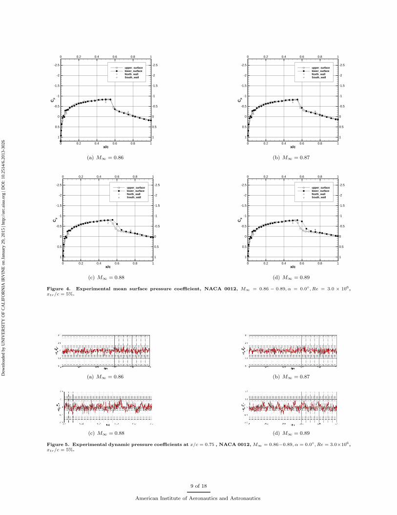
Figure 4 compares the static pressure measured on the central section of the NACA 0012 airfoil andthe time-averaged dynamic pressures measured at the wind tunnel side wall for M∞ = 0.86, 0.87, 0.88 and0.89 at α = 0, Re = 3.0 × 106 and xtr/c = 5%. The two different measurements match very well, whichindicates that the flow is essentially two dimensional. The figure also shows the shock waves are much steepand stronger for M∞ = 0.86 and 0.87 and the shock waves are much weaker for M∞ = 0.88 and 0.89. Thespreading of the recompression region for M∞ = 0.88 and 0.89 results from the temporal integration of theintermittence during shock oscillation and indicates buffet occurrence. Note also that the thickening of themean separated region during buffet leads to a pressure decrease at the trailing edge.

Figure 5 shows the time histories of dynamic pressure for M∞ = 0.86 − 0.89, α = 0, x/c = 0.75, atRe = 3.0 × 106, xtr/c = 5%, where x/c denotes the location of the Kulite transducer. It also shows thereare clearly periodic oscillation of pressure for M∞ = 0.88 and 0.89, which confirms buffet occurrence atthese Mach numbers. Spectral analysis of the individual unsteady pressures at various test cases is made.

4 of 18

American Institute of Aeronautics and Astronautics

Dow

nloa

ded

by U

NIV

ER

SIT

Y O

F C

AL

IFO

RN

IA I

RV

INE

on

Janu

ary

29, 2

015

| http

://ar

c.ai

aa.o

rg |

DO

I: 1

0.25

14/6

.201

3-30

26

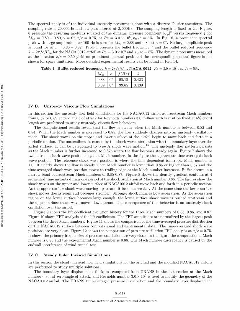
The spectral analysis of the individual unsteady pressures is done with a discrete Fourier transform. Thesampling rate is 20, 000Hz and low-pass filtered at 2, 000Hz. The sampling length is fixed to 2s. Figure.6 presents the resulting modulus squared of the dynamic pressure coefficient |Cp|

2 versus frequency f forM∞ = 0.80 − 0.89, α = 0, x/c = 0.75, at Re = 3.0 × 106, xtr/c = 5%. In Fig. 6, a prominent spectralpeak with large amplitude near 100 Hz is seen for M∞ = 0.88 and 0.89 at α = 0. No large amplitude peakis found for M∞ = 0.80 − 0.87. Table 1 presents the buffet frequency f and the buffet reduced frequencyk = 2πfc/U∞ for the NACA 0012 airfoil at Re = 3.0×106 and xtr/c = 5%. The dynamic pressures measuredat the location x/c = 0.50 yield no prominent spectral peak and the corresponding spectral figure is notshown for space limitation. More detailed experimental results can be found in Ref. 14.

Table 1. Buffet reduced frequency k = 2πfc/U∞, NACA 0012, Re = 3.0 × 106, xtr/c = 5%.

M∞ α f(Hz) k

0.88 0 95.15 0.423

0.89 0 99.65 0.439

IV.B. Unsteady Viscous Flow Simulations

In this section the unsteady flow field simulations for the NACA0012 airfoil at freestream Mach numbersfrom 0.82 to 0.89 at zero angle of attack for Reynolds numbers 3.0 million with transition fixed at 5% chordlength are performed to study unsteady viscous flow behaviors.

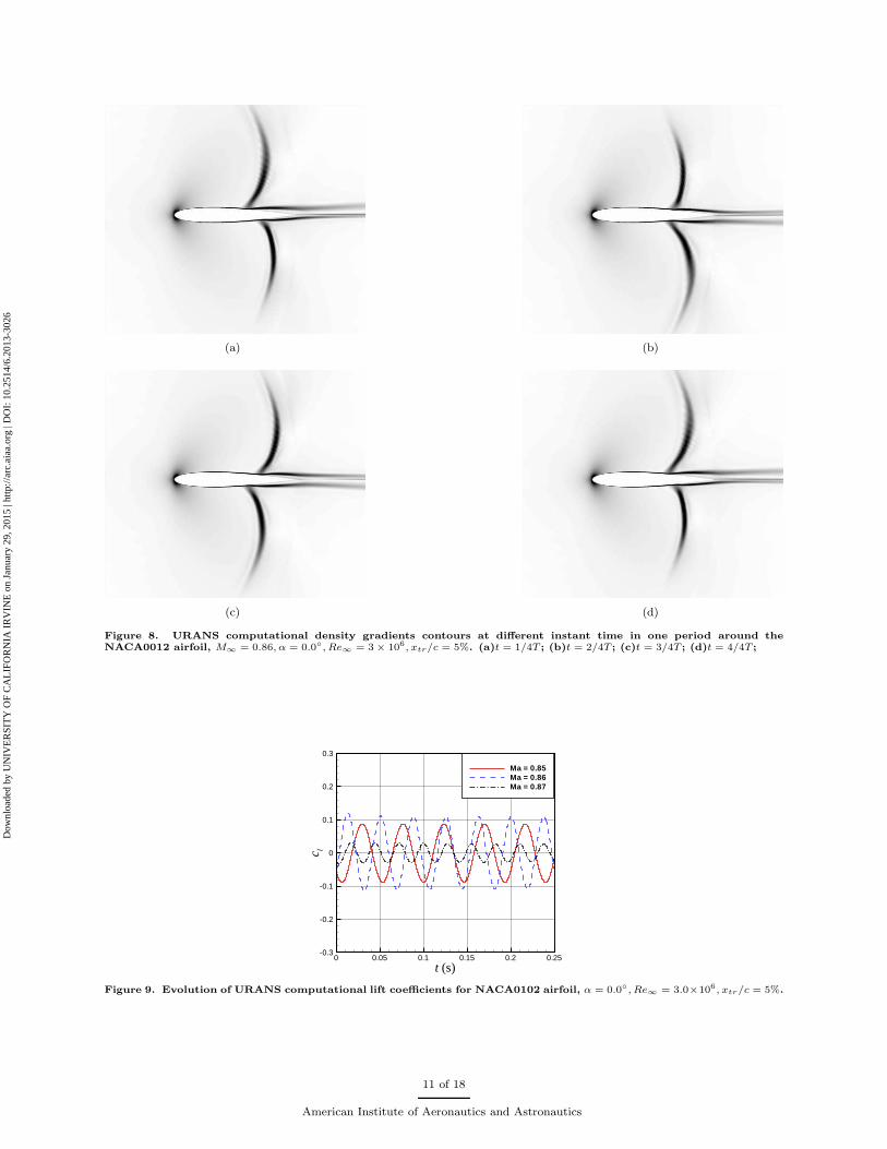
The computational results reveal that the flow is steady when the Mach number is between 0.82 and0.84. When the Mach number is increased to 0.85, the flow suddenly changes into an unsteady oscillatorymode. The shock waves on the upper and lower surfaces of the airfoil begin to move back and forth in aperiodic motion. The unsteadiness is caused by the shock wave interaction with the boundary layer over theairfoil surface. It can be categorized to type A shock wave motion.15 The unsteady flow pattern persistsas the Mach number is further increased to 0.875 where the flow becomes steady again. Figure 7 shows thetwo extreme shock wave positions against Mach number. In the figure the squares are time-averaged shockwave postion. The reference shock wave position is where the time dependent isentropic Mach number is1.0. It clearly shows the flow is steady when Mach number is lower than 0.85 or higher than 0.87 and thetime-averaged shock wave position moves to trailing edge as the Mach number increases. Buffet occurs in anarrow band of freestream Mach numbers of 0.85-0.87. Figure 8 shows the density gradient contours at 4sequential time instants during one period of the shock oscillation at Mach number 0.86. The figures show theshock waves on the upper and lower surface of NACA0012 airfoil move back and forth in a periodic motion.As the upper surface shock wave moving upstream, it becomes weaker. At the same time the lower surfaceshock moves downstream and becomes stronger. Stronger shock induces flow separation. As the separationregion on the lower surface becomes large enough, the lower surface shock wave is pushed upstream andthe upper surface shock wave moves downstream. The consequence of this behavior is an unsteady shockoscillation over the airfoil.

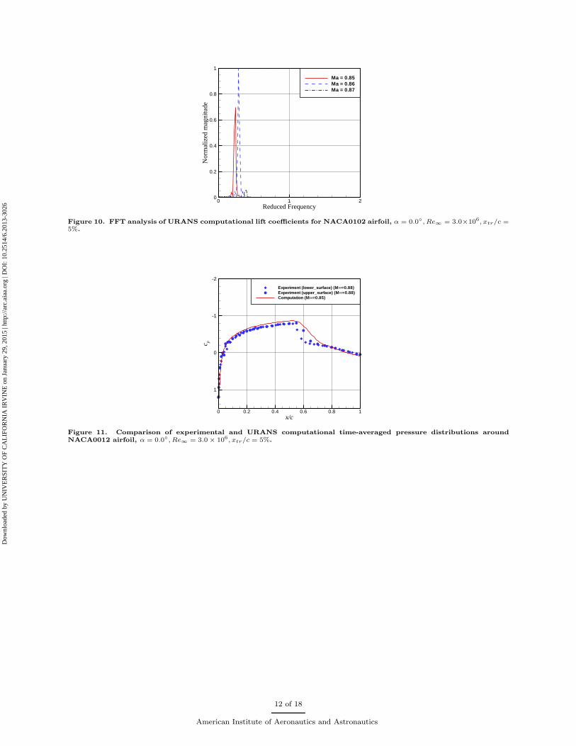
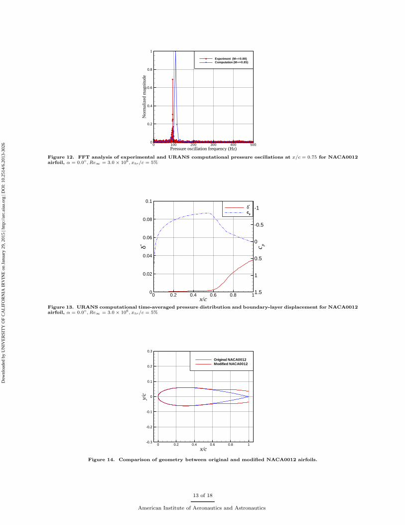
Figure 9 shows the lift coefficient evolution history for the three Mach numbers of 0.85, 0.86, and 0.87.Figure 10 shows FFT analysis of the lift coefficients. The FFT amplitudes are normalized by the largest peakbetween the three Mach numbers. Figure 11 shows the comparison of the time-averaged pressure distributionon the NACA0012 surface between computational and experimental data. The time-averaged shock wavepositions are very close. Figure 12 shows the comparison of pressure oscillation FFT analysis at x/c = 0.75.It shows the primary frequencies of pressure oscillation are very close. In the figure the computational Machnumber is 0.85 and the experimental Mach number is 0.88. The Mach number discrepancy is caused by theendwall interference of wind tunnel test.

IV.C. Steady Euler Inviscid Simulations

In this section the steady inviscid flow field simulations for the original and the modified NACA0012 airfoilsare performed to study multiple solutions.

The boundary layer displacement thickness computed from URANS in the last section at the Machnumber 0.86, at zero angle of attack, and Reynolds number 3.0× 106 is used to modify the geometry of theNACA0012 airfoil. The URANS time-averaged pressure distribution and the boundary layer displacement

5 of 18

American Institute of Aeronautics and Astronautics

Dow

nloa

ded

by U

NIV

ER

SIT

Y O

F C

AL

IFO

RN

IA I

RV

INE

on

Janu

ary

29, 2

015

| http

://ar

c.ai

aa.o

rg |

DO

I: 1

0.25

14/6

.201

3-30

26

thickness are plotted in Fig.13. Before the shock wave the boundary layer displacement thickness is verysmall. After the shock wave the boundary layer displacement thickness grows significantly, because the shockwave induces flow separation. Figure 14 shows the geometries of the original and the modified NACA0012airfoils. The rear port of modified airfoil is much thicker than the original NACA0012 airfoil. So the surfacesof the modified airfoil become flat and the tailing edge is not closed.

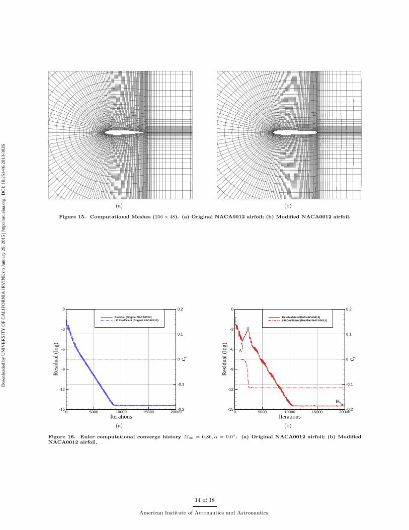
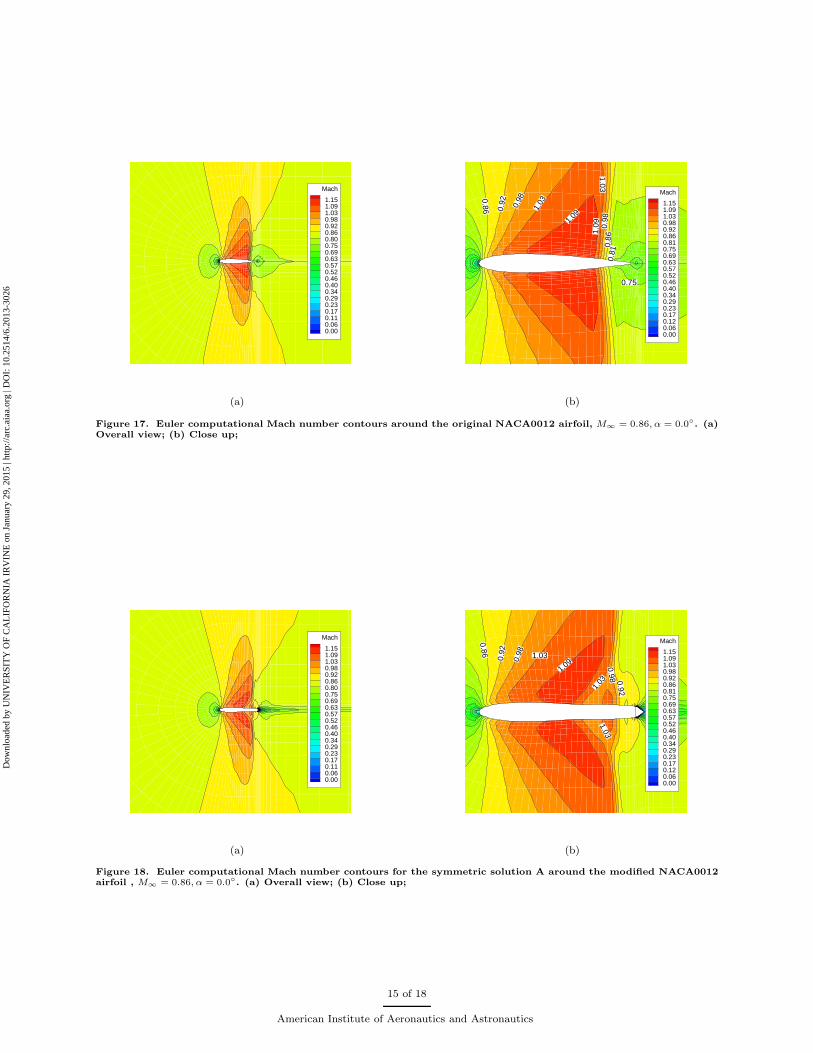
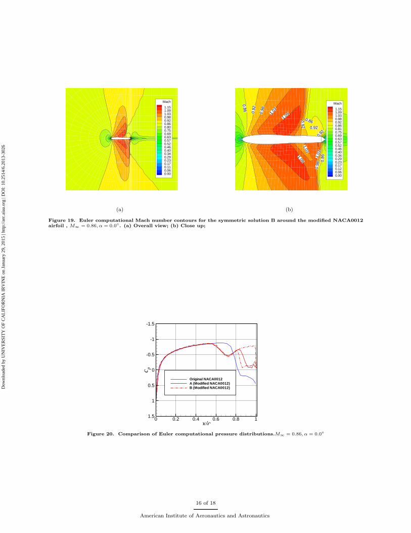
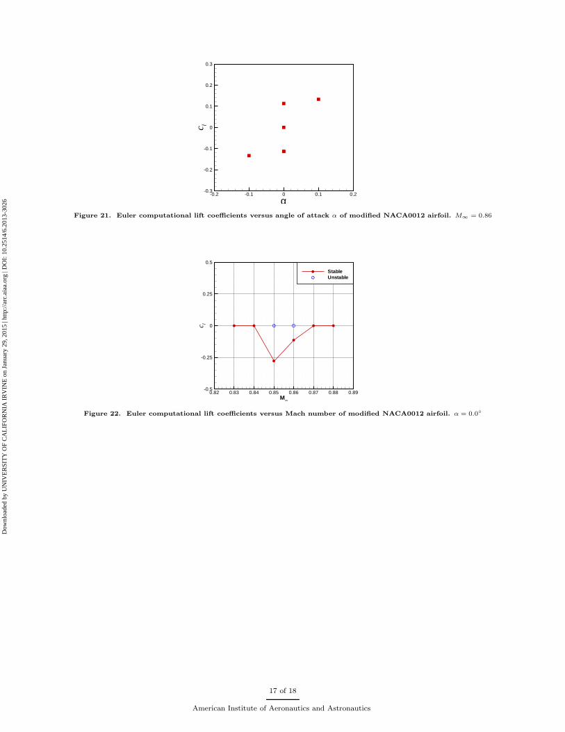
A C type mesh is generated for the inviscid computations. The mesh size is 257 × 49. Figure 15 showsthe computational meshes for both airfoils. In order to deal with the open tailing edge problem of modifiedairfoil, a ’transparent’ cusp tailing edge technique is used. Figure 16 shows the converging histories and liftcoefficients histories at M∞ = 0.86, α = 0. For original NACA0012 airfoil, the residual converges relativesmoothly to machine zero and the lift coefficients are zero during the iterations. It indicates the solution oforiginal NACA0012 airfoil at the flow condition is symmetric. While for the modified NACA0012 airfoil, theresidual firstly decreases to 5 orders. Then the residual jumps to a high level. After the jump the residualconverges to machine zero. The lift coefficient curve shows the solution is symmetric at the beginningand after the residual jump the solution becomes asymmetric. So there are two solutions for the modifiedNACA0012 airfoil at the flow condition M∞ = 0.86, α = 0. One is the symmetric solution A, and the otheris the asymmetric solution B. Figures 17 − 20 show the Mach number contours and pressure distributionsfor the original and the modified airfoils at M∞ = 0.86, α = 0. For the original NACA0012 airfoil, thesolution is symmetric. The shock wave occurs at 70% of chord length. For the modified airfoil, there aretwo solution A and B. For the symmetric solution A, the first shock wave occurs at 55% of chord lengthand followed by small expansion. The second shock wave occurs at 85% of chord length. Near the trailingedge there is another small expansion and compression caused by the thick tailing edge. For the asymmetricsolution B, also the first shock wave occurs at 55% of chord length and followed by small expansion. Thesecond shock wave moves to about 80% of chord length on the upper surface. On the lower surface thesecond shock wave moves to the tailing edge. The asymmetric second shock waves on the upper and lowersurface produce non-zero lift of the modified airfoil. Figure 21 shows the lift coefficients versus the angle ofattack for the modified NACA0012 airfoil at M∞ = 0.86. It shows there are 3 different solutions at zeroangle of attack. The different solutions are obtained by using different initial conditions. Figure 22 showsthe lift coefficients versus the Mach number for modified NACA0012 airfoil at zero angle of attack. It showsthe asymmetric solutions occurs at small range of Mach number M∞ = 0.85 − 0.86.

IV.D. Linear stability analysis

In this section the linear stability analysis is performed to analyze stability of the solutions of original andmodified NACA0012 airfoils at M∞ = 0.86, α = 0. In the analysis the flow field Jacobian matrix is obtainby perturbing the Euler equation residuals.16 The Euler equations can be expressed as follows:

∂W

∂t= R(W) (6)

The fourth-order accurate Jacobian matrix is

∂R

∂W=

1

12ǫd(−R(W + 2ǫd) + 8R(W + ǫd) − 8R(W − ǫd) + R(W − 2ǫd)) (7)

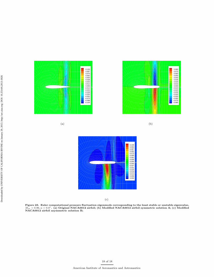
The discretized eigenvalue problem of a Jacobian matrix is solved using the implicit restarted Arnodimethod.17 The solution is achieved by using the ARPACK17 with the shift-invert mode. The prescribedfrequency is set to be zero which is the threshold of unsteadiness. The eigenvalues for the original NACA0012symmetric solution and the modified NACA0012 airfoil symmetric solution A and asymmetric solution B areexamined. For the original NACA0012 airfoil, all the eigenvalues have negative real parts which indicates thesolution is stable. The least stable eigenvalue has a real part of −0.0097. For the modified NACA0012 airfoilsymmetric solution A, the eigenvalue largest real part is positive 0.015. It means the symmetric solution A isunstable. For the modified NACA0012 airfoil asymmetric solution B, all the eigenvalues have negative realparts, which indicates the solution is stable. The least stable eigenvalue has a real part of −0.0092. Figure23 shows the pressure fluctuation eigenmodes corresponding to the least stable or unstable eigenvalue. Forthe original NACA0012 airfoil, the flow field is symmetric and the pressure fluctuation eigenmode is alsosymmetric. For the modified NACA0012 airfoil solution A, the flow field is symmetric, while the pressurefluctuation eigenmode is asymmetric. For solution B, the flow field and the pressure fluctuation eigenmodeare both asymmetric.

6 of 18

American Institute of Aeronautics and Astronautics

Dow

nloa

ded

by U

NIV

ER

SIT

Y O

F C

AL

IFO

RN

IA I

RV

INE

on

Janu

ary

29, 2

015

| http

://ar

c.ai

aa.o

rg |

DO

I: 1

0.25

14/6

.201

3-30

26

V. Conclusion

A combined experimental and computational study is performed to study buffet of the NACA0012 airfoiland its relation to inviscid multiple solutions. The experiments and computations both reveal that buffetappears under certain Reynolds number and transition position in a narrow Mach number range.

Boundary layer displacement thickness computed from URANS at the same flow condition is used tomodify the geometry of the NACA0012 airfoil. Euler equations are solved for the original and modified air-foils. For the original NACA0012 airfoil, there are no multiple solutions. While for the modified NACA0012airfoil, multiple solutions exist. The addition of the boundary layer displacement thickness creates multiplesolutions for the NACA0012 airfoil. Global linear stability analysis is performed on the original airfoil andthe modified airfoil. This shows a close relationship between the viscous unsteady shock buffet phenomenonof transonic airfoil flow and the existence of multiple solutions of the external inviscid flow. Buffet seems toappear when the external inviscid flow may exhibit multiple solutions and the mean flow field exhibit globalinstability.

References

1Liu, Y., Liu, F., and Luo, S., “Abstract: MX.00004 : Linear Stability Analysis on Multiple Solutions of Steady TransonicSmall Disturbance Equation,” APS, Nov. 2010.

2Steinhoff, J. and Jameson, A., “Multiple Solutions of Transonic Potential Flow Equation,” AIAA Journal , Vol. 20, No. 11,1982, pp. 1521–1525.

3Luo, S., Shen, H., and Liu, P., “Transonic Small Transverse Perturbation Equation and its Computation,” Proc. Sym-posium on Computing the Future II: Computational Fluid Dynamics Advances and Applications, ed. D. A. Caughey and M.M. Hafez, 1998.

4Salas, M. D., Jameson, A., and Melnik, R. E., “A Comparative Study of the Nonuniqueness problem of the PotentialEquation,” AIAA 1983-1888, July 1983.

5Williams, M. H., Bland, S. R., and Edwards, J. W., “Flow Instablities in Transonic Small-Disturbance Theory,” AIAA

Journal , Vol. 23, No. 10, 1985, pp. 1491–1496.6Crouch, J. D., Garbaruk, A., Magidov, D., and Travin, A., “Origin of Transonic Buffet on Aerofoil,” J. Fluid Mech.,

Vol. 628, 2009, pp. 357–369.7Xiong, J., Liu, F., and Luo, S., “Computation of NACA0012 Airfoil Transonic Buffet Phenomenon with Unsteady

Navier-Stokes Equations,” AIAA 2012-0699, January 2012.8Abbott, I. H. and Von Doenhoff, A. E., “Theory of Wing Sections,” Dover Publications, Inc., New York , 1959.9Xiong, J., Nielsen, P., Liu, F., and Papamoschou, D., “Computation of High-Speed Coaxial Jets with Fan Flow Deflec-

tion,” AIAA Journal , Vol. 48, No. 10, 2010, pp. 2249–2262.10Jameson, A., Schmift, W., and Turkel, E., “Numerical Solutions of the Euler Equations by Finite Volume Methods Using

Runge-Kutta Time Stepping Schemes,” AIAA 1981-1259, Janurary 1981.11Menter, F., “Two-Equation Eddy-Viscosity Turbulence Models for Engineering Applications,” AIAA Journal , Vol. 32,

No. 8, 1994, pp. 1598–1605.12Liu, F. and Zheng, X., “A Strongly Coupled Time-Marching Method for Solving the Navier-Stokes and k-ω Turbulence

Model Equations with Multigrid,” Journal of Computational Physics, Vol. 128, No. 10, 1996, pp. 257–284.13Xiao, Q., Tsai, H. M., and Liu, F., “Numerical Study of Transonic Buffet on a Supercritical Airfoil,” AIAA Journal ,

Vol. 44, No. 3, 2006, pp. 620–628.14Ren, X. and Zhao, Z. e. a., “Investigation of NACA 0012 airfoil Periodic Flows in a Transonic Wind Tunnel,” AIAA

2013-0791, January 2013.15Tijdeman, H. and Seebass, R., “Transonic Flow Past Oscillating Airfoils,” Annu. Rev. Fluid Mech., Vol. 12, 1980,

pp. 181–222.16Eriksson, L. E. and Rizzi, A., “Computer-Aided Analysis of the Convergence to Steady state of Discrete Approxiamtes

to the Euler Equations,” Journal of Computational Physics, Vol. 57, 1985, pp. 90–128.17Lehoucq, R. B., Sorenen, D. C., and Yang, C., “ARPACK User’s Guide,” SIAM Publication, 1998.

7 of 18

American Institute of Aeronautics and Astronautics

Dow

nloa

ded

by U

NIV

ER

SIT

Y O

F C

AL

IFO

RN

IA I

RV

INE

on

Janu

ary

29, 2

015

| http

://ar

c.ai

aa.o

rg |

DO

I: 1

0.25

14/6

.201

3-30

26

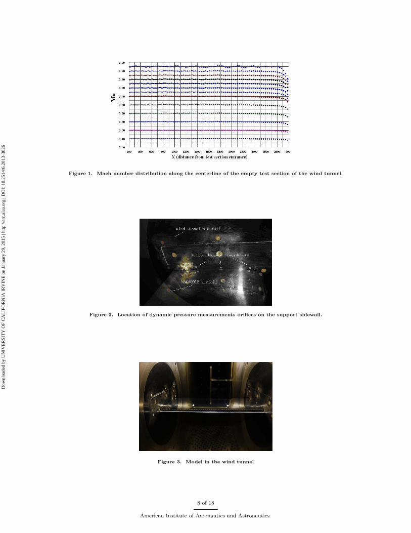
Figure 1. Mach number distribution along the centerline of the empty test section of the wind tunnel.

Figure 2. Location of dynamic pressure measurements orifices on the support sidewall.

Figure 3. Model in the wind tunnel

8 of 18

American Institute of Aeronautics and Astronautics

Dow

nloa

ded

by U

NIV

ER

SIT

Y O

F C

AL

IFO

RN

IA I

RV

INE

on

Janu

ary

29, 2

015

| http

://ar

c.ai

aa.o

rg |

DO

I: 1

0.25

14/6

.201

3-30

26

x/c

Cp

0

0

0.2

0.2

0.4

0.4

0.6

0.6

0.8

0.8

1

1

-2.5 -2.5

-2 -2

-1.5 -1.5

-1 -1

-0.5 -0.5

0 0

0.5 0.5

1 1

upper_surfacelower_surfaceNorth_wallSouth_wall

(a) M∞ = 0.86

x/c

Cp

0

0

0.2

0.2

0.4

0.4

0.6

0.6

0.8

0.8

1

1

-2.5 -2.5

-2 -2

-1.5 -1.5

-1 -1

-0.5 -0.5

0 0

0.5 0.5

1 1

upper_surfacelower_surfaceNorth_wallSouth_wall

(b) M∞ = 0.87

x/c

Cp

0

0

0.2

0.2

0.4

0.4

0.6

0.6

0.8

0.8

1

1

-2.5 -2.5

-2 -2

-1.5 -1.5

-1 -1

-0.5 -0.5

0 0

0.5 0.5

1 1

upper_surfacelower_surfaceNorth_wallSouth_wall

(c) M∞ = 0.88

x/c

Cp

0

0

0.2

0.2

0.4

0.4

0.6

0.6

0.8

0.8

1

1

-2.5 -2.5

-2 -2

-1.5 -1.5

-1 -1

-0.5 -0.5

0 0

0.5 0.5

1 1

upper_surfacelower_surfaceNorth_wallSouth_wall

(d) M∞ = 0.89

Figure 4. Experimental mean surface pressure coefficient, NACA 0012, M∞ = 0.86 − 0.89, α = 0.0, Re = 3.0 × 106,xtr/c = 5%.

(a) M∞ = 0.86 (b) M∞ = 0.87

(c) M∞ = 0.88 (d) M∞ = 0.89

Figure 5. Experimental dynamic pressure coefficients at x/c = 0.75 , NACA 0012, M∞ = 0.86−0.89, α = 0.0, Re = 3.0×106,xtr/c = 5%.

9 of 18

American Institute of Aeronautics and Astronautics

Dow

nloa

ded

by U

NIV

ER

SIT

Y O

F C

AL

IFO

RN

IA I

RV

INE

on

Janu

ary

29, 2

015

| http

://ar

c.ai

aa.o

rg |

DO

I: 1

0.25

14/6

.201

3-30

26

f(Hz)0

200400

600800

10001200

14001600

18002000

M exp

0.80.81

0.820.83

0.840.85

0.860.87

0.880.89

|cp|2

(Hz- 2

)

0

2E-05

4E-05

6E-05

8E-05

0.0001

∧

Figure 6. Experimental dynamic pressure coefficient modulus squared |Cp|2 vs. frequency f , NACA 0012, M∞ =

0.80 0.89, α = 0, x/c = 0.75,Re = 3.0 × 106, xtr/c = 5%.

M∞

x s/c

0.82 0.84 0.86 0.88 0.90.5

0.6

0.7

0.8

0.9

1

Figure 7. URANS computational shock wave position against freestream Mach number for NACA0012 airfoil, α =0.0, Re∞ = 3.0 × 106, xtr/c = 5%. (Blue square denotes time-averaged shock wave position)

10 of 18

American Institute of Aeronautics and Astronautics

Dow

nloa

ded

by U

NIV

ER

SIT

Y O

F C

AL

IFO

RN

IA I

RV

INE

on

Janu

ary

29, 2

015

| http

://ar

c.ai

aa.o

rg |

DO

I: 1

0.25

14/6

.201

3-30

26

(a) (b)

(c) (d)

Figure 8. URANS computational density gradients contours at different instant time in one period around theNACA0012 airfoil, M∞ = 0.86, α = 0.0, Re∞ = 3 × 106, xtr/c = 5%. (a)t = 1/4T ; (b)t = 2/4T ; (c)t = 3/4T ; (d)t = 4/4T ;

t (s)

c l

0 0.05 0.1 0.15 0.2 0.25-0.3

-0.2

-0.1

0

0.1

0.2

0.3

Ma = 0.85Ma = 0.86Ma = 0.87

Figure 9. Evolution of URANS computational lift coefficients for NACA0102 airfoil, α = 0.0, Re∞ = 3.0×106, xtr/c = 5%.

11 of 18

American Institute of Aeronautics and Astronautics

Dow

nloa

ded

by U

NIV

ER

SIT

Y O

F C

AL

IFO

RN

IA I

RV

INE

on

Janu

ary

29, 2

015

| http

://ar

c.ai

aa.o

rg |

DO

I: 1

0.25

14/6

.201

3-30

26

Reduced FrequencyN

orm

aliz

edm

agni

tude

0 1 20

0.2

0.4

0.6

0.8

1

Ma = 0.85Ma = 0.86Ma = 0.87

Figure 10. FFT analysis of URANS computational lift coefficients for NACA0102 airfoil, α = 0.0, Re∞ = 3.0×106, xtr/c =5%.

x/c

c p

0 0.2 0.4 0.6 0.8 1

-2

-1

0

1

Experiment (lower_surface) (M ∞=0.88)Experiment (upper_surface) (M ∞=0.88)Computation (M ∞=0.85)

Figure 11. Comparison of experimental and URANS computational time-averaged pressure distributions aroundNACA0012 airfoil, α = 0.0, Re∞ = 3.0 × 106, xtr/c = 5%.

12 of 18

American Institute of Aeronautics and Astronautics

Dow

nloa

ded

by U

NIV

ER

SIT

Y O

F C

AL

IFO

RN

IA I

RV

INE

on

Janu

ary

29, 2

015

| http

://ar

c.ai

aa.o

rg |

DO

I: 1

0.25

14/6

.201

3-30

26

Pressure oscillation frequency (Hz)N

orm

aliz

edm

agni

tude

0 100 200 300 400 5000

0.2

0.4

0.6

0.8

1

Experiment (M ∞=0.88)Computation (M ∞=0.85)

Figure 12. FFT analysis of experimental and URANS computational pressure oscillations at x/c = 0.75 for NACA0012airfoil, α = 0.0, Re∞ = 3.0 × 106, xtr/c = 5%

x/c

δ* c p

0 0.2 0.4 0.6 0.8 10

0.02

0.04

0.06

0.08

0.1

-1

-0.5

0

0.5

1

1.5

δ*

cp

Figure 13. URANS computational time-averaged pressure distribution and boundary-layer displacement for NACA0012airfoil, α = 0.0, Re∞ = 3.0 × 106, xtr/c = 5%

x/c

y/c

0 0.2 0.4 0.6 0.8 1-0.3

-0.2

-0.1

0

0.1

0.2

0.3

Original NACA0012Modified NACA0012

Figure 14. Comparison of geometry between original and modified NACA0012 airfoils.

13 of 18

American Institute of Aeronautics and Astronautics

Dow

nloa

ded

by U

NIV

ER

SIT

Y O

F C

AL

IFO

RN

IA I

RV

INE

on

Janu

ary

29, 2

015

| http

://ar

c.ai

aa.o

rg |

DO

I: 1

0.25

14/6

.201

3-30

26

(a) (b)

Figure 15. Computational Meshes (256 × 48). (a) Original NACA0012 airfoil; (b) Modified NACA0012 airfoil.

Iterations

Res

idua

l(lo

g)

c l

0 5000 10000 15000 20000-15

-12

-9

-6

-3

0

-0.2

-0.1

0

0.1

0.2

Residual (Original NACA0012)Lift Coefficient (Original NACA0012)

(a)

Iterations

Res

idua

l(lo

g)

c l

0 5000 10000 15000 20000-15

-12

-9

-6

-3

0

-0.2

-0.1

0

0.1

0.2

Residual (Modified NACA0012)Lift Coefficient (Modified NACA0012)

A

B

(b)

Figure 16. Euler computational converge history M∞ = 0.86, α = 0.0. (a) Original NACA0012 airfoil; (b) ModifiedNACA0012 airfoil.

14 of 18

American Institute of Aeronautics and Astronautics

Dow

nloa

ded

by U

NIV

ER

SIT

Y O

F C

AL

IFO

RN

IA I

RV

INE

on

Janu

ary

29, 2

015

| http

://ar

c.ai

aa.o

rg |

DO

I: 1

0.25

14/6

.201

3-30

26

Mach

1.151.091.030.980.920.860.800.750.690.630.570.520.460.400.340.290.230.170.110.060.00

(a)

0.86 0.92 0.98

1.03

1.09

1.09

1.03

0.98

0.86

0.81

0.75

Mach

1.151.091.030.980.920.860.810.750.690.630.570.520.460.400.340.290.230.170.120.060.00

(b)

Figure 17. Euler computational Mach number contours around the original NACA0012 airfoil, M∞ = 0.86, α = 0.0. (a)Overall view; (b) Close up;

Mach

1.151.091.030.980.920.860.800.750.690.630.570.520.460.400.340.290.230.170.110.060.00

(a)

0.86

0.92

0.98 1.03

1.09

1.03

1.030.98 0.92

Mach

1.151.091.030.980.920.860.810.750.690.630.570.520.460.400.340.290.230.170.120.060.00

(b)

Figure 18. Euler computational Mach number contours for the symmetric solution A around the modified NACA0012airfoil , M∞ = 0.86, α = 0.0. (a) Overall view; (b) Close up;

15 of 18

American Institute of Aeronautics and Astronautics

Dow

nloa

ded

by U

NIV

ER

SIT

Y O

F C

AL

IFO

RN

IA I

RV

INE

on

Janu

ary

29, 2

015

| http

://ar

c.ai

aa.o

rg |

DO

I: 1

0.25

14/6

.201

3-30

26

Mach

1.151.091.030.980.920.860.800.750.690.630.570.520.460.400.340.290.230.170.110.060.00

(a)

0.86

0.92

0.98

1.03

1.090.92

1.03

0.86

0.92

1.03

0.98

0.861.09

0.92

Mach

1.151.091.030.980.920.860.810.750.690.630.570.520.460.400.340.290.230.170.120.060.00

(b)

Figure 19. Euler computational Mach number contours for the symmetric solution B around the modified NACA0012airfoil , M∞ = 0.86, α = 0.0. (a) Overall view; (b) Close up;

x/c

c p

0 0.2 0.4 0.6 0.8 1

-1.5

-1

-0.5

0

0.5

1

1.5

Original NACA0012A (Modified NACA0012)B (Modified NACA0012)

Figure 20. Comparison of Euler computational pressure distributions.M∞ = 0.86, α = 0.0

16 of 18

American Institute of Aeronautics and Astronautics

Dow

nloa

ded

by U

NIV

ER

SIT

Y O

F C

AL

IFO

RN

IA I

RV

INE

on

Janu

ary

29, 2

015

| http

://ar

c.ai

aa.o

rg |

DO

I: 1

0.25

14/6

.201

3-30

26

αc l

-0.2 -0.1 0 0.1 0.2-0.3

-0.2

-0.1

0

0.1

0.2

0.3

Figure 21. Euler computational lift coefficients versus angle of attack α of modified NACA0012 airfoil. M∞ = 0.86

M∞

c l

0.82 0.83 0.84 0.85 0.86 0.87 0.88 0.89-0.5

-0.25

0

0.25

0.5

StableUnstable

Figure 22. Euler computational lift coefficients versus Mach number of modified NACA0012 airfoil. α = 0.0

17 of 18

American Institute of Aeronautics and Astronautics

Dow

nloa

ded

by U

NIV

ER

SIT

Y O

F C

AL

IFO

RN

IA I

RV

INE

on

Janu

ary

29, 2

015

| http

://ar

c.ai

aa.o

rg |

DO

I: 1

0.25

14/6

.201

3-30

26

0.1000.0870.0750.0620.0500.0380.0250.0120.000

-0.012-0.025-0.038-0.050-0.062-0.075-0.088-0.100

(a)

0.0800.0700.0600.0500.0400.0300.0200.0100.000

-0.010-0.020-0.030-0.040-0.050-0.060-0.070-0.080

(b)

0.1000.0940.0870.0810.0750.0690.0620.0560.0500.0440.0370.0310.0250.0190.0130.0060.000

(c)

Figure 23. Euler computational pressure fluctuation eigenmode corresponding to the least stable or unstable eigenvalue,M∞ = 0.86, α = 0.0. (a) Original NACA0012 airfoil; (b) Modified NACA0012 airfoil symmetric solution A; (c) ModifiedNACA0012 airfoil asymmetric solution B;

18 of 18

American Institute of Aeronautics and Astronautics

Dow

nloa

ded

by U

NIV

ER

SIT

Y O

F C

AL

IFO

RN

IA I

RV

INE

on

Janu

ary

29, 2

015

| http

://ar

c.ai

aa.o

rg |

DO

I: 1

0.25

14/6

.201

3-30

26