HAL Id: hal-02907472https://hal.archives-ouvertes.fr/hal-02907472

Submitted on 7 Dec 2020

HAL is a multi-disciplinary open accessarchive for the deposit and dissemination of sci-entific research documents, whether they are pub-lished or not. The documents may come fromteaching and research institutions in France orabroad, or from public or private research centers.

L’archive ouverte pluridisciplinaire HAL, estdestinée au dépôt et à la diffusion de documentsscientifiques de niveau recherche, publiés ou non,émanant des établissements d’enseignement et derecherche français ou étrangers, des laboratoirespublics ou privés.

Multiple Site-Specific Phosphorylation of IDPsMonitored by NMR

Manon Julien, Chafiaa Bouguechtouli, Ania Alik, Rania Ghouil, SophieZinn-Justin, François-Xavier Theillet

To cite this version:Manon Julien, Chafiaa Bouguechtouli, Ania Alik, Rania Ghouil, Sophie Zinn-Justin, et al.. MultipleSite-Specific Phosphorylation of IDPs Monitored by NMR. Intrinsically Disordered Proteins, 2141(26), pp.793–817, 2020, �10.1007/978-1-0716-0524-0_41�. �hal-02907472�

1

Multiple Site-specific Phosphorylation of IDPs Monitored by NMR

Manon Julien1, Chafiaa Bouguechtouli

1, Ania Alik

1, Rania Ghouil

1, Sophie Zinn-Justin

1, François-

Xavier Theillet1*

Affiliation: 1

Institute for Integrative Biology of the Cell (I2BC), CEA, CNRS, Univ Paris-Sud,

Université Paris-Saclay, Gif-sur-Yvette Cedex, France.

*Corresponding author. E-mail address: francois-xavier.theillet@cnrs.fr

Running head: IDP phosphorylation monitored by NMR.

2

Abstract

In line with their high accessibility, disordered proteins are exquisite targets of kinases. Eukaryotic

organisms use the so-called intrinsically disordered proteins (IDPs) or intrinsically disordered

regions of proteins (IDRs) as molecular switches carrying intracellular information tuned by

reversible phosphorylation schemes. Solvent exposed serines and threonines are abundant in

IDPs, and, consistently, kinases often modify disordered regions of proteins at multiple sites. In

this context, nuclear magnetic resonance (NMR) spectroscopy provides quantitative, residue-

specific information that permits mapping of phosphosites and monitoring of their individual

kinetics. Hence, NMR monitoring emerges as an in vitro approach, complementary to mass-

spectrometry or immuno-blotting, to characterize IDP phosphorylation comprehensively. Here, we

describe in detail generic protocols for carrying out NMR monitoring of IDP phosphorylation, and

we provide a number of practical insights that improve handiness and reproducibility of this

method.

Key words

NMR spectroscopy, Intrinsically Disordered Proteins, IDP, post-translational modifications,

phosphorylation, cell signaling, kinases, multiple phosphosites, quantitative NMR, time-resolved

NMR.

3

1. Introduction

Living organisms use post-translational modifications (PTMs) as a convenient mechanism to

transmit information in a fast and reversible fashion. PTMs can provoke changes in protein

conformation or create/abolish binding sites, therefore regulating the activity of proteins. In

eukaryotes, serine/threonine phosphorylation represents about 60% of the detected PTMs [1, 2].

Intrinsically disordered regions (IDRs) of proteins carry ~60% of the ~200,000 phosphosites

found in the 13,000 human phosphoproteins [3, 4], in line with their importance in cell signaling

[5]. Interestingly, phosphosites tend to cluster : about half of them are at a distance of four

residues or less [6], while more than 50% of phosphoproteins have six phosphosites or more [7].

This generates potential crosstalks, collective effects and improved robustness of signaling [5, 8-

10]. A large number of detected phosphorylation sites may also reveal loose specificities that

result from the promiscuous access of kinases to IDP residues [11]: a majority of the detected

phosphosites in cultured cells show a fractional occupancy of 25% or less, the functional role of

such events being unclear [7, 12].

The most popular methods to detect phosphorylation are mass-spectrometry and Western-

blotting, because of their ability to detect phosphosites in biological material with high sensitivity.

However, multiple neighboring phosphorylation sites hamper immuno-recognition and prevent

standard peptide isolation/enrichment/ionization/identification steps in the course of MS analysis,

although technical advances have been achieved in this field [13]. Degenerate motifs are also

problematic in western-blotting because they hinder site-specific immuno-recognition. Finally,

improving phosphoproteome coverage is a perpetual battle: even though novel buffers,

enrichment methods, chromatography, and digestion protocols progressively enhance sampling

depth [14, 15], accessible data from immunoblots and MS can probably not provide a

comprehensive view of the PTM schemes established on your protein of interest.

NMR spectroscopy is a complementary method, because of its intrinsic ability to provide

quantitative, residue-specific information on IDPs in solution [16]. Using the “NMR isotope-filter”,

15N-labeled proteins are the only observable species in the presence of natural abundance

14N-

containing material, which makes it possible to monitor phosphorylation reactions of a 15

N-labeled

4

IDP in vitro and in cell extracts [17, 18]. For example, it has been instrumental to solve complex

phosphorylation cascades on PTEN [19], or to elucidate the respective kinetics and roles of

degenerated Erk phosphosites on Elk1 [20].

NMR spectroscopy provides residue-specific information because nuclei resonance frequencies

depend on their chemical environment. Upon phosphorylation, the chemical environment

changes in the vicinity of the phosphorylated residues, provoking new chemical shifts for residues

neighboring the phosphosites. We illustrate it here with the example of a BRCA2 fragment (aa48-

218), phosphorylated at S193 and T207, which generates large chemical shift perturbations for

S193 and T207, but also weak but discernable NMR signals displacements of their neighboring

residues D189, S195, L198, A199, T203 and V211 (Fig. 1a) [16, 21]. Hence, by recording time

series of NMR spectra during the phosphorylation reactions, we can obtain time-resolved

quantification or reaction advancement at every phosphosite: new crosspeaks appear while some

peaks progressively disappear, corresponding to phosphorylated and non-modified populations,

respectively (Fig. 1b). More complex situations can emerge when close residues are

concomitantly phosphorylated: two neighboring sites S1 and S2 (separated by ~4-6 amino acids

or less) will generate a set of four peaks upon phosphorylation, corresponding to S1-S2, pS1-S2,

S1-pS2 and pS1-pS2, where pS1-S2 and S1-pS2 peaks may increase and later decrease (see

for example [19, 22, 23]).

In the past years, we have successfully monitored phosphorylation reactions using NMR on a

large variety of IDPs and kinases. Here, we provide a generic protocol integrating a sum of

technical solutions focusing on sample preparation, control of the reaction conditions and

instrument parameters for generating reliable data. We also provide some explanations for the

rationale and warnings to avoid misinterpretation (see Note 1). We illustrate the protocol with

results obtained on a BRCA2 fragment (aa48-218) phosphorylated by Plk1.

[Fig 1 near here]

2. Materials

5

2.1 Stock Solutions Preparation and Storage

Prepare all solutions using milli-Q water (resistivity of 18.2 MΩ*cm at 25 °C). Buffers, reagents

stocks and proteins can be kept at -20°C for months, but fresh dithiothreitol (DTT) or tris(2-

carboxyethyl)phosphine (TCEP) should be added to the samples before performing experiments.

DTT half-life in solution is indeed about one day at pH~7 and even decreases in presence of

metal ions [24] so that buffers containing DTT should not be stored. Other reducing agents may

be used with profit but also with careful attention (see Note 2).

We describe standard buffers using Hepes at 50 mM, pH 7.0. Any good buffering molecule in this

range of pH would also be acceptable, e.g. phosphate, PIPES, MOPS, whose pKas also have

low temperature coefficients (see Note 3).

1. Standard IDP Size-Exclusion Chromatography (SEC) buffer (SEC-B): 50 mM Hepes, 100

mM NaCl, pH 7.0.

2. Standard IDP frozen storage buffer (Stor-B): 50 mM Hepes, 100 mM NaCl, pH 7.0, 2 mM

DTT, 1x ethylenediaminetetraacetic acid (EDTA)-free protease inhibitors.

3. Standard phosphorylation buffer (Phos-B): 50 mM Hepes, 100 mM NaCl, pH 7.0, 4 mM

DTT, 1x EDTA-free protease inhibitors, 4 mM adenosine triphosphate (ATP), 10 mM MgCl2.

4. Urea buffer (UB): 50 mM Hepes, 100 mM NaCl, pH 6.5, 4 mM DTT, 10 M urea. High urea

concentration buffers tend to progressively diverge towards higher pH when stored at room

temperature for days.

5. ATP stock solution: 0.1 M ATP, pH 7.0 in water (10 mM Hepes can be added for

convenient pH adjustment); store aliquots at -20 °C.

6. DTT stock solution: 1 M DTT in water; store aliquots at -20 °C.

7. MgCl2 stock solution: 1 M MgCl2, pH 7.0 (10 mM Hepes can be added for convenient pH

adjustment); store aliquots at -20 °C.

8. EDTA-free proteases inhibitors (PI): prepare a 25x stock solution (cOmplete EDTA-free

tablets, or any other cocktail of inhibitors that does not contain EDTA). Store aliquots at -20 °C.

6

9. 15

N-labeled IDP stock solution at a concentration greater than or equal to 200-250 M is

stored at -80 °C. Aliquoting prevents eventual aggregation that often appears upon multiple

freeze-thaw cycles.

10. Kinase stock solution: active kinase is obtained either commercially or produced in-house.

Prepare low volumes aliquots on ice (2 to 10 L, providing a phosphate transfer activity in the

range of 50 to 500 pmol/min) and flash-freeze them before storage at -80 °C. Aliquoting

preserves kinase activity with may be lost upon freeze-thaw cycles, and will thus favor

experimental reproducibility. Addition of 20 % glycerol promotes activity conservation.

11. EDTA or trans-1,2-Diaminocyclohexane-N,N,N′,N′-tetraacetic acid monohydrate (CyDTA)

stock solution: 0.5 M EDTA or CyDTA solution, pH 7.0; store aliquots at -20 °C.

12. D2O at 99% deuterium enrichment.

13. 4,4-dimethyl-4-silapentane-1-sulfonic acid (DSS) stock solution: 100 mM DSS in water;

store at room temperature (RT).

14. Laemmli buffer 4x: 10 mL Tris (1 M, pH 6.8), 4 g sodium dodecyl sulfate (SDS), 20 mL

glycerol, 10 mL -mercaptoethanol, 0.1 g bromophenol blue, 6 mL H2O.

15. Polyacrylamide gels for SDS-PAGE analysis.

2.2 Sample Preparation

1. SEC column: preparative 16/600 Superdex column containing 75pg or 200pg resin

depending on protein size.

2. Fast protein liquid chromatography (FPLC) system at 4 °C able to carry out SEC, i.e.

applying constant flow rates of 0.3-1.5 mL/min at a pressure of 0.15 to 0.5 MPa.

3. 0.22 m pore-size membrane filter system.

4. Centrifugal concentrators with a pore size adapted to the IDP molecular weight.

5. Precise pH-meter combined with a pH microelectrode able to measure pH in ~100 L

samples.

2.3 NMR Spectra Acquisition and Analysis

7

1. High-field NMR spectrometer (larger or equal to 600 MHz) equipped with a triple-

resonance cryoprobe.

2. A 1H-

15N SOFAST-HMQC pulse sequence program. This can be found in most of the

standard pulse sequence libraries. Be careful with the default pulses used in libraries: the central

band-selective 180° pulse should be a REBURP and not a r-SNOB to get maximal S/N, as shown

by Schanda et al. [25]. Set interscan delays to ~100 ms and use a high number of dummy scans

(>64). Set offset frequencies of shaped pulses to 8.5 ppm and use large pulse lengths (>2.4 ms)

to avoid saturation of water protons magnetization. Because of fast amide-water proton exchange

in IDPs, water protons represent a magnetization reservoir enhancing the apparent amide

interscan T1-recovery [26]. For this reason, great S/N enhancement is obtained for IDPs using

long shaped pulses at fields higher than 600-700 MHz, since amide and water proton frequencies

become distant enough.

3. A 1H-

15N HSQC pulse sequence program. Sensitivity enhanced versions of this pulse

sequence provide better S/N for most IDPs. This can be found in most of the standard pulse

sequence libraries.

4. NMR tubes. These can be 3 or 5 mm diameter regular tubes, which must be filled with

minimal volumes of 150 or 475 L, respectively. In standard phosphorylation buffer conditions, 5

mm tubes offer about twice S/N than 3 mm tubes. Using 3 or 5 mm diameter Shigemi tubes

optimizes sample efficiency by reducing sample volumes to 90 or 270 L, respectively. 4 mm

Shigemi tubes (efficient volume: 180 L) also exist.

5. NMR data processing and analysis softwares (e.g. Topspin, NMRPipe, CcpNmr Analysis,

Sparky, ...).

6. Plotting and fitting software (e.g. Prism, Kaleidagraph, Gnuplot, ..).

3. Methods

The following protocol describes a generic strategy to monitor IDP phosphorylation using NMR

spectroscopy. This requires the prior production and purification of the protein of interest

8

uniformly 15

N or 15

N/13

C labeled. Such labeling is usually obtained by recombinant protein

expression in bacteria (see Note 4). Bacterial expression is preferred for this protocol because it

generates recombinant, non-phosphorylated proteins in most cases (see Note 5). We will not

detail the corresponding tasks, but we must stress a few points that should be considered with

great care for later success in phosphorylation characterization. The IDP of interest can be

purified using standard strategies adapted to the presence or absence of affinity tags. First, to

avoid any artifactual influence of such tags, their cleavage and removal is generally preferred

before executing PTMs kinetics experiments. Second, because of their high accessibility, IDP’s

cysteines are prone to establish non-native disulfide bonds in vitro. The complete reduction of

cysteine thiols at every step of the purification is mandatory (see Note 2). Third, IDPs

susceptibility to proteolysis must be addressed by the addition of protease inhibitors in lysis buffer

and after every purification step.

The protocol starts with the last preparation steps of the IDP sample, then describes a method to

optimize the phosphorylation conditions, and later a method to assign the NMR spectra in the

phosphorylation conditions. The two final subsections detail the NMR data acquisition and

analysis. We have introduced two possible methods to record NMR spectra, either by a

continuous readout of a single sample during the phosphorylation reaction (3.4.1 NMR

continuous readout), or by successive measurements of aliquots quenched at various time points

(3.4.2 The “Quenched reaction” approach). The first approach is more convenient in many

aspects, but it provides too weak S/N for a number of IDPs (see Note 6). All other paragraphs are

common to all IDPs.

3.1. Preparation of the IDP Stock

We start the protocol with the last preparation step of the IDP, which consists of a SEC. This

permits i) to polish the protein purification and ii) to transfer the IDP into the exact salt and buffer

conditions used for the phosphorylation reaction.

9

1. Equilibrate the SEC column with two column-volumes of SEC-B, previously filtered on a

0.22 m pore-size membrane. Using an FPLC system at 4°C will lower the risks of IDP

proteolysis.

2. Concentrate the purified IDP to a final volume of 2 mL in the presence of 2 mM DTT and

PIs (final concentration 1x), using concentrators with centrifugation steps at 10 °C (4,000 x g for

swinging buckets, 5,000 x g for fixed angle rotors).

3. Add DTT to a final concentration of 10 mM DTT to the concentrated sample and incubate

it for 30 min at RT to ensure that all thiols are reduced.

4. Centrifuge the sample for 5 min at 16,000 x g and 4 °C to remove aggregates and inject

the supernatant on the equilibrated SEC column.

5. Run the SEC with parameters recommended by manufacturers and check the purity of

the eluted fractions by SDS-PAGE.

6. Pool the fractions of interest, supplement them with 2 mM DTT (final concentration) and

PIs (final concentration 1x), and concentrate the protein to 250 M by centrifugation at 10 °C

(4,000 x g for swinging buckets, 5,000 x g for fixed angle rotors).

7. Flash freeze the sample in liquid nitrogen and store it at -80 °C.

3.2. Optimization of Phosphorylation Conditions

For every IDP:kinase pair, phosphorylation kinetics can be first evaluated by SDS-PAGE in order

to identify the appropriate concentration of kinase and, eventually, the best buffer conditions. This

relies on the fact that phosphorylated amino acids tend to slow down protein migration during

SDS-PAGE (Fig. 2). SDS-binding to phosphoproteins is thought to be weaker, which provokes a

decreased electrophoretic mobility [27]. However, this effect can be negligible for proteins

carrying large excess (~15 or more) of negative charges due to a biased composition between

Glu/Asp and Arg/Lys; this situation calls for directly moving on to NMR monitoring. Here, we

describe the procedure for the SDS-PAGE evaluation of phosphorylation efficiency.

10

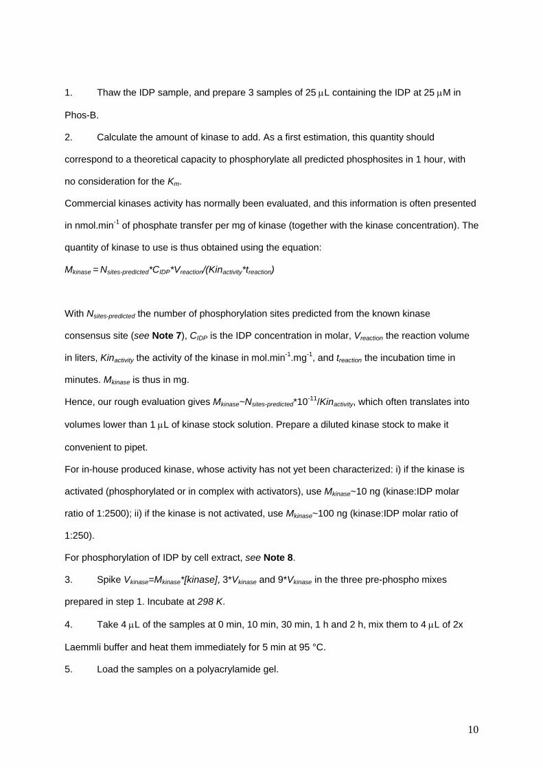
1. Thaw the IDP sample, and prepare 3 samples of 25 L containing the IDP at 25 M in

Phos-B.

2. Calculate the amount of kinase to add. As a first estimation, this quantity should

correspond to a theoretical capacity to phosphorylate all predicted phosphosites in 1 hour, with

no consideration for the Km.

Commercial kinases activity has normally been evaluated, and this information is often presented

in nmol.min-1

of phosphate transfer per mg of kinase (together with the kinase concentration). The

quantity of kinase to use is thus obtained using the equation:

Mkinase = Nsites-predicted*CIDP*Vreaction/(Kinactivity*treaction)

With Nsites-predicted the number of phosphorylation sites predicted from the known kinase

consensus site (see Note 7), CIDP is the IDP concentration in molar, Vreaction the reaction volume

in liters, Kinactivity the activity of the kinase in mol.min-1

.mg-1

, and treaction the incubation time in

minutes. Mkinase is thus in mg.

Hence, our rough evaluation gives Mkinase~Nsites-predicted*10-11

/Kinactivity, which often translates into

volumes lower than 1 L of kinase stock solution. Prepare a diluted kinase stock to make it

convenient to pipet.

For in-house produced kinase, whose activity has not yet been characterized: i) if the kinase is

activated (phosphorylated or in complex with activators), use Mkinase~10 ng (kinase:IDP molar

ratio of 1:2500); ii) if the kinase is not activated, use Mkinase~100 ng (kinase:IDP molar ratio of

1:250).

For phosphorylation of IDP by cell extract, see Note 8.

3. Spike Vkinase=Mkinase*[kinase], 3*Vkinase and 9*Vkinase in the three pre-phospho mixes

prepared in step 1. Incubate at 298 K.

4. Take 4 L of the samples at 0 min, 10 min, 30 min, 1 h and 2 h, mix them to 4 L of 2x

Laemmli buffer and heat them immediately for 5 min at 95 °C.

5. Load the samples on a polyacrylamide gel.

11

6. Run the SDS-PAGE, stain with Coomassie Blue or any other better suited staining

method. Pick the kinase concentration that will permit to distinguish phosphorylation events using

the NMR time resolution, i.e. 15-30 min per time point over 3 to 5 hours (most kinases lose their

activity after a few hours at 25 °C).

7. Buffer conditions can also be evaluated. To this purpose, prepare stock solutions of the

various conditions to test. One may test a range of pH values (pH 7-7.5-8) and of salt

concentrations (50-100-150 mM NaCl). Repeat steps 1-6. If the reaction is much faster at high

pH, adopting the “quenched reaction approach” may be the method of choice to monitor

phosphorylation by NMR. However, if the activity of your kinase is acceptable at pH 7.0, we

recommend running the phosphorylation reaction at this pH. For most kinases, pH 7 corresponds

to an acceptable compromise between kinase activity and decent quality of IDPs’ NMR spectra.

[Fig 2 near here]

3.3. Assignment of NMR Spectra in the Conditions used for Phosphorylation Reactions

To extract residue-specific information, assignment of the IDP’s NMR spectra is a prerequisite.

While phosphorylation reactions will typically be executed at 298 K and pH~7, assignment is

usually performed at conditions favorable for NMR analysis of IDPs, i.e. low temperature (~283 K)

and pH (~6.5), which decrease water/amide proton exchange and consequently maximize S/N.

We will not detail this primary assignment strategy relying on the use of 3-dimensional spectra

establishing connections between spins of backbone nuclei (the most useful ones in the case of

IDPs being HNCO, HN(CA)CO, HNCACB and (H)N(CA)NH).

We describe below the next step that aims at inferring the 1H-

15N crosspeaks assignment in the

conditions used for phosphorylation. It relies on a temperature and pH gradient from the

assignment conditions to the phosphorylation conditions, using DSS as an internal reference. 2D

1H-

15N HSQC or SOFAST-HMQC pulse sequences can be used. SOFAST-HMQC will be better

suited at higher pH and temperature because of its higher S/N efficiency.

1. Record a 2D 1H-

15N HSQC spectrum of the IDP at ~100 M in the pH (pHassign) and

temperature (Tassign) conditions used for prior assignment.

12

2. Record 2D 1H-

15N HSQC or SOFAST-HMQC spectra at the intermediate temperature

(298K-Tassign)/2 and at 298 K.

3. DSS-reference your spectra in both 1H and

15N dimensions (or apply a 10.5 ppb/K shift if

you center the water signal at 4.7 ppm). Then, apply a temperature correction of -7.5 ppb/K in the

proton dimension and -6.5 ppb/K in the nitrogen dimension –do no forget that (15N) is negative.

This will account for the average temperature shifts of random coil amino acids [28], and make

peaks tracking easier.

4. Assign crosspeaks at 298 K by tracing lines through every set of 3 resonances across the

temperature range (see Fig. 3).

5. Apply the same logic for shifting pH progressively from pHassign to pHphosphorylation. Record

2D 1H-

15N HSQC or SOFAST-HMQC spectra at 3 pH values, DSS-reference your spectra (or

apply a 20 ppb/pH unit correction if you center the water peak at 4.7 ppm). In the range of the pH

values considered here, i.e. pH~6.5-7.5, crosspeak frequencies should not shift significantly

except histidine residues and their close neighbors.

[Fig. 3 near here]

3.4. Phosphorylation Monitoring by NMR

A number of IDPs provide poor S/N at pH 7 or higher, due to their high content in hydrophilic

amino acids that show fast water:amide proton exchange (Gly, His, Lys, Arg, Ser, Thr).

Continuous readout at 298 K can thus be greatly hampered by the absence of reliable reporter

crosspeaks. In such situations, it may be more adapted to perform the phosphorylation reaction

on the bench, to remove aliquots and quench the reaction at regular intervals, and to record NMR

spectra of these aliquots later. This “quenched reactions” strategy has an advantage: low pH and

large NMR acquisition times can be used to enhance S/N and resolution. However, the limited

number of time points can hinder the robust fitting and interpretation of phosphorylation kinetics.

In the following, we describe protocols for the continuous readout NMR approach (3.4.1) and for

the discontinuous “quench reaction” approach (3.4.2). To choose between these 2 strategies, you

must evaluate the quality of the 2D 1H-

15N SOFAST-HMQC spectra recorded at pHphosphorylation

and 298 K (see 3.3). If a number of reporter crosspeaks provide S/N ratios above 10, the

13

continuous readout is probably feasible. S/N will depend of course on the IDP concentration and

the tube diameter/volume.

3.4.1 Phosphorylation Monitoring using Continuous NMR Readout

1. Define the final volume of your sample. This ranges from 90 to 475 L depending on the

NMR tube you want to use (see Materials 2.3.4.). Pipetting losses are difficult to avoid, so start

with initial volumes 10-20% higher than the measured ones.

2. Calculate the amount of kinase to add according to 3.2, i.e. the amount leading to

measurable levels of phosphorylation within 2 to 5 hours. The reaction should not be too fast

because the NMR timeframe is on the order of magnitude of 15-30 min in the described

phosphorylation conditions. If you skipped 3.2 and did not test the kinase activity, you may try an

IDP concentration of 50 M, and a kinase:IDP molar ratio of 1:2500 for an activated kinase, or

1:250 for a non-activated kinase.

3. Prepare the pre-phospho mix containing the IDP at 50 M in Phos-B supplemented with

3% D2O and 50 M DSS. Check the pH at room temperature using a micro-pH meter and adjust

it to 7.0 if necessary.

4. Transfer the pre-phospho mix into the NMR tube, insert the tube in an appropriate spinner

and then into the NMR spectrometer equilibrated at 283 K.

5. Tune and match the 1H circuit of the probehead, lock the HOD signal and shim the

sample tube. Determine the 1H 90° pulse.

6. Record 283 K reference 1D 1H spectra and 2D

1H-

15N 2D SOFAST-HMQC spectra using

a FID resolution of ~15 Hz in both 1H and

15N dimensions. This step is recommended to check

the quality of your sample (pH control, ATP/ADP concentrations, IDP degradation) and serves to

measure IDP reference peak intensities. The acquisition time of the 2D spectrum should be

between 30 minutes and 2 hours. Ideally, the S/N of peaks of interest should be 20:1 or more for

an accurate quantification of later phosphorylation advancement.

7. Equilibrate the spectrometer sample temperature at 298 K and re-perform wobbling,

shimming and pulse calibration.

14

8. Record a 298 K reference 1D 1H-spectrum, record two 2D

1H-

15N SOFAST-HMQC

reference spectra using FID resolutions of 15 Hz in 1H dimension and i) 15 Hz and ii) 30 Hz in

15N

dimension. The final acquisition times of the 2D spectra should be about 15 or 30 minutes.

Evaluate the quality of these spectra, try different apodization functions, and pick the parameters

that provide the best compromise between resolution and S/N. These will be used for time-

resolved NMR monitoring of the phosphorylation reaction.

9. Extract the sample from the tube and add the kinase in quantities defined in 3.4.1, step 2.

Mix well by pipetting and load the phosphorylation sample into the same NMR tube.

10. Insert the sample in the magnet, wait 1 minute for temperature equilibration, lock and

shim. Tuning, matching and pulse calibration should not change after addition of the kinase,

unless the kinase stock is very diluted in a very peculiar buffer.

11. Record a 1D 1H-spectrum at 298 K and, then, a series of

1H-

15N 2D SOFAST-HMQC

spectra over 4-12 hours, using the parameters defined in 3.4.8.

12. At the end of the series, shim again and record a 1D 1H spectrum to evaluate the

ADP/ATP ratio (see Note 9).

13. Take back the sample from the tube. At this stage, phosphorylation should not progress

significantly because of the progressive loss of kinase activity. In the case of a heat resistant IDP,

to definitely stop any enzymatic activity, boil the sample at 90 °C for 5 min, centrifuge 5 min at

16,000 xg and recover the supernatant. Avoid boiling IDPs containing Asn-Gly motifs that may

suffer from deamidation. You can alternatively spike EDTA or CyDTA at a final concentration of

15 mM to chelate Mg2+

ions, which will not prevent potential interactions between the IDP and the

kinase and their consequences on IDPs NMR peak intensities.

14. Measure pH and adjust it to the initial value if necessary. ATP, DTT and PI hydrolysis

usually acidify the solution.

15. Fill the NMR tube with the pH-readjusted sample. Insert it in the magnet, set the sample

temperature to 283 K, tune/match, lock and shim. Record 1D 1H spectrum and a 2D SOFAST-

HMQC spectra at 283 K using the same parameters than in 3.4.6. These spectra constitute the

endpoint references.

15

3.4.2 Phosphorylation Monitoring using Quenched Reactions

1. Quenching can be performed using heat inactivation or urea denaturation. Verify that the

studied IDP is resistant to 5 minutes heating at 90 °C. Test it on an aliquot at the concentration

and in the buffer conditions used for the phosphorylation reaction. After 5 minutes, centrifuge 5

minutes at 16,000 xg, separate the supernatant and the eventual aggregated material and

analyze it using SDS-PAGE and NMR. Pay a particular attention to the NMR crosspeaks of Asn

and Gln, whose decreased intensities may reveal deamidation occurring upon heating.

2. If your protein is not heat resistant, you can quench the phosphorylation reaction by

adding phosphorylation reaction buffer supplemented with 10 M urea buffer to the aliquots. The

final urea concentration should be over 4 M. This will require a novel NMR assignment at the final

urea concentration, which can be performed using a urea gradient with the same logic than for

temperature in 3.3. 2D 1H-

15N SOFAST-HMQC spectra of IDPs in urea at pH 7 and 283 K are

usually of high quality.

3. Define the experimental time points (i.e. the number of quenched aliquots) you want to

have, and the final volume and concentration of the measured samples. The corresponding

aliquots can be diluted after being quenched. Such dilution permits a better control of the later pH

adjustment.

4. Calculate the amount of kinase to add according to 3.2 and the time frame you choose. If

you skipped 3.2 and did not test the kinase activity, you may try an IDP concentration of 50 M, a

total reaction time of 5 hours, and an kinase:IDP molar ratio of 1:2500 for an activated kinase, or

1:250 for a non-activated kinase.

5. Prepare the pre-phospho mix containing the IDP at 50 M in Phos-B supplemented with

3% D2O and 50 M DSS. Check the pH at room temperature using a micro-pH meter and adjust

it to pHphosphorylation if necessary.

6. Remove an aliquot and heat it 5 min at 90 °C or dilute it in a urea buffer, according to

3.4.2 step 1. Then, flash-freeze the samples and keep them at -80 °C.

7. Add the kinase in quantities defined in 3.4.2 step 4. Mix well and place it at 298 K in a dry

bath.

16

8. Remove aliquots at the defined time points, and heat them 5 min at 90 °C or dilute them

in a urea buffer. Then, flash-freeze the samples and keep them at -80 °C.

9. After thawing the samples, centrifuge the samples 5 minutes at 16,000 xg if you heated

them. Take the supernatant and complete with the volume of phosphorylation buffer PhosB to

reach the final volume that will be measured by NMR.

10. Adjust the pH to 6.5. Flash freeze the aliquots that you will not measure in the next hours,

keep the other ones on ice.

11. Transfer the sample into the NMR tube, insert the tube in an appropriate spinner and then

into the NMR spectrometer equilibrated at 283 K.

12. Tune and match the 1H circuit of the probehead, lock the HOD signal and shim the

sample tube. Determine the 1H 90° pulse.

13. Record 283 K spectra of every aliquot: a 1D 1H-spectrum and a

1H-

15N 2D SOFAST-

HMQC spectrum using a FID resolution of ~15 Hz in both 1H and

15N dimensions. 1D

1H-spectra

are useful to compare the eventual differences of IDP concentration in the aliquots. They should

thus be recorded with a high S/N. They also permit to check the pH and the ATP/ADP

concentrations. The acquisition time of the 2D spectrum should be between 30 minutes and 2

hours. Ideally, the S/N of peaks of interest should be 20:1 or more for an accurate quantification

of the phosphorylation advancement.

3.5. Analysis of NMR Data

Although a novel assignment of the phosphorylated IDP spectra is not always necessary (see

Note 10), it can be very useful in the case where too many phosphosites generate large number

of spectral changes. We will not detail the assignment method relying on the prior

phosphorylation of a 13

C-15

N labeled IDP and the use of 3-dimensional pulse sequences to

establish sequential connections (see 3.3). A single 3D HNCACB spectrum is often sufficient to

assign the phosphorylated population. We will not elaborate extensively on curve fitting: because

of the progressive kinase loss of activity, the potential IDP degradation, or the competition

between phosphosites, fitting models may often become too complicate to provide consistent

fitted values. In most cases, it is safer to only consider the order of phosphorylation events and

17

their initial rates. Crosspeaks whose intensities vary during the phosphorylation reaction reveal

phosphorylation advancement, and will be called “reporters”. In the following, we describe how to

monitor and quantify the reaction advancement in a residue specific fashion. We will name “non-

phosphopeaks” all crosspeaks found in the reference spectra before phosphorylation, and

“phosphopeaks” those appearing in spectra upon phosphorylation.

1. Fourier transform the spectra recorded at 283 K before and after the phosphorylation

reaction (see 3.4.1 step 6 and 3.4.1 step 15 or 3.4.2 step13) using Topspin or any equivalent

NMR-data processing software. Process these data with an adapted apodization function, and

perform baseline corrections if necessary. The 2D SOFAST-HMQC pulse sequence often

generates distorted baselines in the 15

N-dimension, which alters absolute peak intensities.

2. Load these 2D 283 K-spectra in an NMR data analysis software (i.e. Ccpnmr or Sparky).

Measure intensities of every isolated peak in the reference spectrum (Iref) and after the

phosphorylation reaction (Ifinal).

3. Identify the peaks that faded. Because the corresponding residues are either

phosphorylated or close to phosphorylated residues, these peaks permit identification of the

residues or the segments where phosphorylation reactions occurred. The intensity ratios Ifinal/Iref

of these peaks reveal the final degrees of advancement of these reactions.

4. If you used the “continuous readout approach”, Fourier transform the spectra recorded at

298 K during the phosphorylation reaction and apply baseline corrections if necessary (see

3.5.1). Load these 298 K-spectra in an NMR data analysis software.

5. Measure intensities of every isolated peak in every spectrum, including novel peaks

appearing upon phosphorylation. Pay attention to eventual peak displacements due to pH shifts

in the time series (see Note 11).

6. Plot the evolution curves of every peak using a plot/fit software (Kaleidagraph, Prism,

Gnuplot, ...). If you used the “continuous readout approach”, set the time of the first spectrum to

(tset-up + tacq-spectrum/2), and the later time points to (tset-up+ tacq-spectrum*(n-1/2)). tset-up should be about

5 minutes. Decay of connected non-phosphopeaks, either of phosphosites or of neighboring

residues, should show similar trends.

18

7. Pay attention to the fact that a given residue can sense more than one phosphorylation

reaction, and the decay of its non-phosphopeak may report on more than one phosphorylation

event in its vicinity. Such a situation can be recognized by the appearance of more

phosphopeaks than there were non-phosphopeaks.

8. After identifying non-phosphopeaks that report the same phosphorylation reaction, add

their individual peak intensities at every timepoint (Fig. 1c). This will increase the S/N of the

phosphorylation build-up curves. For every phosphorylation site, evaluate the total intensity It=0 at

time=0 according to the initial slopes of the decay curves. Plot the phosphorylation build-up curve

%phospho(t) = 1-I(t)/It=0.

9. You may try to assign the phosphopeaks. The peaks corresponding to phosphorylated

residues should shift down-field according to the published reference chemical shifts; the

neighboring residues should show weaker peak displacements and remain close to the non-

phosphopeaks. In both cases, peak intensities of phospho- and non-phospho-populations evolve

in a complementary fashion.

10. If no reliable non-phosphopeak reporter can be isolated in the 298 K-spectra, plot the

intensities of the assigned phosphopeaks. Evaluate their intensity Iendpoint at the end of the time

series, according to the last 298 K-spectra (Fig. 1c). Normalize their build-up curve according to

the ratio Ifinal/Iref of non-phosphopeaks measured at 283 K.

11. You can also add build-up curves from related phosphopeak and non-phosphopeaks to

increase S/N. Perform it before intensity normalization and normalize the final build-up curves.

Depending on the shape of the build-up curves there are four possible scenari:

12. If the curve looks like a mono-exponential (Fig. 4a), fit it using %phospho(t)=%phosphot=∞(1-

*exp(-Rphos*t));

13. If the initial IDP concentration is above the Km of a phosphosite, the corresponding decay

curve may look more linear than exponential (Fig. 4b); in this case, fit it using

%phospho(t)=%phosphot=∞(1-(ln(1+(eK-1)*exp(-Rphos*t)))/K), with K=[IDP]/Km;

14. If the curve has an S shape, it may reveal a conditional phosphosite P2 that requires a prior

phosphorylation of a neighboring site P1 (Fig. 4c), which may be fitted using %phosphoP2(t)=1–

[RphosP1*exp(-RphosP2*t)-RphosP2*exp(-RphosP1*t)]/[RphosP1-RphosP2]. In such situation, a set of two P1

19

phosphopeaks should appear, corresponding to P1-noP2 and P1-P2. You can fit %phosphoP1-

noP2(t)= RphosP1/[RphosP1-RphosP2]*[exp(-RphosP2*t)-exp(-RphosP1*t)], and %phosphoP1P2(t)=

%phosphoP2(t).

15. An S shape can also reveal the late phosphorylation of a poor Km, slow phosphosite Pslow

after the early phosphorylation of a faster site Pfast (Fig. 4d). This situation does not provoke

necessarily the apparition of multiple peaks like in 14. Such a build-up curve is fitted

approximately by %phosphoPslow(t)=1-[1-%phosphoPfast)], with

=(VmaxPslow*KMPfast)/(VMaxPFast*KMPslow)<1. Do not pay too much attention to the individual values

obtained upon fitting, but consider only the initial rates calculated from fitted parameters (see

Note 12).

[Figure 4 near here]

4. Notes

1. The lowest IDP concentration to obtain sufficient S/N is about 12.5 M in most cases.

Phosphorylation monitoring by NMR is however often performed at much higher concentrations in

the literature, sometimes at several hundreds of micromolar. Importantly, at high IDP

concentrations, kinases are likely to steadily phosphorylate non-specific sites with very high Km.

NMR concentrations may thus generate questionable results if this aspect is neglected. Kms of

kinases for their cognate targets span a wide range of values, from 1 to 100 M, while kcat values

can vary between 0.01 and 100 s-1

(we did not find an article providing statistics, these are

numbers based on long-term experience, you can try https://www.brenda-enzymes.org/). We

highly recommend to measure kinetics at a given concentration and at either half or twice this

concentration. The measured initial rates (in mol.s-1

) will reveal whether the used concentrations

are below or above the Km of every detected phosphosite, and whether some sites emerge only

because of high concentrations. There are three possibilities: i) if the molar phosphorylation rate

is proportional to the substrate concentration, we are well below the phosphosite Km, which may

20

be odd at concentrations above 100 M for example; ii) if it is the same at both concentrations,

we are an order of magnitude above the Km, which may call for running the phosphorylation

reaction at lower concentration; iii) intermediate situations mean that we are at a concentration in

the order of magnitude of the Km. Of course, it is ideally preferable to determine kcat and Km more

precisely by measuring initial rates at multiple concentrations following the Michaelis-Menten

approach.

2. Cysteine reduction can usually be obtained by supplementing the lysis buffer with 10 mM DTT

(final concentration), and by spiking 5 mM DTT (final concentration) in protein samples after

every purification step. Avoid -mercaptoethanol: it is a poor reducing agent and it easily forms

mixed disulfides with cysteines. TCEP is advantageous in many regards, but its notorious stability

is affected by the presence of phosphate and EGTA [24, 31], it requires pH adjustment after

solubilization, and it may cleave progressively the protein backbone near cysteines [32].

3. IDPs are generally very well expressed in E. coli strains optimized for protein production.

Bacteria are grown in minimum media containing 15

NH4Cl and 13

C-glucose as sole sources of

nitrogen and carbon, respectively. Recipes can be found at

https://www.embl.de/pepcore/pepcore_services/protein_expression/ecoli/n15/ or in [29]. IDPs can

sometimes be obtained in inclusion bodies: in such situation, they can be first purified in urea

using a Histidine tag, before being transferred in a non-denaturant buffer using SEC.

4. High buffering capacity is important because ATP and DTT hydrolysis release protons and can

provoke deleterious pH variations. A careful control of the pH is indeed essential to generate

NMR data of high quality: crosspeak intensities of IDPs amide functions can vary up to ~10% for

a pH shift of 0.1 at pH 7 and 298 K (This is due to the pH-dependency of water/amide proton

exchange [37], hence to the residence time of the detected amide protons). Because we

calculate phospho and non-phospho populations based on NMR crosspeak intensities, pH

variations can thus bias this quantification.

21

5. Recombinant expression in insect or mammalian cells may produce prephosphorylated protein

samples. This may be detected using the Pro-Q Diamond Phosphoprotein Gel Stain kit, Phos-

Tag SDS-PAGE [30], Mass Spectrometry or Western blot with an antibody directed against

phosphoSer/Thr. It can also be detected using 2D 1H-

15N NMR spectroscopy, given the

recognizable chemical shifts adopted by phosphorSer/Thr residues [16, 21]. Tyrosine

phosphorylation can be nailed using 1H-

13C NMR spectroscopy because of the C chemical shifts

perturbation [21]. If prephosphorylation is ascertained, a phosphatase treatment may be carried

out during the purification.

6. Adding 10% glycerol to the reaction mix often improves S/N and decreases the pH-

dependency of NMR crosspeak intensities. It provokes chemical shift perturbations, which may

be large enough to force a supplementary assignment step. This can be carried out similarly to

what has been described for temperature-dependent assignment in 3.3.

7. Kinases achieve substrate specificity in many ways [33]. Several servers exist predicting

phosphorylation sites and their associated kinases. They rely mostly on kinase consensus site

analysis, reported detection and existing annotation or interaction networks in databases [34, 35].

An extensive list of methods is available in [36]. A simple consensus site analysis can be

obtained using http://www.cbs.dtu.dk/services/NetPhos/, lists of detected phosphorylation sites is

available on https://www.phosphosite.org/.

8. Monitoring IDP phosphorylation in cell extracts is a challenging task. Which cell line? Which

lysis conditions? In exponential growth phase, or after cell-cycle arrest and at which stage?

Whole cell extract or separation of specific cell compartment? These parameters will generate

very different extracts with highly variable phosphorylation activities. For this reason, we thought

it was difficult to provide a generic protocol, and we prefer to refer to guidelines published

previously [17]. Producing active extracts requires fast manipulation of the cellular material. Lysis

buffers should of course be non-denaturing and contain large concentrations of protease and

phosphatase inhibitors. ATP hydrolysis is usually intense because of the combined activity of

22

several cellular kinases. Extract concentration should be high (1-10 mg.mL-1

). The experimental

timeframe is usually about one hour, although it can be difficult to establish: early phosphorylation

can be rapidly compensated by dephosphorylation activity of cellular phosphatases, which often

take over anyway after ATP exhaustion. We finally warn the reader that interpretation of

phosphorylation kinetics in cell extracts should be cautious: native cellular organization and

colocalization is essential in cell signaling, and is lost in cell extracts; the IDP of interest may

interact with enzymes that it would not meet in a real cell, and kinase or phosphatase activity

regulation may quickly degenerate.

9. Kinases affinity for ATP is in the range of 10 to 100 M, and up to the millimolar range in a

minority of cases [38]. Affinity for ADP is in the same range and very well correlated to that of

ATP [38]. Hence, a large excess of ATP is recommended for monitoring phosphorylation

reactions in vitro to avoid strong inhibition by growing concentrations of ADP. Moreover, we

observed in most cases that kinases hydrolyze more ATP molecules than they transfer

phosphate moieties to their substrate. We recommend to measure 1D 1H spectra before and after

the reaction to evaluate the ratio ATP/ADP (Fig. 5), which may help in interpreting the

progressive loss of kinase activity.

[Figure 5 near here]

10. The most prominent chemical shift changes occur for phosphorylated residues. Their

crosspeaks show strong downfield-shifts in 1H-

15N 2D spectra upon phosphorylation: due to a

hydrogen bond between the new side-chain phosphate and the backbone amide function, their

1H resonances move to 8.5-9.5 ppm, which is out of the regular spectral window (7.5-8.5 ppm) for

disordered peptides [16, 21]. However, the corresponding peaks move upfield when pH acidifies,

and their absolute intensities are also pH dependent. In surprising cases, crosspeaks in this

“phospho-region” of 8.5-9.5 ppm can reveal a H-bond between the side-chain phosphate of a

phosphorylated residue and the amide proton of a non-phosphorylated residue [39]. 13

C and

13C chemical shifts provide unambiguous information on the nature of these

1H-

15N crosspeaks

23

(phosphoSer/Thr, or neighboring non-modified residue establishing a H-bond with a phosphate).

Recording a 3D HNCACB spectrum is thus often of good help in the analysis of the NMR data,

which requires a 13

C/15

N-labeled IDP.

11. Because phosphoSer and phosphoThr have pKa values of about 6 and 6.5, respectively [21,

40], their protonation state vary with the potential pH evolution during the phosphorylation

reaction, as evoked in note 3. This provokes chemical shift perturbations of the phosphorylated

residues and of their neighbors. Hence, it is important to verify that intensities are measured at

the peak centers in every spectrum.

12. Complex mechanisms emerging from multiple phosphorylation sites can take place.

Assigning all peaks when multiple neighbor phosphosites evolve concomitantly can be tedious.

Fitting evolution curves in such situations, or in the case of large Km differences between

phosphosites is always possible. Equations that can be used to fit complex phosphorylation

schemes have been described extensively earlier [17]. However, the fitted parameters should be

used cautiously: little differences in the range of the S/N (and thus inside the error bars) for a

couple of early points can provoke large differences in the fitted values; moreover, the

progressive loss of kinase activity during the hours-long reaction is very difficult to evaluate.

Hence, we argue that one should limit the interpretation of the recorded kinetics to i) the ranking

between phosphorylation sites and ii) the initial rates of phosphorylation.

Acknowledgement

This work was supported by CNRS, CEA, University Paris South and ENS Paris-Saclay, by the

French Infrastructure for Integrated Structural Biology

(https://www.structuralbiology.eu/networks/FRISBI, grant number ANR-10-INSB-05-01, Acronym

FRISBI) and by the French National Research Agency (ANR; research grant ANR-14-ACHN-

0015). We thank the protein production facility of the Institut Curie for providing the purified

kinase Plk1.

24

References

1. Hornbeck PV, Kornhauser JM, Latham V, et al (2019) 15 years of PhosphoSitePlus®:

integrating post-translationally modified sites, disease variants and isoforms. Nucleic Acids

Res 47:D433–D441. doi: 10.1093/nar/gky1159

2. Huang K-Y, Lee T-Y, Kao H-J, et al (2019) dbPTM in 2019: exploring disease association

and cross-talk of post-translational modifications. Nucleic Acids Res 47:D298–D308. doi:

10.1093/nar/gky1074

3. Vlastaridis P, Kyriakidou P, Chaliotis A, et al (2017) Estimating the total number of

phosphoproteins and phosphorylation sites in eukaryotic proteomes. Gigascience 6:1–11.

doi: 10.1093/gigascience/giw015

4. Yu K, Zhang Q, Liu Z, et al (2019) qPhos: a database of protein phosphorylation dynamics

in humans. Nucleic Acids Res 47:D451–D458. doi: 10.1093/nar/gky1052

5. Wright PE, Dyson HJ (2015) Intrinsically disordered proteins in cellular signalling and

regulation. Nat Rev Mol Cell Biol 16:18–29. doi: 10.1038/nrm3920

6. Schweiger R, Linial M (2010) Cooperativity within proximal phosphorylation sites is

revealed from large-scale proteomics data. Biol Direct 5:6. doi: 10.1186/1745-6150-5-6

7. Sharma K, D’Souza RCJ, Tyanova S, et al (2014) Ultradeep Human Phosphoproteome

Reveals a Distinct Regulatory Nature of Tyr and Ser/Thr-Based Signaling. Cell Rep

8:1583–1594. doi: 10.1016/j.celrep.2014.07.036

8. Theillet F-X, Binolfi A, Frembgen-Kesner T, et al (2014) Physicochemical properties of

cells and their effects on intrinsically disordered proteins (IDPs). Chem Rev 114:6661–

6714. doi: 10.1021/cr400695p

9. Landry CR, Freschi L, Zarin T, Moses AM (2014) Turnover of protein phosphorylation

25

evolving under stabilizing selection. Front Genet 5:245. doi: 10.3389/fgene.2014.00245

10. Nishi H, Shaytan A, Panchenko AR (2014) Physicochemical mechanisms of protein

regulation by phosphorylation. Front Genet 5:270. doi: 10.3389/fgene.2014.00270

11. Levy ED, Michnick SW, Landry CR (2012) Protein abundance is key to distinguish

promiscuous from functional phosphorylation based on evolutionary information. Phil

Trans R Soc B 367:2594–2606. doi: 10.1098/rstb.2012.0078

12. Wu R, Haas W, Dephoure N, et al (2011) A large-scale method to measure absolute

protein phosphorylation stoichiometries. Nat Meth 8:677–683. doi: 10.1038/nmeth.1636

13. Kanshin E, Pascariu M, Tyers M, et al (2018) Combined Enrichment/Enzymatic Approach

To Study Tightly Clustered Multisite Phosphorylation on Ser-Rich Domains. J Proteome

Res 17:3050–3060. doi: 10.1021/acs.jproteome.8b00205

14. Riley NM, Coon JJ (2016) Phosphoproteomics in the Age of Rapid and Deep Proteome

Profiling. Anal Chem 88:74–94. doi: 10.1021/acs.analchem.5b04123

15. Humphrey SJ, Karayel O, James DE, Mann M (2018) High-throughput and high-sensitivity

phosphoproteomics with the EasyPhos platform. Nat Protoc 13:1897–1916. doi:

10.1038/s41596-018-0014-9

16. Theillet F-X, Smet-Nocca C, Liokatis S, et al (2012) Cell signaling, post-translational

protein modifications and NMR spectroscopy. J Biomol NMR 54:217–236. doi:

10.1007/s10858-012-9674-x

17. Theillet F-X, Rose HM, Liokatis S, et al (2013) Site-specific NMR mapping and time-

resolved monitoring of serine and threonine phosphorylation in reconstituted kinase

reactions and mammalian cell extracts. Nat Protoc 8:1416–1432. doi:

10.1038/nprot.2013.083

18. Smith MJ, Marshall CB, Theillet F-X, et al (2015) Real-time NMR monitoring of biological

activities in complex physiological environments. Curr Opin Struct Biol 32:39–47. doi:

26

10.1016/j.sbi.2015.02.003

19. Cordier F, Chaffotte A, Terrien E, et al (2012) Ordered phosphorylation events in two

independent cascades of the PTEN C-tail revealed by NMR. J Am Chem Soc 134:20533–

20543. doi: 10.1021/ja310214g

20. Mylona A, Theillet F-X, Foster C, et al (2016) Opposing effects of Elk-1 multisite

phosphorylation shape its response to ERK activation. Science 354:233–237. doi:

10.1126/science.aad1872

21. Bienkiewicz EA, Lumb KJ (1999) Random-coil chemical shifts of phosphorylated amino

acids. J Biomol NMR 15:203–206.

22. Liokatis S, Stützer A, Elsässer SJ, et al (2012) Phosphorylation of histone H3 Ser10

establishes a hierarchy for subsequent intramolecular modification events. Nat Struct Mol

Biol 19:819–823. doi: 10.1038/nsmb.2310

23. Hendus-Altenburger R, Pedraz-Cuesta E, Olesen CW, et al (2016) The human Na(+)/H(+)

exchanger 1 is a membrane scaffold protein for extracellular signal-regulated kinase 2.

BMC Biol 14:31. doi: 10.1186/s12915-016-0252-7

24. Getz EB, Xiao M, Chakrabarty T, et al (1999) A comparison between the sulfhydryl

reductants tris(2-carboxyethyl)phosphine and dithiothreitol for use in protein biochemistry.

Anal Biochem 273:73–80. doi: 10.1006/abio.1999.4203

25. Schanda P, Kupče Ē, Brutscher B (2005) SOFAST-HMQC Experiments for Recording

Two-dimensional Deteronuclear Correlation Spectra of Proteins within a Few Seconds. J

Biomol NMR 33:199–211. doi: 10.1007/s10858-005-4425-x

26. Theillet F-X, Binolfi A, Liokatis S, et al (2011) Paramagnetic relaxation enhancement to

improve sensitivity of fast NMR methods: application to intrinsically disordered proteins. J

Biomol NMR 51:487–495. doi: 10.1007/s10858-011-9577-2

27. Lee C-R, Park Y-H, Kim Y-R, et al (2013) Phosphorylation-Dependent Mobility Shift of

27

Proteins on SDS-PAGE is Due to Decreased Binding of SDS. Bull Korean Chem Soc

34:2063–2066. doi: 10.5012/bkcs.2013.34.7.2063

28. Kjaergaard M, Brander S, Poulsen FM (2011) Random coil chemical shift for intrinsically

disordered proteins: effects of temperature and pH. J Biomol NMR 49:139–149. doi:

10.1007/s10858-011-9472-x

29. Azatian SB, Kaur N, Latham MP (2019) Increasing the buffering capacity of minimal media

leads to higher protein yield. J Biomol NMR 73:11–17. doi: 10.1007/s10858-018-00222-4

30. Kinoshita E, Kinoshita-Kikuta E, Koike T (2009) Separation and detection of large

phosphoproteins using Phos-tag SDS-PAGE. Nat Protoc 4:1513–1521. doi:

10.1038/nprot.2009.154

31. Hansen RE, Winther JR (2009) An introduction to methods for analyzing thiols and

disulfides: Reactions, reagents, and practical considerations. Anal Biochem 394:147–158.

doi: 10.1016/j.ab.2009.07.051

32. Liu P, O'Mara BW, Warrack BM, et al (2010) A tris (2-carboxyethyl) phosphine (TCEP)

related cleavage on cysteine-containing proteins. J Am Soc Mass Spectrom 21:837–844.

doi: 10.1016/j.jasms.2010.01.016

33. Miller CJ, Turk BE (2018) Homing in: Mechanisms of Substrate Targeting by Protein

Kinases. Trends Biochem Sci 43:380–394. doi: 10.1016/j.tibs.2018.02.009

34. Horn H, Schoof EM, Kim J, et al (2014) KinomeXplorer: an integrated platform for kinome

biology studies. Nat Meth 11:603–604. doi: 10.1038/nmeth.2968

35. Patrick R, Horin C, Kobe B, et al (2016) Prediction of kinase-specific phosphorylation sites

through an integrative model of protein context and sequence. BBA - Proteins and

Proteomics 1864:1599–1608. doi: 10.1016/j.bbapap.2016.08.001

36. Palmeri A, Ferrè F, Helmer-Citterich M (2014) Exploiting holistic approaches to model

specificity in protein phosphorylation. Front Genet 5:315. doi: 10.3389/fgene.2014.00315

28

37. Bai Y, Milne JS, Mayne L, Englander SW (1993) Primary structure effects on peptide

group hydrogen exchange. Proteins 17:75–86. doi: 10.1002/prot.340170110

38. Becher I, Savitski MM, Savitski MF, et al (2013) Affinity profiling of the cellular kinome for

the nucleotide cofactors ATP, ADP, and GTP. ACS Chem Biol 8:599–607. doi:

10.1021/cb3005879

39. Smet-Nocca C, Launay H, Wieruszeski J-M, et al (2013) Unraveling a phosphorylation

event in a folded protein by NMR spectroscopy: phosphorylation of the Pin1 WW domain

by PKA. J Biomol NMR 55:323–337. doi: 10.1007/s10858-013-9716-z

40. Platzer G, Okon M, McIntosh LP (2014) pH-dependent random coil 1H, 13C, and 15N

chemical shifts of the ionizable amino acids: a guide for protein pK a measurements. J

Biomol NMR 60:109–129. doi: 10.1007/s10858-014-9862-y

Figure Captions

Fig. 1: NMR analysis of BRCA2(aa48-218) phosphorylation by Plk1 ([BRCA2]=50 M, [Plk1]=200

nM, spectra recorded at 700 MHz). a) Overlay of 1H-

15N 2D HSQC spectra recorded at 283 K

before (reference, black) and after the phosphorylation reaction (tfinal, red). Arrows highlight NMR

chemical shift perturbations upon phosphorylation. The two phosphosites S193 and T207

crosspeaks show large perturbation; their neighbor residues D189, S193, S195 and L198, T203

and V211 also shift and can be used as phosphorylation reporters. Measuring the crosspeak

intensities of the non-modified species (called later “non-phosphopeaks”) in the two 283 K

spectra provides Ifinal/Iref ratios, which later permit normalization of the phosphorylation build-up

curves. b) Depiction of three time-points in the time series of 2D 1H-

15N SOFAST-HMQC spectra

recorded at 298 K during the reaction (grey spectra). We superimposed them on the reference

spectrum at t=0 (black spectrum). Close-up views show the evolution of 3 couples of “non-

phosphopeaks” and “phosphopeaks”: A199 crosspeaks (orange) report on S193 phosphorylation,

29

while T207 (magenta) and V211 (blue) crosspeaks report on T207 phosphorylation. The non-

phosphoT207 peak partially overlaps with other resonances, and is thus a reporter of poor

quality. c) Treatment of peak intensities from raw data, to normalized intensities and

interpretation in %phosphorylation. The value Intt=0 of a non-phosphopeak is obtained from the

tangent at t=0 of a non-phosphopeak evolution curve, and can then be used for normalizing this

evolution. Build-up curves of phosphopeaks are normalized by intensity ratios measured at 283 K

Ifinal/Iref (see 3.5). To make the graphs clearer, we show only A199 crosspeaks evolution as a

reporter of S193 phosphorylation; S193, S195 and L198 crosspeaks can also be used, see a).

Similarly, T203 crosspeaks can be used as reporters of T207 phosphorylation. Phosphorylation

build-up curves are preferably obtained from non-phosphopeaks decay analysis. They can be

normalized easily using the reference intensities at 0% phosphorylation; at the opposite, because

a phosphorylation reaction rarely goes to completion, the reference intensities of phosphopeaks

at 100% phosphorylation can be difficult to determine.

Fig. 2. SDS-PAGE analysis of the phosphorylation kinetics of a BRCA2 fragment presenting 5

phosphosites. Phosphorylation of the wild-type fragment and a mutant fragment were evaluated

at t0, t10min, t30min and t2hrs. This gel exemplifies the typical phosphorylation shifts provoked by

successive phosphorylation events. Although it is no fully characterized, it appears that SDS

binds less to phosphoproteins, which slows down electrophoretic migration [27]. Peptides

carrying a high net negative charge (~15 or more) do not shift as well upon phosphorylation.

(15% polyacrylamide gel stained with Coomassie blue, lane X shows a default in gel loading).

Fig. 3. Temperature gradient from assignment conditions (283 K) to phosphorylation conditions

(298 K) allows fast 1HN and

15N assignment at 298 K. 2D

1H-

15N SOFAST-HMQC spectra of

BRCA2(aa48-218) were recorded at 283 K, 290 K and 298 K, and spectral referencing were

temperature-corrected according to the rule presented in 3.3.3. All spectra are shown at the same

contour level. A number of crosspeaks fade away at higher temperature. This is typical of IDPs

NMR spectra. The spectra were acquired at pH 7.0 and 700 MHz.

30

Fig. 4: Theoretical phosphorylation build-up curves. a) Build-up curves in the situation where the

phosphorylation target is at a concentration well below its Km. b) Build-up curves in the situation

where the phosphorylation target is at concentrations above its Km (black: [substrate]<<Km;

brown: [substrate]=2*Km; orange: [substrate]=5*Km; red: [substrate]=10*Km). c) Build-up curves

in the situation where the substrate carries 2 phosphorylation sites and the 2nd

phosphosites (in

blue) is phosphorylated only once the 1st phosphosite (in red) has been modified. d) Build-up

curves in the situation where the substrate carries 2 phosphorylation sites with

Km(P1)=10*Km(P2) (P1 is in red, P2 in blue).

Fig. 5: NMR analysis of the ATP/ADP concentrations. Upper panel: Overlay of 1D 1H spectra of

pure ATP (blue) and ADP (red) showing the purine 1H35 resonances. Lower panel: 1D

1H

spectrum of BRCA2(aa48-218) at 50 M at the end of the phosphorylation reaction by Plk1. The

close-up view shows the ATP and ADP 1H35 signals allowing their quantification. All spectra were

recorded in the phosphorylation buffer (50 mM Hepes, 100 mM NaCl, pH 7.0, 4 mM DTT, 1x

EDTA-free protease inhibitors, 4 mM ATP, 10 mM MgCl2) at 283 K and at 700 MHz. ATP and

ADP 1H35 chemical shifts depend on pH and on the presence of Mg

2+ (~0.03 ppm).