Multinational Production and Labor Share*

Daisuke Adachi† Yukiko U. Saito‡

December 14, 2020

[Click here for the latest version]

Abstract

We investigate the impact of multinational enterprises (MNEs) on the source-country

labor share. Our model shows that source-country factor demand elasticities with re-

spect to foreign factor prices affect aggregate labor share. To identify these elastici-

ties, we develop an estimator that leverages a foreign factor-productivity shock. We

apply this estimator to a unique natural experiment: the 2011 Thailand Floods, which

negatively impacted the foreign operation of Japanese MNEs. We employ a uniquely

combined Japanese firm- and plant-level microdata and find that the Floods decreased

fixed assets in Japan more than employment, suggesting that foreign factor productivity

growth reduces Japan’s labor share.

Keywords: Multinational enterprise; Labor share; Bias in technological change; Elas-

ticity of factor substitution; Natural experiment; The 2011 Thailand Flood.

JEL codes: F23, E25, J23, F21, F66

1 Introduction

A growing body of evidence suggests that in recent decades, the labor share of national

income has decreased in several developed countries (Karabarbounis and Neiman, 2013),

raising concerns both for policymakers and economists. For policymakers, the decrease

*We appreciate helpful comments by Pol Antras, Costas Arkolakis, Dominick Bartelme, Kirill Borusyak,Bill Brainard, Lorenzo Caliendo, Cheng Chen, Rafael Dix-Carneiro, Michal Fabinger, Pablo Fajgelbaum, AnaCecilia Fieler, Teresa Fort, Sharat Ganapati, Kailin Gao, Jay Junsik Hyun, Sam Kortum, Giovanni Maggi, Ken-taro Nakajima, Guillermo Noguera, Nitya Pandalai-Nayar, Micheal Peters, Peter Schott, Daisy Sun, Yuta Taka-hashi, Lucas Zavala, Ray Zhang, and seminar participants at Colorado Boulder, Columbia, IU Bloomington,NYU, RIETI, SNU, and Yale. We acknowledge data provision from the Research Institute of Economy, Tradeand Industry (RIETI) and Costas Arkolakis. Saito acknowledges the financial support from the RIETI project“Dynamics of Inter-organizational Network and Firm Lifecycle” and the Japan Society for the Promotion ofScience (#18H00859 and #20K20511). We also thank Takashi Iino for outstanding research assistance and PhilipC. MacLellan for editorial assistance. All remaining errors are ours.

†Yale University and RIETI. daisuke.adachi@yale.edu.‡Waseda University and RIETI, SF. saito-yukiko@waseda.jp.

1

might be interpreted as an increase in income inequality between capital holders and la-

borers. For economists, it challenges one of the stylized facts of growth models (Kaldor,

1961).

The broad question of the current paper is what drove the decrease in the labor share.

Several potential explanations have been proposed in the literature, including the role of

bias in technological change (Oberfield and Raval, 2014), for if changes in productivity aug-

ment capital more than labor, then the total payment to labor will decrease relative to cap-

ital. Although this is a theoretically coherent and straightforward explanation, there are

several potential mechanisms behind such factor-specific augmentation. For example, the

production processes are fragmenting across the world (Johnson and Noguera, 2012, 2017).

If international direct investment and employment of foreign labor by multinational enter-

prises (MNEs) complements capital in the source country, there can be a relative increase in

the demand for capital relative to labor. In this paper, we formalize this idea and ask if and

to what extent it may explain the labor share trend in the source country of foreign direct

investment (FDI).

This surge in MNE international factor employment has been brought about by a wide

range of changes in the economic environment, including technological change, policy and

institutional reform, and growth of developing economies. For example, better global com-

munication technologies, removal of political barriers regarding international direct invest-

ment and employment of foreign labor, and increasing demand by external economies all

may have increased the availability and productivity of foreign factors. We take these events

as exogenous augmentations of foreign factors for MNEs and study the effects on the labor

share of the source country.

As first-pass evidence, Figure 1 shows a significant negative ralationship between the

change in net MNE sales and labor share among countries. Although we do not suggest that

the correlation is causal, this negative relationship is consistent with the idea that the out-

ward activities of MNEs complement capital demand more than labor in the source country.

To formally answer the question if and how much foreign factor augmentation decreased

the labor share in the source country, we proceed in three steps. First, we develop a general

equilibrium model that features heterogeneous and non-parametric production functions

that include the employment and exogenous augmentations of the foreign factors. In the

model, the factor market-clearing wages are the key endogenous variables determining la-

bor share, and we show that to the first order, the elasticity structure of factor demand is

critical to the the direction and size of the change in labor share. This first order approxima-

tion is robust across several existing models of multinational production and many factors,

including models of offshoring (e.g., Feenstra and Hanson, 1997) and multinational pro-

duction with export platforms (e.g., Arkolakis et al., 2017). We then show how the key

2

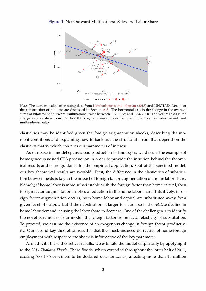
Figure 1: Net Outward Multinational Sales and Labor Share

Note: The authors’ calculation using data from Karabarbounis and Neiman (2013) and UNCTAD. Details ofthe construction of the data are discussed in Section A.5. The horizontal axis is the change in the averagesums of bilateral net outward multinational sales between 1991-1995 and 1996-2000. The vertical axis is thechange in labor share from 1991 to 2000. Singapore was dropped because it has an outlier value for outwardmultinational sales.

elasticities may be identified given the foreign augmentation shocks, describing the mo-

ment conditions and explaining how to back out the structural errors that depend on the

elasticity matrix which contains our parameters of interest.

As our baseline model spans broad production technologies, we discuss the example of

homogeneous nested CES production in order to provide the intuition behind the theoret-

ical results and some guidance for the empirical application. Out of the specified model,

our key theoretical results are twofold. First, the difference in the elasticities of substitu-

tion between nests is key to the impact of foreign factor augmentation on home labor share.

Namely, if home labor is more substitutable with the foreign factor than home capital, then

foreign factor augmentation implies a reduction in the home labor share. Intuitively, if for-

eign factor augmentation occurs, both home labor and capital are substituted away for a

given level of output. But if the substitution is larger for labor, so is the relative decline in

home labor demand, causing the labor share to decrease. One of the challenges is to identify

the novel parameter of our model, the foreign factor-home factor elasticity of substitution.

To proceed, we assume the existence of an exogenous change in foreign factor productiv-

ity. Our second key theoretical result is that the shock-induced derivative of home-foreign

employment with respect to the shock is informative of the key parameter.

Armed with these theoretical results, we estimate the model empirically by applying it

to the 2011 Thailand Floods. These floods, which extended throughout the latter half of 2011,

causing 65 of 76 provinces to be declared disaster zones, affecting more than 13 million

3

people, and creating an estimated 1,425 trillion baht (USD 46.5 billion) in economic losses

(World Bank), were a severe negative foreign factor productivity shock to Japanese MNEs

operating in the flooded regions.

To study this unique event, we employ and combine firm- and establishment-level mi-

crodata sourced from the Basic Survey on Japanese Business Structure and Activities (BSJBSA),

the Basic Survey on Overseas Business Activities (BSOBA), and the Orbis database from Bureau

van Dijk (Orbis BvD). First, we calibrate the capital-labor substitutability by the first order

condition and a shift-share-type instrumental variable (Raval, 2019). Consistent with the

previous literature, we find that capital-labor are gross complements. Second, by regressing

the log-home employment on the log-foreign employment (with the instrumental variable

relating the intensity of the flood damage) and a firm-level fixed effect, we obtain a two-

stage least squares estimate which indicates that home labor and foreign labor are gross

substitutes, in keeping with our theory. This result is based on our homogeneous nested

CES specification.

Given the home labor-foreign labor substitutability implied by our estimate, we find that

foreign factor augmentation (from the perspective of Japan) did contribute to a decrease in

labor share in Japan. We thus have shown that foreign factor augmentation decreases home

labor share. To quantify this, we exploit the nested CES specification to back out the aggre-

gate evolution of foreign factor-augmenting productivities. Applying our implied elastic-

ities of substitution, we find that foreign factor augmentation alone explains 59 percent of

the decrease in Japan’s labor share between 1995 and 2007.

We also derive an elasticity estimate from a more general production function based on

the method of moments. As in the nested CES case, the result shows that foreign factor

augmentation increases the relative demand for capital, which implies that the relative labor

wage decreases, as does the labor share.

The paper is structured as follows. After discussing the related literature below, Sec-

tion 2 provides some of the motivating facts about labor share and MNEs. Section 3 then

provides the conceptual framework modeling labor share and foreign factor augmentation,

presenting both a general foreign factor demand model and a nested CES specification. Sec-

tion 4 discusses the empirical setting, data, specification and reduced-form estimates, while

Section 5 shows the derived structural parameters and estimation under both the general

and nested CES models. Section 6 concludes the paper.

1.1 Related Literature

This paper relates to two strands of literature: research concerning the recent decreasing la-

bor share (or increasing capital share) of production, and studies on MNEs and their impact

4

on the source country’s labor market.

1.1.1 Changing Factor Shares

Seminal research on changing factor shares that empirically finds a decreasing labor share

includes Elsby et al. (2013) in the U.S and Karabarbounis and Neiman (2013), whose com-

parable cross-country data show a declining labor share in many developed countries in

particular, which Piketty and Zucman (2014) have suggested leads to expanding within-

country income inequalities. However, there are several conceptual qualifications and labor

share measurement issues that raise concerns about these empirical findings. For instance,

Rognlie (2016, 2018); Bridgman (2018) stress that the treatment of capital depreciation and

the self-employee income allotment to each factor entails strong assumptions. Making a

different argument, Koh et al. (2018) claim that the decline in the labor share in the U.S

is attributable mainly to the capitalization of intellectual property, while Cette et al. (2019)

discuss a similar effect regarding the accounting of real estate income. In our view, even af-

ter taking these qualifications into account, Japan’s labor share between 1995 and 2007 still

decreased, as discussed further in Section A.2.

There are several possibilities suggested in the literature as to why the labor share is

decreasing, including bias in technological change. For instance, Oberfield and Raval (2014)

emphasize the role of “technology, broadly defined, including automation and offshoring,

rather than mechanisms that work solely through factor prices”, and Elsby et al. (2013)

conclude that the offshoring of labor-intensive activities within the supply chain is “the

leading potential explanation of the decline in the U.S. labor share over the past 25 years.”

On the technology side, automation technology may have contributed to the labor share

decrease, as reviewed in Acemoglu and Restrepo (2019) for the example of industrial robots.

To these, we add globalization as a partial explanation, particularly in our context of Japan

from 1995-2007. We offer evidence based on a particular mechanism that features the role

of MNEs, providing a novel identification strategy and empirical evidence from the 2011

Thailand Floods.1

An increase in market power (and thus profit) by dominant corporations has also been

proposed as a reason for decreasing labor share, as market power can emerge both in the

goods market (Autor et al., 2017a,b; Barkai, 2017; De Loecker and Eeckhout, 2017) and in the

labor market (Gouin-Bonenfant et al., 2018; Berger et al., 2019).2 Although market power is

not our main focus, we explore its potential role to help validate our mechanism. Apply-

ing the method of De Loecker and Eeckhout (2017) to our Japanese data, we find that the1Other potential explanations for declining labor share include lower capital and increasing risk premiums,

as discussed in detail in Section A.4.2Berger et al. (2019), however, argue that labor market concentration contributed in the opposite direction,

if at all, as the U.S. local labor market concentration has been decreasing since the 1970s.

5

markup did not increase as much in Japan as in the U.S.

Our contribution to this literature is adding multinational enterprises (MNEs) to the dis-

cussion of potential reasons for the observed decrease in labor share. Among this growing

literature, we regard our work to be closest to Oberfield and Raval (2014) who, as mentioned

above, emphasize the role of biased technological change in the production function as op-

posed to the factor-price story of Karabarbounis and Neiman (2013). For this purpose, they

employ plant-level microdata in the U.S. and estimate the capital-labor substitution elastic-

ity by estimating the first order condition for factor demand with a Bartik-type instrument.

They find that since the 1970s, the aggregate capital-labor elasticity has been constant at

around 0.7, which indicates that capital and labor are indeed gross complements, while a

capital cost decline like that emphasized by Karabarbounis and Neiman (2013) would im-

ply an increasing labor share. Our analysis draws upon and extends Oberfield and Raval

(2014), first applying their method of estimating capital-labor elasticity to firm- and plant-

level data in Japan to confirm that the elasticity is below one. We depart from their analysis

to the extent that we explicitly incorporate the foreign factor employment of home firms in

our model in order to consider the effect of foreign factor augmentation on the home labor

share. Section 3.1 explains how our production function nests that of Oberfield and Raval

(2014).

1.1.2 Labor Market Impact of MNEs

This paper also relates to a second line of research that examines the impact of foreign pro-

duction on the source country’s labor market (Desai et al., 2009; Muendler and Becker, 2010;

Harrison and McMillan, 2011; Ebenstein et al., 2014; Boehm et al., 2020; Kovak et al., 2017).3

Notably, as does the current paper, this literature explicitly uses exogenous variation that

changes the profitability from engaging in foreign production. For example, Desai et al.

(2009) take the source country’s economic indicators and construct a shift-share-style instru-

mental variable, whereas Kovak et al. (2017) use a change in bilateral tax treaties between

the U.S. and other countries to construct the IVs. Bernard et al. (2018) study the effect on

firms’ occupational organization using a shift-share-type instrument from a detailed set of

firm-specific variables regarding changes in import share, while Setzler and Tintelnot (2019)

use the geographic clustering of MNEs as the source of exogenous variation and find that

when foreign MNEs enter the U.S., there are two effects on local wages: a direct foreign

MNE premium on worker wages and an indirect wage-bidding-up effect on incumbent

domestic firms. Our contribution to this literature is both empirical and theoretical. Em-

pirically, our approach adds another piece of evidence based on a negative productivity

3Earlier observational studies include Brainard and Riker (1997); Slaughter (2000); Head and Ries (2002).

6

shock resulting from an unexpected natural disaster that affects firms’ foreign production

and domestic employment decisions.4

More importantly, unlike these studies, we are able to provide a clear structural inter-

pretation of the shock and its impact on employment by specifying the foreign production

model in Section 3. As will be clear, this is indeed the key to identifying the model parame-

ters.5 Specifically, both Desai et al. (2009) and Kovak et al. (2017) find positive causal effects

of foreign employment on home employment, which is consistent with our finding that the

decrease in employment in the foreign country due to flooding is accompanied by a decrease

in home employment. Our model further implies that this positive association caused by an

exogenous shock to foreign productivity can be interpreted as home labor and foreign labor

being gross substitutes.

Although the literature on the relationship between MNEs and factor intensities is not

extensive, different factor intensities across firms may have quantitative implications for

labor shares through the reallocation of factors across firms. Like Sun (2020), who studies

the differential capital intensities between MNEs and other firms, we also study heteroge-

neous factor intensities by firm-level MNE data and provide some evidence as to the role

of the heterogeneity. While Sun (2020) focuses on host countries, our focus is on the labor

share of the source country of FDI. Furthermore, Sun (2020) does not focus on estimating the

elasticity between home and foreign factors, but calibrates his model of export platforms to

global affiliate data using the cross-section variation. In contrast, we use a natural experi-

ment to formally identify the elasticity between factors in the MNE-source and destination

countries.

Lastly, our paper is related to the literature which argues that automation may displace

labor demand and thus reduce labor share. Our goal is to establish that instead of tech-

nological changes in automation, MNE activities play a substantial role in decreasing labor

share. However, it is difficult to separate the effect of globalization from that of technolog-

ical change, both conceptually and empirically (Fort et al., 2018). To partially address the

concern, in Section A.4, we provide evidence that the growth in automation technology in

Japan during the 1990s and 2000s was not rapid relative to other countries.

4Kato and Okubo (2017) study the same event to learn about the loss of vertical linkages in the destinationcountry, while Boehm et al. (2018) study another dimension of the impact of a shock on multinational firms.While they consider the effect of the 2011 Tohoku Earthquake in Japan on the Japanese HQ and its subsequentimpact on foreign (U.S.) affiliates, this paper is interested instead in the impact of a foreign shock on foreignaffiliates in Thailand and its impact on domestic headquarters in Japan.

5For example, while Desai et al. (2009) use a Bartik shock with GDP growth rates as the ’shift’ component,if we do not know whether the GDP growth is due to increased consumer demand or firm productivity in theshort-run, then it is not clear how to interpret their coefficients. On the other hand, Kovak et al. (2017) employthe enforcement of a bilateral tax treaty, which is arguably a supply-side shock. However, their approach doesnot permit backing out substitution parameters, as they use a different sourcing model and therefore do notestimate the 2SLS specification but only an event-study regression.

7

2 Motivating Facts

In this section, we provide further evidence that suggests that a surge in MNE growth was

behind the decrease in labor share in recent decades. For this purpose, we focus on our

context of Japan from 1995-2007, as reviewed in Section 1. In Section 2.1 we describe the

major data source for our analysis and then, using this data, we show relevant facts in

Section 2.2.

2.1 Data Sources

This study utilizes four main datasets, the first being the Basic Survey on Japanese Business

Structure and Activities (BSJBSA), an annual survey of large firms in Japan administered by

the Ministry of Economy, Trade, and Industry (METI).6 BSJBSA has a detailed set of vari-

ables providing Japanese firm-level information such as the firm’s address, division-level

employment distribution, holding relationships, balance sheet components, itemized sales

by goods, costs by type, export and import by region, outsourcing, research and develop-

ment, technology and patents, among others. The data spans the years from 1995-2017.

In order to match foreign production information to the BSJBSA, we employ a second

dataset, the Basic Survey of Overseas Business Activities (BSOBA), another annual survey ad-

ministered since 1995 by METI in which all (i.e. both private and public) Japanese MNEs

are asked about their domestic and foreign business information as of March each year.7

The BSOBA is comprised of a Headquarter File and a Subsidiary File, and this study em-

ploys mostly the Subsidiary File which asks for information about all child and grandchild

foreign subsidiaries of each MNE.8 The questions consist of the destination country, local

employment and sales, which are allocated to the following destination categories: Japan

(home country), Asia, Europe, and America. To check the quality of its employment and la-

bor compensation data, we compare the variables to those obtained from PWT, as discussed

in Section A.7.1.

Although the BSOBA contains the country in which each subsidiary is located, it does

not provide a detailed address. As we saw in Section 4.1, while the Thai floods caused

extensive damage, it was mainly concentrated in Ayutthaya and Pathum Thani provinces,

6On March 31st each year, all firms with more than 50 employees and assets of JPY 30 million (USD 0.3million) are asked to complete the questionnaire.

7BSOBA defines MNEs and foreign activities as the following: A firm is defined as an MNE if it has aforeign subsidiary, which can be either a “child subsidiary” or “grandchild subsidiary”. A child subsidiaryfirm is a foreign corporation whose Japanese ownership ratio is 10% or more, while a grandchild subsidiaryis a foreign corporation whose ownership ratio is 50% or more by the foreign subsidiaries whose Japaneseownership ratio is 50% or more. Therefore, the definition of foreign production is not limited to greenfieldinvestment but also includes purchases of foreign companies such as M&A.

8We drop subsidiaries located in tax-haven countries, following the Gravelle (2015) definition. We thankCheng Chen for kindly sharing the code for the sample selection.

8

which we define as the flood-affected regions, following JETRO (2012). The exact location in

Thailand of the Japanese MNE subsidiaries is thus necessary to properly assign treatment

status. To do this, we use the address variable from the Bureau van Dijk Orbis database.

Finally, as the above datasets do not share firm IDs, we matched the firm names, loca-

tions, and phone numbers using a firm-level dataset collected by private credit agency Tokyo

Shoko Research (TSR). The match rate from BSOBA is 93.0%. Because the scope of BSOBA is

exclusively Japanese MNEs, we interpret each firm in TSR as an MNE if and only if the firm

also appears in BSOBA for that year. The details of the matching process can be found in

Section A.7.2. Since TSR access is limited only back to 2007, the BSJBSA-BSOBA match can

occur only for years 2007-2016.

2.2 Time-series of Labor Share and Multinational Activities

Armed with these data, we provide the negative time-series correlation between labor share

and multinational activities in Japan from 1995-2007, which will guide us in developing the

model of labor share and multinational activities in the following sections.

Figure 2 shows trends in Japan’s labor share and aggregate payment to foreign employ-

ees. The red line shows the overall decreasing labor share in Japan since 1995.9 As outlined

above, the current paper aims to explain such a decrease by foreign factor augmentation

from the perspective of Japan, which potentially increases both factor prices and employ-

ment, as detailed in the section describing our model. Therefore, one of the augmentation

measures is the aggregated payment from Japanese multinational enterprises (MNEs) to

foreign workers. The blue line shows this trend since 1995, which is the first year of our

dataset. As can be seen, the trend increased rapidly, at least partly indicating the augmenta-

tion of the foreign factor. Given this finding, the current paper asks if, how, and under which

conditions is there a logical link between foreign factor augmentation and labor share, and

quantitatively what portion of the observed labor share decline can be attributed to this

foreign factor augmentation.

Due to the space constraint, we relegate robustness checks to the Appendix. Section A.2

shows that the decrease in labor share is robust to other measures discussed in the literature.

To provide another perspective on the role of MNEs, we also compare trends in labor share

among MNEs and non-MNEs, and the composition of MNEs in Section A.3. To provide

partial evidence about other mechanisms discussed above, we show in Section A.4 that (i)

the increase in the stock of industrial robot is likely to have happened before the period of our

analysis, and (ii) market power in Japan was low and relatively constant during 1995-2007.

9A figure since 1980 is shown in Section A.1.

9

Figure 2: Labor Share and Payment to Foreign Employment, Japan

Note: The authors’ calculation based on Japan Industrial Productivity (JIP) Database 2015 from Research Insti-tute of Economy, Trade and Industry (RIETI) and the Basic Survey on Overseas Business Activities (BSOBA)1996-2008. The labor share is calculated by the share of the nominal labor cost in the value added of JIP marketeconomies in nominal terms. The compensation for foreign labor is the sum of compensation to workers inforeign subsidiaries of all Japanese multinational corporations in BSOBA.

3 Conceptual Framework

In this section, we set up our conceptual framework for the estimation and quantification

that follows. First, in Section 3.1, we develop a general framework that features foreign

production which has the same first order implications for labor share as several offshoring

(Feenstra and Hanson, 1997) and MNE models (among others, Ramondo and Rodrıguez-

Clare 2013; Arkolakis et al. 2017). This framework contains foreign factor augmentation

representing a reduction in the cost of multinational production, and factor market clearing

conditions to discuss labor share. A detailed discussion of the relationship between these

models is in Section B of the Appendix. Section 3.2 discusses the implications of foreign

factor augmentation on labor share to the first order. Out of this section, readers will know

which statistics from the model are necessary to qualitatively and quantitatively understand

the impact on labor share. In Section 3.3, we construct a methodology for identifying these

statistics given a foreign factor augmentation shock, and then in the estimation section, we

apply this methodology to the 2011 Thailand Floods. In Section 3.4, we discuss a specific

version of our general model; namely, a homogeneous nested CES production function.

This setup allows us to discuss the solution to the labor share in a closed form, the necessary

statistic in the form of constant parameters, and the identification through a simple linear

regression. By doing so, we aim to offer a simpler intuition of the mechanisms of our model

and guide our estimation and quantitative exercise, as we discuss later.

10

3.1 Setup

The environment is static, with two countries H and F. There are no trade costs but factors

cannot move between countries. Firms originate from both countries and produce firm-

specific output i ∈ I. Each good i is contestable and so firms are perfectly competitive in the

output market. Country H is small-open in the sense that the set IH of firms from country

H constitutes zero measure among all firms I and the total demand is determined by F

demand. Next, we describe the consumption setup, production setup, and equilibrium in

turn. The representative consumer has a CES preference across all goods i ∈ I. Hence the

demand function is

qi =( pi

P

)−εQ, (1)

where P =∫

i∈I (pi)1−ε di is the ideal price index. Since H is small-open, P and Q are de-

termined exogenously to country H. Firm i in H may hire intermediate inputs mi. Note

that foreign inputs are so general that they may entail foreign-produced intermediate in-

puts (e.g., Feenstra and Hanson, 1997) or foreign factors of production (e.g., Helpman et al.,

2004; Ramondo and Rodrıguez-Clare, 2013; Arkolakis et al., 2017). A firm i from H produces

a firm-specific output with domestic factors ki and li, and foreign inputs mi according to the

constant returns to scale production function:

F(

ki, li, mi

),

where ki ≡ aKi ki, li ≡ aL

i li, and mi ≡ aMi mi are the augmented factors. We assume F is

increasing, strictly concave, and twice continuously differentiable (so that Young’s theorem

applies in Section B.7). Note that there are factor augmentations(aK

i , aLi , aM

i). Below, our

theoretical interest is the effect of changes in foreign factor augmentation aMi . In particular,

in our comparative statics, we are concerned about positive log-augmentation d ln aMi > 0,

whereas in our identification argument and empirical application, we consider a negative

log-augmentation. One may interpret the foreign factor augmentation as policy or insti-

tutional changes that reduce the cost of firms’ multinational activities, or technological or

economic growth in country F that increases the productivity of the factors.10

Factors from country H are hired competitively in each factor market. As we will see,

capital and labor markets in country H clear at prices r and w respectively, but F’s fac-

tor prices are given to small-open country H. Firms solve the augmented factor demands

by the standard cost-minimizing problem given the quantity qi in terms of augmentation-

10Sun (2020) conducts a counterfactual analysis of bilateral multinational production cost, but notes that thecalibration strategy does not identify bilateral productivity. Thus, this counterfactual analysis correspondsto our study in that either a decline in multinational production cost or productivity growth in the foreigncountry may induce a change in equilibrium, including the labor share.

11

controlled prices ri ≡ r/aKi , wi ≡ w/aL

i , and pMi ≡ pM

i /aMi , with p f

i ≡(

ri, wi, pMi

)′the

vector of the augmentation-controlled factor prices. Given CES world demand (1), we have

the quantity qi that depends on firm i’s price pi. Given perfect competition, pi further de-

pends on augmentation-controlled factor prices p fi . Substituting this relationship between qi

and p fi in the cost-minimizing factor demand, we have the reduced factor demand functions

that only depend on augmentation-controlled factor prices:

ki = ki

(p f

i

), li = li

(p f

i

), mi = mi

(p f

i

). (2)

The factor prices are determined by market clearing. The small-open H assumption implies

that the hiring of foreign input mi by i ∈ IH does not affect the prices pMi , so that we write

pMi = pM

i and pMi = pM

i /aMi . In H, capital and labor are supplied inelastically at level K

and L. The H factor markets are cleared at the factor market conditions

K =∫

i∈IH

ki

(p f

i

)aK

idi, L =

∫i∈IH

li

(p f

i

)aL

idi. (3)

Hence, the small-open equilibrium is({ki, li, mi}i∈IH

, r, w)

that satisfies (i) the factor de-

mands given by (2) and (ii) the factor prices solving (3).

Under the environment with continuous demand and supply functions like ours, it is

routine to show the existence of an equilibrium. Furthermore, as consumers are homoge-

neous (since H is small-open), the uniqueness of the equilibrium can be proven (see Section

B.1 of the Appendix). Given this unique equilibrium, the following subsections discuss the

first-order properties of labor share and identification, and then provide an example in the

form of a nested CES specification.

3.2 Labor Shares

With a unique equilibrium, we can analyze the implication of a foreign productivity shock

to labor share as follows. Labor share is defined as

LS ≡ wLwL + rK

. (4)

Note that the endogenous variables in expression (4) are w and r, so the solution to the

model should transform the endogenous expression into an exogenous one. Taking the

12

log-first order approximation of labor share definition (4) gives us

dLS = LS0 (1− LS0) (d ln w− d ln r) . (5)

Thus, the labor share increases if and only if the Home wage grew more than the Home

rental rate. To study this, we revisit the factor market clearing condition (3) and take the

log-first order approximation to obtain:

0 =∫

i∈IH

sKi

[σkr,id ln r + σkw,id ln w− σ

kpM,id ln aM

i

]di,

0 =∫

i∈IH

sLi

[σlr,id ln r + σlw,id ln w− σ

l pM,id ln aM

i

]di,

or

ΣH ×(

d ln r

d ln w

)=

∫i∈IH

sKi σ

kpM,id ln aM

i di∫i∈IH

sLi σ

l pM,id ln aM

i di

, (6)

where sKi ≡ rki/rK (resp. sL

i ≡ wli/wL) is the capital (resp. labor) employment share of firm

i among all H-origin firms IH.

ΣH ≡( ∫

i∈IHsK

i σkr,idi∫

i∈IHsK

i σkw,idi∫i∈IH

sLi σlr,idi

∫i∈IH

sLi σlw,idi

)(7)

is the weighted Home factor elasticity matrix. If ΣH is negative definite, then

d ln w− d ln r =(−1 1

) (ΣH)−1

∫i∈IH

sKi σ

kpM,id ln aM

i di∫i∈IH

sLi σ

l pM,id ln aM

i di

. (8)

It is worth noting the relationship between our general equilibrium setup and the off-

shoring and multinational production models in the literature. Specifically, our general

equilibrium model nests modified versions of models of offshoring (Feenstra and Hanson,

1997) and multinational production (e.g., Arkolakis et al., 2017) in terms of the first order

approximation of factor prices (6). This equivalence is formally shown in Section B.2 of the

Appendix. Consequently, for our purposes, we may turn away from these detailed models

of international trade and multinational production to focus exclusively on the sufficient

statistics of the elasticity matrix given by equation (7). We discuss how to identify these

elasticities in the following section.

13

3.3 Identification

In this section, we discuss our identification strategy by formally introducing a foreign

factor-augmenting negative productivity shock to a measure-zero subset of firms.11 In Sec-

tion 4.1, we apply the model to empirically estimate the effect on labor share of the devastat-

ing 2011 Thailand Floods. To begin, first assume that there exists an instrumental variable Zi

that correlates with the Foreign productivity shock d ln aMi but not with Home productivity

shocks d ln aKi and d ln aL

i . Then we may construct the moment conditions:

E

[Zi

(d ln aK

i

d ln aLi

)]= 0. (9)

To obtain the structural productivity shocks d ln aKi and d ln aL

i , consider the following model

inversion. By factor demand functions (2), we have

d ln (rki) = d ln(

ri ki

)=(

1 + σkr,i

)d ln ri + σkw,id ln wi + σ

kpM,id ln pM

i ,

d ln (wli) = d ln(

wi li)= σlr,id ln ri +

(1 + σlw,i

)d ln wi + σ

l pM,id ln pM

i ,

d ln(

pMmi

)= d ln

(pM

i mi

)= σmr,id ln ri + σmw,id ln wi +

(1 + σ

mpM,i

)d ln pM

i ,

or, in matrix form,d ln (rki)

d ln (wli)

d ln(

pMmi) = (I + Σi)

d ln (ri)

d ln (wi)

d ln(

pMi

) = (I + Σi)

d ln r− d ln

(aK

i)

d ln w− d ln(aL

i)

d ln pM − d ln(aM

i) ,

where

Σi ≡

σkr,i σkw,i σ

kpM,i

σlr,i σlw,i σl pM,i

σmr,i σmw,i σmpM,i

. (10)

Thus we haved ln

(aK

i)

d ln(aL

i)

d ln(aM

i) =

d ln r

d ln w

d ln pM

− (I + Σi)−1

d ln (rki)

d ln (wli)

d ln(

pMmi) . (11)

11This simplifying assumption is helpful because otherwise the equilibrium effect on factor prices(r, wH , wL)would emerge and complicate the analysis. This assumption is realistic because the set of Japanese

firms hit by the flooding is small relative to the population. Having said that, mulitnational firms are largerand comprise a significant portion of factor employment both theoretically (Helpman et al., 2004; Arkolakiset al., 2017 among others) and empirically (Ramondo et al., 2015), so a quantitatively relevant extension is toallow the shock to extend to a positive-measured set of firms for identification.

14

Therefore, conditional on parameter restrictions, we may identify two elasticity param-

eters from elasticity matrix (10) given moment condition (9). The empirical details are dis-

cussed in Section 4.

At this point, we discuss the nature of our identification strategy. A typical method for

identifying labor demand-side elasticity such as our Σi is to use labor-supply side elasticity

such as a short-run surge in migration. In fact, the idea that a labor supply shock can iden-

tify the supply elasticity is through the change in wages exogenous to producers (Ottaviano

and Peri, 2012). The benefit of our approach is that we do not need to have such exogenous

changes observed, since our approach does not rely on factor price changes but instead on

the change in effective factor prices, which are specific to firms. This implies that our iden-

tification method is free of any assumptions about labor market delineation or competition

structure within the labor market.

3.4 Example: Nested CES

In this section, we discuss a special case of our non-parametric and heterogeneous frame-

work presented in Section 3.1. This clarifies the intuition of our general setup and simplifies

the identification strategy. We rely on this example to calibrate some aspects of the general

model in later sections.

Setup In this example, we maintain the same setup for countries and consumer prefer-

ences but assume that there is a homogeneous set of firms. We continue denoting I as the

set of firms in any country and IH as that from country H. To achieve a different elasticity of

substitution between the foreign factor and home factors, we assume a parsimonious nested

CES production function. Namely, each firm produces output q with nested CES production

function:

F (k, l, m) =

((aKk) σ−1

σ+ x

σ−1σ

) σσ−1

,

where σ > 0 is an upper substitution of elasticity and

x =

((aLl) λ−1

λ+(

aMm) λ−1

λ

) λλ−1

, (12)

where λ > 0 is a lower elasticity substitution. Note that the special case of λ = σ implies

the single-nest CES production function. Finally, suppose factor supplies (K, L, M) are fixed.

Factor market clearing k = K, l = L, and m = M gives the factor prices wc and r, and the

labor share is given by equation (4).

Several discussions follow. First, to relate our production function choice with the one

15

in Oberfield and Raval (2014), note that firms need not hire foreign factor m in reality. If

this is the case, we can define the production function with m = 0, which would yield CES

q =

((aKk) σ−1

σ +(aLl) σ−1

σ

) σσ−1

. On the other hand, Oberfield and Raval (2014) consider

the CES production function with heterogeneous augmentation aK and aL at the firm level.

Note also that firms need not hire the foreign factor, which guides us to the restriction that

labor and the foreign factor are gross substitutes, or λ > 1.

As for further potential parameter restrictions, to the extent that typical firms hold some

form of capital to produce output, we have an educated guess that capital and aggregate

labor are gross complements, or σ < 1. Because the parameter restrictions so far turn out

to be useful for some of the theoretical arguments, we formalize these as the following

assumption:

Assumption 1. λ > 1 > σ > 0.

In what follows, we show that under Assumption 1, foreign labor (log-)augmentation

d ln aMi > 0 implies that the reduction in labor share dLS < 0. As explained in Section

1.1, Oberfield and Raval (2014) indeed estimate that σ is well-below unity using U.S. plant-

level microdata. In our empirical and quantitative exercise, we apply this method, modified

to our nested CES assumption and with Japanese firm- and plant-level data, and confirm

that σ < 1 is also the case in Japan. Moreover, our identification method applied to the

natural experiment- based IV estimate reveals that, in fact, λ > 1. Therefore, we find that

Assumption 1 holds empirically. Notwithstanding this, a number of results in the following

section do not depend on a particular parameter restriction 1.

Labor Share Our proof in Section B.3 of the Appendix shows that under our setting, the

labor share expression may be solved analytically as

LS =

(aLL)1−λ−1

Xλ−1−σ−1

(aLL)1−λ−1Xλ−1−σ−1 + (aKK)1−σ−1 , (13)

where

X ≡((

aLL) λ−1

λ+(

aM M) λ−1

λ

) λλ−1

is the aggregate value of the factor supplies to country H measured by function (12). Note

that X is increasing in aM. Hence, if λ−1 − σ−1 < 0 or λ > σ, LS is decreasing in aM.

Intuitively, if within the lower nest the factors are more substitutable, then the increase

in the productivity of the offshore worker relatively strongly substitutes away domestic

labor. More specifically, note that cost-minimizing factor demand (B.44) implies d ln L =

16

WSM0 d ln AM to the first order, where WSM ≡ pMm/

(wl + pMm

)is the aggregate share of

payments to foreign labor within the total payments to home and foreign labor. Throughout

the paper, subscript 0 denotes the variable at the base year. Hence WSM0 is the base-year

value of the aggregate share of payments to foreign labor.

It is worthwhile to highlight the role of the simplifying assumptions, homogeneous

nested CES and fixed foreign factor supplies, in deriving the closed form equation (13).

Note that wage rate w and capital rental rate r are endogenous objects that may be solved

according to factor market clearing conditions. With homogeneous and nested CES struc-

tures, we may solve these relative factor prices analytically. Furthermore, the assumption

that the foreign factor market clears with the foreign factor supply fixed at M plays a crucial

role in deriving the closed form in exogenous terms. Namely, without it, the lower aggre-

gate term L contains the foreign factor supply M, which is endogenous and needs to be

solved as other exogenous elements in the model.

With these assumptions, other exogenous variables being fixed, the first order approxi-

mation with respect to d ln aM implies

dLS = LS0 (1− LS0)(

λ−1 − σ−1)

d ln L

= LS0 (1− LS0)(

λ−1 − σ−1)

WSM0 d ln aM. (14)

Therefore, it is again crucial to know the relative values of λ and σ to learn the sign of the

effects of foreign labor augmentation on labor share. Thus, our informed guess in Section

3.1 establishes the following formal result.

Lemma 1. Under assumption 1, foreign factor augmentation d ln aM implies dLS < 0.

One implication is that, in a special case, the single-nest CES production function λ = σ

would not permit a discussion of the effect of foreign factor augmentation on home labor

share. In other words, this is one of the manifestations of the restrictive implication of

independence from irrelevant alternatives (IIA) that the CES function features. Namely, since

the foreign factor is an irrelevant alternative to home capital and labor, the augmentation

does not affect the relative factor demands of home capital and labor. Thus, we need the

nested structure in the production function in our simplest setting.

Quantitatively, identifying the value of λ−1 − σ−1 is critical to understanding the labor

share implication. In what follows, we obtain an even stronger result for identification – we

identify the absolute value of λ and σ – by employing a shift-share instrument to identify

σ (Oberfield and Raval, 2014; Raval, 2019). In contrast, the foreign negative productivity

shock is used for identification of λ as described below.

Since the homogeneous nested CES case is a special case of the general setup in Sec-

tion 3.1, we may also relate the theoretical implications in terms of the general substitution

17

elasticity matrix (10). This is discussed in Section B.5 of the Appendix.

Identification We then show the identification result given the foreign factor augmenta-

tion shocks as in Section 3.3. In Section B.4, we prove the following equations:

d ln l =[(λ− σ)WSM

0 + (σ− ε)CSM0

]d ln aM, (15)

d ln m =[−λ + (λ− σ)WSM

0 + (σ− ε)CSM0

]d ln aM. (16)

These equations mean that the elasticities of the foreign factor-augmenting productivity

shock are summarized by three parameters λ, σ, ε and constants WSM0 and CSM

0 . The in-

tuition is as follows. A negative foreign factor-augmenting productivity shock has both

direct and indirect effects on factor employment. The direct effect speaks to the biasedness of

the factor-augmenting shock, such as when the shock is biased to foreign factor demand,

or λ > 1, whereby the lower nest features gross substitutes, as formalized in Assumption

1.12 It then has the force to decrease foreign factor demand given the negative shock by the

elasticity of λ − 1. On the other hand, the indirect effect is as follows. To the first order,

a one percent decrease in the foreign factor-augmenting productivity shock increases the

lower nest aggregate cost by WSM0 percent and the marginal cost by CSM

0 percent. These in-

creases have the effect on the total demand through the elasticities governed by the nested

CES structure, λ− σ and σ− ε, respectively. Due to the CES production function, this effect

applies to labor demand l and foreign factor demand m alike. Therefore, the direct effect

matters for foreign labor employment, whereas the indirect one matters for the demand for

all factors.

However, it is not trivial to observe the size of the foreign factor-augmenting produc-

tivity shock d ln aM empirically. Therefore, we consider the elasticity of foreign labor with

respect to domestic labor given the arbitrary size of the shock d ln aM.13 Namely, if elasticity

σlm,aM is

σlm,aM ≡d ln l/d ln aM

d ln m/d ln aM , (17)

then by equations (15) and (16), we have

σlm,aM =(λ− σ)WSM

0 + (σ− ε)CSM0

−λ + (λ− σ)WSM0 + (σ− ε)CSM

0. (18)

In equation (18), readers might wonder why an increase in λ would result in a decrease in

12A detailed discussion of factor augmentation and bias is given in Acemoglu (1998).13Although here we consider the foreign factor-augmenting productivity shock that does not change any

domestic productivities, in estimation, we conjecture it is possible to relax this assumption and consider moreformal moment conditions. In this line of argument, Adao et al. (2018) offer a rigorous derivation.

18

shock-induced elasticity σlm,aM . To clarify, we discuss an extreme case when λ < 1, which

means that the foreign factor augmentation is biased to country-H labor. In such a case, the

negative foreign factor-augmenting productivity shock would increase hiring of the foreign

factor. This is because the home and foreign factors would be gross complements, which

in turn means that the foreign factor compression would result in the need to replenish the

physical foreign factor rather than substituting for it. Therefore, relative to the case λ > 1,

the denominator of equation (18) would be small, which would result in a large value of

σlm,aM , so long as −λ + (λ− σ)WSM0 + (σ− ε)CSM

0 > 0.

To summarize the discussion, by equation (18), we can identify λ given the knowledge

of σlm,aM , constants(WSM

0 , CSM0), and other parameters (σ, ε). We discuss how to obtain

these constants and parameters in detail in the following sections as well as how to identify

and estimate σlm,aM . Finally, in the following sections, we use the identification arguments

based on both equations (9) and (18).

4 Empirical Application–the 2011 Thailand Flood

Given our theoretical result of identification in Section 3, we next discuss how we may ob-

tain Σi in equation (10). Finding a plausibly exogenous shock to the multinational activities

of MNEs is not trivial. For example, there are challenges that emerge from the small number

of MNEs relative to the total number of firms. In particular, Boehm et al. (2020) mentions

“the notorious difficulty to construct convincing instruments with sufficient power at the

firm level.”14 In this paper, our approach is to focus on a unique natural experiment, the

2011 Thailand Floods. We first describe the event and the interpretation for our purpose in

Section 4.1, and then discuss how the firm- and plant-level data described in Section 2.1

capture the event.

For our main empirical results, we rely on the homogeneous nested CES specification

and identify parameters of interest based on the moment condition (18). Section 4.2 details

the process. Section 5.3 discusses the alternative general approach based on the moment

condition (9).

4.1 Background

Between July 2011 and January 2012, massive flooding occurred along the Mekong and

Chao Phraya river basins in Thailand, which caused numerous factories in the area to halt

operation. The magnitude of this shock to the production economy was extraordinary, caus-

14Such difficulty is reaffirmed in Section A.11.1 by analyzing substitution parameter λ by means of shift-share instruments in the manner of Desai et al. (2009) and Hummels et al. (2014).

19

ing an estimated $46.5 billion in economic damage, which was then the fourth costliest dis-

aster in history (World Bank, 2011).15 To the extent that the firms could not anticipate the

flooding beforehand, we take this event as an exogenous shock. Section A.7.5 describes the

results of a balancing test to confirm that there are not large systematic differences between

the Japanese MNEs that had subsidiaries located in the flooded regions and those that did

not.

Next, we argue that the flood can be interpreted as a negative foreign productivity shock

for Japanese MNEs. First, as to whether or not it can be seen as a productivity shock,

it is worthwhile to confirm that the shock was local. Thailand is subdivided into several

provinces, and among them, Ayutthaya and Pathum Thani provinces along the flood-prone

Chao Phraya river suffered severely from the flood. In these areas, the flood inundation

reached its peak in October 2011. Adachi et al. (2016) find in their survey of local firms that

in Ayutthaya and Pathum Thani provinces, the maximum days of inundation were 84 and

77, respectively, with maximal depth of flooding of 6 and 4 meters. In contrast, no firms

from regions outside of Ayutthaya or Pathum Thani provinces claimed any days or height

of inundation due to the 2011 floods.

In the severely damaged localities of Ayutthaya province and Pathum Thani province,

there were seven industrial clusters where roughly 800 factories were located (Tamada et al.,

2013).16 A large proportion of firms in these industry clusters are engaged in the automo-

bile and electronics industries (Haraguchi and Lall, 2015). Therefore, the flood shook local

regions within Thailand that are intensively involved in industrial production, particularly

automobile and electronics.

To further provide suggestive evidence that the flood was shock on the production side

of the economy, we observe that, after the Floods, Thailand experienced a decrease in ex-

ports but not in imports. The observed pattern can be seen as evidence that the production

side was hit by a shock rather than the demand side, as Benguria and Taylor (2019) argue

in their interpretation of the shock origin of the global financial crisis of 2008. Section A.6 of

the Appendix discusses this in detail.

What makes this event unique for our study is that although it hit localized regions of

Thailand, it can be considered to be a sizable foreign productivity shock from the perspective of

Japanese MNEs. To see this, we describe the close relationship between the two countries as

15To the extent that the economic damage includes the values of property damaged, natural disasters indeveloped countries are likely to be costlier. In fact, the three disasters whose economic damage surpassedthe 2011 Thailand Floods at that time were the 2011 Tohoku Earthquake and tsunami (Japan), the 1995 GreatHanshin Earthquake (Japan), and the 2005 Hurricane Katrina (U.S.). Given the extent of the economic damage,the physical shock to a developing country like Thailand should be regarded as even larger.

16Reinsurance broker Aon Benfield reported on the flood area and the locations of the inundated industrialclusters. Exhibit 16 of the report (available at http://thoughtleadership.aonbenfield.com/Documents/20120314_impact_forecasting_thailand_flood_event_recap.pdf) shows the relevant map.

20

investment destination and source country. Among the roughly 800 factories in the heavily

flood-inundated industrial clusters, roughly 450 are Japanese subsidiaries.17 Section A.7.3

describes the industrial patterns of factories that are subsidiaries of Japanese MNEs from

our dataset, and the flood indeed created a large negative shock for Japanese producers. In

Section A.7.4, we also show from our dataset that Thailand is a major destination country

of Japanese MNEs.

Recall that our dataset in Section 2.1 covers the information well needed to study the

impact of the flooding shock on factor employment. BSJBSA contains comprehensive data

on firms, with domestic factor employment including employment, labor compensation,

fixed assets and net income. BSOBA includes data on the universe of factories worldwide

of Japanese MNEs. The plant-level variables contain the plant name, the parent firm name,

employment, labor compensation, and net income. Orbis provides the exact addresses of

these overseas plants, and TSR data facilitates the matching of these datasets since it con-

tains the universe of Japanese firms. Together, these datasets allow us to analyze the flood

shock that hit a subset of firms in our analysis sample by micro-econometric methods.

4.1.1 The Thai Floods and Aggregate Trends

In this section, we provide the first-pass evidence of the effect of the floods on Japanese

MNEs from our combined dataset described in Section 2.1. Figure 3 shows the relative

trends for total employment (Panel 3a) and number of subsidiaries (Panel 3b) in the flooded

regions versus the rest of the world, excluding Japan. In both panels, the solid line shows the

trend for the flooded region and the dashed line shows that for the other regions excluding

Japan (labeled ROW). Both trends are normalized at one in 2011. One can see that, for both

statistics, the ROW trend is increasing over the sample period. This reflects the fact that

more firms are entering the pool of MNEs, investing in Thailand, opening subsidiaries and

hiring local workers, while MNEs already with Thai subsidiaries are expanding and hiring

more local workers. When we turn to the flooded regions, however, the pattern is noticeably

different. While the trend until 2011 is similarly rapid or even slightly faster than the ROW,

indicating that those flooded regions had taken measures to attract foreign capital before

the floods, the 2011 floods abruptly stopped this trend, creating a peak that year or with a

year lag, after which both variables declined in magnitude.

What is further noteworthy is the persistence of the decrease. Even though the flood

itself had subsided by early 2012, the decline in both total employment and number of

subsidiaries continued at least up to 2016. A potential explanation can be found in news

articles and academic discussions. Because the one-time event was large enough for firms

17Exhibit 15 of the Aon Benfield report mentioned above shows a photo of the inundated Honda AyutthayaPlant, which is located in Rojana Industrial Park, one of the seven severely flooded industrial clusters.

21

Figure 3: Relative Trends of Aggregate Variables in Flooded Regions

(a) Total employment (b) Count of subsidiaries

Note: Authors’ calculation from BSOBA 2007-2016. “Flooded” shows the evolution of total employment infactories located in the flooded area of Ayutthaya and Pathum Thani provinces. “ROW” shows that from outsidethe flooded area. Both trends are normalized to 1 in 2011.

to update their risk perception regarding future flooding, companies “move[d] to avoid

potential supply chain disruptions” (Nikkei Asian Review, 2014). Similar arguments can be

found in academic discussions of the negative effects of policy uncertainty on international

trade and investment (Pierce and Schott, 2016; Handley and Limao, 2017; Steinberg et al.,

2017). See Section A.7.6 for other trends in investment and intermediate purchases beyond

those discussed here.

Given the findings in Figure 3, we regard the elasticity findings below as the medium-

to long-run elasticities as opposed to short-run. We return to this issue when we set out our

empirical specification.

4.2 Estimation

For our main empirical results, we apply the identification strategy based on a linear regres-

sion (18). Specifically, we first calibrate the standard parameter values σ, ε and constants

CSF0 and WSF

0 as discussed in Section 4.2.1. Given these values and the reduced-form pa-

rameter of σlm,aM , we may back out λ from equation (18). Section 4.2.2 discusses how we

identify and estimate σlm,aM .

4.2.1 Step 1: Calibration under Homogeneous Nested CES

We first discuss how we back out σ and ε from the data and then how to obtain λ from equa-

tion (18). As for the capital-aggregate labor elasticity σ, we employ the method developed

in recent studies (Oberfield and Raval, 2014; Raval, 2019). Specifically, the cost-minimizing

factor demands (B.41) and (B.42) imply ln(rk/pXx

)= (σ− 1) ln

(pX/r

)+ const. Further-

22

more, recall that for non MNEs, pX = w and pXx = wl. Therefore, for non MNEs,

lnrk

pXx= (σ− 1) ln

pX

r+ const. (19)

Based on this estimation equation, if we can obtain the coefficient on the log-relative factor

price term, we can back out the substitution parameter σ. To operationalize the first-order

condition relationship (19) to the data, we use the location m-level variation of each plant

i, or m (i). Because local regions constitute labor markets due to commuting immobility,

wages vary across m’s. Moreover, these variations are empirically persistent, so the coeffi-

cient obtained by this variation reveals the medium- to long-run elasticity of substitution.

Note that the location-level variation in wage can be sourced from many shocks. Oberfield

and Raval (2014); Raval (2019) let the location-level wage vary by a shift-share instrument.

Therefore, the regression specification is

ln(

rkwl

)i= b0 + b1 ln

(wm(i)

)+ Xib2 + ei, (20)

with a shift-share instrument zm = ∑j∈J NM ωmj,−10gj, where Xi is a plant-level control vari-

able, j is an industry, J NM is the set of non-manufacturing industries, ωmj,−10 is the em-

ployment share of industry j in location m in the ten-year prior to the analysis period, and

gj is the leave-m-out growth rate of national employment in industry j over the ten years

that preceded the analysis year.

We apply this method to Japan’s Census of Manufacture plant-level data, selecting only

firms that do not have international factories, as the estimation equation (19) applies to non-

MNEs. We define the unit of location m as the municipality.18 There are several sources

of municipality-level wage data, including the Japan Cabinet Office (CO) which provides

municipality-level average wages. In addition, the Basic Survey on Wage Structures (BSWS)

administered by Japan’s Ministry of Health, Labour and Welfare offers national survey-

based estimates of average municipal wages for each industry. Therefore, we have three

alternatives for the wm variable, and details of the estimation procedure are discussed in

Section A.8.1.

The estimation results for our main specification are shown in Table 1. Depending on

the choice of regressors, our estimates imply a lower substitution parameter σ ≤ 0.2 than

Oberfield and Raval (2014) (see Section A.8.1 of the Appendix for detailed comparison of

this estimate to the values in the literature). The low substitution parameter would imply a

18The total number of municipalities was roughly 1700 as of 2005. This is a fairly small definition of the locallabor market, resembling counties in the U.S., of which there are roughly 3000. Another potential choice forlocal labor markets in Japan are commuting zones recently used by Adachi et al. (2019), following the seminalmethod introduced and popularized by Tolbert and Sizer (1996). In 2005, there were 331 commuting zones inJapan.

23

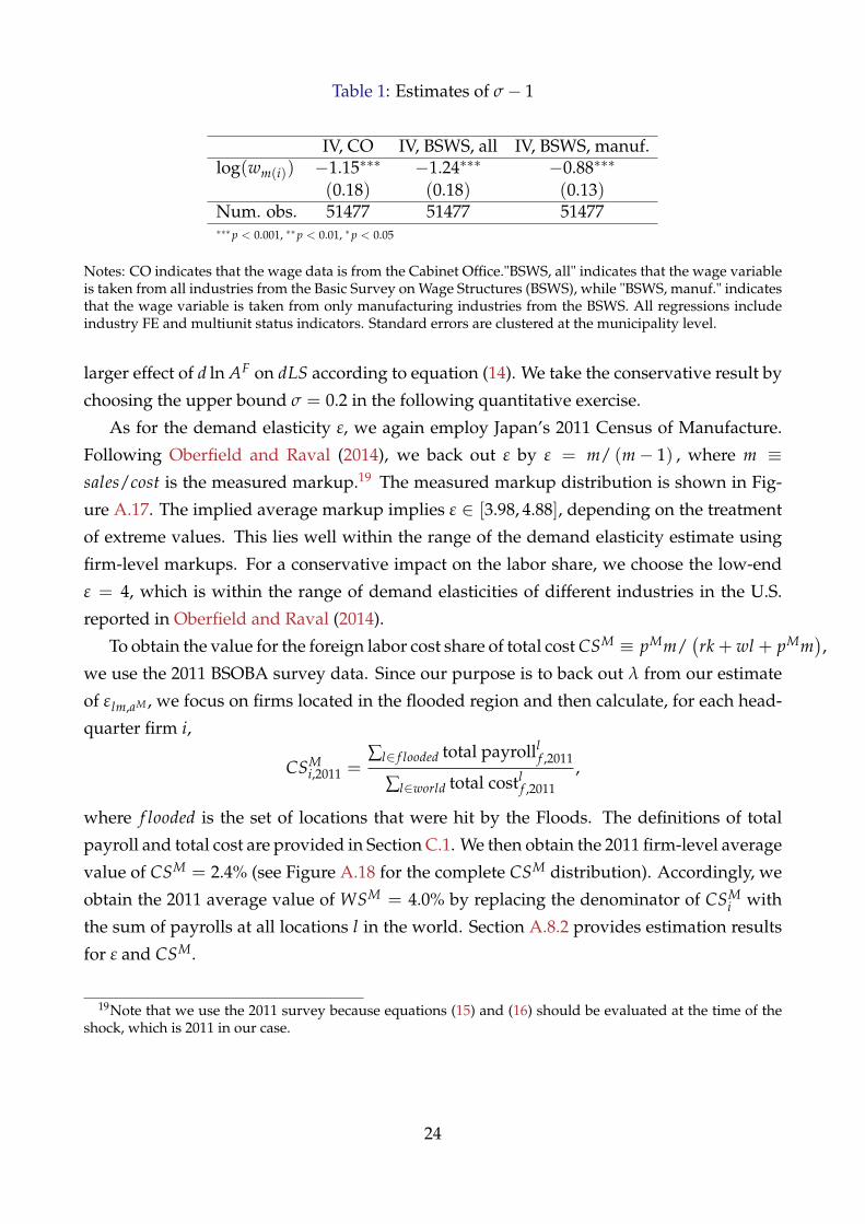
Table 1: Estimates of σ− 1

IV, CO IV, BSWS, all IV, BSWS, manuf.log(wm(i)) −1.15∗∗∗ −1.24∗∗∗ −0.88∗∗∗

(0.18) (0.18) (0.13)Num. obs. 51477 51477 51477∗∗∗p < 0.001, ∗∗p < 0.01, ∗p < 0.05

Notes: CO indicates that the wage data is from the Cabinet Office."BSWS, all" indicates that the wage variableis taken from all industries from the Basic Survey on Wage Structures (BSWS), while "BSWS, manuf." indicatesthat the wage variable is taken from only manufacturing industries from the BSWS. All regressions includeindustry FE and multiunit status indicators. Standard errors are clustered at the municipality level.

larger effect of d ln AF on dLS according to equation (14). We take the conservative result by

choosing the upper bound σ = 0.2 in the following quantitative exercise.

As for the demand elasticity ε, we again employ Japan’s 2011 Census of Manufacture.

Following Oberfield and Raval (2014), we back out ε by ε = m/ (m− 1) , where m ≡sales/cost is the measured markup.19 The measured markup distribution is shown in Fig-

ure A.17. The implied average markup implies ε ∈ [3.98, 4.88], depending on the treatment

of extreme values. This lies well within the range of the demand elasticity estimate using

firm-level markups. For a conservative impact on the labor share, we choose the low-end

ε = 4, which is within the range of demand elasticities of different industries in the U.S.

reported in Oberfield and Raval (2014).

To obtain the value for the foreign labor cost share of total cost CSM ≡ pMm/(rk + wl + pMm

),

we use the 2011 BSOBA survey data. Since our purpose is to back out λ from our estimate

of ε lm,aM , we focus on firms located in the flooded region and then calculate, for each head-

quarter firm i,

CSMi,2011 =

∑l∈ f looded total payrolllf ,2011

∑l∈world total costlf ,2011

,

where f looded is the set of locations that were hit by the Floods. The definitions of total

payroll and total cost are provided in Section C.1. We then obtain the 2011 firm-level average

value of CSM = 2.4% (see Figure A.18 for the complete CSM distribution). Accordingly, we

obtain the 2011 average value of WSM = 4.0% by replacing the denominator of CSMi with

the sum of payrolls at all locations l in the world. Section A.8.2 provides estimation results

for ε and CSM.

19Note that we use the 2011 survey because equations (15) and (16) should be evaluated at the time of theshock, which is 2011 in our case.

24

4.2.2 Step 2: Estimating λ by Natural Experiment

For obtaining λ by Equation (18), our goal is to estimate the left-hand side parameter σlm,aM .

In our empirical application, we specify H = JPN and F = ROW. We measure foreign

factor employment mit by total foreign labor employment since in our data, the quantity

of factor employment is only available for labor. We thus specify the factor substitution

between country H and F in the model as the substitution of labor across countries. As

discussed further below, our result is robust to other choices for measuring mit. Hence, we

use the notation l JPN as employment in Japan and lROW as employment in the rest of the

world, measuring factor employment in the rest of the world.

We run the following regression

ln(

l JPNit

)= ai + at + b ln

(lROWit

)+ eit, (21)

where ln(

l JPNit

)is log of firm i in year t, ln

(lROWit

)is the log factor employment in the rest

of the world, ai and at are firm- and year-fixed effects, and eit is the error term.

It is critical to control these rich fixed effects. In fact, controlling firm fixed effects restricts

ourselves to leverage within-firm variations, since high-productivity firms are likely to hire

workers in the ROW (or conduct FDI and become an MNE, as in Helpman et al., 2004). On

the other hand, controlling for year fixed effects enhances the validity of our analysis given

the economic environment in which an increasing number of firms become MNEs and hire

more local workers in foreign countries, as we saw in Figure 3.

In the data, the variation in the explanatory variable ln(lROWit

)can emerge from many

sources, one of which is the firm-specific exchange rate that occurs through demand shocks

or total factor productivity. Since we look for a foreign factor-augmenting productivity

shock in equation (17), we construct an instrumental variable (IV) based on the 2011 Thai-

land Floods. For this purpose, note that the flooding was local, it occurred during one

limited period of time relative to the coverage of our dataset and, most importantly, it was

unexpected. We construct an IV that interacts in the Thailand location before the flood and

the year after the flood. Because the shock was unexpected, the IV is exogenous to firms’

foreign production decisions, after controlling for the firm and year fixed effects. To lever-

age the variation in ln(lROWit

)caused by this foreign productivity shock, an IV of a shock

intensity measure is used:

Zit ≡l f loodedi,2011

l JPNi,2011 + lROW

i,2011

× 1 {t ≥ 2012} , (22)

where l f loodedi,2011 is firm-i’s total employment in the flooded regions in year 2011, right before

25

the flooding. This measure captures how much each MNE i relies on employment in the

flooded region. Namely, if a firm hires a relatively large number of workers in the flooded

region immediately before the flood, the firm is likely to be hit by the flood severely, thus

receiving a large negative (firm-i) foreign factor-augmenting productivity shock.

Given this instrument, the two-stage least square (2SLS) estimator is based on the fol-

lowing equations:

ln(

lROWit

)= ai + at + bZit + eit, and (23)

ln(

l JPNit

)= ai + at + bZit + eit. (24)

Therefore, we expect the first stage regression will yield a negative correlation between

ln(lROWit

)and Zit conditional on the fixed effects. Given the validity of the first stage, we

interpret

bIV = σlm,aM .

As shown in Section 4.1.1, the floods had medium- to long-run effects rather than short-run

effects on employment, so coefficient bIV or, in turn, λ as meduim- to long-run elasticity

rather than short-run. Specifically, we relate the decline in employment found in aggregate

in Panel 3a as an exogenous-sourced decline in ROW log-employment ln(lROWit

), and relate

that to the change in log-employment in Home ln(

l JPNit

). This point is crucial when we

move on to the quantitative exercise, because our concern is a relatively long-run change in

labor share. In the discussion below, we conduct a robustness check of the long-difference

specification and extension to the event-study regressions.

Table 2 shows the estimation result from the 2SLS specification (23) and (24), with the

robust standard errors reported in parentheses. All columns show that the coefficients are

statistically significant at the two-sided one-percent level.

Column 1 shows the result of the OLS specification without any fixed effects; that is,

under the restriction ai = at = 0 for all i and t, column 2 the fixed effect specification, and

column 3 the instrumental variable specification in equation (22). Comparing Columns 1

and 2, we see that while both coefficients are positive, the coefficient magnitude becomes

small after controlling for fixed effects as to heterogeneity in the productivity of firms.

Column 3 shows that a one-percent decrease in employment in the rest of the world

due to the 2011 Thailand Floods caused Japanse MNEs to decrease home employment by

0.192 percent. Although this coefficient is a composite of model parameters as shown in

equation (18) without any meaningful interpretation by itself, it is produced by the 2SLS

first stage and reduced-form regressions shown in columns 4 and 5. Column 4 shows that

a firm that did not rely on employment in the flooded region in 2011 would have reduced

its employment in the rest of the world by 72.8 percent had it relied completely on the

26

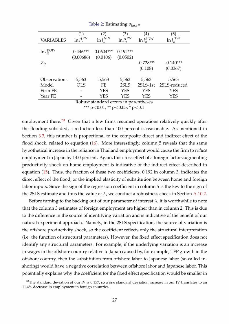
Table 2: Estimating σlm,aM

(1) (2) (3) (4) (5)VARIABLES ln l JPN

it ln l JPNit ln l JPN

it ln lROWit ln l JPN

it

ln lROWit 0.446*** 0.0604*** 0.192***

(0.00686) (0.0106) (0.0502)Zit -0.728*** -0.140***

(0.108) (0.0367)

Observations 5,563 5,563 5,563 5,563 5,563Model OLS FE 2SLS 2SLS-1st 2SLS-reducedFirm FE - YES YES YES YESYear FE - YES YES YES YES

Robust standard errors in parentheses*** p<0.01, ** p<0.05, * p<0.1

employment there.20 Given that a few firms resumed operations relatively quickly after

the flooding subsided, a reduction less than 100 percent is reasonable. As mentioned in

Section 3.3, this number is proportional to the composite direct and indirect effect of the

flood shock, related to equation (16). More interestingly, column 5 reveals that the same

hypothetical increase in the reliance in Thailand employment would cause the firm to reduce

employment in Japan by 14.0 percent. Again, this cross effect of a foreign factor-augmenting

productivity shock on home employment is indicative of the indirect effect described in

equation (15). Thus, the fraction of these two coefficients, 0.192 in column 3, indicates the

direct effect of the flood, or the implied elasticity of substitution between home and foreign

labor inputs. Since the sign of the regression coefficient in column 5 is the key to the sign of

the 2SLS estimate and thus the value of λ, we conduct a robustness check in Section A.10.2.

Before turning to the backing out of our parameter of interest λ, it is worthwhile to note

that the column 3 estimates of foreign employment are higher than in column 2. This is due

to the difference in the source of identifying variation and is indicative of the benefit of our

natural experiment approach. Namely, in the 2SLS specification, the source of variation is

the offshore productivity shock, so the coefficient reflects only the structural interpretation

(i.e. the function of structural parameters). However, the fixed effect specification does not

identify any structural parameters. For example, if the underlying variation is an increase

in wages in the offshore country relative to Japan caused by, for example, TFP growth in the

offshore country, then the substitution from offshore labor to Japanese labor (so-called in-

shoring) would have a negative correlation between offshore labor and Japanese labor. This

potentially explains why the coefficient for the fixed effect specification would be smaller in

20The standard deviation of our IV is 0.157, so a one standard deviation increase in our IV translates to an11.4% decrease in employment in foreign countries.

27

magnitude than that for 2SLS.

Based on the calibrations of σ and ε from Section 4.2.1, equation (17) implies that λ = 1.4.

Since ε lm,aM has a valid standard error from the 2SLS estimation, we can obtain the standard

error of λ as 0.13 by the Delta method, indicating that we reject the gross-complementary

home and foreign labor λ ≤ 1 at the 0.1 percent significance level, as discussed in detail

in Section A.9. Therefore, our calibrations σ = 0.2 and λ = 1.4 imply that Assumption

1 is satisfied empirically. Applying Lemma 1, we conclude that a positive foreign factor

augmentation causes a qualitative decrease in labor share. To proceed to the quantitative

implication, in what follows we back out the foreign factor augmentation from the aggregate

data.

In Section A.10 of the Appendix, we discuss a number of robustness checks, including

use of other measures of MNEs like foreign operation at extensive margins and subsidiary

sales, choice of control groups, and the role of Tohoku Earthquake and tsunami. In Section

A.11, we also show some extension exercises, such as the use of widely-used shift-share

instruments, event study-style regression analysis, substitution between Thailand and other

third countries, and industry-specific effects.

5 Discussions

5.1 Quantitative Implication of Foreign Factor Augmentations

In Section 4, we discussed how we backed out the elasticity of labor share with respect to

the foreign factor augmentation. To derive the implication quantitatively, we need to know

how much foreign factor-augmenting productivity grew over the period of interest. For

this purpose, we invert the factor demand functions (B.43) and (B.44) in the aggregate. We

proxy the quantity of employment of foreign factors M by the foreign employment LROW

and accordingly the foreign factor prices by labor wage wROW . We apply H = JPN and

F = ROW to obtain21

aM

aL =

(LROW

LJPN

) 1λ−1(

wROW

wJPN

) λλ−1

. (25)

Therefore, given the measures of aggregate employment and average wage in the home and

foreign countries, and the backed-out elasticity between home and foreign labor, we can

obtain the implied relative productivity in the rest of the world. The intuition behind the

relationship is as follows. Suppose, as we calibrated, λ > 1, or factor augmentation is biased

to that factor. Then given the wage structure in the rest of the world and Japan, relatively

21It is an important extension to consider a multi-country version of our model and its empirical implemen-tations. Section A.7.1 reviews the country-level aggregate trends.

28

large employment in the rest of the world implies relatively augmentingly productive labor

in the rest of the world. On the other hand, given the employment structure, a relatively

high wage in the rest of the world also reflects relatively augmentingly productive labor in

the rest of the world.22 We measure(

LROW , wROW) by BSOBA. In particular, we calculate

LROW by aggregating all foreign employment in all countries except for Japan and wROW by

dividing the aggregate total labor compensation by LROW . For(

LJPN, wJPN), we apply the

JIP database, a Japanese project for assembling KLEMS database.

To obtain the absolute productivity aM as opposed to the relative productivity aM/aL,

we calibrate Japan’s labor-augmenting productivity growth by JIP database’s Quality of La-

bor measure. The JIP measure reflects changes in the composition of workers–gender, age,

education, employment status– which is standard representation of factor augmentation.

We argue that this affects the efficiency units of labor, thereby Japan’s labor-augmenting

productivity. Given this trend, we can separate the trends of factor augmentation in Japan

and the rest of the world. As a result, in Figure 5a, the left panel shows the trend of the

evolution of d ln aMt ≈ ln aM

t − ln aM1995, with our base year 1995, while Figure C.1 shows the

growth in Japan’s labor augmentation.

We emphasize the relative importance of d ln aMt and d ln aL

t . By comparing the y-axes,

we confirm that the growth d ln aL is relatively minor in the relative factor augmentation

evolution d ln(aM/aL) = d ln aM− d ln aL in equation (25). This could be interpreted as due

to at least two factors. First, the relative augmentation was fast in the rest of the world rela-

tive to in Japan. This is plausible given that our BSOBA-based measure of LROW and wROW ,

the ingredients in equation (25), comes from employment data in many rapidly expanding

economies including Thailand. Second, globalization may contribute to the relative impor-

tance of d ln aM, comprising declining transportation and communication costs as well as

the removal of political barriers to investment. These imply higher employment in the rest

of the world by Japanese MNEs given the factor costs, according to our estimated elasticity

of substitution λ = 1.4.

With these calibrations, we may learn the evolution of the effect of foreign factor aug-

mentation on labor share. We calculate WSM0 as the fraction of total payment to foreign

labor taken from BSOBA over the sum of that and the total payment to workers in Japan in

the base year, which gives WSM0 = 0.8%. In Figure 5b, we show the counterfactual labor

share had there been only the foreign augmentation from equation (14). Again, we set the

base year to 1995, the first year of the BSOBA data. The solid line shows the actual evolu-

tion, whereas the dashed line shows the counterfactual one, and we see that foreign factor

22Note our qualification λ > 1. In fact, if λ < 1, then the discussion in the text reverses, which meansthat an observed increase in foreign employment and wages would imply decreasing relative foreign factoraugmentation. To the extent that such a decrease is implausible, this observation is more supporting evidencefor λ > 1. Section C.1.2 shows the implication to AROW when it is nonetheless assumed that λ < 1.

29

Figure 4: Quantitative Implications

(a) Foreign Factor Augmentation d ln AF (b) Actual and Counterfactual Labor Share

augmentation played a substantial role in explaining the observed labor share decline from

1995-2007. Quantitatively, it explains 59 percent of the decline during the period.

Discussion One might naturally ask whether this large effect is an artifact of our choice

of sample period. We chose a baseline final year of 2007 for our analysis both because

the Great Recession would complicate the interpretation and also because the international

System of National Accounts (SNA) changed drastically after 2008. However, Section C.2

shows the corresponding results for a more recent trend in labor share up to 2015,23 and

we find that 58 percent of the decrease in labor share from 1995 to 2015 may be attributed

to our mechanism of increased foreign productivity. Our mechanism is also successful in

explaining the countercyclical component of labor share trend in the data.

We also conduct the same quantitative analysis from peak to peak to further control

for potential effects of business cycle. We take peak years, 1997, 2000, and 2008, from the

Cabinet Office of Japan. When we conduct the quantitative analysis from 1997 to 2008 and

2000 to 2008, our mechanism could explain the decrease in the labor share by 77 percent and

112 percent. The reason we obtain large values for the recent waves of the business cycle is

that the actual decrease in the labor share was small, especially between 2000 and 2008, so

the fraction that our mechanism explains becomes large.

Finally, we investigate how our quantitative results may differ given the error in the

estimate of our key parameter, λ. To do this, we use the standard error estimate se(λ) =

0.13 that we derive in Section A.9 of the Appendix. In particular, we conduct the same

quantitative analysis with values of λ one standard error smaller and larger. The results

indicate that the quantitative magnitude relative to the observed decrease in the labor share

23As a reservation, the quantitative result is sensitive to our parameter values, in particular the estimate ofσ. Section C.1.3 shows different results under several parameter values of λ and σ.

30

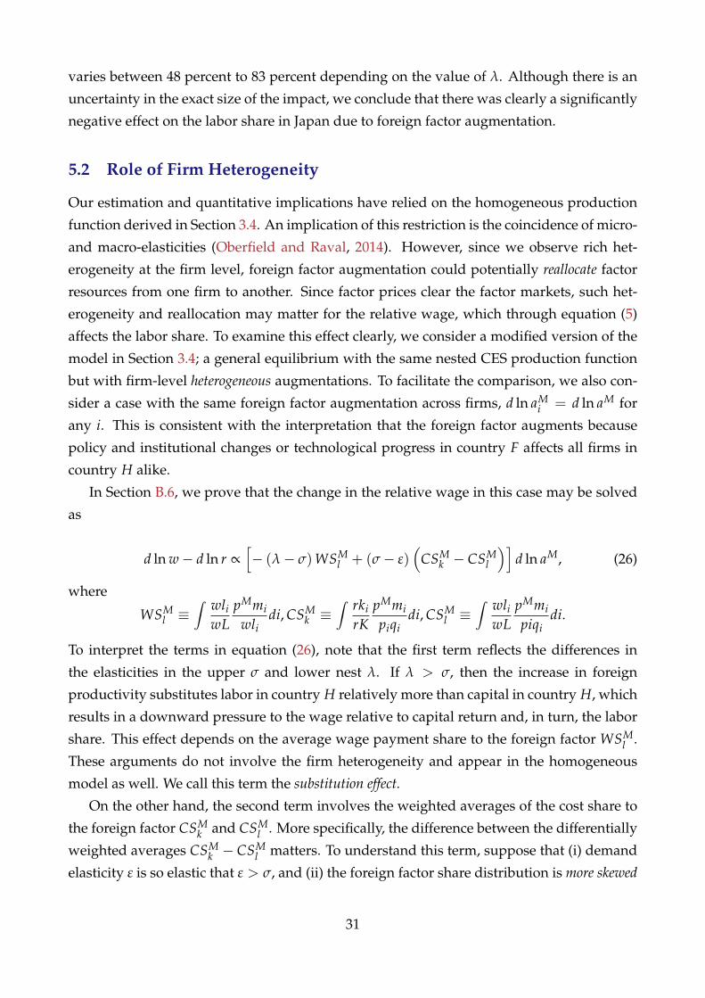
varies between 48 percent to 83 percent depending on the value of λ. Although there is an

uncertainty in the exact size of the impact, we conclude that there was clearly a significantly

negative effect on the labor share in Japan due to foreign factor augmentation.

5.2 Role of Firm Heterogeneity

Our estimation and quantitative implications have relied on the homogeneous production

function derived in Section 3.4. An implication of this restriction is the coincidence of micro-

and macro-elasticities (Oberfield and Raval, 2014). However, since we observe rich het-

erogeneity at the firm level, foreign factor augmentation could potentially reallocate factor

resources from one firm to another. Since factor prices clear the factor markets, such het-

erogeneity and reallocation may matter for the relative wage, which through equation (5)

affects the labor share. To examine this effect clearly, we consider a modified version of the

model in Section 3.4; a general equilibrium with the same nested CES production function

but with firm-level heterogeneous augmentations. To facilitate the comparison, we also con-

sider a case with the same foreign factor augmentation across firms, d ln aMi = d ln aM for

any i. This is consistent with the interpretation that the foreign factor augments because

policy and institutional changes or technological progress in country F affects all firms in

country H alike.

In Section B.6, we prove that the change in the relative wage in this case may be solved

as

d ln w− d ln r ∝[− (λ− σ)WSM

l + (σ− ε)(

CSMk − CSM

l

)]d ln aM, (26)

where

WSMl ≡

∫ wliwL

pMmi

wlidi, CSM

k ≡∫ rki

rKpMmi

piqidi, CSM

l ≡∫ wli

wLpMmi

piqidi.

To interpret the terms in equation (26), note that the first term reflects the differences in

the elasticities in the upper σ and lower nest λ. If λ > σ, then the increase in foreign

productivity substitutes labor in country H relatively more than capital in country H, which

results in a downward pressure to the wage relative to capital return and, in turn, the labor

share. This effect depends on the average wage payment share to the foreign factor WSMl .

These arguments do not involve the firm heterogeneity and appear in the homogeneous

model as well. We call this term the substitution effect.

On the other hand, the second term involves the weighted averages of the cost share to

the foreign factor CSMk and CSM

l . More specifically, the difference between the differentially

weighted averages CSMk − CSM

l matters. To understand this term, suppose that (i) demand

elasticity ε is so elastic that ε > σ, and (ii) the foreign factor share distribution is more skewed

31

to capital intensive firms than it is to Home labor intensive firms, or CSMk − CSM

l > 0.

Note that assumption (ii) is consistent with the finding by Sun (2020) that “multinational

firms are on average larger firms and larger firms on average use more capital-intensive

technologies.” Given these two assumptions, the increase in the foreign factor productivity

results in a reduction in the marginal cost of production, which causes high demand if ε

is large. Across firms, this is moreso for firms that use relatively more foreign factors. If

such firms are more capital intensive than Home labor intensive, the aggregate demand for

capital increases more than that for Home labor. This causes the capital return to increase

more than the Home wage, which results in a reduction in the labor share. We call this effect

the reallocation effect. Note that the argument above crucially depends on the heterogeneity

in firms’ factor intensities. Indeed, if firms are homogeneous, the weight of the weighted

average of cost shares does not matter, so that CSMk − CSM

l = CSM − CSM = 0. Therefore,

when there is no heterogeneity in firm factor intensity, there is no reallocation effect and the

effect on the Home relative wage only emerges as the substitution effect.

To measure the size of the substitution and reallocation effects, we employ our matched

dataset. BSJBSA data contains the variable of cost of labor compensation in the domestic

firms and net operating surplus. We take these measures as wli and rki, respectively. From

BSOBA, we can obtain the total compensation of MNEs in each foreign plant, which we

aggregate to form a measure of pMmi. We match these datasets and calculate CSMk , CSM

l ,

and WSMl that are relevant in equation (26). The matched data is available for 2007-2016.

With values λ = 1.4, σ = 0.2, ε = 4, we plot the size of the substitution and reallocation

effects according to data from each year (Figure 5).

Figure 5 provides two takeaways. First, both the substitution and reallocation effects are

negative for most years. Indeed, except for the reallocation effect in 2015, all effects head to

the negative side. This implies that when foreign factor productivity increases, the relative

Home wage decreases, which pushes down the Home labor share. Moreover, introducing

heterogeneity into the model strengthens the negative effect of a given increase in the for-

eign productivity due to the reallocation effect. Note that the substitution effect is negative

because λ > σ. The reallocation effect is mostly negative both because (i) ε > σ and (ii) in

most of the years CSMk > CSM

l in the data. Second, in many years, the reallocation effect

is smaller than the substitution effect in absolute value. Therefore, although the realloca-

tion amplifies the negative substitution effect, it does not contribute to the overall effect in

a dominant way.24 Combining these two observations, we conclude that firm heterogeneity

and the reallocation effect does not alter our conclusion that foreign factor augmentation

worked as a force that decreased the labor share in Japan from 1995-2007.

24One may see relatively high volatility of the reallocation effect. This is due in part to the fact that wemeasure the capital payment by accounting net operating surplus which is volatile.

32

Figure 5: Relative Size of the Effects

Note: The 2007-2016 trend of the relative size of the reallocation effect and substitution effects among the dropin the labor share. The reallocation effect is the component due to firms’ heterogeneous factor inputs, and thesubstitution effect shows the capital-labor substitution given the relative factor price changes within a firm.See the main text for the detail.

5.3 Method of Moments Estimation

In this section, we apply the estimation method based on the general moment conditions

(9). For this purpose, we take a two-step approach. First, we separate the set of parame-

ters estimated by equation (9) and other nuisance parameters.25 We then fix the nuisance

parameters by the method based on the nested CES specification discussed so far. Second,

given these parameters, we identify and estimate the parameters of our interest.

In particular, given the elasticity matrix discussed in Section B.5, for all i, we set σkr,i =

−σ + (σ− ε)CSKi , σkw,i = (σ− ε)CSL

i , σlr,i = (σ− ε)CSKi , σlw,i = −λ + (λ− σ)WSL

i +

(σ− ε)CSLi , σ

mpM,i= −λ + (λ− σ)WSM

i + (σ− ε)CSMi , where σ and λ are constants re-

flecting the substitution parameters under nested CES, CS fi are firm i’s factor- f cost share for

f = K, L, M, and WS fi are firm i’s factor- f payment share between L and M for f = L, M. We

take CS fi and WS f

i from our firm-level Japanese MNE data, and calibrate λ = 1.4, σ = 0.2,

and ε = 4.

We then estimate the remaining parameters, elasticities of country-H capital and labor

demand with respect to foreign factor prices. We employ the method of moments (9) and the

flood-based instrumental variable. In particular, first, to have restrictions on σmr,i and σmw,i,

note that by the symmetry of the Hessian matrix of the cost function, demand structure (1),

and Shephard’s lemma, we have

CSMi σmr,i = CSK

i σkpM,i

, (27)

25Section C.3 discusses the estimation of standard errors of the estimator defined by equation (9).

33

CSMi σml,i = CSL

i σl pM,i

. (28)

Proof of these equations is given in Section B.7. Finally, to implement the estimation, we

assume the following constant parameter assumption.

Assumption 2. σkpM,i

= σkpM and σ

l pM,i= σ

l pM for all i ∈ IH.

Given this setup, we implement the method of moments estimation based on equation

(9) as follows.

1. Set n = 0. Guess(

σkpM , σ

l pM

)=

(σ(n)

k pM, σ

(n)

l pM

)and generate implied firm-level elastic-

ity matrix Σ(n) based on equation (10) and our set of partial identification assumptions

and the factor augmentation d ln

(aK,(n)

it

)d ln

(aL,(n)

it

)d ln

(aM,(n)

it

)

based on equation (11).

2. Remove the year fixed effects from the factor augmentation and instrumental variables

Zit.

3. Evaluate the sample-analog of the moment condition (9).

4. If a closed-form solution is not obtained, update n, go back to process 1 and iterate

until convergence.

Out of the above algorithm, we obtain

σkpM = −0.20 (std. err. 0.13), (29)

σl pM = −0.09 (std. err. 0.04). (30)

Recall that our finding that the capital demand is more elastic, σkpM < σ

l pM , suggests that

a negative cost shock (or positive factor augmentation) increases the demand for Home

capital relatively more than Home labor. Given that capital demand is more negatively elastic

to the capital rental rate and labor demand is to wage, the capital rental rate must increase

while the wage for labor must decrease to restore the factor market clearing conditions (3).

Note that the last part of this logic is reminiscent of the celebrated Stolper-Samuelson

theorem: Consider a two-factor economy. If the factor demand increases differentially for one

factor, then the relative wage of that factor increases (more than the increase in the factor

demands) while the wage of the other decreases. In the Stolper-Samuelson setup, the factor

34

demand increase is caused by an exogenous change in the terms of trade. On the other hand,

in our setup, what drives the changes in factor demands in H is the combination of foreign

factor augmentation and (total) elasticity with respect to it of factors in H. If (same-sized)

foreign factor augmentation elastically increases the relative demand for one factor (in our

empirical case, capital relative to labor), that means that the demand for the factor increases

differentially, or the factor is complementary to the foreign factor that was augmented.

6 Conclusion

What impact does increased employment of foreign factors of production by an MNE have

on labor share in the home country? To address this question, we proceeded in three steps.

First, we developed an equilibrium model of production featuring augmented employment

of foreign factors with varying elasticities of substitution. From this theory, we then pin-

pointed the key elasticities relevant to labor share: the relative size of labor, and capital

substitution with foreign factors, and showed how a foreign factor-augmenting produc-

tivity shock to a small set of firms may help to identify these elasticities. Armed with these

theoretical results, we then applied the theory to the 2011 Thailand Floods, which was expe-

rienced as a large negative foreign factor productivity shock for a subset of Japanese MNEs.

Using firm- and plant-level data from Japan, we estimated the reduced-form parameter

with the instrumental variable related to the flood shock, finding that home and foreign

labor are gross substitutes. This estimate, combined with the estimates of capital-labor elas-

ticity based on our Japanese plant-level data, indicates that foreign factor augmentation

contributed to the decline in the labor share in Japan from 1995-2007. Our further quantita-

tive counterfactual analyses show that 59 percent of the observed labor share decline in the

period can be attributed to foreign factor augmentation.

There are at least three different directions for extending the model. First, we may incor-

porate rich heterogeneity at the firm level as discussed in Section B.6 and at the destination

country level as we empirically suggest in Section A.7.1. Second, our production model

could potentially generalize an influential model of factor offshoring such as Feenstra and

Hanson (1997), which would tighten the connection with the literature. For this purpose, we

suggest a generalized production function in Section B.2. Finally, while our model extends

to a more complete general equilibrium with factor supplies and a large open economy, all

of the results of this paper in terms of identification, empirical application, and quantifica-

tion depend on the specific model choice, so this is another theoretical development left for

future study.

35

References

Acemoglu, Daron, “Why do new technologies complement skills? Directed technical

change and wage inequality,” The Quarterly Journal of Economics, 1998, 113 (4), 1055–1089.

and Pascual Restrepo, “Automation and New Tasks: How Technology Displaces and

Reinstates Labor,” Technical Report, National Bureau of Economic Research 2019.

Adachi, Daisuke, Daiji Kawaguchi, and Yukiko U. Saito, “Robot, Employment, and Pop-

ulation: Evidence from Articulated Robot in Japan’s Local Labor Markets,” Technical Re-

port, ESRI Working Paper 2019.

, Hiroyuki Nakata, Yasuyuki Sawada, and Kunio Sekiguchi, “Adverse Selection and

Moral Hazard in the Corporate Insurance Market: Evidence from the 2011 Thailand

floods,” Technical Report, Research Institute of Economy, Trade and Industry (RIETI)

2016.

Adao, Rodrigo, Costas Arkolakis, and Federico Esposito, “Spatial Linkages, Global

Shocks, and Local Labor Markets: Theory and Evidence,” 2018.

Arkolakis, Costas, Natalia Ramondo, Andres Rodrıguez-Clare, and Stephen Yeaple, “In-

novation and Production in the Global Economy,” 2017.

Autor, David, David Dorn, Lawrence F Katz, Christina Patterson, and John Van Reenen,

“Concentrating on the Fall of the Labor Share,” American Economic Review, 2017, 107 (5),

180–85.

, , , , and , “The fall of the labor share and the rise of superstar firms,” 2017.

Barkai, Simcha, “Declining labor and capital shares,” University of Chicago, 2017.

Benguria, Felipe and Alan M Taylor, “After the Panic: Are Financial Crises Demand or

Supply Shocks? Evidence from International Trade,” Working Paper 25790, National Bu-

reau of Economic Research April 2019.

Berger, David W, Kyle F Herkenhoff, and Simon Mongey, “Labor Market Power,” Techni-

cal Report, National Bureau of Economic Research 2019.

Bernard, Andrew B, Teresa C Fort, Valerie Smeets, and Frederic Warzynski, “Heteroge-

neous Globalization: Offshoring and Reorganization,” 2018.

Boehm, Christoph E, Aaron Flaaen, and Nitya Pandalai-Nayar, “Input Linkages and the

Transmission of Shocks: Firm-Level Evidence from the 2011 Tohoku Earthquake,” Review

of Economics and Statistics, 2018, (00).

36

, , and , “Multinationals, offshoring, and the decline of US manufacturing,” Journal of

International Economics, 2020, 127, 103391.

Brainard, S Lael and David A Riker, “Are US multinationals exporting US jobs?,” Technical

Report, National bureau of economic research 1997.

Bridgman, Benjamin, “Is Labor’s Loss Capital’s Gain? Gross Versus Net Labor Shares,”

Macroeconomic Dynamics, 2018, 22 (08), 2070–2087.

Cette, G, L Koehl, and T Philippon, “Labor shares in Some Advanced Economies,” Tech-

nical Report, Working Paper 2019.

Desai, Mihir A, C Fritz Foley, and James R Hines, “Domestic effects of the foreign activities

of US multinationals,” American Economic Journal: Economic Policy, 2009, 1 (1), 181–203.

Ebenstein, Avraham, Ann Harrison, Margaret McMillan, and Shannon Phillips, “Esti-

mating the Impact of Trade and Offshoring on American Workers Using the Current Pop-

ulation Surveys,” The Review of Economics and Statistics, 2014, 96 (4), 581–595.

Elsby, Michael WL, Bart Hobijn, and Aysegul Sahin, “The decline of the US labor share,”

Brookings Papers on Economic Activity, 2013, 2013 (2), 1–63.

Feenstra, Robert C and Gordon H Hanson, “Foreign direct investment and relative wages:

Evidence from Mexico’s maquiladoras,” Journal of international economics, 1997, 42 (3), 371–

393.

Fort, Teresa C, Justin R Pierce, and Peter K Schott, “New perspectives on the decline of us

manufacturing employment,” Journal of Economic Perspectives, 2018, 32 (2), 47–72.

Gouin-Bonenfant, Emilien et al., “Productivity dispersion, between-firm competition and

the labor share,” 2018.

Gravelle, Jane G, “Tax Havens: International Tax Avoidance and Evasion,” 2015.

Handley, Kyle and Nuno Limao, “Policy uncertainty, trade, and welfare: Theory and evi-

dence for china and the united states,” American Economic Review, 2017, 107 (9), 2731–83.

Haraguchi, Masahiko and Upmanu Lall, “Flood risks and impacts: A case study of Thai-

land’s floods in 2011 and research questions for supply chain decision making,” Interna-

tional Journal of Disaster Risk Reduction, 2015, 14, 256–272.

Harrison, Ann and Margaret McMillan, “Offshoring jobs? Multinationals and US manu-

facturing employment,” Review of Economics and Statistics, 2011, 93 (3), 857–875.

37

Head, Keith and John Ries, “Offshore production and skill upgrading by Japanese manu-

facturing firms,” Journal of international economics, 2002, 58 (1), 81–105.

Helpman, Elhanan, Marc J Melitz, and Stephen R Yeaple, “Export versus FDI with hetero-

geneous firms,” American economic review, 2004, 94 (1), 300–316.

Hummels, David, Rasmus Jørgensen, Jakob Munch, and Chong Xiang, “The wage effects

of offshoring: Evidence from Danish matched worker-firm data,” American Economic Re-

view, 2014, 104 (6), 1597–1629.

Johnson, Robert C. and Guillermo Noguera, “Accounting for intermediates: Production

sharing and trade in value added,” Journal of International Economics, 2012, 86 (2), 224 –

236.

and , “A Portrait of Trade in Value-Added over Four Decades,” The Review of Economics

and Statistics, 2017, 99 (5), 896–911.

Kaldor, Nicholas, “Capital accumulation and economic growth,” in “The theory of capital,”

Springer, 1961, pp. 177–222.

Karabarbounis, Loukas and Brent Neiman, “The global decline of the labor share,” The

Quarterly journal of economics, 2013, 129 (1), 61–103.

Kato, Hayato and Toshihiro Okubo, “The Impact of a Natural Disaster on Foreign Direct

Investment and Vertical Linkages,” 2017.

Koh, Dongya, Raul Santaeulalia-Llopis, and Yu Zheng, “Labor Share Decline and Intellec-

tual Property Products Capital,” 2018.

Kovak, Brian K, Lindsay Oldenski, and Nicholas Sly, “The labor market effects of off-

shoring by us multinational firms: Evidence from changes in global tax policies,” Techni-

cal Report, National Bureau of Economic Research 2017.

Loecker, Jan De and Jan Eeckhout, “The rise of market power and the macroeconomic

implications,” Technical Report, National Bureau of Economic Research 2017.

Muendler, Marc-Andreas and Sascha O Becker, “Margins of multinational labor substitu-

tion,” The American Economic Review, 2010, 100 (5), 1999–2030.

Oberfield, Ezra and Devesh Raval, “Micro data and macro technology,” Technical Report,

National Bureau of Economic Research 2014.

Ottaviano, Gianmarco IP and Giovanni Peri, “Rethinking the effect of immigration on

wages,” Journal of the European economic association, 2012, 10 (1), 152–197.

38

Pierce, Justin R and Peter K Schott, “The surprisingly swift decline of US manufacturing

employment,” American Economic Review, 2016, 106 (7), 1632–62.

Piketty, Thomas and Gabriel Zucman, “Capital is back: Wealth-income ratios in rich coun-

tries 1700–2010,” The Quarterly Journal of Economics, 2014, 129 (3), 1255–1310.

Ramondo, Natalia and Andres Rodrıguez-Clare, “Trade, multinational production, and

the gains from openness,” Journal of Political Economy, 2013, 121 (2), 273–322.

, , and Felix Tintelnot, “Multinational production: Data and stylized facts,” American

Economic Review, 2015, 105 (5), 530–36.

Raval, Devesh R, “The micro elasticity of substitution and non-neutral technology,” The

RAND Journal of Economics, 2019, 50 (1), 147–167.

Rognlie, Matthew, “Deciphering the fall and rise in the net capital share: accumulation or

scarcity?,” Brookings papers on economic activity, 2016, 2015 (1), 1–69.

, “Comment on” Accounting for Factorless Income”,” in “NBER Macroeconomics Annual

2018, volume 33,” University of Chicago Press, 2018.

Setzler, Bradley and Felix Tintelnot, “The Effects of Foreign Multinationals on Workers

and Firms in the United States,” Technical Report, National Bureau of Economic Research

2019.

Slaughter, Matthew J, “Production transfer within multinational enterprises and American

wages,” Journal of international Economics, 2000, 50 (2), 449–472.

Steinberg, Joseph et al., “Brexit and the macroeconomic impact of trade policy uncertainty,”

in “2017 Meeting Papers” number 216 Society for Economic Dynamics 2017.

Sun, Chang, “Multinational production with non-neutral technologies,” Journal of Interna-

tional Economics, 2020, 123, 103294.

Tamada, Yoshifumi, Keisuke Hoshikawa, and Tsuruyo Funatsu, The 2011 Thailand Flood–

the record and lessons– (in Japanese), Japan External Trade Organization (JETRO) Asian In-

stitute, 2013.

Tolbert, Charles M and Molly Sizer, “US commuting zones and labor market areas: A 1990

update,” Technical Report 1996.

39

Online Appendix

A Data and Empirical Result Appendix

A.1 Further Data on Labor Share and Multinational Activities

Figure A.1 shows the longer-run trend of labor share in Japan since 1980 to complement

Figure 2 in the main text. Although there is a countercyclical component and a sag around

1990, the overall long-run trend reveals the same message as Figure 2: the persistent decline

in the labor share for the three decades.

While Figure A.1 is concerned about labor compensation, Figure A.3a shows the trends

of both labor and capital earnings by Japanese MNEs from the BSOBA data. Note that

capital income has been increasing since 1995, but the trend is more volatile than payment

to labor. This increase can partly explain the more rapid increase in GNI than GDP in Japan

because the income from the foreign capital is accounted for under the positive net primary

income from abroad. It will be a crucial step to explicitly allow foreign capital in our model.

A.2 Robust Labor Share Decrease

As explained in Section 1.1, neither the conceptual or operational measurement of labor

share is trivial. In this section, we provide several measures of the labor share in Japan be-

tween 1995 and 2007 to see that irrespective of the measurement process, we have robust

evidence that the labor share has been decreasing. First, the green line in Figure A.3b shows

our preferred measure, the total labor cost divided by GDP. However, since GDP or value

added includes capital depreciation, it overstates net capital income (Bridgman, 2018). To

overcome this, we take the SNA data from the Japan Cabinet Office Long-run Economic

Statistics and calculate the trend in the share of nominal employee compensation over nom-

inal national income, which excludes capital depreciation (as well as indirect tax, while

including subsidies). This trend is shown by the blue line. Another issue is the treatment

of the mixed income of self-employees. Since self-employees are typically owners of both

the production capital and labor, the allocation of the generated income to labor and capital

can be distorted (e.g., Rognlie, 2018). To remove any biases due to the misallocation of such

mixed income, we take the trend of domestic corporate factor income and their compensa-

tion payment to the labor, which is shown by the red line. We can see in Figure A.3b that all

of these trends are decreasing.

40

Figure A.1: Labor Share and Payment to Foreign Employment, Japan

Note: The authors’ calculation based on Japan Industrial Productivity (JIP) Database 2015 from Research Insti-tute of Economy, Trade and Industry (RIETI) and the Basic Survey on Overseas Business Activities (BSOBA)1996-2008. The labor share is calculated by the share of the nominal labor cost in the value added of JIP marketeconomies in nominal terms. The payment to foreign labor is the sum of compensation to workers in foreignsubsidiaries of all Japanese multinational corporations in BSOBA.

A.3 Comparison of MNEs and Non-MNEs

To further analyze the role of MNEs in the decrease in labor share, we conduct a simple

decomposition analysis across MNEs and non-MNEs by aggregating total sales, labor com-

pensation and net income separately for MNEs and non-MNEs. We then calculate the labor

share for the two groups. Figure A.3 shows the trends for labor share and MNE composi-

tion. The blue line depicts the trends in the share of the sum of MNE HQ sales relative to the

sum of sales of all firms. In 1995, the share was roughly 12 percent, which rose to close to 15

percent in 2007. Therefore, the composition of sales became skewed toward MNEs over the

period. The red lines show the labor share trends among MNEs (solid line) and non-MNEs

(dashed line), and we can see that the labor share of MNEs decreases more rapidly. Addi-

tionally, throughout the period, MNEs had a lower labor share than non-MNEs. Since the

labor share composition by MNEs increased (as shown by the blue line), both of these facts

have contributed to the decrease in aggregate labor share.

One of the interpretations of these facts is that within MNEs, the payment to labor rel-

ative to capital decreased over the period, and more firms become MNEs. In the model

section, we develop a framework in which both of these may be explained by foreign factor

augmentation.

41

Figure A.2: MNE Activities and Labor Shares, Detailed

(a) Earnings by Foreign Labor and Capital (b) Labor Share Measures in Japan, 1995-2007

Note: The authors’ calculation based on the Basic Survey on Overseas Business Activities (BSOBA) 1996-2017,the 2015 Japan Industrial Productivity (JIP) Database, Cabinet Office Long-Run Economic Statistics (COLES,https://www5.cao.go.jp/j-j/wp/wp-je12/h10 data01.html, accessed on May 13, 2019), and Japan SNA, Gen-eration of Income Account, 2009. The left panel shows the trends of the total profit and labor compensationin the foreign subsidiaries of all Japanese MNEs. Foreign subsidiary profit is the sum of current net profit ofall subsidiaries of Japanese multinational corporations in BSOBA, and payment to offshore labor is the sum ofworker compensation to foreign subsidiaries of all Japanese multinational corporations in BSOBA. The rightpanel shows labor share trends in Japan from several sources. JIP-based labor share is calculated by the shareof nominal labor cost in the nominal value added of JIP market economies. National income-based laborshare is the fraction of nominal employee compensation over nominal national income from COLES. Domes-tic corporate-based labor share is the net labor share of domestic corporate factor income, calculated from theSNA by the fraction of the item “Wages and salaries” over the sum of “Wages and salaries” and “Operatingsurplus, net.”

A.4 Other Potential Mechanisms

There are several mechanisms behind decreasing labor shares proposed in the literature.

I review some first-pass evidence that neither of recent automation and surge in market

powers is likely to play a main role in explaining shrinking labor share.

Automation in Japan As discussed in Section 1.1, bias in technological change can arise

from at least two sources: automation and offshoring. Since the current paper focuses on

offshoring; in particular, factor offshoring as opposed to goods offshoring (Hummels et al.,

2014), the evolution of automation technology in Japan is not our main focus. However, by

examining the aggregate data used in automation literature (e.g., Acemoglu and Restrepo,

2019), we see suggestive evidence that automation acceleration was not observed in Japan

as rapidly as in other highly automating countries from the 1990s to 2010s.

To examine this, we employ data from the International Federation of Robotics (IFR) to ob-

tain the operational stock of industrial robots in each country by year. Figure A.5a shows the

trends for the five most robot-adopting countries (China, Japan, United States, South Korea,

Germany). All countries other than Japan rapidly introduced industrial robots from 1993

42

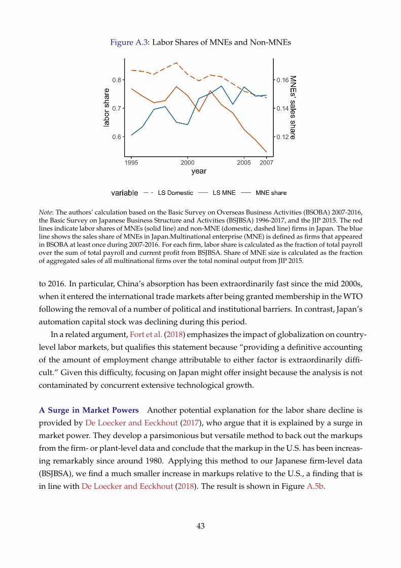
Figure A.3: Labor Shares of MNEs and Non-MNEs

Note: The authors’ calculation based on the Basic Survey on Overseas Business Activities (BSOBA) 2007-2016,the Basic Survey on Japanese Business Structure and Activities (BSJBSA) 1996-2017, and the JIP 2015. The redlines indicate labor shares of MNEs (solid line) and non-MNE (domestic, dashed line) firms in Japan. The blueline shows the sales share of MNEs in Japan.Multinational enterprise (MNE) is defined as firms that appearedin BSOBA at least once during 2007-2016. For each firm, labor share is calculated as the fraction of total payrollover the sum of total payroll and current profit from BSJBSA. Share of MNE size is calculated as the fractionof aggregated sales of all multinational firms over the total nominal output from JIP 2015.

to 2016. In particular, China’s absorption has been extraordinarily fast since the mid 2000s,

when it entered the international trade markets after being granted membership in the WTO

following the removal of a number of political and institutional barriers. In contrast, Japan’s

automation capital stock was declining during this period.

In a related argument, Fort et al. (2018) emphasizes the impact of globalization on country-

level labor markets, but qualifies this statement because “providing a definitive accounting

of the amount of employment change attributable to either factor is extraordinarily diffi-

cult.” Given this difficulty, focusing on Japan might offer insight because the analysis is not

contaminated by concurrent extensive technological growth.

A Surge in Market Powers Another potential explanation for the labor share decline is

provided by De Loecker and Eeckhout (2017), who argue that it is explained by a surge in

market power. They develop a parsimonious but versatile method to back out the markups

from the firm- or plant-level data and conclude that the markup in the U.S. has been increas-

ing remarkably since around 1980. Applying this method to our Japanese firm-level data

(BSJBSA), we find a much smaller increase in markups relative to the U.S., a finding that is

in line with De Loecker and Eeckhout (2018). The result is shown in Figure A.5b.

43

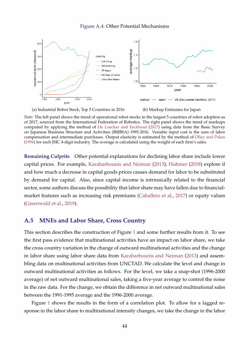
Figure A.4: Other Potential Mechanisms

(a) Industrial Robot Stock, Top 5 Countries in 2016 (b) Markup Estimates for Japan

Note: The left panel shows the trend of operational robot stocks in the largest 5 countries of robot adoption asof 2017, sourced from the International Federation of Robotics. The right panel shows the trend of markupscomputed by applying the method of De Loecker and Eeckhout (2017) using data from the Basic Surveyon Japanese Business Structure and Activities (BSJBSA) 1995-2016. Variable input cost is the sum of laborcompensation and intermediate purchases. Output elasticity is estimated by the method of Olley and Pakes(1996) for each JSIC 4-digit industry. The average is calculated using the weight of each firm’s sales.

Remaining Culprits Other potential explanations for declining labor share include lower

capital prices. For example, Karabarbounis and Neiman (2013); Hubmer (2018) explore if

and how much a decrease in capital goods prices causes demand for labor to be substituted

by demand for capital. Also, since capital income is intrinsically related to the financial

sector, some authors discuss the possibility that labor share may have fallen due to financial-

market features such as increasing risk premiums (Caballero et al., 2017) or equity values

(Greenwald et al., 2019).

A.5 MNEs and Labor Share, Cross Country

This section describes the construction of Figure 1 and some further results from it. To see

the first pass evidence that multinational activities have an impact on labor share, we take

the cross country variation in the change of outward multinational activities and the change

in labor share using labor share data from Karabarbounis and Neiman (2013) and assem-

bling data on multinational activities from UNCTAD. We calculate the level and change in

outward multinational activities as follows. For the level, we take a snap-shot (1996-2000

average) of net outward multinational sales, taking a five-year average to control the noise

in the raw data. For the change, we obtain the difference in net outward multinational sales

between the 1991-1995 average and the 1996-2000 average.

Figure 1 shows the results in the form of a correlation plot. To allow for a lagged re-

sponse in the labor share to multinational intensity changes, we take the change in the labor

44

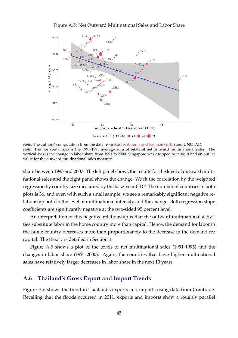
Figure A.5: Net Outward Multinational Sales and Labor Share

Note: The authors’ computation from the data from Karabarbounis and Neiman (2013) and UNCTAD.Note: The horizontal axis is the 1991-1995 average sum of bilateral net outward multinational sales. Thevertical axis is the change in labor share from 1991 to 2000. Singapore was dropped because it had an outliervalue for the outward multinational sales measure.

share between 1995 and 2007. The left panel shows the results for the level of outward multi-

national sales and the right panel shows the change. We fit the correlation by the weighted

regression by country size measured by the base-year GDP. The number of countries in both

plots is 36, and even with such a small sample, we see a remarkably significant negative re-

lationship both in the level of multinational intensity and the change. Both regression slope

coefficients are significantly negative at the two-sided 95 percent level.

An interpretation of this negative relationship is that the outward multinational activi-

ties substitute labor in the home country more than capital. Hence, the demand for labor in

the home country decreases more than proportionately to the decrease in the demand for

capital. The theory is detailed in Section 3.

Figure A.5 shows a plot of the levels of net multinational sales (1991-1995) and the

changes in labor share (1991-2000). Again, the countries that have higher multinational

sales have relatively larger decreases in labor share in the next 10 years.

A.6 Thailand’s Gross Export and Import Trends

Figure A.6 shows the trend in Thailand’s exports and imports using data from Comtrade.

Recalling that the floods occurred in 2011, exports and imports show a roughly parallel

45

Figure A.6: Trend of Thailand’s Trade

Note: The authors’ computation from the Comtrade data.

trend before the floods, but after 2011, export growth falters and the trend breaks from that

of imports. This is consistent with our interpretation that the flooding hit the supply-side

of the economy heavily, given that several large-scale manufacturing industrial parks were

inundated. Also, this is consistent with Benguria and Taylor (2019), who present a method

for identifying demand and supply shocks from gross export and import data in the context

of financial crises. They claim that “firm deleveraging shocks are mainly supply shocks and

contract exports,” while leaving imports largely unchanged.

Next, we provide an overview of Thailand’s economic policies. Thailand began inter-

national liberalization ahead of other Southeast Asian countries, being one of the original

member countries of the Association of Southeast Asian Nations (ASEAN) and entering GATT

in 1982. In the early 2000’s, it formed FTAs with several large economies (India in 2003, the

U.S. in 2004, Australia and Japan in 2005). This is in addition to some major internal and

external FTAs made by ASEAN. The internal FTA among member countries went into effect

in 1993, and by 2003, internal tariffs had been driven down to below five percent. External

FTAs with other large economies include one with China in 2003. Given this history, over

the period of our analysis from 2007 to 2016, we do not see a large degree of institutional

internationalization, as much of this had occurred beforehand.26 The gross trade trends

shown in Figure A.6 are consistent with this fact, as the drivers behind the changes in trade

trends were external business cycles (e.g., the global great recession after 2008) or political

upheaval (e.g., a coup d’etat in 2014) rather than large trade policy changes.

26Several exceptions include the ASEAN-South Korea FTA that reduced the tariff between South Korea andThailand in 2010 and the Chile-Thailand FTA that went into effect in 2015.

46

A.7 Discussion of Data Sources

A.7.1 Country-level Analysis from BSOBA

Throughout the main sections, we maintained the assumption of an aggregated rest of the

world (ROW). Although this simplifies the analysis greatly, there are at least two reasons

why we believe this may not be consistent with empirical findings. First, ample empirical

evidence suggests that the motivation for MNE investment is different for high-income and

low-income countries (see, e.g., Harrison and McMillan, 2011). Second, to the extent that

our natural experiment involves a local natural disaster, a model in which the factors in

the affected area can be separated from factors in other regions would be more realistic. To

move in this direction, this section discusses several country-level data. By doing so, we

provide the motivation for the future development of multi-country analyses.

Our major data source for MNEs is BSOBA which, as described in Section 2.1, con-

tains the universe of offshore plants owned by headquarter firms located and registered

in Japan, covering both private and public firms. As each plant-level observation has the

country-level location, total employment and total labor compensation, we may aggregate

the country-level average wage and labor productivity measure. These variables are ana-

lyzed in detail below.

Productivity Growth in Each Destination Country Applying the model inversion (25)

for each destination country, Figure A.7 shows the results for Japan’s five most intensive

MNE destination countries measured by size of total employment, taking the U.S. as the

base country in equation (25). Therefore, observed productivity growth relative to the base

country shows the relative augmentation of factors in these developing economies.

Broader Country-level Wage Trends–Evidence from PWT Figure A.8 shows country-

level wages generated from Penn World Table (PWT) data. Each line indicates the country-

level average wage, where wage is calculated as per-capita average labor compensation. To

highlight the differences between developed and developing countries, blue lines indicate

OECD countries and red lines non-OECD countries. Since our empirical application focuses

on Thailand, it is highlighted in bold. Several points can be taken from the figure. First,

there is significant wage variation across countries. In particular, OECD countries on aver-

age have historically paid higher wages than their non-OECD counterparts. This in itself

might indicate that the reasons behind multinational activities differ, which would make

a theory based on multiple countries more realistic. For example, Harrison and McMillan

(2011) point out that cost changes in high-income and low-income countries result in differ-

ent effects in home-country employment, so future research should take this into considera-

47

Figure A.7: Country-level Measured Productivity

tion. Second, average wages have grown in many countries, in both OECD and non-OECD

countries alike. This may make it more difficult to derive conclusions about the desirabil-

ity for multinational firms to hire foreign workers based on differences in labor costs. Our

approach is therefore to invert the factor demand to obtain the implied factor-augmenting

productivity shocks, as detailed in Section 5.1. Third, our natural experiment shock in Thai-

land in 2011 did not appear to change the average wage drastically. This might be due to

the fact that the flood shock was local and short-lived, which might not be well-captured

in coarse country-year aggregate data. We thus employ microdata set out in Section 2.1 to

study the exogenous negative foreign factor productivity shock.

Comparison of BSOBA and PWT In this section, we check the differences in the aggregate

(average) wage measures from PWT and BSOBA, our primary source of data on multina-

tional production. Note that PWT aggregate wage is calculated from the total labor cost and

total employment in each country. Thus, a wage difference emerges if Japanese-parented

subsidiaries hire a different type of worker than the typical firm in each country. Figure A.9

shows the comparison of BSOBA and PWT for a selected set of nine countries chosen by

their ranking in terms of total employment by Japanese subsidiaries at the end of FY2015.

From the Figure, one can see that BSOBA and PWT show a similar trend for each country

overall. This suggests that Japanese subsidiary firms hire workers from a similar labor mar-

ket as other firms in each country. However, there are several interesting deviations from

this pattern, particularly in high-income countries such as the U.K. and the U.S. This might

reflect the fact that the subsidiaries in these countries focus on high-value added activities

such as finance, which might cause the hiring structure of Japanese subsidiaries there to be

48

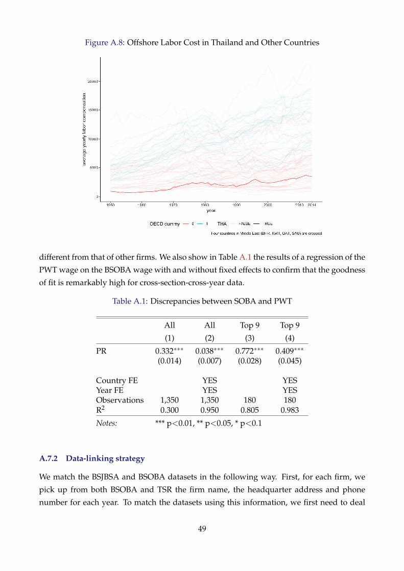
Figure A.8: Offshore Labor Cost in Thailand and Other Countries

different from that of other firms. We also show in Table A.1 the results of a regression of the

PWT wage on the BSOBA wage with and without fixed effects to confirm that the goodness

of fit is remarkably high for cross-section-cross-year data.

Table A.1: Discrepancies between SOBA and PWT

All All Top 9 Top 9

(1) (2) (3) (4)

PR 0.332∗∗∗ 0.038∗∗∗ 0.772∗∗∗ 0.409∗∗∗

(0.014) (0.007) (0.028) (0.045)

Country FE YES YESYear FE YES YESObservations 1,350 1,350 180 180R2 0.300 0.950 0.805 0.983

Notes: *** p<0.01, ** p<0.05, * p<0.1

A.7.2 Data-linking strategy

We match the BSJBSA and BSOBA datasets in the following way. First, for each firm, we

pick up from both BSOBA and TSR the firm name, the headquarter address and phone

number for each year. To match the datasets using this information, we first need to deal

49

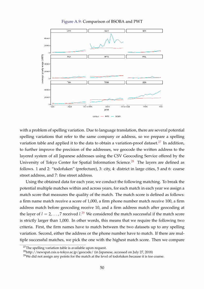
Figure A.9: Comparison of BSOBA and PWT

with a problem of spelling variation. Due to language translation, there are several potential

spelling variations that refer to the same company or address, so we prepare a spelling

variation table and applied it to the data to obtain a variation-proof dataset.27 In addition,

to further improve the precision of the addresses, we geocode the written address to the

layered system of all Japanese addresses using the CSV Geocoding Service offered by the

University of Tokyo Center for Spatial Information Science.28 The layers are defined as

follows. 1 and 2: “todofuken” (prefecture), 3: city, 4: district in large cities, 5 and 6: coarse

street address, and 7: fine street address.

Using the obtained data for each year, we conduct the following matching. To break the

potential multiple matches within and across years, for each match in each year we assign a

match score that measures the quality of the match. The match score is defined as follows:

a firm name match receive a score of 1,000, a firm phone number match receive 100, a firm

address match before geocoding receive 10, and a firm address match after geocoding at

the layer of l = 2, . . . , 7 received l.29 We considered the match successful if the match score

is strictly larger than 1,000. In other words, this means that we require the following two

criteria. First, the firm names have to match between the two datasets up to any spelling

variation. Second, either the address or the phone number have to match. If there are mul-

tiple successful matches, we pick the one with the highest match score. Then we compare

27The spelling variation table is available upon request.28http://newspat.csis.u-tokyo.ac.jp/geocode/ (in Japanese, accessed on July 27, 2018)29We did not assign any points for the match at the level of todofuken because it is too coarse.

50

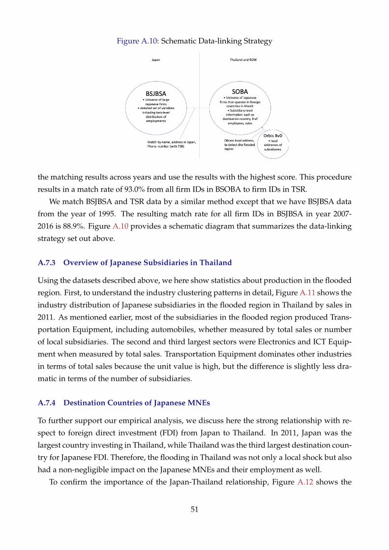
Figure A.10: Schematic Data-linking Strategy

the matching results across years and use the results with the highest score. This procedure

results in a match rate of 93.0% from all firm IDs in BSOBA to firm IDs in TSR.

We match BSJBSA and TSR data by a similar method except that we have BSJBSA data

from the year of 1995. The resulting match rate for all firm IDs in BSJBSA in year 2007-

2016 is 88.9%. Figure A.10 provides a schematic diagram that summarizes the data-linking

strategy set out above.

A.7.3 Overview of Japanese Subsidiaries in Thailand

Using the datasets described above, we here show statistics about production in the flooded

region. First, to understand the industry clustering patterns in detail, Figure A.11 shows the

industry distribution of Japanese subsidiaries in the flooded region in Thailand by sales in

2011. As mentioned earlier, most of the subsidiaries in the flooded region produced Trans-

portation Equipment, including automobiles, whether measured by total sales or number

of local subsidiaries. The second and third largest sectors were Electronics and ICT Equip-

ment when measured by total sales. Transportation Equipment dominates other industries

in terms of total sales because the unit value is high, but the difference is slightly less dra-

matic in terms of the number of subsidiaries.

A.7.4 Destination Countries of Japanese MNEs

To further support our empirical analysis, we discuss here the strong relationship with re-

spect to foreign direct investment (FDI) from Japan to Thailand. In 2011, Japan was the

largest country investing in Thailand, while Thailand was the third largest destination coun-

try for Japanese FDI. Therefore, the flooding in Thailand was not only a local shock but also

had a non-negligible impact on the Japanese MNEs and their employment as well.

To confirm the importance of the Japan-Thailand relationship, Figure A.12 shows the

51

Figure A.11: Industry Distribution of the Treated Subsidiaries of Japanese firms, 2011

(a) Total Sales (b) Number of Subsidiaries

Figure A.12: Top 10 Countries in which Japanese Firms Have Subsidiaries

(a) 2007 (b) 2016

top 10 countries in which Japanese firms had subsidiaries in 2007 and 2016. During these

10 years, the ranking of the top five countries did not change (China, U.S., Thailand, Hong

Kong, and Singapore), which indicates the stable economic relationship between these coun-

tries and Japanese firms. The number of Japanese firms with links to Thailand actually grew

during this period.

A.7.5 Balancing Analysis

To check the similarity between the firms that experienced and did not experience flood-

ing, we conduct several balancing tests. Figure A.13 shows the industry distribution of

subsidiary manufacturing firms for the group of parent firms that invested in 2011 in the

flooded region in Thailand (labeled Thai) and other regions of Thailand and the ROW (la-

beled Others).

Qualitatively, industries that had many firms in the flooded region of Thailand are likely

to also have had a higher number of firms in other countries, but the flooded region had rel-

52

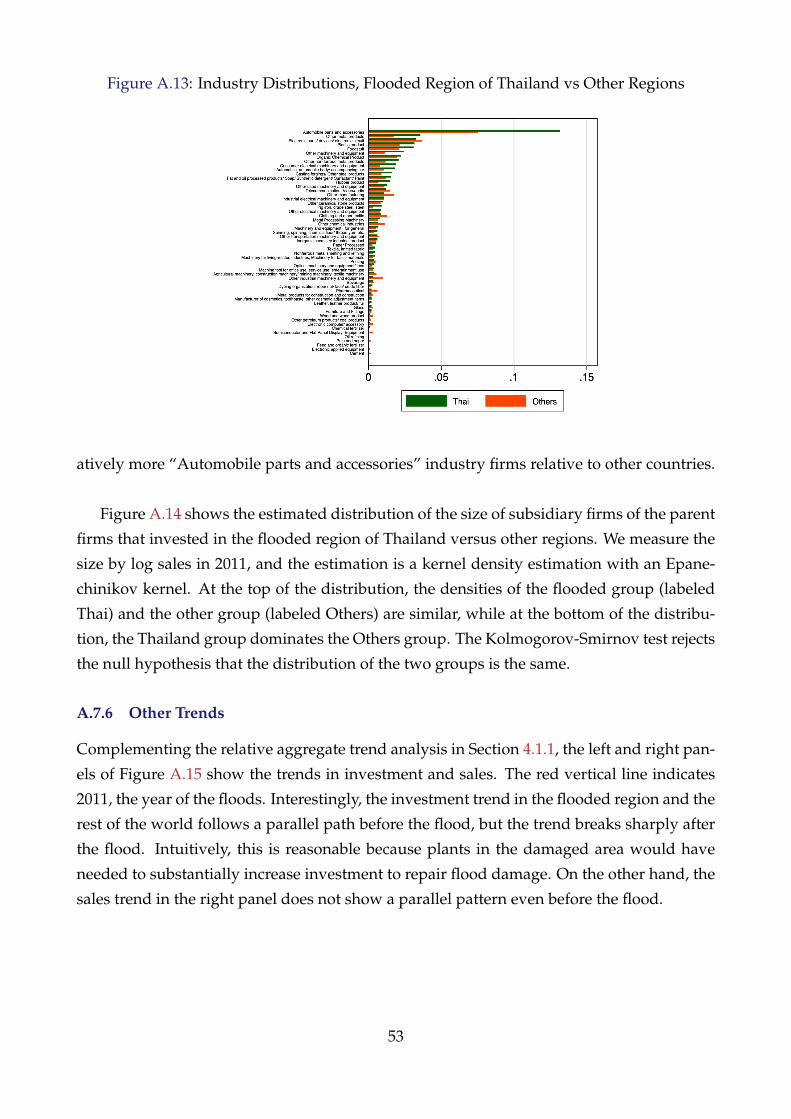
Figure A.13: Industry Distributions, Flooded Region of Thailand vs Other Regions

atively more “Automobile parts and accessories” industry firms relative to other countries.

Figure A.14 shows the estimated distribution of the size of subsidiary firms of the parent

firms that invested in the flooded region of Thailand versus other regions. We measure the

size by log sales in 2011, and the estimation is a kernel density estimation with an Epane-

chinikov kernel. At the top of the distribution, the densities of the flooded group (labeled

Thai) and the other group (labeled Others) are similar, while at the bottom of the distribu-

tion, the Thailand group dominates the Others group. The Kolmogorov-Smirnov test rejects

the null hypothesis that the distribution of the two groups is the same.

A.7.6 Other Trends

Complementing the relative aggregate trend analysis in Section 4.1.1, the left and right pan-

els of Figure A.15 show the trends in investment and sales. The red vertical line indicates

2011, the year of the floods. Interestingly, the investment trend in the flooded region and the

rest of the world follows a parallel path before the flood, but the trend breaks sharply after

the flood. Intuitively, this is reasonable because plants in the damaged area would have

needed to substantially increase investment to repair flood damage. On the other hand, the

sales trend in the right panel does not show a parallel pattern even before the flood.

53

Figure A.14: Sales Distributions, Flooded Region of Thailand vs Others

A.7.7 Choice of Treatment Groups

As described in Section 4.1.1, the flood severely affected Ayutthaya and Pathum Thani provinces.

However, it is important to acknowledge these particular provinces because Thailand over-

all was relatively unaffected in terms of employment or number of subsidiaries of Japanese

MNEs after the flood, as seen in Figure A.16, which shows the trends in employment

and number of Japanese subsidiaries inside and outside of Thailand instead of only in the

flooded provinces. One can see that the impact on total Thai employment and number of

subsidiaries is not as stark as when we compare the flooded provinces versus the rest of

the world in Figure 3. Therefore, in our main analysis, we take these two heavily flooded

provinces as the shocked regions and construct the IV based on that idea. Note again that,

for this purpose, it is critical to link our BSOBA data, which only contains the country infor-

mation of each Japanese MNE overseas factory, to Orbis BvD that contains specific factory

addresses.

A.8 Calibration Details

A.8.1 Estimation of σ

Following recent developments in estimating capital-labor elasticities (Oberfield and Raval,

2014; Raval, 2019), we estimate σ using the regression equation (20). Our coefficient of

interest is b1 since σ = b1 + 1.

To obtain the factor payment ratio (rk/wl)i, we use the annual Census of Manufacture

54

Figure A.15: Relative Trends in Investment and Sales of Japanese MNEs

(a) Investment (b) Sales

Figure A.16: Trends in Employment and Japanese MNE Subsidiaries, Thailand versus ROW

(a) Total employment (b) Count of subsidiaries

(CoM) survey. For our purposes, we use the initial stock of tangible assets in the next year

survey. To obtain the total payment to workers, we use the variable total payroll for all

workers, which includes both full-time and part-time workers. Since we can obtain the

rental rate of capital at the industry level, it drops with the industry-fixed effect in speci-

fication (20). Finally, CoM also offers municipality, 4-digit industry, and multiplant status

variables. The multiplant status includes three values: no other plants or headquarter office;

no other plant but a headquarter office; has other offices. We include the fixed effect for all

of these values in specification (20).

For the local wage, we use the municipality-level wage taken from the long-run eco-

nomic database of the Japan Cabinet Office. The long-run trend data offers the taxpayer-

per-capita taxable income from 1975 to 2013.30 The municipality unit is as of the last day of

April 2014. We convert the municipality code in each analysis year to the one as of April

30The primary data source of this dataset is the Survey of Municipality Taxation administered by Ministry ofInternal Affairs and Communications, Japan.

55

2014 using Municipality Map Maker (Kirimura et al., 2011).

To control the endogeneity in equation (20), we use a shift-share instrument (Bartik, 1991;

Goldsmith-Pinkham et al., 2018). Specifically, estimation equation (20) may be biased with

the existence of labor-augmenting productivity shocks to locality m (i). If m (i) receives

a positive shock, then wm(i) increases and (rK/wL)i decreases, so β would be negatively

biased. To obtain the exogenous shifter that changes wm(i) but not (rK/wL)i without the

influence through wm(i), we take the average of national growth in employment weighted

by the base-year employment share of non-manufacturing industries. In particular, from the

Employment Status Survey (ESS), we take the ten year growth in employment in industry n

as gn,t = ln (Ln,t/Ln,t−10) /10. We then take the base-year industry-n share of employment

ωm,n,t−10 in municipality m, and calculate our shift-share instrument by

zj,t = ∑n

ωm,n,t−10gn,t.

Table A.2 shows the results of regression (20) for 1997 since it is the nearest year to that

of the ESS survey.

56

Table A.2: Estimates of σ− 1

OLS, CO OLS, BSWS, all OLS, BSWS, manuf. IV, CO IV, BSWS, all IV, BSWS, manuf.log(wm(i)) −0.60∗∗∗ −0.20∗∗∗ −0.13∗∗∗ −1.15∗∗∗ −1.24∗∗∗ −0.88∗∗∗

(0.05) (0.04) (0.03) (0.18) (0.18) (0.13)Num. obs. 51477 51477 51477 51477 51477 51477

∗∗∗p < 0.001, ∗∗p < 0.01, ∗p < 0.05. CO indicates that the wage data is from the Cabinet Office. BSWS indicates that the wage data is from the Basic Survey of Wage Structures. ”BSWS, all” indicatesthat the wage variable is taken from all industries, while ”BSWS, manuf.” indicates that the wage variable is taken from manufacturing industries. See the text for detail. All regressions includeindustry FE and multiunit status indicator. Standard errors are clustered at municipality level.

57

Figure A.17: Distribution of Measured Markup m

Note: The authors’ computation from Census of Manufacture, 2011. Estimates are obtained by inverting themarkup, following Oberfield and Raval (2014). The markup is defined as sales divided by the sum of costsfrom capital, labor, and materials.

Comparison to the Literature The central estimate of Oberfield and Raval (2014) was

around 0.7. However, this value includes industry-level heterogeneity in substitutability

and the caused reallocation mechanism. Oberfield and Raval (2014) reports that plant-level

elasticity estimates range from 0.4-0.7 depending on the industry, which is closer to our

value. Incorporating heterogeneity into the model is our high-priority next research step.

Moreover, the capital-labor substitution parameters at micro and macro-level estimates

sometimes disagree. In fact, although microdata-based findings by ourselves and Oberfield

and Raval (2014) both point to gross-complementary capital and labor, the macro estimates

often indicate that they are gross substitutes (Karabarbounis and Neiman, 2013; Hubmer,

2018). Note that these macro estimates typically rely on U.S. data. In Japan, even at the

macro level, Hirakata and Koike (2018) show that the capital-labor elasticity is below one,

which is qualitatively consistent with our findings.

A.8.2 Detailed Results regarding ε and CSM

Figure A.17 shows the distribution of measured markups, which exhibits a spike at a value

slightly larger than one and a longer tail on the right side than the left. Our estimate ε = 4 is

based on the peak value of measured markup m = 4/3, which is standard in the literature

(Oberfield and Raval, 2014).

58

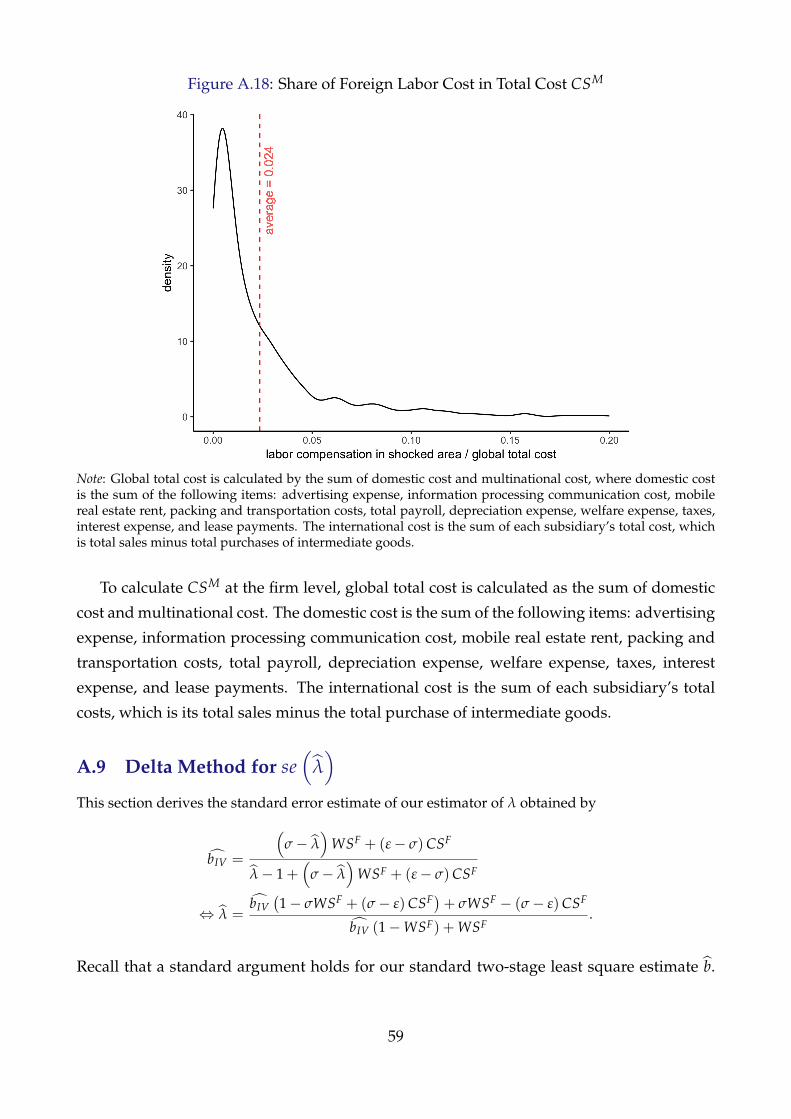
Figure A.18: Share of Foreign Labor Cost in Total Cost CSM

Note: Global total cost is calculated by the sum of domestic cost and multinational cost, where domestic costis the sum of the following items: advertising expense, information processing communication cost, mobilereal estate rent, packing and transportation costs, total payroll, depreciation expense, welfare expense, taxes,interest expense, and lease payments. The international cost is the sum of each subsidiary’s total cost, whichis total sales minus total purchases of intermediate goods.

To calculate CSM at the firm level, global total cost is calculated as the sum of domestic

cost and multinational cost. The domestic cost is the sum of the following items: advertising

expense, information processing communication cost, mobile real estate rent, packing and

transportation costs, total payroll, depreciation expense, welfare expense, taxes, interest

expense, and lease payments. The international cost is the sum of each subsidiary’s total

costs, which is its total sales minus the total purchase of intermediate goods.

A.9 Delta Method for se(

λ)

This section derives the standard error estimate of our estimator of λ obtained by

bIV =

(σ− λ

)WSF + (ε− σ)CSF

λ− 1 +(

σ− λ)

WSF + (ε− σ)CSF

⇔ λ =bIV(1− σWSF + (σ− ε)CSF)+ σWSF − (σ− ε)CSF

bIV (1−WSF) + WSF.

Recall that a standard argument holds for our standard two-stage least square estimate b.

59

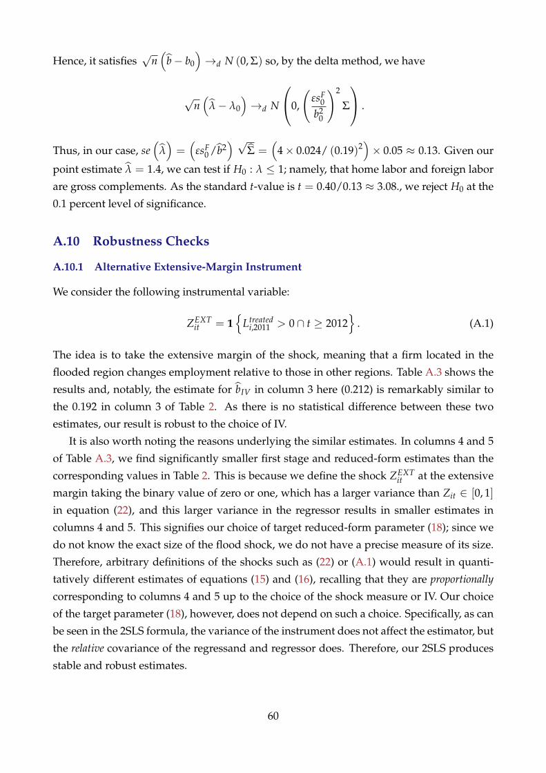
Hence, it satisfies√

n(

b− b0

)→d N (0, Σ) so, by the delta method, we have

√n(

λ− λ0

)→d N

0,

(εsF

0

b20

)2

Σ

.

Thus, in our case, se(

λ)=(

εsF0 /b2

) √Σ =

(4× 0.024/ (0.19)2

)× 0.05 ≈ 0.13. Given our

point estimate λ = 1.4, we can test if H0 : λ ≤ 1; namely, that home labor and foreign labor

are gross complements. As the standard t-value is t = 0.40/0.13 ≈ 3.08., we reject H0 at the

0.1 percent level of significance.

A.10 Robustness Checks

A.10.1 Alternative Extensive-Margin Instrument

We consider the following instrumental variable:

ZEXTit = 1

{Ltreated

i,2011 > 0∩ t ≥ 2012}

. (A.1)

The idea is to take the extensive margin of the shock, meaning that a firm located in the

flooded region changes employment relative to those in other regions. Table A.3 shows the

results and, notably, the estimate for bIV in column 3 here (0.212) is remarkably similar to

the 0.192 in column 3 of Table 2. As there is no statistical difference between these two

estimates, our result is robust to the choice of IV.

It is also worth noting the reasons underlying the similar estimates. In columns 4 and 5

of Table A.3, we find significantly smaller first stage and reduced-form estimates than the

corresponding values in Table 2. This is because we define the shock ZEXTit at the extensive

margin taking the binary value of zero or one, which has a larger variance than Zit ∈ [0, 1]

in equation (22), and this larger variance in the regressor results in smaller estimates in

columns 4 and 5. This signifies our choice of target reduced-form parameter (18); since we

do not know the exact size of the flood shock, we do not have a precise measure of its size.

Therefore, arbitrary definitions of the shocks such as (22) or (A.1) would result in quanti-

tatively different estimates of equations (15) and (16), recalling that they are proportionally

corresponding to columns 4 and 5 up to the choice of the shock measure or IV. Our choice

of the target parameter (18), however, does not depend on such a choice. Specifically, as can

be seen in the 2SLS formula, the variance of the instrument does not affect the estimator, but

the relative covariance of the regressand and regressor does. Therefore, our 2SLS produces

stable and robust estimates.

60

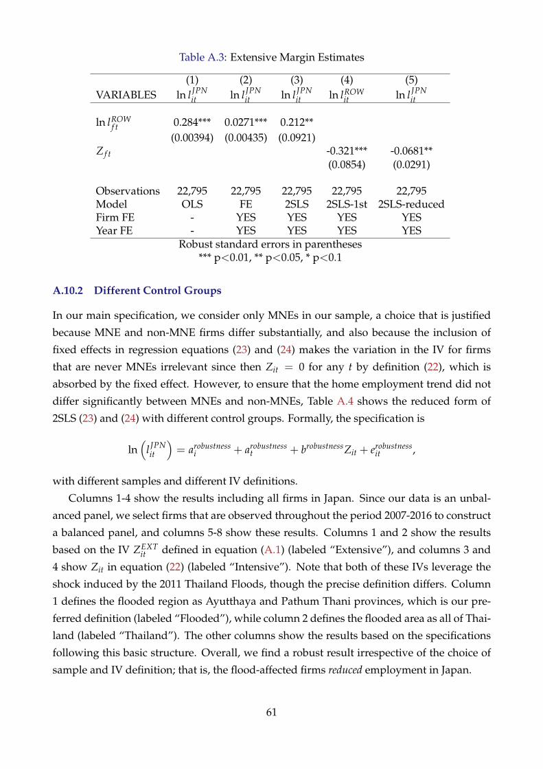
Table A.3: Extensive Margin Estimates

(1) (2) (3) (4) (5)VARIABLES ln l JPN

it ln l JPNit ln l JPN

it ln lROWit ln l JPN

it

ln lROWf t 0.284*** 0.0271*** 0.212**

(0.00394) (0.00435) (0.0921)Z f t -0.321*** -0.0681**

(0.0854) (0.0291)

Observations 22,795 22,795 22,795 22,795 22,795Model OLS FE 2SLS 2SLS-1st 2SLS-reducedFirm FE - YES YES YES YESYear FE - YES YES YES YES

Robust standard errors in parentheses*** p<0.01, ** p<0.05, * p<0.1

A.10.2 Different Control Groups

In our main specification, we consider only MNEs in our sample, a choice that is justified

because MNE and non-MNE firms differ substantially, and also because the inclusion of

fixed effects in regression equations (23) and (24) makes the variation in the IV for firms

that are never MNEs irrelevant since then Zit = 0 for any t by definition (22), which is

absorbed by the fixed effect. However, to ensure that the home employment trend did not

differ significantly between MNEs and non-MNEs, Table A.4 shows the reduced form of

2SLS (23) and (24) with different control groups. Formally, the specification is

ln(

l JPNit

)= arobustness

i + arobustnesst + brobustnessZit + erobustness

it ,

with different samples and different IV definitions.

Columns 1-4 show the results including all firms in Japan. Since our data is an unbal-

anced panel, we select firms that are observed throughout the period 2007-2016 to construct

a balanced panel, and columns 5-8 show these results. Columns 1 and 2 show the results

based on the IV ZEXTit defined in equation (A.1) (labeled “Extensive”), and columns 3 and

4 show Zit in equation (22) (labeled “Intensive”). Note that both of these IVs leverage the

shock induced by the 2011 Thailand Floods, though the precise definition differs. Column

1 defines the flooded region as Ayutthaya and Pathum Thani provinces, which is our pre-

ferred definition (labeled “Flooded”), while column 2 defines the flooded area as all of Thai-

land (labeled “Thailand”). The other columns show the results based on the specifications

following this basic structure. Overall, we find a robust result irrespective of the choice of

sample and IV definition; that is, the flood-affected firms reduced employment in Japan.

61

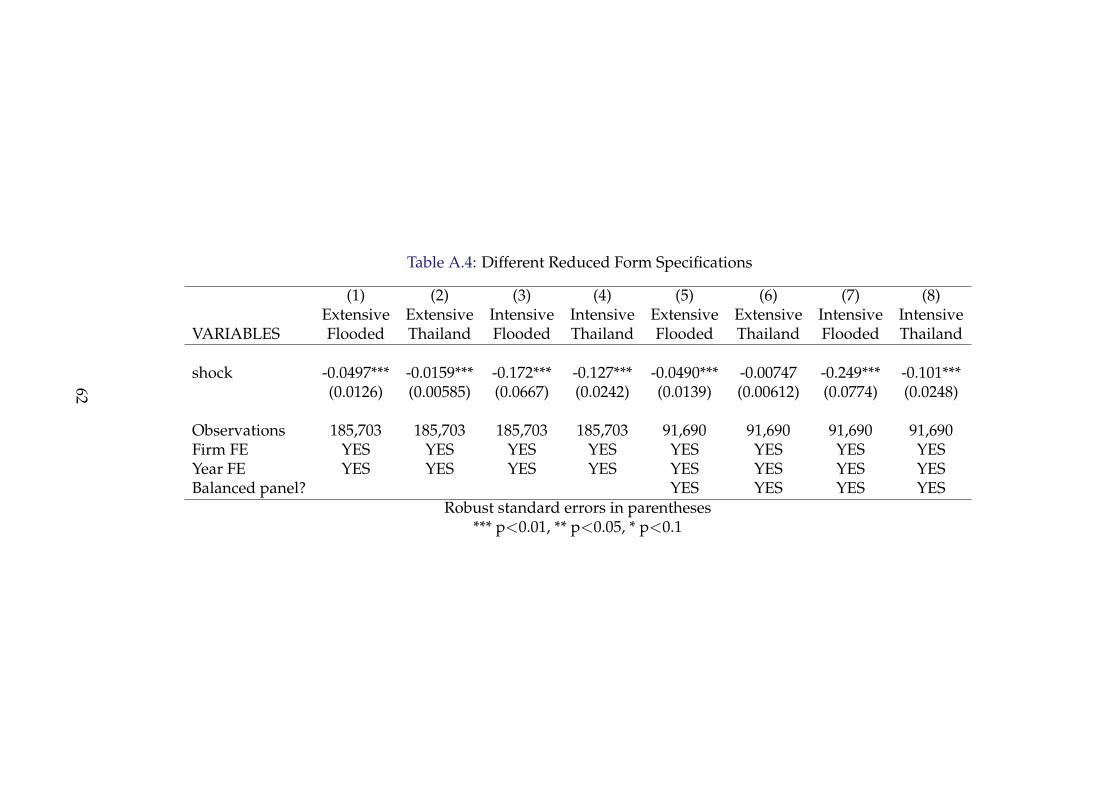
Table A.4: Different Reduced Form Specifications

(1) (2) (3) (4) (5) (6) (7) (8)Extensive Extensive Intensive Intensive Extensive Extensive Intensive Intensive

VARIABLES Flooded Thailand Flooded Thailand Flooded Thailand Flooded Thailand

shock -0.0497*** -0.0159*** -0.172*** -0.127*** -0.0490*** -0.00747 -0.249*** -0.101***(0.0126) (0.00585) (0.0667) (0.0242) (0.0139) (0.00612) (0.0774) (0.0248)

Observations 185,703 185,703 185,703 185,703 91,690 91,690 91,690 91,690Firm FE YES YES YES YES YES YES YES YESYear FE YES YES YES YES YES YES YES YESBalanced panel? YES YES YES YES

Robust standard errors in parentheses*** p<0.01, ** p<0.05, * p<0.1

62

Indeed, it is crucial to have the IV defined according to the flood-induced variation,

despite minor differences in definitions between equations (22) and (A.1). In Section A.11.1,

we see that another widely-used IV definition, the Bartik instrument, does not work in

our context, which highlights our choice based on the natural experiment and its power of

identification.

A.10.3 The 2011 Tohoku Earthquake

As another check of the robustness of our results, we now consider the potential impact

on our results of the 2011 Tohoku Earthquake, another severe natural disaster that affected

Japanese industry that year. It’s impact on the country was so profound that it remains in

the minds of Japanese today almost a decade later. Carvalho et al. (2016) summarizes the

event as follows: “On March 11, 2011, a magnitude 9.0 earthquake occurred off the northeast

coast of Japan. This was the largest earthquake in the history of Japan and the fifth largest

in the world since 1900. The earthquake brought a three-fold impact on the residents of

northeast Japan: (i) the main earthquake and its aftershocks, directly responsible for much

of the material damage that ensued; (ii) the resulting tsunami, which flooded 561 square

kilometers of the northeast coastline; and (iii) the failure of the Fukushima Dai-ichi Nuclear

Power Plant that led to the evacuation of 99,000 residents of the Fukushima prefecture.”

Since our data is annual and the flooding in Thailand began about four months after the

earthquake in Japan, we want to ensure that our results using the Thai Floods as a natu-

ral experiment are not qualitatively affected by the co-ocurrence of the Tohoku earthquake

that same year. There are two ways to address this concern. First, our specifications (23)

and (24) include the fixed effects of firms, which means that we are leveraging the varia-

tion within a firm across years, not the differences between firms that may or may not have

experienced the earthquake. Second, in order to further mitigate any concern that the exis-

tence of flooded firms in the main sample still biases the fixed effect estimator, we conduct

the following robustness check exercise. We drop firms located in the four most severely hit

prefectures in Japan–Aomori, Iwate, Miyagi, and Fukushima (called “damaged prefectures”

below). These damaged prefectures include 36 municipalities that were designated as dis-

aster areas by the Ministry of Land, Infrastructure, Transport and Tourism (MLIT) of Japan

after the earthquake, and this is also used by Carvalho et al. (2016), which an interested

reader may refer to for the rationale.31

31Although the propagation of the shock due to the input-output linkages makes it not trivial to measurethe exact impact of the earthquake on each firm, we view our choice as a conservative test for the existence ofan earthquake effect on our estimator. Namely, since the firms located in the defined four prefectures sufferedmost from the earthquake, if there are any confounding effects of the earthquake on our estimator, droppingsuch firms should substantially alter the estimate. Thus, if we find no difference between our full sampleand the sample omitting these four prefectures, this indicates that any potential earthquake effects are notsignificant.

63

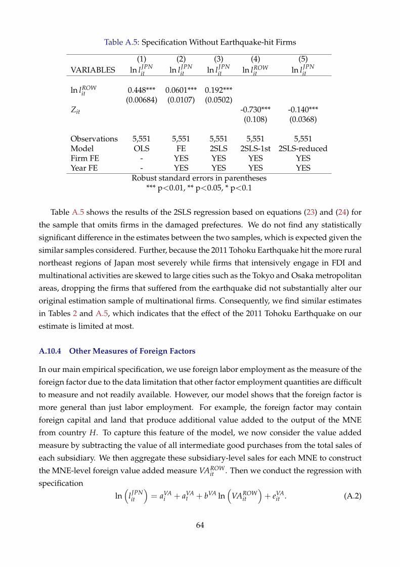
Table A.5: Specification Without Earthquake-hit Firms

(1) (2) (3) (4) (5)VARIABLES ln l JPN

it ln l JPNit ln l JPN

it ln lROWit ln l JPN

it

ln lROWit 0.448*** 0.0601*** 0.192***

(0.00684) (0.0107) (0.0502)Zit -0.730*** -0.140***

(0.108) (0.0368)

Observations 5,551 5,551 5,551 5,551 5,551Model OLS FE 2SLS 2SLS-1st 2SLS-reducedFirm FE - YES YES YES YESYear FE - YES YES YES YES

Robust standard errors in parentheses*** p<0.01, ** p<0.05, * p<0.1

Table A.5 shows the results of the 2SLS regression based on equations (23) and (24) for

the sample that omits firms in the damaged prefectures. We do not find any statistically

significant difference in the estimates between the two samples, which is expected given the

similar samples considered. Further, because the 2011 Tohoku Earthquake hit the more rural

northeast regions of Japan most severely while firms that intensively engage in FDI and

multinational activities are skewed to large cities such as the Tokyo and Osaka metropolitan

areas, dropping the firms that suffered from the earthquake did not substantially alter our

original estimation sample of multinational firms. Consequently, we find similar estimates

in Tables 2 and A.5, which indicates that the effect of the 2011 Tohoku Earthquake on our

estimate is limited at most.

A.10.4 Other Measures of Foreign Factors

In our main empirical specification, we use foreign labor employment as the measure of the

foreign factor due to the data limitation that other factor employment quantities are difficult

to measure and not readily available. However, our model shows that the foreign factor is

more general than just labor employment. For example, the foreign factor may contain

foreign capital and land that produce additional value added to the output of the MNE

from country H. To capture this feature of the model, we now consider the value added

measure by subtracting the value of all intermediate good purchases from the total sales of

each subsidiary. We then aggregate these subsidiary-level sales for each MNE to construct

the MNE-level foreign value added measure VAROWit . Then we conduct the regression with

specification

ln(

l JPNit

)= aVA

i + aVAt + bVA ln

(VAROW

it

)+ eVA

it . (A.2)

64

Table A.6: VA-based Regressor with IV (22)

(1) (2) (3) (4) (5)VARIABLES ln VAROW

it ln l JPNit ln l JPN

it ln salesROWit ln l JPN

it

Zit -0.762*** -0.132*** -0.549***(0.105) (0.0374) (0.0849)

ln(VAROWit ) 0.173***

(0.0494)ln(salesROW

it ) 0.240***(0.0685)

Observations 5,460 5,460 5,460 5,460 5,460Model 2SLS-1st 2SLS-reduced 2SLS 2SLS-1st 2SLSFirm FE YES YES YES YES YESYear FE YES YES YES YES YES

Robust standard errors in parentheses*** p<0.01, ** p<0.05, * p<0.1

As an additional check, we also substitute a raw sales measure for the value added measure.

Here, we construct the flood shock-based IV as in the main text, but with our value added

measure instead:

ZVAit =

VA f loodedi,2011

VAJPNi,2011 + VAROW

i,2011

× 1 {t ≥ 2012} . (A.3)

Since both IVs (22) and (A.3) satisfy the standard requirements for IVs under our maintained

assumption that the flood was an unexpected augmentation shock to the MNEs located in

the damaged region, we conduct the robustness exercise based on both definitions.

Tables A.6 and A.7 show the results from our VA-based regressor specification (A.2)

using our preferred IV (22) and the IV defined by equation (A.3), respectively. Both tables

share the same structure; Columns 1-3 show the results using VAROWit as the regressor, while

columns 4 and 5 use the raw sales measure. Columns 1 and 4 show the first stage results

to check the relevance of the IV, and column 2 shows the reduced form relating the IV

to the outcome variable. Note that the value added and crude sales regressors share the

same reduced form. Finally, columns 3 and 5 show the 2SLS results, and particularly worth

mentioning is that they are all qualitatively similar no matter what regressors and IVs were

used. Therefore, we view our preferred result reported in Table 2 as robust to the choice

both of variables for foreign factor employment and IVs.

A.10.5 Long-difference Specification

Our main empirical specification (23) and (24) is meant to identify the medium- to long-

run elasticity for five years after the flood. Another way to approach this is to conduct a

65

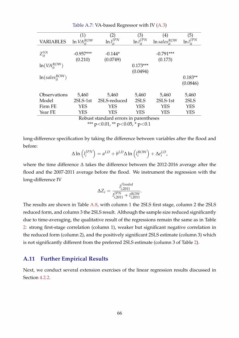
Table A.7: VA-based Regressor with IV (A.3)

(1) (2) (3) (4) (5)VARIABLES ln VAROW

it ln l JPNit ln l JPN

it ln salesROWit ln l JPN

it

ZVAit -0.957*** -0.144* -0.791***

(0.210) (0.0749) (0.173)ln(VAROW

it ) 0.173***(0.0494)

ln(salesROWit ) 0.183**

(0.0846)

Observations 5,460 5,460 5,460 5,460 5,460Model 2SLS-1st 2SLS-reduced 2SLS 2SLS-1st 2SLSFirm FE YES YES YES YES YESYear FE YES YES YES YES YES

Robust standard errors in parentheses*** p<0.01, ** p<0.05, * p<0.1

long-difference specification by taking the difference between variables after the flood and

before:

∆ ln(

l JPNi

)= aLD + bLD∆ ln

(lROWi

)+ ∆eLD

i ,

where the time difference ∆ takes the difference between the 2012-2016 average after the

flood and the 2007-2011 average before the flood. We instrument the regression with the

long-difference IV

∆Zi =l f loodedi,2011

l JPNi,2011 + lROW

i,2011

.

The results are shown in Table A.8, with column 1 the 2SLS first stage, column 2 the 2SLS

reduced form, and column 3 the 2SLS result. Although the sample size reduced significantly

due to time-averaging, the qualitative result of the regressions remain the same as in Table

2: strong first-stage correlation (column 1), weaker but significant negative correlation in

the reduced form (column 2), and the positively significant 2SLS estimate (column 3) which

is not significantly different from the preferred 2SLS estimate (column 3 of Table 2).

A.11 Further Empirical Results

Next, we conduct several extension exercises of the linear regression results discussed in

Section 4.2.2.

66

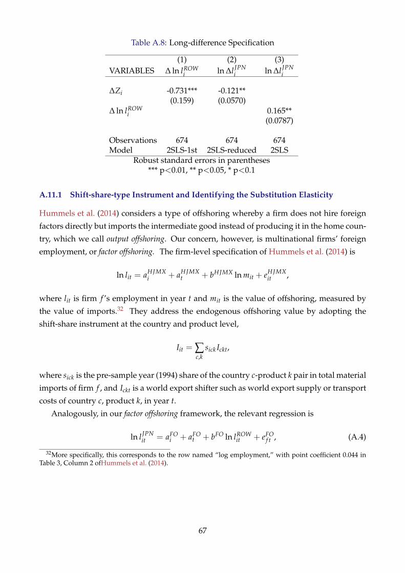
Table A.8: Long-difference Specification

(1) (2) (3)VARIABLES ∆ ln lROW

i ln ∆l JPNi ln ∆l JPN

i

∆Zi -0.731*** -0.121**(0.159) (0.0570)

∆ ln lROWi 0.165**

(0.0787)

Observations 674 674 674Model 2SLS-1st 2SLS-reduced 2SLS

Robust standard errors in parentheses*** p<0.01, ** p<0.05, * p<0.1

A.11.1 Shift-share-type Instrument and Identifying the Substitution Elasticity

Hummels et al. (2014) considers a type of offshoring whereby a firm does not hire foreign

factors directly but imports the intermediate good instead of producing it in the home coun-

try, which we call output offshoring. Our concern, however, is multinational firms’ foreign

employment, or factor offshoring. The firm-level specification of Hummels et al. (2014) is

ln lit = aHJMXi + aHJMX

t + bHJMX ln mit + eHJMXit ,

where lit is firm f ’s employment in year t and mit is the value of offshoring, measured by

the value of imports.32 They address the endogenous offshoring value by adopting the

shift-share instrument at the country and product level,

Iit = ∑c,k

sick Ickt,

where sick is the pre-sample year (1994) share of the country c-product k pair in total material

imports of firm f , and Ickt is a world export shifter such as world export supply or transport

costs of country c, product k, in year t.

Analogously, in our factor offshoring framework, the relevant regression is

ln l JPNit = aFO

i + aFOt + bFO ln lROW

it + eFOf t , (A.4)

32More specifically, this corresponds to the row named “log employment,” with point coefficient 0.044 inTable 3, Column 2 ofHummels et al. (2014).

67

where lROWit is employment of offshore workers and the instrument is

IROWit = ∑

csO

ic LROWct ,

where sOc is the pre-sample year (in our case, 2007) share of offshore employment in country

c of firm i, and empO,−JPNct is the stock of workers at subsidiaries of multinational firms

excluding those in Japan. However, as we do not find a relevant measure for LROWct , we

need a proxy for that.

Note that Desai et al. (2009) takes the GDP growth rate in each country as the instru-

mental variable, based on the idea that “national economic growth is associated with pro-

ductivity gains that correspond to declining real input costs” (p. 186). A problem that one

can imagine with this proxy is that the GDP growth rate does not necessarily reflect the

offshorability or availability of offshore factors in the destination country. For example,

the GDP growth rate might not reflect political instability (Pierce and Schott, 2016). If a

country has high growth but high political instability that makes employment difficult for

multinational firms, then GDP growth might overstate the actual ability to offshore in the

country. Moreover, the Desai et al. (2009) measure is the GDP growth rate rather than the

level of GDP, whereas Hummels et al. (2014) take world trade value levels to construct the

instrumental variable. With these cautions in mind, we calculate the instrumental variable

as follows:

IROWit = ∑

csO

ic gct,

where gct is the GDP growth rate of country c from year t− 1 to year t.

While Hummels et al. (2014) find a statistically significant substitution of home labor

with the foreign imported intermediate input, in contrast, we do not find a similar substi-

tution result (Table A.9). This highlights the difficulty in using a Bartik-type instrument to

identify the effect of factor-usage offshorability on home employment, as we emphasized in

the beginning of Section 4.

68

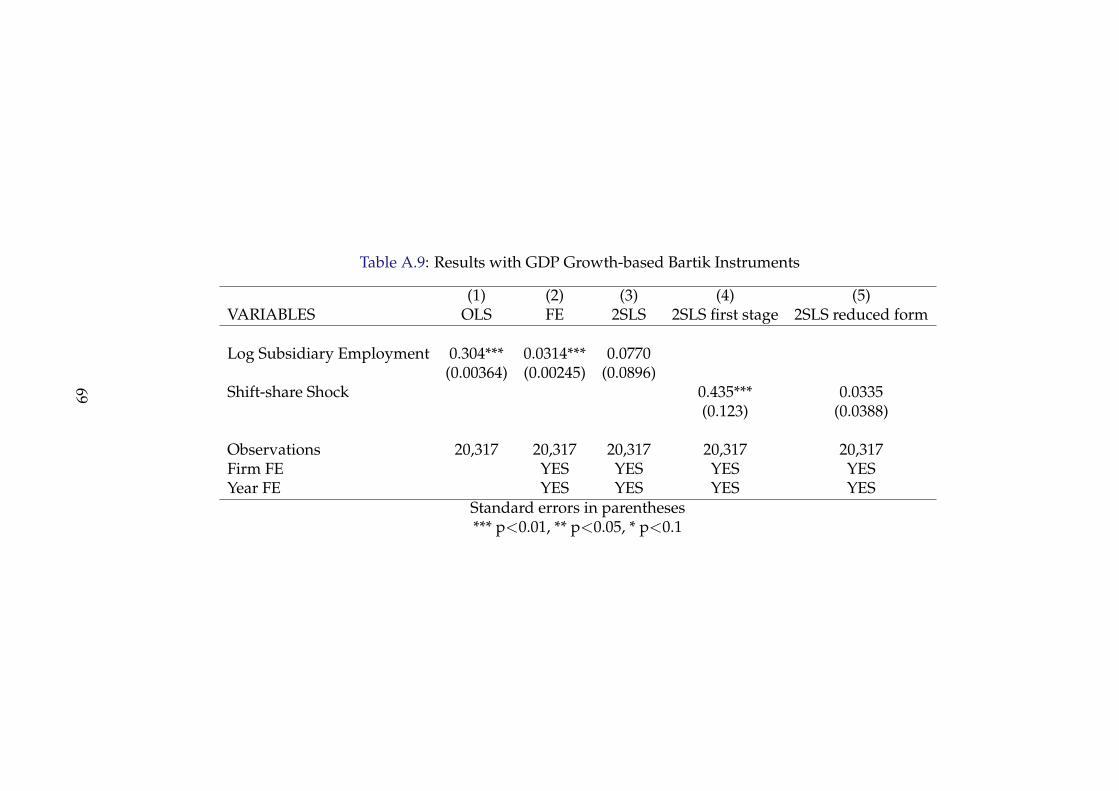
Table A.9: Results with GDP Growth-based Bartik Instruments

(1) (2) (3) (4) (5)VARIABLES OLS FE 2SLS 2SLS first stage 2SLS reduced form

Log Subsidiary Employment 0.304*** 0.0314*** 0.0770(0.00364) (0.00245) (0.0896)

Shift-share Shock 0.435*** 0.0335(0.123) (0.0388)

Observations 20,317 20,317 20,317 20,317 20,317Firm FE YES YES YES YESYear FE YES YES YES YES

Standard errors in parentheses*** p<0.01, ** p<0.05, * p<0.1

69

Figure A.19: Results of Event Study Regression on Foreign Employment

(a) ∑l,JPN Llf t (b) Ltreated

f t

A.11.2 Long-run Impact on Foreign Employment

In our main specification (23) and (24), we consider the average long-run, but not time-

varying, impacts. As we saw in Figure 3, the flood had long-lasting effects on employment

in Thailand, so to see if this is true at the firm-level of those affected by the flood, we consider

the following event-study regression:

yit = aESi + aES

t + ∑τ,2011

bESτ

l f loodedi,2011

l JPNi,2011 + lROW

i,2011

× 1 {t = τ}+ eESit . (A.5)

Figure A.19 shows the event-study plots of bESt ,which confirm that the effect of the flood

persisted for at least five years in terms of foreign employment.

We next turn to the long-run effect on Home employment. Namely, we take log em-

ployment in Japan as yit and run regression (A.5), with the results shown in Figure A.20.

Consistent with the reduced form results of our main specification in Table 2, we find sig-

nificantly negative effects four years after the flood at the 5 percent significance level. We

can also confirm that the pre-trends are balanced since no coefficient before the year of the

flood is statistically significantly different from zero. In 2016, the coefficient is negative but

only marginally different from zero (significant only at the 10 percent level). This reversion

to zero may imply recovery from the flood for the firms that were severely hit. However,

even in the Home country (Japan), the recovery in terms of employment took at least five

years after the flood. In a nutshell, the event-study analysis supports our interpretation of

the shock as having a medium-run impact on worldwide factor employment by affected

firms.

70

Figure A.20: Results of Event Study Regression on Home Employment

Figure A.21: Growth in Sales Across Firms Located in Thailand in 2011 or Not

A.11.3 Third Country Substitution

Where do subsidiaries substitute production after the flood? To answer this in a brief man-

ner, we can observe the sales growth of subsidiaries in nearby countries (Indonesia, Laos,

Malaysia, Philippines, and Vietnam) between 2011 and 2012 for those firms affected and

unaffected by the flooding. If production substitution occurred in nearby countries, then

the MNEs affected by the floods would increase sales in nearby countries relative to un-

affected MNEs. Figure A.21 shows the sales growth rates of foreign subsidiaries in each

country near Thailand for those MNEs with subsidiaries in Thailand (labeled as “suffered”)

and those without (labeled as “not suffered”). As one can see, for all countries except Laos,

there is no relative increase in sales for firms hit by the flooding. Therefore, on average,

production substitution to nearby countries did not occur very strongly, which supports the

validity of our main analysis of production substitution between Japan and Thailand.

To more formally and systematically study the substitution after the flood, we conduct

the same regression specification as in the main text with a modified coefficient notation to

71

Table A.10: Third Country Substitution

(1) (2) (3) (4)VARIABLES ln empSEA

it ln empWorldit ln salesSEA

it ln salesWorldit

Zit 0.443 -1.039*** -0.600** -0.951***(0.354) (0.270) (0.253) (0.184)

Observations 2,434 5,549 2,364 5,489Firm FE YES YES YES YESYear FE YES YES YES YES

Robust standard errors in parentheses*** p<0.01, ** p<0.05, * p<0.1

indicate Third Country Substitution (TCS):

yit = aTCSi + aTCS

t + bTCSZit + eTCSit , (A.6)

and also with the outcome variable about operations in third countries. Specifically, we

take as an outcome variable log employment in Southeast Asian countries other than Thai-

land (Myanmar, Malaysia, Singapore, Indonesia, Phillipines, Cambodia, Laos, with notation

empSEAit ), log employment in the world other than in Thailand and Japan (empWorld

it ), log

sales in Southeast Asian countries other than Thailand (salesSEAit ), and log sales in the world

other than in Thailand and Japan (salesWorldit ). To best control any unobserved subsidiary

heterogeneity, we restrict the sample to subsidiaries located in Thailand, and compare the

headquarters that have subsidiaries in the flooded regions versus those that do not, using

our IV Zit. If third country substitution were significant, we would observe the positive

coefficient bTCS > 0.

Table A.10 shows the results of regression (A.6), and throughout columns 1-4, we do not

find positive substitution from the flooded regions to non-flooded third countries. Perhaps

surprisingly, we do find some strong negative effects on third country employment and sales.

In fact, this is consistent with our interpretation that the flood decreased overall productivity

of the affected MNEs, so that they decreased factor employment and sales everywhere in the

world, including third countries and Japan. Recall that this productivity effect could be seen

in our main regression result 2.

A.11.4 Regression by Industries

Table A.11 shows the results of the headquarter industry-regression for specification (22)

and (A.1), with panel A.11a showing the 2SLS results and A.12b and A.12c showing the cor-

responding first stage and reduced-form regressions. In each panel, column 1 refers to the

72

aggregated manufacturing sector and columns 2-6 the Chemical, Metal, General Machinery,

Electronic Machinery, and Automobile industries, respectively.

B Theory Appendix

This appendix provides proofs and extensions of the model described in Section 3.

B.1 Uniqueness of the Equilibrium

A desirable property of a general equilibrium is its uniqueness, as uniqueness guarantees

that the equilibrium is robust across shocks and parameter values. Although it is well-

known that the uniqueness result is difficult to obtain (Sonnenschein, 1972; Mantel, 1974;

Debreu, 1974), our constant returns to scale model allows us to adopt the generic uniqueness

approach described in Chapter 17 of Mas-Colell et al. (1995). In the explanation below,

proposition numbers that begin with “17” are all taken from that chapter.

We begin with the following facts: (i) Under a regularity condition, any equilibrium

factor price vector (r, w) is locally isolated (Proposition 17.D.1) and, furthermore, the reg-

ularity condition holds generically (Proposition 17.D.5); (ii) If the weak axiom of revealed

preference (WARP) is satisfied, then under constant returns to scale technology, the set of

equilibrium price vectors (r, w) is convex (Proposition 17.F.2). Note that as our factor de-

mand functions are obtained by solving a cost-minimization problem, so they satisfy WARP.

Thus, the set of equilibrium factor price vectors is both locally isolated convex and a single-

ton. Thus, we may conclude the following:

Proposition 1. (Generic Uniqueness) The general equilibrium defined in Section 3.1 is generically

unique.

B.2 Equivalence Results

We consider a special case of our model within offshoring and multinational models, begin-

ning the equilibrium analysis from modified versions of Feenstra and Hanson (1997) and

Arkolakis et al. (2017) to arrive at equation (6).

B.2.1 Offshoring

First, we propose a modified version of Feenstra and Hanson (1997) in which we do not

distinguish between high-skill and low-skill workers but we do distinguish between factor

augmenting productivity shocks in the Home country H and the Foreign country F. Each

country c = H, F is endowed with (Lc, Kc), and the factor prices are (wc, rc). Competitive

73

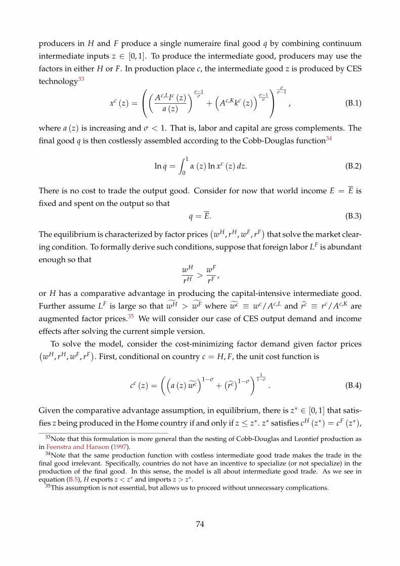
producers in H and F produce a single numeraire final good q by combining continuum

intermediate inputs z ∈ [0, 1]. To produce the intermediate good, producers may use the

factors in either H or F. In production place c, the intermediate good z is produced by CES

technology33

xc (z) =

(Ac,Llc (z)a (z)

) σ−1σ

+(

Ac,Kkc (z)) σ−1

σ

σσ−1

, (B.1)

where a (z) is increasing and σ < 1. That is, labor and capital are gross complements. The

final good q is then costlessly assembled according to the Cobb-Douglas function34

ln q =∫ 1

0α (z) ln xc (z) dz. (B.2)

There is no cost to trade the output good. Consider for now that world income E = E is

fixed and spent on the output so that

q = E. (B.3)

The equilibrium is characterized by factor prices(wH, rH, wF, rF) that solve the market clear-

ing condition. To formally derive such conditions, suppose that foreign labor LF is abundant

enough so thatwH

rH >wF

rF ,

or H has a comparative advantage in producing the capital-intensive intermediate good.

Further assume LF is large so that wH > wF where wc ≡ wc/Ac,L and rc ≡ rc/Ac,K are

augmented factor prices.35 We will consider our case of CES output demand and income

effects after solving the current simple version.

To solve the model, consider the cost-minimizing factor demand given factor prices(wH, rH, wF, rF). First, conditional on country c = H, F, the unit cost function is

cc (z) =((

a (z) wc)1−σ

+(rc)1−σ

) 11−σ

. (B.4)

Given the comparative advantage assumption, in equilibrium, there is z∗ ∈ [0, 1] that satis-

fies z being produced in the Home country if and only if z ≤ z∗. z∗ satisfies cH (z∗) = cF (z∗),

33Note that this formulation is more general than the nesting of Cobb-Douglas and Leontief production asin Feenstra and Hanson (1997).

34Note that the same production function with costless intermediate good trade makes the trade in thefinal good irrelevant. Specifically, countries do not have an incentive to specialize (or not specialize) in theproduction of the final good. In this sense, the model is all about intermediate good trade. As we see inequation (B.5), H exports z < z∗ and imports z > z∗.

35This assumption is not essential, but allows us to proceed without unnecessary complications.

74

or (a (z∗) wH

)1−σ+(

rH)1−σ

=(

a (z∗) wF)1−σ

+(

rF)1−σ

. (B.5)

The marginal cost is thus c (z) ≡ minc {cc (z)}. Given such z∗, by Shepherd’s lemma, the

factor demands are characterized by

lc (z) =

(a (z) wc

cc (z)

)−σ

a (z) xc (z) , (B.6)

kc (z) =

(rc

cc (z)

)−σ

xc (z) (B.7)

for c = H, F, where lc (z) ≡ Ac,Llc (z) and kc (z) ≡ Ac,Kkc (z) are the augmented factor

demands for variety z in country c. Hence, the market clearing conditions are

LH =∫ z∗

0lH (z) dz, (B.8)

KH =∫ z∗

0kH (z) dz, (B.9)

LF =∫ 1

z∗lF (z) dz, (B.10)

KF =∫ 1

z∗kF (z) dz, (B.11)

where Lc ≡ Ac,LLc and Kc ≡ Ac,KKc are the augmented endowments for c = H, F. To solve

xc (z), by Cobb-Douglas assumption (B.2), we have p (z) xc (z) = α (z) q, where p (z) is the

price of the intermediate good z. Moreover, the perfect competition assumption implies

that p (z) is given by the (minimum) marginal cost c (z). Thus, by good market clearing

condition (B.3), we have

xc (z) =α (z)c (z)

E. (B.12)

Thus, the equilibrium is(

z∗,(

wc, rc)

c∈(H,F)

)that solves equations (B.5), (B.8), (B.9),

(B.10), and (B.11). To study the Home labor share, we still have LS ≡ wH LH/(wH LH + rHKH)

that is to the first order

dLS = LS0 (1− LS0)(

d ln wH − d ln rH)

.

Hence, it remains to study d ln wH and d ln rH. For this purpose, we have log first-order

75

approximations with respect to d ln AF,L and d ln AF,K to equations (B.5), (B.8), (B.9), (B.10),

and (B.11) as follows:

CSH,L (z∗)(

σazd ln z∗ + d ln wH)+ CSH,K (z∗) d ln rH

= CSF,L (z∗)(

σazd ln z∗ + d ln wF)+ CSF,K (z∗) d ln rF

, (B.13)

0 =z∗ lH (z∗)

LHd ln z∗ − σd ln wH +

∫ z∗

0

lH (z)

LH

(σd ln cH (z) + d ln xH (z)

)dz,

0 =z∗kH (z∗)

KHd ln z∗ − σd ln rH +

∫ z∗

0

kH (z)

KH

(σd ln cH (z) + d ln xH (z)

)dz,

d ln AF,L = −z∗ lF (z∗)

LFd ln z∗ − σd ln wF +

∫ 1

z∗

lF (z)

LF

(σd ln cF (z) + d ln xF (z)

)dz,

d ln AF,K = −z∗kF (z∗)

KFd ln z∗ − σd ln rF +

∫ 1

z∗

kF (z)

KF

(σd ln cF (z) + d ln xF (z)

)dz.

Note that by equation (B.4), d ln cc (z) = CSc,L (z) d ln wc + CSc,K (z) d ln rc and by equation

(B.12), we have

d ln xc (z) = −d ln c (z) . (B.14)

Note also that z is produced in H if and only if z < z∗. Hence, the conditions are further

reduced to

0 =z∗ lH (z∗)

LHd ln z∗ +

(−σ + (σ− 1) ACSH,L (z∗)

)d ln wH + (σ− 1) ACSH,K (z∗) d ln rH,

(B.15)

0 =z∗kH (z∗)

KHd ln z∗ + (σ− 1) ACSH,L (z∗) d ln wH +

(−σ + (σ− 1) ACSH,K (z∗)

)d ln rH,

(B.16)d ln AF,L =

− z∗ lF(z∗)LH

d ln z∗ +(−σ + (σ− 1) ACSF,L (z∗)

)d ln wF + (σ− 1) ACSF,K (z∗) d ln rF,

(B.17)

d ln AF,K =

− z∗ kF(z∗)KF

d ln z∗ + (σ− 1) ACSF,L (z∗) d ln wF +(−σ + (σ− 1) ACSF,K (z∗)

)d ln rF,

(B.18)

where

ACSH,L (z∗) ≡∫ z∗

0

lH (z)

LHCSH,L (z) dz,

ACSH,K (z∗) ≡∫ z∗

0

kH (z)

KHCSH,K (z) dz,

76

ACSF,L (z∗) ≡∫ 1

z∗

lF (z)

LFCSF,L (z) dz,

ACSF,K (z∗) ≡∫ 1

z∗

kF (z)

KFCSF,K (z) dz

are the average cost shares of each factor in each country. Assume for now that wH > wF.

We can then show that CSH,L (z∗) > CSF,L (z∗),36 as we prove below. Also, we will come

back to the condition that guarantees wH > wF. By (B.13), we have

d ln z∗ =

(CSF,L (z∗) d ln wF + CSF,K (z∗) d ln rF

)−(

CSH,L (z∗) d ln wH + CSH,K (z∗) d ln rH)

(CSH,L (z∗)− CSF,L (z∗)) σaz.

(B.19)

By substituting equation (B.19) into equations (B.15), (B.16), (B.17), and (B.18), we have

0 =

[−z∗ lH (z∗)

LH

CSH,L (z∗)(CSH,L (z∗)− CSF,L (z∗)) σaz

+(−σ + (σ− 1) ACSH,L (z∗)

)]︸ ︷︷ ︸

≡σlH wH

d ln wH

+

[−z∗ lH (z∗)

LH

z∗ lH (z∗)CSH,K (z∗)(CSH,L (z∗)− CSF,L (z∗)) σaz

+ (σ− 1) ACSH,K (z∗)

]︸ ︷︷ ︸

≡σlH rH

d ln rH

+z∗ lH (z∗)

LH

CSF,L (z∗)(CSH,L (z∗)− CSF,L (z∗)) σaz︸ ︷︷ ︸

≡σlH wF

d ln wF +z∗ lH (z∗)

LH

CSF,K (z∗)(CSH,L (z∗)− CSF,L (z∗)) σaz︸ ︷︷ ︸

≡σlH rF

d ln rF,

36To see this, note that at z = z∗ we have cH (z∗) = cF (z∗). Hence, it remains to show wH lH (z∗) >

wF lF (z∗) . By substituting the factor demand functions and noting that cH (z∗) = cF (z∗) and thus xH (z∗) =

xF (z∗), the inequality is equivalent with(

wH)1−σ

>(

wF)1−σ

. Our assumption σ < 1 means that this is

equivalent to wH > wF.

77

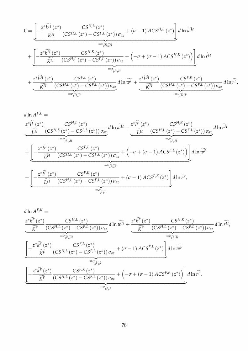
0 =

[−z∗kH (z∗)

KH

CSH,L (z∗)(CSH,L (z∗)− CSF,L (z∗)) σaz

+ (σ− 1) ACSH,L (z∗)

]︸ ︷︷ ︸

≡σkHwH

d ln wH

+

[−z∗kH (z∗)

KH

CSH,K (z∗)(CSH,L (z∗)− CSF,L (z∗)) σaz

+(−σ + (σ− 1) ACSH,K (z∗)

)]︸ ︷︷ ︸

≡σkH rH

d ln rH

+z∗kH (z∗)

KH

CSF,L (z∗)(CSH,L (z∗)− CSF,L (z∗)) σaz︸ ︷︷ ︸

≡σkHwF

d ln wF +z∗kH (z∗)

KH

CSF,K (z∗)(CSH,L (z∗)− CSF,L (z∗)) σaz︸ ︷︷ ︸

≡σkH rF

d ln rF,

d ln AF,L =

z∗ lF (z∗)

LH

CSH,L (z∗)(CSH,L (z∗)− CSF,L (z∗)) σaz︸ ︷︷ ︸

≡σlF wH

d ln wH +z∗ lF (z∗)

LH

CSH,K (z∗)(CSH,L (z∗)− CSF,L (z∗)) σaz︸ ︷︷ ︸

≡σlF rH

d ln rH

+

[−z∗ lF (z∗)

LH

CSF,L (z∗)(CSH,L (z∗)− CSF,L (z∗)) σaz

+(−σ + (σ− 1) ACSF,L (z∗)

)]︸ ︷︷ ︸

≡σlF wF

d ln wF

+

[−z∗ lF (z∗)

LH

CSF,K (z∗)(CSH,L (z∗)− CSF,L (z∗)) σaz

+ (σ− 1) ACSF,K (z∗)

]︸ ︷︷ ︸

≡σlF rF

d ln rF,

d ln AF,K =

z∗kF (z∗)

KF

CSH,L (z∗)(CSH,L (z∗)− CSF,L (z∗)) σaz︸ ︷︷ ︸

≡σkFwH

d ln wH +z∗kF (z∗)

KF

CSH,K (z∗)(CSH,L (z∗)− CSF,L (z∗)) σaz︸ ︷︷ ︸

≡σkF rH

d ln rH,

[−z∗kF (z∗)

KF

CSF,L (z∗)(CSH,L (z∗)− CSF,L (z∗)) σaz

+ (σ− 1) ACSF,L (z∗)

]︸ ︷︷ ︸

≡σkFwF

d ln wF

[−z∗kF (z∗)

KF

CSF,K (z∗)(CSH,L (z∗)− CSF,L (z∗)) σaz

+(−σ + (σ− 1) ACSF,K (z∗)

)]︸ ︷︷ ︸

≡σkF rF

d ln rF.

78

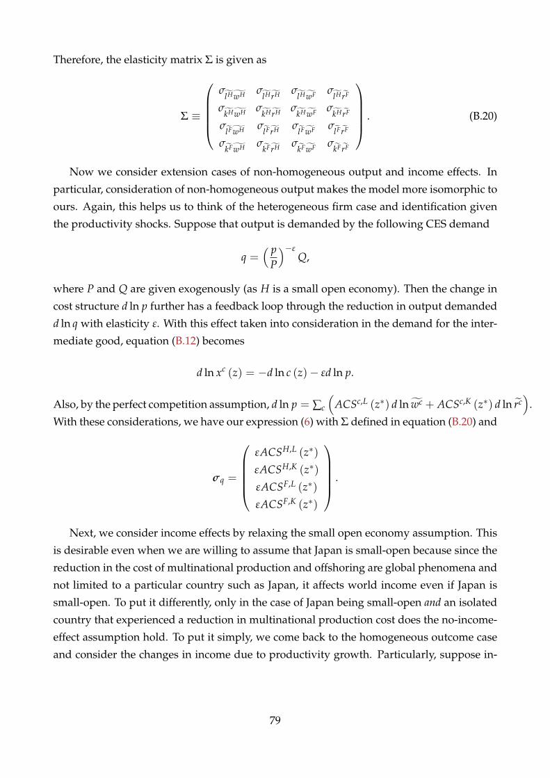
Therefore, the elasticity matrix Σ is given as

Σ ≡

σ

lHwH σlH rH σ

lHwF σlH rF

σkHwH σ

kH rH σkHwF σ

kH rF

σlFwH σ

lF rH σlFwF σlF rF

σkFwH σ

kF rH σkFwF σkF rF

. (B.20)

Now we consider extension cases of non-homogeneous output and income effects. In

particular, consideration of non-homogeneous output makes the model more isomorphic to

ours. Again, this helps us to think of the heterogeneous firm case and identification given

the productivity shocks. Suppose that output is demanded by the following CES demand

q =( p

P

)−εQ,

where P and Q are given exogenously (as H is a small open economy). Then the change in

cost structure d ln p further has a feedback loop through the reduction in output demanded

d ln q with elasticity ε. With this effect taken into consideration in the demand for the inter-

mediate good, equation (B.12) becomes

d ln xc (z) = −d ln c (z)− εd ln p.

Also, by the perfect competition assumption, d ln p = ∑c

(ACSc,L (z∗) d ln wc + ACSc,K (z∗) d ln rc

).

With these considerations, we have our expression (6) with Σ defined in equation (B.20) and

σq =

εACSH,L (z∗)

εACSH,K (z∗)

εACSF,L (z∗)

εACSF,K (z∗)

.

Next, we consider income effects by relaxing the small open economy assumption. This

is desirable even when we are willing to assume that Japan is small-open because since the

reduction in the cost of multinational production and offshoring are global phenomena and

not limited to a particular country such as Japan, it affects world income even if Japan is

small-open. To put it differently, only in the case of Japan being small-open and an isolated

country that experienced a reduction in multinational production cost does the no-income-

effect assumption hold. To put it simply, we come back to the homogeneous outcome case

and consider the changes in income due to productivity growth. Particularly, suppose in-

79

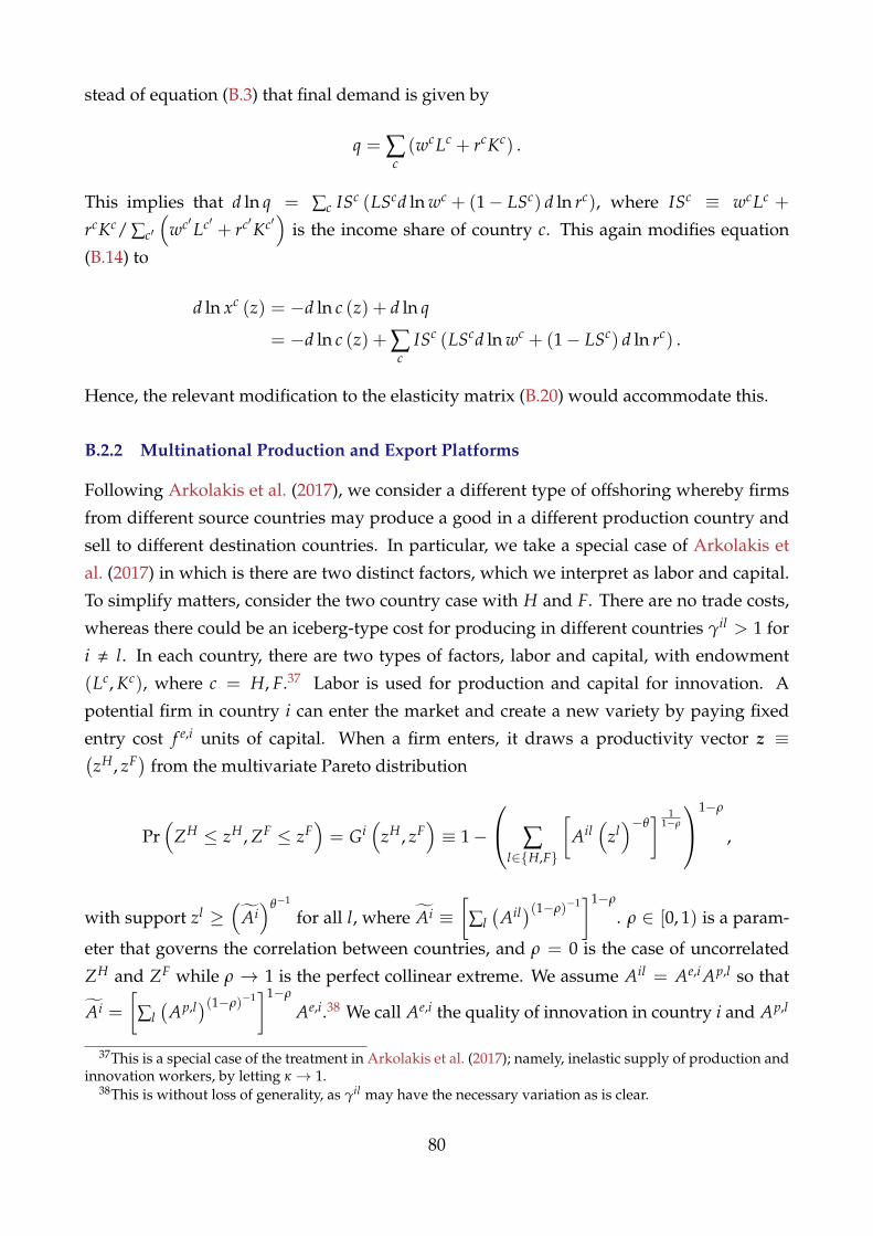
stead of equation (B.3) that final demand is given by

q = ∑c(wcLc + rcKc) .

This implies that d ln q = ∑c ISc (LScd ln wc + (1− LSc) d ln rc), where ISc ≡ wcLc +

rcKc/ ∑c′(

wc′Lc′ + rc′Kc′)

is the income share of country c. This again modifies equation

(B.14) to

d ln xc (z) = −d ln c (z) + d ln q

= −d ln c (z) + ∑c

ISc (LScd ln wc + (1− LSc) d ln rc) .

Hence, the relevant modification to the elasticity matrix (B.20) would accommodate this.

B.2.2 Multinational Production and Export Platforms

Following Arkolakis et al. (2017), we consider a different type of offshoring whereby firms

from different source countries may produce a good in a different production country and

sell to different destination countries. In particular, we take a special case of Arkolakis et

al. (2017) in which is there are two distinct factors, which we interpret as labor and capital.

To simplify matters, consider the two country case with H and F. There are no trade costs,

whereas there could be an iceberg-type cost for producing in different countries γil > 1 for

i , l. In each country, there are two types of factors, labor and capital, with endowment

(Lc, Kc), where c = H, F.37 Labor is used for production and capital for innovation. A

potential firm in country i can enter the market and create a new variety by paying fixed

entry cost f e,i units of capital. When a firm enters, it draws a productivity vector z ≡(zH, zF) from the multivariate Pareto distribution

Pr(

ZH ≤ zH, ZF ≤ zF)= Gi

(zH, zF

)≡ 1−

∑l∈{H,F}

[Ail(

zl)−θ

] 11−ρ

1−ρ

,

with support zl ≥(

Ai)θ−1

for all l, where Ai ≡[

∑l(

Ail)(1−ρ)−1]1−ρ

. ρ ∈ [0, 1) is a param-

eter that governs the correlation between countries, and ρ = 0 is the case of uncorrelated

ZH and ZF while ρ → 1 is the perfect collinear extreme. We assume Ail = Ae,i Ap,l so that

Ai =

[∑l(

Ap,l)(1−ρ)−1]1−ρ

Ae,i.38 We call Ae,i the quality of innovation in country i and Ap,l

37This is a special case of the treatment in Arkolakis et al. (2017); namely, inelastic supply of production andinnovation workers, by letting κ → 1.

38This is without loss of generality, as γil may have the necessary variation as is clear.

80

the productivity in production of country l.

ξ iln ≡ γilwlτln, (B.21)

Ψin ≡

∑l′

(Ail′

(ξ il′n

)−θ)(1−ρ)−1

1−ρ

(B.22)

ψiln ≡(

Til (ξ iln)−θ

Ψin

)(1−ρ)−1

(B.23)

Xiln = ψilnλE,inXn (B.24)

Miln =θ − σ + 1

σθ

Xiln

wnFn , (B.25)

λE,in ≡ ∑l Xiln

Xn . (B.26)

λT,ln ≡∑i

Xiln

Xn = ∑i

ψilnλE,in. (B.27)

We now characterize the equilibrium conditions that pin down(wH, rH, wF, rF) as follows.

The labor market equilibrium is given by the payment to workers equalling the sum of the

value of labor demand for production and marketing, as

1σ ∑

nλT,lnXn +

(1− η − 1

σ

)Xl = wl Ll (B.28)

for each l = H, F. The capital market equilibrium condition is such that the payment to

capital equals the value of capital demand for innovation, as

η ∑n

λE,inXn = riKi (B.29)

for each i = H, F. Finally, the budget balance condition is

wiLi + riKi + ∆i = Xi (B.30)

for each i = H, F, where ∆i is the transfer to country i from the ROW.

Consider a multinational production shock to the economy d ln γHF < 0. The log first-

order approximations to the system (B.28), (B.29), and (B.30) give

LDSl ∑n

PSln(

d ln λT,ln + d ln Xn)+(

1− LDSl)

d ln Xl = d ln wl, (B.31)

81

∑n

ISin(

d ln λE,in + d ln Xn)= d ln ri, (B.32)

LSid ln wi +(

1− LSi)

d ln ri = d ln Xi, (B.33)

where

LDSl ≡σ−1

σ ∑n λT,lnXn

σ−1σ ∑n λT,lnXn +

(1− η − σ−1

σ

)Xl

, PSln ≡ λT,lnXn

∑n′ λT,ln′Xn′ , ISin ≡ λE,inXn

∑n′ λE,in′Xn′

are the (value) labor demand share in production of each country, the production sales share

to country n, and innovation sales share to country n. Substituting equation (B.33) into

equations (B.31) and (B.32), we have

∑n

PSln(

d ln λT,ln + LSnd ln wn + (1− LSn) d ln rn)+ LSld ln wl +

(1− LSl

)d ln rl = d ln wl,

(B.34)

∑n

ISin(

d ln λE,in + LSnd ln wn + (1− LSn) d ln rn)= d ln ri. (B.35)

To study d ln λT,ln and d ln λE,in, first, by equation (B.27),

d ln λT,ln = ∑i

ψilnλE,in

∑i′ ψi′lnλE,i′n

(d ln ψiln + d ln λE,in

),

which, by equation (B.24), further simplifies to

d ln λT,ln = ∑i

Xiln

Xn

(d ln ψiln + d ln λE,in

). (B.36)

On the other hand, by equation (B.26), we have

d ln λE,in =(

1− λE,in) (

d ln Mi + d ln Ψin)− λE,in

(d ln Mi + d ln Ψin

). (B.37)

To further deduce, it remains to know d ln ψiln, d ln Mi, and d ln Ψin. By equations (B.21),

(B.22), (B.23), and (B.25), they are

d ln ψiln =1

1− ρ

(−θd ln ξ iln − d ln Ψin

),

=1

1− ρ

(−θd ln

(d ln wl + d ln γil

)− d ln Ψin

), (B.38)

82

d ln Ψin = ∑l′

ψil′n(−θd ln ξ il′n

),

= ∑l′

ψil′n(−θ(

d ln wl′ + d ln γil′))

, (B.39)

d ln Mi = ∑l′,n′

Mil′n′

Mi

(d ln Xil′n′ − d ln wn′

)(B.40)

= ∑l′,n′

Mil′n′

Mi

(d ln ψil′n′ + d ln λE,in′ + d ln Xn′ − d ln wn′

).

By substituting equations (B.36), (B.37), (B.38), (B.39), and (B.40), into equations (B.34) and

(B.35), we obtain an expression for

Σ

d ln wH

d ln rH

d ln wF

d ln rF

= b,

for a reduced demand elasticity matrix Σ and shock vector b.

B.3 Derivation of Equation (13)

The cost minimization problem under the upper nest implies

k =(

aK)σ−1

(rp

)−σ

q, and (B.41)

l =(

wp

)−σ

q, (B.42)

where pX ≡((

w/aL)1−λ+(

pM/aM)1−λ)1/(1−λ)

is the aggregate wage index and p ≡((r/aK)1−σ

+(

pX)1−σ)1/(1−σ)

is the marginal cost index. Similarly,

l = aL(

wpX

)−λ

l, and (B.43)

m = aM(

pM

pX

)−λ

l. (B.44)

83

By equating total demand to total supply, we have

K =(

aK)σ−1

(rp

)−σ

q⇔ r = p(

aK) σ−1

σ( q

K

) 1σ ,

X =

(pX

p

)−σ

q⇔ pX = p( q

X

) 1σ ,

L =(

aH)λ−1

(wpX

)−λ

X ⇔ w = pX(

aH) λ−1

λ

(XLH

) 1λ

,

M =(

aM)λ−1

(pM

pX

)−λ

X ⇔ pM = pX(

aM) λ−1

λ

(XM

) 1λ

.

By substituting these expressions,

LS ≡ wLwL + rK

=w(aL) λ−1

λ(X

L) 1

λ L

w (aL)λ−1

λ(X

L) 1

λ L + c (aK)σ−1

σ( q

K) 1

σ K

=c( q

L) 1

σ(aL) λ−1

λ(X

L) 1

λ L

c( q

X) 1

σ (aL)λ−1

λ(X

L) 1

λ L + c (aK)σ−1

σ( q

K) 1

σ K

=

(aLL)1−λ−1

Xλ−1−σ−1

(aLL)1−λ−1Xλ−1−σ−1 + (aKK)1−σ−1 .

B.4 Derivation of Equations (15) and (16)

We prove the effect of the shock with the following property: The shock decreases only the

foreign augmentation d ln aM < 0 but not capital and labor d ln aK = d ln aL = 0, and hits

only an infinitesimal set of firms so that factor prices are not affected. Note that perfect

competition implies the price is the marginal cost. Consider the following overall marginal

cost function

p =

(( raK

)1−σ+(

pX)1−σ

) 11−σ

=

( raK

)1−σ+

(( waL

)1−λ+

(pM

aM

)1−λ) 1−σ

1−λ

1

1−σ

.

Then the (first-order) elasticity of the cost with respect to log foreign factor-augmenting

productivity d ln AF is

d ln p = −CSM0 d ln aM,

84

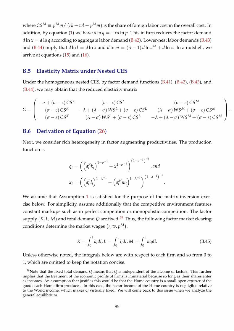
where CSM ≡ pMm/(rk + wl + pMm

)is the share of foreign labor cost in the overall cost. In

addition, by equation (1) we have d ln q = −εd ln p. This in turn reduces the factor demand

d ln x = d ln q according to aggregate labor demand (B.42). Lower-nest labor demands (B.43)

and (B.44) imply that d ln l = d ln x and d ln m = (λ− 1) d ln aM + d ln x. In a nutshell, we

arrive at equations (15) and (16).

B.5 Elasticity Matrix under Nested CES

Under the homogeneous nested CES, by factor demand functions (B.41), (B.42), (B.43), and

(B.44), we may obtain that the reduced elasticity matrix

Σ ≡

−σ + (σ− ε)CSK (σ− ε)CSL (σ− ε)CSM

(σ− ε)CSK −λ + (λ− σ)WSL + (σ− ε)CSL (λ− σ)WSM + (σ− ε)CSM

(σ− ε)CSK (λ− σ)WSL + (σ− ε)CSL −λ + (λ− σ)WSM + (σ− ε)CSM

.

B.6 Derivation of Equation (26)

Next, we consider rich heterogeneity in factor augmenting productivities. The production

function is

qi =

((aK

i ki

)1−σ−1

+ x1−σ−1

i

)(1−σ−1)−1

, and

xi =

((aL

i li)1−λ−1

+(

aMi mi

)1−λ−1)(1−λ−1)−1

.

We assume that Assumption 1 is satisfied for the purpose of the matrix inversion exer-

cise below. For simplicity, assume additionally that the competitive environment features

constant markups such as in perfect competition or monopolistic competition. The factor

supply (K, L, M) and total demand Q are fixed.39 Thus, the following factor market clearing

conditions determine the market wages(r, w, pM).

K =∫ 1

0kidi, L =

∫ 1

0lidi, M =

∫ 1

0midi. (B.45)

Unless otherwise noted, the integrals below are with respect to each firm and so from 0 to

1, which are omitted to keep the notation concise.

39Note that the fixed total demand Q means that Q is independent of the income of factors. This furtherimplies that the treatment of the economic profits of firms is immaterial because so long as their shares enteras incomes. An assumption that justifies this would be that the Home country is a small-open exporter of thegoods each Home firm produces. In this case, the factor income of the Home country is negligible relativeto the World income, which makes Q virtually fixed. We will come back to this issue when we analyze thegeneral equilibrium.

85

The cost-minimizing factor demands of firm i are

ki =(

aKi

)σ−1(

rpi

)−σ

qi, xi =

(pX

ipi

)−σ

qi, li =(

aLi

)λ−1(

wi

pXi

)−λ

xi, mi =(

aFi

)λ−1(

pMi

pXi

)−λ

xi,

where the marginal cost and aggregate labor-foreign input cost index are

pi =

( raK

i

)1−σ

+(

pXi

)1−σ

(1−σ)−1

, pXi =

( waL

i

)1−λ

+

(pM

aMi

)1−λ(1−λ)−1

. (B.46)

Substituting these into conditions (B.45), we have

K =∫ (

aKi

)σ−1(

rpi

)−σ ( pi

P

)−εQdi, (B.47)

L =∫ (

aLi

)λ−1(

wpX

i

)−λ(pX

ipi

)σ ( pi

P

)−εQdi, (B.48)

M =∫ (

aMi

)λ−1(

pM

pXi

)−λ(pX

ipi

)σ ( pi

P

)−εQdi. (B.49)

Since the system involves integrals of non-linear equations of unknowns(r, w, pM), the

closed-form solution is hardly tractable. We thus rely on our first order approximation

obtained in (6). Therefore, it suffices to know the log first-order approximation on w and r.

The log first-order approximations with respect to aM to the system (B.47), (B.48), and (B.49)

are

0 =∫ rki

rK(−σd ln r + (σ− ε) d ln pi) di,

0 =∫ wli

wL

(−λd ln w + (λ− σ) d ln pX

i + (σ− ε) d ln pi

)di,

0 =∫ pMmi

pM M

((λ− 1) d ln aM − λd ln pM + (λ− σ) d ln pX

i + (σ− ε) d ln pi

)di,

where, by equations (B.46) and cost-minimizing demand functions,

d ln pi =rki

piqid ln r +

pXi xi

piqid ln wi, and

d ln wi =wli

pXi xi

d ln wH +pMmi

pXi xi

d ln wF.

With slight abuse of notation, for Z = K, L, M and y = k, l, m, write CSZy as the employment

of factor y-weighted average of payment share to factor Z. For instance, with the home

86

labor (l) employment as the weight, the weighted average of the capital (K) payment share

is CSKl ≡

∫ wliwL

rkipiqi

di. Accordingly, for Z = L, M and y = l, m, write WSZy as the employment

of factor y-weighted average of wage payment share to factor Z.40 With these notations, we

can summarize the first-order approximation as the linear algebraic problem Az = b, where

A ≡

(σ− ε)CSK

k − σ (σ− ε)CSLk (σ− ε)CSM

k

(σ− ε)CSKl (λ− σ)WSL

l + (σ− ε)CSLl − λ (λ− σ)WSM

l + (σ− ε)CSMl

(σ− ε)CSKm (λ− σ)WSL

m + (σ− ε)CSLm (λ− σ)WSM

m + (σ− ε)CSMm − λ

,

(B.50)

z ≡

d ln r

d ln w

d ln pM

,

b ≡

(σ− ε)CSM

k

(λ− σ)WSMl + (σ− ε)CSM

l

(λ− σ)WSMl + (σ− ε)CSM

l − λ− (λ− 1)

d ln aM. (B.51)

Hence, if A is non-singular, z can be solved as z = A−1b and the log first-order approxi-

mation of labor share (6) can be solved accordingly. Indeed, equation (6) shows that only

x2 − x1 is our variable of interest.

To proceed, note that

z2 − z1 =3

∑j=1

(a−1

2j − a−11j

)bj,

where a−1ij is (i, j)-element of inverse matrix A−1. According to the formula of inverting

3× 3 matrices, we have

z2 − z1 ∝ {(a31 + a32) a23 − (a21 + a22) a33} b1

+ {(a11 + a12) a33 − (a31 + a32) a13} b2

+ {(a21 + a22) a13 − (a11 + a12) a23} b3

= (a11 + a12) (a33b2 − a23b3) + (a21 + a22) (a13b3 − a33b1)

(a31 + a32) (a23b1 − a13b2) .

Note that from equations (B.50) and (B.51), we have a13 = b1, a23 = b2, and a33 = b3 +

(λ− 1). Therefore, a33b2 − a23b3 = [b3 + (λ− 1)] b2 − b2b3 = (λ− 1) b2, a13b3 − a33b1 =

40Note the similarity of the definition to the one used in the homogeneous case in equation (14). WSXy

is the version that accommodates heterogeneity and contains the homogeneous case as a special case–withhomogeneous firms, WSX

y = WSX for any y, and WSF coincides with the one in equation (14).

87

b1b3 − [b3 + (λ− 1)] b1 = − (λ− 1) b1, and a23b1 − a13b2 = b2b1 − b1b2 = 0. Using these

facts, we further deduce that

z2 − z1 ∝ (a11 + a12) b2 + (a21 + a22) b1.

Substituting the elements in expressions (B.50) and (B.51), we finally have expression (26).

B.7 Derivation of Equations (27) and (28)

Here, we prove only equation (27), as (28) follows the same logic. First, recall that the

quantity-conditional factor demand cross derivatives ∂ki/∂ pMi |qi and ∂mi/∂ri|qi are equal

because (i) due to Shephard’s lemma, factor demands are the partial derivative of the

(quantity-conditional) cost function and (ii) the Hessian matrix is symmetric due to Young’s

theorem. Thus we have

σmr,i|qi ≡ri

mi

∂mi

∂ri|qi =

ri

mi

∂ki

∂ pMi

|qi =rki

pMmiσ

kpM,i|qi ,

where the last equality follows by definition σkpM,i|qi ≡

(pM

i /ki

) (∂ki/∂ pM

i |qi

)and the def-

initions of factor augmentation notations (tilde). By rearranging, we have

CSMi σmr,i|qi = CSK

i σkpM,i|qi . (B.52)

Finally, we have

σmr,i ≡ σmr,i|qi + σqp∂ ln pi

∂ ln ri

= σmr,i|qi + σqpCSKi ,

where the last equality again follows Shepard’s lemma. Similarly, we have σkpM,i

=

σkpM,i|qi + σqpCSM

i . Hence, we have

CSMi σmr,i = CSM

i σmr,i|qi + CSMi σqpCSK

i = CSKi σ

kpM,i|qi + CSK

i σqpCSMi = CSK

i σkpM,i

,

where the second equality holds by equation (B.52).

B.8 Properties of the Factor Demand Elasticity Matrix

Generalizing the results in Section B.7, we may establish the following result regarding off-

diagonal elements of the (quantity-controlled and -uncontrolled) elasticity matrix. We fur-

88

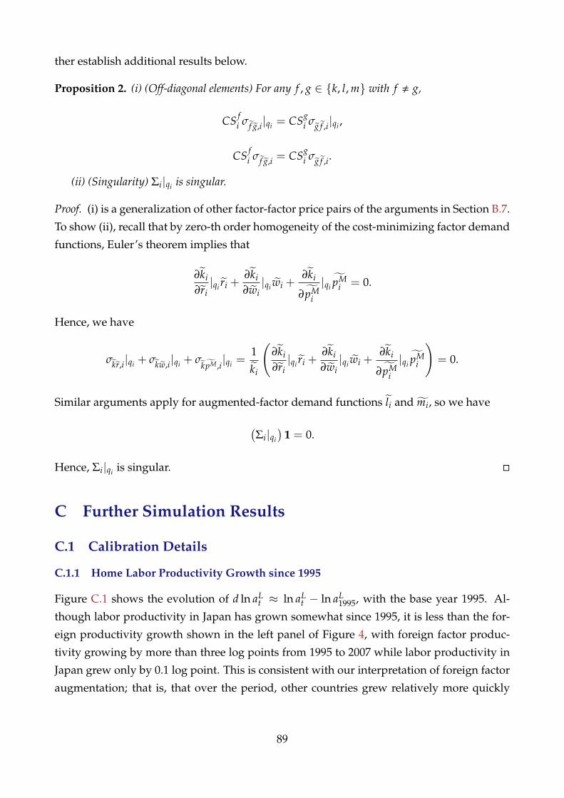
ther establish additional results below.

Proposition 2. (i) (Off-diagonal elements) For any f , g ∈ {k, l, m} with f , g,

CS fi σ f g,i|qi = CSg

i σg f ,i|qi ,

CS fi σ f g,i = CSg

i σg f ,i.

(ii) (Singularity) Σi|qi is singular.

Proof. (i) is a generalization of other factor-factor price pairs of the arguments in Section B.7.

To show (ii), recall that by zero-th order homogeneity of the cost-minimizing factor demand

functions, Euler’s theorem implies that

∂ki

∂ri|qi ri +

∂ki

∂wi|qi wi +

∂ki

∂ pMi

|qi pMi = 0.

Hence, we have

σkr,i|qi + σkw,i|qi + σkpM,i|qi =

1

ki

(∂ki

∂ri|qi ri +

∂ki

∂wi|qi wi +

∂ki

∂ pMi

|qi pMi

)= 0.

Similar arguments apply for augmented-factor demand functions li and mi, so we have

(Σi|qi

)1 = 0.

Hence, Σi|qi is singular. �

C Further Simulation Results

C.1 Calibration Details

C.1.1 Home Labor Productivity Growth since 1995

Figure C.1 shows the evolution of d ln aLt ≈ ln aL

t − ln aL1995, with the base year 1995. Al-

though labor productivity in Japan has grown somewhat since 1995, it is less than the for-

eign productivity growth shown in the left panel of Figure 4, with foreign factor produc-

tivity growing by more than three log points from 1995 to 2007 while labor productivity in

Japan grew only by 0.1 log point. This is consistent with our interpretation of foreign factor

augmentation; that is, that over the period, other countries grew relatively more quickly

89

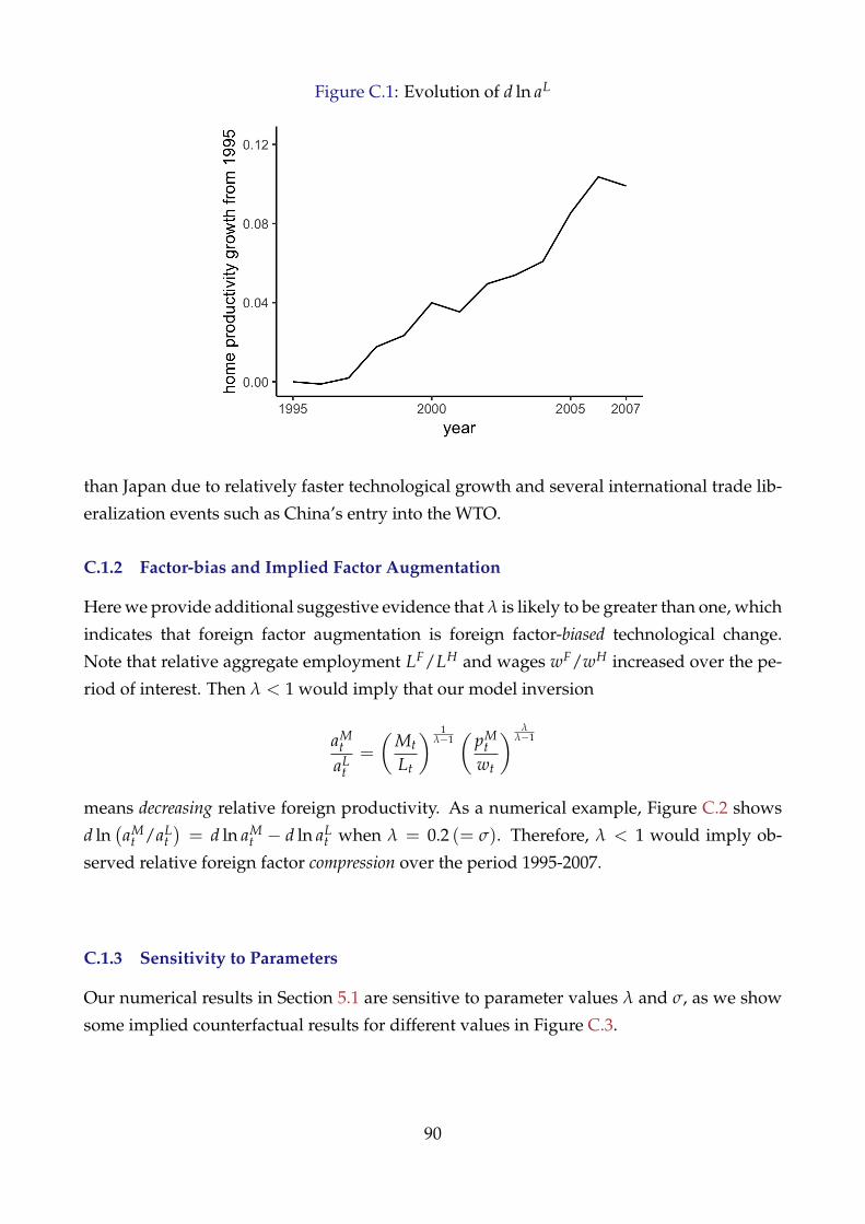
Figure C.1: Evolution of d ln aL

than Japan due to relatively faster technological growth and several international trade lib-

eralization events such as China’s entry into the WTO.

C.1.2 Factor-bias and Implied Factor Augmentation

Here we provide additional suggestive evidence that λ is likely to be greater than one, which

indicates that foreign factor augmentation is foreign factor-biased technological change.

Note that relative aggregate employment LF/LH and wages wF/wH increased over the pe-

riod of interest. Then λ < 1 would imply that our model inversion

aMt

aLt=

(Mt

Lt

) 1λ−1(

pMt

wt

) λλ−1

means decreasing relative foreign productivity. As a numerical example, Figure C.2 shows

d ln(aM

t /aLt)= d ln aM

t − d ln aLt when λ = 0.2 (= σ). Therefore, λ < 1 would imply ob-

served relative foreign factor compression over the period 1995-2007.

C.1.3 Sensitivity to Parameters

Our numerical results in Section 5.1 are sensitive to parameter values λ and σ, as we show

some implied counterfactual results for different values in Figure C.3.

90

Figure C.2: Implied aM Trend When λ = σ = 0.2

C.2 Implications of a More Recent Trend, 1995-2015

The 2008SNA from the Japan Cabinet Office provides System of National Accounts (SNA)

data for 1994-2015. The 2008SNA introduced many modifications to the previous SNAs,

among them the capitalization of Research and Development (R&D) expenditures which,

for our purposes, bumps up value added and drives down labor share.

Another qualification regarding the use of the more recent trend is the Great Recession

that began in 2008 which empirically shows a halt in the reduction in labor share in the

mid 2000s that is consistent with a widely found fact that labor share is countercyclical

(Schneider, 2011). Since our focus is the structural change in foreign factor augmentation,

we do not emphasize this period, but as described below, our mechanism of relative factor

substitution of labor might help to explain this countercyclicality.

Figure C.4 shows the actual and counterfactual labor share trends derived by the same

exercise as in Figure 5b. As mentioned above, while labor share has generally been de-

creasing, there was a halt in the decline in the mid 2000s to early 2010s. Remarkably, the

counterfactual trend shows a similar pattern of an overall decline that paused during the

Great Recession. To understand this, recall that an important factor driving the changes in

the counterfactual trend is the observed foreign factor augmentation (e.g., equation (25)),

which is backed out by relative foreign employment and wages. To the extent that dur-

ing the Great Recession globalization halted and MNE multinational activities stalled, the

measured foreign factor augmentation process slowed down and even reversed, which is

consistent with the slow-down and increase in counterfactual labor share seen in Figure

C.4. Although we do not centralize this hypothesis in the current paper, a more thorough

91

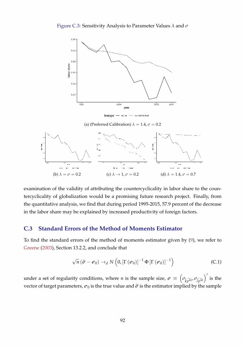
Figure C.3: Sensitivity Analysis to Parameter Values λ and σ

(a) (Preferred Calibration) λ = 1.4, σ = 0.2

(b) λ = σ = 0.2 (c) λ→ 1, σ = 0.2 (d) λ = 1.4, σ = 0.7

examination of the validity of attributing the countercyclicality in labor share to the coun-

tercyclicality of globalization would be a promising future research project. Finally, from

the quantitative analysis, we find that during period 1995-2015, 57.9 percent of the decrease

in the labor share may be explained by increased productivity of foreign factors.

C.3 Standard Errors of the Method of Moments Estimator

To find the standard errors of the method of moments estimator given by (9), we refer to

Greene (2003), Section 13.2.2, and conclude that

√n (σ − σ0)→d N

(0, [Γ (σ0)]

−1 Φ [Γ (σ0)]−1)

(C.1)

under a set of regularity conditions, where n is the sample size, σ ≡(

σkpM , σ

l pM

)′is the

vector of target parameters, σ0 is the true value and σ is the estimator implied by the sample

92

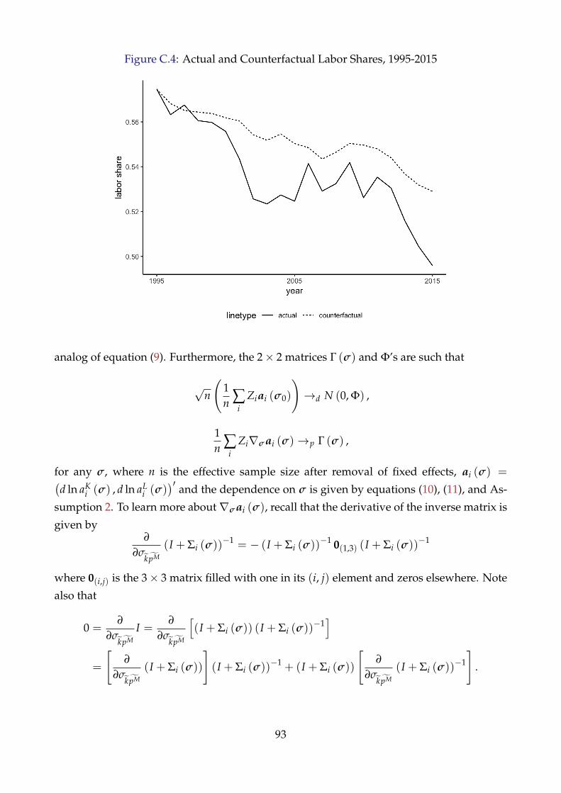
Figure C.4: Actual and Counterfactual Labor Shares, 1995-2015

analog of equation (9). Furthermore, the 2× 2 matrices Γ (σ) and Φ’s are such that

√n

(1n ∑

iZiai (σ0)

)→d N (0, Φ) ,

1n ∑

iZi∇σai (σ)→p Γ (σ) ,

for any σ, where n is the effective sample size after removal of fixed effects, ai (σ) =(d ln aK

i (σ) , d ln aLi (σ)

)′ and the dependence on σ is given by equations (10), (11), and As-

sumption 2. To learn more about∇σai (σ), recall that the derivative of the inverse matrix is

given by∂

∂σkpM

(I + Σi (σ))−1 = − (I + Σi (σ))

−1 0(1,3) (I + Σi (σ))−1

where 0(i,j) is the 3× 3 matrix filled with one in its (i, j) element and zeros elsewhere. Note

also that

0 =∂

∂σkpM

I =∂

∂σkpM

[(I + Σi (σ)) (I + Σi (σ))

−1]

=

[∂

∂σkpM

(I + Σi (σ))

](I + Σi (σ))

−1 + (I + Σi (σ))

[∂

∂σkpM

(I + Σi (σ))−1

].

93

Using these, we may solve

∇σai (σ) =

(∂

∂σkpM

ai (σ) ,∂

∂σl pM

ai (σ)

)

and∂

∂σkpM

ai (σ) = I−(3,·) (I + Σi (σ))−1 0(1,3) (I + Σi (σ))

−1 pi,

∂

∂σl pM

ai (σ) = I−(3,·) (I + Σi (σ))−1 0(2,3) (I + Σi (σ))

−1 pi,

where

I−(3,·) ≡(

1 0 0

0 1 0

), pi =

d ln (rki)

d ln (wli)

d ln(

pMmi) .

To estimate Φ and Γ (σ), we use their sample analogs Φ and Γ (σ)

Φj1,j2 =1

n− 1 ∑i

Z2i d ln aj1

i (σ) d ln aj2i (σ) ,

Γ (σ) =1n ∑

iZi∇σai (σ) ,

where j1, j2 ∈ {K, L}. We evaluate Γ at the estimated parameter value σ = σ, and then

estimate the finite approximation of the asymmetric distribution of the estimator (C.1) by

1n

[Γ (σ)

]−1Φ[Γ (σ)

]−1.

References for Appendix

Acemoglu, Daron and Pascual Restrepo, “Automation and New Tasks: How Technology

Displaces and Reinstates Labor,” Technical Report, National Bureau of Economic Re-

search 2019.

Arkolakis, Costas, Natalia Ramondo, Andres Rodrıguez-Clare, and Stephen Yeaple, “In-

novation and Production in the Global Economy,” 2017.

Bartik, Timothy J, “Who benefits from state and local economic development policies?,”

1991.

94

Benguria, Felipe and Alan M Taylor, “After the Panic: Are Financial Crises Demand or

Supply Shocks? Evidence from International Trade,” Working Paper 25790, National Bu-

reau of Economic Research April 2019.

Bridgman, Benjamin, “Is Labor’s Loss Capital’s Gain? Gross Versus Net Labor Shares,”

Macroeconomic Dynamics, 2018, 22 (08), 2070–2087.

Caballero, Ricardo J, Emmanuel Farhi, and Pierre-Olivier Gourinchas, “Rents, technical

change, and risk premia accounting for secular trends in interest rates, returns on capital,

earning yields, and factor shares,” American Economic Review, 2017, 107 (5), 614–20.

Carvalho, Vasco M, Makoto Nirei, Yukiko U Saito, and Alireza Tahbaz-Salehi, “Supply

chain disruptions: Evidence from the great east japan earthquake,” 2016.

Debreu, Gerard, “Excess demand functions,” Journal of mathematical economics, 1974, 1 (1),

15–21.

Desai, Mihir A, C Fritz Foley, and James R Hines, “Domestic effects of the foreign activities

of US multinationals,” American Economic Journal: Economic Policy, 2009, 1 (1), 181–203.

Feenstra, Robert C and Gordon H Hanson, “Foreign direct investment and relative wages:

Evidence from Mexico’s maquiladoras,” Journal of international economics, 1997, 42 (3), 371–

393.

Fort, Teresa C, Justin R Pierce, and Peter K Schott, “New perspectives on the decline of us

manufacturing employment,” Journal of Economic Perspectives, 2018, 32 (2), 47–72.

Goldsmith-Pinkham, Paul, Isaac Sorkin, and Henry Swift, “Bartik instruments: What,

when, why, and how,” Technical Report, National Bureau of Economic Research 2018.

Greene, William H, Econometric analysis, Pearson Education India, 2003.

Greenwald, Daniel L, Martin Lettau, and Sydney C Ludvigson, “How the Wealth Was

Won: Factors Shares as Market Fundamentals,” Working Paper 25769, National Bureau of

Economic Research April 2019.

Harrison, Ann and Margaret McMillan, “Offshoring jobs? Multinationals and US manu-

facturing employment,” Review of Economics and Statistics, 2011, 93 (3), 857–875.

Hirakata, Naohisa and Yasutaka Koike, “The Labor Share, Capital-Labor Substitution, and

Factor Augmenting Technologies,” Technical Report, Bank of Japan 2018.

Hubmer, Joachim, “The Race Between Preferences and Technology,” Technical Report,

mimeo, Yale University 2018.

95

Hummels, David, Rasmus Jørgensen, Jakob Munch, and Chong Xiang, “The wage effects

of offshoring: Evidence from Danish matched worker-firm data,” American Economic Re-

view, 2014, 104 (6), 1597–1629.

Karabarbounis, Loukas and Brent Neiman, “The global decline of the labor share,” The

Quarterly journal of economics, 2013, 129 (1), 61–103.

Kirimura, T, T Nakaya, and K Yano, “Building a spatio-temporal GIS database about

boundaries of municipalities: municipality Map Maker for Web,” Theory Appl GIS, 2011,

19, 83–92.

Loecker, Jan De and Jan Eeckhout, “The rise of market power and the macroeconomic

implications,” Technical Report, National Bureau of Economic Research 2017.

and , “Global market power,” Technical Report, National Bureau of Economic Research

2018.

Mantel, Rolf R, “On the characterization of aggregate excess demand,” Journal of economic

theory, 1974, 7 (3), 348–353.

Mas-Colell, Andreu, Michael Dennis Whinston, Jerry R Green et al., Microeconomic theory,

Vol. 1, Oxford university press New York, 1995.

Oberfield, Ezra and Devesh Raval, “Micro data and macro technology,” Technical Report,

National Bureau of Economic Research 2014.

Olley, G Steven and Ariel Pakes, “The Dynamics of Productivity in the Telecommunica-

tions Equipment Industry,” Econometrica, 1996, 64 (6), 1263–1297.

Pierce, Justin R and Peter K Schott, “The surprisingly swift decline of US manufacturing

employment,” American Economic Review, 2016, 106 (7), 1632–62.

Raval, Devesh R, “The micro elasticity of substitution and non-neutral technology,” The

RAND Journal of Economics, 2019, 50 (1), 147–167.

Rognlie, Matthew, “Comment on” Accounting for Factorless Income”,” in “NBER Macroe-

conomics Annual 2018, volume 33,” University of Chicago Press, 2018.

Schneider, Dorothee, “The labor share: A review of theory and evidence,” Technical Report,

SFB 649 discussion paper 2011.

Sonnenschein, Hugo, “Market excess demand functions,” Econometrica: Journal of the Econo-

metric Society, 1972, pp. 549–563.

96

Table A.11: Industry-level Regression

(a) 2SLS

(1) (2) (3) (4) (5) (6)VARIABLES 2SLS 2SLS 2SLS 2SLS 2SLS 2SLS

Log Subsidiary Employment 0.120** -0.00447 0.168*** 0.0774 -0.184 0.507*(0.0501) (0.610) (0.0486) (0.0694) (0.162) (0.292)

Observations 3,704 773 540 563 521 915Firm FE YES YES YES YES YES YESYear FE YES YES YES YES YES YESIndustry manuf chem metal machine elec auto

Robust standard errors in parentheses*** p<0.01, ** p<0.05, * p<0.1

(1) (2) (3) (4) (5) (6)VARIABLES 1st 1st 1st 1st 1st 1st

Thai Flood Shock -0.730*** -0.152 -1.655*** -2.223** -0.655*** -0.303**(0.169) (0.173) (0.358) (1.101) (0.161) (0.132)

Observations 3,704 773 540 563 521 915Firm FE YES YES YES YES YES YESYear FE YES YES YES YES YES YESIndustry manuf chem metal machine elec auto

Robust standard errors in parentheses*** p<0.01, ** p<0.05, * p<0.1

(b) First Stage

(1) (2) (3) (4) (5) (6)VARIABLES reduced reduced reduced reduced reduced reduced

Thai Flood Shock -0.0874** 0.000677 -0.277*** -0.172 0.120 -0.154**(0.0428) (0.0923) (0.0594) (0.225) (0.105) (0.0700)

Observations 3,704 773 540 563 521 915Firm FE YES YES YES YES YES YESYear FE YES YES YES YES YES YESIndustry manuf chem metal machine elec auto

Robust standard errors in parentheses*** p<0.01, ** p<0.05, * p<0.1

(c) Reduced Form

97